introduction to algebraic topologymsc.tsinghua.edu.cn/sli/algebraic-topology.pdf · this is course...
TRANSCRIPT
INTRODUCTION TO ALGEBRAIC TOPOLOGY
SI LI
ABSTRACT. To be continued. This is course note for Algebraic Topology in Spring 2018 at Tsinghua university.
Coure References:
(1) Hatcher: Algebraic Topology(2) Bott and Tu: Differential forms in algebraic topology.(3) May: A Concise Course in Algebraic Topology(4) Spanier: Algebraic Topology.
CONTENTS
1. Category and Functor 2
2. Fundamental Groupoid 5
3. Covering and fibration 7
4. π1(S1) and applications 9
5. Classification of covering 11
6. Seifert-van Kampen Theorem 14
7. Path space and homotopy fiber 15
8. Group object and homotopy group 19
9. Exact Puppe sequence 21
10. Cofibration 24
11. CW complex 27
12. Whitehead Theorem 29
13. Cellular and CW approximations 32
14. Eilenberg-MacLane Space 34
15. Singular Homology 36
16. Exact homology sequence 39
17. Excision 41
18. Homology of spheres 44
19. Cellular homology 46
20. Cohomology and Universal Coefficient Theorem 491
2 SI LI
21. Eilenberg-Zilber Theorem and Kunneth formula 53
22. Cup and Cap product 56
23. Poincare duality 60
24. Intersection and Lefschetz Fixed Point Theorem 63
1. CATEGORY AND FUNCTOR
Category.
Definition 1.1. A category C consists of
(1) a class of objects: Obj(C)(2) morphisms: a set HomC(A, B), ∀A, B ∈ Obj(C). An element f ∈ Hom(A, B) will be denoted by
Af→ B or f : A→ B.
(3) composition:
Hom(A, B)×Hom(B, C)→ Hom(A, C), ∀A, B, C ∈ Obj(C)
f × g→ g f
satisfying the following axioms
(1) associativity: h (g f ) = (h g) f for any Af→ B
g→ C h→ D.(2) identity: ∀A ∈ Obj(C), ∃1A ∈ Hom(A, A) called the identity element, such that
f 1A = f = 1B f , ∀Af→ B.
A category is called small if its objects form a set.
Definition 1.2. A morphism f : A→ B is called an equivalence/invertible if ∃g : B→ A such that
f g = 1B, g f = 1A.
Two objects A, B are called equivalent if there exists an equivalence f : A→ B.
Definition 1.3. A category where all morphisms are equivalences is called a groupoid.
Definition 1.4. A subcategory C ′ ⊂ C is a category such that
• Obj(C ′) ⊂ Obj(C)• HomC ′(A, B) ⊂ HomC(A, B), ∀A, B ∈ Obj(C ′)• composition coincides.
C ′ is called a full subcategory of C if HomC ′(A, B) = HomC(A, B), ∀A, B ∈ Obj(C ′).
Definition 1.5. Let ∼ be an equivalence relation defined on each Hom(A, B), A, B ∈ Obj(C) satisfying
f1 ∼ f2, g1 ∼ g2 =⇒ g1 f1 ∼ g2 f2.
Then we define the quotient category C ′ = C/ ∼ by
• Obj(C ′) = Obj(C ′)
INTRODUCTION TO ALGEBRAIC TOPOLOGY 3
• HomC ′(A, B) = HomC(A, B)/ ∼, ∀A, B ∈ Obj(C ′)
Example 1.6. We will frequently use the following categories.
• Set: the category of set.• Vect: the category of vector spaces.• Group: the category of groups.• Ab: the category of abelian groups.• Ring: the category of rings.
Vect ⊂ Set is a subcategory, and Ab ⊂ Group is a full subcategory.
The main object of our interest is the category of topological spaces Top
• objects of Top are topological spaces.• morphism f : X → Y is a continuous map.
Definition 1.7. Given X, Y ∈ Top, f0, f1 : X → Y are said to to homotopic, denoted by f0 ' f1, if
∃F : X× I → Y, such that F|X×0 = f0, F|X×1 = f1. I = [0, 1].
Homotopy defines an equivalence relation on Top. We denote its quotient category by
hTop = Top / ' .
We also denoteHomhTop(X, Y) = [X, Y].
Definition 1.8. Two topological spaces X, Y are said to have the same homotopy type (or homotopy equiv-alent) if they are equivalent in hTop.
There is also a relative version as follows.
Definition 1.9. Let A ⊂ X ∈ Top, f0, f1 : X → Y such that f0|A = f1|A : A → Y. We say f0 is homotopic tof1 relative to A, denoted by
f0 ' f1 rel A
if there exists F : X× I → Y such that
F|X×0 = f0, F|X×1 = f1, F|A×t = f0|A, ∀t ∈ I.
Functor.
Definition 1.10. Let C,D be two categories. A covariant functor (or contravariant functor) F : C → Dconsists of
• F : Obj(C)→ Obj(D), A→ F(A)
• HomC(A, B)→ HomD(F(A), F(B)), ∀A, B ∈ Obj(C). We denote by
Af→ B =⇒ F(A)
F( f )→ F(B)
( or HomC(A, B)→ HomD(F(B), F(A)), ∀A, B ∈ Obj(C), denoted by Af→ B =⇒ F(B)
F( f )→ F(A) )
satisfying
• F(g f ) = F(g) F( f ) (or F(g f ) = F( f ) F(g)) for any Af→ B
g→ C
4 SI LI
• F(1A) = 1F(A), ∀A ∈ Obj(C).
F is called faithful (or full) if HomC(A, B)→ HomD(F(A), F(B)) is injective (or surjective) ∀A, B ∈ Obj(C).
Example 1.11. ∀X ∈ Obj(C),
Hom(X,−) : C → Set, A→ Hom(X, A)
defines a covariant functor. Similarly Hom(−, X) defines a contravariant functor. A functor F : C → Set ofsuch type is called representable.
Example 1.12. Let G be an abelian group. Given X ∈ Top, we will study its n-th cohomology Hn(X; G). Itdefines a functor
Hn(−; G) : hTop→ Set, X → Hn(X; G)
We will see that this functor is representable by the Eilenberg-Maclane space if we work with the subcate-gory of CW-complexes.
Example 1.13. We define a contravariant functor
Fun : Top→ Ring, X → Fun(X) = Hom(X, R)
F(X) are continuous real functions on X. A classical theorem of Gelfand-Kolmogoroff says that two compactHausdorff spaces X, Y are homeomorphic if and only if Fun(X), Fun(Y) are ring isomorphic.
Proposition 1.14. Let F : C → D be a functor. f : A→ B is an equivalence. Then F( f ) : F(A)→ F(B) is also anequivalence.
Natural transformation.
Definition 1.15. Let C,D be two categories. F, G : C → D be two functors. A natural transformationτ : F → G consists of morphisms
τ = τA : F(A)→ G(A)|∀A ∈ Obj(C)
such that the following diagram commutes for any A, B ∈ Obj(C)
F(A)
τA
F( f )// F(B)
τB
G(A)G( f )
// G(B)
τ is called natural equivalence if τA is an equivalence for any A ∈ Obj(C). We write F ' G.
Definition 1.16. Two categories C,D are called isomorphic if ∃F : C → D, G : D → C such that F G =
1D , G F = 1C . They are called equivalent if ∃F : C → D, G : D → C such that F G ' 1D , G F ' 1C
Proposition 1.17. Let F : C → D be an equivalence of categories. Then F is fully faithful.
Definition 1.18. Let C be a small category, and D be a category. We define the functor category Fun(C,D)
• objects: covariant functors from C to D• morphism: natural transformations between two functors (which is indeed a set since C is small).
INTRODUCTION TO ALGEBRAIC TOPOLOGY 5
2. FUNDAMENTAL GROUPOID
Path connected component.
Definition 2.1. Let X ∈ Top. A map γ : I → X is called a path from γ(0) to γ(1). We denote γ−1 be thepath from γ(1) to γ(0) defined by γ−1(t) = γ(1− t). We denote ix0 : I → X be the constant map to x0 ∈ X.
Let us introduce an equivalence relation on X by
x0 ∼ x1 ⇐⇒ ∃ a path from x0 to x1.
We denote the quotient spaceπ0(X) = X/ ∼
which is the set of path connected components of X.
Proposition 2.2. π0 : hTop→ Set defines a covariant functor.
As a consequence, π0(X) ∼= π0(Y) if X, Y are homotopy equivalent.
Path category/fundamental groupoid.
Definition 2.3. Let γ : I → X be a path. We define the path class of γ
[γ] = γ : I → X|γ ' γ rel ∂I = 0, 1
Definition 2.4. Let γ1, γ2 : I → X such that γ1(1) = γ2(0). We define
γ2 ? γ1 : I → X
by
γ2 ? γ1(t) =
γ1(2t) 0 ≤ t ≤ 1/2
γ2(2t− 1) 1/2 ≤ t ≤ 1.
? is not associative for strict paths. However, ? defines an associative composition on path classes.
Theorem 2.5. Let X ∈ Top. We define a category Π1(X) as follows:
• Obj(Π1(X)) = X.• HomΠ1(X)(x0, x1)=path classes from x0 to x1.• 1x0 = ix0 .
Then Π1(X) defines a category which is in fact a groupoid. The inverse of [γ] is given by [γ−1]. Π1(X) is called thefundamental groupoid of X.
Let C be a groupoid. Let A ∈ Obj(C), then
AutC(A) := HomC(A, A)
forms a group. For any f : A→ B, it induces a group isomorphism
Ad f : AutC(A)→ AutC(B)
g→ f g f−1.
This naturally defines a functor
C → Group
6 SI LI
A→ AutC(A)
f → Ad f
Specialize this to topological spaces, we find a functor
Π1(X)→ Group .
Definition 2.6. Let x0 ∈ X, the group
π1(X, x0) := AutΠ1(X)(x0)
is called the fundamental group of the pointed space (X, x0).
Theorem 2.7. Let X be path connected. Then for x0, x1 ∈ X, the have group isomorphism
π1(X, x0) ∼= π1(X, x1).
Let f : X → Y be a continuous map. It defines a functor
Π1( f ) : Π1(X)→ Π1(Y)
x → f (x)
[γ]→ [ f γ].
Then Π1 defines a functor
Π1 : Top→ Groupoid , X → Π1(X)
from the category Top to the category Groupoid of groupoids. Here morphisms in Groupoid are given bynatural transformations.
Proposition 2.8. Let f , g : X → Y be maps which are homotopic by F : X× I → Y. Let us define path classes
τx0 = [F|x0×I ] ∈ HomΠ1(Y)( f (x0), g(x0)).
Then τ defines a natural transformation
τ : Π1( f ) =⇒ Π1(g).
This proposition can be pictured by the following diagram
Xf&&
g88 F Y =⇒ Π1(X)
Π1( f ) ++
Π1(g)33
τ Π1(Y)
The following theorem is a formal consequence of the above proposition
Theorem 2.9. Let f : X → Y be a homotopy equivalence. Then
Π1( f ) : Π1(X)→ Π1(Y)
is an equivalence of categories. In particular, it induces group isomorphisms
π1(X, x0) ∼= π1(Y, f (x0)),
INTRODUCTION TO ALGEBRAIC TOPOLOGY 7
3. COVERING AND FIBRATION
Covering.
Definition 3.1. Let p : E→ B be continuous. A trivialization of p over an open U ⊂ B is a homeomorphismϕ : p−1(U)→ U × F over U, i.e. , the following diagram commutes
p−1(U)ϕ
//
""
U × F
||U
p is called locally trivial if there exists an open cover U of B such that p has a trivialization over each openU ∈ U . Such p is also called a fiber bundle and F is called the fiber.
Definition 3.2. A covering is a locally trivial map p : E→ B with discrete fiber F.
Example 3.3. ex : R1 → S1, t→ e2πit is a covering.
Definition 3.4. Let p : E→ B, f : X → B. A lifting of f along p is a map F : X → E such that p F = f
E
p
X
F??
f// B
Lemma 3.5. Let p : E→ B be a covering. Let
D = (x, x) ∈ E× E|x ∈ E
Z = (x, y) ∈ E× E|p(x) = p(y).
Then D ⊂ Z is open and closed.
Theorem 3.6 (Uniqueness of lifting). Let p : E → B be a covering. Let F0, F1 : X → E be two liftings of f .Suppose X is connected and F0, F1 agree somewhere. Then F0 = F1.
Proof. Consider the map F = (F0, F1) : X → Z. F(X) ∩ D 6= ∅. The above lemma implies F(X) ⊂ D.
fibration.
Definition 3.7. A map p : E → B is said to have the homotopy lifting property (HLP) with respect to X iffor any maps f : X → E and F : X× I → B such that p f = F|X×0, there exists a lifting F of F along p suchthat F|X×0 = f , i.e., the following diagram commutes
X× 0f//
_
E
p
X× IF//
∃F<<
B
Definition 3.8. A map p : E→ B is called a fibration (or Hurewicz fibration) if p has HLP for any space.
Theorem 3.9. A covering is a fibration .
8 SI LI
Corollary 3.10. Let p : E→ B be a fibration. Then for any path γ : I → B and e ∈ E such that p(e) = γ(0), thereexists a unique path γ : I → E that lifts γ and γ(0) = e.
Proof. Apply HLP to X=pt.
0e //
_
E
p
Iγ//
γ@@
B
Corollary 3.11. Let p : E→ B be a covering. Then Π1(E)→ Π1(B) is a faithful functor. In particular, the inducedmap π1(E, e)→ π1(B, p(e)) is injective.
Transport functor.
Let p : E→ B be a covering. Let γ : I → B be a path in B from b1 to b2. It defines a map
Tγ : p−1(b1)→ p−1(b2)
e1 → γ(1)
where γ is a lift of γ with initial condition γ(0) = e1.
Assume [γ1] = [γ2] in B. HLP implies that Tγ1 = Tγ2 . We find a well-defined map
T : HomΠ1(B)(b1, b2)→ HomSet(p−1(b1), p−1(b2))
[γ]→ T[γ]
Proposition 3.12. The following data
T : Π1(B)→ Set
b→ p−1(b)
[γ]→ T[γ].
defines a functor, called the transport functor. In particular, we have a well-defined map
π1(B, b)→ Aut(p−1(b)).
Proposition 3.13. Let p : E → B be a covering, E path connected. Let e ∈ E, b = p(e) ∈ B. Then the action ofπ1(B, b) on p−1(b) is transitive, whose stabilizer at e is π1(E, e). In other words,
p−1(b) ∼= π1(B, b)/π1(E, e)
as a coset space.
Lifting Criterion.
Theorem 3.14 (Lifting Criterion). Let p : E → B be a covering. f : X → B for X path connected and locally pathconnected. Let e ∈ E, x0 ∈ X such that f (x0) = p(e). Then there exists a lift F of f with F(x0) = e if and only if
f∗(π1(X, x0)) ⊂ p∗(π1(E, e)).
INTRODUCTION TO ALGEBRAIC TOPOLOGY 9
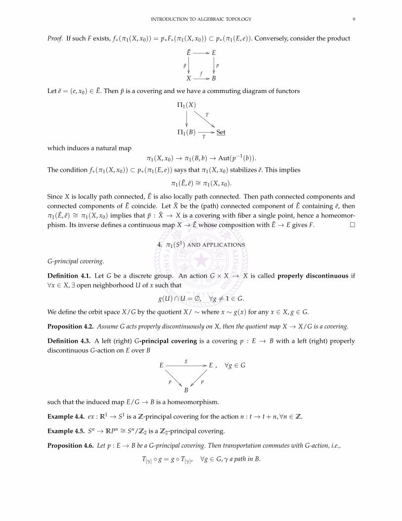
Proof. If such F exists, f∗(π1(X, x0)) = p∗F∗(π1(X, x0)) ⊂ p∗(π1(E, e)). Conversely, consider the product
E
p
// E
p
Xf// B
Let e = (e, x0) ∈ E. Then p is a covering and we have a commuting diagram of functors
Π1(X)
T
""Π1(B)
T// Set
which induces a natural map
π1(X, x0)→ π1(B, b)→ Aut(p−1(b)).
The condition f∗(π1(X, x0)) ⊂ p∗(π1(E, e)) says that π1(X, x0) stabilizes e. This implies
π1(E, e) ∼= π1(X, x0).
Since X is locally path connected, E is also locally path connected. Then path connected components andconnected components of E coincide. Let X be the (path) connected component of E containing e, thenπ1(E, e) ∼= π1(X, x0) implies that p : X → X is a covering with fiber a single point, hence a homeomor-phism. Its inverse defines a continuous map X → E whose composition with E→ E gives F.
4. π1(S1) AND APPLICATIONS
G-principal covering.
Definition 4.1. Let G be a discrete group. An action G × X → X is called properly discontinuous if∀x ∈ X, ∃ open neighborhood U of x such that
g(U) ∩U = ∅, ∀g 6= 1 ∈ G.
We define the orbit space X/G by the quotient X/ ∼ where x ∼ g(x) for any x ∈ X, g ∈ G.
Proposition 4.2. Assume G acts properly discontinuously on X, then the quotient map X → X/G is a covering.
Definition 4.3. A left (right) G-principal covering is a covering p : E → B with a left (right) properlydiscontinuous G-action on E over B
Eg
//
p
E
pB
, ∀g ∈ G
such that the induced map E/G → B is a homeomorphism.
Example 4.4. ex : R1 → S1 is a Z-principal covering for the action n : t→ t + n, ∀n ∈ Z.
Example 4.5. Sn → RPn ∼= Sn/Z2 is a Z2-principal covering.
Proposition 4.6. Let p : E→ B be a G-principal covering. Then transportation commutes with G-action, i.e.,
T[γ] g = g T[γ], ∀g ∈ G, γ a path in B.
10 SI LI
Theorem 4.7. Let p : E → B be a G-principal covering, E path connected, e ∈ E, b = p(e). Then we have an exactsequence of groups
1→ π1(E, e)→ π1(B, b)→ G → 1.
In other words, π1(E, e) is a normal subgroup of π1(B, b) and G = π1(B, b)/π1(E, e).
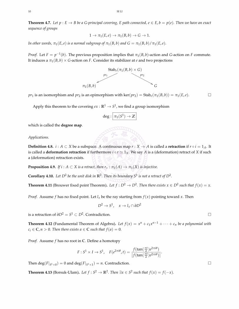
Proof. Let F = p−1(b). The previous proposition implies that π1(B, b)-action and G-action on F commute.It induces a π1(B, b)× G-action on F. Consider its stabilizer at e and two projections
Stabe(π1(B, b)× G)pr1
vv
pr2
''π1(B, b) G
pr1 is an isomorphism and pr2 is an epimorphism with ker(pr2) = Stabe(π1(B, b)) = π1(E, e).
Apply this theorem to the covering ex : R1 → S1, we find a group isomorphism
deg : π1(S1)→ Z
which is called the degree map.
Applications.
Definition 4.8. i : A ⊂ X be a subspace. A continuous map r : X → A is called a retraction if r i = 1A. Itis called a deformation retraction if furthermore i r ' 1X . We say A is a (deformation) retract of X if sucha (deformation) retraction exists.
Proposition 4.9. If i : A ⊂ X is a retract, then r∗ : π1(A)→ π1(X) is injective.
Corollary 4.10. Let D2 be the unit disk in R2. Then its boundary S1 is not a retract of D2.
Theorem 4.11 (Brouwer fixed point Theorem). Let f : D2 → D2. Then there exists x ∈ D2 such that f (x) = x.
Proof. Assume f has no fixed point. Let lx be the ray starting from f (x) pointing toward x. Then
D2 → S1, x → lx ∩ ∂D2
is a retraction of ∂D2 = S1 ⊂ D2. Contradiction.
Theorem 4.12 (Fundamental Theorem of Algebra). Let f (x) = xn + c1xn−1 + · · ·+ cn be a polynomial withci ∈ C, n > 0. Then there exists a ∈ C such that f (a) = 0.
Proof. Assume f has no root in C. Define a homotopy
F : S1 × I → S1, F(e2πiθ , t) =f (tan(πt
2 )e2πiθ)∣∣ f (tan(πt2 )e2πiθ)
∣∣ .Then deg(F|S1×0) = 0 and deg(F|S1×1) = n. Contradiction.
Theorem 4.13 (Borsuk-Ulam). Let f : S2 → R2. Then ∃x ∈ S2 such that f (x) = f (−x).
INTRODUCTION TO ALGEBRAIC TOPOLOGY 11
Proof. Assume f (x) 6= f (−x), ∀x ∈ S2. Define
ρ : S2 → S1, ρ(x) =f (x)− f (−x)| f (x)− f (−x)| .
Let D2 be the upper hemi-sphere of S2. It defines a homotopy between constant map and ρ|∂D2 : S1 → S1,hence deg(ρ|∂D2) = 0. On the other hand, ρ|∂D2 is antipode-preserving: ρ|∂D2(−x) = −ρ|∂D2(x), hencedeg(ρ|∂D2) is odd. Contradiction.
Corollary 4.14 (Ham Sandwich Theorem). Let A1, A2 be two bounded regions of positive areas in R2. Then thereexists a line which cuts each Ai into half of equal areas.
Proof. Let A1, A2 ⊂ R2 × 1 ⊂ R3. Given u ∈ S2, let Pu be the plane passing the origin and perpendicularto the unit vector u. Let Ai(u) = p ∈ Ai|p · u ≤ 0. Define the map
f : S2 → R2, fi(u) = Area(Ai(u)).
By Borsuk-Ulam, ∃u such that f (u) = f (−u). The intersection R2 × 1 ∩ Pu gives the required line.
5. CLASSIFICATION OF COVERING
Definition 5.1. The universal cover of B is a covering map p : E→ B with E simply connected.
Theorem 5.2. Assume B is path connected and locally path connected. Then universal cover of B exists if and onlyif B is semi-locally simply connected space.
Definition 5.3. We define the category Cov(B) of coverings of B
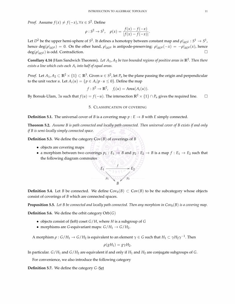
• objects are covering maps• a morphism between two coverings p1 : E1 → B and p2 : E2 → B is a map f : E1 → E2 such that
the following diagram commutes
E1f
//
p1
E2
p2B
Definition 5.4. Let B be connected. We define Cov0(B) ⊂ Cov(B) to be the subcategory whose objectsconsist of coverings of B which are connected spaces.
Proposition 5.5. Let B be connected and locally path connected. Then any morphism in Cov0(B) is a covering map.
Definition 5.6. We define the orbit category Orb(G)
• objects consist of (left) coset G/H, where H is a subgroup of G• morphisms are G-equivariant maps: G/H1 → G/H2.
A morphism ρ : G/H1 → G/H2 is equivalent to an element γ ∈ G such that H1 ⊂ γH2γ−1. Then
ρ(gH1) = gγH2.
In particular. G/H1 and G/H2 are equivalent if and only if H1 and H2 are conjugate subgroups of G.
For convenience, we also introduce the following category
Definition 5.7. We define the category G -Set
12 SI LI
• objects consist of sets with G-action• morphisms are G-equivariant set maps.
Given a covering p : E→ B, b ∈ B, we find
p−1(b) ∈ π1(B, b) -Set.
Proposition 5.8. Assume B is path connected and locally path connected. Let p1, p2 ∈ Cov(B). Then
HomCov(B)(p1, p2) ∼= Homπ1(B,b) -Set(p−11 (b), p−1
2 (b))
Proof. This is a consequence of Lifting Criterion and the Theorem of Uniqueness of lifting.
Definition 5.9. Let B be path connected and p : E → B be a connected covering. deck transformation (orcovering transformation) of p is a homeomorphism f : E → E such that p f = p. Let Aut(p) denote thegroup of deck transformation.
Note that Aut(p) acts freely on E by the Uniqueness of Lifting.
Proposition 5.10. Let B be path connected and p : E → B be a connected covering. Then Aut(p) acts properlydiscontinuous on E.
We find that the universal cover E is a π1(B, b)-principal covering.
Corollary 5.11. Assume B is path connected, locally path connected. Let p : E → B be a connected covering,e ∈ E, b = p(e) ∈ B, G = π1(B, b), H = π1(E, e). Then
Aut(p) ∼= NG(H)/H
where NG(H) is the normalizer of H in G.
Proof. By the above proposition,
Aut(p) ∼= HomG -Set(G/H, G/H) = NG(H)/H.
Theorem 5.12. Assume B is path connected, locally path connected and semi-locally simply connected. b ∈ B. Thenthere exists an equivalence of categories
Cov(B) ' π1(B, b) -Set .
Proof. Let us denote π1 = π1(B, b). Let p : B→ B be a fixed universal cover of B and b ∈ π−1(b) chosen.
We define the following functors
Cov(B)F --
π1 -Set.Gmm
Let p : E→ B be a covering, we defineF(p) = p−1(b).
Let S ∈ π1 -Set, we define
G(S) = B×π1 S = B× S/ ∼, where (e · g, s) ∼ (e, g · s), ∀e ∈ B, s ∈ S, g ∈ π1.
Here e · g represents the (right) π1-action on B. Then we have natural equivalences
F Gη' 1, G F
τ' 1.
INTRODUCTION TO ALGEBRAIC TOPOLOGY 13
Here η is the natural equivalence
ηS ∈ Homπ1 -Set(F G(S), S), ηS(e, s) = g · s if e = b · g.
τ is the natural equivalence
τE ∈ HomCov(B)(p′, p) ∼= Homπ1 -Set(p−1(b), p−1(b)), p′ : B×π1 p−1(b)→ B,
which is determined by the identity map in Homπ1 -Set(p−1(b), p−1(b)).
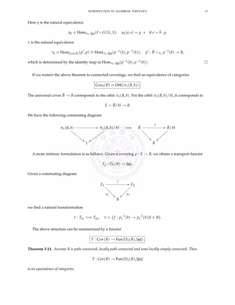
If we restrict the above theorem to connected coverings, we find an equivalence of categories
Cov0(B) ' Orb(π1(B, b)) .
The universal cover B→ B corresponds to the orbit π1(B, b). For the orbit π1(B, b)/H, it corresponds to
E = B/H → B.
We have the following commuting diagram
π1(B, b)
##
// π1(B, b)/H
zz1
=⇒ Bf
//
B/H
B
A more intrinsic formulation is as follows. Given a covering p : E→ B, we obtain a transport functor
Tp : Π1(B)→ Set .
Given a commuting diagram
E1f
//
p1
E2
p2B
we find a natural transformation
τ : Tp1 =⇒ Tp2 , τ = f : p−11 (b)→ p−1
2 (b)|b ∈ B.
The above structure can be summerized by a functor
T : Cov(B)→ Fun(Π1(B), Set) .
Theorem 5.13. Assume B is path connected, locally path connected and semi-locally simply connected. Then
T : Cov(B)→ Fun(Π1(B), Set)
is an equivalence of categories.
14 SI LI
6. SEIFERT-VAN KAMPEN THEOREM
Product.
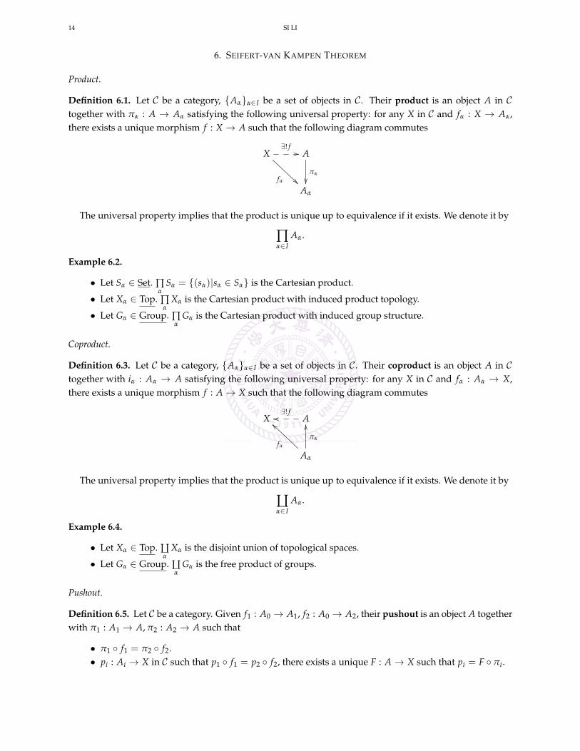
Definition 6.1. Let C be a category, Aαα∈I be a set of objects in C. Their product is an object A in Ctogether with πα : A → Aα satisfying the following universal property: for any X in C and fα : X → Aα,there exists a unique morphism f : X → A such that the following diagram commutes
X∃! f//
fα
A
πα
Aα
The universal property implies that the product is unique up to equivalence if it exists. We denote it by
∏α∈I
Aα.
Example 6.2.
• Let Sα ∈ Set. ∏α
Sα = (sα)|sα ∈ Sα is the Cartesian product.
• Let Xα ∈ Top. ∏α
Xα is the Cartesian product with induced product topology.
• Let Gα ∈ Group. ∏α
Gα is the Cartesian product with induced group structure.
Coproduct.
Definition 6.3. Let C be a category, Aαα∈I be a set of objects in C. Their coproduct is an object A in Ctogether with iα : Aα → A satisfying the following universal property: for any X in C and fα : Aα → X,there exists a unique morphism f : A→ X such that the following diagram commutes
X A∃! foo
Aα
πα
OO
fα
``
The universal property implies that the product is unique up to equivalence if it exists. We denote it by
äα∈I
Aα.
Example 6.4.
• Let Xα ∈ Top. äα
Xα is the disjoint union of topological spaces.
• Let Gα ∈ Group. äα
Gα is the free product of groups.
Pushout.
Definition 6.5. Let C be a category. Given f1 : A0 → A1, f2 : A0 → A2, their pushout is an object A togetherwith π1 : A1 → A, π2 : A2 → A such that
• π1 f1 = π2 f2.• pi : Ai → X in C such that p1 f1 = p2 f2, there exists a unique F : A→ X such that pi = F πi.
INTRODUCTION TO ALGEBRAIC TOPOLOGY 15
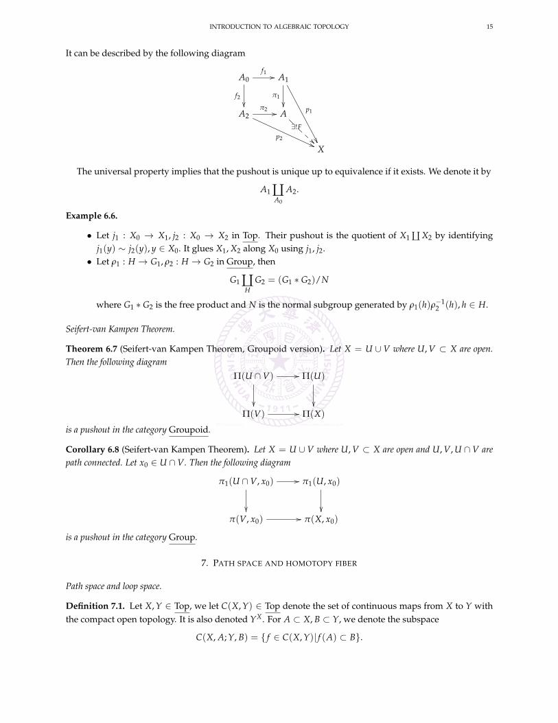
It can be described by the following diagram
A0f1 //
f2
A1
π1
p1
A2
p2((
π2 // A∃!F
X
The universal property implies that the pushout is unique up to equivalence if it exists. We denote it by
A1 äA0
A2.
Example 6.6.
• Let j1 : X0 → X1, j2 : X0 → X2 in Top. Their pushout is the quotient of X1 ä X2 by identifyingj1(y) ∼ j2(y), y ∈ X0. It glues X1, X2 along X0 using j1, j2.
• Let ρ1 : H → G1, ρ2 : H → G2 in Group, then
G1 äH
G2 = (G1 ∗ G2)/N
where G1 ∗ G2 is the free product and N is the normal subgroup generated by ρ1(h)ρ−12 (h), h ∈ H.
Seifert-van Kampen Theorem.
Theorem 6.7 (Seifert-van Kampen Theorem, Groupoid version). Let X = U ∪ V where U, V ⊂ X are open.Then the following diagram
Π(U ∩V) //
Π(U)
Π(V) // Π(X)
is a pushout in the category Groupoid.
Corollary 6.8 (Seifert-van Kampen Theorem). Let X = U ∪ V where U, V ⊂ X are open and U, V, U ∩ V arepath connected. Let x0 ∈ U ∩V. Then the following diagram
π1(U ∩V, x0) //
π1(U, x0)
π(V, x0) // π(X, x0)
is a pushout in the category Group.
7. PATH SPACE AND HOMOTOPY FIBER
Path space and loop space.
Definition 7.1. Let X, Y ∈ Top, we let C(X, Y) ∈ Top denote the set of continuous maps from X to Y withthe compact open topology. It is also denoted YX . For A ⊂ X, B ⊂ Y, we denote the subspace
C(X, A; Y, B) = f ∈ C(X, Y)| f (A) ⊂ B.
16 SI LI
Theorem 7.2 (Exponential Correspondence). Let Y be locally compact Hausdorff. Then the evaluation mapC(Y, Z)×Y → Z is continuous and we have
HomTop(X×Y, Z) = HomTop(X, C(Y, Z)).
If furthermore X is Hausdorff, then
C(X×Y, Z) = C(X, C(Y, Z)).
Definition 7.3. Let X ∈ Top, we define
• free path space PX = C(I, X) and based path space PxX = C(I, 0; X, x);• free loop space LX = C(S1, X) and based loop space ΩxX = C(S1, 1; X, x) or simply ΩX.
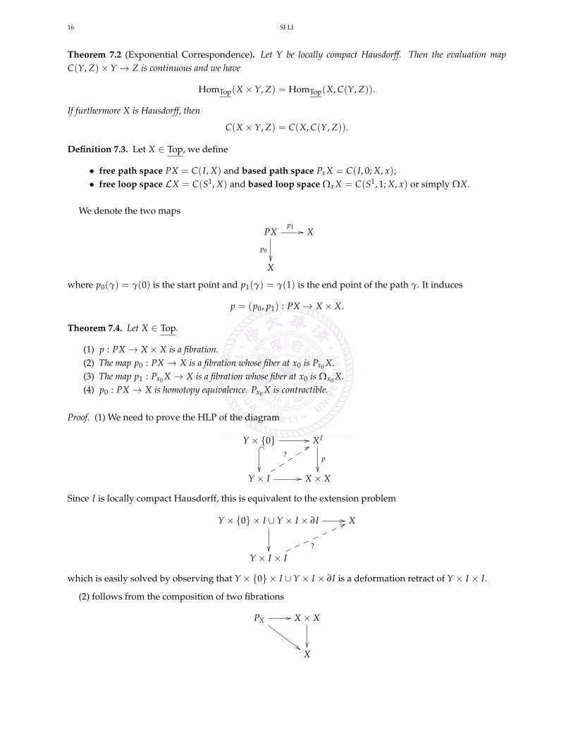
We denote the two maps
PXp1 //
p0
X
X
where p0(γ) = γ(0) is the start point and p1(γ) = γ(1) is the end point of the path γ. It induces
p = (p0, p1) : PX → X× X.
Theorem 7.4. Let X ∈ Top.
(1) p : PX → X× X is a fibration.(2) The map p0 : PX → X is a fibration whose fiber at x0 is Px0 X.(3) The map p1 : Px0 X → X is a fibration whose fiber at x0 is Ωx0 X.(4) p0 : PX → X is homotopy equivalence. Px0 X is contractible.
Proof. (1) We need to prove the HLP of the diagram
Y× 0 // _
X I
p
Y× I //
?99
X× X
Since I is locally compact Hausdorff, this is equivalent to the extension problem
Y× 0 × I ∪Y× I × ∂I //
X
Y× I × I?
66
which is easily solved by observing that Y× 0 × I ∪Y× I × ∂I is a deformation retract of Y× I × I.
(2) follows from the composition of two fibrations
PX //
##
X× X
X
INTRODUCTION TO ALGEBRAIC TOPOLOGY 17
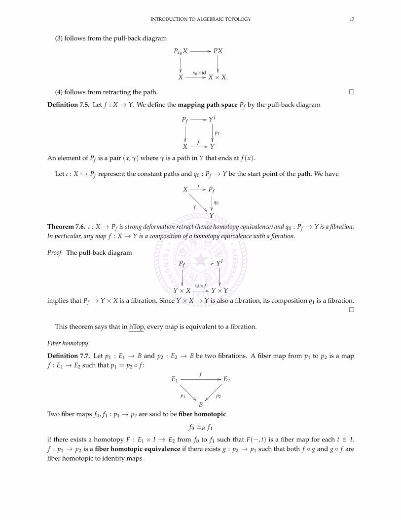
(3) follows from the pull-back diagram
Px0 X
// PX
X
x0×id// X× X.
(4) follows from retracting the path.
Definition 7.5. Let f : X → Y. We define the mapping path space Pf by the pull-back diagram
Pf //
Y I
p1
X
f// Y
An element of Pf is a pair (x, γ) where γ is a path in Y that ends at f (x).
Let ι : X → Pf represent the constant paths and q0 : Pf → Y be the start point of the path. We have
X ι //
f
Pf
q0
Y
Theorem 7.6. ι : X → Pf is strong deformation retract (hence homotopy equivalence) and q0 : Pf → Y is a fibration.In particular, any map f : X → Y is a composition of a homotopy equivalence with a fibration.
Proof. The pull-back diagram
Pf
// Y I
Y× X
id× f// Y×Y
implies that Pf → Y× X is a fibration. Since Y× X → Y is also a fibration, its composition q1 is a fibration.
This theorem says that in hTop, every map is equivalent to a fibration.
Fiber homotopy.
Definition 7.7. Let p1 : E1 → B and p2 : E2 → B be two fibrations. A fiber map from p1 to p2 is a mapf : E1 → E2 such that p1 = p2 f :
E1
p1
f// E2
p2B
Two fiber maps f0, f1 : p1 → p2 are said to be fiber homotopic
f0 'B f1
if there exists a homotopy F : E1 × I → E2 from f0 to f1 such that F(−, t) is a fiber map for each t ∈ I.f : p1 → p2 is a fiber homotopic equivalence if there exists g : p2 → p1 such that both f g and g f arefiber homotopic to identity maps.
18 SI LI
Proposition 7.8. Let p1 : E1 → B and p2 : E2 → B be two fibrations and f : E1 → E2 be a fiber map. Assumef : E1 → E2 is a homotopy equivalence, then f is a fiber homotopy equivalence. In particular, f : p−1
1 (b)→ p−12 (b)
is a homotopy equivalence for any b ∈ B.
Proof. We only need to prove that for any fiber map f : E1 → E2 which is a homotopy equivalence, there isa fiber map g : E2 → E1 such that g f 'B 1. In fact, such a g is also a homotopy equivalence and we canfind h : E1 → E2 such that h g 'B 1. Then f 'B h g f 'B h, which implies f g 'B 1 as well.
Let g : E2 → E1 be a homotopy inverse of f , so g = f−1 in hTop. We first show that we can choose ahomotopy class of g such that g is a fiber map. In fact, consider the diagram
E1
p1
E2
p1g&&
p2
88
g>>
B
Since g p1 = g f p2 is homotopic to p2 and p1 is a fibration, we can lift the above homotopy to ahomotopy from g to g′ : E2 → E1 which lifts p2. Then g′ is a fiber map as required.
We further reduce the problem to prove the following
“Claim”: Let p : E → B be a fibration and f : E → E is a fiber map that is homotopic to 1E, then there is afiber map h : E→ E such that h f 'B 1.
In fact, let f : E1 → E2 as in the proposition, g : E2 → E1 be a fiber map such that g f ' 1 as chosenabove. The “Claim” implies that we can find a fiber map h : E1 → E1 such that h g f 'B 1. The the fibermap g = h g has the required property that g f 'B 1.
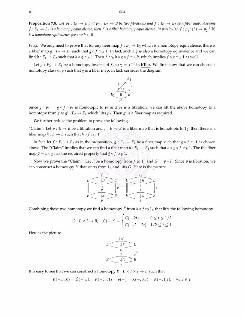
Now we prove the “Claim”. Let F be a homotopy from f to 1E and G = p F. Since p is fibration, wecan construct a homotopy H that starts from 1E and lifts G. Here is the picture
Ef
))
1E
55 F E
p
Ep
))
p55 G B
E1E
))
h
55 H E
p
Ep
))
p55 G B
Combining these two homotopy we find a homotopy F from h f to 1E that lifts the following homotopy
G : E× I → B, G(−, t) =
G(−.2t) 0 ≤ t ≤ 1/2
G(−, 2− 2t) 1/2 ≤ t ≤ 1
Here is the picture
Eh f
))
1E
55 F E
p
Ep
))
p55 G B
It is easy to see that we can construct a homotopy K : E× I × I → B such that
K(−, u, 0) = G(−, u), K(−, u, 1) = p(−) = K(−, 0, t) = K(−, 1, t), ∀u, t ∈ I.
INTRODUCTION TO ALGEBRAIC TOPOLOGY 19
Since p is a fibration, we can find a lift K : E× I × I → E of K such that
K(−, u, 0) = F(−, u).
Then we have the following fiber homotopy
h f = K(−, 0, 0) 'B K(−, 0, 1) 'B K(−, 1, 1) 'B K(−, 1, 0) = 1E.
Homotopy fiber.
Definition 7.9. Let f : X → Y, we define its homotopy fiber over y ∈ Y to be the fiber of Pf → Y over y.
If Y is path connected, then all homotopy fibers are homotopic equivalent since Pf → Y is a fibration. Inthis case we will usually write the following diagram
F // X
f
Y
where F denotes the homotopy fiber.
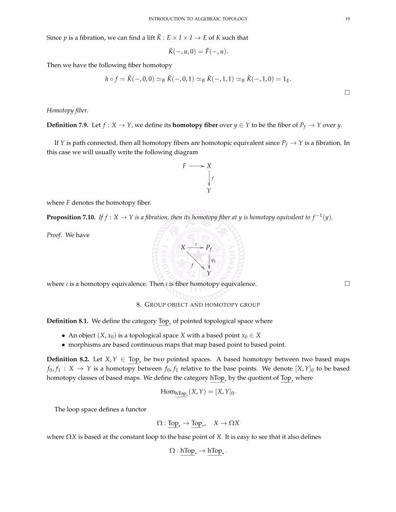
Proposition 7.10. If f : X → Y is a fibration, then its homotopy fiber at y is homotopy equivalent to f−1(y).
Proof. We have
X ι //
f
Pf
q1
Y
where ι is a homotopy equivalence. Then ι is fiber homotopy equivalence.
8. GROUP OBJECT AND HOMOTOPY GROUP
Definition 8.1. We define the category Top*
of pointed topological space where
• An object (X, x0) is a topological space X with a based point x0 ∈ X• morphisms are based continuous maps that map based point to based point.
Definition 8.2. Let X, Y ∈ Top*
be two pointed spaces. A based homotopy between two based mapsf0, f1 : X → Y is a homotopy between f0, f1 relative to the base points. We denote [X, Y]0 to be basedhomotopy classes of based maps. We define the category hTop
*by the quotient of Top
*where
HomhTop*(X, Y) = [X, Y]0.
The loop space defines a functor
Ω : Top*→ Top
*, X → ΩX
where ΩX is based at the constant loop to the base point of X. It is easy to see that it also defines
Ω : hTop*→ hTop
*.
20 SI LI
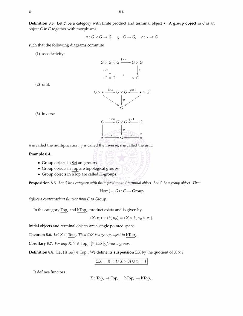
Definition 8.3. Let C be a category with finite product and terminal object ?. A group object in C is anobject G in C together with morphisms
µ : G× G → G, η : G → G, ε : ?→ G
such that the following diagrams commute
(1) associativity:
G× G× G1×µ
//
µ×1
G× G
µ
G× G
µ// G
(2) unit:
G× ?1×ε //
$$
G× G
µ
?× Gε×1oo
zzG
(3) inverse
G
1×η// G× G
µ
Gη×1oo
?
ε // G ?εoo
µ is called the multiplication, η is called the inverse, ε is called the unit.
Example 8.4.
• Group objects in Set are groups.• Group objects in Top are topological groups.• Group objects in hTop are called H-groups.
Proposition 8.5. Let C be a category with finite product and terminal object. Let G be a group object. Then
Hom(−, G) : C → Group
defines a contravariant functor from C to Group.
In the category Top*
and hTop*, product exists and is given by
(X, x0)× (Y, y0) = (X×Y, x0 × y0).
Initial objects and terminal objects are a single pointed space.
Theorem 8.6. Let X ∈ Top*. Then ΩX is a group object in hTop
*.
Corollary 8.7. For any X, Y ∈ Top*, [Y, ΩX]0 forms a group.
Definition 8.8. Let (X, x0) ∈ Top*. We define its suspension ΣX by the quotient of X× I
ΣX = X× I/X× ∂I ∪ x0 × I .
It defines functorsΣ : Top
*→ Top
*, hTop
*→ hTop
*.
INTRODUCTION TO ALGEBRAIC TOPOLOGY 21
Example 8.9. ΣSn ∼= Sn+1 are homeomorphic for any n ≥ 0.
Definition 8.10. Let F : C → D and G : D → C be two functors. (F, G) is called adjoint pair if there areisomorphisms
τ : HomD(FX, Y) ∼= HomC(X, GY), ∀X ∈ C, Y ∈ Dwhich are natural for all X, Y. In other words, τ defines a natural equivalence between two functors
HomD(F−,−), HomC(−, G−) : Cop ×D → Set .
F (G) is called the left (right) adjoint of G (F), denoted by F a G.
Example 8.11. Let Y be locally compat Hausdorff, then −×Y is left adjoint to C(Y,−).
Proposition 8.12. (Σ, Ω) is an adjoint pair in Top*
and hTop*.
Definition 8.13. Let (X, x0) ∈ Top*. We define the n-th homotopy group
πn(X, x0) = [Sn, X]0 .
Sometimes we simply denote it by πn(X).
For n ≥ 1, we know thatπn(X) = [ΣSn−1, X]0 = [Sn−1, ΩX]
which is a group since ΩX is a group object.
Proposition 8.14. πn(X) is abelian if n ≥ 2.
Proposition 8.15. Let X be path connected. There is a natural functor
T : Π1(X)→ Group
which sends x0 to πn(X, x0). In particular, there is a natural action of π1(X, x0) on πn(X, x0) and all πn(X, x0)’sare isomorphic for different choices of x0.
Proposition 8.16. Let f : X → Y be homotopy equivalence. Then
f∗ : πn(X, x0)→ πn(Y, f (x0))
is a group isomorphism.
9. EXACT PUPPE SEQUENCE
Definition 9.1. A sequence of maps of sets with base points
(A, a0)f→ (B, b0)
g→ (C, c0)
is said to be exact at B if im( f ) = ker(g) where im( f ) = f (A), ker(g) = g−1(c0). A sequence
· · · → An+1 → An → An−1 → · · ·
is called an exact sequence if it is exact at every Ai.
Definition 9.2. A sequence of maps in hTop*
· · · → Xn+1 → Xn → Xn−1 → · · ·
is called exact if for any Y ∈ hTop*, the following sequence of pointed sets is exact
· · · → [Y, Xn+1]0 → [Y, Xn]0 → [Y, Xn−1]0 → · · ·
22 SI LI
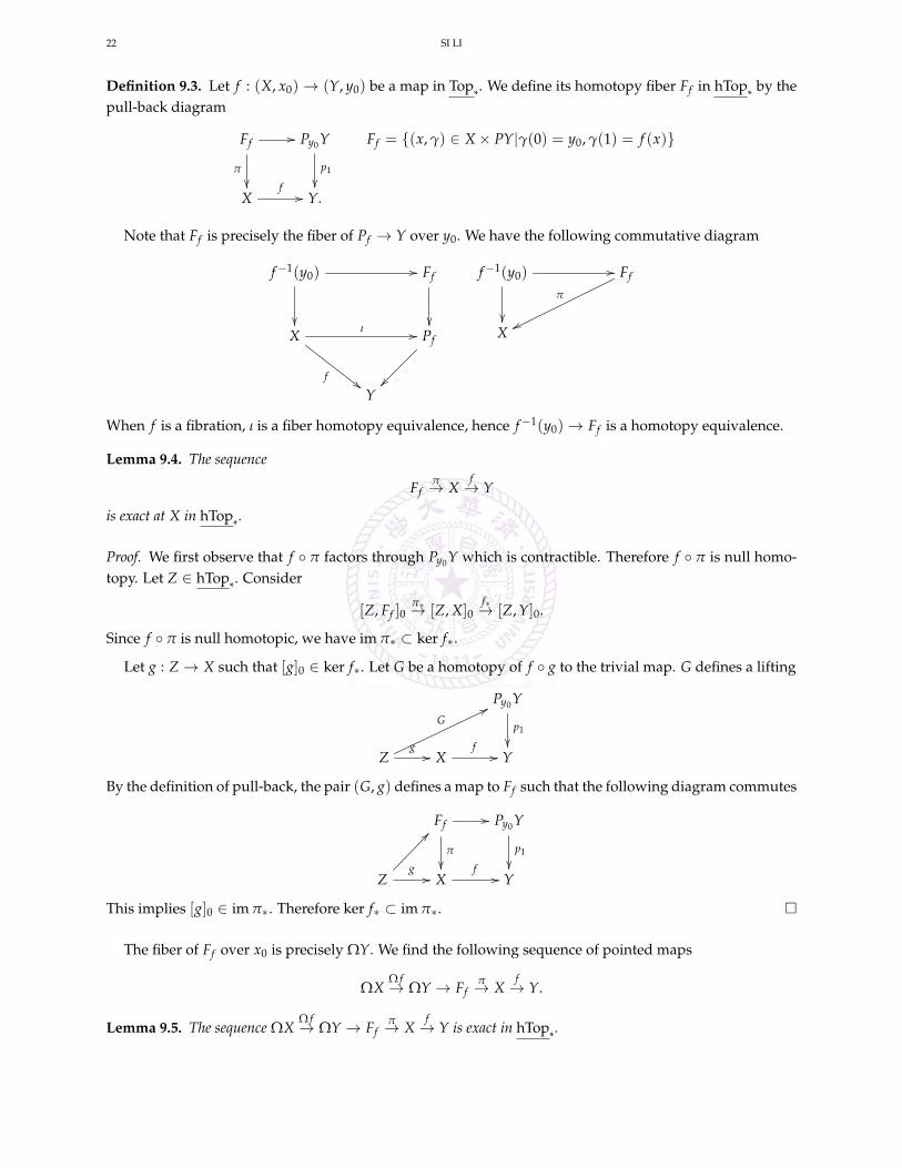
Definition 9.3. Let f : (X, x0)→ (Y, y0) be a map in Top*. We define its homotopy fiber Ff in hTop
*by the
pull-back diagram
Ff //
π
Py0Y
p1
X
f// Y.
Ff = (x, γ) ∈ X× PY|γ(0) = y0, γ(1) = f (x)
Note that Ff is precisely the fiber of Pf → Y over y0. We have the following commutative diagram
f−1(y0) //
Ff
X ι //
f##
Pf
Y
f−1(y0) //
Ff
π
wwX
When f is a fibration, ι is a fiber homotopy equivalence, hence f−1(y0)→ Ff is a homotopy equivalence.
Lemma 9.4. The sequence
Ffπ→ X
f→ Y
is exact at X in hTop*.
Proof. We first observe that f π factors through Py0Y which is contractible. Therefore f π is null homo-topy. Let Z ∈ hTop
*. Consider
[Z, Ff ]0π∗→ [Z, X]0
f∗→ [Z, Y]0.
Since f π is null homotopic, we have im π∗ ⊂ ker f∗.
Let g : Z → X such that [g]0 ∈ ker f∗. Let G be a homotopy of f g to the trivial map. G defines a lifting
Py0Y
p1
Z
g//
G77
Xf// Y
By the definition of pull-back, the pair (G, g) defines a map to Ff such that the following diagram commutes
Ff //
π
Py0Y
p1
Z
g//
??
Xf// Y
This implies [g]0 ∈ im π∗. Therefore ker f∗ ⊂ im π∗.
The fiber of Ff over x0 is precisely ΩY. We find the following sequence of pointed maps
ΩXΩ f→ ΩY → Ff
π→ Xf→ Y.
Lemma 9.5. The sequence ΩXΩ f→ ΩY → Ff
π→ Xf→ Y is exact in hTop
*.
INTRODUCTION TO ALGEBRAIC TOPOLOGY 23
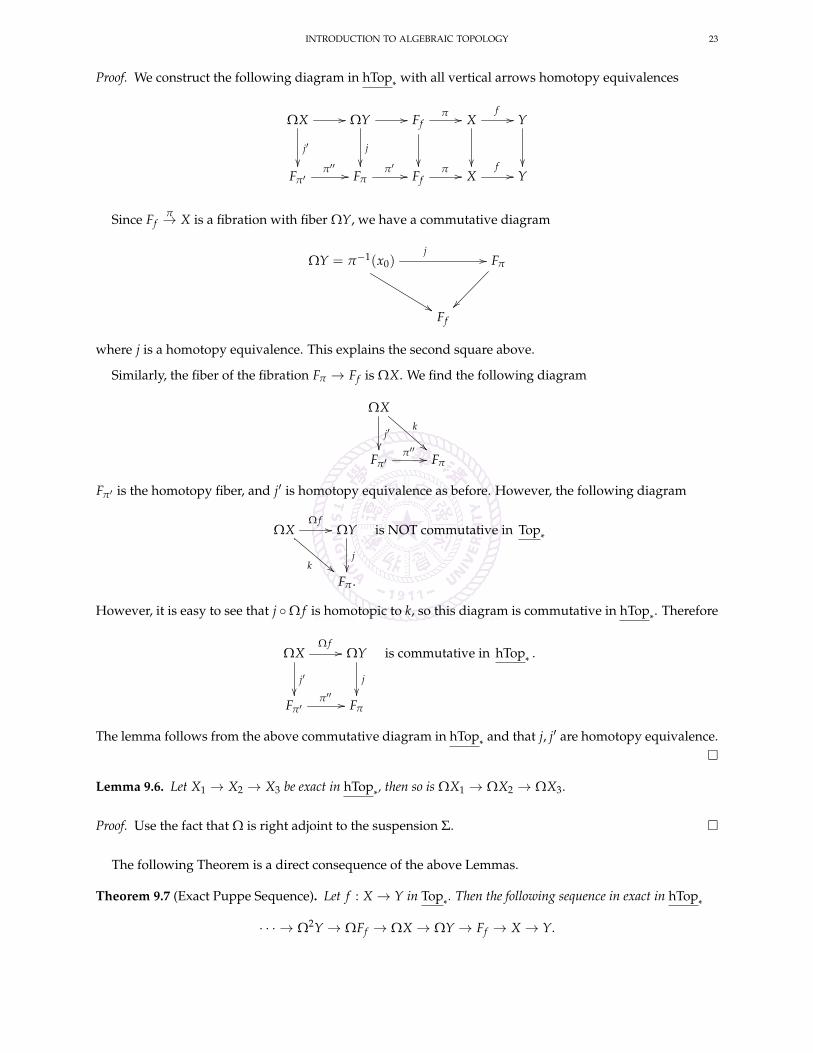
Proof. We construct the following diagram in hTop*
with all vertical arrows homotopy equivalences
ΩX //
j′
ΩY //
j
Ffπ //
Xf//
Y
Fπ′
π′′ // Fππ′ // Ff
π // Xf// Y
Since Ffπ→ X is a fibration with fiber ΩY, we have a commutative diagram
ΩY = π−1(x0)j
//
%%
Fπ
Ff
where j is a homotopy equivalence. This explains the second square above.
Similarly, the fiber of the fibration Fπ → Ff is ΩX. We find the following diagram
ΩX
j′
k
!!Fπ′
π′′ // Fπ
Fπ′ is the homotopy fiber, and j′ is homotopy equivalence as before. However, the following diagram
ΩX
k ""
Ω f// ΩY
j
Fπ .
is NOT commutative in Top*
However, it is easy to see that j Ω f is homotopic to k, so this diagram is commutative in hTop*. Therefore
ΩX
j′
Ω f// ΩY
j
Fπ′π′′ // Fπ
is commutative in hTop*
.
The lemma follows from the above commutative diagram in hTop*
and that j, j′ are homotopy equivalence.
Lemma 9.6. Let X1 → X2 → X3 be exact in hTop*, then so is ΩX1 → ΩX2 → ΩX3.
Proof. Use the fact that Ω is right adjoint to the suspension Σ.
The following Theorem is a direct consequence of the above Lemmas.
Theorem 9.7 (Exact Puppe Sequence). Let f : X → Y in Top*. Then the following sequence in exact in hTop
*
· · · → Ω2Y → ΩFf → ΩX → ΩY → Ff → X → Y.
24 SI LI
Theorem 9.8. Let π : E→ B be a map in Top*. Assume π is fibration whose fiber over the base point is F. Then we
have the following exact sequence of homotopy groups
· · · → πn(F)→ πn(E)→ πn(B)→ πn−1(F)→ · · · → π0(E)→ π0(B)
where all homotopy groups are understood to have based points on the relevant spaces.
Proof. Since π is a fibration, F is homotopy equivalent to Fπ . Apply [S0,−] to the Puppe Sequence.
The following proposition gives a criterion for fibration
Theorem 9.9. Let p : E → B with B paracompact Hausdorff. Assume there exists an open cover Uα of B suchthat p−1(Uα)→ Uα is a fibration. Then p is a fibration.
Corollary 9.10. Let p : E→ B be a fiber bundle with B paracompact Hausdorff. Then p is a fibration.
Proposition 9.11. If i < n, then πi(Sn) = 0.
Example 9.12. We have the Hopf fibration S3 → S2 with fiber S1. Its associated exact sequence of homotopygroups implies
π2(S2) ∼= Z, πn(S3) ∼= πn(S2) for n ≥ 3.
10. COFIBRATION
Cofibration.
Definition 10.1. A map i : A → X is said to have the homotopy extension property (HEP) with respect toY if for any maps f : X → Y and F : A → Y I such that p0 F = f i, there exists a map F : X → Y I suchthat the following diagram commutes
Y Xf
oo
∃F
~~Y I
p0
OO
A
i
OO
Foo
Definition 10.2. A map i : A→ X is called a cofibration if it has HEP for any spaces.
The notion of cofibration is dual to that of the fibration. Fibration is defined by the HLP of the diagram
Yf// _
E
p
Y× IF//
∃F<<
B
If we reverse the arrows and observe that Y × I is dual to the path space Y I via the adjointness of (−)× Iand (−)I , we arrive at HEP.
INTRODUCTION TO ALGEBRAIC TOPOLOGY 25
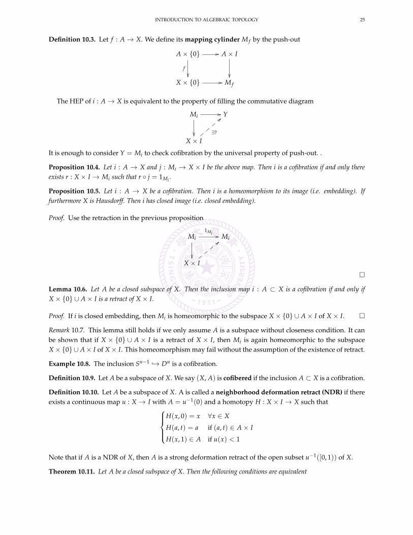
Definition 10.3. Let f : A→ X. We define its mapping cylinder M f by the push-out
A× 0
f
// A× I
X× 0 // M f
The HEP of i : A→ X is equivalent to the property of filling the commutative diagram
Mi
// Y
X× I∃?
==
It is enough to consider Y = Mi to check cofibration by the universal property of push-out. .
Proposition 10.4. Let i : A → X and j : Mi → X × I be the above map. Then i is a cofibration if and only thereexists r : X× I → Mi such that r j = 1Mi .
Proposition 10.5. Let i : A → X be a cofibration. Then i is a homeomorphism to its image (i.e. embedding). Iffurthermore X is Hausdorff. Then i has closed image (i.e. closed embedding).
Proof. Use the retraction in the previous proposition
Mi
1Mi // Mi
X× I
<<
Lemma 10.6. Let A be a closed subspace of X. Then the inclusion map i : A ⊂ X is a cofibration if and only ifX× 0 ∪ A× I is a retract of X× I.
Proof. If i is closed embedding, then Mi is homeomorphic to the subspace X× 0 ∪ A× I of X× I.
Remark 10.7. This lemma still holds if we only assume A is a subspace without closeness condition. It canbe shown that if X × 0 ∪ A × I is a retract of X × I, then Mi is again homeomorphic to the subspaceX×0 ∪ A× I of X× I. This homeomorphism may fail without the assumption of the existence of retract.
Example 10.8. The inclusion Sn−1 → Dn is a cofibration.
Definition 10.9. Let A be a subspace of X. We say (X, A) is cofibered if the inclusion A ⊂ X is a cofibration.
Definition 10.10. Let A be a subspace of X. A is called a neighborhood deformation retract (NDR) if thereexists a continuous map u : X → I with A = u−1(0) and a homotopy H : X× I → X such that
H(x, 0) = x ∀x ∈ X
H(a, t) = a if (a, t) ∈ A× I
H(x, 1) ∈ A if u(x) < 1
Note that if A is a NDR of X, then A is a strong deformation retract of the open subset u−1([0, 1)) of X.
Theorem 10.11. Let A be a closed subspace of X. Then the following conditions are equivalent
26 SI LI
(1) (X, A) is a cofibered pair.(2) A is a NDR of X.(3) X× 0 ∪ A× I is a retract of X× I.(4) X× 0 ∪ A× I is a strong deformation retract of X× I.
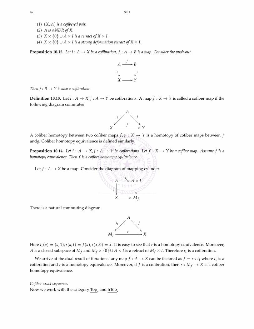
Proposition 10.12. Let i : A→ X be a cofibration, f : A→ B is a map. Consider the push-out
A
i
f// B
j
X // Y
Then j : B→ Y is also a cofibration.
Definition 10.13. Let i : A → X, j : A → Y be cofibrations. A map f : X → Y is called a cofiber map if thefollowing diagram commutes
Ai
j
X
f// Y
A cofiber homotopy between two cofiber maps f , g : X → Y is a homotopy of cofiber maps between fandg. Cofiber homotopy equivalence is defined similarly.
Proposition 10.14. Let i : A → X, j : A → Y be cofibrations. Let f : X → Y be a cofiber map. Assume f is ahomotopy equivalence. Then f is a cofiber homotopy equivalence.
Let f : A→ X be a map. Consider the diagram of mapping cylinder
A
f
i0 // A× I
X // M f
There is a natural commuting diagram
Ai1
~~
f
M f
r // X
Here i1(a) = (a, 1), r(a, t) = f (a), r(x, 0) = x. It is easy to see that r is a homotopy equivalence. Moreover,A is a closed subspace of M f and M f × 0 ∪ A× I is a retract of M f × I. Therefore i1 is a cofibration.
We arrive at the dual result of fibrations: any map f : A → X can be factored as f = r i1 where i1 is acofibration and r is a homotopy equivalence. Moreover, if f is a cofibration, then r : M f → X is a cofiberhomotopy equivalence.
Cofiber exact sequence.Now we work with the category Top
*and hTop
*.
INTRODUCTION TO ALGEBRAIC TOPOLOGY 27
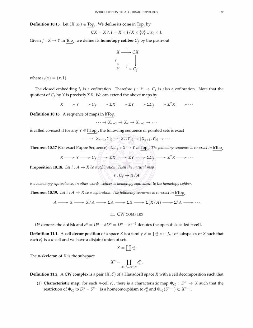
Definition 10.15. Let (X, x0) ∈ Top*. We define its cone in Top
*by
CX = X ∧ I = X× I/X× 0 ∪ x0 × I.
Given f : X → Y in Top*, we define its homotopy cofiber C f by the push-out
X
f
i1 // CX
Y
j// C f
where i1(x) = (x, 1).
The closed embedding i1 is a cofibration. Therefore j : Y → C f is also a cofibration. Note that thequotient of C f by Y is precisely ΣX. We can extend the above maps by
X // Y // C f // ΣX // ΣY // ΣC f // Σ2X // · · ·
Definition 10.16. A sequence of maps in hTop*
· · · → Xn+1 → Xn → Xn−1 → · · ·
is called co-exact if for any Y ∈ hTop*, the following sequence of pointed sets is exact
· · · → [Xn−1, Y]0 → [Xn, Y]0 → [Xn+1, Y]0 → · · ·
Theorem 10.17 (Co-exact Puppe Sequence). Let f : X → Y in Top*. The following sequence is co-exact in hTop
*
X // Y // C f // ΣX // ΣY // ΣC f // Σ2X // · · ·
Proposition 10.18. Let i : A→ X be a cofibration. Then the natural map
r : C f → X/A
is a homotopy equivalence. In other words, cofiber is homotopy equivalent to the homotopy cofiber.
Theorem 10.19. Let i : A→ X be a cofibration. The following sequence is co-exact in hTop*
A // X // X/A // ΣA // ΣX // Σ(X/A) // Σ2 A // · · ·
11. CW COMPLEX
Dn denotes the n-disk and en = Dn − ∂Dn = Dn − Sn−1 denotes the open disk called n-cell.
Definition 11.1. A cell decomposition of a space X is a family E = enα |α ∈ Jn of subspaces of X such that
each enα is a n-cell and we have a disjoint union of sets
X = ä enα .
The n-skeleton of X is the subspaceXn = ä
α∈Jm ,m≤nem
α .
Definition 11.2. A CW complex is a pair (X, E) of a Hausdorff space X with a cell decomposition such that
(1) Characteristic map: for each n-cell enα , there is a characteristic map Φen
α: Dn → X such that the
restriction of Φeαn to Dn − Sn−1 is a homeomorphism to en
α and Φenα(Sn−1) ⊂ Xn−1.
28 SI LI
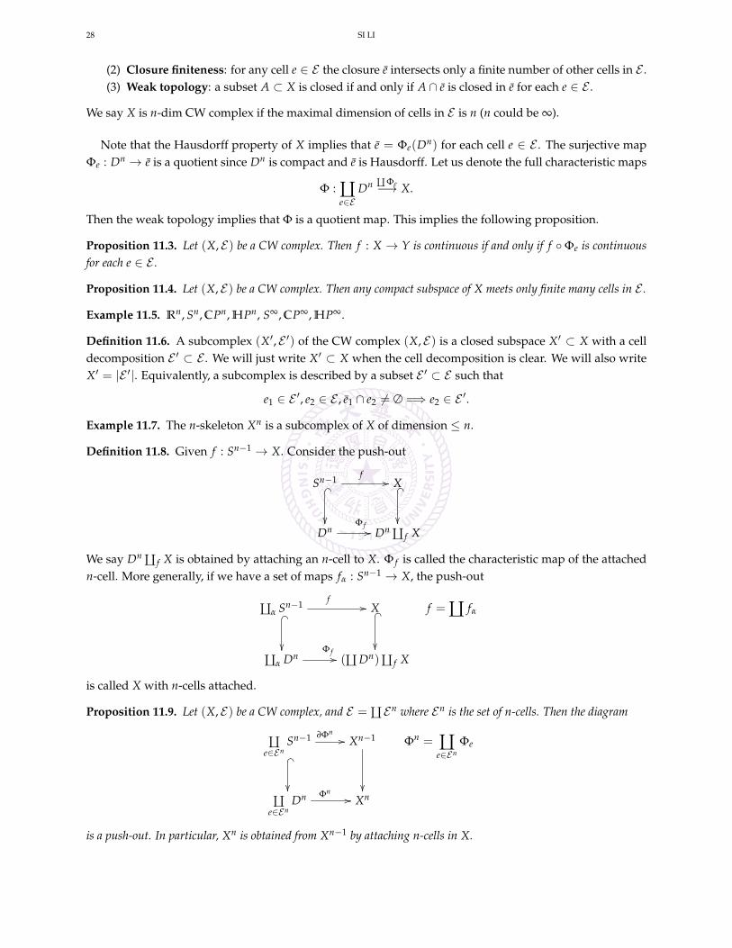
(2) Closure finiteness: for any cell e ∈ E the closure e intersects only a finite number of other cells in E .(3) Weak topology: a subset A ⊂ X is closed if and only if A ∩ e is closed in e for each e ∈ E .
We say X is n-dim CW complex if the maximal dimension of cells in E is n (n could be ∞).
Note that the Hausdorff property of X implies that e = Φe(Dn) for each cell e ∈ E . The surjective mapΦe : Dn → e is a quotient since Dn is compact and e is Hausdorff. Let us denote the full characteristic maps
Φ : äe∈E
Dn ä Φe−→ X.
Then the weak topology implies that Φ is a quotient map. This implies the following proposition.
Proposition 11.3. Let (X, E) be a CW complex. Then f : X → Y is continuous if and only if f Φe is continuousfor each e ∈ E .
Proposition 11.4. Let (X, E) be a CW complex. Then any compact subspace of X meets only finite many cells in E .
Example 11.5. Rn, Sn, CPn, HPn, S∞, CP∞, HP∞.
Definition 11.6. A subcomplex (X′, E ′) of the CW complex (X, E) is a closed subspace X′ ⊂ X with a celldecomposition E ′ ⊂ E . We will just write X′ ⊂ X when the cell decomposition is clear. We will also writeX′ = |E ′|. Equivalently, a subcomplex is described by a subset E ′ ⊂ E such that
e1 ∈ E ′, e2 ∈ E , e1 ∩ e2 6= ∅ =⇒ e2 ∈ E ′.
Example 11.7. The n-skeleton Xn is a subcomplex of X of dimension ≤ n.
Definition 11.8. Given f : Sn−1 → X. Consider the push-out
Sn−1 f//
_
X _
Dn
Φ f // Dn ä f X
We say Dn ä f X is obtained by attaching an n-cell to X. Φ f is called the characteristic map of the attachedn-cell. More generally, if we have a set of maps fα : Sn−1 → X, the push-out
äα Sn−1 f//
_
X _
äα Dn
Φ f // (ä Dn)ä f X
f = ä fα
is called X with n-cells attached.
Proposition 11.9. Let (X, E) be a CW complex, and E = ä En where En is the set of n-cells. Then the diagram
äe∈En
Sn−1 ∂Φn//
_
Xn−1
ä
e∈EnDn Φn
// Xn
Φn = äe∈En
Φe
is a push-out. In particular, Xn is obtained from Xn−1 by attaching n-cells in X.
INTRODUCTION TO ALGEBRAIC TOPOLOGY 29
Proof. This follows from the fact that Xn−1 is a closed subspace of Xn and the weak topology.
The converse is also true. The next proposition can be viewed as an alternate definition of CW complex.
Proposition 11.10. Suppose we have a sequence of spaces
∅ = X−1 ⊂ X0 ⊂ X1 ⊂ · · · ⊂ Xn ⊂ Xn+1 ⊂ · · ·
where Xn is obtained from Xn−1 by attaching n-cells. Let X = ∪n≥0Xn be the union with the weak topology: A ⊂ Xis closed if and only if A ∩ Xn is closed in Xn for each n. Then X is a CW complex.
Proof. The nontrivial part is to show that X is Hausdorff.
Definition 11.11. Let A be a subspace of X. A CW decomposition of (X, A) consiss of a sequence
A = X−1 ⊂ X0 ⊂ X1 ⊂ · · · ⊂ X
such that Xn is obtained from Xn−1 by attaching n-cells and X carries the weak topology with respect to thesubspaces Xn. The pair (X, A) is called a relative CW complex.
Note that for a relative CW complex (X, A), A itself may not have any cell structures.
Proposition 11.12. Let (X, A) be a relative CW complex. Then A ⊂ X is a cofibration.
Proof. Sn−1 → Dn is a cofibration, and cofibration is preserved under push-out and compositions.
Corollary 11.13. Let X be a CW complex and X′ be a CW subcomplex. Then X′ → X is a cofibration.
Proof. (X, X′) is a relative CW complex.
Proposition 11.14. Let X.Y be CW complexes. X is locally compact. Then X×Y is a CW complex
12. WHITEHEAD THEOREM
Relative homotopy group.
Definition 12.1. The define the category TopP of topological pairs where an object (X, A) is a topologicalspace X with a subspace X, and morphisms (X, A) → (Y, B) are continuous maps f : X → Y such thatf (A) ⊂ B. A homotopy between two maps f1, f2 : (X, A) → (Y, B) is a homotopy F : X × I → Y betweenf0, f1 such that F|X×t(A) ⊂ B for any t ∈ I.
The quotient category of TopP by homotopy of maps is denoted by hTopP. The pointed versions aredefined similarly and denoted by TopP
*and hTopP
*. Morphisms in hTopP and hTopP
*are denoted by
[(X, A), (Y, B)], [(X, A), (Y, B)]0.
Lemma 12.2. Let f : (X, A)→ (Y, B). Let f = f |A. Then the sequence
(X, A)→ (Y, B)→ (C f , C f )
is co-exact in hTopP*. When A = B = point, this recovers the co-exactness of homotopy cofiber.
30 SI LI
Theorem 12.3. Let f : (X, A)→ (Y, B). Let f = f |A. Then the sequence
(X, A)→ (Y, B)→ (C f , C f )→ Σ(X, A)→ Σ(Y, B)→ Σ(C f , C f )→ Σ2(X, A)→ · · ·
is co-exact in hTopP*. This generalizes the co-exact Puppe sequence to the pair case.
Definition 12.4. Let (X, A) ∈ TopP*. We define the relative homotopy group πn(X, A)
πn(X, A) = [(Dn, Sn−1), (X, A)]0.
We will also write πn(X, A; x0) when we want to specify the base point.
Note that for n ≥ 2(Dn, Sn−1) ' Σn−1(D1, S0),
therefore πn(X, A) is a group for n ≥ 2 by the adjunct pair (Σ, Ω).
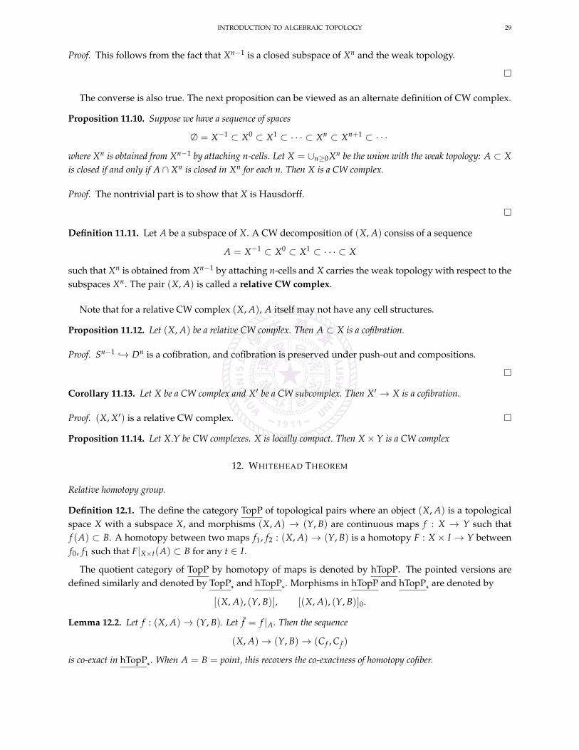
Lemma 12.5. f : (Dn, Sn−1) → (X, A) is zero in πn(X, A) if and only if f is homotopic rel Sn−1 to a map whoseimage lies in A.
This lemma can be summarized by the following diagram
Sn−1 _
// A _
Dn ''
f77
g==
X
Here g maps Dn to A and g ' f rel Sn−1.
Theorem 12.6. Let B ⊂ A ⊂ X in Top*. Then there is a long exact sequence
· · · → πn(A, B) i∗→ πn(X, B)j∗→ πn(X, A)
∂→ πn−1(A, B) · · · → π0(X)
Here the boundary map ∂ sends f ∈ [(Dn, Sn−1), (X, A)]0 to its restriction to Sn−1 = Dn−1/Sn−2 viewed as
∂ f : (Dn−1, Sn−2)→ (A, B)
where ∂ f sends the whole Sn−2 to the base point in B.
Proof. We prove the case for A = B = base point x0 ∈ X. Consider
f : (S0, 0)→ (S0, S0).
Let f = f |0 : 0 → S0. It is easy to see that
(C f , C f ) ' (D1, S0).
Since Σn(S0) = Sn, Σ(Dn, Sn−1) = (Dn+1, Sn), the co-exact Puppe sequence
(S0, 0)→ (S0, S0)→ (D1, S0)→ (S1, 0)→ (S1, S1)→ (D2, S1)→ (S2, 0)→ · · ·
implies the exact sequence
· · · → πn(A)i∗→ πn(X)
j∗→ πn(X, A)∂→ πn−1(A) · · · → π0(X)
Definition 12.7. A pair (X, A) is called n-connected (n ≥ 0) if π0(A)→ π0(X) is surjective and πk(X, A; x0) =
0 for any 1 ≤ k ≤ n, x0 ∈ A.
INTRODUCTION TO ALGEBRAIC TOPOLOGY 31
From the long exact sequence
· · · → πn(A)i∗→ πn(X)
j∗→ πn(X, A)∂→ πn−1(A) · · · → π0(X)
we see that (X, A) is n-connected if and only if for any x0 ∈ Aπr(A, x0)→ πr(X, x0) is bijective for r < n
πn(A, x0)→ πn(X, x0) is surjective
Definition 12.8. A map f : X → Y is called an n-equivalence (n ≥ 0) if for any x0 ∈ X f∗ : πr(X, x0)→ πr(Y, f (x0)) is bijective for r < n
f∗ : πn(X, x0)→ πn(Y, f (x0)) is surjective
f is called weak homotopy equivalence or ∞-equivalence if f is n-equivalence for any n ≥ 0.
Example 12.9. For any n ≥ 0, the pair (Dn+1, Sn) is n-connected.
CW complex.
Lemma 12.10. Let X be obtained from A by attaching n-cells. Let (Y, B) be a pair such that πn(Y, B; b) = 0, ∀b ∈ Bif n ≥ 1 or π0(B) → π0(Y) surjective if n = 0. Then any map from (X, A) → (Y, B) is homotopic rel A to a mapfrom X to B.
Proof. Apply the universal property of push-out and the result for Sn−1 → Dn.
ä Sn−1 // _
A _
// B _
ä Dn //
66
X&&88
@@
Y
Theorem 12.11. Let (X, A) be a relative CW complex with relative dimension ≤ n. Let (Y, B) be n-connected(0 ≤ n ≤ ∞). Then any map from (X, A) to (Y, B) is homotopic relative to A to a map from X to B.
A _
// B _
X
&&88
??
Y
Proof. Apply the previous Lemma to
A ⊂ X0 ⊂ X1 ⊂ · · · ⊂ Xn = X
and observe that all embeddings are cofibrations.
Proposition 12.12. Let f : X → Y be a weak homotopy equivalence, P be a CW complex. Then
f∗ : [P, X]→ [P, Y]
is a bijection.
32 SI LI
Proof. We can assume f is an embedding and (Y, X) is ∞-connected. Otherwise replace Y by M f .
Surjectivity follows from the diagram
∅ _
// X _
P
&&88
??
Y
Injectivity follows from the diagram (observe P× I, P× ∂I are CW complexes)
P× ∂I _
// X _
P× I
''77
<<
Y
Theorem 12.13 (Whitehead Theorem). A map between CW complexes is a weak homotopy equivalence if and onlyif it is a homotopy equivalence.
Proof. Let f : X → Y be a weak homotopy equivalence between CW complexes. We have bijections
f∗ : [X, X]0 → [X, Y]0, f∗ : [Y, X]→ [Y, Y]0.
Let g ∈ [Y, X]0 such that f∗[g] = 1Y. Then g f ' 1Y. On the other hand,
f∗[ f g] = [ f g f ] ' [ f 1] = [ f ] = f∗[1X ]
we find [ f g] = 1X . Therefore f is a homotopy equivalence. The reverse direction is obvious.
13. CELLULAR AND CW APPROXIMATIONS
Cellular Approximation.
Definition 13.1. Let (X, Y) be CW complexes. A map f : X → Y is called cellular if f (Xn) ⊂ Yn for any n.We define the category CW whose objects are CW complexes and morphisms are cellular maps.
Definition 13.2. A cellular homotopy between two cellular maps X → Y of CW complexes is a homotopyX × I → Y that is itself a cellular map. Here I is naturally a CW complex. We define the quotient categoryhCW of CW whose morphisms are cellular homotopy class of cellular maps.
Lemma 13.3. Let X be obtained from A by attaching n-cells (n ≥ 1), then (X, A) is (n− 1)-connected.
Proof. Let r < n. Consider a diagram
Sr−1 _
// A _
Dr f
// X
Since Dr is compact, f (Dr) meets only finitely many attached n-cells on X, say e1, · · · , em. Let pi be thecenter of ei. Let e∗i = ei − pi. Y = X − p1, · · · , pm. We subdivide Dr into small disks Dr = ∪αDr
α
such that f (Drα) ⊂ Y or f (Dr
α) ⊂ e∗i . For each Drα such that f (Dr
α) ⊂ ei but not in Y, we use the fact that
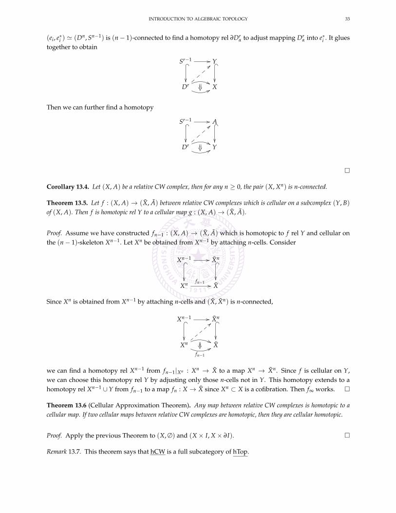
INTRODUCTION TO ALGEBRAIC TOPOLOGY 33
(ei, e∗i ) ' (Dn, Sn−1) is (n− 1)-connected to find a homotopy rel ∂Drα to adjust mapping Dr
α into e∗i . It gluestogether to obtain
Sr−1 _
// Y _
Dr ''
77
==
X
Then we can further find a homotopy
Sr−1 _
// A _
Dr &&
88
==
Y
Corollary 13.4. Let (X, A) be a relative CW complex, then for any n ≥ 0, the pair (X, Xn) is n-connected.
Theorem 13.5. Let f : (X, A) → (X, A) between relative CW complexes which is cellular on a subcomplex (Y, B)of (X, A). Then f is homotopic rel Y to a cellular map g : (X, A)→ (X, A).
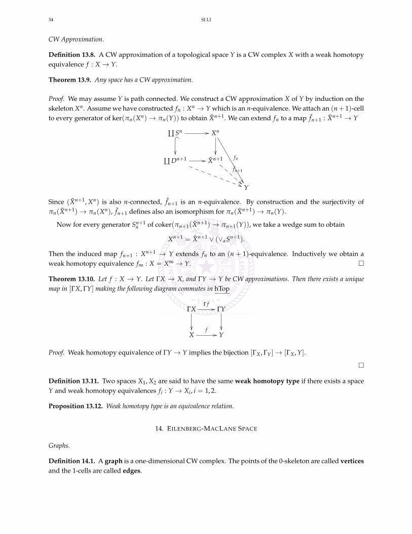
Proof. Assume we have constructed fn−1 : (X, A) → (X, A) which is homotopic to f rel Y and cellular onthe (n− 1)-skeleton Xn−1. Let Xn be obtained from Xn−1 by attaching n-cells. Consider
Xn−1 _
// Xn _
Xn fn−1 // X
Since Xn is obtained from Xn−1 by attaching n-cells and (X, Xn) is n-connected,
Xn−1 _
// Xn _
Xn ''
fn−1
77
<<
X
we can find a homotopy rel Xn−1 from fn−1|Xn : Xn → X to a map Xn → Xn. Since f is cellular on Y,we can choose this homotopy rel Y by adjusting only those n-cells not in Y. This homotopy extends to ahomotopy rel Xn−1 ∪Y from fn−1 to a map fn : X → X since Xn ⊂ X is a cofibration. Then f∞ works.
Theorem 13.6 (Cellular Approximation Theorem). Any map between relative CW complexes is homotopic to acellular map. If two cellular maps between relative CW complexes are homotopic, then they are cellular homotopic.
Proof. Apply the previous Theorem to (X, ∅) and (X× I, X× ∂I).
Remark 13.7. This theorem says that hCW is a full subcategory of hTop.
34 SI LI
CW Approximation.
Definition 13.8. A CW approximation of a topological space Y is a CW complex X with a weak homotopyequivalence f : X → Y.
Theorem 13.9. Any space has a CW approximation.
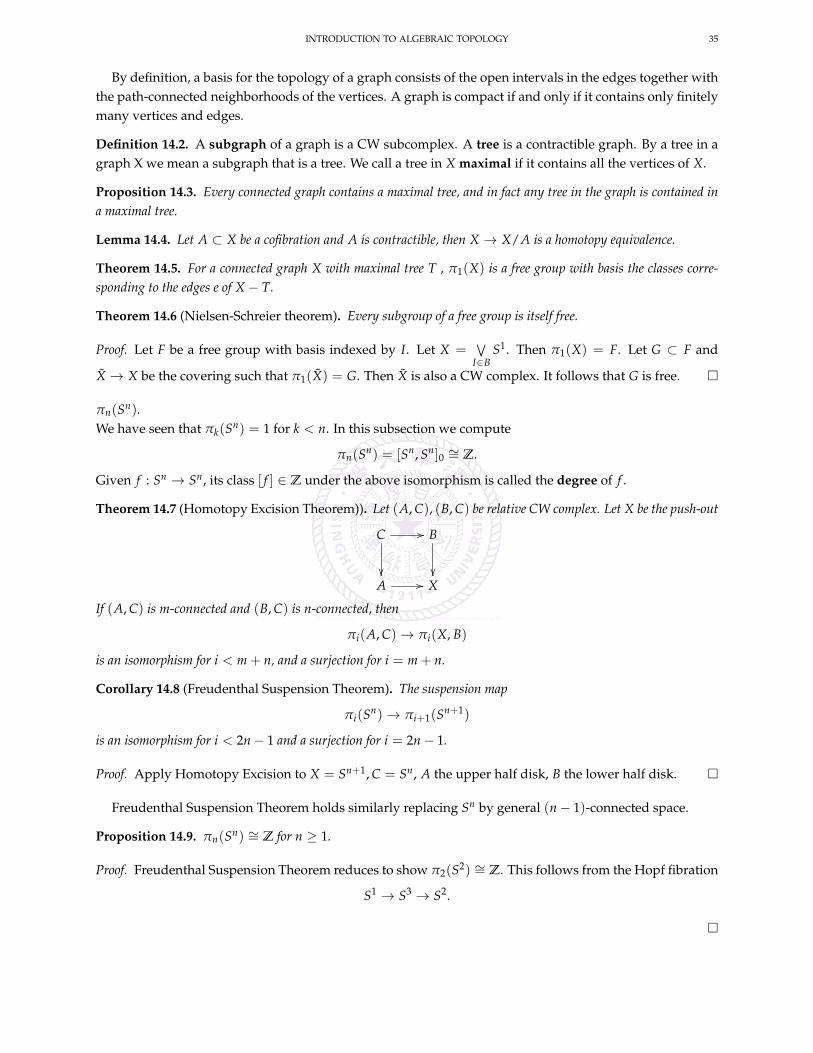
Proof. We may assume Y is path connected. We construct a CW approximation X of Y by induction on theskeleton Xn. Assume we have constructed fn : Xn → Y which is an n-equivalence. We attach an (n+ 1)-cellto every generator of ker(πn(Xn)→ πn(Y)) to obtain Xn+1. We can extend fn to a map fn+1 : Xn+1 → Y
ä Sn _
// Xn
fn
ä Dn+1 //
))
Xn+1
fn+1
!!Y
Since (Xn+1, Xn) is also n-connected, fn+1 is an n-equivalence. By construction and the surjectivity ofπn(Xn+1)→ πn(Xn), fn+1 defines also an isomorphism for πn(Xn+1)→ πn(Y).
Now for every generator Sn+1α of coker(πn+1(Xn+1)→ πn+1(Y)), we take a wedge sum to obtain
Xn+1 = Xn+1 ∨ (∨αSn+1).
Then the induced map fn+1 : Xn+1 → Y extends fn to an (n + 1)-equivalence. Inductively we obtain aweak homotopy equivalence f∞ : X = X∞ → Y.
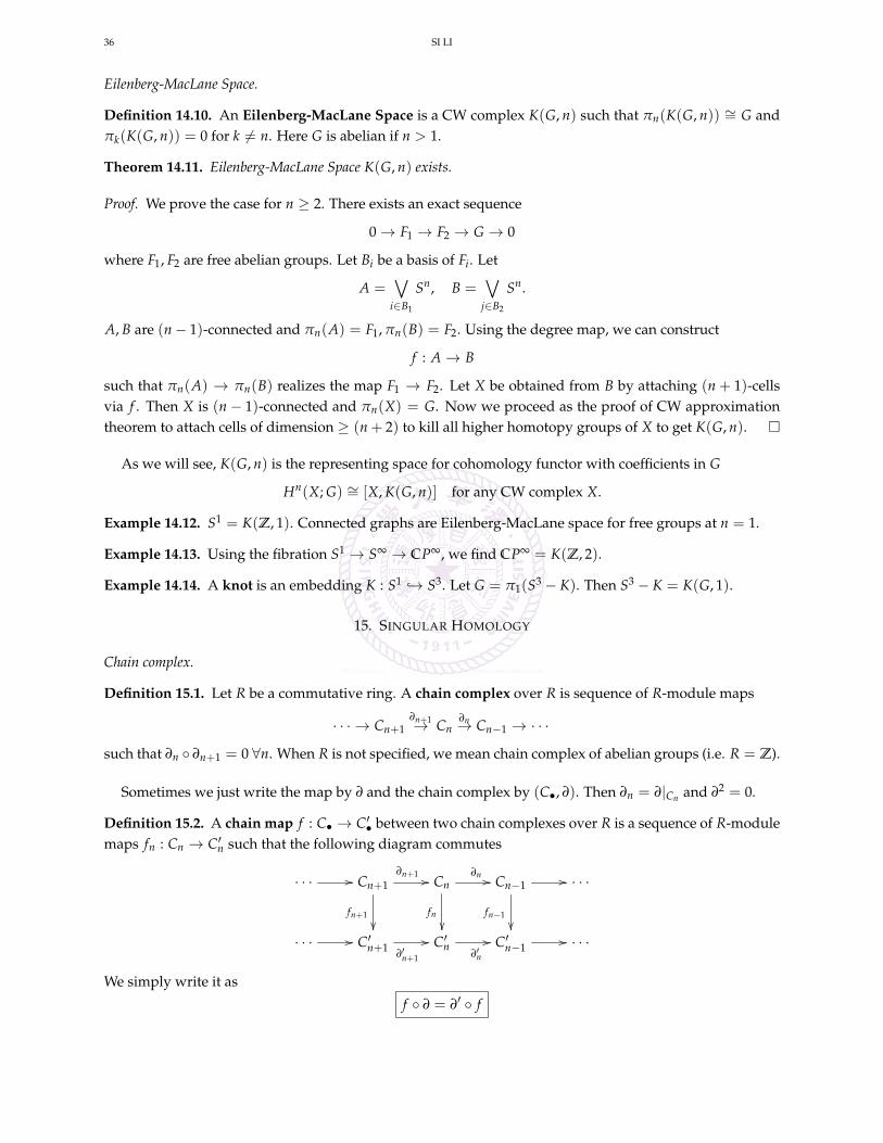
Theorem 13.10. Let f : X → Y. Let ΓX → X, and ΓY → Y be CW approximations. Then there exists a uniquemap in [ΓX, ΓY] making the following diagram commutes in hTop
ΓX
Γ f// ΓY
X
f// Y
Proof. Weak homotopy equivalence of ΓY → Y implies the bijection [ΓX , ΓY]→ [ΓX , Y].
Definition 13.11. Two spaces X1, X2 are said to have the same weak homotopy type if there exists a spaceY and weak homotopy equivalences fi : Y → Xi, i = 1, 2.
Proposition 13.12. Weak homotopy type is an equivalence relation.
14. EILENBERG-MACLANE SPACE
Graphs.
Definition 14.1. A graph is a one-dimensional CW complex. The points of the 0-skeleton are called verticesand the 1-cells are called edges.
INTRODUCTION TO ALGEBRAIC TOPOLOGY 35
By definition, a basis for the topology of a graph consists of the open intervals in the edges together withthe path-connected neighborhoods of the vertices. A graph is compact if and only if it contains only finitelymany vertices and edges.
Definition 14.2. A subgraph of a graph is a CW subcomplex. A tree is a contractible graph. By a tree in agraph X we mean a subgraph that is a tree. We call a tree in X maximal if it contains all the vertices of X.
Proposition 14.3. Every connected graph contains a maximal tree, and in fact any tree in the graph is contained ina maximal tree.
Lemma 14.4. Let A ⊂ X be a cofibration and A is contractible, then X → X/A is a homotopy equivalence.
Theorem 14.5. For a connected graph X with maximal tree T , π1(X) is a free group with basis the classes corre-sponding to the edges e of X− T.
Theorem 14.6 (Nielsen-Schreier theorem). Every subgroup of a free group is itself free.
Proof. Let F be a free group with basis indexed by I. Let X =∨
I∈BS1. Then π1(X) = F. Let G ⊂ F and
X → X be the covering such that π1(X) = G. Then X is also a CW complex. It follows that G is free.
πn(Sn).We have seen that πk(Sn) = 1 for k < n. In this subsection we compute
πn(Sn) = [Sn, Sn]0 ∼= Z.
Given f : Sn → Sn, its class [ f ] ∈ Z under the above isomorphism is called the degree of f .
Theorem 14.7 (Homotopy Excision Theorem)). Let (A, C), (B, C) be relative CW complex. Let X be the push-out
C //
B
A // X
If (A, C) is m-connected and (B, C) is n-connected, then
πi(A, C)→ πi(X, B)
is an isomorphism for i < m + n, and a surjection for i = m + n.
Corollary 14.8 (Freudenthal Suspension Theorem). The suspension map
πi(Sn)→ πi+1(Sn+1)
is an isomorphism for i < 2n− 1 and a surjection for i = 2n− 1.
Proof. Apply Homotopy Excision to X = Sn+1, C = Sn, A the upper half disk, B the lower half disk.
Freudenthal Suspension Theorem holds similarly replacing Sn by general (n− 1)-connected space.
Proposition 14.9. πn(Sn) ∼= Z for n ≥ 1.
Proof. Freudenthal Suspension Theorem reduces to show π2(S2) ∼= Z. This follows from the Hopf fibration
S1 → S3 → S2.
36 SI LI
Eilenberg-MacLane Space.
Definition 14.10. An Eilenberg-MacLane Space is a CW complex K(G, n) such that πn(K(G, n)) ∼= G andπk(K(G, n)) = 0 for k 6= n. Here G is abelian if n > 1.
Theorem 14.11. Eilenberg-MacLane Space K(G, n) exists.
Proof. We prove the case for n ≥ 2. There exists an exact sequence
0→ F1 → F2 → G → 0
where F1, F2 are free abelian groups. Let Bi be a basis of Fi. Let
A =∨
i∈B1
Sn, B =∨
j∈B2
Sn.
A, B are (n− 1)-connected and πn(A) = F1, πn(B) = F2. Using the degree map, we can construct
f : A→ B
such that πn(A) → πn(B) realizes the map F1 → F2. Let X be obtained from B by attaching (n + 1)-cellsvia f . Then X is (n− 1)-connected and πn(X) = G. Now we proceed as the proof of CW approximationtheorem to attach cells of dimension ≥ (n + 2) to kill all higher homotopy groups of X to get K(G, n).
As we will see, K(G, n) is the representing space for cohomology functor with coefficients in G
Hn(X; G) ∼= [X, K(G, n)] for any CW complex X.
Example 14.12. S1 = K(Z, 1). Connected graphs are Eilenberg-MacLane space for free groups at n = 1.
Example 14.13. Using the fibration S1 → S∞ → CP∞, we find CP∞ = K(Z, 2).
Example 14.14. A knot is an embedding K : S1 → S3. Let G = π1(S3 − K). Then S3 − K = K(G, 1).
15. SINGULAR HOMOLOGY
Chain complex.
Definition 15.1. Let R be a commutative ring. A chain complex over R is sequence of R-module maps
· · · → Cn+1∂n+1→ Cn
∂n→ Cn−1 → · · ·
such that ∂n ∂n+1 = 0 ∀n. When R is not specified, we mean chain complex of abelian groups (i.e. R = Z).
Sometimes we just write the map by ∂ and the chain complex by (C•, ∂). Then ∂n = ∂|Cn and ∂2 = 0.
Definition 15.2. A chain map f : C• → C′• between two chain complexes over R is a sequence of R-modulemaps fn : Cn → C′n such that the following diagram commutes
· · · // Cn+1
fn+1
∂n+1 // Cn
fn
∂n // Cn−1
fn−1
// · · ·
· · · // C′n+1∂′n+1
// C′n∂′n
// C′n−1// · · ·
We simply write it as
f ∂ = ∂′ f
INTRODUCTION TO ALGEBRAIC TOPOLOGY 37
Chain complexes over R together with chain maps form the category Ch•(R) of chain complexes over R,or simply Ch• when R = Z.
Definition 15.3. Given a chain complex (C•, ∂), its n-cycles Zn and n-boundaries Bn are
Zn = Ker(∂ : Cn → Cn−1), Bn = Im(∂ : Cn+1 → Cn).
∂2 = 0 implies Bn ⊂ Zn. We define the n-th homology group by
Hn(C•, ∂) :=Zn
Bn=
ker(∂n)
im(∂n+1).
A chain complex C• is called acyclic or exact if Hn(C•) = 0, ∀n.
Proposition 15.4. n-th homology group defines a functor
Hn : Ch• → Ab
Definition 15.5. A chain homotopy fs' g between two chain maps f , g : C• → C′• is a sequence of
homomorphisms sn : Cn → C′n+1 such that fn − gn = sn−1 ∂n + ∂′n+1 sn, or simply
f − g = s ∂ + ∂′ s .
Two complexes C•, C′• are called chain homotopy equivalent if there exists chain maps f : C• → C′• andh : C′• → C• such that f g ' 1 and g f ' 1.
Proposition 15.6. Chain homotopy defines an equivalence relation on chain maps and compatible with compositions.
In other word, chain homotopy defines an equivalence relation on Ch•. We define the quotient category
hCh• = Ch• / ' .
Chain homotopy equivalence becomes an equivalence in hCh•.
Proposition 15.7. Let f , g be chain homotopic chain maps. Then they induce identical map on homology groups
Hn( f ) = Hn(g) : Hn(C•)→ Hn(C′•).
In other words, the functor Hn factor through
Hn : Ch• → hCh• → Ab .
Singular homology.
Definition 15.8. We define the standard n-simplex
∆n = (t0, · · · , tn) ∈ Rn+1|n
∑i=0
ti = 1, ti ≥ 0
We let v0, · · · , vn denote its vertices. Here vi = (0, · · · , 0, 1, 0, · · · , 0) where 1 sits at the i-th position.
Definition 15.9. Let X be a topological space. A singular n-simplex in X is a continuous map σ : ∆n → X.For each n ≥ 0, we define Sn(X) as the free abelian group with basis all singular n-simplexes in X
Sn(X) =⊕
σ∈Hom(∆n ,X)
Zσ.
The elements of Sn(X) are called singular n-chains in X.
38 SI LI
A singular n-chain is given by a finite formal sum
γ = ∑σ∈Hom(∆n ,X)
mσσ, mσ ∈ Z and only finitely many mσ’s are nonzero.
The abelian group structure is: −γ := ∑σ(−mσ)σ and
(∑σ
mσσ) + (∑σ
m′σσ) = ∑σ
(mσ + m′σ)σ.
Definition 15.10. Given a n-simplex σ : ∆n → X and 0 ≤ i ≤ n, we define
∂(i)σ : ∆n−1 → X
to be the (n− 1)-simplex by restricting σ to the i-th face of ∆n whose vertices are given by v0, v1, · · · , vi, · · · , vn.We define the boundary map
∂ : Sn(X)→ Sn−1(X)
by the abelian group homomorphism generated by
∂σ :=n
∑i=0
(−1)i∂(i)σ .
Proposition 15.11. (S•(X), ∂) defines a chain complex, i.e., ∂2 = ∂ ∂ = 0.
Definition 15.12. For each n ≥ 0, we define n-th singular homology group of X by
Hn(X) := Hn(S•(X), ∂) .
Let f : X → Y be a continuous map, it defines a chain map
S•( f ) : S•(X)→ S•(Y).
This defines the functor of singular chain complex
S• : Top→ Ch• .
Singular homology group can be viewed as the composition of functors
Top→ Ch•Hn→ Ab .
Proposition 15.13. Let f , g : X → Y be homotopic maps. Then S•( f ), S•(g) : S•(X) → S•(Y) are chainhomotopic. In particular, they induce identical map Hn( f ) = Hn(g) : Hn(X)→ Hn(Y).
Proof. We only need to prove that for i0, i1 : X → X× I, the induced map
S•(i0), S•(i1) : S•(X)→ S•(X× I)
are chain homotopic. Then their composition with the homotopy X× I → Y gives the proposition.
Let us define a homotopys : Sn(X)→ Sn+1(X× I).
For σ : ∆n → X, we define (topologically)
s(σ) : ∆n × I σ×1→ X× I
Here we treat ∆n × I as a collection of (n + 1)-simplexes as follows: let v0, · · · , vn denote the vertices of∆n, then the vertices of ∆n × I contain two copies v0, · · · , vn and w0, · · · , wn. Then
∆n × I =n
∑i=0
(−1)n[v0, v1, · · · vi, wi, wi+1, · · · , wn]
INTRODUCTION TO ALGEBRAIC TOPOLOGY 39
cuts ∆n × I into (n + 1)-simplexes. Its sum defines s(σ) ∈ Sn+1(X× I). The intuitive formula holds
∂(∆n × I) = ∆× ∂I − (∂∆n)× I
as an equation for singular chains, leading to
S•(i1)− S•(i0) = ∂ s + s ∂.
Theorem 15.14. Singular homologies are homotopy invariants. They factor through
Hn : hTop→ hCh• → Ab .
16. EXACT HOMOLOGY SEQUENCE
Exact homology sequence.
Definition 16.1. Chain maps 0→ C′•i→ C•
p→ C′′• → 0 is called an short exact sequence if for each n
0→ C′ni→ Cn
p→ C′′n → 0
is an exact sequence of abelian groups.
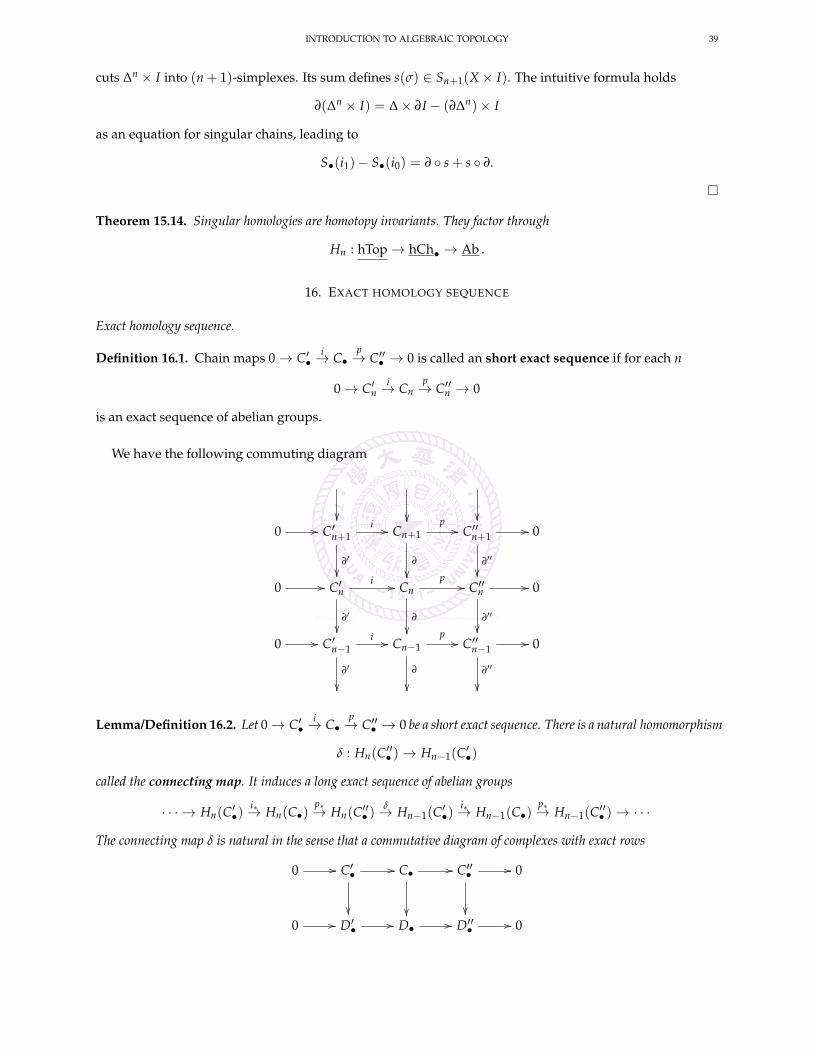
We have the following commuting diagram
0 // C′n+1
i //
∂′
Cn+1p//
∂
C′′n+1
∂′′
// 0
0 // C′ni //
∂′
Cnp//
∂
C′′n
∂′′
// 0
0 // C′n−1i //
∂′
Cn−1p//
∂
C′′n−1
∂′′
// 0
Lemma/Definition 16.2. Let 0→ C′•i→ C•
p→ C′′• → 0 be a short exact sequence. There is a natural homomorphism
δ : Hn(C′′• )→ Hn−1(C′•)
called the connecting map. It induces a long exact sequence of abelian groups
· · · → Hn(C′•)i∗→ Hn(C•)
p∗→ Hn(C′′• )δ→ Hn−1(C′•)
i∗→ Hn−1(C•)p∗→ Hn−1(C′′• )→ · · ·
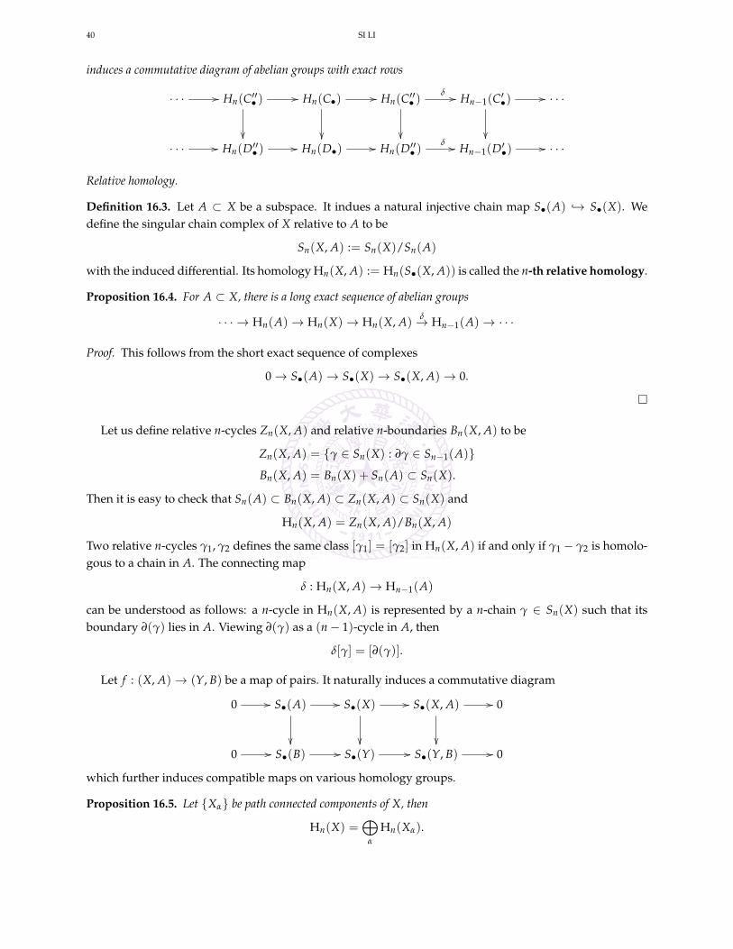
The connecting map δ is natural in the sense that a commutative diagram of complexes with exact rows
0 // C′• //
C• //
C′′• //
0
0 // D′• // D• // D′′• // 0
40 SI LI
induces a commutative diagram of abelian groups with exact rows
· · · // Hn(C′′• ) //
Hn(C•) //
Hn(C′′• )
δ // Hn−1(C′•) //
· · ·
· · · // Hn(D′′• ) // Hn(D•) // Hn(D′′• )δ // Hn−1(D′•) // · · ·
Relative homology.
Definition 16.3. Let A ⊂ X be a subspace. It indues a natural injective chain map S•(A) → S•(X). Wedefine the singular chain complex of X relative to A to be
Sn(X, A) := Sn(X)/Sn(A)
with the induced differential. Its homology Hn(X, A) := Hn(S•(X, A)) is called the n-th relative homology.
Proposition 16.4. For A ⊂ X, there is a long exact sequence of abelian groups
· · · → Hn(A)→ Hn(X)→ Hn(X, A)δ→ Hn−1(A)→ · · ·
Proof. This follows from the short exact sequence of complexes
0→ S•(A)→ S•(X)→ S•(X, A)→ 0.
Let us define relative n-cycles Zn(X, A) and relative n-boundaries Bn(X, A) to be
Zn(X, A) = γ ∈ Sn(X) : ∂γ ∈ Sn−1(A)
Bn(X, A) = Bn(X) + Sn(A) ⊂ Sn(X).
Then it is easy to check that Sn(A) ⊂ Bn(X, A) ⊂ Zn(X, A) ⊂ Sn(X) and
Hn(X, A) = Zn(X, A)/Bn(X, A)
Two relative n-cycles γ1, γ2 defines the same class [γ1] = [γ2] in Hn(X, A) if and only if γ1 − γ2 is homolo-gous to a chain in A. The connecting map
δ : Hn(X, A)→ Hn−1(A)
can be understood as follows: a n-cycle in Hn(X, A) is represented by a n-chain γ ∈ Sn(X) such that itsboundary ∂(γ) lies in A. Viewing ∂(γ) as a (n− 1)-cycle in A, then
δ[γ] = [∂(γ)].
Let f : (X, A)→ (Y, B) be a map of pairs. It naturally induces a commutative diagram
0 // S•(A) //
S•(X) //
S•(X, A) //
0
0 // S•(B) // S•(Y) // S•(Y, B) // 0
which further induces compatible maps on various homology groups.
Proposition 16.5. Let Xα be path connected components of X, then
Hn(X) =⊕
α
Hn(Xα).
INTRODUCTION TO ALGEBRAIC TOPOLOGY 41
Proposition 16.6. Let X be path connected. Then H0(X) ∼= Z.
In general, we have a surjective map
ε : H0(X)→ Z, ∑p∈X
mp p→∑p
mp.
Definition 16.7. We define the reduced homology group by
Hn(X) =
Hn(X) n > 0
ker(H0(X)→ Z) n = 0
The long exact sequence still holds for the reduced case
· · · → Hn(A)→ Hn(X)→ Hn(X, A)δ→ Hn−1(A)→ · · ·
Example 16.8. If X is contractible, then Hn(X) = 0 for all n.
Example 16.9. Let x0 ∈ X be a point. Using the long exact sequence for A = x0 ⊂ X, we find
Hn(X, x0) = Hn(X).
17. EXCISION
The fundamental property of homology which makes it computable is excision.
Barycentric Subdivision.
Definition 17.1. Let ∆n be the standard n-simplex with vertices v0, · · · , vn. We define its barycenter to be
c(∆n) =1
n + 1
n
∑i=0
vi ∈ ∆n.
Definition 17.2. We define the barycentric subdivision B∆n of a n-simplex ∆n as follows:
(1) B∆0 = ∆0.(2) Let F0, · · · , Fn be the n-simplexes of faces of ∆n+1. c be the barycenter of ∆n+1. Then B∆n+1 consists
of (n + 1)-simplexes with ordered vertices [c, w0, · · · , wn] where [w0, · · · , wn] is a n-simplexes inBF0, · · · , BFn.
Equivalently, a simplex in B∆n is indexed by a sequence S0 ⊂ S1 · · · ⊂ Sn = ∆n where Si is a face ofSi+1. Then its vertices are [c(Sn), c(Sn−1), · · · , c(S0)]. It is seen that ∆n is the union of simplexes in B∆n.
Definition 17.3. We define the n-chain of barycentric subdivision Bn by
Bn = ∑α
±σα ∈ Sn(∆n)
where the summation is over all sequence α = S0 ⊂ S1 · · · ⊂ Sn = ∆n. σα is the simplex with orderedvertices [c(Sn), c(Sn−1), · · · , c(S0)], viewed as a singular n-chain in ∆n. The sign ± is about orientation: ifthe orientation of [c(Sn), c(Sn−1), · · · , c(S0)] coincides with that of ∆n, we take +; otherwise we take −.

42 SI LI
Definition 17.4. We define the composition map denoted by
Sk(∆m)× Sn(∆k)→ Sn(∆m), σ× η → σ η.
This is defined on generators via the composition ∆n → ∆k → ∆m and extended linearly on singular chains.
Similarly, there is a natural map denoted by
Sn(∆m) : Sm(X)→ Sn(X), η : σ→ η∗(σ) = σ η
where η∗(σ) = σ η is the composition of σ with η.
Example 17.5. Let ∂n ∈ Sn−1(∆n) be the faces. Then ∂n ∂n−1 = 0 and
∂n = ∂∗n : Sn(X)→ Sn−1(x)
defines the boundary map in singular chains.
Lemma 17.6.Bn ∂n = ∂n Bn−1
Proof. The choice of ordering and orientation guarantees that
∂Bn = B(∂∆n)
where B(∂∆n) is the barycentric subdivision of faces ∂∆n of ∆n, viewed as a (n− 1)-chain in ∆n.
Definition 17.7. We define the barycentric subdivision on singular chain complex by
B∗ : S•(X)→ S•(X)
where B∗ = B∗n on Sn(X).
Lemma 17.8. B : S•(X)→ S•(X) is a chain map. Moreover, it is chain homotopic to the identity map.
Proof. The previous lemma implies
∂n B∗n = ∂∗n B∗n = (Bn ∂n)∗ = (∂n Bn−1)
∗ = B∗n−1 ∂n.
This show that B∗ is a chain map.
To show the chain homotopy, it is enough to construct Tn+1 ∈ Sn+1(∆n) such that
Bn − 1∆n = Tn+1 ∂n+1 + ∂n Tn.
Here 1∆n : ∆n → ∆n is the identity map, viewed as a n-chain. Then T∗n+1 gives the required homotopy. Tis constructed inductively in n as follows. T1 = 0. Suppose we have constructed Tn. We need to find Tn+1
such that∂(Tn+1) = Bn − 1∆n − ∂n Tn.
Observe
∂(Bn − 1∆n − ∂n Tn
)=(Bn − 1∆n − ∂n Tn
) ∂n = ∂n
(Bn−1 − 1∆n−1 − Tn ∂n
)= ∂n ∂n−1 Tn−1 = 0.
Therefore Bn − 1∆n − ∂n Tn is a n-cycle. However Hn(∆n) = 0 for n ≥ 1. It follows that Tn+1 can beconstructed.
Corollary 17.9. The barycentric subdivision map B∗ : S•(X)→ S•(X) is a quasi-isomorphism.
INTRODUCTION TO ALGEBRAIC TOPOLOGY 43
Excision.
Theorem 17.10 (Excision). Let U ⊂ A ⊂ X be subspaces such that U ⊂ A (the interior of A). Then the inclusioni : (X−U, A−U) → (X, A) induces isomorphisms
i∗ : Hn(X−U, A−U) ∼= Hn(X, A), ∀n.
Proof. Let us call σ : ∆n → X small if
σ(∆n) ⊂ A or σ(∆n) ⊂ X−U.
Let S′•(X) ⊂ S•(X) denote the subcomplex generated by small simplexes, and S′•(X, A) defined by theexact sequence
0→ S•(A)→ S′(X)→ S′(X, A)→ 0.
It is easy to see that
S′•(X, A) ∼= S•(X−U, A−U).
There is a natural commutative diagram of chain maps
0 // S•(A) //
S′•(X) //
S′•(X, A) //
0
0 // S•(A) // S•(X) // S•(X, A) // 0
By the Five Lemma, it is enough to show that
S′•(X)→ S•(X)
is a quasi-isomorphism.
(1) Injectivity of H(S′•(X))→ H(S•(X)):
Let α be a cycle in S′•(X) and α = ∂β for β ∈ S•(X). Take k big enough that (B∗)k(β) ∈ S′(X). Then
(B∗)k(α) = ∂(B∗)k(β).
Hence (B∗)k(α) is zero in H(S′•(X)), so is α which is homologous to (B∗)k(α).
(2) Surjectivity of H(S′•(X))→ H(S•(X)):
Let α be a cycle in S•(X). Take k big enough that (B∗)k(α) ∈ S′•(X). Then (B∗)k(α) is a small cyclewhich is homologous to α.
Theorem 17.11. Let X1, X2 be subspaces of X and X = X1 ∪ X2 . Then
H•(X1, X1 ∩ X2)→ H•(X, X2)
is an isomorphism for all n.
Proof. Apply Excision to U = X− X1, A = X2.
Theorem 17.12 (Mayer-Vietoris). Let X1, X2 be subspaces of X and X = X1 ∪X2 . Then there is an exact sequence
· · · → Hn(X1 ∩ X2)(i1∗ ,i2∗)→ Hn(X1)⊕Hn(X2)
j1∗−j2∗→ Hn(X)δ→ Hn−1(X1 ∩ X2)→ · · ·
It is also true for the reduced homology.

44 SI LI
Proof. Let S•(X1) + S•(X2) ⊂ S•(X) be the subspace spanned by S•(X1) and S•(X2). We have a short exactsequence
0→ S•(X1 ∩ X2)(i1,i2)→ S•(X1)⊕ S•(X2)
j1−j2→ S•(X1) + S•(X2)→ 0.
Similar to the proof of Excision via barycentric subdivision, the embedding S•(X1) + S•(X2) ⊂ S•(X) is aquasi-isomorphism. Mayer-Vietoris sequence follows.
Theorem 17.13. Let A ⊂ X be a closed subspace. Assume A is a strong deformation retract of a neighborhood in X.Then the map (X, A)→ (X/A, A/A) induces an isomorphism
H•(X, A) ∼= H•(X/A).
Proof. Let U be an open neighborhood of A that deformation retracts to A. Then H•(A) ∼= H•(U), hence
H•(X, A) ∼= H•(X, U)
by Five Lemma. Since A is closed and U is open, we can apply Excision to find
H•(X, A) ∼= H•(X, U) ∼= H•(X− A, U − A).
The same consideration applied to (X/A, A/A) and U/A gives
H•(X/A, A/A) ∼= H•(X/A− A/A, U/A− A/A) = H•(X− A, U − A).
This Theorem in particular applies to cofibrations.
18. HOMOLOGY OF SPHERES
Theorem 18.1. The reduced homology of the sphere Sn is given by
Hk(Sn) =
Z k = n
0 k 6= n
Proof. Let Sn = Dn+ ∪ Dn
−, where Dn+ (Dn
−) is the upper (lower) hemi-sphere and we choose a bit biggerones to satisfy excision. Dn
+ ∩ Dn− = Sn−1 × I ' Sn−1. Apply Mayer-Vietoris sequence we find
Hk(Sn) = Hk−1(Sn−1).
The theorem follows.
Corollary 18.2. If m 6= n, then Rm and Rn are not homeomorphic.
Definition 18.3. A continous map f : Sn → Sn (n ≥ 0) has degree d, denoted by deg( f ) = d, if
f∗ : Hn(Sn) = Z→ Hn(Sn) = Z
is multiplication by d.
Lemma 18.4. Let f , g : Sn → Sn be continuous maps.
(1) deg( f g) = deg( f )deg(g).(2) If f ' g are homotopic, then deg( f ) = deg(g)(3) If f is a homotopy equivalence, then deg( f ) = ±1.
INTRODUCTION TO ALGEBRAIC TOPOLOGY 45
Proposition 18.5. Let r : Sn → Sn, (x0, · · · , xn)→ (−x0, x1, · · · , xn) be the reflection. Then
deg(r) = −1.
Proof. Prove by induction on n. This is true for n = 0. The induction follows from the commutative diagram
Hn(Sn)
r∗
δ // Hn−1(Sn−1)
r∗
Hn(Sn)δ // Hn−1(Sn−1)
Corollary 18.6. Let σ : Sn → Sn, (x0, · · · , xn)→ (−x0, · · · ,−xn) be the antipodal map. Then
deg(σ) = (−1)n+1.
Proof. σ is a composition of n + 1 reflections.
Theorem 18.7 (Hairy Ball Theorem). Sn has a nowhere vanishing tangent vector field if and only if n is odd.
Proof. If n is odd, we construct
v(x0, · · · , xn) = (−x1, x0,−x3, x2, · · · ).
Conversely, assume v is no-where vanishing vector field. Let
f : Sn → Sn, x → v(x)|v(x)| .
The map
F : Sn × I → Sn, F(x, t) = cos(πt)x + sin(πt) f (x)
defines a homotopy between the identity map 1 and the antipodal map σ. It follows that
deg(σ) = 1 =⇒ n = odd.
Theorem 18.8 (Brower’s Fixed Point Theorem). Any continuous map f : Dn → Dn has a fixed point.
Proof. Assume f has no fixed point. Define
r : Dn → Sn−1
where r(p) is the intersection of ∂Dn with the ray starting from f (p) pointing toward p. Then r defines aretract of Sn−1 → Dn. This implies H•(Dn) = H•(Sn−1)⊕H•(Dn, Sn−1), a contradiction.
We give a geometric interpretation of the degree of f : Sn → Sn. Let V ⊂ Sn be a small open ball suchthat f−1(V)→ V is a disjoint union of open balls
f−1(V) = U1 ∪ · · · ∪Ud.
46 SI LI
Let fi : Ui/∂Ui∼= Sn → V/∂V ∼= Sn. We have the commutative diagram
Hn(Sn) //
f∗
Hn(Sn/Sn −∪iUi) ∼= ⊕i Hn(Sn)
⊕i( fi)∗
Hn(Sn) // Hn(Sn/Sn −V) ∼= Hn(Sn)
It is easy to see that first row is k→ (k, k, · · · , k) and the second row is k→ k. It follows that
deg( f ) =d
∑i=1
deg( fi).
Note that when f−1(V) → V is a covering map, then f : Ui → V is a homeomorphism. We havedeg( fi) = ±1 and deg( f ) is given by a counting with signs.
Example 18.9. Identify S2 = C∪ ∞. Consider the map f : S2 → S2, z→ zk. Then deg( f ) = k.
19. CELLULAR HOMOLOGY
Cellular homology.
Definition 19.1. Let (X, A) be a relative CW complex with skeletons: A = X−1 ⊂ X0 ⊂ · · · ⊂ Xn ⊂ · · · .We define the relative cellular chain complex (Ccell
• (X, A), ∂)
· · · → Ccelln (X, A)
∂→ Ccelln−1(X, A)
∂→ · · · → Ccell0 (X, A)→ 0
where Ccelln (X, A) := Hn(Xn, Xn−1) and the boundary map ∂ is defined by the commutative diagram
Hn(Xn, Xn−1)∂ //
δ
((
Hn−1(Xn−1, Xn−2)
Hn−1(Xn−1, A)
j55
Here δ is the connecting map of relative homology for A ⊂ Xn−1 ⊂ Xn and j is the natural map.
Assume Xn is obtained from Xn−1 by attaching n-cells indexed by Jn
äα∈Jn
Sn−1 f//
_
Xn−1 _
ä
α∈Jn
DnΦ f // Xn
Since Xn−1 → Xn is a cofibration,
Ccelln (X, A) ∼= Hn(Xn/Xn−1) ∼=
⊕Jn
Hn(Sn) ∼=⊕
Jn
Z
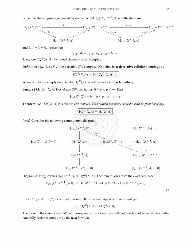
INTRODUCTION TO ALGEBRAIC TOPOLOGY 47
is the free abelian group generated by each attached Hn(Dn, Sn−1). Using the diagram
Hn(Xn, Xn−1)∂n //
δn
((
Hn−1(Xn−1, Xn−2)∂n−1 //
δn−1
))
Hn−2(Xn−2, Xn−3)
Hn−1(Xn−1, A)
jn55
Hn−1(Xn−2, A)
jn−155
and δn−1 jn = 0, we see that
∂n−1 ∂n = jn−1 δn−1 jn δn = 0.
Therefore (Ccell• (X, A), ∂) indeed defines a chain complex.
Definition 19.2. Let (X, A) be a relative CW complex. We define its n-th relative cellular homology by
Hcelln (X, A) := Hn(Ccell
• (X, A), ∂) .
When A = ∅, we simply denote it by Hcelln (X) called the n-th cellular homology.
Lemma 19.3. Let (X, A) be a relative CW complex. Let 0 ≤ q < p ≤ ∞. Then
Hn(Xp, Xq) = 0, n ≤ q or n > p.
Theorem 19.4. Let (X, A) be a relative CW complex. Then cellular homology coincides with singular homology
Hcelln (X, A) ∼= Hn(X, A) .
Proof. Consider the following commutative diagram
Hn+1(Xn+1, Xn)
∂n+1
))
Hn(Xn−2, A)(= 0)
Hn(Xn−1, A)(= 0) // Hn(Xn, A) //
Hn(Xn, Xn−1) //
∂n
))
Hn−1(Xn−1, A)
Hn(Xn+1, A)
Hn−1(Xn−1, Xn−2)
Hn(Xn+1, Xn)(= 0) Hn−1(Xn−2, A)(= 0)
Diagram chasing implies Hn(Xn+1, A) ∼= Hcelln (X, A). Theorem follows from the exact sequence
Hn+1(X, Xn+1)(= 0)→ Hn(Xn+1, A)→ Hn(X, A)→ Hn(X, Xn+1)(= 0)
Let f : (X, A)→ (Y, B) be a cellular map. It induces a map on cellular homology
f∗ : Hcell• (X, A)→ Hcell
• (Y, B).
Therefore in the category of CW complexes, we can work entirely with cellular homology which is combi-natorially easier to compute by the next formula.

48 SI LI
Cellular Boundary Formula.Let us now analyze cellular differential
∂n : Hn(Xn, Xn−1)→ Hn−1(Xn−1, Xn−2).
For each n-cell enα , we have the gluing map
fenα
: Sn−1 → Xn−1.
This defines a map
fenα
: Sn−1 → Xn−1/Xn−2 =∨
Jn−1
Sn−1
which induces a degree map
( fenα)∗ : Hn−1(Sn−1) ∼= Z→
⊕Jn−1
Hn−1(Sn−1) ∼=⊕Jn−1
Z.
Collecting all n-cells, this generates the degree map
dn :⊕
Jn
Z→⊕Jn−1
Z.
Theorem 19.5. Under the identification Ccelln (Xn, Xn−1) ∼=
⊕Jn
Z, cellular differential coincides with the degree map
∂n ∼= dn .
Example 19.6. CPn has a CW structure with a single 2m-cell for each m ≤ n. Since there is no odd dim cells,the degree map d = 0. We find
Hk(CPn) =
Z k = 0, 2, · · · , 2n
0 otherwise
Example 19.7. A closed oriented surface Σg of genus g has a CW structure with a 0-cell, 2g 1-cells, and a2-cell. It is easy to see that the degree map is zero. We find
Hk(Σg) =
Z k = 0
Z2g k = 1
Z k = 2
0 k > 2.
Example 19.8. RPn has a CW structure with a k-cell for each 0 ≤ k ≤ n. The degree map is dk = 1 + (−1)k.
Hk(RPn) =
Z k = 0
Z/2Z 0 < k < n, k odd
Z k = n = odd
0 k = n = even
0 k > n
INTRODUCTION TO ALGEBRAIC TOPOLOGY 49
Euler characteristic.
Definition 19.9. Let X be a finite CW complex of dimension n and denote by ci the number of i-cells of X.The Euler characteristic of X is defined as:
χ(X) := ∑i(−1)ici.
Recall that any finitely generaed abelian group G is decomposed into a free part and a torsion part
G ∼= Zr ⊕Z/m1Z⊕ · · · ⊕Z/mkZ.
The integer r := rk(G) is called the rank of G.
Theorem 19.10. Let X be a finite CW complex. Then
χ(X) = ∑i(−1)ibi(X)
where bi(X) := rk(Hi(X)) is called the i-th Betti number of X In particular, χ(X) is independent of the chosen CWstructure on X and only depend on the cellular homotopy class of X.
20. COHOMOLOGY AND UNIVERSAL COEFFICIENT THEOREM
Cohomology.
Definition 20.1. Let R be a commutative ring. A cochain complex over R is sequence of R-module maps
· · · → Cn−1 dn−1→ Cn dn→ Cn−1 → · · ·
such that dn dn−1 = 0 ∀n. When R is not specified, we mean cochain complex of abelian groups (i.e.R = Z).
Sometimes we just write the map by d and the cochain complex by (C•, d). Then dn = d|Cn and d2 = 0.
Definition 20.2. Given a cochain complex (C•, d), its n-cocycles Zn and n-coboundaries Bn are
Zn = Ker(d : Cn → Cn+1), Bn = Im(d : Cn−1 → Cn).
d2 = 0 implies Bn ⊂ Zn. We define the n-th cohomology group by
Hn(C•, d) :=Zn
Bn =ker(dn)
im(dn−1).
A cochain complex C• is called acyclic or exact if Hn(C•) = 0, ∀n.
We are interested in the following relation between cochain and chain complex.
Definition 20.3. Let (C•, ∂) be a chain complex over R, and G be a R-module. We define its dual cochaincomplex (C•, d) = HomR(C•, G) by
· · ·HomR(Cn−1, G)→ HomR(Cn, G)→ HomR(Cn+1, G)→ · · ·
Here given f ∈ HomR(Cn, G), we define dn f ∈ HomR(Cn+1, G) by
dn f (c) := f (∂n+1(c)), ∀c ∈ Cn+1.
50 SI LI
Definition 20.4. Let G be an abelian group and X be a topological space. For n ≥ 0, we define the group ofsingular n-cochains in X with coefficient in G to be
Sn(X; G) := Hom(Sn(X), G).
The dual cochain complex S•(X; G) = Hom(S•(X), G) is called the singular cochain complex with coeffi-cient in G. Its cohomology is called the singular cohomology with coefficient in G, denoted by
Hn(X; G) := Hn(S•(X; G)).
When G = Z, we simply write it as Hn(X).
Theorem 20.5. Hn(−; G) defines a contra-variant functor
Hn(−; G) : hTop→ Ab .
Example 20.6 (Dimension Axiom). Let X be a point. Then
Hn(X; G) =
G k = 0
0 k > 0
Lemma 20.7. Let G be a R-module. If 0→ A1 → A2 → A3 → 0 is an exact sequence of R-modules, then applyingHomR(−, G) gives an exact sequence
0→ HomR(A3, G)→ HomR(A2, G)→ HomR(A1, G).
If A3 is a free R-module (or more generally projective R-module), then the last morphism is also surjective.
Definition 20.8. Let G be an abelian group. Let A ⊂ X be a subspace. We define the relative singularcochain complex with coefficient in G by
S•(X, A; G) := Hom(S•(X)/S•(A), G).
Its cohomology is called the relative singular cohomology, denoted by H•(X, A; G).
Since S•(X)/S•(A) is a free abelian group, we have a short exact sequence of cochain complex
0→ S•(X, A; G)→ S•(X; G)→ S•(A; G)→ 0
which induces a long exact sequence of cohomology groups
0→ H0(X, A; G)→ H0(X; G)→ H0(A; G)→ H1(X, A; G)→ · · · .
Moreover, the connecting maps
δ : Hn(A, G)→ Hn+1(X, A; G)
is natural in the same sense as homology case.
Theorem 20.9 (Excision). Let U ⊂ A ⊂ X be subspaces such that U ⊂ A (the interior of A). Then the inclusioni : (X−U, A−U) → (X, A) induces isomorphisms
i∗ : Hn(X, A; G) ∼= Hn(X−U, A−U; G), ∀n.
INTRODUCTION TO ALGEBRAIC TOPOLOGY 51
Universal Coefficient Theorem for Cohomology.
Definition 20.10. Let M, N be two R-modules. Let P• → M be a free R-module resolution of M:
· · · Pn → Pn−1 → · · · P1 → P0 → M→ 0
is an exact sequence of R-modules and Pi’s are free. We define the Ext group
ExtkR(M, N) = Hk(Hom(P•, N))
and the Tor groupTorR
k (M, N) = Hk(P• ⊗R N).
Note thatExt0
R(M, N) = HomR(M, N), TorR0 (M, N) = M⊗R N.
Ext and Tor are called the derived functors of Hom and ⊗. It is a classical result in homological algebrathat Extk
R(M, N) and TorRk (M, N) don’t depend on the choice of resolution of M. They are functorial with
respect to both variables and TorRk is symmetric in two variables
TorRk (M, N) = TorR
k (N, M).
Moreover, for any short exact sequence of R-modules
0→ M1 → M2 → M3 → 0
there associate long exact sequences
0→ HomR(M3, N)→ HomR(M2, N)→ HomR(M1, N)
→ Ext1R(M3, N)→ Ext1
R(M2, N)→ Ext1R(M1, N)
→ Ext2R(M3, N))→ Ext2
R(M2, N)→ Ext2R(M1, N)→ · · ·
and
0→ HomR(N, M1)→ HomR(N, M2)→ HomR(N, M3)
→ Ext1R(N, M1)→ Ext1
R(N, M2)→ Ext1R(N, M3)
→ Ext2R(N, M1))→ Ext2
R(N, M2)→ Ext2R(N, M3)→ · · ·
and
· · · → TorR2 (M1, N)→ TorR
2 (M2, N)→ TorR3 (M3, N)
→ TorR1 (M1, N)→ TorR
1 (M2, N)→ TorR1 (M3, N)
→ M1 ⊗R N → M2 ⊗R N → M3 ⊗R N → 0
Now we focus on the case of abelian groups R = Z. For any abelian group M, let P0 be a free abeliangroup such that P0 → M is surjective. Let P1 be its kernel. Then P1 is also free and
0→ P1 → P0 → M→ 0
defines a free resolution of abelian groups. This implies that
Extk(M, N) = 0, Tork(M, N) = 0 for k ≥ 2.
In the case of abelian groups we will simply denote
Ext(M, N) := Ext1Z(M.N), Tor(M, N) := TorZ
1 (M, N) .
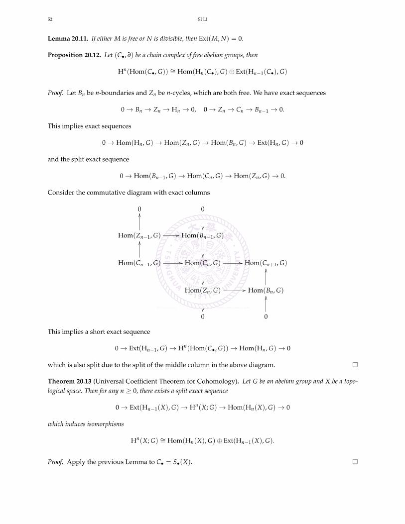
52 SI LI
Lemma 20.11. If either M is free or N is divisible, then Ext(M, N) = 0.
Proposition 20.12. Let (C•, ∂) be a chain complex of free abelian groups, then
Hn(Hom(C•, G)) ∼= Hom(Hn(C•), G)⊕ Ext(Hn−1(C•), G)
Proof. Let Bn be n-boundaries and Zn be n-cycles, which are both free. We have exact sequences
0→ Bn → Zn → Hn → 0, 0→ Zn → Cn → Bn−1 → 0.
This implies exact sequences
0→ Hom(Hn, G)→ Hom(Zn, G)→ Hom(Bn, G)→ Ext(Hn, G)→ 0
and the split exact sequence
0→ Hom(Bn−1, G)→ Hom(Cn, G)→ Hom(Zn, G)→ 0.
Consider the commutative diagram with exact columns
0 0
Hom(Zn−1, G) //
OO
Hom(Bn−1, G)
Hom(Cn−1, G) //
OO
Hom(Cn, G) //
Hom(Cn+1, G)
Hom(Zn, G) //
Hom(Bn, G)
OO
0 0
OO
This implies a short exact sequence
0→ Ext(Hn−1, G)→ Hn(Hom(C•, G))→ Hom(Hn, G)→ 0
which is also split due to the split of the middle column in the above diagram.
Theorem 20.13 (Universal Coefficient Theorem for Cohomology). Let G be an abelian group and X be a topo-logical space. Then for any n ≥ 0, there exists a split exact sequence
0→ Ext(Hn−1(X), G)→ Hn(X; G)→ Hom(Hn(X), G)→ 0
which induces isomorphisms
Hn(X; G) ∼= Hom(Hn(X), G)⊕ Ext(Hn−1(X), G).
Proof. Apply the previous Lemma to C• = S•(X).
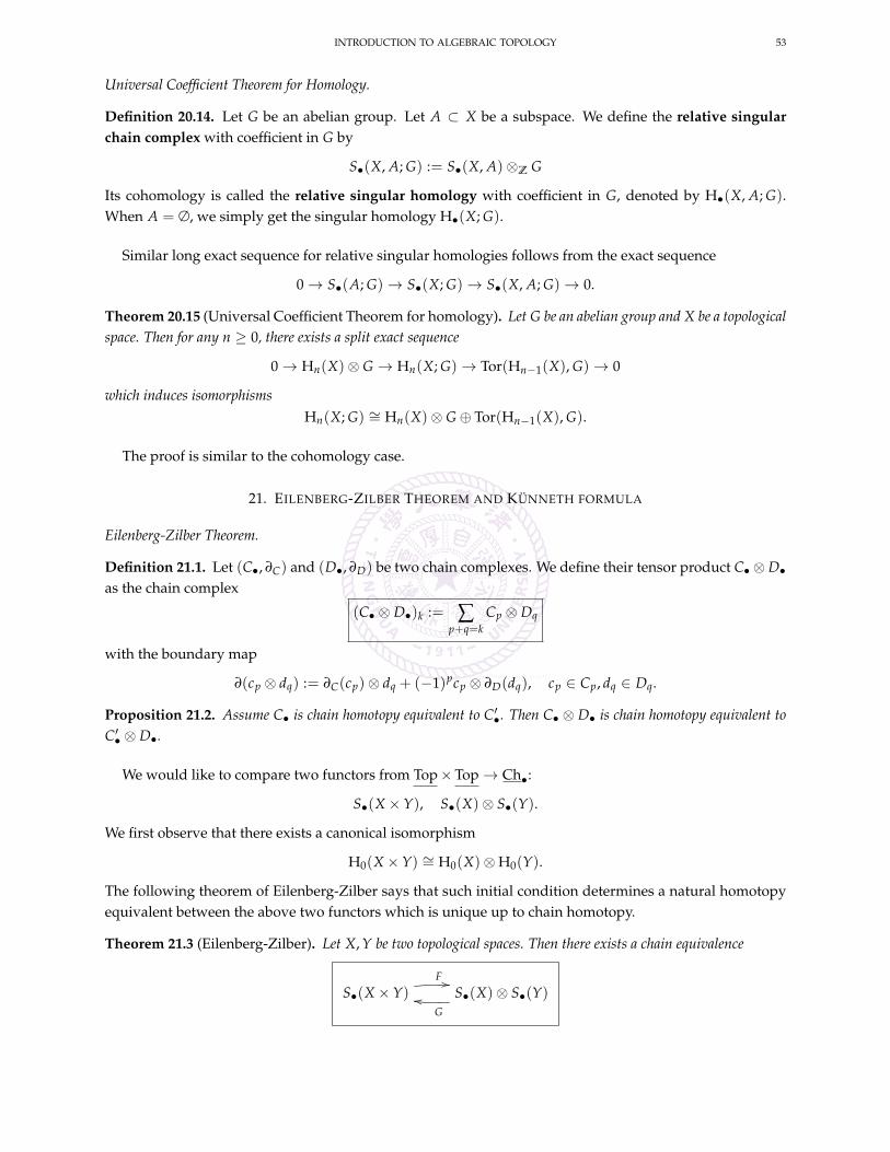
INTRODUCTION TO ALGEBRAIC TOPOLOGY 53
Universal Coefficient Theorem for Homology.
Definition 20.14. Let G be an abelian group. Let A ⊂ X be a subspace. We define the relative singularchain complex with coefficient in G by
S•(X, A; G) := S•(X, A)⊗Z G
Its cohomology is called the relative singular homology with coefficient in G, denoted by H•(X, A; G).When A = ∅, we simply get the singular homology H•(X; G).
Similar long exact sequence for relative singular homologies follows from the exact sequence
0→ S•(A; G)→ S•(X; G)→ S•(X, A; G)→ 0.
Theorem 20.15 (Universal Coefficient Theorem for homology). Let G be an abelian group and X be a topologicalspace. Then for any n ≥ 0, there exists a split exact sequence
0→ Hn(X)⊗ G → Hn(X; G)→ Tor(Hn−1(X), G)→ 0
which induces isomorphismsHn(X; G) ∼= Hn(X)⊗ G⊕ Tor(Hn−1(X), G).
The proof is similar to the cohomology case.
21. EILENBERG-ZILBER THEOREM AND KUNNETH FORMULA
Eilenberg-Zilber Theorem.
Definition 21.1. Let (C•, ∂C) and (D•, ∂D) be two chain complexes. We define their tensor product C• ⊗D•as the chain complex
(C• ⊗ D•)k := ∑p+q=k
Cp ⊗ Dq
with the boundary map
∂(cp ⊗ dq) := ∂C(cp)⊗ dq + (−1)pcp ⊗ ∂D(dq), cp ∈ Cp, dq ∈ Dq.
Proposition 21.2. Assume C• is chain homotopy equivalent to C′•. Then C• ⊗ D• is chain homotopy equivalent toC′• ⊗ D•.
We would like to compare two functors from Top×Top→ Ch•:
S•(X×Y), S•(X)⊗ S•(Y).
We first observe that there exists a canonical isomorphism
H0(X×Y) ∼= H0(X)⊗H0(Y).
The following theorem of Eilenberg-Zilber says that such initial condition determines a natural homotopyequivalent between the above two functors which is unique up to chain homotopy.
Theorem 21.3 (Eilenberg-Zilber). Let X, Y be two topological spaces. Then there exists a chain equivalence
S•(X×Y)F ..
S•(X)⊗ S•(Y)G
mm
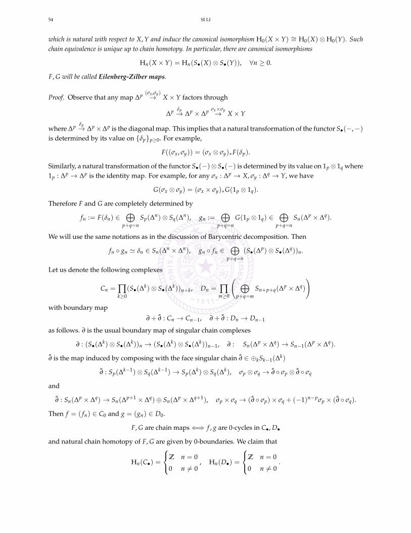
54 SI LI
which is natural with respect to X, Y and induce the canonical isomorphism H0(X × Y) ∼= H0(X)⊗H0(Y). Suchchain equivalence is unique up to chain homotopy. In particular, there are canonical isomorphisms
Hn(X×Y) = Hn(S•(X)⊗ S•(Y)), ∀n ≥ 0.
F, G will be called Eilenberg-Zilber maps.
Proof. Observe that any map ∆p (σx ,σy)→ X×Y factors through
∆p δp→ ∆p × ∆p σx×σy→ X×Y
where ∆p δp→ ∆p×∆p is the diagonal map. This implies that a natural transformation of the functor S•(−,−)is determined by its value on δpp≥0. For example,
F((σx, σy)) = (σx ⊗ σy)∗F(δp).
Similarly, a natural transformation of the functor S•(−)⊗ S•(−) is determined by its value on 1p⊗ 1q where1p : ∆p → ∆p is the identity map. For example, for any σx : ∆p → X, σy : ∆q → Y, we have
G(σx ⊗ σy) = (σx × σy)∗G(1p ⊗ 1q).
Therefore F and G are completely determined by
fn := F(δn) ∈⊕
p+q=nSp(∆n)⊗ Sq(∆n), gn :=
⊕p+q=n
G(1p ⊗ 1q) ∈⊕
p+q=nSn(∆p × ∆q).
We will use the same notations as in the discussion of Barycentric decomposition. Then
fn gn ' δn ∈ Sn(∆n × ∆n), gn fn ∈⊕
p+q=n(S•(∆p)⊗ S•(∆q))n.
Let us denote the following complexes
Cn = ∏k≥0
(S•(∆k)⊗ S•(∆k))n+k, Dn = ∏m≥0
( ⊕p+q=m
Sn+p+q(∆p × ∆q)
)with boundary map
∂ + ∂ : Cn → Cn−1, ∂ + ∂ : Dn → Dn−1
as follows. ∂ is the usual boundary map of singular chain complexes
∂ : (S•(∆k)⊗ S•(∆k))n → (S•(∆k)⊗ S•(∆k))n−1, ∂ : Sn(∆p × ∆q)→ Sn−1(∆p × ∆q).
∂ is the map induced by composing with the face singular chain ∂ ∈ ⊕kSk−1(∆k)
∂ : Sp(∆k−1)⊗ Sq(∆k−1)→ Sp(∆k)⊗ Sq(∆k), σp ⊗ σq → ∂ σp ⊗ ∂ σq
and
∂ : Sn(∆p × ∆q)→ Sn(∆p+1 × ∆q)⊕ Sn(∆p × ∆q+1), σp × σq → (∂ σp)× σq + (−1)n−pσp × (∂ σq).
Then f = ( fn) ∈ C0 and g = (gn) ∈ D0.
F, G are chain maps⇐⇒ f , g are 0-cycles in C•, D•
and natural chain homotopy of F, G are given by 0-boundaries. We claim that
Hn(C•) =
Z n = 0
0 n 6= 0, Hn(D•) =
Z n = 0
0 n 6= 0.
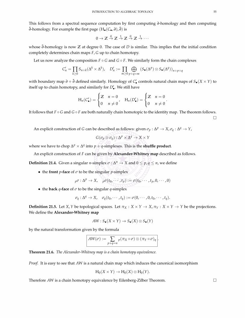
INTRODUCTION TO ALGEBRAIC TOPOLOGY 55
This follows from a spectral sequence computation by first computing ∂-homology and then computing∂-homology. For example the first page (H•(C•, ∂), ∂) is
0→ Z0→ Z
1→ Z0→ Z
1→ · · ·
whose ∂-homology is now Z at degree 0. The case of D is similar. This implies that the initial conditioncompletely determines chain maps F, G up to chain homotopy.
Let us now analyze the composition F G and G F. We similarly form the chain complexes
C′n = ∏k≥0
Sn+k(∆k × ∆k), D′n := ∏
m≥0
⊕p+q=m
(S•(∆p)⊗ S•(∆q))n+p+q
with boundary map ∂ + ∂ defined similarly. Homology of C′• controls natural chain maps of S•(X × Y) toitself up to chain homotopy, and similarly for D′•. We still have
Hn(C′•) =
Z n = 0
0 n 6= 0, Hn(D′•) =
Z n = 0
0 n 6= 0.
It follows that F G and G F are both naturally chain homotopic to the identity map. The theorem follows.
An explicit construction of G can be described as follows: given σp : ∆p → X, σq : ∆q → Y,
G(σp ⊗ σq) : ∆p × ∆q → X×Y
where we have to chop ∆p × ∆q into p + q-simplexes. This is the shuffle product.
An explicit construction of F can be given by Alexander-Whitney map described as follows.
Definition 21.4. Given a singular n-simplex σ : ∆n → X and 0 ≤ p, q ≤ n, we define
• the front p-face of σ to be the singular p-simplex
pσ : ∆p → X, pσ(t0, · · · , tp) := σ(t0, · · · , tp, 0, · · · , 0)
• the back q-face of σ to be the singular q-simplex
σq : ∆q → X, σq(t0, · · · , tq) := σ(0, · · · , 0, t0, · · · , tq).
Definition 21.5. Let X, Y be topological spaces. Let πX : X × Y → X, πY : X × Y → Y be the projections.We define the Alexander-Whitney map
AW : S•(X×Y)→ S•(X)⊗ S•(Y)
by the natural transformation given by the formula
AW(σ) := ∑p+q=n
p(πX σ)⊗ (πY σ)q .
Theorem 21.6. The Alexander-Whitney map is a chain homotopy equivalence.
Proof. It is easy to see that AW is a natural chain map which induces the canonical isomorphism
H0(X×Y)→ H0(X)⊗H0(Y).
Therefore AW is a chain homotopy equivalence by Eilenberg-Zilber Theorem.
56 SI LI
Kunneth formula.
Theorem 21.7 (Algebraic Kunneth formula). Let C• and D• be chain complex of free abelian groups. Then thereis a split exact sequence
0→ (H•(C)⊗H•(D))n → Hn(C• ⊗ D•)→ Tor(H•(C), H•(D))n−1 → 0.
Here Tor(H•(C), H•(D))k =⊕
p+q=kTor(Hp(C), Hq(D)).
Proof. Using the freeness of C• we can show that
H•(C• ⊗ D•) = H•(C• ⊗H•(D)).
Applying Universal Coefficient Theorem for Homology, we find
0→ Hp(C)⊗Hq(D)→ Hp+q(C•−q ⊗Hq(D))→ Tor(Hp−1(C), Hq(D))→ 0.
Summing over p, q gives the theorem.
Theorem 21.8 (Kunneth formula). For any topological spaces X, Y and n ≥ 0, there is a split exact sequence
0→⊕
p+q=nHp(X)⊗ Hq(X)→ Hn(X×Y)→
⊕p+q=n−1
Tor(Hp(X), Hq(Y))→ 0 .
Proof. This follows from Eilenberg-Zilber Theorem and algebraic Kunneth formula.
22. CUP AND CAP PRODUCT
Let R be a commutative ring with unit. We have natural cochain maps
S•(X; R)⊗R S•(Y; R)→ Hom(S•(X)⊗ S•(Y), R)→ S•(X×Y; R)
where the first map maps ϕp ∈ Sp(X; R), ηq ∈ Sq(X; R) to ϕp ⊗ ηq where
ϕp ⊗ ηq : σp ⊗ σq → ϕp(σp) · ηq(σq), σp ∈ Sp(X), σq ∈ Sq(X).
Here · is the product in R. This leads to a cochain map
S•(X; R)⊗R S•(Y; R)→ S•(X×Y; R)
which further inducesH•(X; R)⊗R H•(Y; R)→ H•(X×Y; R)
Cup product.
Definition 22.1. Let R be a commutative ring with unit. We define the cup product on cohomology groups
∪ : Hp(X; R)⊗R Hq(X; R)→ Hp+q(X; R)
by the composition
H•(X; R)⊗R H•(X; R)∪
))
// H•(X× X; R)
∆∗
H•(X; R)
Here ∆ : X → X× X is the diagonal map.
INTRODUCTION TO ALGEBRAIC TOPOLOGY 57
Alexander-Whitney map gives a specific product formula
(α ∪ β)(σ) = α(pσ) · β(σq) , α ∈ Sp(X; R), β ∈ Sq(X; R), σ : ∆p+q → X.
Theorem 22.2. H•(X; R) is a graded commutative ring with uint:
(1) Unit: let 1 ∈ H0(X; R) be represented by the cocyle which takes every singular 0-simplex to 1 ∈ R. Then
1∪ α = α ∪ 1 = α, ∀α ∈ H•(X; R).
(2) Associativity:(α ∪ β) ∪ γ = α ∪ (β ∪ γ).
(3) Graded commutativity:
α ∪ β = (−1)pqβ ∪ α, ∀α ∈ Hp(X; R), β ∈ Hq(X; R).
Proof. Unit of 1 is checked easily. Observe that the following two compositions of Eilenberg-Zilber mapsare chain homotopic (similar to Eilenberg-Zilber Theorem)
S•(X×Y× Z)→ S•(X×Y)⊗ S•(Z)→ S•(X)⊗ S•(Y)⊗ S•(Z)
S•(X×Y× Z)→ S•(X)⊗ S•(Y× Z)→ S•(X)⊗ S•(Y)⊗ S•(Z).
Associativity follows from the commutative diagram (R is hidden for simplicity)
H•(X)⊗H•(X)⊗H•(X) //
H•(X× X)⊗H•(X)
(∆×1)∗// H•(X)⊗H•(X)
H•(X)⊗H•(X× X) //
(1×∆)∗
H•(X× X× X)(∆×1)∗
//
(1×∆)∗
H•(X× X)
∆∗
H•(X)⊗H•(X) // H•(X× X)
∆∗ // H•(X)
Graded commutativity follows from the fact that the interchange map of tensor product of chain complexes
T : C• ⊗ D• → D• ⊗ C•
cp ⊗ dq → (−1)pqdq ⊗ cp
is a chain isomorphism. Therefore the two chain maps
S•(X×Y)→ S•(Y× X)→ S•(Y)⊗ S•(X)
S•(X×Y)→ S•(X)× S•(Y)T→ S•(Y)⊗ S•(X)
are chain homotopic, again by the uniqueness in Eilenberg-Zilber Theorem.
Set Y = X we find the following commutative diagram
H•(X)⊗H•(X) //
T
H•(X× X)
=
H•(X)⊗H•(X) // H•(X× X).
which gives graded commutativity.
Alternately, all the above can be checked explicitly using Alexander-Whitney map
58 SI LI
Theorem 22.3. Let f : X → Y be a continuous map. Then
f ∗ : H•(Y; R)→ H•(X; R)
is a morphism of graded commutative rings, i.e. f ∗(α ∪ β) = f ∗α ∪ f ∗β. In other words, H•(−) defines a functorfrom the category of topological spaces to the category of graded commutative rings.
Proof. The theorem follows from the commutative diagram
Xf
//
∆
Y
∆
X× Xf× f// Y×Y.
Theorem 22.4 (Kunneth formula). Assumem R is a PID, and Hi(X; R) are finitely generated R-module, then thereexists a split exact sequence of R-modules
0→⊕
p+q=nHp(X; R)⊗Hq(Y; R)→ Hn(X×Y; R)→
⊕p+q=n+1
TorR1 (H
p(X; R), Hq(Y; R)).
In particular, if H•(X; R) or H•(Y; R) are free R-modules, we have an isomorphism of graded commutative rings
H•(X×Y; R) ∼= H•(X; R)⊗R H•(Y; R).
Example 22.5. H•(Sn) = Z[η]/η2 where η ∈ Hn(Sn) is a generator.
Example 22.6. Let Tn = S1 × · · · × S1 be the n-torus. Then
H•(Tn) ∼= Z[η1, · · · , ηn], ηiη= − ηjηi
is the exterior algebra with n generators. Each ηi corresponds a generator of H1(S1).
Proposition 22.7. H•(CPn) = Z[x]/xn+1, where x ∈ H2(CPn) is a generator.
Proof. We prove by induction n. We know that
Hk(CPn) =
Z k = 2m ≤ 2n
0 otherwise
Let x be a generator of H2(CPn). We only need to show that xk is a generator of H2k(CPn) for each k ≤ n.Using cellular chain complex, we know that for k < n
H2k(CPn)→ H2k(CPk)
is an isomorphism. By induction, this implies that xk is a generator of H2k(CPn) for k < n. Poincare dualitytheorem (which will be proved in the next section) implies that
H2(CPn)⊗H2n−2(CPn)∪→ H2n(CPn)
is an isomorphism. This says that xn is a generator of H2n(CPn). This proves the proposition.
INTRODUCTION TO ALGEBRAIC TOPOLOGY 59
Cap product.
Definition 22.8. We define the evaluation map
〈−,−〉 : S•(X; R)×R S•(X; R)→ R
as follows: for α ∈ Sp(X; R), σ ∈ Sp(X), r ∈ R,
〈α, σ⊗ r〉 := α(σ) · r.
The evaluation map is compatible with boundary map and induces an evaluation map
〈−,−〉 : Hp(X; R)⊗R Hp(X; R)→ R.
This generalized to
S•(X; R)⊗R S•(X×Y; R)→ S•(X; R)⊗R S•(X; R)⊗R S•(Y; R)〈−,−〉⊗1→ S•(Y; R)
which induces
Hp(X; R)⊗R Hp+q(X×Y; R)→ Hq(Y; R).
Definition 22.9. We define the cap product
∩ : Hp(X; R)⊗Hp+q(X; R)→ Hq(X; R)
by the composition
Hp(X; R)⊗Hp+q(X; R)1⊗∆//
∩
**
Hp(X; R)⊗Hp+q(X× X; R)
Hq(X; R)
Theorem 22.10. The cap product gives H•(X; R) a structure of H•(X; R)-module.
Theorem 22.11. The cap product extends naturally to the relative case: for any pair A ⊂ X
∩ : Hp(X, A)⊗Hp+q(X, A)→ Hq(X)
∩ : Hp(X)⊗Hp+q(X, A)→ Hq(X, A)
Proof. Since S•(X, A) ⊂ S•(X), we have
∩ : S•(X, A)× S•(X)→ S•(X).
We model the cap product on chains via the Alexander-Whitney map. Then
∩ : S•(X, A)× S•(A)→ 0.
Therefore ∩ factors through
∩ : S•(X, A)× S•(X)
S•(A)→ S•(X).
Passing to homology (cohomology) we find the first cap product. The second one is proved similarly using
∩ : S•(X)× S•(X)
S•(A)→ S•(X)
S•(A).
60 SI LI
23. POINCARE DUALITY
Definition 23.1. A topological manifold of dimension n , or a topological n-manifold, is a Hausdorff spacein which each point has an open neighborhood homeomorphic to Rn.
In this section, a manifold always means a topological manifold. For any point x ∈ X, there exists anopen neighborhood U and a homeomorphism φ : U → Rn. (U, φ) is called a chart around x.
Orientation.
Definition 23.2. Let X be a n-manifold. x ∈ X be a point. A generator of
Hn(X, X− x) ∼= Hn(Rn, Rn − 0) ∼= Z
is called a local orientation of X at x.
For any x ∈ X, there are two choices of local orientation at x. We obtain a two-sheet cover
π : X → X, where X = (x, µx)|µx is a local orientation of X at x
Here π is the natural projection (x, µx) → x. X is topologized as follows. Let U be a small open ball in X.Then for any x ∈ U, we have an isomorphism
Hn(X, X−U) ∼= Hn(X, X− x)
which induces a set theoretical identification
π−1(U) ∼= U ×Z2.
Then we give a topology on X by requiring all such identifications being homeomorphisms. In particular,π : X → X is a Z2-covering map.
Definition 23.3. A (global) orientation of X is a section of π : X → X, i.e., a continuous map s : X → Xsuch that π s = 1X . If an orientation exists, we say X is orientable.
Theorem 23.4. Let X be a connected manifold. Then X is orientable if and only if X has two connected components.In particular, a connected orientable manifold has precisely two orientations.
Example 23.5. A simply connected manifold is orientable.
Example 23.6. Let X be connected non-orientable manifold. Then X is connected orientable.
Lemma 23.7. Let U ⊂ Rn be open. Then the natural map
Hn(Rn, U)→ ∏
x∈Rn−UHn(R
n, Rn − x)
is injective.
Proof. This is equivalent to the injectivity of
Hn−1(U)→ ∏x∈Rn−U
Hn−1(Rn − x).
Let α be a singular (n− 1)-chain representing a class [α]U in Hn−1(U). We can choose a big ball B containingU and finite small cubes D1, · · · , DN such that Di is not a subset of U but
Supp(α) ⊂ B− D1 ∪ · · · ∪ DN ⊂ U.
INTRODUCTION TO ALGEBRAIC TOPOLOGY 61
Then α represents a class in Hn−1(D1 ∪ · · · ∪ DN) ∼= Hn(B, B− D1 ∪ · · · ∪ DN) which maps to zero in eachHn(B, B−Di) ∼= Hn(B, B− xi) where xi ∈ Di −U. It follows via Mayer-Vietoris argument that α is the zeroclass in Hn−1(D1 ∪ · · · ∪ DN), hence zero in Hn−1(U).
Fundamental class.
Theorem 23.8. Let X be a connected n-manifold. For any abelian group G, we have the following vanishing statementHi(X; G) = 0 i > n
Hn(X; G) = 0 if X is noncompact.
Proof. We prove the case for G = Z. General G is similar. We assume X is connected.
Step 1: X = U ⊂ Rn is an open subset.
Let α ∈ Si(U) represent an element of [α] ∈ Hi(U). Let K ⊂ U be a compact subset such that Supp(α) ∈K. Equip Rn with a CW structure in terms of small enough cubes such that
K ⊂ L ⊂ U
where L is a finite CW subcomplex. We have a commutative diagram
Hi+1(Rn, L) //
Hi+1(Rn, U)
Hi(L) // Hi(U)
By construction, [α] ∈ Hi(U) lies in the image of Hi(L). But Hi+1(Rn, L) ∼= Hcell
i+1(Rn, L) = 0 for i ≥ n.
Step 2: X = U ∪V where U open is homeomorphic to Rn and V open satisfies the vanishing condition.
Consider the Mayer-Vietoris sequence
Hi(U)⊕ Hi(V)→ Hi(U ∪V)→ Hi−1(U ∩V)→ Hi−1(U)⊕ Hi−1(V)
For i > n, we find Hi(U ∪V) = 0 by Step 1. Assume that X = U ∪V is not compact. We need to prove
Hn−1(U ∩V)→ Hn−1(V)
is injective. The noncompactness and connectedness of X implies that
Hn(U ∪V)→ Hn(U ∪V, U ∪V − x)
is zero map for any x ∈ X. Consider the commutative diagram, where x ∈ U −U ∩V
Hn(U ∪V)
))Hn(U ∪V, U ∪V − x)
∼=
Hn(U ∪V, U ∩V) //
((
Hn(V, U ∩V)
oo
Hn(U, U − x) Hn(U, U ∩V) //
OO
oo Hn−1(U ∩V)
// 0
Hn−1(V)
62 SI LI
Let α ∈ Hn(U, U ∩ V) maps to ker(Hn−1(U ∩ V) → Hn−1(V)). Diagram chasing implies that α maps toHn(U, U − x) for any x ∈ U −U ∩V. Since x is arbitrary, this implies α = 0 by the previous lemma.
Step 3: General case. Let α ∈ Si(X) representing a class in Hi(X). We can choose finite coordinate chartsU1, · · · , UN such that Supp(α) ⊂ U1 ∪ · · · ∪UN . Then the class of α lies in the image of the map
Hi(U1 ∪ · · · ∪UN)→ Hi(X).
We only need to prove the theorem for U1 ∪ · · · ∪UN . This follows from Step 2 and induction on N.
Definition 23.9. Let X be an n-manifold. A fundamental class of X at a subspace A ⊂ X is an elements ∈ Hn(X, X− A) whose image
Hn(X, X− A)→ Hn(X, X− x)
defines a local orientation for each x ∈ A. When A = X, s ∈ Hn(X) is called a fundamental clas of X.
Theorem 23.10. Let X be an oriented n-manifold, K ⊂ X be compact subspace. Then
(1) Hi(X, X− K) = 0 for any i > n.(2) The orientation of X defines a unique fundamental class of X at K.
In particular, if X is compact, then there exists a unique fundamental class of X associated to the orientation.
Proof.Step 1: K is a compact subset inside a cooridinate chart U ∼= Rn. Then
Hi(X, X− K) ∼= Hi(U, U − K) ∼= Hi−1(U − K) = 0 i > n.
Take a big enough ball B such that K ⊂ B ⊂ U. The orientation of X at the local chart U determines anelement of Hn(X, X−U) which maps to the required fundamental class of X at K.
Step 2: K = K1 ∪ K2 where K1, K2, K1 ∩ K2 satisfy (1)(2). Using Mayer-Vietoris sequence
· · ·Hi+1(X, X−K1∩K2)→ Hi(X, X−K1∪K2)→ Hi(X, X−K1)⊕Hi(X, X−K2)→ Hi(X, X−K1∩K2)→ · · ·
we see K satisfies (1). The unique fundamental classes at K1 and K2 map to the unique fundamental classat K1 ∩ K2, giving rise to a unique fundamental class at K1 ∪ K2 by the exact sequence
0→ Hn(X, X− K1 ∪ K2)→ Hn(X, X− K1)⊕Hn(X, X− K2)→ Hn(X, X− K1 ∩ K2)
Step 3: For arbitrary K, it is covered by a finite number of coordinates charts Ui1≤i≤N . Let Ki = K ∩Ui.Then K = K1 ∪ · · · ∪ KN . The theorem holds for K by induction on N and Step 1, 2.
Poincare duality.
Definition 23.11. Let K denote the set of compact subspaces of X. We define compactly supported coho-mology of X by
Hkc(X) := colim
K∈KHk(X, X− K)
where the colimit is taken with respect to the homomorphisms
Hk(X, X− K1)→ Hk(X, X− K2)
for K1 ⊂ K2 compact. In particular, if X is compact, then Hkc(X) = Hk(X).
The functorial structure is with respect to the proper maps: let f : X → Y be proper, then
f ∗ : Hkc(Y)→ Hk
c(X).
INTRODUCTION TO ALGEBRAIC TOPOLOGY 63
Example 23.12. Let X = Rn. Consider the sequence of compact subspaces B1 ⊂ B2 ⊂ B3 ⊂ · · · , where Bk
is the closed ball of radius k. Any compact subspace is contained in some ball. Therefore
Hic(R
n) = colimk
Hi(Rn, Rn − Bk) = Hi(Sn−1) =
Z i = n
0 i 6= n.
Theorem 23.13. Let X = U ∪V where U, V open. Then we have the Mayer-Vietoris exact sequence
· · · → Hkc(U ∩V)→ Hk
c(U)⊕Hkc(V)→ Hk
c(X)→ Hk+1c (U ∩V)→ · · ·
Let X be an oriented n-manifold. For each compact K, let ξK ∈ Hn(X, X − K) be the fundamental classdetermined by the orientation. Taking the cap product we find
DK : Hp(X, X− K)∩ξK→ Hn−p(X).
This passes to the colimit and induces a map
D : Hpc (X)→ Hn−p(X).
Theorem 23.14 (Poincare Duality). Let X be an oriented n-manifold. Then for any p,
D : Hpc (X)→ Hn−p(X)
is an isomorphism. In particular, if X is compact then Hp(X) ∼= Hn−p(X).
Proof. We prove the theorem for all open subset U of X.
Step 1: If the theorem holds for open U, V and U ∩V, then the theorem holds for U ∪V.
This follows from Mayer-Vietoris sequence and the commutative diagram
// Hkc(U ∩V) //
D
Hkc(U)⊕Hk
c(V) //
D⊕D
Hkc(U ∪V) //
D
Hk+1c (U ∩V) //
D
· · ·
// Hn−k(U ∩V) // Hn−k(U)⊕Hn−k(V) // Hn−k(U ∪V) // Hn−k−1(U ∩V) // · · ·
Step 2: Let U1 ⊂ U2 ⊂ · · · and U = ∪iUi. Assume the theorem holds for Ui, then it holds for U.
This follows from the isomorphism
Hkc(U) = colim
iHk
c(Ui), Hn−k(U) = colimi
Hn−k(Ui).
Step 3: The theorem holds for an open U contained in a coordinate chart.
This follows by expressing U as a countable union of convex subsets of Rn.
Step 4: For any open U.
By Step 2, 3 and Zorn’s lemma, there is a maximal open subset U of X for which the theorem is true. ByStep 1, U must be the same as X.
24. INTERSECTION AND LEFSCHETZ FIXED POINT THEOREM
In this section X will be an oriented connected closed n-dim manifold. [X] its fundamental class.
64 SI LI
Intersection form. Poincare duality gives an isomorphism
Hi(X)∩[X]∼= Hn−i(X).
The cup product on cohomology has a geometric meaning under Poincare duality as follows. Let Y, Z betwo oriented closed submanifold of X. Assume dim(Y) = i, dim(Z) = j, and Y intersects Z transverselyso that their intersection Y ∩ Z is manifold of dimension i + j− n. Y ∩ Z has an induced orientation. Let[Y]∗ ∈ Hn−i(X) be the Poincare dual of the fundamental class [Y] ∈ Hi(X). Then
[Y]∗ ∪ [Z]∗ = [Y ∩ Z]∗ .
Therefore the cup product is interpreted as intersection under Poincare duality.
An important case is when Y and Z have complementary dimension, i.e. i + j = n so that Y ∩ Z is a finiteset of points, whose signed sum gives the intersection number of Y and Z.
Definition 24.1. We define the intersection pairing
〈−,−〉 : Hi(X)×Hn−i(X)→ H0(X) ∼= Z.
Equivalently, we have the pairing on cohomology
〈−,−〉 : Hi(X)×Hn−i(X)→ Hn(X)[X]∼= Z.
The intersection pairing is non-degenerate when torsion elements are factored out. In particular
Hi(X; Q)×Hn−i(X; Q)→ Q
is a non-degenerate pairing.
Example 24.2. T2 = S1 × S1. Y1 = S1 × 1, Y2 = 1 × S1. Y1 ∩ Y2 is a point. This is dual to the ringstructure H•(T2) = Z[η1, η2], where ηi is dual to Yi.
Example 24.3. Let f : Σg → Σh.
Lefschetz Fixed Point Theorem. Let us consider the diagonal ∆ ⊂ X × X. Let ei be a basis of H•(X; R),consisting of elements of pure degree. Let ei be its dual basis of H•(X; Q) such that⟨
ej, ei
⟩= δ
ji .
First we observe that[∆] ∈ Hn(X× X; Q) ∼= ⊕p Hp(X; Q)⊗Hn−p(X; Q)
is given by[∆] = ∑
iei ⊗ ei.
This can be checked by intersecting with a basis of H•(X× X; Q).
Let f : X → X be a smooth map. Let
Γ f := (x, f (x))|x ∈ X ⊂ X× X
be the graph of f . Let α ∈ Hp(X), β ∈ Hn−p(X). From the geometry of graph, we find
[Γ f ] · α× β = (−1)p f∗α · β.
Applying this to [∆], we find
[Γ f ] · [∆] = ∑i(−1)|ei | f∗ei · ei = ∑
p(−1)p Tr( f∗ : Hp(X; Q)→ Hp(X; Q)).
INTRODUCTION TO ALGEBRAIC TOPOLOGY 65
Definition 24.4. We define the Lefschetz number of f by
L( f ) := ∑p(−1)p Tr( f∗ : Hp(X; Q)→ Hp(X; Q)) .
When Γ f and ∆ intersects transversely,
]Fix( f ) = [Γ f ] · [∆]
gives a signed count of fixed points of the map f . This gives the Lefschetz Fixed Point Theorem
]Fix( f ) = L( f ) .
In particular, if the right hand side is not zero, there must exist a fixed point of f .
Example 24.5. Let n be even. Then any map f : CPn → CPn has a fixed point. In fact,
f ∗ : H•(CPn; Q)→ H•(CPn; Q)
is a ring map. Let x ∈ H2(CPn) be a generator, let f ∗(x) = kx for some k ∈ Z. Then
∑p(−1)p Tr( f∗|Hp(CPn ;Q)) =
n
∑i=0
kn
is an odd number, hence not zero. By Lefschetz Fixed Point Theorem, f must have a fixed point.
Example 24.6. The Lefschetz number of the identity map id : X → X is precisely the Euler characteristic
L(id) = χ(X).
Consider the sphere S2, and the map
f : S2 → S2, x → x + v|x + v| , v = (0, 0, 1/2).
f has two fixed points: north and south pole, and f is homotopy to the identify. We find
χ(S2) = L(id) = L( f ) = 2.
For another example, consider a compact connected Lie group G. Let g ∈ G which is not identity but closeto identity. Then multiplication by g has no fixed point, and it is hompotopic to the identity map. We find
χ(G) = 0.