introduction to bayesian econometrics -...

P1: KAE

0521858717pre CUNY1077-Greenberg 0 521 87282 0 August 8, 2007 20:46

Introduction to Bayesian Econometrics

This concise textbook is an introduction to econometrics from the Bayesian view-point. It begins with an explanation of the basic ideas of subjective probability andshows how subjective probabilities must obey the usual rules of probability toensure coherency. It then turns to the definitions of the likelihood function, priordistributions, and posterior distributions. It explains how posterior distributions arethe basis for inference and explores their basic properties. The Bernoulli distributionis used as a simple example. Various methods of specifying prior distributions areconsidered, with special emphasis on subject-matter considerations and exchangeability. The regression model is examined to show how analytical methods may failin the derivation of marginal posterior distributions, which leads to an explanationof classical and Markov chain Monte Carlo (MCMC) methods of simulation. Thelatter is proceeded by a brief introduction to Markov chains. The remainder of thebook is concerned with applications of the theory to important models that are usedin economics, political science, biostatistics, and other applied fields. These includethe linear regression model and extensions to Tobit, probit, and logit models; timeseries models; and models involving endogenous variables.

Edward Greenberg is Professor Emeritus of Economics at Washington Uni-versity, St. Louis, where he served as a Full Professor on the faculty from1969 to 2005. Professor Greenberg also taught at the University of Wiscon-sin, Madison, and has been a Visiting Professor at the University of Warwick(UK), Technion University (Israel), and the University of Bergamo (Italy). Aformer holder of a Ford Foundation Faculty Fellowship, Professor Greenbergis the coauthor of four books: Wages, Regime Switching, and Cycles (1992),The Labor Market and Business Cycle Theories (1989), Advanced Economet-rics (1983, revised 1991), and Regulation, Market Prices, and Process Innova-tion (1979). His published research has appeared in leading journals such asthe American Economic Review, Econometrica, Journal of Econometrics, Jour-nal of the American Statistical Association, Biometrika, and the Journal ofEconomic Behavior and Organization. Professor Greenberg’s current researchintersts include dynamic macroeconomics as well as Bayesian econometrics.

i

P1: KAE


Introduction to Bayesian Econometrics

EDWARD GREENBERG

Washington University, St. Louis

iii

CAMBRIDGE UNIVERSITY PRESS

Cambridge, New York, Melbourne, Madrid, Cape Town, Singapore, São Paulo

Cambridge University Press

The Edinburgh Building, Cambridge CB2 8RU, UK

First published in print format

ISBN-13 978-0-521-85871-7

ISBN-13 978-0-511-50021-3

© Edward Greenberg 2008

2008

Information on this title: www.cambridge.org/9780521858717

This publication is in copyright. Subject to statutory exception and to the

provision of relevant collective licensing agreements, no reproduction of any part

may take place without the written permission of Cambridge University Press.

Cambridge University Press has no responsibility for the persistence or accuracy

of urls for external or third-party internet websites referred to in this publication,

and does not guarantee that any content on such websites is, or will remain,

accurate or appropriate.

Published in the United States of America by Cambridge University Press, New York

www.cambridge.org

eBook (Adobe Reader)

hardback

P1: KAE


Contents

List of Figures page ixList of Tables xiPreface xiii

Part I Fundamentals of Bayesian Inference

1 Introduction 31.1 Econometrics 31.2 Plan of the Book 41.3 Historical Note and Further Reading 5

2 Basic Concepts of Probability and Inference 72.1 Probability 7

2.1.1 Frequentist Probabilities 82.1.2 Subjective Probabilities 9

2.2 Prior, Likelihood, and Posterior 122.3 Summary 182.4 Further Reading and References 192.5 Exercises 19

3 Posterior Distributions and Inference 203.1 Properties of Posterior Distributions 20

3.1.1 The Likelihood Function 203.1.2 Vectors of Parameters 223.1.3 Bayesian Updating 243.1.4 Large Samples 253.1.5 Identification 28

3.2 Inference 293.2.1 Point Estimates 29

v

P1: KAE


vi Contents

3.2.2 Interval Estimates 313.2.3 Prediction 323.2.4 Model Comparison 33

3.3 Summary 383.4 Further Reading and References 383.5 Exercises 39

4 Prior Distributions 414.1 Normal Linear Regression Model 414.2 Proper and Improper Priors 434.3 Conjugate Priors 444.4 Subject-Matter Considerations 474.5 Exchangeability 504.6 Hierarchical Models 524.7 Training Sample Priors 534.8 Sensitivity and Robustness 544.9 Conditionally Conjugate Priors 544.10 A Look Ahead 564.11 Further Reading and References 574.12 Exercises 58

Part II Simulation

5 Classical Simulation 635.1 Probability Integral Transformation Method 635.2 Method of Composition 655.3 Accept–Reject Algorithm 665.4 Importance Sampling 705.5 Multivariate Simulation 725.6 Using Simulated Output 725.7 Further Reading and References 745.8 Exercises 75

6 Basics of Markov Chains 766.1 Finite State Spaces 766.2 Countable State Spaces 816.3 Continuous State Spaces 856.4 Further Reading and References 876.5 Exercises 87

7 Simulation by MCMC Methods 907.1 Gibbs Algorithm 91

P1: KAE


Contents vii

7.1.1 Basic Algorithm 917.1.2 Calculation of Marginal Likelihood 95

7.2 Metropolis–Hastings Algorithm 967.2.1 Basic Algorithm 967.2.2 Calculation of Marginal Likelihood 101

7.3 Numerical Standard Errors and Convergence 1027.4 Further Reading and References 1037.5 Exercises 105

Part III Applications

8 Linear Regression and Extensions 1118.1 Continuous Dependent Variables 111

8.1.1 Normally Distributed Errors 1118.1.2 Student-t Distributed Errors 114

8.2 Limited Dependent Variables 1178.2.1 Tobit Model for Censored Data 1178.2.2 Binary Probit Model 1228.2.3 Binary Logit Model 126

8.3 Further Reading and References 1298.4 Exercises 132

9 Multivariate Responses 1349.1 SUR Model 1349.2 Multivariate Probit Model 1399.3 Panel Data 1449.4 Further Reading and References 1499.5 Exercises 151

10 Time Series 15310.1 Autoregressive Models 15310.2 Regime-Switching Models 15810.3 Time-Varying Parameters 16110.4 Time Series Properties of Models for Panel Data 16510.5 Further Reading and References 16610.6 Exercises 167

11 Endogenous Covariates and Sample Selection 16811.1 Treatment Models 16811.2 Endogenous Covariates 17311.3 Incidental Truncation 175

P1: KAE


viii Contents

11.4 Further Reading and References 17911.5 Exercises 180

A Probability Distributions and Matrix Theorems 182A.1 Probability Distributions 182

A.1.1 Bernoulli 182A.1.2 Binomial 182A.1.3 Negative Binomial 183A.1.4 Multinomial 183A.1.5 Poisson 183A.1.6 Uniform 183A.1.7 Gamma 184A.1.8 Inverted or Inverse Gamma 184A.1.9 Beta 185A.1.10 Dirichlet 185A.1.11 Normal or Gaussian 186A.1.12 Multivariate and Matricvariate Normal or Gaussian 186A.1.13 Truncated Normal 188A.1.14 Univariate Student-t 188A.1.15 Multivariate t 188A.1.16 Wishart 190A.1.17 Inverted or Inverse Wishart 190A.1.18 Multiplication Rule of Probability 190

A.2 Matrix Theorems 191

B Computer Programs for MCMC Calculations 192

Bibliography 194

Author Index 200

Subject Index 202

P1: KAE


List of Figures

2.1 Beta distributions for various values of α and β p age 162.2 Prior, likelihood, and posterior for coin-tossing example 184.1 Prior and posterior distributions for coefficient of union

membership 505.1 Target and proposal density to sample from Beta(3, 3) 685.2 Target and proposal density to sample from N(0, 1) 695.3 Simulation results for Z = XY , where X ∼ Beta(3, 3) and

Y ∼ Beta(5, 3) 736.1 Random walk, p = q = 0.5 826.2 Random walk, p = 0.55, q = 0.45 837.1 Simulation results for MH sampling of Beta(3, 4) with

U (0, 1) proposal 1007.2 Autocorrelations of X(g) 1048.1 Posterior distributions of βU and σ 2, Gaussian errors 1138.2 Autocorrelations of βU and σ 2, Gaussian errors 1148.3 Posterior distributions of βU and σ 2, Student-t errors 1168.4 Autocorrelations of βU and σ 2, Student-t errors 1178.5 Posterior distributions of β: Tobit model, Mroz data 1228.6 Predictive distributions of hours worked: Tobit model, Mroz

data. Left: women with young children; right: women witholder children 123

8.7 Posterior distributions of β: computer ownership example,probit model 127

8.8 Posterior distributions of β: computer ownership example,logit model 130

9.1 Summary of βF 1389.2 Summary of βC 139

ix

P1: KAE


x List of Figures

9.3 Posterior distributions of βU and mean(b2) 15010.1 Probability of recession 16110.2 Time-varying slope 16511.1 Selected coefficients: incidental truncation model, Mroz data 180

P1: KAE


List of Tables

3.1 Jeffreys Guidelines p age 353.2 Bayes Factors for Selected Possible Outcomes 384.1 βU as a Function of Hyperparameters βU0 and BUU,0 548.1 Summary of Posterior Distribution: Tobit Model, Mroz Data 1218.2 Summary of Posterior Distribution: Probit Model, Computer

Example 1268.3 Summary of Posterior Distribution: Logit Model, Computer

Example 1299.1 Summary of Posterior Distribution of βF : Grunfeld Data,

SUR Model 1389.2 Summary of Posterior Distribution of βC : Grunfeld Data,

SUR Model 1399.3 Means of Posterior Distribution of Contemporaneous

Correlations: Grunfeld Data, SUR Model 1409.4 Summary of Prior and Posterior Distributions of β and σ12:

Rubinfeld Data 1449.5 Summary of Posterior Distribution: Panel Data Model,

Vella–Verbeek Data 14910.1 Summary of Posterior Distribution: AR(1) Errors 15810.2 Parameter Estimates for GDP Data 16110.3 Summary of Posterior Distribution: Time Varying Parameter Model 16411.1 Summary of Posterior Distribution: Probit Selection Model,

Mroz Data 179

xi

P1: KAE


xii

P1: KAE


Preface

To Instructors and Students

THIS BOOK IS a concise introduction to Bayesian statistics and econometrics. Itcan be used as a supplement to a frequentist course by instructors who wish tointroduce the Bayesian viewpoint or as a text in a course in Bayesian econometricssupplemented by readings in the current literature.

While the student should have had some exposure to standard probability theoryand statistics, the book does not make extensive use of statistical theory. Indeed,because of its reliance on simulation techniques, it requires less background instatistics and probability than do most books that take a frequentist approach. It is,however, strongly recommended that the students become familiar with the formsand properties of the standard probability distributions collected in Appendix A.

Since the advent of Markov chain Monte Carlo (MCMC) methods in the early1990s, Bayesian methods have been extended to a large and growing numberof applications. This book limits itself to explaining in detail a few importantapplications. Its main goal is to provide examples of MCMC algorithms to enablestudents and researchers to design algorithms for the models that arise in theirown research. More attention is paid to the design of algorithms for the modelsthan to the specification and interpretation of the models themselves because weassume that the student has been exposed to these models in other statistics andeconometrics classes.

The decision to keep the book short has also meant that we have taken a stand onsome controversial issues rather than discuss a large number of alternative methods.In some cases, alternative approaches are discussed in end of chapter notes.

Exercises have been included at the end of the chapters, but the best way to learnthe material is for students to apply the ideas to empirical applications of theirchoice. Accordingly, even though it is not explicitly stated, the first exercise at theend of every chapter in Part III should direct students to formulate a model; collect

xiii

P1: KAE


xiv Preface

data; specify a prior distribution on the basis of previous research design and, ifnecessary, program an algorithm; and present the results.

A link to the Web site for the course may be found at my Web site: http://edg.wustl.edu. The site contains errata, links to data sources, some computer code, andother information.

Acknowledgments

I would like to acknowledge and offer my sincere gratitude to some of the peoplewho have helped me throughout my career. On the professional side, I start withmy undergraduate years at the business school of New York University, whereAbraham Gitlow awakened my interest in economics. My first statistics coursewas with F. J. Viser and my second with Ernest Kurnow, who encouraged me tocontinue my studies and guided me in the process.

At the University of Wisconsin–Madison, I was mentored by, among others,Peter Steiner and Guy Orcutt. Econometrics was taught by Jack Johnston, who waswriting the first edition of his pathbreaking book, and I was fortunate to have ArthurGoldberger and Arnold Zellner as teachers and colleagues. My first mathematicalstatistics course was with Enders Robinson, and I later audited George Box’s class,where I received my first exposure to Bayesian ideas. Soon afterward, Zellnerbegan to apply the methods to econometrics in a workshop that I attended.

My interest in Bayesian methods was deepened at Washington University firstby E. T. Jaynes and then by Siddhartha Chib. Sid Chib has been my teacher, col-laborator, and friend for the last 15 years. His contributions to Bayesian statistics,econometrics, and MCMC methods have had enormous impact. I have been ex-tremely fortunate to have had the opportunity to work with him. The students in mycourses in Bayesian econometrics contributed to my understanding of the materialby their blank stares and penetrating questions. I am most grateful to them.

My colleagues and the staff of the Economics Department at Washington Uni-versity have always been extremely helpful to me. I am delighted to thank them fortheir support.

I am most grateful to my editor at Cambridge University Press, Scott Parris, forsuggesting the book, and for his continuing encouragement and support, and toKimberly Twist, Editorial Assistant at Cambridge, for her help in the publicationprocess.

I am pleased to acknowledge the comments of Andrew Martin, James Morley,and two anonymous reviewers on various drafts of this book and, especially, thoseof Ivan Jeliazkov, who read it most carefully and thoughtfully and tested it on hisstudents. All remaining errors are, of course, mine.

P1: KAE


Preface xv

I am grateful to Professor Chang-Jin Kim for permission to utilize his softwareto compute some of the examples in Chapter 10.

On the personal side, I thank Arthur and Aida, Lisa and Howard, my grandchil-dren, and my colleagues and friends, particularly Sylvia Silver, Karen Rensing,Ingrid and Wilhelm Neuefeind, Maureen Regan and Sid Chib, Jasmine and SteveFazzari, and Camilla and Piero Ferri.

In December 2005, my wife of more than 46 years passed away. I dedicate thisbook to Joan’s memory.

P1: KAE


xvi

P1: KAE


Part I

Fundamentals of Bayesian Inference

1

P1: KAE


2

P1: KAE


Chapter 1

Introduction

THIS CHAPTER INTRODUCES several important concepts, provides a guide tothe rest of the book, and offers some historical perspective and suggestions forfurther reading.

1.1 Econometrics

Econometrics is largely concerned with quantifying the relationship between one ormore more variables y, called the response variables or the dependent variables, andone or more variables x, called the regressors, independent variables, or covariates.The response variable or variables may be continuous or discrete; the latter caseincludes binary, multinomial, and count data. For example, y might represent thequantities demanded of a set of goods, and x could include income and the pricesof the goods; or y might represent investment in capital equipment, and x couldinclude measures of expected sales, cash flows, and borrowing costs; or y mightrepresent a decision to travel by public transportation rather than private, and x

could include income, fares, and travel time under various alternatives.In addition to the covariates, it is assumed that unobservable random variables

affect y, so that y itself is a random variable. It is characterized either by a prob-ability density function (p.d.f.) for continuous y or a probability mass function(p.m.f.) for discrete y. The p.d.f. or p.m.f. depends on the values of unknown pa-rameters, denoted by θ . The notation y ∼ f (y|θ, x) means that y has the p.d.f. orp.m.f. f (y|θ, x), where the function depends on the parameters and covariates. Itis customary to suppress dependence on the covariates when writing the p.d.f. of y,so we write y ∼ f (y|θ ) unless it is necessary to mention the covariates explicitly.

The data may take the form of observations on a number of subjects at thesame point in time – cross section data – or observations over a number of timeperiods – time series data. They may be a combination of cross-section and time-series observations: data over many subjects over a relatively short period of time

3

P1: KAE


4 Chapter 1. Introduction

– panel data – or data over a fairly small number of subjects over long periodsof time – multivariate data. In some models, the researcher regards the covariatesas fixed numbers, while in others they are regarded as random variables. If thelatter, their distribution may be independent of the distribution of y, or there maybe dependence. All of these possibilities are discussed in Part III.

An important feature of data analyzed by econometricians is that the data arealmost always observational, in contrast to data arising from controlled experi-ments, where subjects are randomly assigned to treatments. Observational dataare often generated for purposes other than research, for example, as by-productsof data collected for governmental and administrative reasons. Observational datamay also be collected from surveys, some of which may be specially designed forresearch purposes. No matter how collected, however, the analysis of observationaldata requires special care, especially in the analysis of causal effects – the attemptto determine the effect of a covariate on a response variable when the covariate isa variable whose value can be set by an investigator, such as the effect of partici-pating in a training program on income and employment or the effect of exerciseon health. When such data are collected from observing what people choose to do,rather than from a controlled experiment in which they are told what to do, there isa possibility that people who choose to take the training or to exercise are differentin some systematic way from people who do not. If so, attempting to generalizethe effect of training or exercise on people who do not freely choose those optionsmay give misleading answers. The models discussed in Part III are designed to dealwith observational data.

Depending on the nature of the data, models are constructed that relate responsevariables to covariates. A large number of models that can be applied to particulartypes of data have been developed, but, because new types of data sets may requirenew models, it is important to learn how to deal with models that have not beenpreviously analyzed. Studying how Bayesian methodology has been applied to avariety of existing models is useful for developing techniques that can be appliedto new models.

1.2 Plan of the Book

Part I of the book sets out the basic ideas of the Bayesian approach to statisti-cal inference. It begins with an explanation of subjective probability to justify theapplication of probability theory to general situations of uncertainty. With this back-ground, Bayes theorem is invoked to define the posterior distribution, the centralconcept in Bayesian statistical inference. We show how the posterior distributioncan be used to solve the standard problems of statistical inference – point andinterval estimation, prediction, and model comparison. This material is illustrated

P1: KAE


1.3 Historical Note and Further Reading 5

with the Bernoulli model of coin tossing. Because of its simplicity, all relevantcalculations can be done analytically.

The remainder of Part I is devoted to general properties of posterior distributionsand to the specification of prior distributions. These properties are illustrated withthe normal distribution and linear regression models. For more complicated models,we turn to simulation as a way of studying posterior distributions because it isimpossible to make the necessary computations analytically.

Part II is devoted to the explanation of simulation techniques. We start with theclassical methods of simulation that yield independent samples but are inadequateto deal with many common statistical models. The remainder of Part II describesMarkov chain Monte Carlo (MCMC) simulation, a flexible simulation method thatcan deal with a wide variety of models.

Part III applies MCMC techniques to models commonly encountered in econo-metrics and statistics. We emphasize the design of algorithms to analyze thesemodels as a way of preparing the student to devise algorithms for the new modelsthat will arise in the course of his or her research.

Appendix A contains definitions, properties, and notation for the standard prob-ability distributions that are used throughout the book, a few important probabilitytheorems, and several useful results from matrix algebra. Appendix B describescomputer programs for implementing the methods discussed in the book.

1.3 Historical Note and Further Reading

Bayesian statistics is named for the Rev. Thomas Bayes (1702–1761), and importantcontributions to the ideas, under the rubric of “inverse probability,” were made byPierre-Simon Laplace (1749–1827). Stigler (1986) is an excellent introductionto the history of statistics up to the beginning of the twentieth century. Anotherimportant approach to inference, the frequentist approach, was largely developedin the second half of the nineteenth century. The leading advocates of the approachin the twentieth century were R. A. Fisher, J. Neyman, and E. Pearson, althoughFisher’s viewpoint differs in important respects from the others. Howie (2002)provides a concise summary of the development of probability and statistics upto the 1920s and then focuses on the debate between H. Jeffreys, who took theBayesian position, and R. A. Fisher, who argued against it.

The application of the Bayesian viewpoint to econometric models was pioneeredby A. Zellner starting in the early 1960s. His early work is summarized in his highlyinfluential book, Zellner (1971), and he continues to contribute to the literature. Animportant breakthrough in the Bayesian approach to statistical inference occurredin the early 1990s with the application of Markov chain Monte Carlo simulation to

P1: KAE


6 Chapter 1. Introduction

statistical and econometric models. This is an active area of research by statisticians,econometricians, and probabilists.

Several other recent textbooks cover Bayesian econometrics: Poirier (1995),Koop (2003), Lancaster (2004), and Geweke (2005). The book by Poirier, unlikethe present book and the others mentioned earlier, compares and contrasts Bayesianmethods with other approaches to statistics and econometrics in great detail. Thepresent book focuses on Bayesian methods with only occasional comments on thefrequentist approach. Two textbooks that emphasize the frequentist viewpoint –Mittelhammer et al. (2000) and Greene (2003) – also discuss Bayesian inference.

Several statistics books take a Bayesian viewpoint. Berry (1996) is an excellentintroduction to Bayesian ideas. His discussion of differences between observationaland experimental data is highly recommended. Another fine introductory book isBolstad (2004). Excellent intermediate level books with many examples are Carlinand Louis (2000) and Gelman et al. (2004). At a more advanced level, the followingare especially recommended: O’Hagan (1994), Robert (1994), Bernardo and Smith(1994), Lee (1997), and Jaynes (2003).

Although directed at a general statistical audience, three books by Congdon(2001, 2003, 2005) cover many common econometric models and utilize Markovchain Monte Carlo methods extensively. Schervish (1995) covers both Bayesianand frequentist ideas at an advanced level.

P1: KAE


Chapter 2

Basic Concepts of Probability and Inference

2.1 Probability

SINCE STATISTICAL INFERENCE is based on probability theory, the majordifference between Bayesian and frequentist approaches to inference can be tracedto the different views that each have about the interpretation and scope of probabilitytheory. We therefore begin by stating the basic axioms of probability and explainingthe two views.

A probability is a number assigned to statements or events. We use the terms“statements” and “events” interchangeably. Examples of such statements are

• A1 = “A coin tossed three times will come up heads either two or three times.”• A2 = “A six-sided die rolled once shows an even number of spots.”• A3 = “There will be measurable precipitation on January 1, 2008, at your local airport.”

Before presenting the probability axioms, we review some standard notation:

The union of A and B is the event that A or B (or both) occur; it is denoted by A ∪ B.The intersection of A and B is the event that both A and B occur; it is denoted by AB.The complement of A is the event that A does not occur; it is denoted by Ac.

The probability of event A is denoted by P (A). Probabilities are assumed tosatisfy the following axioms:

Probability Axioms

1. 0 ≤ P (A) ≤ 1.

2. P (A) = 1 if A represents a logical truth, that is, a statement that must be true; forexample, “A coin comes up either heads or tails.”

3. If A and B describe disjoint events (events that cannot both occur), then P (A ∪B) = P (A) + P (B).

7

P1: KAE


8 Chapter 2. Basic Concepts of Probability and Inference

4. Let P (A|B) denote “the probability of A, given (or conditioned on the assumption)that B is true.” Then

P (A|B) = P (AB)

P (B).

All the theorems of probability theory can be deduced from these axioms,and probabilities that are assigned to statements will be consistent if these rulesare observed. By consistent we mean that it is not possible to assign two ormore different values to the probability of a particular event if probabilities areassigned by following these rules. As an example, if P (A) has been assigneda value, then Axioms 1 and 2 imply that P (Ac) = 1 − P (A), and P (Ac) cantake no other value. Assigning some probabilities may put bounds on others. Forexample, if A and B are disjoint and P (A) is given, then by Axioms 1 and 3,P (B) ≤ 1 − P (A).

2.1.1 Frequentist Probabilities

A major controversy in probability theory is over the types of statements towhich probabilities can be assigned. One school of thought is that of the “fre-quentists.” Frequentists restrict the assignment of probabilities to statementsthat describe the outcome of an experiment that can be repeated. Consider A1:we can imagine repeating the experiment of tossing a coin three times andrecording the number of times that two or three heads were reported. If wedefine

P (A1) = limn→∞

number of times two or three heads occurs

n,

we find that our definition is consistent with the axioms of probability.Axiom 1 is satisfied because the ratio of a subset of outcomes to all possible

outcomes is between zero and one. Axiom 2 is satisfied if the probability of alogically true statement such as A4 = “either 0, 1, 2, or 3 heads appear” is computedby following the rule since the numerator is then equal to n. Axiom 3 tells us thatwe can compute P (A ∪ B) as P (A) + P (B) since, for disjoint events, the numberof times A or B occurs is equal to the number of times A occurs plus the number oftimes B occurs. Axiom 4 is satisfied because to compute P (A|B) we can confineour attention to the outcomes of the experiment for which B is true; suppose there

P1: KAE


2.1 Probability 9

are nB of these. Then

P (A|B) = limnB→∞

number of times A and B are true

nB

= limn,nB→∞

number of times A and B are true

n÷ nB

n

= p(AB)

p(B).

This method of assigning probabilities, even to experiments that can be repeatedin principle, suffers from the problem that its definition requires repeating theexperiment an infinite number of times, which is impossible. But to those whobelieve in a subjective interpretation of probability, an even greater problem isits inability to assign probabilities to such statements as A3, which cannot beconsidered an outcome of a repeated experiment. We next consider the subjectiveview.

2.1.2 Subjective Probabilities

Those who take the subjective view of probability believe that probability theoryis applicable to any situation in which there is uncertainty. Outcomes of repeatedexperiments fall in that category, but so do statements about tomorrow’s weather,which are not the outcomes of repeated experiments. Calling the probabilities“subjective” does not imply that they may be assigned without regard to the ax-ioms of probability. Such assignments would lead to inconsistencies. de Finetti(1990, chap. 3) provides a principle for assigning probabilities that does not relyon the outcomes of repeated experiments, but is consistent with the probabilityaxioms.

de Finetti developed his approach in the context of setting odds on a betthat are fair in the sense that, in your opinion, neither you nor your oppo-nent has an advantage. In particular, when the odds are fair, you will not findyourself in the position that you will lose money no matter which outcomeobtains. de Finetti calls your behavior coherent when you set odds in thisway. We now show that coherent behavior implies that probabilities satisfy theaxioms.

First, let us review the standard betting setup: in a standard bet on the eventA, you buy or sell betting tickets at a price of 1 per ticket, and the money youreceive or pay out depends on the betting odds k. (We omit the currency unit in thisdiscussion.) In this setup, the price of the ticket is fixed and the payout dependson the odds. We denote the number of tickets by S and make the convention that

P1: KAE



S > 0 means that you are betting that A occurs (i.e., you have bought S tickets onA from your opponent) and S < 0 means that you are betting against A (i.e., youhave sold S tickets on A to your opponent). If you bet on A and A occurs, youreceive the 1 that you bet plus k for each ticket you bought, or S(1 + k), where k

is the odds against A:

k = 1 − P (A)

P (A)

(see Berry, 1996, pp. 116–119). If A occurs and you bet against it, you would“receive” S(1 + k), a negative number because S < 0 if you bet against A.

In the de Finetti betting setup, the price of the ticket, denoted by p, is chosen byyou, the payout is fixed at 1, and your opponent chooses S. Although you set p, thefact that your opponent determines whether you bet for or against A forces you toset a fair value. We can now show the connection between p and P (A). If the priceof a ticket is p rather than one as in the standard betting situation, a winning ticketon A would pay p + pk = p(1 + k). But in the de Finetti setup, the payout is one;that is, p(1 + k) = 1, or k = (1 − p)/p, which implies p = P (A). Accordingly,in the following discussion, you can interpret p as your subjective belief about thevalue of P (A).

Consider a simple bet on or against A, where you have set the price of aticket at p and you are holding S tickets for which you have paid pS; youropponent has chosen S. (Remember that S > 0 means that you are betting onA and S < 0 means you are betting against A.) If A occurs, you pay pS andcollect S. If A does not occur, you collect pS. Verify that these results arevalid for both positive and negative values of S. We summarize your gains inthe following table, where the rows denote disjoint events and cover all possibleoutcomes:

Event Your gain

A S − pS = (1 − p)SAc −pS

We can now show that the principle of coherency restricts the value of p you set.If p < 0, your opponent, by choosing S < 0, will inflict a loss (a negative gain) onyou whether or not A occurs. By coherency, therefore, p ≥ 0. Similarly, if you setp > 1, your opponent can set S > 0, and you are again sure to lose. Axiom 1 istherefore implied by the principle of coherency.

P1: KAE


2.1 Probability 11

If you are certain that A will occur, coherency dictates that you set p = 1: youwill have zero loss if A is true, and the second row of the loss table is not relevant,because Ac is impossible in your opinion. This verifies Axiom 2.

To examine the subjective assignment of P (A1 ∪ A2) if A1 and A2 are disjoint,consider the table of gains when you set prices p1, p2, p3, and your opponentchooses S1, S2, and S3, respectively, on the events A1, A2, and (A1 ∪ A2). Apositive (negative) S1 again means that you are betting on (against) A1, and thesame for S2 and S3.

Event Your gain

A1 (1 − p1)S1 − p2S2 + (1 − p3)S3A2 −p1S1 + (1 − p2)S2 + (1 − p3)S3(A1 ∪ A2)c −p1S1 − p2S2 − p3S3

As before, the events listed in the first column are a disjoint set that cover allpossible outcomes. Verify that the three rows in the second column of the tableexpress your winnings (or your losses if the values are negative) as a function ofthe values of p1, p2, and p3 that you choose and the values of S1, S2, and S3 thatyour opponent chooses:

W1 = (1 − p1)S1 − p2S2 + (1 − p3)S3,

W2 = −p1S1 + (1 − p2)S2 + (1 − p3)S3,

W3 = −p1S1 − p2S2 − p3S3.

Your opponent can now set each of W1, W2, and W3 to negative values and solvefor the values of S1, S2, and S3 that create those losses for you. But you can preventthis by choosing p1, p2, and p3 in such a way that the equations cannot be solved.This requires that the determinant of the system be set to zero; that is,∣∣∣∣∣∣∣

1 − p1 −p2 1 − p3

−p1 1 − p2 1 − p3

−p1 −p2 −p3

∣∣∣∣∣∣∣ = 0.

By computing the determinant, you will find that p1 + p2 = p3, which is the thirdaxiom.Finally, consider Axiom 4: P (A|B) = P (AB)/P (B). For this case, we assume thatthe bet on A|B is cancelled if B fails to occur. Consider the three sets of events,prices, and stakes (AB, p1, S1), (B, p2, S2), and (A|B, p3, S3). These imply the

P1: KAE



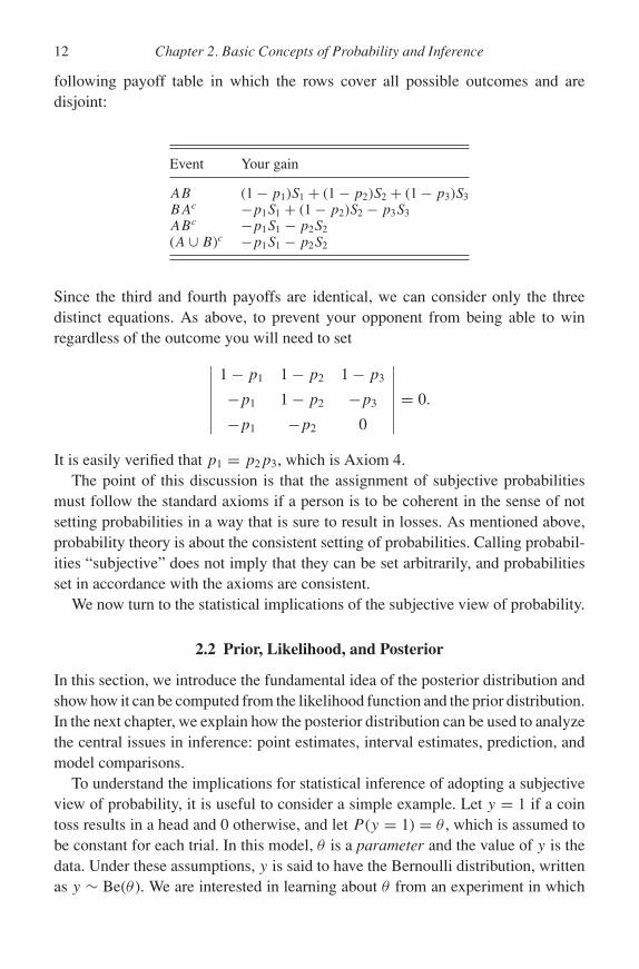
following payoff table in which the rows cover all possible outcomes and aredisjoint:

Event Your gain

AB (1 − p1)S1 + (1 − p2)S2 + (1 − p3)S3BAc −p1S1 + (1 − p2)S2 − p3S3ABc −p1S1 − p2S2(A ∪ B)c −p1S1 − p2S2

Since the third and fourth payoffs are identical, we can consider only the threedistinct equations. As above, to prevent your opponent from being able to winregardless of the outcome you will need to set∣∣∣∣∣∣∣

1 − p1 1 − p2 1 − p3

−p1 1 − p2 −p3

−p1 −p2 0

∣∣∣∣∣∣∣ = 0.

It is easily verified that p1 = p2p3, which is Axiom 4.The point of this discussion is that the assignment of subjective probabilities

must follow the standard axioms if a person is to be coherent in the sense of notsetting probabilities in a way that is sure to result in losses. As mentioned above,probability theory is about the consistent setting of probabilities. Calling probabil-ities “subjective” does not imply that they can be set arbitrarily, and probabilitiesset in accordance with the axioms are consistent.

We now turn to the statistical implications of the subjective view of probability.

2.2 Prior, Likelihood, and Posterior

In this section, we introduce the fundamental idea of the posterior distribution andshow how it can be computed from the likelihood function and the prior distribution.In the next chapter, we explain how the posterior distribution can be used to analyzethe central issues in inference: point estimates, interval estimates, prediction, andmodel comparisons.

To understand the implications for statistical inference of adopting a subjectiveview of probability, it is useful to consider a simple example. Let y = 1 if a cointoss results in a head and 0 otherwise, and let P (y = 1) = θ , which is assumed tobe constant for each trial. In this model, θ is a parameter and the value of y is thedata. Under these assumptions, y is said to have the Bernoulli distribution, writtenas y ∼ Be(θ ). We are interested in learning about θ from an experiment in which

P1: KAE


2.2 Prior, Likelihood, and Posterior 13

the coin is tossed n times yielding the data y = (y1, y2, . . . , yn), where yi indicateswhether the ith toss resulted in a head or tail.

From the frequentist point of view, probability theory can tell us something aboutthe distribution of the data for a given θ because the data can be regarded as the out-come of a large number of repetitions of tossing a coin n times. The parameter θ isan unknown number between zero and one. It is not given a probability distributionof its own, because it is not regarded as being the outcome of a repeated experiment.

From the subjective point of view, however, θ is an unknown quantity. Since thereis uncertainty over its value, it can be regarded as a random variable and assigneda probability distribution. Before seeing the data, it is assigned a prior distributionπ (θ ), 0 ≤ θ ≤ 1. Bayesian inference centers on the posterior distribution π (θ |y),which is the distribution of the random variable θ , conditioned on having observedthe data y. Note that in the coin-tossing example, the data yi are discrete – each is0 or 1 – but the parameter θ is continuous.

All the models we consider in this book have one or more parameters, and animportant goal of statistical inference is learning about their values. When there ismore than one parameter, the posterior distribution is a joint distribution of all theparameters, conditioned on the observed data. This complication is taken up in thenext chapter.

Before proceeding, we explain some conventions about notation fordistributions.

Notation for Density and Distribution Functions

• π (·) denotes a prior and π (·|y) denotes a posterior density function of parameters;these densities are continuous random variables in the statistical models we discuss.

• p(·) denotes the probability mass function (p.m.f.) of a discrete random variable;P (A) denotes the probability of event A.

• f (·) denotes the probability density function (p.d.f.) for continuous data. F (·) denotesthe (cumulative) distribution function (d.f.) for continuous data; that is, F (y0) =P (Y ≤ y0).

• When the distinction between discrete and continuous data is not relevant, we employthe f (·) notation for both probability mass and density functions.

The posterior density function π (θ |y) is computed by Bayes theorem, whichfollows from Axiom 4: from P (A|B) = P (AB)/P (B), we can infer P (B|A) =P (BA)/P (A). But since P (AB) = P (BA), we have Bayes theorem:

P (A|B) = P (B|A)P (A)

P (B).

P1: KAE



By setting A = θ and B = y, we have for discrete y

π (θ |y) = p(y|θ )π (θ )

p(y), (2.1)

where p(y) = ∫p(y|θ )π (θ ) dθ . The effect of dividing by p(y) is to make π (θ |y)

a normalized probability distribution: integrating Equation (2.1) with respect to θ

yields∫

π (θ |y) dθ = 1, as it should.For continuous or general y, we rewrite (2.1) as

π (θ |y) = f (y|θ )π (θ )

f (y), (2.2)

where f (y) = ∫f (y|θ )π (θ ) dθ . Equation (2.2) is the basis of Bayesian statistics

and econometrics. It is necessary to understand it thoroughly. The left-hand sidehas been interpreted as the posterior density function of θ |y. Now consider theright-hand side. The first term in the numerator is f (y|θ ), the density function forthe observed data y when the parameter value is θ . Take the coin-tossing experimentas an example. Suppose the coin is tossed three times and (H, T , H ) results, sothat y = (1, 0, 1). If the probability of a head is θ ,

P (1, 0, 1|θ ) = P (1|θ )P (0|θ )P (1|θ ) = θ (1 − θ )θ = θ2(1 − θ ).

From this expression, and in general, we see that f (y|θ ) is a function of θ oncethe data are known. As a function of θ , f (y|θ ) is called the likelihood function;it plays a central role in both frequentist and Bayesian statistics. It is important tonote that the likelihood function is not a p.d.f. for θ ; in particular, its integral overθ is not equal to one, although its integral (in this case, a sum) over y is.

The second term in the numerator of (2.2), the prior density π (θ ), embodies ourbeliefs about the distribution of θ before seeing the data y. These beliefs are basedon the researcher’s knowledge of the problem at hand; they may be based on theo-retical considerations or on previous empirical work. The prior distribution usuallydepends on parameters, called hyperparameters, which may either be supplied bythe researcher or given probability distributions.

We have already remarked that the denominator of (2.2), f (y), normalizes theposterior distribution. Since it is independent of θ , however, it is often convenientto write the posterior distribution as

π (θ |y) ∝ f (y|θ )π (θ ), (2.3)

that is, the posterior distribution is proportional to the likelihood function times theprior distribution. In this form, the right side of the equation does not integrate toone, but as a function of θ , it has the same shape as π (θ |y).

P1: KAE



For the Bayesian, the posterior distribution is central to inference because itcombines in one expression all the information we have about θ . It includes in-formation about θ before the current data through the prior distribution and theinformation contained in the current data through the likelihood function.

It is useful to think of (2.3) as a method of updating information, an idea thatis reinforced by the prior–posterior terminology. Before collecting the data y, ourinformation about θ is summarized by the prior distribution π (θ ). After observingy, our information about θ is summarized by the posterior distribution π (θ |y).Equation (2.3) tells us how to update beliefs after receiving new data: multiply theprior by the likelihood to find an expression proportional to the posterior.

We illustrate these ideas with the coin-tossing example. The likelihood functionfor a single toss of a coin can be written as p(yi |θ ) = θyi (1 − θ )1−yi , which impliesP (yi = 1|θ ) = θ and P (yi = 0|θ ) = 1 − θ . For n independent tosses of a coin, wetherefore have

p(y1, . . . , yn|θ ) = θy1 (1 − θ )1−y1 · · · θyn(1 − θ )1−yn

=∏

θyi (1 − θ )1−yi

= θ∑

yi (1 − θ )n−∑ yi . (2.4)

To complete the specification of the model, we need a prior distribution. Since0 ≤ θ ≤ 1, the prior should allow θ to take on any value in that interval and notallow it to fall outside that interval. A common choice is the beta distributionBeta(α, β) discussed in Section A.1.9:

π (θ ) = �(α + β)

�(α)�(β)θα−1(1 − θ )β−1, 0 ≤ θ ≤ 1, α, β > 0.

Note that α and β are hyperparameters. Why choose the beta distribution? First, itis defined in the relevant range. Second, it is capable of producing a wide varietyof shapes, some of which are displayed in Figure 2.1. Depending on the choice ofα and β, this prior can capture beliefs that indicate θ is centered at 1/2, or it canshade θ toward zero or one; it can be highly concentrated, or it can be spread out;and, when both parameters are less than one, it can have two modes.

The shape of a beta distribution can be understood by examining its mean andvariance:

E(θ ) = α

α + β, Var(θ ) = αβ

(α + β)2(α + β + 1).

From these expressions you can see that the mean is 1/2 if α = β, a larger α (β)shades the mean toward 1 (0), and the variance decreases as α or β increases. It isalso useful to note that we may first specify E(θ ), and Var(θ ) and then find the α

and β that correspond to the moments. These relationships may be found in (A.7).

P1: KAE



0 0.2 0.4 0.6 0.8 10

2

4

6

α = 0.5, β = 0.5

0 0.2 0.4 0.6 0.8 10

2

4

6

α = 1, β = 1

0 0.2 0.4 0.6 0.8 10

2

4

6

α = 5, β = 5

0 0.2 0.4 0.6 0.8 10

2

4

6

α = 30, β = 30

0 0.2 0.4 0.6 0.8 10

2

4

6

α = 10, β = 5

0 0.2 0.4 0.6 0.8 10

2

4

6

α =1, β = 30

Figure 2.1. Beta distributions for various values of α and β.

A third reason for choosing this distribution is that the beta prior in combinationwith the likelihood function of (2.4) yields a posterior distribution that has astandard form, which is convenient for analyzing the properties of the posterior.In fact, we next show that the posterior distribution for a model in which dataare generated by the Bernoulli distribution with a Beta(α0, β0) prior is also a betadistribution. This is an example of a conjugate prior, where the posterior distributionis in the same family as the prior distribution. From (2.3),

π (θ |y) ∝ p(y|θ )π (θ )

∝ θ∑

yi (1 − θ )n−∑ yi θα0−1(1 − θ )β0−1

∝ θ (α0+∑ yi )−1(1 − θ )(β0+n−∑ yi )−1.

In this expression, the normalizing constant of the beta distribution has been ab-sorbed into the proportionality constant because the constant does not dependon θ . As promised, π (θ |y) is in the form of a beta distribution with parametersα1 = α0 +∑ yi and β1 = β0 + n −∑ yi .

P1: KAE



The way in which α0 and β0 enter this expression is useful in interpreting theseparameters and in determining the values to assign to them. Note that α0 is added to∑

yi , the number of heads. This means that α0 can be interpreted as “the number ofheads obtained in the experiment on which the prior is based.” If, for example, youhad seen this coin tossed a large number of times and heads appeared frequently,you would set a relatively large value for α0. Similarly, β0 represents the numberof tails in the “experiment” on which the prior is based. Setting α0 = 1 = β0 yieldsthe uniform distribution. This prior indicates that you are sure that both a headand tail can appear but otherwise have no strong opinion about the distributionof θ . Choosing α0 = 0.5 = β0 yields a bimodal distribution with considerableprobability around zero and one, indicating that you would not be surprised if thecoin were two-headed or two-tailed.

It is easy to compute the mean of the posterior distribution from the propertiesof the beta distribution:

E(θ |y) = α1

α1 + β1

= α0 +∑ yi

α0 + β0 + n

=(

α0 + β0

α0 + β0 + n

)α0

α0 + β0+(

n

α0 + β0 + n

)y,

(2.5)

where y = (1/n)∑

yi . The last line expresses E(θ |y) as a weighted average of theprior mean α0/(α0 + β0) and the maximum likelihood estimator (MLE) y; that is, yis the value of θ that maximizes p(y|θ ). This result shows how the prior distributionand the data contribute to determine the mean of the posterior distribution. It is agood illustration of the way Bayesian inference works: the posterior distributionsummarizes all available information about θ , both from what was known beforeobtaining the current data and from the current data y.

As the sample size n becomes large, the weight on the prior mean approacheszero, and the weight on the MLE approaches one, implying that E(θ |y) → y.This is an example of a rather general phenomenon: the prior distribution be-comes less important in determining the posterior distribution as the sample sizeincreases. We graph in Figure 2.2 the prior, likelihood, and posterior for the casesn = 10,

∑yi = 3, α0 = 2, β0 = 2 and n = 50,

∑yi = 15, α0 = 2, β0 = 2. (The

likelihood has been normalized to integrate to one for easier comparison with theprior and posterior.) You can see how the larger sample size of the second example,reflected in the tighter likelihood function, causes the posterior to move furtheraway from the prior and closer to the likelihood function than when n = 10.

P1: KAE



0 0.1 0.2 0.3 0.4 0.5 0.6 0.7 0.8 0.9 1

1

3

5

7

n = 10, Σ yi = 3

PriorLikelhoodPosterior

0 0.1 0.2 0.3 0.4 0.5 0.6 0.7 0.8 0.9 1

1

3

5

7

n = 50, Σ yi = 15

PriorLikelhoodPosterior

Figure 2.2. Prior, likelihood, and posterior for coin-tossing example.

Although the preceding discussion shows that the beta prior is a “natural” priorfor Bernoulli data and that the choice of the two parameters in the beta prior cancapture a wide variety of prior beliefs, it is important to note that it is not necessaryto adopt a beta prior if no combination of parameters can approximate the prioryou wish to specify. Beta priors, for example, do not easily accommodate bimodaldistributions. We describe methods later in the book that can approximate theposterior distribution for any specified prior, even if the prior information does notlead to a posterior distribution of a standard form.

2.3 Summary

In this chapter, we first showed that subjective probabilities must satisfy the standardaxioms of probability theory if you wish to avoid losing a bet regardless of theoutcome. Having established that subjective probabilities must satisfy the usualaxioms of probability theory and, therefore, the theorems of probability theory, wederived the fundamental result of Bayesian inference: the posterior distribution ofa parameter is proportional to the likelihood function times the prior distribution.

P1: KAE


2.5 Exercises 19

2.4 Further Reading and References

Section 2.1.2 Excellent discussions of subjective probability may be found inHowson and Urbach (1993) and Hacking (2001).

2.5 Exercises

2.1 Prove the theorem P (A ∪ B) = P (A) + P (B) − P (AB) in two ways. First, write A ∪B = ABc ∪ AcB ∪ AB, and then use A = ABc ∪ AB and B = AB ∪ AcB. Second,apply coherency to a betting scheme like those in Section 2.1.2, where the four possibleoutcomes are ABc, AcB, AB, and (A ∪ B)c, and the bets, prices, and stakes are(A,p1, S1), (B,p2, S2), (AB,p3, S3), and (A ∪ B,p4, S4), respectively.

2.2 The Poisson distribution has probability mass function

p(yi |θ ) = θyi e−θ

yi!, θ > 0, yi = 0, 1, . . . ,

and let y1, . . . , yn be a random sample from this distribution.(a) Show that the gamma distribution G(α, β) is a conjugate prior distribution for the

Poisson distribution.(b) Show that y is the MLE for θ .(c) Write the mean of the posterior distribution as a weighted average of the mean of

the prior distribution and the MLE.(d) What happens to the weight on the prior mean as n becomes large?

2.3 The density function of the exponential distribution is

f (yi |θ ) = θe−θyi , θ > 0, yi > 0,

and let y1, . . . , yn be a random sample from this distribution.(a) Show that the gamma distribution G(α, β) is a conjugate prior distribution for the

exponential distribution.(b) Show that 1/y is the MLE for θ .(c) Write the mean of the posterior distribution as a weighted average of the mean of

the prior distribution and the MLE.(d) What happens to the weight on the prior mean as n becomes large?

2.4 Consider the uniform distribution with density function f (yi |θ ) = 1/θ , 0 ≤ yi ≤ θ ,and θ unknown.(a) Show that the Pareto distribution,

π (θ ) ={

akaθ−(a+1), θ ≥ k, a > 0,

0, otherwise,

is a conjugate prior distribution for the uniform distribution.(b) Show that θ = max(y1, . . . , yn) is the MLE of θ , where the yi are a random sample

from f (yi |θ ).(c) Find the posterior distribution of θ and its expected value.

P1: KAE


Chapter 3

Posterior Distributions and Inference

The first section of this chapter discusses general properties of posterior distri-butions. It continues with an explanation of how a Bayesian statistician uses theposterior distribution to conduct statistical inference, which is concerned withlearning about parameter values either in the form of point or interval estimates,making predictions, and comparing alternative models.

3.1 Properties of Posterior Distributions

In this section, we discuss general properties of posterior distributions, startingwith the choice of the likelihood function. We continue by generalizing the conceptto include models with more than one parameter and go on to discuss the revisionof posterior distributions as more data become available, the role of the samplesize, and the concept of identification.

3.1.1 The Likelihood Function

As we have seen, the posterior distribution is proportional to the product of the like-lihood function and the prior distribution. The latter is somewhat controversial andis discussed in Chapter 4, but the choice of a likelihood function is also an importantmatter and requires discussion. A central issue is that the Bayesian must specifyan explicit likelihood function to derive the posterior distribution. In some cases,the choice of a likelihood function appears straightforward. In the coin-tossingexperiment of Section 2.2, for example, the choice of a Bernoulli distributionseems natural, but it does require the assumptions of independent trials and aconstant probability. These assumptions might be considered prior information,but they are conventionally a part of the likelihood function rather than of the priordistribution.

20

P1: KAE


3.1 Properties of Posterior Distributions 21

In other cases, it may be more difficult to find a natural choice for the likelihoodfunction. The normal linear regression model, discussed in detail later, is a goodexample. A special case is the simple model

yi = µ + ui, ui ∼ N(0, σ 2), i = 1, . . . , n.

In this model, there are n independent observations on a variable y, which isassumed to be normally distributed with mean µ and variance σ 2. E. T. Jaynesoffers arguments for adopting the normal distribution when little is known aboutthe distribution. He takes the position that it is a very weak assumption in the sensethat it maximizes the uncertainty of the distribution of yi , where uncertainty ismeasured by entropy. Others argue that the posterior distribution may be highlydependent on the choice of a likelihood function and are not persuaded by Jaynes’sarguments. For example, a Student-t distribution with small degrees of freedomputs much more probability in the tail areas than does a normal distribution withthe same mean and variance, and this feature may be reflected in the posteriordistribution. Since for large degrees of freedom, there is little difference betweenthe normal and t distributions, a possible way to proceed is to perform the analysiswith several degrees of freedom and choose between them on the basis of posteriorodds ratios (see Section 3.2.4). In addition, distributions more general than thenormal and t may be specified; see Section 8.3 for further references.

Distributional assumptions also play a role in the frequentist approach to sta-tistical inference. A commonly used estimator in the frequentist literature is theMLE, which requires a specific distribution. Accordingly, a frequentist statisticianwho employs that method must, like a Bayesian, specify a distribution. Of course,the latter is also required to specify a prior distribution. Other approaches usedby frequentist econometricians, such as the generalized method of moments, donot require an explicit distribution. But, since the finite-sample properties of suchmethods are rarely known, their justification usually depends on a large-sampleproperty such as consistency, which is invoked even with small samples. Althoughthis type of analysis is more general than is specifying a particular distribution, theassumptions required to derive large-sample properties are often very technical anddifficult to interpret. The limiting distribution may also be a poor approximationto the exact distribution. In contrast, the Bayesian approach is more transparentbecause a distributional assumption is explicitly made, and Bayesian analysis doesnot require large-sample approximations.

To summarize:

• The assumed form of the likelihood function is a part of the prior information and requiressome justification, and it is possible to compare distributional assumptions with the aidof posterior odds ratios if there is no clear choice on a priori grounds.

P1: KAE


22 Chapter 3. Posterior Distributions and Inference

• Several families of distributions can be specified and analyzed with the tools discussedin Parts II and III.

3.1.2 Vectors of Parameters

The single-parameter models we have studied thus far are now generalized to amodel with d parameters contained in the vector θ = (θ1, θ2, . . . , θd). The previousdefinitions of likelihood, prior, and posterior distributions still apply, but they arenow, respectively, the joint likelihood function, joint prior distribution, and jointposterior distribution of the multivariate random variable θ .

From the joint distributions, we may derive marginal and conditional distri-butions according to the usual rules of probability. Suppose, for example, we areprimarily interested in θ1. The marginal posterior distribution of θ1 can be found byintegrating out the remainder of the parameters from the joint posterior distribution:

π (θ1|y) =∫

π (θ1, . . . , θd |y) dθ2 . . . dθd.

It is important to recognize that the marginal posterior distribution is different fromthe conditional posterior distribution. The latter is given by

π (θ1|θ2, . . . , θd, y) = π (θ1, θ2, . . . , θd |y)

π (θ2, . . . , θd |y),

where the denominator on the right-hand side is the marginal posterior distributionof (θ2, . . . , θd) obtained by integrating θ1 from the joint distribution. In most appli-cations, the marginal distribution of a parameter is more useful than its conditionaldistribution because the marginal takes into account the uncertainty over the valuesof the remaining parameters, while the conditional sets them at particular values.To see this, write the marginal distribution as

π (θ1|y) =∫

π (θ1|θ2, . . . , θd, y)π (θ2, . . . , θd |y) dθ2 . . . dθd.

In this form, we see that all values of θ2, . . . , θd contribute to the determinationof π (θ1|y) in proportion to their probabilities computed from π (θ2, . . . , θd |y). Inother words, the marginal distribution π (θ1|y) is an average of the conditionaldistributions π (θ1|θ2, . . . , θd, y), where the conditioning values (θ2, . . . , θd) areweighted by their posterior probabilities.

In some cases, it may be of interest to examine the marginal distribution oftwo parameters, say, θ1 and θ2. This may be found as above by integrating out theremaining parameters. The resulting distribution is a joint distribution because itinvolves two variables, and it is a marginal distribution because it is determinedby integrating out the variables θ3, . . . , θd . It is thus a joint marginal posterior

P1: KAE



distribution, but it is called a marginal posterior distribution. While the marginalposterior distributions for any number of parameters can be defined, attentionis usually focused on one- or two-dimensional distributions because these can bereadily graphed and understood. Joint distributions in higher dimensions are usuallydifficult to summarize and comprehend.

Although it is easy to write down the definition of the marginal posterior distri-bution, performing the necessary integration to obtain it may be difficult, especiallyif the integral is not of a standard form. Parts II and III of this book are concernedwith the methods of approximating such nonstandard integrals, but we now discussan example in which the integral can be computed analytically.

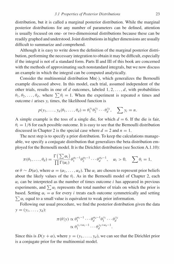
Consider the multinomial distribution Mn(·), which generalizes the Bernoulliexample discussed above. In this model, each trial, assumed independent of theother trials, results in one of d outcomes, labeled 1, 2, . . . , d, with probabilitiesθ1, θ2, . . . , θd, where

∑θi = 1. When the experiment is repeated n times and

outcome i arises yi times, the likelihood function is

p(y1, . . . , yd |θ1, . . . , θd) = θy11 θ

y22 · · · θyd

d ,∑

yi = n.

A simple example is the toss of a single die, for which d = 6. If the die is fair,θi = 1/6 for each possible outcome. It is easy to see that the Bernoulli distributiondiscussed in Chapter 2 is the special case where d = 2 and n = 1.

The next step is to specify a prior distribution. To keep the calculations manage-able, we specify a conjugate distribution that generalizes the beta distribution em-ployed for the Bernoulli model. It is the Dirichlet distribution (see Section A.1.10):

π (θ1, . . . , θd) = �(∑

αi

)∏�(αi)

θα1−11 θ

α2−12 · · · θαd−1

d , αi > 0,∑

θi = 1,

or θ ∼ D(α), where α = (α1, . . . , αd). The αi are chosen to represent prior beliefsabout the likely values of the θi . As in the Bernoulli model of Chapter 2, eachαi can be interpreted as the number of times outcome i has appeared in previousexperiments, and

∑αi represents the total number of trials on which the prior is

based. Setting αi = α for every i treats each outcome symmetrically and setting∑αi equal to a small value is equivalent to weak prior information.Following our usual procedure, we find the posterior distribution given the data

y = (y1, . . . , yd):

π (θ |y) ∝ θα1−11 · · · θαd−1

d θy11 · · · θyd

d

∝ θy1+α1−11 · · · θyd+αd−1

d .

Since this is D(y + α), where y = (y1, . . . , yd), we can see that the Dirichlet prioris a conjugate prior for the multinomial model.

P1: KAE



We can now find the marginal distribution for any of the θi , for example, θ1.From the result given in Section A.1.10,

π (θ1|y) ∝ Beta

(y1 + α1,

∑i =1

(yi + αi)

),

which is a beta distribution. In the die-throwing example, the probability of the 1spot appearing when a single die is thrown is given by the beta distribution:

θ1 ∼ Beta

(y1 + α1,

6∑i=2

(yi + αi)

).

Note that this result is equivalent to considering the 1-spot as one outcome and theother die faces as a second outcome, transforming the multinomial model into abinomial model.

To summarize, when dealing with a model that contains more than one pa-rameter, simply redefine the parameter as a vector. Then, all the definitions andconcepts discussed in Section 2.1.2 apply to the vector of parameters. In addition,the marginal and conditional distributions of individual parameters or groups ofparameters can be found by applying the usual rules of probability.

3.1.3 Bayesian Updating

This section explains a very attractive feature of Bayesian inference – the way inwhich posterior distributions are updated as new information becomes available.Let θ represent one parameter or a vector of parameters, and let y1 represent thefirst set of data obtained in an experiment. As an example, you may think of y1

as the number of heads found in tossing a coin n1 times, where the probability ofheads is θ . As usual,

π (θ |y1) ∝ f (y1|θ )π (θ ).

Next, suppose that a new set of data y2 is obtained, and we wish to compute theposterior distribution given the complete data set π (θ |y1, y2). By the usual rules ofprobability,

π (θ |y1, y2) ∝ f (y1, y2|θ )π (θ )

= f (y2|y1, θ )f (y1|θ )π (θ )

= f (y2|y1, θ )π (θ |y1). (3.1)

If the data sets are independent, f (y2|y1, θ ) simplifies to f (y2|θ ).Whether or not the data sets are independent, however, note that (3.1) has the

form of a likelihood times a density for θ , but that the latter density is π (θ |y1): the

P1: KAE



posterior distribution based on the initial set of data occupies the place where a priordistribution is expected. It is now easy to verify that, if more new data y3 becomeavailable, π (θ |y1, y2, y3) has π (θ |y1, y2) where you would expect to see π (θ ). Thus,as new information is acquired, the posterior distribution becomes the prior for thenext experiment. In this way, the Bayesian updates the prior distribution to reflectnew information. It is important to emphasize that this updating is a consequence ofprobability theory and requires no new principles or ad hoc reasoning. Updating alsojustifies our interpretation of the prior distribution as being based on previous data,if such data are available, or on the equivalent of previous data in the researcher’sview.

As a simple example of updating, consider data generated from the Bernoulliexample. Assume a beta prior with parameters α0 and β0. Suppose the first exper-iment produces n1 trials and set s1 = ∑

y1i ; let the second experiment producen2 trials and set s2 = ∑

y2i . We can then compute the posterior based on the firstexperiment as

f (θ |s1) ∝ θα0−1(1 − θ )β0−1θs1 (1 − θ )n1−s1,

or

θ |s1 ∼ Beta(α0 + s1, β0 + (n1 − s1)).

If we take the latter as the prior for the second experiment, we find

f (θ |s1, s2) ∝ θα0+s1 (1 − θ )β0+(n1−s1)θs2 (1 − θ )n2−s2,

or

θ |s1, s2 ∼ Beta(α0 + (s1 + s2), β0 + (n1 + n2) − (s1 + s2)).

The latter distribution is implied by a Beta(α0, β0) prior and obtaining s1 + s2 oneson n1 + n2 trials.

To summarize, when data are generated sequentially, the Bayesian paradigmshows that the posterior distribution for the parameter based on new evidenceis proportional to the likelihood for the new data, given previous data and theparameter, times the posterior distribution for the parameter, given the earlier data.This is an intuitively reasonable way of allowing new information to influencebeliefs about a parameter, and it appears as a consequence of standard probabilitytheory.

3.1.4 Large Samples

Although the concepts of Bayesian inference hold true for any sample size, itis instructive to examine how the posterior distribution behaves in large samples.

P1: KAE



This analysis offers important insights about the nature of the posterior distribution,particularly about the relative contributions of the prior distribution and likelihoodfunction in determining the posterior distribution.

Consider the case of independent trials, where the likelihood function L(θ |y) is

L(θ |y) =∏

f (yi |θ )

=∏

L(θ |yi);

L(θ |yi) is the likelihood contribution of yi . Also define the log likelihood functionl(θ |y) as

l(θ |y) = log L(θ |y)

=∑

l(θ |yi)

= nl(θ |y),

where l(θ |yi) is the log likelihood contribution of yi and l(θ |y) = (1/n)∑

l(θ |yi)is the mean log likelihood contribution.

The posterior distribution can be written as

π (θ |y) ∝ π (θ )L(θ |y)

∝ π (θ ) exp[nl(θ |y)].

We can now examine the effect of the sample size n on the posterior distribution,which is proportional to the product of the prior distribution and a term thatinvolves an exponential raised to n times a number. For large n, the exponentialterm dominates π (θ ), which does not depend on n. Accordingly, we can expectthat the prior distribution will play a relatively smaller role than do the data, asreflected in the likelihood function, when the sample size is large. Conversely, theprior distribution has relatively greater weight when n is small.

As an example of this phenomenon, recall the coin-tossing example ofSection 2.2. It was shown that

E(θ |y) =(

α + β

α + β + n

)α

α + β+(

n

α + β + n

)y,

which is a weighted average of the mean of the prior α/(α + β) and the samplemean y. For large n, the weight of the prior mean is small compared to that of thesample mean.

This idea can be taken one step further. If we denote the true value of θ by θ0, itcan be shown that

limn→∞ l(θ |y) → l(θ0|y).

P1: KAE



Accordingly, for large n, the posterior distribution collapses to a distribution withall its probability at θ0. This property is similar to the criterion of consistency inthe frequentist literature and extends to the multiparameter case.

Finally, we can use these ideas to say something about the form of the posteriordistribution for large n. To do this, take a second-order Taylor series approximationof l(θ |y) around θ , the MLE of θ :

l(θ |y) ≈ l(θ |y) − n

2(θ − θ )2[−l′′(θ |y)]

= l(θ |y) − n

2v(θ − θ )2,

where l′′(θ |y) = (1/n)∑

k l′′(θ |yk) and v = [−l′′(θ |y)]−1. The term involvingthe first derivative l′(θ |y) vanishes because l(θ |y) is maximized at θ = θ , andl′′(θ |y) < 0 for the same reason. The posterior distribution can therefore be writtenapproximately as

π (θ |y) ∝ π (θ ) exp[− n

2v(θ − θ )2

].

The second term is in the form of a normal distribution with mean θ and variancev/n, and it dominates π (θ ) because of the n in the exponential. If π (θ) = 0, π (θ |y)is approximately a normal distribution with mean θ for large n.

The requirement that π (θ ) does not vanish at θ should be stressed. It is interpretedas a warning that the prior distribution should not be specified so as to rule outvalues of θ that are logically possible. Such values of θ may be strongly favoredby the likelihood function, but would have zero posterior probability if π (θ) = 0.

In the multiparameter case, the second-order Taylor series is

l(θ |y) ≈ l(θ |y) − n

2(θ − θ)′[−l′′(θ |y)](θ − θ)

= l(θ |y) − n

2(θ − θ)′V −1(θ − θ), (3.2)

where l′′(θ |y) = (1/n)∑

k{ ∂2l(θ |yk)∂θi∂θj

} is the mean of the matrix of second derivatives

of the log likelihood evaluated at the MLE and V = [−l′′(θ |y)]−1. For large n, wecan therefore approximate π (θ |y) by a multivariate normal distribution with meanθ and covariance matrix (1/n)V .

In summary, when n is large, (1) the prior distribution plays a relatively small rolein determining the posterior distribution, (2) the posterior distribution converges toa degenerate distribution at the true value of the parameter, and (3) the posteriordistribution is approximately normally distributed with mean θ .

P1: KAE



3.1.5 Identification

In this section we discuss the idea of identification and the nature of the poste-rior distribution for unidentified parameters. Our starting point is the likelihoodfunction, which is also used by frequentist statisticians to discuss the concept. Todefine identification, we suppose that there are two different sets of parameters θ

and ψ such that f (y|θ ) = f (y|ψ) for all y. In that case, the two models are said tobe observationally equivalent. This means that the observed data could have beengenerated by the model with parameter vector θ or by the model with parametervector ψ , and the data alone cannot determine which set of parameters generatedthe data. The model or the parameters of the model are not identified or unidentifiedwhen two or more models are observationally equivalent. The model is identified(or the parameters are identified) if no model is observationally equivalent to themodel of interest.

A special case of nonidentifiability arises when f (y|θ1, θ2) = f (y|θ1). In thatcase, the parameters in θ2 are not identified. A familiar example of this situation andhow to deal with it is the specification of a linear regression model with a dummy(or indicator) variable. It is well known that a complete set of dummy variablescannot be included in a model along with a constant, because the set of dummiesand the constant are perfectly correlated; this is a symptom of the nonidentifiabilityof the constant and the coefficients of a complete set of dummies. The problem issolved by dropping either one of the dummies or the constant.

The discussion of identification to this point has been based on the specificationof the likelihood function, what we might call “identification through the data,”but the Bayesian approach also utilizes a prior distribution. Consider the likelihoodfunction f (y|θ1, θ2) = f (y|θ1). It is clear that the data have no information aboutθ2 when θ1 is given, but what can be said about the posterior distribution π (θ2|y)?Although we might expect that it is equal to π (θ2) since the data contain noinformation about θ2, consider the following calculation:

π (θ2|y) =∫

π (θ1, θ2|y) dθ1

=[ ∫

f (y|θ1, θ2)π (θ1)π (θ2|θ1) dθ1

]/f (y)

=[ ∫

f (y|θ1)π (θ1)π (θ2|θ1) dθ1

]/f (y)

=∫

π (θ1|y)π (θ2|θ1) dθ1.

If the prior distribution of θ2 is independent of θ1, that is, π (θ2|θ1) = π (θ2), thenπ (θ2|y) = π (θ2), implying that knowledge of y does not modify beliefs about θ2.

P1: KAE


3.2 Inference 29

But if the two sets of parameters are not independent in the prior distribution,information about y modifies beliefs about θ2 by modifying beliefs about θ1.

This last result is the main point of our discussion of identification: since thedata are only indirectly informative about unidentified parameters – any differencebetween their prior and posterior distributions is due to the nature of the priordistribution – inferences about such parameters may be less convincing than areinferences about identified parameters. A researcher should know whether theparameters included in a model are identified through the data or through the priordistribution when presenting and interpreting posterior distributions.

There are some situations when it is convenient to include unidentified param-eters in a model. Examples of this practice are presented at several places later inthe book, where the lack of identification will be noted.

3.2 Inference

We now show how the posterior distribution serves as the basis for Bayesianstatistical inference.

3.2.1 Point Estimates

Suppose that the model contains a scalar parameter θ that we wish to estimate. TheBayesian approach to this problem uses the idea of a loss function L(θ , θ ). Thisfunction specifies the loss incurred if the true value of the parameter is θ , but it isestimated as θ . Examples are the absolute value loss function L1(θ , θ ) = |θ − θ |,the quadratic loss function L2(θ , θ ) = (θ − θ )2, and the bilinear loss function

L3(θ , θ ) ={

a|θ − θ |, for θ > θ,

b|θ − θ |, for θ ≤ θ ,

where a, b > 0. For these loss functions, loss is minimized if θ = θ , and increasesas the difference between θ and θ increases. The Bayes estimator of θ is the valueof θ that minimizes the expected value of the loss, where the expectation is takenover the posterior distribution of θ ; that is, θ is chosen to minimize

E[L(θ , θ )] =∫

L(θ , θ )π (θ |y) dθ.

Under quadratic loss, we minimize

E[L(θ , θ )] =∫

(θ − θ )2π (θ |y) dθ.

P1: KAE



This is easily done by differentiating the function with respect to θ and settingthe derivative equal to zero (it is assumed that the order of differentiation andintegration can be interchanged), yielding

2∫

(θ − θ )π (θ |y) dθ = 0,

or

θ =∫

θπ (θ |y) dθ.

From the last expression, we see that θ = E(θ |y): the optimal point estimator forθ under quadratic loss is the mean of the posterior distribution of θ . It is left for anexercise to derive the optimal estimators under the absolute value and bilinear lossfunctions. Another exercise considers a loss function that yields the mode of theposterior distribution as the optimal estimator.

It is enlightening to contrast the Bayesian approach to point estimation withthat of a frequentist statistician. The frequentist stipulates one or more criteria thatan estimator should satisfy and then attempts to determine whether a particularestimator satisfies those criteria. One such criterion is that of unbiasedness: anestimator θ , which is a function of the observed data, is unbiased for θ if E(θ) = θ .For many models, it is impossible to determine whether an estimator is unbiased;in such cases, a large-sample property, such as consistency, is often substituted.For other models, there is more than one unbiased estimator, and a criterion suchas efficiency is added to choose between them.

Although both frequentist and Bayesian approaches to point estimation involvean expected value, it is important to recognize that the expectations are takenover different probability distributions. The Bayesian calculation is taken over theposterior distribution of the parameter, which is conditioned on the observed datay. In contrast, the frequentist expectation to determine the expected value of anestimator is taken over the distribution of the estimator, which is conditioned onthe unknown parameter θ .

The coin-tossing example illustrates this difference. Consider the estimator θ =(1/n)

∑yi = y. To determine whether this estimator is unbiased, we find the

distribution of y, given the assumed Bernoulli model, and compute its expectedvalue over the distribution of y:

E(y) =∫

yf (y|θ ) dy.

This calculation considers every possible value of y, which arises from everypossible value of the data that might have been observed, not just the data that

P1: KAE


3.2 Inference 31

are actually observed. In contrast, Bayesian calculations are based on the posteriordistribution, which is conditioned only on data that have been observed.

There is another very important difference between the approaches. In the fre-quentist approach, it is necessary to propose one or more estimators that are thentested to see whether they satisfy the specified criteria. There is no general methodof finding candidates for estimators that are sure to satisfy such criteria. In con-trast, the Bayesian approach is mechanical: given a loss function, the problemis to find the estimator that minimizes expected loss. Under quadratic loss, forexample, it is necessary to find the mean of the posterior distribution. While thedetails of finding the mean may be difficult in some cases, the goal is clear. Itis not necessary to devise an estimator for every type of model that might beencountered.

3.2.2 Interval Estimates

In addition to reporting a point estimate of a parameter θ , it is often useful to reportan interval estimate of the form

P (θL ≤ θ ≤ θU ) = 0.95,

which tells us that θL ≤ θ ≤ θU with a probability of 0.95. Of course, 0.95 can bereplaced by another value. Bayesians call such intervals credibility intervals (orBayesian confidence intervals) to distinguish them from a quite different conceptthat appears in frequentist statistics, the confidence interval. For a Bayesian, valuesof θL and θU can be determined to obtain the desired probability from the posteriordistribution. If more than one pair is possible, the pair that results in the shortestinterval may be chosen; such a pair yields the highest posterior density interval(h.p.d.). This procedure is possible because probability statements can be madeabout the values of a parameter.

In contrast, frequentists define a confidence interval, which does not involvethe probability distribution of a parameter. As in the case of point estimators,this approach makes use of unobserved data. Consider, for example, a confidenceinterval for the mean µ of a N(µ, 1) distribution based on n observations. Theclaim that (x − 1.96/

√n, x + 1.96/

√n) is a 95% confidence interval for the mean

follows from the result that 95% of all possible sample means x lie in the interval(µ − 1.96/

√n, µ + 1.96/

√n). This calculation involves sample means that are

not observed. The Bayesian approach, based on the posterior distribution, con-ditions on the observed data points and does not make use of data that are notobserved.

P1: KAE



3.2.3 Prediction

Another basic issue in statistical inference is the prediction of new data values. Tofix ideas, consider the coin-tossing example. Suppose that the data y = (y1, . . . , yn)have been observed, and we wish to predict the outcome of the next toss, yn+1.From the Bayesian viewpoint, we can compute P (yn+1 = 1|y), the probability thatthe next toss results in a head, given the data previously observed; the probabilityof a tail is one minus this probability. We compute this probability by making useof the identity

P (yn+1 = 1|y) =∫

f (yn+1 = 1, θ |y) dθ

=∫

P (yn+1 = 1|θ, y)π (θ |y) dθ

=∫

P (yn+1 = 1|θ )π (θ |y) dθ.

Notice carefully what we have done. Following the rules of probability, we writeP (yn+1 = 1|y) as an integral in which θ is first introduced into and then integratedout of the joint density f (yn+1 = 1, θ |y). In the second line, the joint distribution iswritten as the product of a distribution conditioned on θ and y, P (yn+1 = 1|θ, y),and a distribution of θ conditioned on the previous data y, π (θ |y). In the third line,we drop y from the conditioning set of P (yn+1 = 1|θ, y) because of the assumptionof the Bernoulli model that the yi are independent given θ . The expressions in thelast line are the probability P (yn+1 = 1|θ ) and the posterior distribution of θ .You can think of computing this integral as repeating the following calculationa large number of times: first draw a value of θ from its posterior distributionπ (θ |y) and then compute P (yn+1 = 1|θ ) using this value of θ . The average ofthese probabilities is P (yn+1 = 1|y).

The general case has the same form. In predicting a new value of y, say yf ,whether θ is a scalar or a vector representing several parameters, we write

f (yf |y) =∫

f (yf |θ, y)π (θ |y) dθ,

where y is retained in the first expression under the integral to allow for thepossibility that yf is not independent of y. This situation arises in some models fortime series.

Consider prediction in the coin-tossing example. The posterior distribution of θ

is in the form of a beta distribution:

π (θ |y) = �(α1 + β1)

�(α1)�(β1)θα1−1(1 − θ )β1−1.

P1: KAE


3.2 Inference 33

Since P (yn+1 = 1|θ ) = θ , we have

P (yn+1 = 1|y) = �(α0 + β0 + n)

�(α0 +∑ yi)�(β0 + n −∑ yi)

×∫

θ θα0+∑ yi−1(1 − θ )β0+n−∑ yi−1 dθ

= �(α0 + β0 + n)

�(α0 +∑ yi)�(β0 + n −∑ yi)

×∫

θα0+∑ yi (1 − θ )β0+n−∑ yi−1 dθ

= �(α0 + β0 + n)

�(α0 +∑ yi)�(β0 + n −∑ yi)

× �(α0 +∑ yi + 1)�(β0 + n −∑ yi)

�(α0 + β0 + n + 1)

= α0 +∑ yi

α0 + β0 + n,

where we have used �(α) = (α − 1)�(α − 1). Since we found in (2.5) that

E(θ |y) = α0 +∑ yi

α0 + β0 + n,

our estimate of P (yn+1 = 1|y) is the mean of the posterior distribution of θ . Thisshould not be surprising, because, for a Bernoulli variable,

E(y|θ ) = P (y = 1|θ ) = θ.

3.2.4 Model Comparison

A fourth aspect of statistical inference is to determine which of the several compet-ing models is better supported by our information. Suppose that we wish to comparetwo models: Model 1, M1, consists of a prior probability P (M1) = p1 that M1 isthe true model, a set of parameters θ1, a prior for those parameters π1(θ1), and alikelihood function f1(y|θ1). Model 2, M2, consists of p2, θ2, π2(θ2), and f2(y|θ2).Two models may differ in their priors, their likelihoods, or their parameters. Inlinear regression, for example, two models might differ by which covariates areincluded, which corresponds to two different specifications of the parameter vectorθ . This difference also implies different priors and different likelihood functions.

The Bayesian approach to this inferential problem is to compute P (Mi |y),i = 1, 2, which is interpreted as “the probability that Model i is the correct model,given the data.” If we have only two models, then P (M2|y) = 1 − P (M1|y). Tocompute P (M1|y), use Bayes theorem and the approach taken in deriving the

P1: KAE



predictive distribution; that is, introduce the parameters and then integrate themout:

P (M1|y) = P (M1)f1(y|M1)

f (y)

= p1∫f1(y, θ1|M1) dθ1

f (y)

= p1∫f1(y|θ1, M1)π1(θ1|M1) dθ1

f (y),

where

f (y) = p1

∫f1(y|θ1, M1)π1(θ1|M1) dθ1 + p2

∫f2(y|θ2, M2)π2(θ2|M2) dθ2.

(3.3)Each term of f (y) is the integral of a likelihood function with respect to a priordistribution,

mi(y) =∫

fi(y|θi, Mi)πi(θi |Mi) dθi. (3.4)

It is called the marginal likelihood for model i and can be interpreted as theexpected value of the likelihood function with respect to the prior distribution.From the definition of the posterior distribution in (2.2),

π (θ |y) = f (y|θ )π (θ )

f (y)

= f (y|θ )π (θ )∫f (y|θ )π (θ ) dθ

,

we see that the marginal likelihood is equal to the inverse of the normalizingconstant of the posterior distribution. It is important to include the normalizingconstants of f (y|θ ) and π (θ ) when computing the marginal likelihood.

In comparing two models, it is often instructive to compute the odds ratio infavor of Model 1 over Model 2, given the data,

R12 = P (M1|y)

P (M2|y)

=(

p1

p2

)(∫f1(y|θ1, M1)π1(θ |M1) dθ1∫f2(y|θ2, M2)π2(θ |M2) dθ2

)=(

p1

p2

)(m1(y)

m2(y)

).

The first term on the right-hand side is the prior odds ratio, the ratio of the priorprobability of M1 to the prior probability of M2. The second term, the ratio of

P1: KAE


3.2 Inference 35

Table 3.1. Jeffreys Guidelines.

log10(R12) > 2 Decisive support for M13/2 < log10(R12) < 2 Very strong evidence for M11 < log10(R12) < 3/2 Strong evidence for M11/2 < log10(R12) < 1 Substantial evidence for M10 < log10(R12) < 1/2 Weak evidence for M1

the marginal likelihoods of the two models, is called the Bayes factor. Note thatf (y) of (3.3) has dropped out of this expression because it has the same valuefor both P (M1|y) and P (M2|y). A large value of R12 is evidence that M1 is bettersupported than is M2 by the data and the prior information, and a small value isevidence that M2 is better supported; values around 1 indicate that both models aresupported equally well. Such pairwise comparisons can also be made when thereare more than two models. It is convenient to present log10(R12) rather than R12

because the ratio is often very large or very small, and the logarithm to base 10is immediately interpreted as powers of 10. Table 3.1 presents guidelines for theinterpretation of log10(R12) suggested by Jeffreys (1961, p. 432). It should be clearthat these values are arbitrary, as is the 5% level of significance often employedby frequentist statisticians.

If you are reluctant to specify the prior odds ratio, the burden falls on theBayes factor to discriminate between models. If, for example, it is found thatlog10(R12) = 2, a value of p1/p2 less than 1/100 would be required to result in aposterior odds ratio in favor of M2. This indicates that the results favor M1 unlessyou think M1 to be very improbable a priori compared to M2.

Model choice can be implemented in terms of loss functions for making correctand incorrect choices, but, in practice, models are often informally comparedby their Bayes factors or their posterior odds ratios. One possible outcome ofsuch comparisons is that one or more models are effectively eliminated fromconsideration because other models have much greater support on the basis ofthese criteria. Another possibility is that several models that are not eliminatedhave pairwise Bayes factors or posterior odds ratios close to one (or zero on thelog scale). In this case, it would be reasonable to conclude that two or more modelsare consistent with the data and prior information and that a choice between themmust be delayed until further information becomes available.

When a prediction is to be made and more than one model is being considered,the technique of model averaging can be applied. If, for example, m models havebeen specified, a prediction may be formed as a weighted average of the predictions

P1: KAE



from each of the models under consideration:

f (yf |y) =m∑

i=1

p(Mi |y)fi(yf |y, Mi)

=m∑

i=1

p(Mi |y)∫

fi(yf |θi, y, Mi)πi(θi |y, Mi) dθi.

From this expression, you can see that models with small values of p(Mi |y)contribute little to predictions.

The frequentist approach to model comparison makes use of hypothesis tests.In this approach, the null hypothesis H0 is rejected in favor of the alternativehypothesis HA if the value of a statistic computed from the data falls in the criticalregion. The critical region is usually specified to set the probability that H0 isrejected when it is true at a small value, where the probability is computed overthe distribution of the statistic. As mentioned before, this calculation depends onvalues of the statistic that were not observed.

An important advantage of the Bayesian approach to model comparison over thefrequentist approaches is that the former can easily deal with nonnested hypotheses,especially with models that deal with different representations of the responsevariable. A common example is the choice between y and log(y) as the responsevariable. In general, suppose that under M1, the likelihood function is f1(y|θ1), andunder M2, it is f2(z|θ2), where z = g(y) and g′(y) = 0. Since y and g(y) containthe same information, the posterior odds ratio should not depend on whether wecompute

P (M1|y)/P (M2|y)

or

P (M1|z)/P (M2|z),

and it does not. Since, by the usual transformation of variables rule,

f (zi |θ ) = f (yi |θ )

∣∣∣∣dyi

dzi

∣∣∣∣ ,it is easy to see that the Bayes factor is independent of whether the responsevariable is y or z = g(y) because the Jacobian term cancels. Note also that thisresult generalizes to multivariate y and z, where the absolute value of the derivativeis replaced by the absolute value of the Jacobian of the transformation.

P1: KAE


3.2 Inference 37

It is instructive to examine the effect of the sample size on the Bayes factor.Exponentiate (3.2) and substitute into (3.4) to obtain

mi(y) ≈ Li(θi |y)∫

exp[−n

2(θi − θi)

′V −1i (θi − θi)

]πi(θi) dθi

≈ Li(θi |y)πi(θi)∫

exp[−n

2(θi − θi)

′V −1i (θi − θi)

]dθi,

where πi(θi) is approximated by πi(θi) because the exponential term dominates theintegral in the region around θi . The integration yields

mi(y) ≈ Li(θi |y)πi(θi)(2π )di/2|n−1Vi |1/2

≈ Li(θi |y)πi(θi)(2π )di/2n−di/2|Vi |1/2,

where di is the dimension of θi ; that is, the number of parameters in Mi . We cannow approximate the logarithm of the Bayes factor for comparing models 1 and 2:

log(B12) ≈[

log

(L1(θ1|y)

L2(θ2|y)

)− d1 − d2

2log(n)

]

+[

log

(π1(θ1)

π2(θ2)

)+ 1

2log

( |V1||V2|

)+ d1 − d2

2log(2π )

].

Since the second square-bracketed term does not depend on n, its importance maybe neglected for large n. The first term in the first square bracket is the logarithm ofthe likelihood ratio. It will tend to become large if M1 is the true model and smallif M2 is true. The second term shows that the log Bayes factor penalizes modelswith larger numbers of parameters, where the penalty is log(n) times the differencein the number of parameters divided by two.

We return to the coin-tossing example to illustrate the use of Bayes factors formodel comparison. To specify two competing models, consider the following vari-ation on our basic experiment. A coin is tossed m times by Michaela and then tossedm times by Lila. Suppose we believe it possible that the different ways in whichthe girls toss the coin result in different probabilities. Let θ1 be the probability of ahead when Michaela tosses the coin and θ2 = θ1 be the corresponding probabilitywhen Lila tosses it. We also consider a model in which there is no difference inthe probabilities. Specifically, θ1 = θ2 = θ in M1, and θ1 = θ2 in M2. To simplifycalculations, assume that π1(θ1) = Beta(1, 1) = π2(θ2). Verify that this choice of aprior implies π (θ ) = 1, 0 ≤ θ ≤ 1.

Let y1 be the proportion of heads when Michaela tosses the coin, y2 be Lila’sproportion, and y = (y1 + y2)/2 be the overall proportion. The marginal likelihood

P1: KAE



Table 3.2. Bayes Factors for Selected PossibleOutcomes

Michaela Lila log10(Bayes factor)

Proportion heads Proportion heads m = 10 m = 100

0.1 0.9 −2.506 −30.7750.2 0.8 −1.200 −15.7930.3 0.7 −0.348 −6.3160.4 0.6 0.138 −0.9750.5 0.5 0.297 0.756

under M1 is ∫θ2my(1 − θ )2m−2my = �(2my + 1)�(2m − 2my + 1)

�(2m + 2).

As an exercise, verify that the marginal likelihood under M2 is

�(my1 + 1)�(m − my1 + 1)

�(m + 2)

�(my2 + 1)�(m − my2 + 1)

�(m + 2). (3.5)

We list in Table 3.2 the log10(Bayes factors) for selected values of outcomes andfor two different sample sizes, 10 and 100. Note that the Bayes factor in favor ofM1 increases as the proportion of heads for both girls approaches 0.5. You can seethat M1 is decisively rejected when there are large differences between Michaela’sand Lila’s results and that results are much sharper for the larger sample size.

3.3 Summary

We began by exploring the posterior distribution in more detail. In particular,we considered models with more than one parameter, updating posterior distribu-tions as additional data become available, how the posterior distribution behavesas sample size increases, and the concept of identification. We then explainedhow posterior distributions can be used to find point and interval estimates, makepredictions, and compare the credibility of alternative models.


Section 3.1.1 Jaynes’s arguments may be found in Jaynes (2003, chap. 7). Zellnerhas proposed the Bayesian Method of Moments when there are difficulties in for-mulating a likelihood function. The method can be employed to compute postdatamoments of parameters and future values of variables without a likelihood function,

P1: KAE


3.5 Exercises 39

prior density, and use of Bayes theorem. See Zellner (1997) for further discussionand references.

Section 3.2 For critical discussions of hypothesis testing and comparisons withthe Bayesian approach, see Howson and Urbach (1993, chaps. 8 and 9), Poirier(1995, chap. 7), Jaynes (2003, chaps. 16 and 17), and Christensen (2005).

Section 3.2.4 See Kadane and Lazar (2004) for a discussion of various methods ofmodel comparison from Bayesian and frequentist viewpoints and Gelman, Carlin,Stern, and Rubin (2004, sec. 6.7) for critical comments about the use of Bayesfactors and for alternative approaches. Our discussion of the effect of sample sizeand the dimension of θ on the Bayes factor follows O’Hagan (1994, pp. 194–195). O’Hagan also explains the relations among the Bayes factor, the Akaikeinformation criterion, and the Schwartz criterion.

3.5 Exercises

3.1 Consider the following two sets of data obtained after tossing a die 100 and 1000 times,respectively:

n 1 2 3 4 5 6100 19 12 17 18 20 14

1000 190 120 170 180 200 140

Suppose you are interested in θ1, the probability of obtaining a one spot. Assume yourprior for all the probabilities is a Dirichlet distribution, where each αi = 2. Compute theposterior distribution for θ1 for each of the sample sizes in the table. Plot the resultingdistribution and compare the results. Comment on the effect of having a larger sample.

3.2 Compute the predictive distribution for yn+1 if the yi have independent Poisson dis-tributions with parameter θ , given that the first n experiments yielded y1, y2, . . . , yn

events, respectively. Assume the prior distribution G(α, β).3.3 Compute the predictive distribution for yn+1 if the yi have independent normal distri-

butions N (µ, 1), where the prior distribution for µ is N (µ0, σ20 ).

3.4 Explicitly verify the updating feature of the posterior distribution for the case where y

has a Poisson distribution with parameter θ . Choose G(α, β) as the prior distribution,and consider observing a total of s1 events in the first of two independent experimentsand s2 in the second.

3.5 Show that the median of the posterior distribution minimizes loss under the absolutevalue loss function.

3.6 The zero–one loss function is defined as

L3(θ , θ) = 1(|θ − θ | > b),

P1: KAE



where 1(A) is the indicator function that equals 1 if A is true and 0 otherwise. Verifythat θ goes to the mode of π (θ |y) as b → 0.

3.7 Verify Equation (3.5).3.8 Suppose the number of typographical errors per page has a Poisson distribution P (θ ).

Sam types the first m pages of a manuscript and makes e1 errors in total, and Levi typesthe last m pages and makes e2 errors. Let Sam’s error rate be θ1 and Levi’s error ratebe θ2. To compare model M1 : θ1 = θ2 = θ with model M2 : θ1 = θ2, produce a tablelike Table 3.2 for m = 100 with 10 total errors and for m = 200 with 20 total errorsand Sam’s error proportions of 0.9, 0.8, 0.7, 0.6, and 0.5. Take G(1, 1) as a prior for θ1

and θ2.

P1: KAE


Chapter 4

Prior Distributions

THE NECESSITY OF specifying a prior distribution in Bayesian inference hasbeen regarded by some as an advantage of the approach and by others a disadvan-tage. On the one hand, the prior distribution allows the researcher to include in asystematic way any information he or she has about the parameters being studied.On the other hand, the researcher’s prior information may be very limited or dif-ficult to quantify in the form of a probability distribution, and, as we have seenin Chapter 3, the prior distribution plays a large role in determining the posteriordistribution for small samples.

This chapter puts forth, in general terms, some ideas on how to specify priordistributions. The topic is revisited in connection with specific models in Part III.The normal linear regression model, described next, is the primary example for thetopics in this chapter.

4.1 Normal Linear Regression Model

The normal linear regression model is the workhorse of econometric, and moregenerally, statistical modeling. We consider it here because of its wide applicabilityand because it is a relatively easy model with which to illustrate the specificationof hyperparameters.

Let yi , i = 1, . . . , n, be an observation on a variable that we wish to explain orpredict, called the response or dependent variable, and let x ′

i = (xi1, xi2, . . . , xiK )be a vector of K covariates that are believed to be related to yi through the linearmodel

yi = β1xi1 + β2xi2 + · · · + βKxiK + ui

= x ′iβ + ui,

where β = (β1, . . . , βK )′ is a vector of unknown regression coefficients and ui isan unobserved random variable, called the disturbance or error term. We further

41

P1: KAE


42 Chapter 4. Prior Distributions

assume that ui |xi ∼ N(0, σ 2), where σ 2 is unknown. Under these assumptions,yi |xi, β, σ 2 ∼ N(x ′

iβ, σ 2). The assumption E(ui |xi) = 0 implies that E(ui) = 0and Cov(ui, xi) = 0. Under the further assumption of joint normality of (ui, xi),the previous assumption implies that each xik is independent of ui . Such covariatesare said to be exogenous. We discuss in Chapter 11 how to proceed when theassumption of independence is untenable.

In writing the likelihood function, we invoke the additional assumption that theprobability distributions of the covariates do not depend on any of the parameters inthe equation for yi . This assumption is relaxed when the covariates include laggedvalues of yi , as in the time series models of Section 10.1 and the dynamic panelmodels of Section 10.4.

Vector–matrix notation can be utilized to write the model for all n observationsin a compact fashion,

y = Xβ + u,

where y = (y1, . . . , yn)′, X is the n × K matrix of covariates,

X =

x11 x12 . . . x1K

x21 x22 . . . x2K

......

......

xn1 xn2 . . . xnK

,

and u = (u1, . . . , un)′.Inference in this model finds point estimates for the unknown parameters β and

σ 2, constructs interval estimates for the parameters, compares models that containdifferent sets of covariates, and predicts a value of yi for a given set of covariatevalues.

The first covariate xi1 is often set equal to 1 for all observations, in which caseβ1 is called the intercept. The other regression coefficients have the interpretation

βk = ∂E(yi |xi)

∂xik

,

if xik is a continuous variable. We may therefore think of βk as the effect on theexpected value of yi of a small change in the value of the covariate xik. If xik isa dummy variable, βk is the shift in the intercept associated with a change fromxik = 0 to xik = 1. Prior distributions are placed on each of the βk, which shouldbe based on the researcher’s knowledge of how E(yi |xi) responds to a change inxik. The remainder of this chapter is devoted to methods for doing this, but we firstderive the likelihood function for this model.

P1: KAE


4.2 Proper and Improper Priors 43

Given a sample of size n and assuming that the ui are independent, we canwrite the probability density for the observed sample, which is also the likelihoodfunction for the unknown parameters, as

f (y1, . . . , yn|β, σ 2) = f (y1|β, σ 2)f (y2|β, σ 2) · · · f (yn|β, σ 2)

=(

1

2πσ 2

)n/2

exp

[− 1

2σ 2

∑(yi − x ′

iβ)2

]=(

1

2πσ 2

)n/2

exp

[− 1

2σ 2(y − Xβ)′(y − Xβ)

]∝(

1

σ 2

)n/2

exp

[− 1

2σ 2(y − Xβ)′(y − Xβ)

]. (4.1)

To derive this expression, we have used the normality of ui and the transformationof random variables from ui to yi based on yi − x ′

iβ = ui , which has a Jacobian ofone. In the last line, we absorbed the (2π )−n/2 into a proportionality constant. Thisis done to focus attention on the important terms in the expression and is possiblebecause it is a multiplicative term that does not contain the unknown parameters β

and σ 2. Here and in the following, we follow the convention of usually not explicitlyincluding the covariates X in the conditioning set of the posterior distribution.

4.2 Proper and Improper Priors

There have been many efforts to specify, in mechanical ways, prior distributionsthat reflect complete ignorance about parameter values. Many such specificationsimply improper prior distributions, which are distributions that are not integrable;that is, their integral is infinite. In contrast, we assume that the researcher hassufficient knowledge to specify a proper prior, one that integrates to unity, even ifit is highly dispersed.

As an example of an improper prior, consider data generated by a normaldistribution with unknown mean µ. If there are no known restrictions on µ, apossible way to show prior ignorance about it is to assume a uniform distribution,π (µ) ∝ c, c > 0, −∞ < µ < ∞. This prior is improper: its integral is unbounded,and it cannot be normalized to one.

Another example is the beta distribution prior discussed in connection with thecoin-tossing example of Section 2.2. Setting α = 0 or β = 0 results in an improperprior that has a mode at zero (if α = 0) or one (if β = 0). As an exercise, youcan verify that the posterior distribution for the Bernoulli parameter θ is proper if0 <

∑yi < n, even if the prior is improper (α = 0 or β = 0).

P1: KAE



For the normal linear regression model, a uniform prior on β, that is, π (β) ∝ c,c > 0, is improper, as is the Jeffreys prior on σ , π (σ ) ∝ 1/σ . The latter correspondsto a uniform prior on log(σ ).

We assume that, in a particular application, either (1) finite, but possibly wide,bounds can be placed on µ or (2) the probability of extremely large or smallvalues is sufficiently small that a proper distribution can be specified, even thoughthe possible values are unbounded. In our view, a researcher should be able toprovide enough information to specify a proper prior. In the regression model, forexample, it is hard to believe that a researcher is so ignorant about a phenomenonthat the probability of a regression coefficient falling in any interval of equal lengthfrom minus to plus infinity is equal. In addition, a number of methods to aid in theelicitation of prior probabilities from experts in the subject matter of the inquiryhave been developed; see the references in Section 4.11.

The ability to specify proper prior distributions is crucial for the use of Bayesfactors and posterior odds ratios for comparing models. Since an improper prioris not normalizable, cπ (·), c > 0, is equivalent to the prior specified by π (·). Butthis means that a marginal likelihood based on an improper prior depends on thearbitrary value of c,

f (y|M) =∫

f (y|θ,M)cπ (θ |M) dθ,

so that the marginal likelihood can be set to any desired positive number by choiceof c. Note what this implies for the Bayes factor: if two models are being compared,both of which have improper priors, the Bayes factor can be written as

B12 =∫

f1(y|θ1, M1)c1π1(θ |M1) dθ1∫f2(y|θ2, M2)c2π2(θ |M2) dθ2

= c1

c2

∫f1(y|θ1, M1)π1(θ |M1) dθ1∫f2(y|θ2, M2)π2(θ |M2) dθ2

.

Since c1 and c2 are arbitrary, the Bayes factor can take any value chosen by theresearcher, and this is true even if only one of the prior distributions is improper.When the prior is proper, the value of the marginal likelihood is well defined.Accordingly, we assume proper priors.

4.3 Conjugate Priors

We now consider the conjugate priors that have been mentioned in Sections 2.2and 3.1.2. A conjugate prior distribution for the parameters of the normal linearregression model is the one for which the posterior distribution π (β, σ 2|y) is in thesame family of distributions as the prior π (β, σ 2). Two different distributions are

P1: KAE


4.3 Conjugate Priors 45

in the same family when they have the same form and different parameters. Forthe model we are studying, where the likelihood function has the form of (4.1), aconjugate prior distribution, called the normal-inverse gamma conjugate prior, isgiven by

π (β, σ 2) = π (β|σ 2)π (σ 2)

= NK (β|β0, σ2B0) IG(σ 2|α0/2, δ0/2), (4.2)

where the hyperparameters α0, δ0, β0, B0 are assumed to be known. How to specifyvalues for these parameters is discussed later; as of now, we concentrate on themechanics of showing this is a conjugate prior and on some properties of theposterior distribution. In this formulation, it is important to note that the prior for β

depends on σ 2. We present a prior that does not have this property in Section 4.9.From the definition of the posterior distribution, we have

π (β, σ 2|y) = f (y|β, σ 2)π (β|σ 2)π (σ 2)

∝(

1

σ 2

)n/2

exp

[− 1

2σ 2(y − Xβ)′(y − Xβ)

]×(

1

σ 2

)K/2

exp

[− 1

2σ 2(β − β0)′B−1

0 (β − β0)

](4.3)

×(

1

σ 2

)α0/2+1

exp

[− δ0

2σ 2

]=(

1

σ 2

)(n+α0)/2+1( 1

σ 2

)K/2

× exp

[− 1

2σ 2

{(y − Xβ)′(y − Xβ) + (β − β0)′B−1

0 (β − β0) + δ0}]

.

(4.4)

By expanding the term in curly braces in (4.4) and completing the square in β

(see Section A.1.12), you should verify that

π (β, σ 2|y) ∝(

1

σ 2

)K/2

exp

[− 1

2σ 2(β − β)′B−1

1 (β − β)

]×(

1

σ 2

)α1/2+1

exp

[− δ1

2σ 2

], (4.5)

where the updated parameters are

B1 = (X′X + B−10 )−1

β = B1(X′y + B−10 β0)

α1 = α0 + n

δ1 = δ0 + y ′y + β ′0B

−10 β0 − β ′B−1

1 β. (4.6)

P1: KAE



We recognize the product of the first two terms as proportional to the densityof a K-dimensional normal distribution for β, NK (β, σ 2B1), and the product ofthe second two terms as proportional to an inverted gamma distribution for σ 2,IG(α1/2, δ1/2). This shows that the prior specified in (4.2) is a conjugate prior forthe normal linear regression model.

The conjugate prior for this model allows us to find analytically the marginalposterior distributions of σ 2 and β. Indeed, this is the last model considered in thebook where this is possible. First, it is easy to integrate out β since it appears onlyin the first term as a normally distributed variable. Doing so will leave us with onlythe third and fourth terms, from which we immediately have

π (σ 2|y) = IG(α1/2, δ1/2).

Since this is a known form for which the normalizing constant is known, wecan find its moments, derive interval estimates, and plot it. Deriving the posteriordistribution for β requires integration with respect to σ 2:

π (β|y) =∫

π (β, σ 2|y) dσ 2

∝∫ (

1

σ 2

)(K+α1)/2+1

exp

[− Q

2σ 2

]dσ 2,

where Q = δ1 + (β − β)′B−11 (β − β). Since the integrand has the form of an in-

verted gamma function, integration yields the reciprocal of the constant of thatfunction, �([K + α1]/2)(Q/2)−(K+α1)/2, but only Q contains β. Accordingly, wehave

π (β|y) ∝ Q−(K+α1)/2

∝ [δ1 + (β − β)′B−11 (β − β)]−(K+α1)/2

∝[

1 + 1

α1(β − β)′[(δ1/α1)B1]−1(β − β)

]−(K+α1)/2

.

Finally, by comparing the last equation to that of the multivariate t distribution (seeSection A.1.15), we find that

π (β|y) = tK (α1, β, (δ1/α1)B1). (4.7)

Because this distribution has been intensively studied, its marginal distributionsand their moments are well known. Discussion of further properties of this modeland its marginal likelihood is pursued in the exercises.

Before continuing, we note that many authors work with a different, but equiva-lent, parameterization of the model. Define the precision of a scalar random variableas the reciprocal of its variance: h = 1/σ 2. If it is decided to work with h rather than

P1: KAE


4.4 Subject-Matter Considerations 47

σ 2, all of the results obtained previously are still valid if the prior distribution forh is G(α0/2, β0/2), rather than the inverse gamma distribution. In short, a gammadistribution for h is equivalent to an inverse gamma for 1/h = σ 2. The concept ofprecision extends to covariance matrices in the case of multivariate random vec-tors. Thus, if is the covariance matrix of the vector z, then −1 is its precisionmatrix. In the linear regression model discussed earlier, the posterior variance ofβ is [X′X + B−1

0 ]−1, and its precision matrix is X′X + B−10 . Both precisions and

variances are used in later chapters of this book.

4.4 Subject-Matter Considerations

Consider what is involved in specifying a prior distribution for the parameters ofthe normal linear regression model in the context of the conjugate family of priorsdiscussed before. The regression parameters βk are assumed to be normal withmean βk0 and variance σ 2Bkk,0, where βk0 is the kth row of β0 and Bkk,0 is the kkthelement of B0. To specify a prior, the researcher should utilize whatever informationcan be found from previous studies and theoretical subject-matter considerations tospecify βk0 and express uncertainty about this value in the choice of the variance.Since information is not likely to be available about prior covariances, researcherswill often take those to be zero and restrict attention to diagonal B0. We continueby discussing typical applications to illustrate these ideas.

A common use of linear regression is to investigate the effects of prices andincome on demand or supply for some product. For example, if xik is the priceof bread and yi is the quantity of bread purchased by household i, then βk is thechange in quantity demanded associated with a one-unit change in price. In thiscase, a reparameterization of the model is likely to facilitate the assignment of aprior. Thus, if we work with log(price) and log(quantity), βk is the price elasticity;that is, the percentage change in quantity associated with a 1% change in price.This parameterization frees us from concern about units of measurement of y,currency units, and absolute price levels; moreover, such elasticities have beenestimated in many studies for various types of data sets. Furthermore, the Gaussianassumption on the additive errors is consistent with both positive and negativevalues for the dependent variable log(price), but is inconsistent with price, whichmust be nonnegative, as the dependent variable.

If no information is available for a particular product, it is reasonable to startfrom the assumption that βk0 = −1, the borderline between elastic and inelasticdemand. Given a mean, the properties of the normal distribution can be used. Thus,a researcher may be very sure that the elasticity is between −1.5 and −0.50. If“very sure” is interpreted as a probability of 0.99, then the properties of the normaldistribution can be used to estimate the variance: the mean plus and minus three

P1: KAE



standard deviations includes 99.73% of the area of a normal curve; this impliesfor our example that three standard deviations equals 0.5, or the standard deviationis 1/6. We therefore set σ 2Bk0 = 1/36. If, on the basis of previous studies orother information, the researcher believes that the demand for bread is inelastic,then setting βk0 = −0.5 with a variance of 1/36 will confine the prior distributionof the coefficient to the interval (−1, 0) with a probability of 0.99. Similarly, anassumption about the income elasticity might start with a prior mean of 1.

For the prior distribution of the variance parameter σ 2, assumed to be invertedgamma, we use (A.5) to specify (α0, δ0) from its moments. In our bread demandexample, on the basis of prior information, we might believe that the quantityof bread consumed per week, controlling for household size and other variables,does not exhibit great variation. If the quantity of bread purchased averages about4 pounds per week (log(4) = 1.3863), and few families are expected to consumemuch more than 6 pounds per week (log(6) = 1.7918), a standard deviation about0.2, or a variance of 0.04, would seem reasonable. We take this as the mean ofthe prior for σ 2. Finally, uncertainty over this value can be maximized by takingthe smallest value of the first parameter of the inverted gamma distribution thatleads to a finite variance: α0/2 = 3. From (A.4) and (A.5), we obtain α0 = 6 andβ0 = 0.16. These calculations are rough – we have taken the mean of the logarithmto be the logarithm of the mean – but, in many cases, it suffices to get orders ofmagnitude right.

If y is in logarithm terms and xd is a dummy variable, then y1/y0 − 1 ≈ βd , forsmall βd , where y1 is the value of y when xd = 1 and y0 is the value when xd = 0.

This example illustrates how knowledge of the subject matter can be used in afamily of conjugate prior distributions to specify hyperparameters for the prior. Inmost research areas, there are likely to be previous studies that can be used to shedlight on likely values for the means and variances of the regression coefficientsand the variance. Since some element of subjectivity is inevitably involved, thesensitivity of results to different prior specifications, as discussed later, should beincluded in any empirical research.

As an empirical example, we consider the effect of union membership on wages.The data are derived from Vella and Verbeek (1998), but we work with a highlysimplified version of their ambitious and sophisticated model. The data are takenfrom the Youth sample of the National Longitudinal Survey and consist of 545observations on young men. The response variable y is the logarithm of hourlywages. The log transformation is made to allow us to think in terms of proportional,rather than absolute, effects, and the transformed variable is consistent with theassumption of additive Gaussian errors. The covariate of interest is a dummy(indicator) variable for union membership. The remaining 31 covariates includean intercept, indicator variables for race, marital status, rural area, section of the

P1: KAE


4.4 Subject-Matter Considerations 49

United States, health, industry of employment, occupation, and variables measuringyears of schooling and experience. Important specification issues taken up in thearticle are neglected here to present a simple example and to focus on the mainpoint of this discussion.

We proceed to specify the prior parameters, beginning with the distribution ofσ 2. To specify values for α0 and δ0, consider the variance of y = log(wage) withoutany covariates. The average hourly wage in 1987 was $9.10, and log(9.10) = 2.21.The minimum wage in that year was $3.35, and log(3.35) = 1.21. If we assumethat 90% of the work force earned more than the minimum wage, the differencebetween 2.21 and 1.21 should represent about 1.28 standard deviations, implyinga standard deviation of about 0.78 and a variance of about 0.60. With 31 covariatesother than the intercept, we expect the variance of u to be considerably smallerthan the variance of y, say about 0.10. Accordingly, we assume E(σ 2) = 0.10.We take the smallest possible value for α, which is 3; this results in the largestpossible variance, reflecting our uncertainty. Accordingly, from (A.4), we findδ = 2 × 0.10 = 0.20. These values for α and δ yield α0 = 6 and δ0 = 0.40.

We next turn to the prior distribution of the coefficient of the union indicatorvariable βU . On the basis of many previous studies of this issue, we think that themean, βU0, should be about 0.10 and that it is very likely to be less than 0.20. Ifwe interpret “very likely” as a 95% probability, a normal prior distribution impliesa standard deviation of about 0.06 or a variance of 0.0036. For the conjugate priorwe have adopted, the variance of βU0 is proportional to σ 2. Since the varianceof βU is σ 2BUU,0, where BUU,0 is the value in B0 corresponding to βU , from ourassumption that E(σ 2) = 0.10 we set BUU,0 = 0.036. For the remaining regressioncoefficients, we assume a mean of 0 and values in B0 of 1. This assumption takesa neutral stance about the sign of the coefficient and allows each to have a fairlysmall impact.

This specification of the prior illustrates that choosing hyperparameter valuesin the context of a particular application can be done without appealing to devicesthat attempt to capture completely uninformative priors. In many, if not mostapplications, there is relevant information. A specialist in labor economics shouldbe able to assign more appropriate values than we have. We consider later thesensitivity of the results to the prior specification. Also, note that the conjugate priorassumption requires us to consider σ 2, which is the variance of u, when assigninga prior variance to the regression coefficients. The independent assignment of thetwo variances is considered in Section 4.9.

We can now compute the distribution of βU with the result in (4.7) and theformula for the marginal distribution of a subset of multivariate t variates in (A.12).The posterior mean is 0.1347, and we plot the posterior distribution along with theprior in Figure 4.1. The posterior distribution is considerably tighter than the prior;

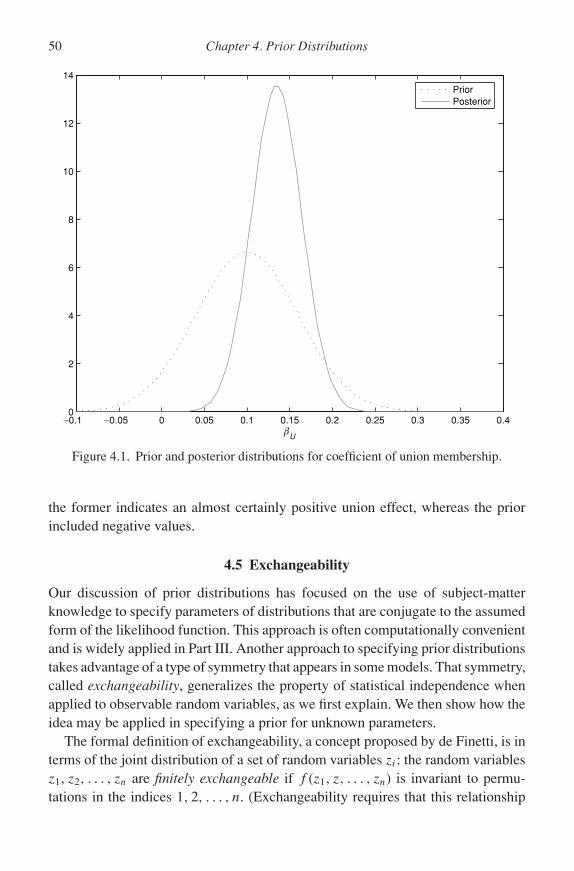
P1: KAE



−0.1 −0.05 0 0.05 0.1 0.15 0.2 0.25 0.3 0.35 0.40

2

4

6

8

10

12

14

βU

PriorPosterior

Figure 4.1. Prior and posterior distributions for coefficient of union membership.

the former indicates an almost certainly positive union effect, whereas the priorincluded negative values.

4.5 Exchangeability

Our discussion of prior distributions has focused on the use of subject-matterknowledge to specify parameters of distributions that are conjugate to the assumedform of the likelihood function. This approach is often computationally convenientand is widely applied in Part III. Another approach to specifying prior distributionstakes advantage of a type of symmetry that appears in some models. That symmetry,called exchangeability, generalizes the property of statistical independence whenapplied to observable random variables, as we first explain. We then show how theidea may be applied in specifying a prior for unknown parameters.

The formal definition of exchangeability, a concept proposed by de Finetti, is interms of the joint distribution of a set of random variables zi : the random variablesz1, z2, . . . , zn are finitely exchangeable if f (z1, z, . . . , zn) is invariant to permu-tations in the indices 1, 2, . . . , n. (Exchangeability requires that this relationship

P1: KAE


4.5 Exchangeability 51

hold for all n.) For example, if n = 3, the random variables z1, z2, and z3 areexchangeable if

f (z1, z2, z3) = f (z1, z3, z2)

= f (z2, z1, z3)

= f (z2, z3, z1)

= f (z3, z1, z2)

= f (z3, z2, z1).

Exchangeability generalizes the concept of independence: identically distributedand mutually independent random variables are exchangeable, but exchangeabilitydoes not imply independence. de Finetti and others have shown the power andimplications of this idea, but we use it in a more informal way.

Loosely speaking, a set of random variables is exchangeable if nothing other thanthe observations themselves distinguishes any of the zis from any of the others.For example, if a coin is tossed three times and two heads appear, the possibleoutcomes are HHT, HTH, or THH. If the only information we have is that threetosses resulted in two heads, then exchangeability requires that we assign the sameprobability to each of these three outcomes.

As an example of exchangeability applied to prior distributions, consider theproblem of heteroskedasticity in the linear regression model that arises when theassumption that Var(ui) is the same for all i is untenable. Suppose that the linearregression model is

f (yi |β, σ 2, λi) = N(x ′iβ, λ−1

i σ 2), (4.8)

and we further specify

β ∼ NK (β0, B0),

σ 2 ∼ IG(α0/2, δ0/2),

λi ∼ G(ν/2, ν/2).

(4.9)

A gamma prior distribution is appropriate for λi because it is a precision param-eter and therefore positive; the choice of parameters (ν/2, ν/2) is explained later.This assumption about the distribution of λi embodies exchangeability: each i isassociated with a particular λi , but the λi are drawn independently from the samegamma distribution. Knowing the value of i gives us no additional informationabout the value of λi . Although each observation has its own variance λ−1

i σ 2, allwe know about these variances is that they are drawn from the same distribution.This assumption about the variance can be contrasted with the assumption thatE(yi) = x ′

iβ, where the fact that each observation has its own covariate vector xi

P1: KAE



implies different expected values for each observation; that is, knowing the valueof i gives us covariate values xi that provide information about the mean level of yi .

While the heteroskedastic regression model is an example of specifying anexchangeable prior, it is of interest in its own right as an extension of the linearmodel. You should verify that the prior family is not conjugate and that the posteriordistribution is not of a standard form that permits analytic integration to obtain themarginal posterior distribution of β and σ 2. But the model has an interestingproperty that is exploited in Section 8.1.2. From our assumptions that ui |λi, σ

2 ∼N(0, λ−1

i σ 2) and λi ∼ G(ν/2, ν/2), we can write

f (ui, λi |σ 2) ∝ λ1/2i exp

[− λi

2σ 2u2

i

]λ

ν/2−1i exp

[−νλi

2

]∝ λ

(ν+1)/2−1i exp

[−λi(u2

i + νσ 2)

2σ 2

].

The marginal distribution f (ui |σ 2) is found by integrating (or marginalizing) overλi using the fact that λi |u2

i , σ2 has the distribution G[(ν + 1)/2, (u2

i + νσ 2)/2σ 2].Its normalizing constant is therefore proportional to (u2

i + νσ 2)−(ν+1)/2, from whichwe have

(u2i + νσ 2)−(ν+1)/2 ∝

(1 + u2

i

νσ 2

)−(ν+1)/2

,

the kernel of the Student-t distribution t(ν, 0, σ 2). We conclude that the aforemen-tioned assumption about the distribution of λi and the normality of ui |λi, σ

2 isequivalent to assuming that the ui |σ 2 have a t-distribution with ν degrees of free-dom. We can say that the distribution of ui is conditionally heteroskedastic becausethe variance of ui |λi, σ

2 = λ−1i σ 2, but the distribution of ui |σ 2 is homoskedastic.

4.6 Hierarchical Models

The models we have examined to this point contain two elements: a density functionfor the observed data conditioned on a vector of parameters and a prior distribu-tion for the parameters, in turn conditioned on a vector of hyperparameters. Ina hierarchical model, we add one or more additional levels, where the hyperpa-rameters themselves are given a prior distribution depending on another set ofhyperparameters; for example,

y ∼ f (y|θ ), (4.10)

θ ∼ π (θ |α0), (4.11)

α0 ∼ π (α0|α00), (4.12)

P1: KAE


4.7 Training Sample Priors 53

where α00 is specified. Other levels may be added, but this is rarely done. Beforeturning to an example, we make a few comments. First, α0 is not identified from thedata, because f (y|θ, α0) = f (y|θ ). Second, α0 can be eliminated from the problembecause

π (θ |α00) =∫

π (θ |α0)π (α0|α00) dα0.

Accordingly, α0 is neither identified nor necessary for analyzing the model; it isintroduced to facilitate computations or modeling.

As an example, consider the heteroskedastic linear model of Section 4.5. Thedistribution of λi is given a gamma distribution depending on the parameter ν,which turns out to be the degrees of freedom parameter of a t-distribution. Inthat formulation, ν is chosen by the researcher. In a hierarchical version of themodel, a prior distribution is placed on ν to reflect uncertainty over its value. Since0 < ν < ∞, any distribution confined to positive values could serve. Examplesare the gamma distribution, a distribution over a finite set of ν values, or thePoisson distribution truncated to ν > 0, where parameters would be chosen toreflect prior views. It is helpful to recall that the t-distribution approaches thenormal as ν increases, and the approximation is very close for the central part ofthe distribution when ν ≈ 30 or larger. We return to this model in Section 4.9.

4.7 Training Sample Priors

The device described in this section can be applied when the researcher has verylittle information on which to base a prior distribution, but has a large number ofobservations. The idea is to take advantage of the Bayesian updating discussedin Section 3.1.3. A portion of the sample is selected as the training sample. Itis combined with a relatively uninformative prior to yield a first-stage posteriordistribution. In turn, this the prior for the remainder of the sample. By a rela-tively uninformative prior, we mean a prior with a large variance and a mean ofzero.

A limiting case of an uninformative prior is a flat, improper prior for the regres-sion coefficients, π (β) ∝ c, and a flat, improper prior on log(σ ), π (σ ) ∝ 1/σ . Thesechoices lead to π (β|σ 2, y) = NK (β|β, σ 2(X′X)−1), where β = (X′X)−1X′y, theordinary least squares estimator, and π (σ 2|y) = IG(σ 2|(n − K)/2, S2/2], whereS2 = (y − Xβ)′(y − Xβ), the usual sum of squared residuals. Note that, in thiscase, the joint posterior distribution of (β, σ 2) is proper, despite the improper priordistribution.

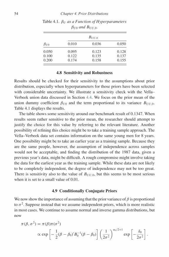
P1: KAE



Table 4.1. βU as a Function of HyperparametersβU0 and BUU,0.

BUU,0

βU0 0.010 0.036 0.050

0.050 0.095 0.123 0.1280.100 0.122 0.135 0.1370.200 0.174 0.158 0.155

4.8 Sensitivity and Robustness

Results should be checked for their sensitivity to the assumptions about priordistribution, especially when hyperparameters for those priors have been selectedwith considerable uncertainty. We illustrate a sensitivity check with the Vella–Verbeek union data discussed in Section 4.4. We focus on the prior mean of theunion dummy coefficient βU0 and the term proportional to its variance BUU,0.Table 4.1 displays the results.

The table shows some sensitivity around our benchmark result of 0.1347. Whenresults seem rather sensitive to the prior mean, the researcher should attempt tojustify the choice for this value by referring to the relevant literature. Anotherpossibility of refining this choice might be to take a training sample approach. TheVella–Verbeek data set contains information on the same young men for 8 years.One possibility might be to take an earlier year as a training sample. Because theyare the same people, however, the assumption of independence across sampleswould not be acceptable, and finding the distribution of the 1987 data, given aprevious year’s data, might be difficult. A rough compromise might involve takingthe data for the earliest year as the training sample. While these data are not likelyto be completely independent, the degree of independence may not be too great.There is sensitivity also to the value of BUU,0, but this seems to be most seriouswhen it is set to a small value of 0.01.

4.9 Conditionally Conjugate Priors

We now show the importance of assuming that the prior variance of β is proportionalto σ 2. Suppose instead that we assume independent priors, which is more realisticin most cases. We continue to assume normal and inverse gamma distributions, butnow

π (β, σ 2) = π (β)π (σ 2)

∝ exp

[− 1

2(β − β0)′B−1

0 (β − β0)

](1

2σ 2

)α0/2+1

exp

[− δ0

2σ 2

].

P1: KAE


4.9 Conditionally Conjugate Priors 55

To derive the posterior distribution, the prior is multiplied by the likelihood functionof (4.1). In this distribution, the parameters β and σ 2 are so interwoven thatwe cannot separate them into the product of two marginal distributions or of amarginal and conditional distribution. The distribution is not a standard form, andits normalizing constant is not known. Accordingly, even for one of the most basicmodels in applied statistics, the apparent slight change in the prior distributionresults in a model for which the desired marginal posterior distributions cannot bederived analytically.

But there is something interesting about this form: consider the conditionalposterior distributions π (β|σ 2, y) and π (σ 2|β, y). To derive the former, we consideronly the terms in the posterior that contain β. After some simplification, you shouldverify that

π (β|σ 2, y) ∝ exp

[− 1

2(β − β)′B−1

1 (β − β)

],

where

B1 = [σ−2X′X + B−1

0

]−1,

β = B1[σ−2X′y + B−1

0 β0].

We see that the conditional posterior distribution π (β|σ 2, y) is multivariate normalwith mean β and covariance matrix B1. When the conditional posterior distributionis in the same family as the prior, the prior is said to be conditionally conjugate orsemiconjugate.

It is important to be aware of how we found the conditional distribution becausethe method is used frequently later in the book. We first wrote down the expres-sion for the joint distribution of all parameters by the usual likelihood times priorformulation. We then picked out only the terms involving the parameters whoseconditional distribution we wish to determine. All terms that do not involve theseparameters are relegated to the proportionality constant. The remaining expres-sion, which contains the parameters of interest, is proportional to the conditionaldistribution of those parameters.

The idea is now applied to π (σ 2|β, y). To find this distribution, collect the termsin the joint posterior distribution that include σ 2 to obtain

π (σ 2|β, y) ∝(

1

σ 2

)α1/2+1

exp

[− δ1

2σ 2

],

where α1 = α0 + n and δ1 = δ0 + (y − Xβ)′(y − Xβ). We now see that the con-ditional posterior distribution of σ 2|β, y is IG(α1/2, δ1/2), another example of aconditionally conjugate prior distribution.

P1: KAE



As another example of conditionally conjugate priors, consider the heteroskedas-tic linear regression model specified in (4.8) and (4.9). We adopt a hierarchical ap-proach to that model by taking ν as an additional parameter. You should verify thatπ (β|σ 2, λ, y) is normal, π (σ 2|β, λ, ν, y) is inverted gamma, and π (λi |β, σ 2, ν, yi)is gamma, where λ = (λ1, . . . , λn). Note that, in each case, we have included inthe conditioning set only those variables that actually appear in the conditionaldistributions, rather than including all variables. To complete the analysis, a priorfor ν must be specified and an expression for its conditional distribution derived.For the prior, we assume that ν takes on J values, ν1, ν2, . . . , νJ , with probabilitiesp10, p20, . . . , pJ0, respectively. For example, the values of ν might be set to 5, 15,30, and 50 to allow a range of possibilities. At 50, the t-distribution is very closeto a normal distribution.

To derive the conditional posterior distribution of the probabilities, we write thejoint posterior distribution of all parameters as

π (β, σ 2, λ, ν|y) ∝ π (β)π (σ 2)n∏i

(λi

σ 2

)1/2

exp

[− λi

2σ 2(yi − x ′

iβ)2

]

× λν/2−1i

1

�(ν/2, ν/2)exp

[−νλi

2

] J∑j

pj01(ν = νj ),

(4.13)

where 1(A) is the indicator function that equals 1 if A is true and 0 otherwise. Notethat only the last four terms involve ν, and these involve no parameters other thanthe λi . This reflects the fact that ν is not identified by the data, although it dependson y through the λi . We can therefore write

π (νj |λ) ∝ pj0λνj /2−1i

1

�(νj/2, νj/2)exp

[−νj

∑i λi

2

], j = 1, . . . , J. (4.14)

The requirement that∑

j π (νj |λ) = 1 is enforced by dividing the individual termsin (4.14) by their sum.

While we have no interest in conditional distributions per se, the conditionaldistributions derived in this chapter can be exploited to find the marginal posteriordistributions of β and σ 2. How to do this is taken up in Part II and applied inPart III.

4.10 A Look Ahead

Methods of assigning prior distributions have been presented in this chapter alongwith the basics of the linear normal regression model. We have seen that the con-jugate prior distribution leads to a standard form for the joint posterior distributionof β and σ 2, leading to analytic results for the marginal posteriors of β and σ 2.

P1: KAE


4.11 Further Reading and References 57

In Exercise 4.3, you will find that the distributions of β and σ 2 can also be foundanalytically when the priors for β and σ 2 have the improper prior distributionsspecified there.

We have seen that when a conditionally conjugate prior is used, however, theresulting joint distribution does not have a standard form. The result is that themarginal distributions of β and σ 2 cannot be found analytically. This is a seriouslimitation because we are usually interested in the marginal posterior distributionof a few of the βks, and an inability to find these threatens the usefulness of theBayesian approach. If we cannot find marginal distributions for the most commonlyused model of econometrics and other fields, of what use is the approach?

There are several possible ways of dealing with this issue. One possibility isnumerical integration, a traditional method of evaluating integrals that do not haveanalytic solutions. But this method is useful only in low-dimensional problems.The union example discussed in Section 4.4 contains 32 regression parametersand one variance parameter. Numerical integration would not allow us to find themarginal distribution of the union regression coefficient.

Another approach utilizes the ability of computers to generate pseudorandomnumbers that are used to draw a sample from a distribution. A sample drawn thisway is called a “simulated sample” or a “simulation.” With a large sample from adistribution, it is possible to approximate the marginal distribution of the param-eters and of any continuous function of the parameters, including their moments.Simulation is an alternative to integration that can be used in high-dimensionalproblems, and simulation can be applied to standard and nonstandard distributions.The insight that simulation can help us learn about marginal distributions greatlyextends the reach of Bayesian inference, but to take advantage of this idea wemust learn how to simulate samples from whatever joint distribution we encounter.New approaches to simulation have made this possible. Part II of the book ex-plains general methods of simulating samples from both standard and nonstandarddistributions.


Section 4.2 See Garthwaite et al. (2005) for a summary of methods for elicitingprobability distributions. O’Hagan et al. (2006) is a book-length treatment of theelicitation of experts’ probability judgments. It explains and evaluates numerousmethods of elicitation and provides examples and many further references.

Section 4.5 See Bernardo and Smith (1994, chap. 4) and O’Hagan (1994, sec. 4.39–4.50, 6.36–6.38) for a detailed discussion of exchangeability, and Albert and Chib(1993b) and Geweke (1993) for further discussion of the heteroskedastic model.

P1: KAE



4.12 Exercises

4.1 Show that (4.6) can be rewritten as

δ1 = δ0 + (y − Xβ)′(y − Xβ) + (β0 − β)′[(X′X)−1 + B0]−1(β0 − β),

where β = (X′X)−1X′y, the ordinary least squares estimator of β for the frequentiststatistician in the normal linear regression model. (Hint: use (A.18).)

4.2 Let yi ∼ N (µ, 1) and take µ ∼ N (µ0, σ20 ) as the prior distribution, which becomes

improper as σ 20 → ∞. Derive π (µ|y), where y is a random sample of size n. Discuss

how the posterior distribution behaves as σ 20 → ∞.

4.3 This question refers to the expression for β in Section 4.3 and generalizes Exercise 4.2.Some authors suggest that weak prior information can be modeled as large priorvariances for β. For example, suppose that B0 is a matrix with large values on the maindiagonal and zeros elsewhere, and consider what happens to β as the variances go toinfinity. Interpret this result in terms of the weight assigned to the data and to the priorin determining the posterior distribution.

4.4 In Section 4.3, we showed that β|y has a multivariate t-distribution. Equations (A.12)–(A.14) give the marginal distribution and its moments for a subset of the parameters.Choose a data set that includes at least two covariates and find a 95% interval estimatefor β2.

4.5 Since the posterior distribution of (β, σ 2) in Section 4.3 is of known form, it is possibleto compute its marginal likelihood analytically. Start from the definition of the marginallikelihood:∫

f (y|β, σ 2)π (β, σ 2) dβ dσ 2

=∫ (

1

2πσ 2

)n/2

exp

[− 1

2σ 2(y − Xβ)′(y − Xβ)

](1

2πσ 2

)K/2

× 1

|B0|1/2exp

[− 1

2σ 2(β − β0)′B−1

0 (β − β0)

]× (δ0/2)α0/2

�(α0/2)

(1

σ 2

)α0/2+1

exp

[− δ0

2σ 2

]dβ dσ 2

=(

1

2π

)n/2 (δ0/2)α0/2

�(α0/2)

1

|B0|1/2

∫ {(1

2πσ 2

)K/2

× exp

[− 1

2σ 2(β − β)′B−1

1 (β − β)

]dβ

}{(1

σ 2

)α1/2+1

exp

[− δ1

2σ 2

]dσ 2

},

where we have used (4.5). Now integrate the first pair of curly braces as a multivariatenormal and the second as an inverted gamma to find this expression for the marginallikelihood: (

1

π

)n/2 |B1|1/2

|B0|1/2

�(α1/2)

�(α0/2)

δα0/20

δα1/21

.

P1: KAE


4.12 Exercises 59

4.6 Show that i.i.d. variables are exchangeable.4.7 Suppose that an urn contains R red balls and B blue balls and that three balls are

removed at random without replacement. Let Bi (respectively Ri) denote that a blue(respectively red) ball is removed at the ith draw, i = 1, 2, 3. Show that

P (R1, B2, B3) = P (B1, R2, B3) = P (B1, B2, R3),

but that P (R1) = P (R1|B2). Conclude that this distribution is finitely exchangeableand that the draws are not independent.

P1: KAE


60

P1: KAE


Part II

Simulation

61

P1: KAE


62

P1: KAE


Chapter 5

Classical Simulation

AS WE MENTIONED at the end of the previous chapter, simulation has greatlyexpanded the scope of Bayesian inference. In this chapter, we review methodsfor generating independent samples from probability distributions. The methodsdiscussed here form the basis for the newer methods discussed in Chapter 7 thatare capable of dealing with a greater variety of distributions but do not generateindependent samples.

All major statistics packages contain routines for generating random variablesfrom such standard distributions as those summarized in the appendix. The exam-ples presented here are intended to illustrate methods of generating samples. Wedo not claim that the algorithms are the best that can be designed, and we do notstudy the methods in great detail. Our goal for the chapter is to present the standardtechniques of simulation and explain the kinds of questions that simulated samplescan help answer.

Many of the applications discussed later can be regarded as attempts to approx-imate a quantity such as E[g(X)] where X ∼ f (X), but the necessary integral,∫

g(x)f (x) dx, cannot be computed analytically. This problem includes the com-putation of expected values (where g(X) = X) and other moments, as well asP (c1 ≤ X ≤ c2), for which we set g(X) = 1(c1 ≤ X ≤ c2).

5.1 Probability Integral Transformation Method

The most basic method of generating samples takes advantage of the ability ofcomputers to generate values that can be regarded as drawn independently from auniform distribution on (0,1), U (0, 1). For this discussion, we adopt the conventionthat a capital letter such as Z represents a random variable and the correspondingsmall letter z represents a particular value of that random variable.

Suppose we wish to draw a sample of values from a random variable that hasd.f. F (·), assumed to be nondecreasing. Consider the distribution of Z, which

63

P1: KAE


64 Chapter 5. Classical Simulation

is obtained by drawing U from U (0, 1) and setting Z = F−1(U ), which impliesU = F (Z):

P (Z ≤ z) = P (F (Z) ≤ F (z))

= P (U ≤ F (z))

= F (z),

where the first line relies on the fact that the d.f. is nondecreasing and the lastline uses the property of the uniform distribution that P (U ≤ u) = u. (If F (·) isconstant over one or more intervals of Z, it is evaluated at the smallest value of eachsuch interval.) We conclude that the random variable Z computed in this fashioncan be regarded as a draw from the d.f. F (·). This method, the probability integraltransformation (PIT) method, takes its name from the fact that U = F (Z) is calledthe probability integral transformation. It is also called the inverse d.f. method. Notethat a multivariate random variable cannot be simulated by this method, becauseits d.f. is not one-to-one and therefore not invertible.

In algorithmic form, we have the following.

Algorithm 5.1: Probability integral transform method

5.1 Draw u from U (0, 1).5.2 Return y = F−1(u) as a draw from f (y).

Implementing this method requires that the d.f. be known completely (i.e., itsnormalizing constant is known as well as its kernel) and that F−1(·) can be readilycomputed. Because accurate approximations to the inverse function have beencomputed for standard distributions and are available in many computer program,the latter requirement can be met even if the inverse function cannot be computedanalytically.

As our first example, suppose we desire to sample from U (a, b), a generalizationof the uniform distribution. Since

f (z) ={

1b−a

, if a ≤ z ≤ b,

0, otherwise,

we find F (z) = (z − a)/(b − a)1(a ≤ z ≤ b). If U ∼ U (0, 1), then U = (Z −a)/(b − a), and Z = a + (b − a)U is a draw from U (a, b).

As another example, suppose we wish to draw a sample from a random variablewith density function

y ∼ f (y) ={

38y

2, if 0 ≤ y ≤ 2,

0, otherwise.

P1: KAE


5.2 Method of Composition 65

We first find the d.f. for 0 ≤ y ≤ 2 by computing

F (y) = 3

8

∫ y

0t2 dt = 1

8y3.

The next step is to draw a value U from U (0, 1) and set U = (1/8)Y 3. We thensolve to find Y = 2U 1/3, which is a draw from f (Y ).

An important application of this method is to the problem of sampling from atruncated distribution. Suppose that X has d.f. F (X) and that we wish to generatevalues of X restricted to c1 ≤ X ≤ c2. The distribution of the truncated values is[F (X) − F (c1)]/[F (c2) − F (c1)] for c1 ≤ X ≤ c2. Following our usual procedure,we generate U ∼ U (0, 1) and set

U = F (X) − F (c1)

F (c2) − F (c1),

which implies that

X = F−1(F (c1) + U [F (c2) − F (c1)]) (5.1)

is a drawing from the truncated distribution. This method is routinely used tosample from univariate truncated normal or Student-t densities because accurateapproximations to the inverse d.f.s are available and included in statistics packages.

5.2 Method of Composition

The method of composition uses the relationship

f (x) =∫

g(x|y)h(y) dy,

where f , g, and h are densities. The method is useful when we know how to sampley from h(y) and x from g(x|y). By drawing a y from h(y) and then an x fromg(x|y), the value of x is a drawing from f (x).

We have seen an example of this idea in Section 4.5 in connection with theheteroskedastic linear regression model. It was shown that if ui |λi ∼ N(0, λ−1

i σ 2),λi ∼ G(ν/2, ν/2), and

f (ui |σ 2) =∫

g(ui |λi, σ2)h(λi) dλi,

where g(ui |λi, σ2) is the density function of N(ui |0, λ−1

i σ 2) and h(λi) is the densityfunction of G(λi |ν/2, ν/2), then f (ui |σ 2) is the density function of t(ν, 0, σ 2). Thisresult shows that we can simulate draws from a t-distribution with ν degrees offreedom if we know how to simulate draws from a gamma distribution and from anormal distribution: draw a value of λi from the gamma distribution and then draw

P1: KAE



a value of ui from the normal distribution conditional on the value of λi . This resultgeneralizes to simulation from t-distributions with nonzero means.

The method of composition can be thought of as a mixture distribution, where thedensity of interest can be written as the marginal distribution of a joint distribution,

f (x) =∫

g(x, y) dy.

In this form, g(·, ·) is not explicitly written as the product of a conditional and amarginal density. The mixture distribution idea can be used when it is convenientto sample a joint distribution. The expression implies that the values of x are asample from its marginal distribution when a sample (x, y) is generated from theirjoint distribution.

It is sometimes possible to write a p.d.f. in the form of a finite mixture distribution,

f (x) =k∑i

Pifi(x),

where∑

Pi = 1 and each fi(x) is a p.d.f. If it is known how to sample from eachof the fi(·), a sample from f (·) can be obtained by choosing i with probability Pi

and then generating a value from fi . See Exercise 5.3 for an example.

5.3 Accept–Reject Algorithm

The accept–reject (AR) algorithm can be used to simulate values from a densityfunction f (·) if it is possible to simulate values from a density g(·) and if a numberc can be found such that f (Y ) ≤ cg(Y ), c ≥ 1, for all Y in the support of f (·). Thedensity f (Y ) to be sampled is called the target density, the distribution g(y) thatis simulated is called the majorizing, instrumental, or proposal density, and cg(·)is called the majorizing function or dominating density. The target density must bedominated over the entire support of Y , which is often difficult to achieve in themultivariate case.

The AR algorithm proceeds as follows.

Algorithm 5.2: Accept–reject method

5.1 Generate a value y from g(·).5.2 Draw a value u from U (0, 1).5.3 Return y as a draw from f (·) if u ≤ f (y)/cg(y). If not, reject it and return to step 1.

(The effect of this step is to accept y with probability f (y)/cg(y).)

The procedure is continued until the desired number of draws is obtained.

P1: KAE


5.3 Accept–Reject Algorithm 67

Here is a proof to show the method works. Consider the distribution of theaccepted values of y, h[y|u ≤ f (y)/cg(y)]. By Bayes theorem and the property ofthe uniform distribution that P (u ≤ t) = t , 0 ≤ t ≤ 1, we have

h[y|u ≤ f (y)/cg(y)] = P [u ≤ f (y)/cg(y)|y]g(y)∫P [u ≤ f (y)/cg(y)|y]g(y) dy

= [f (y)/cg(y)]g(y)

(1/c)∫

f (y) dy

= f (y).

We have shown that the distribution of the accepted values has the distributionof the random variable from which we wish to sample. Note that∫

P (u ≤ f (y)/cg(y)|y)g(y) dy = 1/c

is the probability that a generated value of y is accepted. This implies that weshould choose c as small as possible to maximize the probability of acceptancebecause rejected values use computer time without adding to the sample.

Before proceeding with examples, we point out an interesting feature of the ARalgorithm that is useful when the normalizing constant of f (·) is unknown; that is,f (·) = kr(·) and r(·) is known but k is not. Let c be chosen so that r(y) ≤ cg(y).You can verify that if a value of y generated from g(y) is accepted with probabilityr(y)/cg(y), the accepted values of y are a sample from f (y). This method cantherefore be used even if the normalizing constant of the target distribution isunknown; in this case, it is no longer required that c ≥ 1.

As our first example, consider the problem of sampling from Beta(3, 3) withU (0, 1) as the proposal density. The maximum of the target density occurs at y =1/2, where the density function equals 1.8750. Accordingly, we set c = 1.8750, andthe probability of accepting a draw is 1/c = 0.5333. You can see from Figure 5.1why this proposal density is not a particularly good choice. It generates valuesuniformly along the horizontal axis, but the target density is far from uniform.Since values near zero and one are oversampled by the proposal density, theyare accepted with low probability to compensate for the oversampling. The figureshows that a value of 0.15 generated by the proposal is accepted with probability0.4877/1.875 = 0.2601.

The algorithm to implement this procedure may be summarized as follows.

Algorithm 5.3: Beta distribution

5.1 Draw u1 and u2 from U (0, 1).5.2 If

u2 ≤ Beta(3, 3)−1u21(1 − u1)2

1.8750,

return y = u1 as a draw from the target distribution. Otherwise reject it and return to 1.

P1: KAE



0 0.1 0.2 0.3 0.4 0.5 0.6 0.7 0.8 0.9 10

0.4877

1.875

f(y)=Beta(3,3)

cg(y)=1.875 U(0,1)

Figure 5.1. Target and proposal density to sample from Beta(3, 3).

As a second example, let the target density be N(0, 1) and the proposal densitybe the Laplace distribution, g(y) = (1/2) e−|y|. Since both of these are symmetricabout zero, we first sample from the exponential distribution, e−y , y > 0, andaccept or reject the value with the AR algorithm. If the proposal is accepted, itis assigned a positive value with probability one half and a negative value withprobability one half. This algorithm can be used for general normal distributions:if Y ∼ N(0, 1), then X = µ + σY ∼ N(µ, σ 2). To determine c verify that themaximum of (

√2π)−1 e−y2/2/e−y occurs at y = 1, implying that c = √

e/2π andthat the probability of acceptance is 1/c = 0.6577. Figure 5.2 displays the targetand proposal densities. In algorithmic form, we have the following.

Algorithm 5.4: Normal distribution

5.1 Generate u1, u2, and u3 from U (0, 1).5.2 Sample from the exponential distribution g(x) = e−x by the method of Section 5.1:

from g(x) = e−x , verify that G(x) = 1 − e−x . Accordingly, write u1 = 1 − e−x orx = −log(1 − u1), which is equivalent to x = −log(u1) since u1 and 1 − u1 have thesame distribution.

P1: KAE


5.3 Accept–Reject Algorithm 69

0 0.5 1 1.5 2 2.5 3 3.5 4 4.5 50

0.1

0.2

0.3

0.4

0.5

0.6

0.7

y

f(y)

cg(y)

Figure 5.2. Target and proposal density to sample from N (0, 1).

5.3 If

u2 ≤ 1√2π

e−x2/2

/ce−x

= 1√2π

e−x2/2

/√e

2πe−x (5.2)

= ex−x2/2−1/2,

return y = x if u3 ≤ 1/2 and y = −x if u3 > 1/2. If (5.2) is not satisfied, reject x andreturn to step 1.

The AR method may appear to be similar to the Metropolis–Hastings (MH)algorithm, discussed in the next chapter, because both involve a rejection step,but there are important differences. First, the MH method is more general thanthe AR method, in the sense that it can be employed to sample from a greatervariety of distributions. Second, the MH method generates correlated, rather thanindependent, samples. Independent samples are, in general, preferred to positivelycorrelated samples because they have a smaller variance and therefore provide more

P1: KAE



information from a given sample size. Although negatively correlated samples havean even smaller variance than do independent samples, the MH method tends toproduce positively correlated samples. Moreover, there are no known methods thatare sure to generate independent or negatively correlated samples.

5.4 Importance Sampling

Suppose that X ∼ f (X) and we wish to estimate

E[g(X)] =∫

g(x)f (x) dx,

but the integral is not computable analytically and the method of composition is notavailable, because we cannot sample from f (x). The importance sampling method,a type of Monte Carlo integration, works as follows. Let h(X) be a distributionfrom which we know how to simulate and consider the integral

E[g(X)] =∫

g(x)f (x)

h(x)h(x) dx.

This integral can be approximated by drawing a sample of G values from h(X),with values X(g), and computing

E[g(X)] ≈ 1

G

∑g(X(g))

f (X(g))

h(X(g)).

This expression can be regarded as a weighted average of the g(X(g)), where theimportance weights are f (X(g))/h(X(g)).

The main issue in implementation of importance sampling is the choice ofh(·). To find a suitable distribution we examine the variance of the estimate. SinceVar(g) = E(g2) − E(g)2 and the latter converges to E[g(X)]2, we may concentrateon

E(g2) =∫

g(x)2

(f (x)

h(x)

)2

h(x) dx.

This integral is large when f (x)/h(x) is large, a situation that tends to occur whenthe tail values of h(·) are very small compared to the tail values of f (·). Since thenormal distribution tends to zero very quickly, it is often not a good choice for h(·).In general, Var(g) is small when f (·)/h(·) does not vary greatly.

As an example of importance sampling, we approximate E[(1 + x2)−1], wherex ∼ exp(1), truncated to [0, 1]; that is, we approximate the integral

1

1 − e−1

∫ 1

0

1

1 + x2e−x dx.

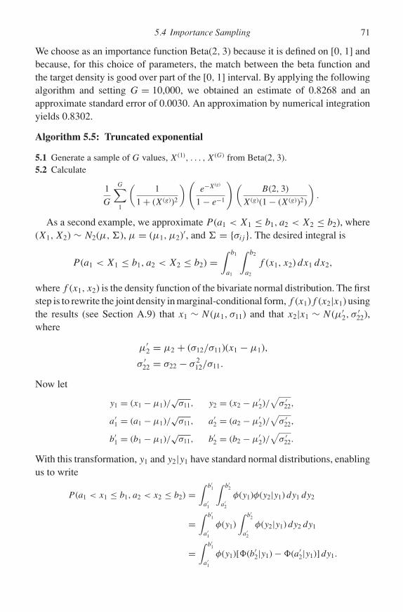
P1: KAE


5.4 Importance Sampling 71

We choose as an importance function Beta(2, 3) because it is defined on [0, 1] andbecause, for this choice of parameters, the match between the beta function andthe target density is good over part of the [0, 1] interval. By applying the followingalgorithm and setting G = 10,000, we obtained an estimate of 0.8268 and anapproximate standard error of 0.0030. An approximation by numerical integrationyields 0.8302.

Algorithm 5.5: Truncated exponential

5.1 Generate a sample of G values, X(1), . . . , X(G) from Beta(2, 3).5.2 Calculate

1

G

G∑1

(1

1 + (X(g))2

)(e−X(g)

1 − e−1

)(B(2, 3)

X(g)(1 − (X(g))2)

).

As a second example, we approximate P (a1 < X1 ≤ b1, a2 < X2 ≤ b2), where(X1, X2) ∼ N2(µ, ), µ = (µ1, µ2)′, and = {σij }. The desired integral is

P (a1 < X1 ≤ b1, a2 < X2 ≤ b2) =∫ b1

a1

∫ b2

a2

f (x1, x2) dx1 dx2,

where f (x1, x2) is the density function of the bivariate normal distribution. The firststep is to rewrite the joint density in marginal-conditional form, f (x1)f (x2|x1) usingthe results (see Section A.9) that x1 ∼ N(µ1, σ11) and that x2|x1 ∼ N(µ′

2, σ′22),

where

µ′2 = µ2 + (σ12/σ11)(x1 − µ1),

σ ′22 = σ22 − σ 2

12/σ11.

Now let

y1 = (x1 − µ1)/√

σ11, y2 = (x2 − µ′2)/√

σ ′22,

a′1 = (a1 − µ1)/

√σ11, a′

2 = (a2 − µ′2)/√

σ ′22,

b′1 = (b1 − µ1)/

√σ11, b′

2 = (b2 − µ′2)/√

σ ′22.

With this transformation, y1 and y2|y1 have standard normal distributions, enablingus to write

P (a1 < x1 ≤ b1, a2 < x2 ≤ b2) =∫ b′

1

a′1

∫ b′2

a′2

φ(y1)φ(y2|y1) dy1 dy2

=∫ b′

1

a′1

φ(y1)∫ b′

2

a′2

φ(y2|y1) dy2 dy1

=∫ b′

1

a′1

φ(y1)[�(b′2|y1) − �(a′

2|y1)] dy1.

P1: KAE



The algorithm is now implemented by choosing the standard normal distributiontruncated to (a′

1, b′1) as the importance distribution; that is, draw Y

(g)1 from the

truncated standard normal using (5.1). With this choice for the importance function,we have

P (a1 < X1 ≤ b1, a2 < X2 ≤ b2)

≈ 1

G

∑[�(b′

2

∣∣Y (g)1

)− �(a′

2

∣∣Y (g)1

)][�(b′

1

)− �(a′

1

)]. (5.3)

5.5 Multivariate Simulation

We have seen an example of simulating from a multivariate distribution in theprevious section. In general, as might be expected, sampling from multivariatedistributions is more difficult than is sampling from univariate distributions.

The multivariate distribution most studied is the multivariate normal Np(µ, ).Independent samples generated from the univariate normal can be transformed intosamples from the multivariate normal. To draw a sample from Np(µ, ), first drawp values from N(0, 1) and place them in a p × 1 vector Z, so that Z ∼ Np(0, Ip).Next, write = C ′C, where C is a p × p upper-triangular Cholesky matrix. (TheCholesky matrix for a given is computed in many statistical packages, althoughsome provide a lower-triangular version.) Finally, compute X = µ + C ′Z. You cannow verify that X ∼ Np(µ, ).

Although algorithms to simulate from all the multivariate distributions discussedin the appendix are available in the major statistical packages, designing an algo-rithm to generate independent samples from a nonstandard distribution can beextremely challenging. The AR and importance sampling methods can be usedin principle, but their implementation may be difficult: the AR requires findinga dominating density over the whole support, and importance sampling requiresfinding a distribution with sufficiently heavy tails.

5.6 Using Simulated Output

A sample of size G generated from f (Y ), where the individual values are denotedby Y (g), g = 1, . . . , G, can be used to investigate properties of the distributionin many ways. For example, we can graph the histogram or a kernel-smoothedversion of the histogram to see the shape of the distribution; we can approximatethe distribution of any continuous function of the sample, including moments; andwe can approximate the quantiles of a distribution.

As an example, suppose we are interested in the distribution of Z = XY , whereX ∼ Beta(3, 3) and Y ∼ Beta(5, 3), independently. A search turned up no analyticsolution to the distribution of Z, so we proceed by generating samples from X and

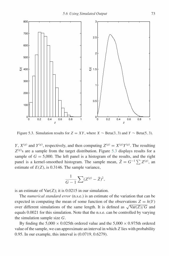
P1: KAE


5.6 Using Simulated Output 73

0 0.2 0.4 0.6 0.8 10

100

200

300

400

500

600

700

800

z

f(z)

0 0.2 0.4 0.6 0.8 10

0.5

1

1.5

2

2.5

3

z

f(z)

Figure 5.3. Simulation results for Z = XY , where X ∼ Beta(3, 3) and Y ∼ Beta(5, 3).

Y , X(g) and Y (g), respectively, and then computing Z(g) = X(g)Y (g). The resultingZ(g)s are a sample from the target distribution. Figure 5.3 displays results for asample of G = 5,000. The left panel is a histogram of the results, and the rightpanel is a kernel-smoothed histogram. The sample mean, Z = G−1∑Z(g), anestimate of E(Z), is 0.3146. The sample variance,

1

G − 1

∑(Z(g) − Z)2,

is an estimate of Var(Z); it is 0.0215 in our simulation.The numerical standard error (n.s.e.) is an estimate of the variation that can be

expected in computing the mean of some function of the observations Z = h(Y )over different simulations of the same length. It is defined as

√Var(Z)/G and

equals 0.0021 for this simulation. Note that the n.s.e. can be controlled by varyingthe simulation sample size G.

By finding the 5,000 × 0.025th ordered value and the 5,000 × 0.975th orderedvalue of the sample, we can approximate an interval in which Z lies with probability0.95. In our example, this interval is (0.0719, 0.6279).

P1: KAE



A major use of simulated data is to study the marginal distribution of a variable.This is especially important for Bayesian inference. Suppose that the target distribu-tion is the posterior distribution π (θ |y) of a vector of parameters θ = (θ1, . . . , θd)and that we have generated a sample of size G from that distribution, arrayed asfollows:

θ(1)1 θ

(1)2 · · · θ

(1)d

θ(2)1 θ

(1)2 · · · θ

(2)d

......

......

θ(G)1 θ

(G)2 · · · θ

(G)d .

Each row is a draw from the joint posterior distribution, but what can be said aboutthe columns? Let us focus on the first column as an example. From the definitionof the marginal distribution,

π (θ1|y) =∫

π (θ |y) dθ2· · · dθd ,

we see that the values in the first column are a draw from π (θ1|y), the values inthe second column are draws from π (θ2|y), and so on. This is a remarkable result:drawing a sample from the joint distribution provides samples from each of themarginal distributions without computing any integrals. This result extends to themethods presented in the next chapter with the difference that the samples fromeach of the marginal distributions are not independent, because the draws from thejoint distribution are not independent.


Section 5 The increasing importance of learning about simulation is high-lighted by noting that the only new chapter in the third edition of a widelyused statistics text, DeGroot and Schervish (2002), is about simulation. Use-ful references are Rubinstein (1981), Devroye (1986), Ripley (1987), Robertand Casella (2004), and Gentle (2003). The Devroye book is freely availableat cgm.cs.mcgill.ca/∼luc/rnbookindex.html.

Section 5.2 See Robert and Casella (2004, p. 45) for the mixture distribution idea.

Section 5.3 The example in which a normal is approximated by a Laplace is basedon an exercise in DeGroot and Schervish (2002, p. 726, ex. 6).

Section 5.4 Importance sampling is discussed in several of the books cited before.An important reference to the subject in the econometrics literature is Geweke(1989). The truncated exponential algorithm is based on an example in DeGroot

P1: KAE


5.8 Exercises 75

and Schervish (2002, pp. 728–729), where different importance functions are used.The GHK algorithm, which generalizes the bivariate normal example, is namedfor J. Geweke, V. Hajivassiliou, and M. Keane. It is described in Greene (2003,pp. 932–933) and in Train (2003, sec. 5.6.3)

5.8 Exercises

5.1 Use the probability integral transformation method to simulate from the distribution

f (x) ={

2a2 x, if 0 ≤ x ≤ a,

0, otherwise,

where a > 0. Set a value for a, simulate various sample sizes, and compare results tothe true distribution.

5.2 Use the probability integral transformation method to simulate 500 values from thelogistic distribution,

f (x) = e−x

(1 + e−x)2, −∞ < x < ∞.

Compare your simulated values to the true distribution. Explore how the simulationimproves with larger sample sizes. Generalize your result to the general form of thedistribution,

f (x) = exp[−(x − α)/β]

β(1 + exp[−(x − α)/β])2, −∞ < x < ∞, α, β > 0.

5.3 Generate samples from the distribution

f (x) = 2

3e−2x + 2 e−3x

using the finite mixture approach. Hint: Note that the p.d.f. can be written as

f (x) = 1

3(2 e−2x) + 2

3(3 e−3x).

5.4 Draw 500 observations from Beta(3, 3) using algorithm 5.3. Compute the mean andvariance of the sample and compare them to the true values.

5.5 Draw 500 observations from N (2, 4) using Algorithm 5.4. Compute the mean andvariance of the sample and compare them to the true values. Overlay a histogram ofthe sample values on a graph of the true distribution and discuss how well the sampleapproximates the true distribution.

5.6 Verify Equation (5.3).5.7 Use importance sampling to compute P (0.2 < x1 ≤ 2,−1 < x2 ≤ 5), where

(x1, x2) ∼ N2(µ,), µ = (1,−0.5)′, and

=(

2 11 3

).

P1: KAE


Chapter 6

Basics of Markov Chains

WE HAVE SEEN in the previous chapter that there exist methods to generateindependent observations from the standard probability distributions, includingthose described in the appendix. But we still have the problem of what to do whenfaced with a nonstandard distribution such as the posterior distribution of parame-ters of the conditionally conjugate linear regression model. Although the methodsdescribed before can, in principle, deal with nonstandard distributions, doing sopresents major practical difficulties. In particular, they are not easy to implement inthe multivariate case, and finding a suitable importance function for the importancesampling algorithm or a majorizing density for the AR algorithm may require a verylarge investment of time whenever a new nonstandard distribution is encountered.

These considerations impeded the progress of Bayesian statistics until the devel-opment of Markov chain Monte Carlo (MCMC) simulation, a method that becameknown and available to statisticians in the early 1990s. MCMC methods haveproved to be extremely effective and have greatly increased the scope of Bayesianmethods. Although a disadvantage of this family of methods is that it does notprovide independent samples, it has the great advantage of flexibility: it can beimplemented for a great variety of distributions without having to undertake anintensive analysis of the special features of the distribution. We note, however, thatan analysis of the distribution may shed light on the best algorithm to use whenmore than one is available.

Since these methods rely on Markov chains, a type of stochastic process, thischapter presents some basic concepts of the theory, and the next chapter utilizesthese concepts to explain MCMC methods.

6.1 Finite State Spaces

Consider a stochastic process indexed by t , Xt, that takes values in the finite setS = {1, 2, . . . , s}. The index t is interpreted as time or iterate. For any pair of

76

P1: KAE


6.1 Finite State Spaces 77

integers i, j ∈ S, pij is defined as the probability that Xt+1 = j given that Xt = i,

that is,

pij = P (Xt+1 = j |Xt = i), i, j ∈ S. (6.1)

The pij are transition probabilities. The assumption that the probability distributionat time t + 1 depends only on the state of the system at t is called the Markovproperty, and the resulting stochastic process is a Markov process. A Markovprocess is more general than is an independent process, but does not include allstochastic processes. We further assume, implicit in the notation, that the pij donot depend on t. This type of stochastic process is called a homogeneous Markovchain. These simple definitions and assumptions generate a powerful and elegantmathematical theory.

Since the pij are probabilities, we have pij ≥ 0, and since the process remainsin S,

s∑j=1

pij = 1.

It is convenient to define the s × s transition matrix P = {pij }. The ith row of P ,(pi1, . . . , pis), specifies the distribution of the process at t + 1, given that it is instate i at t .

For example, the transition matrix,

P =(

0.750 0.250

0.125 0.875

), (6.2)

specifies that the process remains in state 1 with probability 0.750 and moves tostate 2 with probability 0.250 if it starts in state 1. And, if it starts in state 2, it movesto state 1 with probability 0.125 and remains in state 2 with probability 0.875.

Now consider the distribution of the state at t + 2, given that it is in i at t . Thisdistribution is denoted by p

(2)ij and can be computed as follows: to go from state i

to state j in two steps, the process goes from i at t to any other state k at time t + 1and then from k to j at t + 2. This transition occurs with probability

p(2)ij =

∑k

pikpkj . (6.3)

You can verify that the matrix of the p(2)ij is given by PP ≡ P 2. Having done so, you

can show by induction that the values of p(n)ij are the ij th entries in the matrix P n,

where n is any integer. It is convenient to define p(0)ij as 1 if i = j and 0 otherwise.

We will be mostly concerned with what happens to p(n)ij as n becomes large. Before

doing so, we present an example and a few definitions.

P1: KAE


78 Chapter 6. Basics of Markov Chains

A simple example is that of completely random motion or independence: let allrows of P be identical, that is, pij = pj for all i. In this case, the probability ofmoving from state i to state j depends only on j . An independent coin tossingexperiment is an example. Let heads be state 1 and tails be state 2. Let p1 = 2/3and p2 = 1/3. Verify that each row of the transition matrix is the same.

If p(n)ij > 0 for some n ≥ 1, we say j is accessible from i and write i → j.

If i → j and j → i, we say i and j communicate, and write i ↔ j. It can beshown that the communication relationship between states defines an equivalencerelationship; that is, i ↔ i (reflexivity); i ↔ j ⇐⇒ j ↔ i (symmetry); and i ↔j and j ↔ k ⇒ i ↔ k (transitivity).

This equivalence relationship places the states into equivalence classes withinwhich the states communicate. A very important idea in the theory can now bedefined: a Markov process is irreducible if there is just one equivalence class.What this means is that starting from state i, the process can reach any other statewith positive probability. Suppose, for example, P takes the form

PR =(

P1 00 P2

), (6.4)

where P1 and P2 are m × m. Then it should be easy to see that if the process startsin any of the first m states, it will never leave them. And, of course, if it starts inone of the states m + 1, . . . , 2m, it will never leave them either. The process PR isnot irreducible, and the state at which the process begins has a very large effect onits subsequent path.

Another important property of a chain is periodicity. Consider a transition matrixof the form

PP =(

0 P1

P2 0

), (6.5)

where P1 and P2 are m × m. If at t = 1, the process is in one of the first m states,it must go to one of the second m at t = 2, whereupon it must return to the first m

states at t = 3, and so on. Positive probabilities of returning to a state in either ofthe two subsets exist only at even values of n. This is described by saying the periodis of the chain is 2. If the period is 1 for all states, the chain is said to be aperiodic.More formally, if i → i, then the period of i is the greatest common divisor ofthe integers in the set A = {n ≥ 1 : p

(n)ii > 0}. In words, if di is the period of i,

then p(n)ii = 0 whenever n is not a multiple of di , and di is the largest integer with

this property. Note that a chain is aperiodic if p(n)ii > 0 for all i and for sufficiently

large n.

P1: KAE


6.1 Finite State Spaces 79

MCMC methods are based on the next definition. The probability distributionπ = (π1, . . . , πs)′ is an invariant distribution for P if π ′ = π ′P , or

πj =∑

i

πipij , j = 1, . . . , s. (6.6)

The right-hand side of this equation is the probability that the process is in state j

at any t marginalized over the states at t − 1; it can be interpreted as the probabilityof starting the process at state i with probability πi and then moving to state j withprobability pij . The fact that the resulting value is πj is what makes π an invariantdistribution: if the states are chosen according to π , the probability is πj that thesystem is in state j at any time. Note that π ′ is a characteristic vector of P with acharacteristic root equal to 1.

For an example of an invariant distribution, consider the transition matrix ofEquation (6.2). From π ′P = π ′, we have

(π1, π2)

(0.750 0.2500.125 0.875

)= (π1, π2),

or

0.750π1 + 0.125π2 = π1,

and, since π2 = 1 − π1,

π1 = 0.750π1 + 0.125(1 − π1),

which implies π = (1/3, 2/3). This example is generalized in Exercise 6.2.An important topic in Markov chain theory is the existence and uniqueness of

invariant distributions. We can see immediately that irreducibility is a necessarycondition for P to have a unique invariant distribution: in PR mentioned earlier,let π1 satisfy π ′

1P1 = π ′1 and π2 satisfy π ′

2P2 = π ′2. Then it is easy to verify that

π = (wπ1, (1 − w)π2), 0 ≤ w ≤ 1, is an invariant distribution for P , which showsthat the invariant distribution is not unique.

A special case of an irreducible and aperiodic Markov chain is one in which allpij > 0. For these, we have the following theorem.

Theorem 6.1 Suppose S is finite and pij > 0 for all i, j. Then there exists aunique probability distribution πj , j ∈ S, such that

∑i πipij = πj for all j ∈ S.

Moreover,

|p(n)ij − πj | ≤ rn, (6.7)

where 0 < r < 1, for all i, j and n ≥ 1.

A proof may be found in Bhattacharya and Waymire (1990, p. 126).

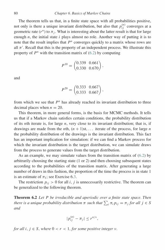
P1: KAE



The theorem tells us that, in a finite state space with all probabilities positive,not only is there a unique invariant distribution, but also that p

(n)ij converges at a

geometric rate (rn) to πj . What is interesting about the latter result is that for largeenough n, the initial state i plays almost no role. Another way of putting it is tonote that the result implies that P n converges quickly to a matrix whose rows areall π ′. Recall that this is the property of an independent process. We illustrate thisproperty of P n with the transition matrix of (6.2) by computing

P 10 =(

0.339 0.6610.330 0.670

),

and

P 20 =(

0.333 0.6670.333 0.667

),

from which we see that P n has already reached its invariant distribution to threedecimal places when n = 20.

This theorem, in more general forms, is the basis for MCMC methods. It tellsus that if a Markov chain satisfies certain conditions, the probability distributionof its nth iterate is, for large n, very close to its invariant distribution; that is, ifdrawings are made from the nth, (n + 1)st, . . . iterate of the process, for large n

the probability distribution of the drawings is the invariant distribution. This facthas an important implication for simulation: if we can find a Markov process forwhich the invariant distribution is the target distribution, we can simulate drawsfrom the process to generate values from the target distribution.

As an example, we may simulate values from the transition matrix of (6.2) byarbitrarily choosing the starting state (1 or 2) and then choosing subsequent statesaccording to the probabilities of the transition matrix. After generating a largenumber of draws in this fashion, the proportion of the time the process is in state 1is an estimate of π1; see Exercise 6.3.

The restriction pij > 0 for all i, j is unnecessarily restrictive. The theorem canbe generalized to the following theorem.

Theorem 6.2 Let P be irreducible and aperiodic over a finite state space. Thenthere is a unique probability distribution π such that

∑i πipij = πj for all j ∈ S

and

|p(n)ij − πj | ≤ rn/ν,

for all i, j ∈ S, where 0 < r < 1, for some positive integer ν.

P1: KAE


6.2 Countable State Spaces 81

A proof may be found in Bhattacharya and Waymire (1990, p. 128). The proofinvolves making estimates of the difference between successive values of |p(n)

ij −πj | and showing these go to zero with n.

Rather than prove the theorem, let us see what happens when the assumptionsare violated. First consider the reducible transition matrix PR. We have alreadynoted that it does not have a unique invariant distribution. Since

P nR =

(P n

1 00 P n

2

),

its nth iterate does not have the same probability distribution in each of its rowsand does not converge to anything useful for MCMC purposes. Next consider theirreducible but periodic matrix PP : we have

P 2P =

(P1P2 0

0 P2P1

),

and

P 3P =

(0 P1P2P1

P2P1P2 0

).

Since this alternating pattern continues for every iterate, P nP does not converge to

a matrix with identical rows. Thus, irreducibility and aperiodicity are necessaryconditions for the theorem.

Although Theorem 6.2 states that irreducibility and aperiodicity are sufficientto yield a result that justifies the MCMC method for finite state spaces, we need toconsider more general state spaces because most applications involve continuousdistributions. Before turning to these and the additional complications they bring,we briefly examine Markov chains with a countable number of states.

6.2 Countable State Spaces

An example of a countable state space is the simple random walk. In this process,S = {0, ±1, ±2, . . .}, and the transition probabilities are

pij =

p, if j = i + 1,

q, if j = i − 1,

0, otherwise,

where 0 < p < 1 and q = 1 − p. The possible states are all positive and negativeintegers, a countable space.

Irreducibility and aperiodicity no longer imply the existence of a unique invariantdistribution when S is countable but not finite. Another concept, recurrence, must

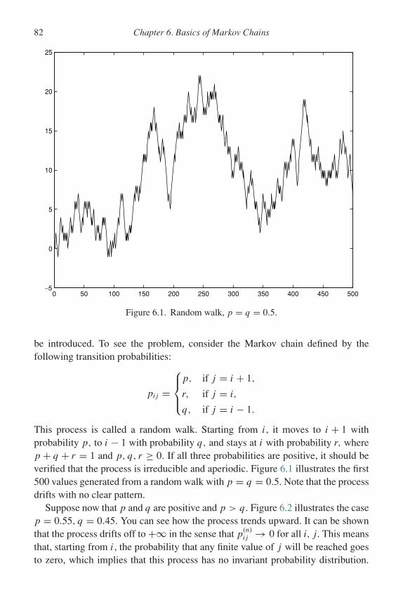
P1: KAE



0 50 100 150 200 250 300 350 400 450 500−5

0

5

10

15

20

25

Figure 6.1. Random walk, p = q = 0.5.

be introduced. To see the problem, consider the Markov chain defined by thefollowing transition probabilities:

pij =

p, if j = i + 1,

r, if j = i,

q, if j = i − 1.

This process is called a random walk. Starting from i, it moves to i + 1 withprobability p, to i − 1 with probability q, and stays at i with probability r, wherep + q + r = 1 and p, q, r ≥ 0. If all three probabilities are positive, it should beverified that the process is irreducible and aperiodic. Figure 6.1 illustrates the first500 values generated from a random walk with p = q = 0.5. Note that the processdrifts with no clear pattern.

Suppose now that p and q are positive and p > q. Figure 6.2 illustrates the casep = 0.55, q = 0.45. You can see how the process trends upward. It can be shownthat the process drifts off to +∞ in the sense that p

(n)ij → 0 for all i, j. This means

that, starting from i, the probability that any finite value of j will be reached goesto zero, which implies that this process has no invariant probability distribution.

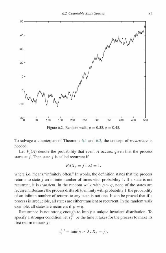
P1: KAE


6.2 Countable State Spaces 83

0 50 100 150 200 250 300 350 400 450 500−20

−10

0

10

20

30

40

50

Figure 6.2. Random walk, p = 0.55, q = 0.45.

To salvage a counterpart of Theorems 6.1 and 6.2, the concept of recurrence isneeded.

Let Pj (A) denote the probability that event A occurs, given that the processstarts at j . Then state j is called recurrent if

Pj (Xn = j i.o.) = 1,

where i.o. means “infinitely often.” In words, the definition states that the processreturns to state j an infinite number of times with probability 1. If a state is notrecurrent, it is transient. In the random walk with p > q, none of the states arerecurrent. Because the process drifts off to infinity with probability 1, the probabilityof an infinite number of returns to any state is not one. It can be proved that if aprocess is irreducible, all states are either transient or recurrent. In the random walkexample, all states are recurrent if p = q.

Recurrence is not strong enough to imply a unique invariant distribution. Tospecify a stronger condition, let τ

(1)j be the time it takes for the process to make its

first return to state j :

τ(1)j = min{n > 0 : Xn = j}.

P1: KAE



A state j is called positive recurrent if Eτ(1)j < ∞. Otherwise, it is null recurrent.

We can now state a theorem.

Theorem 6.3 Assume that the process is irreducible. Then

6.1 If all states are recurrent, they are either all positive recurrent or all null recurrent.6.2 There exists an invariant distribution if and only if all states are positive recurrent. In

that case, the invariant distribution π is unique and is given by

πj = (Ejτ(1)j )−1.

6.3 In case the states are positive recurrent, for any initial distribution, if Eπ |f (X1)| < ∞,

limn→∞

1

n

n∑m=1

f (Xm) = Eπf (X1).

For a proof, see Bhattacharya and Waymire (1990, p. 145).This theorem has many implications for MCMC methods and generalizes readily

to continuous state spaces. Under the conditions stated in the theorem, we knowthat there is a unique invariant distribution and that averages of functions evaluatedat sample values converge to their expected values under the invariant distribution.Since a possible function is the indicator function 1(Xn = i), which has expectedvalue πi, this value can be estimated from sample data. A central limit theoremmay also be proved in this setup; see Bhattacharya and Waymire (1990, p. 149).

Convergence of P n to a matrix whose rows are the invariant distribution requiresaperiodicity.

Theorem 6.4 If P is an aperiodic recurrent chain, limn→∞ P n exists. If P is anaperiodic positive-recurrent chain, then limn→∞ P n = A, where A is a matrixwhose rows are the invariant distribution.

For a proof, see Kemeny et al. (1976, p. 153).Markov chain theory, as presented here and in most textbooks, starts with the

transition probabilities P and determines conditions under which the rows of P n

converge to an invariant distribution. In contrast, MCMC theory starts with aninvariant distribution and finds a P that converges to it. Since the existence of aninvariant distribution is not in doubt, we can quote another theorem that covers thiscase.

Theorem 6.5 Suppose P is π -irreducible and that π is an invariant distributionfor P . Then P is positive recurrent and π is the unique invariant distribution of P .If P is also aperiodic, then for π -almost all x,

‖P n(x, ·) − π‖ → 0.

P1: KAE


6.3 Continuous State Spaces 85

In this theorem, which also applies to the continuous case, π -irreducible meansthat for some n, P n(x, A) > 0 for any set A such that π (A) > 0. The implicationfor our discussion is that recurrence need not be assumed explicitly if it is knownthat an invariant distribution exists. The distribution mentioned in the theorem mustbe a proper (normalizable) distribution. Generalizations to some nonnormalizabledistributions are given in Meyn and Tweedie (1993).

6.3 Continuous State Spaces

Now suppose that the states of a Markov process take values in R. The counterpartof the transition probabilities is the transition kernel or transition density p(x, y).The notation p(x, y) is used because the kernel is the continuous counterpart ofpij , but it is more instructive to interpret it as the conditional density p(y|x). TheMarkov property is captured by assuming that the joint density, conditional on theinitial value X0 = x0, is given by

f(X1,...,Xn|X0=x0)(x1, . . . , xn) = p(x0, x1)p(x1, x2) · · ·p(xn−1, xn).

Given that the process is currently at state x, the probability that it moves to a pointin A ⊆ R is given by

P (x, A) =∫

A

p(x, y) dy. (6.8)

The nth step ahead transition is computed analogously to Equation (6.3),

P (n)(x, A) =∫

R

P (x, dy)P (n−1)(y, A).

An invariant density π (y) for the transition kernel p(x, y) is a density that satisfies

π (y) =∫

R

π (x)p(x, y) dx. (6.9)

As an example of an invariant density, consider the autoregressive process oforder 1,

yt = θyt−1 + ut ,

where |θ | < 1 and ut ∼ N(0, σ 2). This process is taken up in more detail and gener-ality in Section 10.1, where it is shown that E(yt ) = 0 and Var(yt ) = σ 2/(1 − θ2).

P1: KAE



We now verify that the invariant distribution is Gaussian with those parameters:

π (yt ) =∫

π (yt−1)f (yt−1, yt ) dyt−1

∝∫

exp

[−1 − θ2

2σ 2y2

t−1

]exp

[− 1

2σ 2(yt − θyt−1)2

]dyt−1

∝∫

exp

[− 1

2σ 2[(1 − θ2)y2

t−1 + y2t − 2θyt−1yt + θ2y2

t−1]

]dyt−1

∝∫

exp

[− 1

2σ 2[(yt−1 − θyt )

2 + (1 − θ2)y2t ]

]dyt−1

∝ exp

[−1 − θ2

2σ 2y2

t

],

the last expression is that of a N(0, σ 2/(1 − θ2)) distribution as was to be shown.For processes in continuous state spaces, the definitions of irreducibility and

aperiodicity are as before, with p(x, y) in place of pij . To define recurrence forcontinuous state spaces, let Px(A) denote the probability of event A given that theprocess started at x. Then, a π -irreducible chain with invariant distribution π isrecurrent if for each B with π (B) > 0,

Px(Xn ∈ B i.o.) > 0, for all x,

Px(Xn ∈ B i.o.) = 1, for π -almost all x.

The chain is Harris recurrent if Px(Xn ∈ B i.o.) = 1 for all x.

The following theorems use the total variation distance between two measures,defined as follows. The total variation norm of a bounded, signed measure λ

is ‖λ‖ = supA λ(A) − infA λ(A), and the total variation distance between twosuch measures λ1 and λ2 is ‖λ1 − λ2‖. Tierney (1994, p. 10) states the followingtheorems.

Theorem 6.6 Suppose that P is π -irreducible and that π is an invariant distribu-tion for P . Then P is positive recurrent and π is the unique invariant distributionof P. If P is also aperiodic, then for π -almost all x,

‖P n(x, ·) − π‖ → 0,

with ‖ · ‖ denoting the total variation distance. If P is Harris recurrent, then theconvergence occurs for all x.

Theorem 6.7 If ‖P n(x, ·) − π‖ → 0 for all x, the chain is π -irreducible, aperi-odic, positive recurrent, and has invariant distribution π.

These theorems form the basis of MCMC methods. In practice, the researcherattempts to construct an irreducible, aperiodic, and positive recurrent transition

P1: KAE


6.5 Exercises 87

kernel for which the invariant distribution is the target distribution. Several sets ofsufficient conditions appear in the literature to guarantee this, some of which arequoted in Chapter 7.

We conclude by noting that all of the aforementioned results generalize im-mediately to the case in which the random variables Xn are vectors. Thus, in thefinite and countable cases, the states over which the Xn are defined may be vectorvalued. In the continuous case, the Xn can be vectors in d-dimensional space, sothat Xn ∈ Rd under a suitably defined norm.


Chapter 6 Most introductions to Markov chain theory – an excellent one is Norris(1997) – do a thorough job on finite and countable state spaces but provide little oncontinuous state spaces. Bhattacharya and Waymire (1990) has some material onboth, and Billingsley (1986) is an excellent source for the discrete and countablecase; we also referred to Kemeny, Snell, and Knapp (1976). Meyn and Tweedie(1993) cover the continuous case.

6.5 Exercises

6.1 Consider the transition matrix P ,

P =

13

23 0 0 0 0

0 0 1 0 0 014 0 0 1

412 0

0 0 0 18

78 0

0 0 0 0 0 1

0 0 0 0 1 0

,

and let i = 1, . . . , 6.(a) Find the states accessible from state i.(b) Find the states with which state i communicates.(c) Identify the equivalence classes of this process.(d) Is this process irreducible?(e) Compute P 100 and P 101 (use a computer!), and explain the probabilities that you

find.6.2 Let

P =(

1 − α α

β 1 − β

). (6.10)

(a) Find the invariant distribution if 0 < α, β < 1. Is the process aperiodic? Is itirreducible? What is lim P n in this case?

P1: KAE



(b) Suppose α = β = 0. Is there a unique invariant distribution? Is the process aperi-odic? Is it irreducible? What is lim P n?

(c) Suppose α = β = 1. Is there a unique invariant distribution? Is the process aperi-odic? Is it irreducible? What is lim P n?

6.3 Consider the transition matrix of (6.2).(a) Compute and interpret P 2.(b) Write a program to generate states {1, 2} of the chain using the probabilities from

the matrix. For example, P (st = 1|st−1 = 1) = 3/4. Allow the process to run for anumber of iterations, called the burn-in period, and then keep track of the generatedstates. Compute the fraction of the iterations in which the chain is in state 1, andcompare your result to the invariant distribution. Experiment with the number ofburn-in and total iteration values to see how well the approximation works.

6.4 Write a computer program to generate 500 state values from the random walk withparameters p = 0.3, q = 0.3, r = 0.4. Vary the values of p, q, and r to see how theprocess behaves.

6.5 We can examine the speed of convergence to an invariant distribution with some matrixalgebra. Let P have a unique invariant distribution π , which implies that π ′ is acharacteristic vector with a characteristic root of unity. Let the rows of V contain thecharacteristic vectors of P ,

V =

v′

1

v′2...v′

s

,

and set � = diagonal(λ1, . . . , λs), assumed to be distinct.(a) Verify that VP = �V .(b) Verify that P t = V −1�tV and that the j th row of P t , p

(t)′j = ∑

k vjkλtkv

′k , where

vjk is the jkth element of V −1.(c) Show that p

(t)′j → π ′ and that, by setting v′

1 = π ′, we have |λk| < 1, k = 2, . . . , s.

Conclude that we can write p(t)′j = π ′ +∑k=2 vjkλt

kv′k and that the speed of con-

vergence is governed by the characteristic root with the second largest absolutevalue.

(d) Apply the result of the previous question to examine the speed of convergence ofEquation (6.10): verify that λ2 = 1 − α − β. Show that the rate of convergenceis maximized when α + β = 1. What does P equal in that case and why doesconvergence take place so quickly? Discuss values of α and β that lead to slowconvergence.

6.6 (Norris, 1997, Example 1.3.3) Suppose you enter a casino with $i and win $1 withprobability p and lose $1 with probability q = 1 − p on each play of the game. Thetransition probabilities are pi,i+1 = p, pi,i−1 = q. We compute hi = P (hit 0|W = i),where W is your wealth; this is the probability that you lose all your money. (It isassumed that the casino cannot go broke.)

P1: KAE


6.5 Exercises 89

(a) Argue that h0 = 1 and hi = phi+1 + qhi−1.(b) Show that, if p = q, hi satisfies the recurrence relation hi = A + B(q/p)i .(c) If p < q, which is the usual case, argue that B = 0 and A = 1. (Remember that

hi ≤ 1. Why?)(d) If p = q, show that hi = A + Bi, and argue that hi = 1.

6.7 Let

P = 0 0.4 0.6

0.3 0 0.70.8 0.2 0

.

Do the zeros on the main diagonal imply periodicity? Explain.6.8 (Bhattacharya and Waymire, 1990, p. 216) Show that

π (y) = 2(1 − y), 0 ≤ y ≤ 1

is an invariant density for the transition kernel

p(x, y) ={

e1−x, if y < x,

e1−x − ey−x, if y > x.

P1: KAE


Chapter 7

Simulation by MCMC Methods

THE BASIS OF an MCMC algorithm is the construction of a transition kernel (seeSection 6.3), p(x, y), that has an invariant density equal to the target density. Givensuch a kernel, the process can be started at x0 to yield a draw x1 from p(x0, x1),x2 from p(x1, x2), . . . , and xG from p(xG−1, xG), where G is the desired numberof simulations. After a transient period, the distribution of the xg is approximatelyequal to the target distribution. The question is how to find a kernel that has thetarget as its invariant distribution. It is remarkable that there is a general principlefor finding such kernels, the Metropolis–Hastings (MH) algorithm. We first discussa special case – the Gibbs algorithm or Gibbs sampler – and then explain a moregeneral version of the MH algorithm.

It is important to distinguish between the number of simulated values G and thenumber of observations n in the sample of data that is being analyzed. The formermay be made very large – the only restriction comes from computer time andcapacity, but the number of observations is fixed at the time the data are collected.Larger values of G lead to more accurate approximations. MCMC algorithmsprovide an approximation to the exact posterior distribution of a parameter; that is,they approximate the posterior distribution of the parameters, taking the numberof observations to be fixed at n. In contrast, frequentist procedures that invokesuch criteria as consistency are concerned with the effects of letting n becomelarge.

A brief comment on notation: when discussing simulation techniques in thischapter, we follow the literature in denoting random variables by such symbolsas x, which usually denotes the current value of the chain, and y, which usuallydenotes the next value, and the target distribution by f (·). For applications toBayesian inference, the random variables of interest are parameters θ and thetarget is the posterior distribution π (θ |y), where y represents the data. We utilizethe latter notation in Part III.

90

P1: KAE


7.1 Gibbs Algorithm 91

7.1 Gibbs Algorithm

7.1.1 Basic Algorithm

The Gibbs algorithm is a special case of the MH algorithm that can be used when itis possible to sample from each conditional distribution. For example, suppose wewish to sample from a nonstandard joint distribution f (x1, x2), where the variablesappear in two blocks, both of which may be vectors. Further suppose that thetwo conditional distributions f (x1|x2) and f (x2|x1) are distributions for whichsimulation algorithms are known. Then consider the following algorithm.

Algorithm 7.1: Gibbs algorithm with two blocks

7.1 Choose a starting value x(0)2 .

7.2 At the first iteration, draw

x(1)1 from f (x1|x(0)

2 ),

x(1)2 from f (x2|x(1)

1 ).

7.3 At the gth iteration, draw

x(g)1 from f (x1|x(g−1)

2 ),

x(g)2 from f (x2|x(g)

1 ),

until the desired number of iterations is obtained. (The roles of x1 and x2 may beinterchanged.)

Because the starting value is not drawn from the invariant distribution, some portionof the initial sample must be discarded; this portion is the transient or burn-in sample. The burn-in sample size B is usually set at several hundred to severalthousand, and checks can be made to see whether the choice matters; in most cases,there are no theorems that indicate what B should be. For g > B, the distribution ofthe draws is approximately the target distribution. We denote by G the sample sizeafter discarding the first B observations. Convergence diagnostics are discussed inSection 7.3.

We now show that the invariant distribution of the Gibbs kernel is the targetdistribution. To simplify the notation, let x = (x1, x2) be the values of the randomvariables at the beginning of one iteration of the algorithm and y = (y1, y2) be thevalues at the end of the iteration. The Gibbs kernel is

p(x, y) = f (y1|x2)f (y2|y1),

P1: KAE


92 Chapter 7. Simulation by MCMC Methods

from which we can compute∫p(x, y)f (x) dx =

∫f (y1|x2)f (y2|y1)f (x1, x2) dx1 dx2

= f (y2|y1)∫

f (y1|x2)f (x2) dx2

= f (y2|y1)f (y1)

= f (y),

which proves that f (·) is the invariant distribution for the Gibbs kernel p(x, y).Proof that the invariant distribution of the Gibbs kernel is the target distribution

is a necessary, but not sufficient condition for the kernel to converge to the target.Such conditions are very technical and difficult to verify for particular cases, butsome general results are available. For example, Tierney (1994, p. 1712) states thatmost Gibbs samplers satisfy the conditions of the following theorem.

Theorem 7.1 Suppose P is π -irreducible and has π as its invariant distribution.If P (x, ·) is absolutely continuous with respect to π for all x, then P is Harrisrecurrent.

Extending Gibbs sampling to d blocks of variables is possible when all of theconditional densities f (xi |x−i) are distributions from which random draws can begenerated, where x−i are all the variables in the joint distribution other than xi . Thealgorithm proceeds as follows (the ordering of the xi is arbitrary).

Algorithm 7.2: Gibbs algorithm with d blocks

7.1 Choose x(0)2 , . . . , x

(0)d .

7.2 Draw

x(1)1 from f (x1|x(0)

2 , . . . , x(0)d )

x(1)2 from f (x2|x(1)

1 , x(0)3 , . . . , x

(0)d )

...

x(1)d from f (xd |x(1)

1 , . . . , x(1)d−1).

7.3 At the gth iteration, draw

x(g)1 from f (x1|x(g−1)

2 , . . . , x(g−1)d )

x(g)2 from f (x2|x(g)

1 , x(g−1)3 , . . . , x

(g−1)d )

...

x(g)d from f (xd |x(g)

1 , . . . , x(g)d−1).

P1: KAE



Since many applications of Gibbs sampling are presented in Part III, we offer onlytwo examples here.

Let yi ∼ N(µ, h−1), i = 1, . . . , n, be independently distributed, where the dis-tribution has been parameterized in terms of the precision. We assume the condi-tionally conjugate priors µ ∼ N(µ0, h

−10 ) and h ∼ G(α0/2, δ0/2). Verify that this

model is a special case of the normal linear regression model. From this specifica-tion, we have

π (µ, h|y) ∝ hn/2 exp

[−h

2

∑(yi − µ)2

]exp

[−h0

2(µ − µ0)2

]× hα0/2−1 exp

[−δ0h

2

].

From here, it is easy to derive the conditional posterior distribution of h,

π (h|µ, y) ∝ h(α0+n)/2−1 exp

[−h

δ0 +∑(yi − µ)2

2

]. (7.1)

Equation (7.1) is recognized as the density function of G[(α0 + n)/2, (δ0 +∑(yi −µ)2)/2], which is available for sampling in all statistical packages.

We complete the square in µ to obtain

π (µ|h, y) ∝ exp

[−h0 + hn

2

(µ − h0µ0 + hny

h0 + hn

)2]

, (7.2)

which should be recognized as N[(h0µ0 + hny)/(h0 + hn), (h0 + hn)−1] and isavailable for sampling in all statistical packages. In algorithmic form,

Algorithm 7.3: Mean and precision for normal model

7.1 Choose a starting value for µ = µ(0).7.2 Sample h(1) from G(α1/2, δ1/2), where α1 = α0 + n and δ1 = δ0 +∑(yi − µ(0))2.7.3 At the gth iteration, draw

µ(g) from N [(h0µ0 + h(g−1)ny)/(h0 + h(g−1)n), (h0 + h(g−1)n)−1],

h(g) from G[α1/2,

(δ0 +

∑(yi − µ(g))2

)/2].

If desired, the sampling can begin with h(0) and the algorithm modified accordingly.As a second example, we consider a more general version of the Poisson model

with changing parameters that is described in Exercise 3.8. We assume that

p(yi) =

e−θ1θ

yi

1

yi!, for i = 1, . . . , k,

e−θ2θyi

2

yi!, for i = k + 1, . . . , n,

(7.3)

P1: KAE



where yi = 0, 1, . . . , and the switch point k is unknown. The specification iscompleted by assigning the conditionally conjugate priors,

θ1 ∼ G(α10, β10), θ2 ∼ G(α20, β20), π (k = j ) = 1/n, j = 1, . . . , n. (7.4)

We have assigned gamma distributions to θ1 and θ2 because they are posi-tive and the discrete uniform distribution to k over the values 1, . . . , n, whichincludes the possibility that no change occurs; that is, k = n. The details ofthe algorithm are taken up in Exercise 7.3, and references may be found inSection 7.4.

Although the Gibbs sampler usually works well in practice, there are somesituations in which it does not. If there is a high correlation between one or moreof the random variables in different blocks, the algorithm may not “mix well.”This means that the sampler fails to traverse the full support of the sample space,generating iterations from only a limited portion. For a large enough number ofiterations, it will traverse the space, but it may fail for the number of iterationsgenerated in practice.

As an example, consider the problem of sampling X = (X1, X2) from the bi-variate normal distribution N2(0, ), where

=(

1 ρ

ρ 1

).

We emphasize that most statistical packages allow efficient and independent sam-pling from the bivariate normal distribution, and the method we examine is not usedin practice. We employ the Gibbs sampler with X1 and X2 as our two blocks. Youshould verify that f (X1|x2) ∼ N(ρx2, 1 − ρ2) and f (X2|x1) ∼ N(ρx1, 1 − ρ2).This algorithm performs badly if ρ ≈ 1, which implies that the conditional vari-ance of both variables (1 − ρ2) is close to zero. Accordingly, in each iteration, thesampler generates values that are very close to the value of the previous iteration,which implies that the initial value x

(0)1 or x

(0)2 can play a large role in the gen-

erated sample. Since the marginal distribution is known to be X1 ∼ N(0, 1), wecan compare the results of a Gibbs sampler, where G = 5,000 and N = 500, tothe true distribution. With ρ = 0.999 we find that x1 = 1.084 when x

(0)2 = 1 and

x1 = −0.623 when x(0)2 = −2. Note that the mean is greatly affected by the starting

value of the algorithm. In contrast, when ρ = 0.5, the starting value of −2 has littleeffect, yielding a mean of 0.0587. We discuss in Section 7.3 some methods fordetecting poor mixing.

P1: KAE



7.1.2 Calculation of Marginal Likelihood

We next consider the problem of computing the marginal likelihood when workingwith a nonstandard distribution. In Section 3.2.4, we point out that the marginallikelihood is the inverse of the normalizing constant of the posterior distribution.The normalizing constant is unknown when working with nonstandard distribu-tions, but it is not needed for the implementation of the Gibbs and MH algorithms.It is, however, needed for computing Bayes factors. Several methods have beenproposed, and we describe Chib’s widely used approach to estimating the marginallikelihood when a sample is generated from a Gibbs algorithm.

The Chib method begins with the identity

π (θ∗|y) = f (y|θ∗)π (θ∗)

f (y),

where θ∗ is a particular value of θ and f (y) is the marginal likelihood. For numericalaccuracy, θ∗ is usually chosen to be the mean of the sample values. The identitycan be written as

f (y) = f (y|θ∗)π (θ∗)

π (θ∗|y),

and the Chib method computes the right-hand side from the output of a Gibbssampler. The terms in the numerator of the right-hand side are readily computed;they are the likelihood function and prior distribution, respectively, evaluated at θ∗.The main problem is to compute π (θ∗|y), for which the normalizing constant isnot known.

Consider the simple case where the Gibbs algorithm is run in two blocks, denotedby θ1 and θ2. We may write

π (θ∗1 , θ∗

2 |y) = π (θ∗1 |θ∗

2 , y)π (θ∗2 |y).

The first term on the right can be evaluated immediately because the conditionaldistributions are known when running the Gibbs sampler. To compute the second,Chib employs the identity

π (θ∗2 |y) =

∫π (θ1, θ

∗2 |y) dθ1

=∫

π (θ∗2 |θ1, y)π (θ1|y) dθ1,

which can be approximated by

π(θ∗2 |y) = 1

G

∑π (θ∗

2 |θ (g)1 , y),

where the values of θ(g)1 are taken from the Gibbs output.

P1: KAE



When there are three or more blocks, the computation requires additional sim-ulations. Taking the three-block case as an example, we start with the identity

f (y) = f (y|θ∗1 , θ∗

2 , θ∗3 )π (θ∗

1 , θ∗2 , θ∗

3 )

π (θ∗1 , θ∗

2 , θ∗3 |y)

.

The numerator is readily available, and we write the denominator as

π (θ∗1 , θ∗

2 , θ∗3 |y) = π (θ∗

1 |y)π (θ∗2 |θ∗

1 , y)π (θ∗3 |θ∗

1 , θ∗2 , y).

The Gibbs output can be used to approximate the first term as

π (θ∗1 |y) = 1

G

∑π(θ∗

1 |θ (g)2 , θ

(g)3 , y

).

For the second term, we use

π (θ∗2 |θ∗

1 , y) =∫

π (θ∗2 |θ∗

1 , θ3, y)π (θ3|θ∗1 , y) dθ3.

Then

π (θ∗2 |θ∗

1 , y) = 1

G

∑π(θ∗

2 |θ∗1 , θ

(g)3 , y

),

where the θ(g)3 are generated from a “reduced run,” in which θ

(g)2 and θ

(g)3 are

sampled from π (θ2|θ∗1 , θ3, y) and π (θ3|θ∗

1 , θ2, y), respectively, and θ1 is fixed at θ∗1 .

Computations for the reduced run can use the same code as the original run, butθ1 is held constant at θ∗

1 . Finally, the value of π (θ∗3 |θ∗

1 , θ∗2 , y) is available directly

from the conditional distribution.Since many of the models discussed in Part III use only the Gibbs algorithm,

readers interested in applications may proceed to Section 7.3 and then to Part III,returning to Section 7.2 when the MH algorithm is encountered.

7.2 Metropolis–Hastings Algorithm

7.2.1 Basic Algorithm

The MH algorithm is more general than the Gibbs sampler because it does notrequire that the full set of conditional distributions be available for sampling.Although it can be used in blocks, we first explain it in the one-block case. Togenerate a sample from f (X), where X may be a scalar or vector random variable,the first step is to find a kernel p(X, Y ) that has f (·) as its invariant distribution.Since the Gibbs sampler is of no use when one or more of the conditionals arenot available for sampling, a different approach to finding a kernel is necessary. Tothat end, we introduce the idea of a reversible kernel, defined as a kernel q(·, ·) for

P1: KAE


7.2 Metropolis–Hastings Algorithm 97

which

f (x)q(x, y) = f (y)q(y, x).

If q is reversible,

P (y ∈ A) =∫

A

∫Rd

f (x)q(x, y) dx dy

=∫

A

∫Rd

f (y)q(y, x) dx dy

=∫

A

f (y) dy.

This shows that f (·) is the invariant distribution for the kernel q(·, ·) because theprobability that y is contained in A is computed from f (·).

The fact that a reversible kernel has this property can help in finding a kernel thathas the desired target distribution. Chib and Greenberg (1995b) show how this canbe done when starting with a nonreversible proposal density. We now follow theirderivation of the algorithm. The trick is to make an irreversible kernel reversible.If a kernel is not reversible, for some pair (x, y) we have

f (x)q(x, y) > f (y)q(y, x).

The MH algorithm deals with this situation by multiplying both sides by a functionα(·, ·) that turns the irreversible kernel q(·, ·) into the reversible kernel p(x, y) =α(x, y)q(x, y):

f (x)α(x, y)q(x, y) = f (y)α(y, x)q(y, x). (7.5)

The expression α(x, y)q(x, y) is interpreted as follows: if the present state of theprocess is x, generate a value y from the kernel q(x, y) and make the move to y

with probability α(x, y). If the move to y is rejected, the process remains at x. Wecall q(x, y) the proposal density because of its analogous role in the AR algorithm,but the MH algorithm is very different from the latter. In the AR case, the algorithmcontinues to generate values until a candidate is accepted. In contrast, in the MHalgorithm, the procedure returns the current state of the process as the next statewhen a candidate is rejected and continues to the next iteration; this implies thatvalues may be repeated in a simulation run. Note that this transition kernel combinesa continuous kernel q(x, y) and a probability mass function α(x, y).

How to define α(x, y) is the next question. Suppose that

f (x)q(x, y) > f (y)q(y, x).

Roughly speaking, this means that the kernel goes from x to y with greater prob-ability than it goes from y to x. Accordingly, if the process is at y and the kernel

P1: KAE



proposes a move to x, that move should be made with high probability. This can bedone by setting α(y, x) = 1. But then, α(x, y) is determined because, from (7.5),

f (x)q(x, y)α(x, y) = f (y)q(y, x)

implies

α(x, y) =min

{f (y)q(y, x)

f (x)q(x, y), 1

}, if f (x)q(x, y) = 0,

0, otherwise.(7.6)

The condition that f (x)q(x, y) = 0 is usually satisfied in practice because thestarting value is always chosen in the support of the distribution and the kernelusually generates values in the support of the distribution. In some cases, however,it is convenient to generate values outside the support. As an example, draws froman untruncated proposal distribution are sometimes used to generate values froma truncated distribution because it is difficult to specify an appropriate truncatedproposal density.

It is important to recognize that, in computing α(·, ·), an unknown constant in thetarget distribution is not needed, because it cancels out via the fraction f (y)/f (x).

To summarize in algorithmic form:

Algorithm 7.4: MH algorithm

7.1 Given x, generate Y from q(x, y).7.2 Generate U from U (0, 1). If

U ≤ α(x, Y ) = min

{f (Y )q(Y, x)

f (x)q(x, Y ), 1

},

return Y . Otherwise, return x and go to 1.

Although we have shown that the MH kernel has the desired target distribution,this is only a necessary condition for convergence to the target. For Metropoliskernels, Tierney (1994, p. 1713) provides the following theorem.

Theorem 7.2 Suppose P is a π -irreducible Metropolis kernel. Then P is Harrisrecurrent.

The next implementation issue is how to choose the proposal density q(·, ·). Inmany cases, there are several possible choices, and which is best is often a matterof judgment. Several considerations enter into this decision. On the one hand,the kernel should generate proposals that have a reasonably good probability ofacceptance; if not, the same value will be returned often, and the algorithm willmix poorly. On the other hand, there may be a high acceptance rate if the kernelgenerates only proposals that are close to the current point, but the sampling maythen be confined to a small part of the support, again leading to poor mixing.

P1: KAE



Two straightforward, but not necessarily good, kernels are the random-walkkernel and the independence kernel. For the former, the proposal y is generatedfrom the current value x by the addition of a random variable or vector u, y = x + u,where the distribution of u is specified. If that distribution is symmetric aroundzero, that is, h(u) = h(−u), the kernel has the property that q(x, y) = q(y, x),which implies that α(x, y) = f (y)/f (x). Accordingly, with a random-walk kernel,a move from x to y is made for certain if f (y) > f (x). A move from a higherdensity point to a lower density point is not ruled out, but the probability of such amove f (x)/f (y) is less than one.

The independence kernel has the property q(x, y) = q(y); that is, the proposaldensity is independent of the current state of the chain. For this type of kernel

α(x, y) = f (y)/q(y)

f (x)/q(x),

and our comments about the probability of a move are similar to those about therandom-walk chain if f (·) is replaced by f (·)/q(·).

As a simple example of an independence chain, we generate data from aBeta(3, 4) distribution with U (0, 1) as the proposal density. In algorithm form,we have the following.

Algorithm 7.5: MH for Beta(3, 4) with U(0, 1) proposal

7.1 Set x(0) equal to a number between zero and one.7.2 At the gth iteration, generate U1 and U2 from U (0, 1).7.3 If

U1 ≤ α(x(g−1), U2) = U 22 (1 − U2)3

(x(g−1))2(1 − x(g−1))3,

set x(g) = U2. Otherwise set x(g) = x(g−1).7.4 Go to 2 and continue until the desired number of iterations is obtained.

Figure 7.1 displays results for 5,000 iterations after discarding the first 500; itindicates a good fit between the generated values, plotted as a histogram, and thetrue distribution, plotted as a solid line. The acceptance probability is 0.57, meaningthat 57% of the proposals were accepted. The mean of the sample values is 0.4296,compared to the theoretical mean of 3/7 = 0.4286.

We recommend a “tailored” kernel: construct a kernel that approximates thetarget distribution. This may be done by choosing a fat-tailed distribution, such asthe multivariate t with small ν, whose mean and scale matrix are chosen to coincidewith the mode and negative inverse of the second-derivative matrix at the mode,respectively. An example of a tailored kernel may be found in Section 9.2. If thereis just one parameter block, the tailored kernel is an independence kernel. If there

P1: KAE



0 0.1 0.2 0.3 0.4 0.5 0.6 0.7 0.8 0.9 10

0.5

1

1.5

2

2.5

Figure 7.1. Simulation results for MH sampling of Beta(3, 4) with U (0, 1) proposal.

is more than one block, the tailored kernel for the block being updated may dependon the current values of parameters in the other blocks.

Implementation of the MH algorithm is often facilitated by blocking, as in theGibbs sampler. Blocking allows sampling for a few variables at a time, whichmay make it easier to find suitable proposal densities. Thus, if the target densityf (X1, X2) has two blocks, we can use the MH algorithm to generate from eachblock.

Algorithm 7.6: MH algorithm with two blocks

7.1 Let the state be (x1, x2) at the gth iteration and (y1, y2) at the g + 1st iteration. Draw

Z1 from q1(x1, Z1|x2) and U1 from U (0, 1).

7.2 If

U1 ≤ α(x1, Z1|x2) = f (Z1, x2)q1(Z1, x1|x2)

f (x1, x2)q1(x1, Z1|x2),

return y1 = Z1. Otherwise return y1 = x1.

P1: KAE



7.3 Draw

Z2 from q2(x2, Z2|y1) and U2 from U (0, 1).

7.4 If

U2 ≤ α(x2, Z2|y1) = f (y1, Z2)q2(Z2, x2|y1)

f (y1, x2)q2(x2, Z2|y1),

return y2 = Z2. Otherwise return y2 = x2.

In this algorithm, the kernel q1(x1, Y1|x2) is analogous to q(x, Y ); it generatesa value Y1 conditional on the current value x1 in the same block and the currentvalue x2 in the other block. If “tailored” proposal densities are used, new densi-ties are specified for q1(x1, Z1|x2) and q2(x2, Z2|y1) for each value of x2 and y1,respectively. This algorithm can be extended to an arbitrary number of blocks.

Having introduced blocks of parameters, we can show that the Gibbs sampler isa special case of the MH algorithm. Consider α(·, ·) when the kernel for movingfrom the current value x1 to the proposal value Y1 is the conditional distributionf (x1|x2), which is assumed to be available for sampling. Then

α(x1, Y1|x2) = f (Y1, x2)f (x1|x2)

f (x1, x2)f (Y1|x2),

but, since f (Y1|x2) = f (Y1, x2)/f (x2) and f (x1|x2) = f (x1, x2)/f (x2), it followsthat α(x1, Y1|x2) = 1, showing that the Gibbs algorithm is an MH algorithm wherethe proposal is always accepted.

When implementing the MH algorithm to blocks of parameters, Gibbs samplingmay be employed in any blocks for which the conditional distributions are availablefor sampling. In the remaining blocks, the MH algorithm may be employed inthe usual way, that is, by finding suitable proposal densities and accepting withprobability α(x, y). At each iteration, the algorithm works through the blocks,either moving to a new value or retaining the current value of the variables in theblock. Examples of such algorithms appear in Part III.

7.2.2 Calculation of Marginal Likelihood

Chib and Jeliazkov (2001) have developed a modification of the Chib method forcomputing the marginal likelihood from MH output. We explain it for the one-blockcase; extensions may be found in their article. The method again starts with theidentity

f (y) = π (y|θ∗)π (θ∗)

π (θ∗|y),

P1: KAE



where computing the denominator on the right-hand side is the biggest problem.From (7.5),

α(θ, θ∗|y)q(θ, θ∗|y)π (θ |y) = α(θ∗, θ |y)q(θ∗, θ |y)π (θ∗|y),

from which we find

π (θ∗|y) =∫

α(θ, θ∗|y)q(θ, θ∗|y)π (θ |y) dθ∫α(θ∗, θ |y)q(θ∗, θ |y) dθ

.

The numerator of this expression can be estimated directly from the MH outputθ (g) as

1

G

∑g

α(θ (g), θ∗|y)q(θ (g), θ∗|y),

and the denominator can be estimated by drawing θ (j ) from q(θ∗, θ |y), j =1, . . . , J ; that is, generate J values from the proposal density, all of which areconditioned on θ∗, and then compute

1

J

∑j

α(θ∗, θ (j )|y).

It is important for this computation that α(θ (g), θ∗|y) be computed from (7.6) asthe minimum of 1 and the fraction in the curly braces.

7.3 Numerical Standard Errors and Convergence

The n.s.e. is defined in Section 5.6 as√

Var(Z)/G. For independent samples, thevariance can be estimated as

Var(Z) = 1

G − 1

∑(z(g) − z)2.

When the sample is not independent, as in the case of MCMC output, this ex-pression is not valid. For nonindependent samples, the expectation of the sum ofsquared deviations from the mean includes covariance terms that must be takeninto account, which the aforementioned expression fails to do. Several methodshave been proposed to do this; we present the “batch means” method and refer toothers in Section 7.4.

The logic behind the batch means method applied to MCMC output is that theautocorrelations of high-enough order tend to zero. By examining the empiricalautocorrelations, we can determine a lag at which the autocorrelation is smallenough that it can be neglected; a cutoff value of 0.05 is often adopted. Let j0 be alag length such that the absolute value of the autocorrelation at lag j0 is less than0.05. Then divide the sample of G observations into G/j0 = N groups or batches,

P1: KAE



adjusting j0 or G if necessary to get an integer value for N . Compute the mean ofthe simulated output in batch b, b = 1, . . . , N , and then estimate the variance by

Var(Zb) = 1

N − 1

N∑b=1

(Zb − Z)2,

where Zb is the mean of batch b and Z is the overall mean. The n.s.e. is then

computed as√

Var(Zb)/N .Since positive autocorrelation leads to a larger variance than would be obtained

with independent samples, several measures have been proposed to compare thevariances as an indication of the cost of being forced to work with correlatedsamples. One is the relative numerical efficiency (r.n.e.), defined as

r.n.e. =√∑

g(Z(g) − Z)2

G

/ Var(Zb)

N.

Small values indicate substantial autocorrelation in the chain. The inefficiencyfactor or autocorrelation time is defined as the reciprocal of the r.n.e. Large valuesof the inefficiency factor indicate the cost of working with correlated samples.

Knowing when an MCMC chain has converged is, at this writing, as much anart as a science. Although there are a few indicators of nonconvergence, there areno widely applicable theorems to compute the length of the burn-in period. Severalindicators have been proposed, many of which are concerned with attemptingto measure the amount of mixing that is taking place as the sampler runs. Thejustification is that a well-mixing sampler is likely to provide a good approximationto the target distribution. Although this justification may not work in all cases, inpractice it seems adequate. A measure of the degree of mixing is the autocorrelationfunction, which is the estimated autocorrelation of the series at various lags. If thealgorithm is mixing well, we would expect that the autocorrelation would dropoff to zero within a few lags; in contrast, a poorly mixing algorithm may havesubstantial correlation at very large lags.

As an example, consider the bivariate normal sampling problem of Section 7.1.Figure 7.3 presents autocorrelations. As we saw previously, there is extremely poormixing when ρ = 0.999. The autocorrelations for these cases show this clearly: theyare over 0.900 even at lag 20. In contrast, the absolute values of the autocorrelationsfor the ρ = 0.50 case are less than 0.05 at lag 3.


Chapter 7 Robert and Casella (2004) presents the material covered in this chapterat a reasonable level. An advanced book, used as the source for much of the

P1: KAE



0 10 200

0.1

0.2

0.3

0.4

0.5

0.6

0.7

0.8

0.9

1

ρ=0.999, X1(0)=2

0 10 200

0.1

0.2

0.3

0.4

0.5

0.6

0.7

0.8

0.9

1

ρ=0.999, X1(0)=−2

0 10 20

0

0.1

0.2

0.3

0.4

0.5

0.6

0.7

0.8

0.9

1

ρ=0.5, X1(0)=0

Figure 7.2. Autocorrelations of X(g).

research in this area, is Nummelin (1984). It is heavy going, and the pertinentmaterial is scattered throughout the book. An excellent book that covers much ofthe same material is Meyn and Tweedie (1993). It takes up many applications ofthe theory and is somewhat difficult, but well worth the effort for those who wishto go more deeply into these topics. Two summary articles for MCMC methodsin econometrics are Chib (2001) and Geweke and Keane (2001); the former’sapproach is closer to the one taken in this book.

Section 7.1 The Poisson model with an unknown switch point is analyzed fromthe Bayesian viewpoint in Carlin et al. (1992a); they consider prior distributionsmore general than those we have specified and take up more complex versions ofthe model, including multiple switch points and the hidden Markov switch pointmodel. An alternative approach to computations for the latter is presented in Chib(1998).

If there are at least two blocks of parameters, say (θ1, θ2), and we are interestedin estimating the marginal density function of one of the blocks, say π (θ2|y), it is

P1: KAE


7.5 Exercises 105

sometimes preferable to compute it by averaging π (θ2|θ1, y), which is known whena Gibbs algorithm is employed, over the realizations of θ1 than to kernel-smooththe realizations of θ2. A good discussion of this idea, called Rao–Blackwellizing,can be found in Lancaster (2004, sec. 4.4.5–4.4.6).

Chib (1995) shows how to compute the marginal likelihood from the Gibbsoutput.

Section 7.2 The MH algorithm first appears in Metropolis et al. (1953), but in anonstatistical application. Hastings (1970) applies the method to statistical prob-lems, and Gelfand and Smith (1990) show its power for Bayesian inference. Anexpository article about the MH algorithm is Chib and Greenberg (1995b), and Chiband Jeliazkov (2001) contains the modification of Chib’s method for MH chainsand applications of the method to multiple blocks. Hitchcock (2003) presents a briefhistory of the MH algorithm. Tierney (1994) is an important contribution to thetheory of MH algorithms. Tailored proposal densities are proposed and explainedin Chib and Greenberg (1994).

An interesting MH algorithm, called ARMH, uses an AR step to generate candi-dates for an MH algorithm. It is described in Tierney (1994, p. 1707) and Chib andGreenberg (1995b, sec. 6.1). A method for computing the marginal likelihood fordata generated by the ARMH algorithm is presented in Chib and Jeliazkov (2005).

Section 7.3 The numerical standard error is proposed in Geweke (1989), and theinefficiency factor is used by Chib (2001). Details about estimating the autocovari-ance function may be found in Geyer (1992), Ripley (1987, chap. 6), and Priestley(1981, chaps. 5–7). The latter is particularly strong on window estimation andspectral methods. Ripley discusses the batch means method.

Robert and Casella (2004, chap. 12) is a clear and thorough discussion ofconvergence issues, and it contains many further references. Programs to computeconvergence diagnostics for MCMC simulations are contained in coda at its Website, http://www-fis.iarc.fr/coda/.

7.5 Exercises

7.1 Verify (7.1) and (7.2).7.2 Download the data in “Birth weight I,” from the StatLabs Web site, www.stat.berkeley.

edu/users/statlabs/labs.html. Specify a prior distribution for the average birth weightand the variance of birth weights, and then implement Algorithm 7.3 to generate asample from the joint distribution. Compute the n.s.e. for your output. (It would begood practice to program this algorithm yourself; otherwise the calculations can bedone in BACC or one of the other packages discussed in Appendix B.)

P1: KAE



7.3 Construct a Gibbs algorithm to analyze the Poisson model with unknown switch point.Given the specification in Equations (7.3) and (7.4), show that

π (θ1, θ2, k|y) ∝ θα10−11 e−β10θ1θ

α20−12 e−β20θ2

k∏i=1

e−θ1 θyi

1

n∏i=k+1

e−θ2 θyi

2 ,

and verify that

θ1|y, k ∼ G(α10 +

k∑1

yi, β10 + k),

θ2|k, y ∼ G(α20 +

n∑k+1

yi, β20 + n − k),

π (k|y, θ1, θ2) = ek(θ2−θ1)(θ1/θ2)∑ k

1 yi∑nk=1 ek(θ2−θ1) (θ1/θ2)

∑ k1 yi

, k = 1, . . . , n.

Apply your algorithm to the mining disaster data analyzed by Carlin et al. (1992a);the data may be found in the article. Your analysis should generate marginal posteriordistributions for θ1, θ2, p(k), and the marginal likelihood computed by the methodof Chib (1995). For simplicity, set α10 = α20 = 0.5 and β10 = β20 = 1.0. (Curiously,although these data have been analyzed from the Bayesian viewpoint in several papers,none of them present historical material that might shed light on when changes inparameters took place. For example, changes in government regulation, technology,or the location of mines might be expected to affect the probability of a disaster. Amore general version of the model permits multiple switch points if necessary.)

7.4 Derive α(x, y) for Algorithm 7.5.7.5 Construct a random walk MH sampler to generate a sample of 10,000 from the Laplace

distribution, f (x) = (1/2) e−|x|, −∞ < x < ∞. Use u ∼ N (0, σ 2) to generateproposals y = x(g−1) + u. Compare the mean, variances, and autocorrelations of thegenerated series for various values of σ 2.

7.6 Estimate the mean of a Beta(3.7, 4.8) distribution with (1) an AR algorithm anda Beta(4, 5) proposal density (you will need to determine the value of c needed inAlgorithm 5.2); (2) an MH algorithm with a Beta(4, 5) proposal density. After thebreak-in sample, graph the values of the mean against the iteration number to monitorconvergence. Compare your answers to the true value.

7.7 Consider the model

yi = βxi + ui, ui ∼ N (0, 1), i = 1, . . . , n,

with the gamma prior distribution β ∼ G(2, 1), β > 0. Verify the posterior distribution

π (β|y) ∝ β exp[−β] exp

[−1

2

n∑i=1

(yi − βxi)2

]1(β > 0).

Note that this distribution does not have a standard form. Construct an MH algorithmto sample from this distribution with an independence kernel, where the kernel is a

P1: KAE


7.5 Exercises 107

Student-t distribution truncated to the region (0,∞), with five degrees of freedom,mean equal to the value of β that maximizes the posterior distribution (β), and scalefactor equal to the negative inverse of the second derivative of the log posteriordistribution evaluated at β. Verify that

β =(∑

xiyi − 1)+

√(∑xiyi − 1

)2 + 4∑

x2i

2∑

x2i

and that the scale factor is (1/β2 +∑ x2i )−1. Generate a data set by choosing n = 50,

xi from N (0, 1), and a value of β from its prior distribution. Write a program toimplement your algorithm and see how well β is determined. You may try largervalues of n to explore the effect of sample size, and, depending on the acceptance rate,you may wish to change the scale factor.

7.8 Generalize Exercise 7.7 to allow for an unknown variance, ui ∼ N (0, σ 2), with priordistribution σ 2 ∼ IG(5/2, 3/2). Verify that σ 2|y, β has an inverse gamma distribution,but that the distribution of β|y, σ 2 is not standard. Devise a two-block algorithm inwhich σ 2|y, β is generated in a Gibbs step and β is generated by a tailored kernelwhere β depends on σ 2, so that the mean and scale factor of the truncated Student-tdistribution must be recomputed at each step. Choose a value of σ 2 from its priordistribution, and generate and analyze a data set as in Exercise 7.7.

P1: KAE


108

P1: KAE


Part III

Applications

109

P1: KAE


110

P1: KAE


Chapter 8

Linear Regression and Extensions

THE FIRST PART of this chapter concludes the discussion of the normal linearregression model with the conditionally conjugate prior presented in Sections 4.1and 4.9. This is a model for continuous, unrestricted data. The second part of thechapter takes up several models in which y is restricted, but the linear regressionframework can be used by the device of introducing latent data.

8.1 Continuous Dependent Variables

This section presents an MCMC algorithm for the linear regression model withGaussian errors and continues with a discussion of the model with Student-t errors.

8.1.1 Normally Distributed Errors

In the model of Section 4.9, the observed data y = (y1, . . . , yn)′ have the distribu-tion

y ∼ Nn(Xβ, σ 2In),

with prior distributions

β ∼ NK (β0, B0) and σ 2 ∼ IG(α0/2, δ0/2). (8.1)

As a consequence of these assumptions, we find that

β|σ 2, y ∼ NK (β, B1), (8.2)

where

B1 = [σ−2X′X + B−1

0

]−1,

β = B1[σ−2X′y + B−1

0 β0],

111

P1: KAE


112 Chapter 8. Linear Regression and Extensions

and that

σ 2|β, y ∼ IG(α1/2, δ1/2), (8.3)

where

α1 = α0 + n,

δ1 = δ0 + (y − Xβ)′(y − Xβ).

Since both conditional posterior distributions are standard, the Gibbs samplermay be applied to find the posterior distribution of (β, σ 2). The elements of β

are sampled in one block, which is desirable because of the possibility of highcorrelations between them, and experience has shown that β and σ 2 tend to berelatively uncorrelated. In algorithmic form,

Algorithm 8.1: Gibbs algorithm for normal linear regression model

8.1 Choose a starting value σ 2(0).8.2 At the gth iteration, draw

β(g) ∼ NK

(β(g), B

(g)1

)σ 2(g) ∼ IG

(α1/2, δ(g)/2

),

where

B(g)1 = [

σ−2(g−1)X′X + B−10

]−1,

β(g) = B(g)1

[σ−2(g−1)X′y + B−1

0 β0],

δ(g) = δ0 + (y − Xβ(g))′(

y − Xβ(g)).

8.3 Go to 2 until g = B + G, where B is the burn-in sample and G is the desired samplesize.

The values of β (g) and σ 2(g), g = B + 1, . . . , B + G, produced by the algorithmare an approximation to the posterior distribution of β and σ 2, respectively. The kthrow of β (g) is a drawing from the marginal posterior density of βk. The drawingsmay be graphed as histograms or smoothed histograms to provide a picture of themarginal density, and their moments and quantiles may be computed to estimatethe corresponding distribution values.

As an example we return to the Vella–Verbeek data discussed in Section 4.4.For the reasons discussed there, we set α0 = 6, δ0 = 0.40, βU0 = 0.10, βk0 = 0 forthe coefficients of variables other than the union membership indicator, BUU,0 =0.0036, and Bkk,0 = 1 for the variances of the βk other than the union membershipindicator. We employed the BACC “nlm” procedure (see Appendix B) to generate1000 burn-in observations and a sample of 10,000.

P1: KAE


8.1 Continuous Dependent Variables 113

1 0 0.1 0.2 0.3β

U

π(β u|y

)

0.12 0.14 0.16 0.18 0.2 0.22

σ2

π(σ

2 |y)

Figure 8.1. Posterior distributions of βU and σ 2, Gaussian errors.

The results for βU and σ 2 are graphed in Figure 8.1. The mean and standarddeviation of βU are 0.129 and 0.036, respectively, and the mean and standard devi-ation of σ 2 are 0.165 and 0.010. A 95% credibility interval for βU is (0.059, 0.198);this interval reinforces the impression from the graph that βU is very likely to bepositive, but not larger than 2. The n.s.e. for βU , computed by the batch meansmethod (100 batches of 100 observations), is 3.666 × 10−4. This is close to thevalue reported by BACC, which uses a different method. Figure 8.2 presents theautocorrelations of the sample values of βU and σ 2 as convergence diagnostics.Note that the autocorrelations for both drop off very quickly, an indication thatconvergence has taken place. From an r.n.e. of 0.931 and an inefficiency factor of1.074, we see that the penalty for working with a nonindependent sample is smallbecause of the low autocorrelations.

BACC reports a log10 marginal likelihood of −152.78. To illustrate the use ofthe Bayes factor, we specify a model in which βU is set to zero; that is, a modelin which being a union member has no effect on log(wages). The log10 marginallikelihood for this model is −158.17 with an n.s.e. of 0.030. The log10 Bayesfactor in favor of the original model is 5.390, which is strong evidence that unionmembership is important in determining wages.

P1: KAE



0 5 10 15 20

0

0.1

0.2

0.3

0.4

0.5

0.6

0.7

0.8

0.9

1

βU

0 5 10 15 20

0

0.1

0.2

0.3

0.4

0.5

0.6

0.7

0.8

0.9

1σ2

Figure 8.2. Autocorrelations of βU and σ 2, Gaussian errors.

8.1.2 Student-t Distributed Errors

As explained in Section 4.5, we can modify the assumption made about the errorterm to obtain conditionally heteroskedastic errors, a model equivalent to assumingthat the errors are marginally distributed as Student-t with a specified number ofdegrees of freedom. For this model, we assume

f (yi |β, σ 2, λi) = N(x ′

iβ, λ−1i σ 2

), λi ∼ G(ν/2, ν/2), ν known. (8.4)

Prior distributions for β and σ 2 are those of Equation (8.1). In contrast to Equation(4.13), we are here assuming that ν is known.

With this specification we develop a Gibbs algorithm to generate a sample fromthe joint distribution (β, σ 2, λ), where λ = (λ1, . . . , λn). We include the λi in thesampler to make it possible to simulate β and σ 2 from standard distributions. Afterthe sample is generated, we marginalize over the λi by reporting only the posteriordistributions of β and σ 2. In Exercise 8.2 you are asked to verify that the directway of specifying this model does not permit the use of the Gibbs algorithm and

P1: KAE


8.1 Continuous Dependent Variables 115

that a Student-t prior for β does not yield conditional distributions that permit aGibbs algorithm.

As usual, we start with the product of the likelihood and prior distribution,

π (β, σ 2, λ|y) ∝ π (β)π (σ 2)

[ n∏i

λν/2−1i exp

[−νλi

2

](λi

σ 2

)1/2 ]

× exp

[−∑

i

λi

2σ 2(yi − x ′

iβ)2

].

To develop the algorithm, first verify that∑i

λi

2σ 2(yi − x ′

iβ)2 = 1

2σ 2(y − Xβ)′�(y − Xβ),

where � = diagonal(λi). It follows that

β|y, λ, σ 2 ∼ NK (β, B1),

σ 2|y, β, λ ∼ IG(α1/2, δ1/2),

λi |y, β, σ 2 ∼ G(ν1/2, ν2i/2), i = 1, . . . , n,

where

B1 = (σ−2X′�X + B−1

0

)−1,

β = B1(σ−2X′�y + B−1

0 β0),

α1 = α0 + n,

δ1 = δ0 + (y − Xβ)′�(y − Xβ),

ν1 = ν + 1,

ν2i = ν + σ−2(yi − x ′iβ)2.

This algorithm was run on the Vella–Verbeek data with ν = 5, a specificationthat allows for much heavier tails in the likelihood than those of the Gaussiandistribution. Results are graphed in Figure 8.3. The mean of βU is 0.128, witha standard deviation of 0.033, and a 95% credibility interval is (0.062, 0.192);these are close to those obtained for the Gaussian errors. The n.s.e. (batch meansmethod) is 3.730 × 10−4 yielding an r.n.e. of 0.785 and an inefficiency factor of1.274. Figure 8.4 shows that the autocorrelations drop off rather quickly, but theautocorrelation at lag 1 is considerably larger than for the Gaussian model. Thelarger n.s.e. obtained in this case arises because the sampling for λi introducesadditional correlation. The posterior distribution of σ 2 has a mean of 0.105 and astandard deviation of 0.008.

P1: KAE



1 0 0.1 0.2 0.3β

U

π(β u|y

)

0.12 0.14 0.16 0.18 0.2 0.22

σ2

π(σ

2 |y)

Figure 8.3. Posterior distributions of βU and σ 2, Student-t errors.

The Chib method for computing the marginal likelihood for this problem isbased on the identity

f (y) =∏

f (yi |β∗, σ 2∗)π (β∗)π (σ 2∗)

π (β∗, σ 2∗|y),

where f (yi |β∗, σ 2∗) is Student-t with mean x ′iβ

∗, scale parameter σ 2∗, and ν

degrees of freedom. Note that the right-hand side of this expression does not involvethe latent λi ; these have been marginalized out to obtain a Student-t distribution fory. The gth draw from the posterior distribution in the denominator utilizes reducedrun samples from σ 2|β∗, λ(g−1), y, which is distributed as IG(α1/2, δ

(g−1)1 /2), where

δ(g−1)1 = δ0 + (y − Xβ∗)′�(g−1)(y − Xβ∗),

and from λi |β∗, σ 2(g), y, which is distributed as G(ν1/2, ν(g)2i /2), where

ν(g)2i = ν + σ−2(g)

(yi − x ′

iβ∗)2

.

For the Vella–Verbeek data, the Student-t model has a log10 marginal likelihoodof −147.95. The resulting Bayes factor in favor of the Student-t model is 4.83, astrong evidence in its favor.

P1: KAE


8.2 Limited Dependent Variables 117

0 5 10 15 200

0.1

0.2

0.3

0.4

0.5

0.6

0.7

0.8

0.9

1

βU

0 5 10 15 200

0.1

0.2

0.3

0.4

0.5

0.6

0.7

0.8

0.9

1σ2

Figure 8.4. Autocorrelations of βU and σ 2, Student-t errors.

8.2 Limited Dependent Variables

This section takes up several models that have the usual normal linear regressionform,

y∗i = x ′

iβ + ui, ui ∼ N(0, σ 2), (8.5)

but some or all of the y∗i , the latent data, are not observed. The ways in which the

observed yi depend on the latent data give rise to several models. We consider theTobit and the binary choice models in the remainder of this chapter and show thatthe extension to Student-t errors is straightforward.

8.2.1 Tobit Model for Censored Data

Censored data are data for which values of y in a given range are reported as asingle value; we use the censored regression model, often called the Tobit model,for such data. There are two primary examples of this type of data.

P1: KAE



8.1 Top coded data: the values of yi are reported when yi ≤ Y ; the value Y is reportedfor observation i if yi > Y . This case arises as a result of the sampling scheme. Anexample is income data, where incomes over some value, say $200,000, are reportedas $200,000. The observations in this case are a mixture of data that are modeledcontinuously for yi ≤ Y and of a mass of probability at the point Y . In this model, itis assumed that the covariate vector xi is observed for all i. Data sets in which neitheryi nor xi are observed when yi > Y are called truncated data. A third type of datastructure, incidentally truncated data, is discussed in Section 11.3. In that setup, yi andthe selection variable si have a joint distribution, yi is observed only when si > 0, andat least some of the xi are observed for all i.

8.2 Corner solution outcomes: the values of yi are bounded by a constraint. As examples,expenditures on durable goods are nonnegative, and the demand for tickets at a ballgame is limited by the capacity of the stadium. In the former case, a large numberof households report zero expenditures on durable goods; in the latter, the capacityattendance is reported on sellout days.

In what follows we discuss data with a lower limit at zero; the modificationsfor an upper constraint or for lower and upper constraints are straightforward. Themodel is written as

yi ={

x ′iβ + ui, if x ′

iβ + ui > 0,

0, otherwise,

where ui ∼ N(0, σ 2) and i = 1, . . . , n. The model can be written as yi =y∗

i 1(x ′iβ + ui > 0) or as yi = max(0, x ′

iβ + ui). Let the set of observations forwhich yi = 0 be denoted by C = {i : yi = 0}. The likelihood function is

f (y|β, σ 2) =∏i∈C

�(−x ′iβ/σ )

∏i∈Cc

φ([yi − x ′iβ]/σ ),

where φ(·) and �(·) are the p.d.f. and d.f., respectively, of the standard normaldistribution. Since the model is very similar to the linear regression model, thenormal prior for β and inverse gamma prior for σ 2 can be justified for the reasonsdiscussed before. With these assumptions about the priors and likelihood function,you should verify that the form of the posterior distribution is very complex. Butthere is a way to specify the likelihood function that greatly simplifies the problemof designing an algorithm.

To do so, the latent data are included in the sampler as in Chib (1992). Theseare denoted by y∗

Ci and are defined only for i ∈ C. We also define the scalars

y∗i =

{y∗

Ci, if i ∈ C,

yi, if i ∈ Cc,

P1: KAE



and the vectors y∗C , which contains the yCi , and y∗ = (y∗

1 , . . . , y∗n)′. The likelihood

contribution of the ith observation is

f (yi |β, σ 2, y∗Ci) = 1(yi = 0)1(y∗

Ci ≤ 0) + 1(yi > 0)N(yi |x ′iβ, σ 2),

where N(·|µ, σ 2) is the density function of the N(µ, σ 2) distribution. The jointprior for the parameters and y∗

C is

π (β, σ 2, y∗C) = π (y∗

C |β, σ 2)π (β)π (σ 2),

where

π (y∗C |β, σ 2) =

∏i∈C

N(y∗Ci |x ′

iβ, σ 2).

The prior distributions for β and σ 2 are the usual conditionally conjugate priors,β ∼ N(β0, B0) and σ 2 ∼ IG(α0/2, δ0/2).

We can now write the posterior distribution,

π (β, σ 2, y∗C |y) =

n∏i

[1(yi = 0)1(y∗Ci ≤ 0) + 1(yi > 0)N(yi |x ′

iβ, σ 2)]

× π (y∗C |β, σ 2)π (β)π (σ 2)

=n∏i

[1(yi = 0)1(y∗Ci ≤ 0) + 1(yi > 0)]N(y∗

i |x ′iβ, σ 2)

× π (β)π (σ 2)

∝n∏i

[1(yi = 0)1(y∗Ci ≤ 0) + 1(yi > 0)]

×(

1

σ 2

)n/2

exp

[− 1

2σ 2(y∗ − Xβ)′(y∗ − Xβ)

]× exp

[−1

2(β − β0)′B−1

0 (β − β0)

](1

σ 2

)α0/2−1

exp

[− δ0

2σ 2

],

(8.6)

since π (y∗Ci |β, σ 2) = N(y∗

i |x ′iβ, σ 2). The posterior distribution for the parameters

of interest, β and σ 2, can be recovered by integrating out y∗C . This is done by

ignoring their draws.From (8.6), we can derive the full conditional distributions. For β and σ 2,

these are (8.2) and (8.3), respectively, with y∗ in place of y. Note that β and σ 2

are independent of the observations y, given y∗. To complete the Gibbs samplerwe need π (y∗

C |β, σ 2). From (8.6) we see that y∗Ci is N(x ′

iβ, σ 2) truncated to the

P1: KAE



range (−∞, 0]. (See Section A.1.13.) Sampling from this distribution is easilyaccomplished with the result in (5.1).

In algorithmic form,

Algorithm 8.2: Tobit modelAt the gth step,

8.1 Draw β(g) from NK (β(g), B(g)1 ), where

B(g)1 = [

σ−2(g−1)X′X + B−10

]−1,

β(g) = B(g)1

[σ−2(g−1)X′y∗(g−1) + B−1

0 β0].

8.2 Draw σ 2(g) from IG(α1/2, δ(g)1 /2), where

α1 = α0 + n,

δ(g)1 = δ0 + (y∗(g−1) − Xβ(g)

)′(y∗(g−1) − Xβ(g)

).

8.3 Draw y∗(g)i for i ∈ C from TN(−∞,0](x ′

iβ(g), σ 2(g)).

The Student-t version of this model is specified by assuming yi = y∗i 1(y∗

i >

0), y∗i ∼ N(x ′

iβ, λ−1i σ 2), and λi ∼ G(ν/2, ν/2). As mentioned before, ν may be

specified or a hierarchical setup may be employed. With the usual priors on β andσ 2, Algorithm 8.2 is easily modified to handle this case.

As an example, we analyze the Mroz (1987) data set, which consists of datafor 753 married women from the University of Michigan Panel Study of IncomeDynamics. The response variable is hours worked in the year 1975, and 428 reportednonzero hours worked. A Tobit model is desirable because of the large number ofwomen who worked zero hours. The original study is concerned with importantissues of endogeneity and sample selection, but these are neglected here to providea simple example. We return to these data in Section 11.3 as an example of a modelthat accounts for sample selection. In addition to the constant, the covariates area dummy variable for children less than 6 years old at home (childl6), a dummyvariable for children 6 years old or more (childge6), the woman’s age (age), andthe husband’s hourly wage (huswage).

We next specify the prior distributions. First, β1 is hours worked for someonewith no children and huswage of zero, if age is neglected. On the assumption thatsuch a person works virtually full time, the prior mean of β1 is set to 2,000, anda rather large standard deviation of 400 is assumed. Since having young childrenpresent is likely to reduce hours, we set β02 = −500, with a variance of 2,000 toreflect considerable uncertainty. The presence of older children also reduces hours,but not as much; accordingly, we set β03 = −300, with a variance of 2,000. Forthe effect of age, consider a person with no children present as she ages from 50to 60. We assume this results in reduction of 500 hours, implying β04 = −50, and

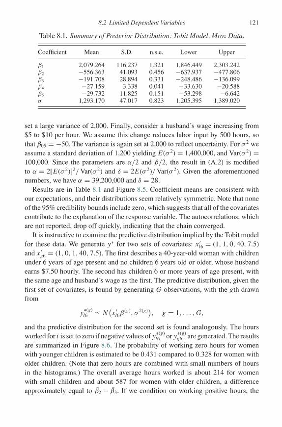
P1: KAE



Table 8.1. Summary of Posterior Distribution: Tobit Model, Mroz Data.

Coefficient Mean S.D. n.s.e. Lower Upper

β1 2,079.264 116.237 1.321 1,846.449 2,303.242β2 −556.363 41.093 0.456 −637.937 −477.806β3 −191.708 28.894 0.331 −248.486 −136.099β4 −27.159 3.338 0.041 −33.630 −20.588β5 −29.732 11.825 0.151 −53.298 −6.642σ 1,293.170 47.017 0.823 1,205.395 1,389.020

set a large variance of 2,000. Finally, consider a husband’s wage increasing from$5 to $10 per hour. We assume this change reduces labor input by 500 hours, sothat β05 = −50. The variance is again set at 2,000 to reflect uncertainty. For σ 2 weassume a standard deviation of 1,200 yielding E(σ 2) = 1,400,000, and Var(σ 2) =100,000. Since the parameters are α/2 and β/2, the result in (A.2) is modifiedto α = 2[E(σ 2)]2/ Var(σ 2) and δ = 2E(σ 2)/ Var(σ 2). Given the aforementionednumbers, we have α = 39,200,000 and δ = 28.

Results are in Table 8.1 and Figure 8.5. Coefficient means are consistent withour expectations, and their distributions seem relatively symmetric. Note that noneof the 95% credibility bounds include zero, which suggests that all of the covariatescontribute to the explanation of the response variable. The autocorrelations, whichare not reported, drop off quickly, indicating that the chain converged.

It is instructive to examine the predictive distribution implied by the Tobit modelfor these data. We generate y∗ for two sets of covariates: x ′

l6 = (1, 1, 0, 40, 7.5)and x ′

g6 = (1, 0, 1, 40, 7.5). The first describes a 40-year-old woman with childrenunder 6 years of age present and no children 6 years old or older, whose husbandearns $7.50 hourly. The second has children 6 or more years of age present, withthe same age and husband’s wage as the first. The predictive distribution, given thefirst set of covariates, is found by generating G observations, with the gth drawnfrom

y∗(g)l6 ∼ N

(x ′

l6β(g), σ 2(g)

), g = 1, . . . , G,

and the predictive distribution for the second set is found analogously. The hoursworked for i is set to zero if negative values of y

∗(g)l6 or y

∗(g)g6 are generated. The results

are summarized in Figure 8.6. The probability of working zero hours for womenwith younger children is estimated to be 0.431 compared to 0.328 for women witholder children. (Note that zero hours are combined with small numbers of hoursin the histograms.) The overall average hours worked is about 214 for womenwith small children and about 587 for women with older children, a differenceapproximately equal to β2 − β3. If we condition on working positive hours, the

P1: KAE



β2

π(β 2|y

)

400 300 200 100 0β

3

π(β 3|y

)

50 40 30 20 10β

4

π(β 4|y

)

80 60 40 20 0 20β

5

π(β 5|y

)

Figure 8.5. Posterior distributions of β: Tobit model, Mroz data.

mean is about 1,284 h for women with small children and 1,105 for women witholder children. In summary, having older rather than younger children increasesthe probability of working positive hours by about 0.100, and, for those who work,the average number of hours is increased by about 180 h.

8.2.2 Binary Probit Model

The binary probit model is designed to deal with situations in which yi can takeone of two values, coded as 0 and 1. For example, if y denotes union membership,let yi = 0 if person i does not belong to a union and yi = 1 if he or she does. Or yi

could denote a choice of one of the parties in a two-party election. Finally, yi mightequal 1 if subject i receives a treatment and 0 if not. Since y has the character ofa Bernoulli variable, we model its probability mass function, p(y), rather than y

itself.There is an interesting relationship between the linear regression model and a

model for binary data. The linear regression model assumes E(yi) = x ′iβ. This

assumption can be generalized to what statisticians call the generalized linearmodel (GLM) by specifying E(yi) = G(x ′

iβ), where G(·) is called the link function

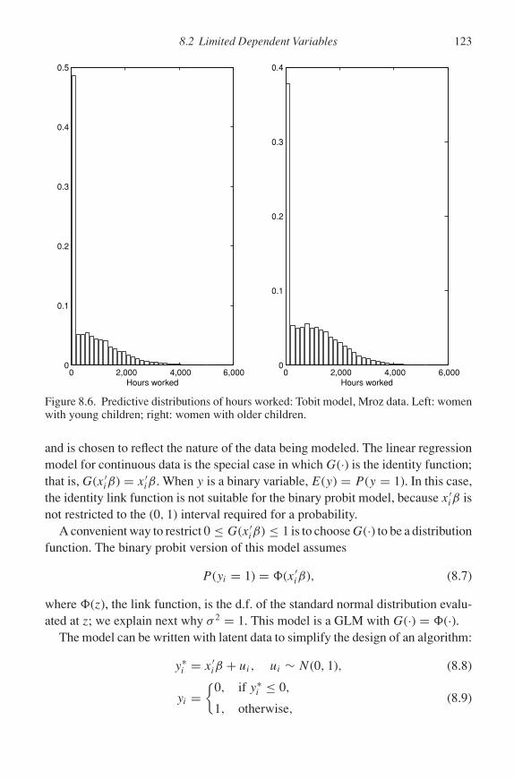
P1: KAE



0 2,000 4,000 6,0000

0.1

0.2

0.3

0.4

0.5

Hours worked0 2,000 4,000 6,000

0

0.1

0.2

0.3

0.4

Hours worked

Figure 8.6. Predictive distributions of hours worked: Tobit model, Mroz data. Left: womenwith young children; right: women with older children.

and is chosen to reflect the nature of the data being modeled. The linear regressionmodel for continuous data is the special case in which G(·) is the identity function;that is, G(x ′

iβ) = x ′iβ. When y is a binary variable, E(y) = P (y = 1). In this case,

the identity link function is not suitable for the binary probit model, because x ′iβ is

not restricted to the (0, 1) interval required for a probability.A convenient way to restrict 0 ≤ G(x ′

iβ) ≤ 1 is to choose G(·) to be a distributionfunction. The binary probit version of this model assumes

P (yi = 1) = �(x ′iβ), (8.7)

where �(z), the link function, is the d.f. of the standard normal distribution evalu-ated at z; we explain next why σ 2 = 1. This model is a GLM with G(·) = �(·).

The model can be written with latent data to simplify the design of an algorithm:

y∗i = x ′

iβ + ui, ui ∼ N(0, 1), (8.8)

yi ={

0, if y∗i ≤ 0,

1, otherwise,(8.9)

P1: KAE



or yi = 1(y∗i > 0). You should verify that the latent data form of the model is

equivalent to (8.7). The latent data formulation makes clear why we assume ui ∼N(0, 1), rather than the more general assumption N(0, σ 2). Since it is only the signof y∗

i that determines the observed yi , both sides of (8.8) can be multiplied by anynonnegative constant and still be consistent with the observed data, which showsthat the pair (β, σ 2) is not identified. A simple way to achieve identification is toset σ 2 = 1.

Determining the prior distribution for β is not as straightforward as it is inthe linear regression case, where βk is interpreted as ∂E(y)

∂xkfor continuous data. In

general,

∂E(y∗i )

∂xik

= βk

∂G(x ′iβ)

∂xik

,

and for the Gaussian link function,

∂E(y∗i )

∂xik

= βkφ(x ′iβ),

where φ(·) is the p.d.f. of the Gaussian distribution. The effect of xik on E(yi)therefore depends on the vector xi and all of the elements of β. One way toapproach the problem of assigning a prior distribution for β is to consider thevalue of x ′

iβ at which xik has the largest effect on yi . For the normal distribution,this occurs at x ′

iβ = 0, where φ(·) is maximized. Since φ(0) = 1/√

2π = 0.3989,the largest effect of xk on y is approximately 0.4βk; this fact may help to put aprior mean and variance on β. Note that P (yi = 1|β) = 0.5 at x ′

iβ = 0. Anotherapproach is to think about P (yi = 1|β) at various values of the covariates and setparameter values accordingly. This approach is illustrated in the example describedlater.

To specify a Gibbs algorithm for this problem, we add the latent data y∗ to thesampler as in Albert and Chib (1993b) and write the likelihood contribution of theith observation as

p(yi |y∗i ) = 1(yi = 0)1(y∗

i ≤ 0) + 1(yi = 1)1(y∗i > 0),

because yi = 0 ⇐⇒ y∗i ≤ 0. Assuming the usual Gaussian prior distribution for

β, we can write the posterior distribution of β and y∗ = (y∗1 , . . . , y∗

n)′ as

π (β, y∗|y) =∏

p(yi |y∗i )f (y∗

i |β)π (β)

=∏

[1(yi = 0)1(y∗i ≤ 0) + 1(yi = 1)1(y∗

i > 0)]

× Nn(y∗|Xβ, I )NK (β|β0, B0).


P1: KAE



Algorithm 8.3: Gibbs algorithm for binary probit

8.1 Choose a starting value β(0).8.2 At the gth iteration, draw

y∗(g)i ∼

{TN(−∞,0](x ′

iβ(g−1), 1), if yi = 0,

TN(0,∞)(x ′iβ

(g−1), 1), if yi = 1,i = 1, . . . , n,

β(g) ∼ NK (β(g), B1),

where

B1 = [X′X + B−1

0

]−1,

β(g) = B1[X′y∗(g)

i + B−10 β0

].

Note that B1 is not updated, because σ 2 = 1.Before turning to an example, we consider a model in which the link function

is the Student-t distribution with ν degrees of freedom. From our discussion inSection 8.1.2, it should be clear that this can be accomplished by the model

y∗i = x ′

iβ + ui, ui ∼ N(0, λ−1

i

), λi ∼ G(ν/2, ν/2).

The analysis proceeds by including λi and y∗i in the sampler.

We illustrate the probit model for binary data by applying it to computer owner-ship data collected by the U.S. Census Bureau and the Bureau of Labor Statisticsfrom a survey of a large number of U.S. households. This survey contains informa-tion on whether the household owns a computer, yi = 1, and detailed demographicinformation about the household. We extracted a random sample of 500 house-holds from the large number contained in this survey. The first task is to specifythe covariates for the model. We assume that computer ownership is influenced bywhether the person is a college graduate and the household’s income, measuredas the weekly wage of the household in thousands of dollars. We therefore definethe covariates xi2 as the weekly wage of household i and xi3 = 1 if the head ofhousehold i is a college graduate and zero if not. Since the observations are arandom sample of households, it is reasonable to assume that they are independent.Accordingly, the likelihood function is the product of the likelihood functions foreach household.

The next step is to specify the prior distribution of β. Consider a householdwith a zero weekly wage headed by a person who did not graduate college. Weassume a low probability, 0.10, that such a household contains a computer. Ac-cordingly,

∫ β1

−∞ φ(t) dt = 0.10. This implies β1 = −1.2816, which we take as β01.On the assumption that this probability is very likely to be less than 0.3, we solve∫ β1

−∞ φ(t) dt = 0.3 to find β1 = −0.5244. Interpreting “very likely” to mean a prob-ability of 0.95, we have (−0.5244 + 1.2816)/

√B0,11 = 1.96, or B0,11 = 0.1492.

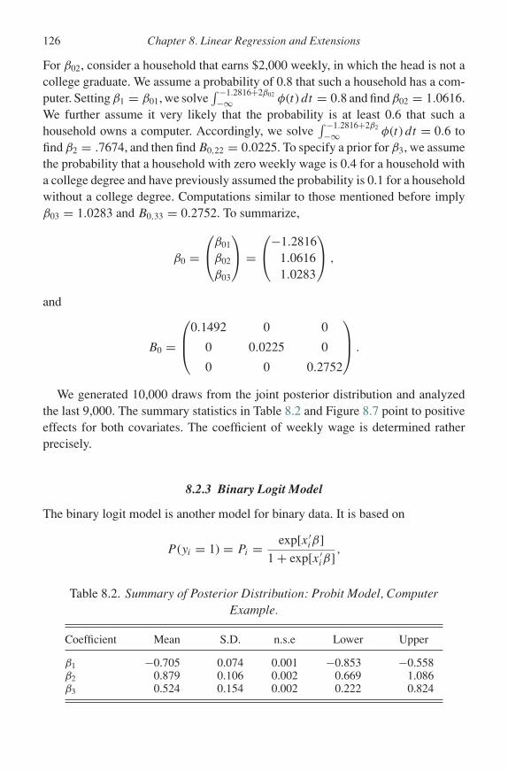
P1: KAE



For β02, consider a household that earns $2,000 weekly, in which the head is not acollege graduate. We assume a probability of 0.8 that such a household has a com-puter. Setting β1 = β01, we solve

∫ −1.2816+2β02

−∞ φ(t) dt = 0.8 and find β02 = 1.0616.We further assume it very likely that the probability is at least 0.6 that such ahousehold owns a computer. Accordingly, we solve

∫ −1.2816+2β2

−∞ φ(t) dt = 0.6 tofind β2 = .7674, and then find B0,22 = 0.0225. To specify a prior for β3, we assumethe probability that a household with zero weekly wage is 0.4 for a household witha college degree and have previously assumed the probability is 0.1 for a householdwithout a college degree. Computations similar to those mentioned before implyβ03 = 1.0283 and B0,33 = 0.2752. To summarize,

β0 =β01

β02

β03

=−1.2816

1.06161.0283

,

and

B0 =

0.1492 0 0

0 0.0225 0

0 0 0.2752

.

We generated 10,000 draws from the joint posterior distribution and analyzedthe last 9,000. The summary statistics in Table 8.2 and Figure 8.7 point to positiveeffects for both covariates. The coefficient of weekly wage is determined ratherprecisely.

8.2.3 Binary Logit Model

The binary logit model is another model for binary data. It is based on

P (yi = 1) = Pi = exp[x ′iβ]

1 + exp[x ′iβ]

,

Table 8.2. Summary of Posterior Distribution: Probit Model, ComputerExample.

Coefficient Mean S.D. n.s.e Lower Upper

β1 −0.705 0.074 0.001 −0.853 −0.558β2 0.879 0.106 0.002 0.669 1.086β3 0.524 0.154 0.002 0.222 0.824

P1: KAE



0.4 0.6 0.8 1 1.2 1.4β

2

π(β 2|y

)

5 0 0.5 1 1.5β

3

π(β 3|y

)

Figure 8.7. Posterior distributions of β: computer ownership example, probit model.

which implies the link function G(x ′iβ) = exp[x ′

iβ]/(1 + exp[x ′iβ]). This model

can be written in the form of latent data as

y∗i = x ′

iβ + ui,

where ui has the logistic distribution, P (Ui ≤ ui) = �(ui) = eui /(1 + eui ) anddensity function λ(ui) = eui /(1 + eui )2.

This model has the interesting property that

logit(Pi) ≡ log

(P (yi = 1)

P (yi = 0)

)= log

(Pi

1 − Pi

)= x ′

iβ,

that is, the logarithm of the odds ratio is a linear function of the covariates.This feature may be useful for setting prior distributions because it implies that∂ logit(Pi )

∂xik= βk, which permits the use of subject-matter based knowledge about the

effect on the log odds ratio of a change in a covariate. In addition, the generalresult ∂Pi

∂xik= βk

∂G(x ′iβ)

∂xikimplies that ∂Pi

∂xik= βkPi(1 − Pi) for the logit model. Since

this expression is maximized at Pi = 1/2, the largest effect of covariate k on theprobability is βk/4, a fact that may be helpful in specifying a prior distribution forβk. This calculation also allows a rough comparison between the coefficients of a

P1: KAE



probit and logit model fit to the same data. We saw in Section 8.2.2 that ∂Pi

∂xikis max-

imized at 0.4βpk, where βpk is the coefficient from a probit equation. Equating themaximum effects, we have 0.4βpk = βlk/4, or the logit coefficient βlk = 1.6βpk.This approximation should be reasonably good in the neighborhood of x ′

iβ = 0.Placing a normal prior on β results in a model that is not conditionally conjugate;

see Exercise 8.8. Since the conditional posterior distribution of β is not a standardform, we utilize the general form of the MH algorithm to approximate it. A possibleproposal generator is the random walk, in which a scaled normal or Student-tvariable is added to the current value; another possibility is an independence chain,where the proposal density is a Student-t distribution centered at the maximumof the posterior distribution with scale matrix proportional to the negative of theinverted Hessian at the maximum.

We illustrate the logit model by returning to the computer ownership data dis-cussed earlier. That discussion leads us to specify the likelihood function

Pi = exp[β1 + β2xi2 + β3xi3]

1 + exp[β1 + β2xi2 + β3xi3],

where the covariates are defined earlier. The likelihood function for the sample isagain the product of the individual likelihoods.

To specify prior distributions for the βk, we start with the result that logit(Pi) =x ′

iβ and consider a household with zero income and a head of household whois not a college graduate. In that case logit(Pi) = β1. We assume that such ahousehold has a small probability of owning a computer, say 0.1, implying thatlog(1/9) = −2.1972, which is taken as the mean of the prior distribution for β1.If we consider it very unlikely that the probability is greater than 0.3, log(3/7) =−0.8473 is taken to be the upper end of the interval that contains 95% of theprobability distribution of β1. This implies a prior standard deviation of β1 of√

B0,11 = [−0.8473 − (−2.1972)]/1.96 = 0.6887, or a variance B0,11 = 0.4743.For β2, let us consider a household with a weekly wage of $2,000 and a head

of household who is not a college graduate. We assume the probability is 0.8 thatsuch a household owns a computer. Since the wage is measured in thousands,log(8/2) = −2.1972 + 2β2, which implies β02 = 1.7917. If we take 0.6 as thelower limit of a 95% credibility interval for the probability that a household earning$2,000 per week owns a computer, we find that the variance of the prior density ofβ2, B0,22, is 0.2504.

The last coefficient gives the effect of being a college graduate. Assume againa household with a weekly income of zero and consider the logit of a householdin which the head has a college degree, β1 + β3, compared to one in which thehead does not have a degree, β1. We have taken the latter to be 1/9 and assumethe former to be 0.4; these imply that β3 = 0.3. On the assumption that this effect

P1: KAE



is not likely to be greater than 0.5, we find an implied standard deviation of one.Accordingly, B0,33 = 1.

In summary, under the assumption that the parameters are independent andnormally distributed, our prior distribution is

π (β0) = N(β|β0, B0), (8.10)

where

β0 =β01

β02

β03

=−2.1972

1.79170.3000

,

and

B0 =

0.4743 0 0

0 0.2504 0

0 0 1.000

.

We generate a sample of 10,000 from the posterior distribution and discard 1,000as the burn-in. The autocorrelations are very low, resulting in values of both r.n.e.and autocorrelation time close to one. A summary of the output is in Table 8.3,and Figure 8.8 presents histograms of the posterior distributions of β2 and β3. Thesample results yield P (β2 > 0|y) = 0.98 and P (β3 > 0|y) = 0.88, which suggeststhat income almost certainly has an effect but that the positive effect on computerownership of being a college graduate is less clear.


Chapter 8 Appendix B contains comments on computer programs for performingthe computations discussed in this chapter.

Section 8.1.1 Special algorithms have been devised to deal with the problem ofmodel selection when a researcher contemplates a linear regression model witha large number of possible covariates and little prior information about which ofthese to include. The overall model in this case includes a possibly large number of

Table 8.3. Summary of Posterior Distribution: Logit Model, Computer Example.


β1 −1.081 0.382 0.004 −1.818 −0.305β2 1.299 0.636 0.007 0.027 2.557β3 0.786 0.745 0.007 −0.703 2.230

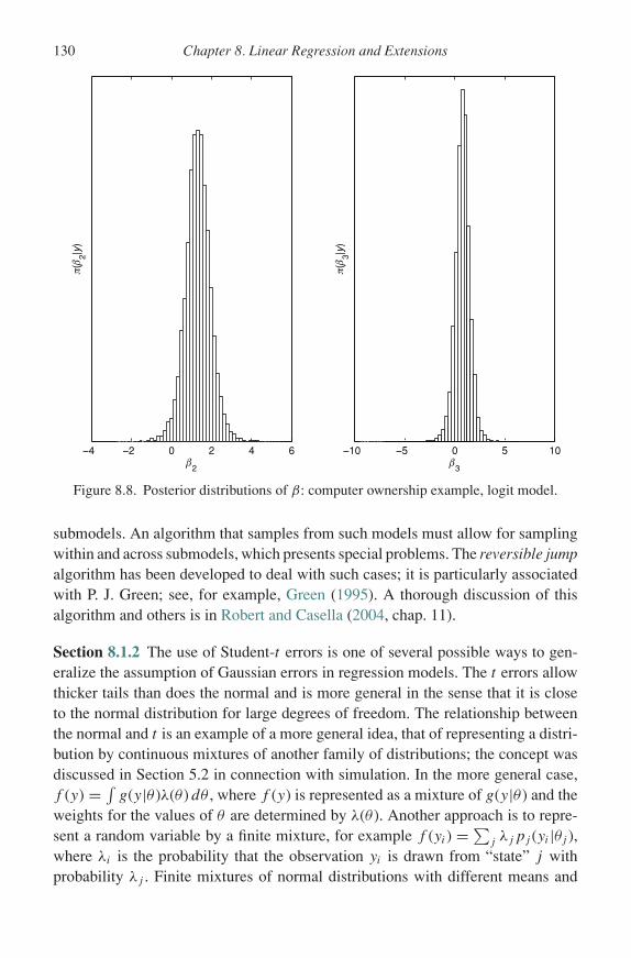
P1: KAE



0 2 4 6β

2

π(β 2|y

)

10 5 0 5 10β

3

π(β 3|y

)

Figure 8.8. Posterior distributions of β: computer ownership example, logit model.

submodels. An algorithm that samples from such models must allow for samplingwithin and across submodels, which presents special problems. The reversible jumpalgorithm has been developed to deal with such cases; it is particularly associatedwith P. J. Green; see, for example, Green (1995). A thorough discussion of thisalgorithm and others is in Robert and Casella (2004, chap. 11).

Section 8.1.2 The use of Student-t errors is one of several possible ways to gen-eralize the assumption of Gaussian errors in regression models. The t errors allowthicker tails than does the normal and is more general in the sense that it is closeto the normal distribution for large degrees of freedom. The relationship betweenthe normal and t is an example of a more general idea, that of representing a distri-bution by continuous mixtures of another family of distributions; the concept wasdiscussed in Section 5.2 in connection with simulation. In the more general case,f (y) = ∫

g(y|θ )λ(θ ) dθ , where f (y) is represented as a mixture of g(y|θ ) and theweights for the values of θ are determined by λ(θ ). Another approach is to repre-sent a random variable by a finite mixture, for example f (yi) = ∑

j λjpj (yi |θj ),where λi is the probability that the observation yi is drawn from “state” j withprobability λj . Finite mixtures of normal distributions with different means and

P1: KAE



variances can display a wide variety of shapes. See Gelman et al. (2004, chap. 18)and Geweke (2005, sec. 6.4) for more discussion of such mixtures. The latterdiscusses estimation of the model by procedure “fmn ullm” in BACC.

Another general approach to modeling error terms flexibly is the Dirichlet mix-ture process. See Escobar and West (1995) for a discussion and references and anMCMC approach to simulation. A method of computing the marginal likelihoodfor such models is presented in Basu and Chib (2003).

Section 8.2 Greene (2003, chaps. 21 and 22) presents the Tobit and binary probitmodels in a frequentist setting, including explicit formulas for the Hessian matricesand a comparison of the coefficients of probit and logit models. Wooldridge (2002,chaps. 15 and 16) also covers these models in great detail. He points out animportant difference between the top-coded and boundary solution versions of theTobit model: the values of β are of interest in the former because E(y∗|x) = x ′βcan be interpreted as an expectation in the absence of top coding, and so β has itsusual interpretation as a partial derivative. In contrast, for the boundary solutioncase, interest usually centers on E(y|x), E(y|x, y > 0), or P (y = 0|x), rather thanβ, because values of y∗ < 0 have no meaning. An exception arises in the utilitymaximization model, where β may depend on parameters of the utility function.The probit and logit models are thoroughly covered by Train (2003), who includesa Bayesian analysis of the latter.

Tanner and Wong (1987) introduce the idea of introducing missing data in atwo-block Gibbs sampling algorithm. In the first application of MCMC methodsto econometrics, Chib (1992) analyzes the Tobit model. The use of latent data ina Gibbs algorithm by Albert and Chib (1993b) for the binary probit model andthe ordered probit and Student-t versions of the model has become the standardapproach to categorical responses from a Bayesian perspective. Chib and Greenberg(1998) show how the approach extends to correlated binary data.

An interesting variation of the binary probit model appears in the politicalscience literature in the form of the spatial voting model, which is equivalent tothe two-parameter item response model used in educational testing. The statisticalmodel takes the form

P (yij = 1) = �(β ′j xi − αj ), (8.11)

where yij is 1 if legislator i votes yea on issue j and 0 otherwise, i = 1, . . . , n,j = 1, . . . , m. The d × 1 vector xi represents i’s “ideal point,” which is the primaryobject of interest of the analysis. The only data observed are the yij , and d(d + 1)restrictions must be imposed on X = (x ′

1, . . . , x′n)′ to identify the remainder of X,

the βj , and the αj . The Bayesian approach to the spatial voting model is explainedin Clinton et al. (2004) who assume Gaussian priors for the xi , βj , and αj . A

P1: KAE



dynamic version of this model is analyzed in Martin and Quinn (2002), where theideal points are given a time index, xit , and are allowed to evolve. Models in whichparameters evolve over time are discussed in Section 10.3.

Generalizations of the binary probit and logit models to data sets in which anindividual chooses among three or more possibilities are discussed in Section 9.4.

8.4 Exercises

8.1 Download the data in “Birth weight II” from the StatLabs Web site, www.stat.berkeley.edu/users/statlabs/labs.html. The variables are birth weight (ounces, 999 unknown),gestation (length of pregnancy in days, 999 unknown), parity (0 = firstborn, 9 isunknown), age (mother’s age in years), height (mother’s height in inches), weight(mother’s prepregnancy weight in pounds), smoke (0 not now, 1 yes now, 9 = un-known).

Specify a linear regression, where the response variable is birth weight, and thecovariates are a constant and the remaining variables in the data set. Eliminate ob-servations for which you do not have complete information on the variables. Specifyprior distributions for the coefficients and the variance (or precision). Summarize theresults for the dummy variable for smoking. Does smoking by the mother appear toaffect the baby’s birth weight?

8.2 Verify that specifying the model of (8.4) by a Student-t likelihood function on ν

degrees of freedom for y, a normal prior for β, and an inverse gamma prior for σ 2

does not permit use of the Gibbs algorithm. Verify that a Student-t likelihood functionon ν degrees of freedom for y and a Student-t prior for β do not yield conditionaldistributions that permit a Gibbs algorithm.

8.3 Repeat Exercise 8.1 for errors distributed as Student-t with five degrees of freedom.Compute marginal likelihoods and compare the models.

8.4 Study the sensitivity of the results for the union coefficient by varying the prior meanand variance.

8.5 Write out an algorithm to sample for β, σ 2, and λ for the linear regression model withStudent-t errors of Section 8.1.2.

8.6 Write out an algorithm to sample for β, σ 2, y∗Ci , and λ for the Tobit model of

Section 8.2.1 with Student-t errors.8.7 Write out an algorithm to sample for β, y∗, and λ for the binary data model with

Student-t errors of Section 8.2.2.8.8 Verify that the posterior distribution of the logit model with a normal prior (Sec-

tion 8.2.3) has the form

π (β|y) ∝∏(

exp[x ′iβ]

1 + exp[x ′iβ]

)yi(

1

1 + exp[x ′iβ]

)1−yi

× exp

[− 1

2(β − β0)′B−1

0 (β − β0)

],

P1: KAE


8.4 Exercises 133

and show that including the latent data in the sampler does not simplify the posteriordistribution.

8.9 Write out an algorithm to estimate the parameters of (8.11) under the Gaussian prior.Compare your algorithm to the one in Clinton et al. (2004).

8.10 Another type of discrete data is count data, where the observations yi are equal tozero or a positive integer; that is, yi ∈ {0, 1, . . . }. Such data are often modeled bythe Poisson distribution,

p(yi |θi) = e−θi θyi

i

yi!, θi = exp(x ′

iβ).

The model is discussed in detail from the frequentist viewpoint in Wooldridge(2002, chap. 19) and Winkelmann (1997); the latter also discusses the Bayesianapproach. Find an expression for the posterior distribution β|y on the assumptionthat π (β) = N (β0, B0), and discuss possible ways to simulate from this distribution.(See Winkelmann, 1997, sec. 5.2.1.)

P1: KAE


Chapter 9

Multivariate Responses

IN THIS CHAPTER, we consider three examples of models in which the responsevariable is a vector, rather than a scalar, random variable: the “seemingly unrelatedregression” (SUR) model, the multivariate probit (MVP) model, and a model forpanel data.

9.1 SUR Model

The SUR model was introduced in Zellner (1962) and has been applied extensively.Before turning to examples we specify the model formally. Since the responsevariable is multivariate, the observations and error terms are written with twosubscripts:

ysj = x ′sjβs + usj , s = 1, . . . , S, j = 1, . . . , J, (9.1)

where xsj is Ks × 1 and βs = (βs1, βs2, . . . , βsKs)′. The j th observation on the

vector of responses is contained in the S × 1 vector yj = (y1j , y2j , . . . , ySj )′. Tospecify a model for yj , we define the S × K matrix, K = ∑

Ks ,

Xj =

x ′

1j . . . 0

0 x ′2j . . . 0

...

0 0 . . . x ′Sj

,

the K × 1 vector β = (β ′1, . . . β

′S)′, and the S × 1 vector uj = (u1j , u2j , . . . uSj )′;

these definitions and the model specification imply

yj = Xjβ + uj . (9.2)

The defining characteristic of the SUR model is the assumption that uj |X ∼NS(0, ), where X = (X1, . . . , XJ ) and = {σst}. The covariances permit

134

P1: KAE


9.1 SUR Model 135

nonzero correlations for disturbances with the same second subscript,

Cov(usj , utk|X) ={

σst , if j = k,

0, otherwise.

These nonzero covariances explain the phrase “seemingly unrelated.” If the co-variances were all zero, each of the equations in (9.2) would be unrelated to theothers. But the nonzero covariances tie the individual regressions into a system ofequations that can be analyzed together. Finally, note that the model allows thedisturbance variances σss to differ across firms and that the uj |X are independentacross j , that is,

f (u1, . . . , uJ |X) = f (u1|X) · · · f (uJ |X).

Here are examples of data sets to which the model has been applied:

9.1 Let ysj be the investment expenditures of firm s in year j , where all of the firms are inthe same industry. In that case, usj represents unobserved disturbances that affect firms at time j . Since the firms are in the same industry, it is reasonable to assume thata disturbance in a particular period affects all the firms to some degree, which can bemodeled by assuming that the covariance σst between the disturbances of firms s andt at time j is not zero. Finally, the specification assumes that the disturbances acrosstime for a given firm are independent.

9.2 Let ysj represent the score on the sth of one of several medical or intelligence tests takenby individual j . The specification permits the scores to be correlated for a particularindividual, perhaps representing some unobserved genetic factor, but the scores acrossindividuals are independent.

9.3 Let ysj represent the expenditures by household s on product j . The specification allowsthe disturbance to expenditures across product categories for a particular household tobe correlated, but assumes zero correlation across households.

Before turning to the analysis of this model, we note a special case,

ysj = x ′sjβ + usj ,

where xsj is defined as before, but β is a K × 1 vector. This specification differsfrom (9.1) by assuming that all the βs are equal to the common value β. The specialcase is still a SUR model because of the assumption that σst = 0. By defining

Xj =

x ′

1j

x ′2j

...

x ′Sj

,

and β = (β1, . . . , βk)′, verify that (9.2) is still valid.

P1: KAE


136 Chapter 9. Multivariate Responses

From the specification of the SUR model and the definition of the multivariatenormal distribution in Section A.1.12, the likelihood function for the data y =(y1, . . . , yJ ) is

f (y|β, ) ∝ 1

||J/2exp

−1

2

∑j

(yj − Xjβ)′−1(yj − Xjβ)

. (9.3)

We next specify a conditionally conjugate prior for this model. The regressioncoefficients are assumed to have a Gaussian prior, β ∼ NK (β0, B0). For the pre-cision matrix −1, we assume a generalization of the gamma distribution, theWishart distribution described in Section A.1.16: −1 ∼ WS(ν0, R0). (We couldhave equivalently assumed an inverted Wishart distribution for the covariancematrix .)

With these assumptions, the posterior distribution is

π (β, |y) ∝ 1

||J/2exp

−1

2

∑j

(yj − Xjβ)′−1(yj − Xjβ)

× exp

[−1

2(β − β0)′B−1

0 (β − β0)

]× 1

||(ν0−S−1)/2exp

[−1

2tr(R−1

0 −1)

].

It is then straightforward to determine the conditional distribution,

β|y, ∼ NK (β, B1),

where

B1 =[∑

j

X′j

−1Xj + B−10

]−1

,

β = B1

[∑j

X′j

−1yj + B−10 β0

].

(9.4)

To derive the conditional distribution of |y, β we use the properties of the traceoperator z′Az = tr(z′Az) = tr(zz′A), where z is a column vector, to obtain∑

j

(yj − Xjβ)′−1(yj − Xjβ) = tr∑

j

(yj − Xjβ)(yj − Xjβ)′−1,

P1: KAE


9.1 SUR Model 137

from which we immediately have |y, β ∼ WS(ν1, R1), where

ν1 = ν0 + J,

R1 =[R−1

0 +∑

j

(yj − Xjβ)(yj − Xjβ)′]−1

.(9.5)


Algorithm 9.1: Gibbs algorithm for SUR model

9.1 Choose a starting value (0).9.2 At the gth iteration, draw

β(g) ∼ NK

(β(g), B

(g)1

)−1(g) ∼ WS

(ν1, R

(g)1

),

where β(g) and B(g)1 are given in (9.4) with −1 replaced by −1(g−1), and ν1 and R

(g)1

are given in (9.5) with β replaced by β(g).

As an application of this model, we consider the Grunfeld (1958) study ofinvestment behavior as discussed in Boot and de Wit (1960), where the data maybe found. In this model, gross investment including repairs and maintenance (It )is the response variable, and the covariates are a constant, the market value ofthe firm (Ft ), and the firm’s capital stock (Ct ). The variables are deflated byappropriate price indices, and the data are for the years 1935–1954 for five largemanufacturing companies: General Motors (GM), Chrysler (C), General Electric(GE), Westinghouse (W), and U.S. Steel (USS). We consider the SUR version ofthe model M1, where the βs differ for each firm and contemporaneous correlationsare permitted, and a version M2 in which the βs differ, but contemporaneouscorrelations are forced to equal zero. For a third model, M3, we assume zerocontemporaneous correlations and the same βs for each firm.

Boot and de Wit (1960, p. 8) offer a few comments about parameter values for βsF

and βsC that can be used to form prior distributions. On the basis of their discussion,we assume each βsF ∼ N(0, 0.33) and each βsC ∼ N(0.25, 0.17). These imply that−1 ≤ βF ≤ 1.0 with probability 0.997 and that 0 ≤ βC ≤ 1 with probability 0.997.There is little prior information about the constant term. We assume β1 ∼ N(0, 100)as an uninformative prior. To allow for uncertainty in the distribution of , we setν0 = 6, and we set R0 = 400I5 to allow for large variances of the disturbances. ForM2 and M3, we assume the precision is distributed as G(1, 1/400), and the priorsfor the βs are the same as those of M1.

The results for M1 in Figures 9.1 and 9.2 and Tables 9.1–9.3 indicate considerablevariation in βF and βC across firms and values of contemporaneous correlations

P1: KAE



GM C GE W USS

0

0.05

0.1

0.15

0.2

β F

Figure 9.1. Summary of βF .

ranging in absolute value from 0.029 to 0.599. The β values for M2 show compa-rable variation. The marginal likelihood values are −708.60 for M1, −593.01 forM2, and −651.75 for M3. By this criterion, the data strongly favor M2, a model thatallows each firm to have a different set of regression coefficients, but imposes zerocontemporaneous correlations. Another model that might be examined is one inthat permits different regression coefficients and different variances for each firm.This possibility is included as an exercise.

One reason why M1 lost so decisively to M2 may have to do with the number ofparameters in the model, as discussed in Section 3.2.4. Both M1 and M2 contain 15regression coefficients, but the former also contains 5 variances and 10 covariances,

Table 9.1. Summary of Posterior Distribution of βF : Grunfeld Data, SUR Model.

Firm Mean S.D. n.s.e. Lower Upper

GM 0.084 0.008 0.000 0.069 0.099C 0.071 0.012 0.000 0.047 0.094GE 0.030 0.007 0.000 0.017 0.045W 0.052 0.008 0.000 0.036 0.068USS 0.153 0.020 0.000 0.114 0.191

P1: KAE


9.2 Multivariate Probit Model 139

GM C GE W USS

2

1

0

0.1

0.2

0.3

0.4

0.5

0.6

0.7

β C

Figure 9.2. Summary of βC .

whereas M2 includes only one variance. The latter model therefore entails 14 fewerparameters than does the former. Although we might expect the likelihood ratioto favor the model with more parameters, M1, the effect from this source wasapparently not enough to offset the larger number of parameters. In contrast,M3, which contains only four parameters, is decisively beaten by M2 with its 16parameters.

9.2 Multivariate Probit Model

The multivariate probit (MVP) model is a SUR model in which all response vari-ables are binary choices: yij = 1 indicates that individual i chooses 1 on decision

Table 9.2. Summary of Posterior Distribution of βC: Grunfeld Data, SUR Model.

Firm Mean S.D. n.s.e. Lower Upper

GM 0.394 0.037 0.000 0.322 0.469C 0.309 0.028 0.000 0.254 0.364GE 0.114 0.026 0.000 0.062 0.163W 0.032 0.042 0.000 −0.052 0.112USS 0.337 0.114 0.002 0.116 0.566

P1: KAE



Table 9.3. Means of Posterior Distribution of ContemporaneousCorrelations: Grunfeld Data, SUR Model.

1.000 0.073 −0.151 −0.370 0.5560.073 1.000 0.126 0.029 −0.297

−0.151 0.126 1.000 −0.562 −0.091−0.370 0.029 −0.562 1.000 −0.599

0.556 −0.297 −0.091 −0.599 1.000

j , and yij = 0 indicates that individual i chooses 0 on decision j , i = 1, . . . , n,j = 1, . . . , J . It is applied to data sets in which decision maker i makes binarychoices over J decisions that are believed to be related through unobserved randomvariables. The model is most easily represented and analyzed by the latent variablerepresentation,

y∗ij = x ′

ijβj + uij ,

where xij and βj are Kj × 1, and let K = ∑Kj . The observed choices are the yij ,

which are related to the latent data through

yij ={

0, if y∗ij ≤ 0,

1, otherwise.

Upon defining y∗i = (y∗

i1, . . . , y∗iJ )′,

Xi =

x ′i1 0 . . . 0

0 x ′i2 . . . 0

0 0 . . . x ′iJ

,

β = (β ′1, . . . , β

′J )′, and ui = (ui1, . . . , uiJ )′, we can write

y∗i = Xiβ + ui.

Note that the observations are grouped by the first subscript in contrast to the SURmodel, where they were grouped by the second subscript. Grouping by the firstsubscript simplifies the writing of the likelihood function.

As an example of this model, consider individual i who makes two binarychoices: (1) send his or her child to a public or private school and (2) vote for oragainst a school tax increase. We might expect these choices to be related evenafter controlling for such covariates as income and family size.

We now continue with the specification of the model. The “probit” in MVParises from the assumption that ui ∼ NJ (0, ). The covariance matrix is notidentified for the MVP model, because only the signs of the latent variables areidentified through the likelihood function. In Section 8.2.2, we resolved the lack

P1: KAE



of identification by setting σ11 = 1. In the present case, we have J variances thatare not identified. One possibility is to set σjj = 1, j = 1, . . . , J . If J = 3, forexample,

=

1 σ12 σ13

σ12 1 σ23

σ13 σ23 1

.

With ones on the main diagonal, is a correlation matrix, and, because itis symmetric, there are J (J − 1)/2 unique unknown σij . We denote these byσ = (σ12, σ13, . . . , σJ−1,J )′. In addition, the positive definiteness of imposesrestrictions on σ .

We assume a Gaussian prior, β ∼ NK (β0, B0). For the elements of σ , we proposea normal prior, truncated to the region C in which is positive definite, so that1( ∈ C) = 1 if is positive definite and 0 otherwise. Then

π (σ ) ∝ 1( ∈ C) exp

[− 1

2(σ − σ0)′−1

0 (σ − σ0)

].

We can therefore write the posterior distribution as

π (β, , y∗|y) ∝ 1

||n/2exp

[−1

2

∑i

(y∗i − Xiβ)′−1(y∗

i − Xiβ)

]×∏i,j

[1(yij = 1)1(y∗ij > 0) + 1(yij = 0)1(y∗

ij ≤ 0)]

× exp

[−1

2(β − β0)′B−1

0 (β − β0)

]× 1( ∈ C) exp

[− 1

2(σ − σ0)′−1

0 (σ − σ0)

],

which implies

β|y, , y∗, y ∼ NK (β, B1), (9.6)

where

B1 =[∑

i

X′i

−1Xi + B−10

]−1

,

β = B1

[∑X′

i−1y∗

i + B−10 β0

].

(9.7)

The regression parameter β can therefore be simulated from its conditional distri-bution in a Gibbs step.

P1: KAE



The conditional posterior distribution for σ is

π (σ |y, y∗, β) ∝ 1( ∈ C)1

||n/2exp

[−1

2

∑i

(y∗i − Xiβ)′−1(y∗

i − Xiβ)

]

× exp

[−1

2(σ − σ0)′−1

0 (σ − σ0)

]. (9.8)

This distribution can be sampled by a tailored MH algorithm. The proposal densityat the gth iteration is a Student-t distribution with ν degrees of freedom (e.g.,ν = 5), with mean at the value of σ that maximizes the logarithm of Equation (9.8)given the current values of β and y∗. The scale matrix is taken to be the negativeof the inverse Hessian at the maximum. A draw from the distribution that violatesthe positive definiteness of is immediately rejected, and the current value of isretained. If the draw results in positive-definite , the proposed value replaces thecurrent value with the usual MH probability. Details are given in the next algorithm.

The y∗i are drawn from their full conditional posterior distributions, which are

independent truncated multivariate normal distributions, NJ (Xiβ, ), truncated tothe left at zero for j such that yij = 1 and to the right at zero for j such thatyij = 0. To make this draw we employ a Gibbs algorithm that cycles through thefull conditionals for i = 1, . . . , n,

f (y∗i1|y∗

i2, . . . , y∗iJ )

...f (y∗

ij |y∗i1, . . . , y

∗i,j−1, y

∗i,j+1, . . . , y

∗iJ )

...f (y∗

i,J |y∗i1, . . . , y

∗i,J−1),

(9.9)

where updated values of y∗ij are entered into the conditioning set as they are

generated. Each of these is a truncated univariate normal distribution with meanand variance given by the conditional distribution of (A.9).

In algorithmic form, we have

Algorithm 9.2: MH algorithm for MVP model

9.1 Select starting values y∗(0) and β(0).9.2 At the gth iteration,

(a) Maximize

− n

2log || − 1

2

∑i

(y

∗(g−1)i − Xiβ

(g−1))′

−1(y

∗(g−1)i − Xiβ

(g−1))

− 1

2(σ − σ0)′−1

0 (σ − σ0)

P1: KAE



with respect to σ . Denote the maximizing value by σ (g) and denote the negative ofthe inverse Hessian matrix at the maximizing value by S(g).

(b) Draw σ ∗ from tJ (J−1)/2(ν, σ (g), S(g)) and set

α(σ (g−1), σ ∗) =( ∏

i NJ (yi |Xiβ,∗)∏i NJ (yi |Xiβ,(g−1))

)(NJ (J−1)/2(σ ∗|σ0, 0)

NJ (J−1)/2(σ (g−1)|σ0, 0)

)×(

tJ (J−1)/2(σ ∗|ν, σ (g), S(g))

tJ (J−1)/2(σ (g−1)|ν, σ (g), S(g))

).

In these expressions, NJ (z|µ,) denotes the density function of the J -dimensionalnormal distribution with mean vector µ and covariance matrix evaluated at z;tD(t |ν, µ,) denotes the density function evaluated at t of the D-dimensionalStudent-t distribution with ν degrees of freedom, location vector µ, and scale matrix; and ∗ is the covariance matrix obtained from the covariances in σ ∗.

(c) Draw U from U (0, 1). If U ≤ α(σ (g−1), σ ∗), set σ (g) = σ ∗; otherwise, set σ (g) =σ (g−1). Note that a drawing of σ ∗ that leads to a that is not positive definite isalways rejected.

(d) Draw β(g) from (9.6), with = (g) and y∗ = y∗(g−1) in (9.7).(e) Draw y∗(g)|y, β(g), (g) following the strategy described around (9.9).

As an example, we consider a data set analyzed by Rubinfeld (1977). Ninety-five individuals report on whether they send at least one of their children to apublic school (yi1) and whether they voted in favor of a school tax increase (yi2).These decisions are modeled in the multivariate probit form. The covariates for thefirst decision are a constant, log(income), and log(property taxes); for the second,they are a constant, log(income), log(property taxes), and the number of years theresponder has lived in the city.

Some experimentation indicated considerable sensitivity of results to the priordistributions of the parameters. This is not surprising in view of the small samplesize. For this reason, we decided to impose highly uninformative priors: β0 =0, B0 = 100I7, and σ12 ∼ N(0, 0.5). We generated 5,500 observations, of which500 were discarded, and found autocorrelations at lag 20 to be very small. Theprior and posterior distributions are summarized in Table 9.4. The 95% credibilityintervals of most parameters range from negative to positive values, except thatβ22 seems clearly positive and β23 clearly negative. It appears that a higher incomeis associated with a higher probability of voting for a tax increase, while a higherproperty tax works in the opposite direction. Little can be said about the effects ofthe other covariates in the model.

P1: KAE



Table 9.4. Summary of Prior and Posterior Distributions of β and σ12: RubinfeldData.

Coefficient Prior Posterior

Mean S.D. Mean S.D. n.s.e. Lower Upper

β11 0.000 10.000 −4.543 3.761 0.230 −12.846 2.304β12 0.000 10.000 0.129 0.439 0.040 −0.698 0.994β13 0.000 10.000 0.620 0.607 0.037 −0.627 1.784β21 0.000 10.000 −0.634 3.762 0.309 −8.145 6.231β22 0.000 10.000 1.113 0.443 0.044 0.282 1.997β23 0.000 10.000 −1.437 0.546 0.050 −2.495 −0.367β24 0.000 10.000 −0.018 0.015 0.000 −0.048 0.013σ12 0.000 0.707 0.085 0.185 0.023 −0.302 0.455

9.3 Panel Data

Panel data consist of observations on the same unit over several time periods. Theresponse variable is denoted yit , which denotes an observation on unit i at time t .Since the first of the examples of SUR data mentioned in Section 9.1 also involvesindividual units across time, we discuss how the models differ before presentingthe panel data model in detail.

The SUR model is usually applied to data for which the number of time periodsis large and the number of units is small, and the panel data model is applied todatasets with a small number of time periods and a large number of units. Thefirst subscript of the response variable in the SUR model is usually associatedwith an identifiable unit whose behavior is expected to differ from that of otherunits, and such differences are of interest. In the investment data, for example,the s subscript identifies one of a small number of firms, and differences in theinvestment behavior of the firms are of interest in the research. The j subscriptindicates a year, and it is assumed that there are a large number of observationsfor the investment expenditures of each firm. In fact, there are usually enoughobservations to estimate individual regressions for each firm. As we have pointedout, it is the correlation across firms in a particular year that distinguishes the SURmodel from other models for multivariate data.

Although our other examples for SUR data do not involve time series cross-section data, they have the same general structure: in the test score example, thereare a fairly small number of tests and a large number of individuals, and we assumecorrelation across test results for a particular individual; we are also likely to believethat each covariate has a different effect on each test, which is indicated by differentvalues of βs . In the household expenditure example, there are a relatively small

P1: KAE


9.3 Panel Data 145

number of expenditure categories, indexed by s, and a large number of households,indexed by j , and we expect correlation across categories for a given household;again, the covariates are likely to affect each product differently. These cases havein common the idea that the first subscript of ysj is of particular interest and thatthe second indexes a relatively large number of observations.

In contrast, a typical panel data set consists of a large number of units, usuallyfirms or households, often over a time period that is too short to estimate a separateregression for each unit. The identity of the individual units is of no inherentinterest; they are chosen randomly from a very large population and are regarded asexchangeable. The large number of units makes it impractical to estimate individualvariances for each unit and covariances for each pair of units. This model assumesfurther that the behavior of the units is independent at each time period, but thatthere are differences across individuals that persist over time. These differences arecalled heterogeneity, and they are modeled by a nonzero covariance between thedisturbances of a particular firm or household across time.

Here are a few examples of panel data:

9.1 In a famous study, Mundlak (1961) considered agricultural production functions al-lowing for the possibility of unobserved differences in the quality of management orland that do not change over time.

9.2 Hausman (1978) considered log wages as a function of demographic variables in apanel of 629 observations over 6 years.

9.3 The Vella and Verbeek (1998) study, discussed in earlier chapters, is based on paneldata; the sample includes observations on 545 young men over 8 years.

A general version of the model may be written as

yit = x ′itβ + w′

it bi + uit , i = 1, . . . , n, t = 1, . . . , T , (9.10)

where xit and β are K1 × 1 and wit and bi are K2 × 1. The i subscript of bi

allows each of the variables in wit to have a different effect on each observationunit; these different effects are a way to model heterogeneity. It is assumed thatuit ∼ N(0, h−1

u ) and that Cov(uit , ujs) = 0 unless i = t and j = s. Note that thedistribution of uit has been parameterized in terms of the precision rather thanthe variance. We assume that the covariates in wit are a subset of those in xit . Inthe statistical literature, the elements of β, which do not differ across i, are calledfixed effects, and the bi , which do differ across i, are called random effects. Thisterminology differs from that found in most econometric discussions of panel datamodels. In that literature, the bi are regarded either as random variables and called“random effects,” or as nonrandom, but unknown, parameters and called “fixedeffects.” Since, from the Bayesian viewpoint, both β and the bi are regarded asrandom variables, the econometric terminology does not distinguish between the

P1: KAE



two types of parameters. We therefore adopt the definitions found in the statisticsliterature.

To illustrate how to apply the Bayesian approach to panel data, we specify abasic model and then discuss several ways in which it may be extended. First,define yi = (yi1, . . . , yiT )′, Xi = (xi1, . . . , xiT )′, ui = (ui1, . . . , uiT )′, and Wi =(wi1, . . . , wiT )′. Then the basic model is

yi = Xiβ + Wibi + ui,

ui |hu ∼ NT (0, h−1u IT ),

β ∼ NK1 (β0, B0),

hu ∼ G(α0/2, δ0/2),

bi |D ∼ NK2 (0, D),

D−1 ∼ WK2 (ν0, D0).

(9.11)

From the result that the posterior distribution is proportional to the likelihoodfunction times the prior distribution, we have

π (β, b, hu, D|y) ∝ hnT/2u exp

[−hu

2

∑(yi − Xiβ − Wibi)

′(yi − Xiβ − Wibi)

]× exp

[−1

2(β − β0)′B−1

0 (β − β0)

]hα0/2−1

u exp

[−δ0hu

2

]× |D|−K2/2 exp

[−1

2

∑b′

iD−1bi

]× |D|−(ν0−K2−1)/2 exp

[−1

2tr(D−1

0 D−1)

],

where b = (b1, . . . , bn). It is now straightforward to see that

hu|y, β, b, D ∼ G(α1/2, δ1/2), (9.12)

where

α1 = α0 + nT ,

δ1 = δ0 +∑

(yi − Xiβ − Wibi)′(yi − Xiβ − Wibi),

and

D−1|b ∼ WK2 (ν1, D1), (9.13)

P1: KAE


9.3 Panel Data 147

where

ν1 = ν0 + K2,

D1 =[D−1

0 +∑

bib′i

]−1

.

It is preferable to sample β and b in one block as π (β, b|y, hu, D), rather than intwo blocks π (β|y, b, hu, D) and π (b|y, β, hu, D), because of possible correlationbetween them. This is conveniently done by using

π (β, b|y, hu, D) = π (β|y, hu, D)π (b|y, β, hu, D)

= π (β|y, hu, D)∏

π (bi |y, β, hu, D).

The first term on the right-hand side can be found by integrating out the bi fromπ (β, b|y, hu, D). For the second, set yi = yi − Xiβ and complete the square in bi

to obtain

bi |y, β, D, hu ∼ NK2 (bi , D1i), (9.14)

where D1i = [huW′i Wi + D−1]−1 and bi = D1i[huW

′i yi]. To find the conditional

posterior distribution for β, we write yi = Xiβ + (Wibi + ui) and integrate out thebi and ui :

Cov(yi) = E[(Wibi + ui)(Wibi + ui)′] = WiDW ′

i + h−1u IT ≡ B1i ,

which implies yi |β, hu, D ∼ NT (Xiβ, B1i). It follows that

π (β|y, D, hu) ∝ exp

[−1

2

∑(yi − Xiβ)′B−1

1i (yi − Xiβ)

]× exp

[−1

2(β − β0)′B−1

0 (β − β0)

],

from which we have

β|y, hu, D ∼ NK1 (β, B1), (9.15)

where

B1 =[∑

X′1iB

−11i Xi + B−1

0

]−1,

β = B1

[∑X′

iB−11i yi + B−1

0 β0

].

The algorithmic form of our sampler for panel data is the following.

P1: KAE



Algorithm 9.3: Gibbs sampler for model (9.11)

9.1 Choose β(0), b(0).9.2 At the gth iteration, sample

hu ∼ G(α1/2, δ(g)1 /2),

D−1 ∼ WK2 (ν1,D(g)1 ),

bi ∼ NK2 (b(g)i , D

(g)1i ), i = 1, . . . , n,

β ∼ NK1 (β(g), B(g)1 ),

where

δ(g)1 = δ0 +

∑(yi − Xiβ

(g−1) − Wib(g−1)i

)′(yi − Xiβ

(g−1) − Wib(g−1)i

),

D(g)1 =

[D−1

0 +∑

b(g−1)i b

(g−1)′i

]−1,

D(g)1i = [h(g)

u W ′i Wi + (D(g))−1]−1,

b(g)i = D

(g)1i [h(g)

u W ′i (yi − Xiβ

(g−1))],

B(g)1i = WiD

(g)W ′i + h−1

u IT ,

B(g)1 =

[∑X′

i(B(g)1i )−1Xi + B−1

0

]−1,

β (g) = B(g)1

[∑X′

i

(B

(g)1i

)−1yi + B−1

0 β0

].

An approximation to the joint posterior distribution of the parameters of interest,π (β, hu, D|y), is provided by the simulated output of those parameters, ignoringthe simulated values of b.

This model may be extended in several directions. Consider first the model forE(bi). The simplest assumption is E(bi) = 0, which assumes exchangeability andthe independence of the bi and the covariates in Xi . Since in many applicationsthis assumption seems overly strong, dependence between bi and covariates ai :r × 1, possibly including covariates in Xi , may be introduced in a hierarchicalfashion by assuming bi ∼ NK2 (Aiγ, h−1

b D0), where Ai = IK2 ⊗ a′i is K2 × rK2,

D0 is K2 × K2, and γ is rK2 × 1. This hierarchical specification is an assumptionof exchangeability given ai . The model specification is completed by placing aprior distribution on γ , for example γ ∼ NrK2 (γ0, G0). A second extension isto specify hierarchical prior distributions, rather than values, for some or all ofthe hyperparameters with a subscript of zero. Another possible extension is tosubstitute a Student-t distribution for the Gaussian. This can be done in the usualway, by assuming ui |hu, λi ∼ NT (0, (λihu)−1IT ) and then adding the λi to thesampler. Similarly, the normal distribution for bi can be replaced by a Student-tdistribution by assuming bi |D, ηi ∼ NK2 (b0, η

−1i D) and a gamma distribution for

P1: KAE



Table 9.5. Summary of Posterior Distribution: PanelData Model, Vella–Verbeek Data.


βU 0.090 0.044 0.000 0.006 0.179σ 2

u 1.527 2.121 0.049 0.280 6.379Mean(b2) 0.058 0.010 0.000 0.038 0.078D22 12.568 37.340 0.449 1.340 61.473

ηi ; see Exercise 9.3. Finally, it may be desirable to model the time series featuresof yi , a topic taken up in Section 10.4.

We conclude with an example based on the Vella–Verbeek data discussed inSections 4.4 and 8.1.1. The intercept and the experience variable are assigned toWi (random effects), and the remaining covariates, including the union membershipdummy variable, are placed in Xi (fixed effects). The results are summarized inTable 9.5 and Figure 9.3. The coefficient on the union dummy variable basedon all 8 years of data is somewhat smaller than that based on only the 1987 data.Mean(b2) indicates the mean of the n values of bi2, the random effect of experience.On average, a year of experience adds about 6% to wage, but the likely effect variesbetween 3.85 and 7.82%.


Section 9.2 The sampling of the MVP model is explained in more detail in Chiband Greenberg (1998); it is based on the latent data approach of Albert and Chib(1993b).

In contrast to the MVP model, which models data where an individual makesmore than one binary choice, are models for data in which an individual makesone choice from more than two possibilities. These models generalize the binaryprobit and logit models discussed in Sections 8.2.2 and 8.2.3. One version, calledthe ordered probit model, arises when the choices have a natural order such as therating assigned to a corporate bond. An MCMC algorithm for this case is presentedin Chib (2001, pp. 3606–7).

For unordered data, we model the probability that decision maker i choosesalternative j , P (yi = j |xi), where j ∈ {0, 1, . . . , J } and xi is a vector of covari-ates. Since

∑j=0 P (yi = j |xi) = 1, we need model only J probabilities. There

are several variants of this model, depending on the nature of the data. In themultinomial probit model, the covariates are the same for all choices, but specificto an individual. For example, the alternatives are occupational choices, and the

P1: KAE



1 0 0.1 0.2 0.3β

U

π(β U

|y)

0.05 0 0.05 0.1 0.15Mean(b )

2

π(M

ean(

b 2)|y)

Figure 9.3. Posterior distributions of βU and mean(b2).

covariates include the individual’s years of education and race. The latent data forthis model are specified as y∗

ij = x ′iβj + uij , j = 1, . . . , J , and ui ∼ NJ (0, ),

where ui = (ui1, . . . , uiJ ), and the observed data

yij ={

1, if max{y∗i1, . . . , y

∗iJ } = y∗

ij > 0,

0, if max{y∗i1, . . . , y

∗iJ } ≤ 0.

In the conditional probit model, the covariates are individual and choice specific.For example, an individual chooses between taking a bus, taking a train, or drivinga car to work, and the covariates might include the commuting time for individuali when taking transportation choice j or the cost to i when choosing j . The latentdata are specified as y∗

ij = x ′ijβ + uij , j = 1, . . . , J , and ui ∼ NJ (0, ), where

ui and yij are defined as in the multinomial probit model. The model is called amixed probit model when data for both types of covariate are available. A clearexplanation of the various models appears in Kennedy (2003, sec. 15.2). For otherauthors, such as Train (2003), the word “mixed” refers to models that includeindividual-specific parameters as discussed in Section 9.3.

An algorithm for the multinomial probit model requires drawing from an invertedWishart distribution under the constraint, required for identification, that σ11 = 1.

P1: KAE


9.5 Exercises 151

It is possible to do the simulation as a Gibbs algorithm by setting Y11 = σ11 = 1and applying (A.15). See McCulloch et al. (2000) for details. Also see Rossi et al.(2006, sec 4.2).

The logit model may also be extended to more than two choices. The orderedlogit model, which is applicable when the choices have a natural ordering, isdiscussed from the frequentist viewpoint in Train (2003, sec. 7.4). Conditionallogit, multinomial logit, and mixed logit models are specified as the correspondingprobit versions. As in the case of the mixed probit model, some authors reserve themixed logit model to refer to models in which individual-specific effects appear.The various models differ in the way identification constraints are introduced, andthe references mentioned before discuss this issue in more detail. The multinomiallogit model is analyzed from a Bayesian viewpoint in Chib and Jeliazkov (2005).

Section 9.3 Excellent recent books on panel data, primarily from the frequentistview, are Arellano (2003), Hsiao (2003), and Baltagi (2001); Hsiao’s book alsocontains some Bayesian material. From the Bayesian viewpoint, Chib (in press-b)discusses panel data in great detail and presents more general models than those wehave considered, and Chib and Carlin (1999) introduce Algorithm 9.3 and suggestalternative blocking strategies for panel data models.

9.5 Exercises

9.1 Show that the SUR model with multivariate t errors can be analyzed by introducinglatent data. Specifically, consider the model

yj = Xjβ + uj , uj |, λj ∼ NS

(0, λ−1

j ), λj ∼ G(ν/2, ν/2).

By integrating out λj , show that yj |Xj, β, ∼ tS(ν,Xjβ,). Let the prior distribu-tions for β and be those in Section 9.1. Specify a Gibbs algorithm to sample fromthis model.

9.2 Explain how to analyze a panel data set where the response variable is binary, thatis, yit ∈ {0, 1}, the latent data are determined by y∗

it = x ′itβ + w′

it bi + uit , and theremainder of the specification is given in (9.11). (Note: Chib and Carlin (1999)provide several algorithms for this model.)

9.3 The basic panel data model of Equation (9.11) can be modified to specify Student-terrors for either or both of ui and bi . To do so for both, make the following changesand additions to those equations:

ui |hu, λi ∼ NT (0, (λihu)−1IT ),

λi ∼ G(νl/2, νl/2),

bi |D, ηi ∼ NK2 (0, η−1i D),

ηi ∼ G(νh/2, νh/2).

P1: KAE



Show that, in the modified model,

ui |hu ∼ tT (νl, 0, IT ) and bi |D ∼ tK2 (νh, 0,D).

Develop an algorithm to sample from π (β, hu,D|y).9.4 Explain how to analyze panel and SUR data sets when the response variable is

censored, as in Section 8.2.1. Use a latent data formulation.9.5 Specify a multivariate logit model and discuss estimation.

P1: KAE


Chapter 10

Time Series

THE ANALYSIS OF TIME SERIES data has generated a vast literature fromboth frequentist and Bayesian viewpoints. We consider a few standard models toillustrate how they can be analyzed with MCMC methods. Section 10.5 providesreferences to more detailed explanations and additional models.

10.1 Autoregressive Models

This section is concerned with models of the general form

yt = x ′tβ + εt ,

εt = φ1εt−1 + φ2εt−2 + · · · + φpεt−p + ut ,(10.1)

where t = 1, . . . , T and ut ∼ N(0, σ 2u ). The disturbance εt is said to be autore-

gressive of order p, denoted by εt ∼ AR(p). We assume that the stochastic processdefining εt is second-order stationary, which implies that the mean E(εt ) and allcovariances E(εsεt ) of the process are finite and independent of t and s, althoughthe covariances may depend on |t − s|. Note that the variance is the special case ofthe covariance where t = s and is therefore finite and independent of time.

The stationarity property imposes restrictions on the φs. To state these, we definethe lag operator L. It operates on time-subscripted variables as Lzt = zt−1, whichimplies that Lrzt = zt−r for integer values of r . We can now write εt in terms ofthe polynomial in the lag operator

�p(L) = 1 − φ1L − · · · − φpLp,

as �p(L)εt = ut . The stationary restriction implies that all roots of the polynomial�(z) lie outside the unit circle. A simple example is the AR(1) model, whichleads to the first-order polynomial �(z) = 1 − φ1z. Its single root is the solution to1 − φ1z = 0, or z = 1/φ1. Stationarity requires |1/φ1| > 1, or |φ1| < 1. Although

153

P1: KAE


154 Chapter 10. Time Series

in the AR(1) model there is a clear connection between the root of the equationand the parameter of the model, the connection is less obvious for autoregressivemodels of higher order.

This model is a way to capture the possibility that disturbances in a particulartime period continue to affect y in later time periods, a property that characterizesmany time series in economics and other areas. A special case of some importanceis one in which there are no covariates; that is, yt = εt , from which we have

yt = φ1yt−1 + · · · + φpyt−p + ut ,

in which case yt ∼ AR(p). It is easy to accommodate a constant term. If

zt = µ + φ1zt−1 + · · · + φpzt−p + ut , (10.2)

then

E(zt ) = µ + φ1E(zt−1) + · · · + φpE(zt−p).

But, by stationarity, E(zt ) = E(zt−1) = · · · = E(zt−p), which implies that

E(zt ) = µ

1 − φ1 − · · · − φp

,

if∑

φi = 1. After subtracting this expression for E(zt ) from both sides of (10.2)and defining yt = zt − E(zt ), you can verify that yt ∼ AR(p) and E(yt ) = 0.

We now return to the model with covariates specified in (10.1). Given a sampleof T observations, we want the posterior distribution of β, φ = (φ1, . . . , φp)′, andσ 2

u . The likelihood function may be written as

f (y1, . . . , yT ) = f (Yp)f (yp+1 |Yp)f (yp+2 |Yp+1) · · · f (yT |YT −1),

where Yr = (yr, yr−1, . . . , yr−p+1). To implement an MCMC algorithm, we firstwrite the likelihood function so that β appears as a regression coefficient given φ

and then write it so that φ appears as a regression coefficient given β.To isolate β, multiply both sides of (10.1) by �p(L):

�p(L)yt = �p(L)x ′tβ + �p(L)εt

= �p(L)x ′tβ + ut ,

or

yt = x ′tβ + ut ,

where yt = �p(L)yt and xt = �p(L)xt . This expression is valid for t > p, forwhich it implies yt |Yt−1, β, φ, σ 2 ∼ N(x ′

tβ, σ 2), but it is not valid for the p

observations in Yp, because observations in periods before t = 1 are not available.

P1: KAE


10.1 Autoregressive Models 155

The stationarity property can be exploited to find the distribution of Yp. To do so,we write the model in state space form:

yt = x ′tβ + e′

1Et (observation equation),

Et = GEt−1 + e1ut (state equation),(10.3)

where

G =

φ1 φ2 . . . φp

0

Ip−1...

0

,

and e1 is a p × 1 vector with a one in the first row and zeros elsewhere. We cannow express Yp as

Yp = Xpβ + Ep,

where, for integer r ,

Xr =

x ′

p

x ′p−1

...

x ′r−p+1

.

It follows that

�p ≡ Var(Yp)

= Var(Ep)

= Var(GEp−1 + upe1)

= G Var(Ep−1)G′ + σ 2u e1e

′1

= G�pG′ + σ 2u e1e

′1,

because Var(Ep) = Var(Ep−1) by stationarity and up and Ep−1 are independent.Finally, it is convenient to define p = (1/σ 2

u )�p, implying that Yp ∼ Np(Xpβ,

σ 2up). By (A.19) we can write p explicitly in terms of φ:

vec(p) = vec(GpG′) + vec(e1e′1)

= (G ⊗ G) vec(p) + vec(e1e′1)

= [I − (G ⊗ G)]−1 vec(e1e′1).

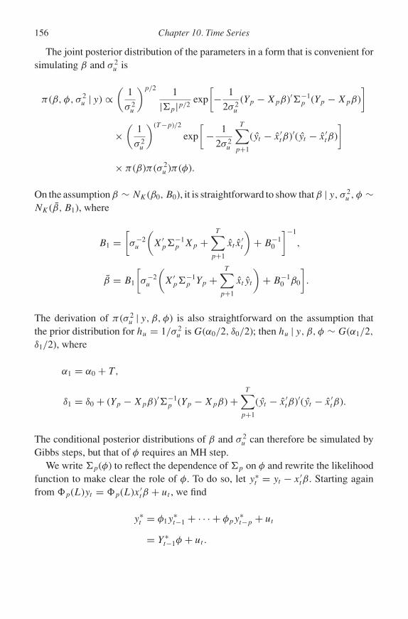
P1: KAE



The joint posterior distribution of the parameters in a form that is convenient forsimulating β and σ 2

u is

π (β, φ, σ 2u | y) ∝

(1

σ 2u

)p/2 1

|p|p/2exp

[− 1

2σ 2u

(Yp − Xpβ)′−1p (Yp − Xpβ)

]

×(

1

σ 2u

)(T −p)/2

exp

[− 1

2σ 2u

T∑p+1

(yt − x ′tβ)′(yt − x ′

tβ)

]× π (β)π (σ 2

u )π (φ).

On the assumption β ∼ NK (β0, B0), it is straightforward to show that β | y, σ 2u , φ ∼

NK (β, B1), where

B1 =[σ−2

u

(X′

p−1p Xp +

T∑p+1

xt x′t

)+ B−1

0

]−1

,

β = B1

[σ−2

u

(X′

p−1p Yp +

T∑p+1

xt yt

)+ B−1

0 β0

].

The derivation of π (σ 2u | y, β, φ) is also straightforward on the assumption that

the prior distribution for hu = 1/σ 2u is G(α0/2, δ0/2); then hu | y, β, φ ∼ G(α1/2,

δ1/2), where

α1 = α0 + T ,

δ1 = δ0 + (Yp − Xpβ)′−1p (Yp − Xpβ) +

T∑p+1

(yt − x ′tβ)′(yt − x ′

tβ).

The conditional posterior distributions of β and σ 2u can therefore be simulated by

Gibbs steps, but that of φ requires an MH step.We write p(φ) to reflect the dependence of p on φ and rewrite the likelihood

function to make clear the role of φ. To do so, let y∗t = yt − x ′

tβ. Starting againfrom �p(L)yt = �p(L)x ′

tβ + ut , we find

y∗t = φ1y

∗t−1 + · · · + φpy∗

t−p + ut

= Y ∗t−1φ + ut .

P1: KAE


10.1 Autoregressive Models 157

Accordingly, for t > p, y∗t ∼ N(Y ∗

t−1φ, σ 2). The conditional posterior distributionof φ is therefore

φ | y, β, σ 2u ∝ 1

|p(φ)|T/2exp

[− 1

2σ 2u

(Yp − Xpβ)′p(φ)−1(Yp − Xpβ)

]

× exp

− 1

2σ 2u

T∑p+1

(y∗t − Y ∗

t−1φ)′(y∗t − Y ∗

t−1φ)

×π (φ)1(φ ∈ Sφ), (10.4)

where Sφ is the region in which the process is stationary. This distribution is clearlynonstandard, but it can be sampled with an MH algorithm after specifying the priordistribution of φ; for example, φ ∼ Np(φ0, �0). A possible proposal generatingdensity is the distribution obtained by multiplying π (φ) by the terms involving y∗

t ,t > p, in (10.4); that distribution is N(φ, �), where

� =σ−2

u

T∑p+1

Y ∗′t−1Y

∗t−1 + �−1

0

−1

,

φ = �

σ−2u

T∑p+1

Y ∗′t−1y

∗t + �−1

0 φ0

.

Draws of φ from that distribution are made until one is found that is in the stationaryregion; it is then subjected to the usual MH acceptance criterion.

As an example, we examine the expectations augmented Phillips curve model aspresented in Wooldridge (2006, pp. 390–391). The data are monthly observations oninflation and the unemployment rate for the period 1948 January to 2005 November,and the model is

yt = x ′tβ + ut , (10.5)

ut = ρut−1 + εt , (10.6)

where εt ∼ N(0, σ 2), yt is the change in inflation rate, and xt includes a constantand the unemployment rate. We employ the training sample approach to specify hy-perparameters for the priors, where the training period is January 1948 to December1952. The hyperparameters are estimated from a regression of y on x that allowsfor first-order autocorrelated errors. We set α0 = 2.001 to allow for a large varianceand set B0 at the estimated variance from the training sample.

The results are shown in Table 10.1. The coefficient of unemployment, β2, isclearly negative; its 95% credibility interval is (−0.082, −0.036), and its meanof −0.059 is in the middle of the interval. The autocorrelation parameter φ isclearly positive. Its mean of 0.234, along with the fairly tight credibility interval,

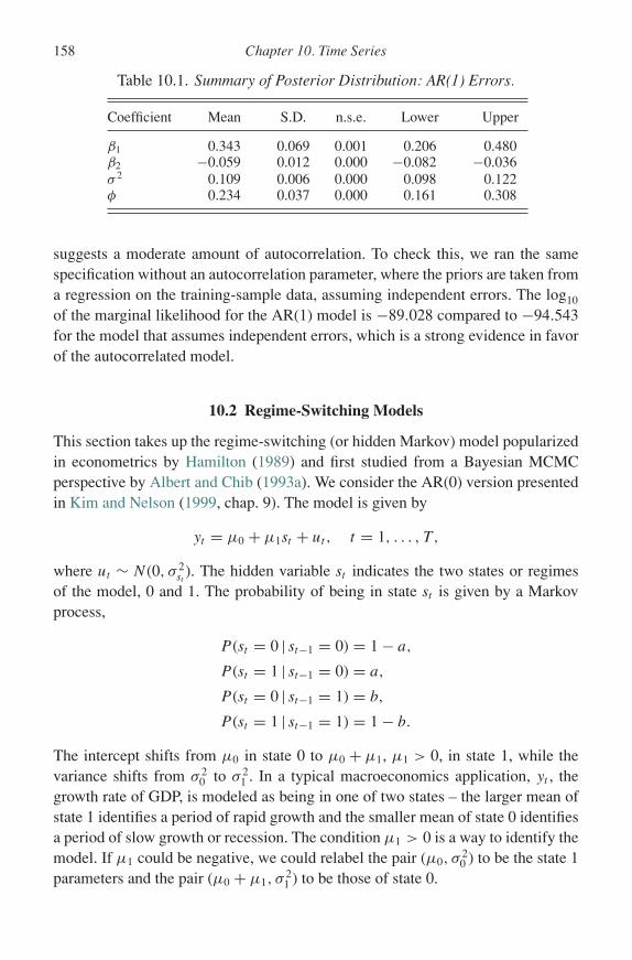
P1: KAE



Table 10.1. Summary of Posterior Distribution: AR(1) Errors.


β1 0.343 0.069 0.001 0.206 0.480β2 −0.059 0.012 0.000 −0.082 −0.036σ 2 0.109 0.006 0.000 0.098 0.122φ 0.234 0.037 0.000 0.161 0.308

suggests a moderate amount of autocorrelation. To check this, we ran the samespecification without an autocorrelation parameter, where the priors are taken froma regression on the training-sample data, assuming independent errors. The log10

of the marginal likelihood for the AR(1) model is −89.028 compared to −94.543for the model that assumes independent errors, which is a strong evidence in favorof the autocorrelated model.

10.2 Regime-Switching Models

This section takes up the regime-switching (or hidden Markov) model popularizedin econometrics by Hamilton (1989) and first studied from a Bayesian MCMCperspective by Albert and Chib (1993a). We consider the AR(0) version presentedin Kim and Nelson (1999, chap. 9). The model is given by

yt = µ0 + µ1st + ut , t = 1, . . . , T ,

where ut ∼ N(0, σ 2st

). The hidden variable st indicates the two states or regimesof the model, 0 and 1. The probability of being in state st is given by a Markovprocess,

P (st = 0 | st−1 = 0) = 1 − a,

P (st = 1 | st−1 = 0) = a,

P (st = 0 | st−1 = 1) = b,

P (st = 1 | st−1 = 1) = 1 − b.

The intercept shifts from µ0 in state 0 to µ0 + µ1, µ1 > 0, in state 1, while thevariance shifts from σ 2

0 to σ 21 . In a typical macroeconomics application, yt , the

growth rate of GDP, is modeled as being in one of two states – the larger mean ofstate 1 identifies a period of rapid growth and the smaller mean of state 0 identifiesa period of slow growth or recession. The condition µ1 > 0 is a way to identify themodel. If µ1 could be negative, we could relabel the pair (µ0, σ

20 ) to be the state 1

parameters and the pair (µ0 + µ1, σ21 ) to be those of state 0.

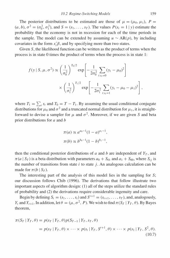
P1: KAE


10.2 Regime-Switching Models 159

The posterior distributions to be estimated are those of µ = (µ0, µ1), P =(a, b), σ 2 = (σ 2

0 , σ 21 ), and S = (s1, . . . , sT ). The values P (st = 1 | y) estimate the

probability that the economy is not in recession for each of the time periods inthe sample. The model can be extended by assuming u ∼ AR(p), by includingcovariates in the form x ′

tβ, and by specifying more than two states.Given S, the likelihood function can be written as the product of terms when the

process is in state 0 times the product of terms when the process is in state 1:

f (y | S, µ, σ 2) ∝(

1

σ 20

)T0/2

exp

[− 1

2σ 20

∑t :st=0

(yt − µ0)2

]

×(

1

σ 21

)T1/2

exp

[− 1

2σ 21

∑t :st=1

(yt − µ0 − µ1)2

],

where T1 = ∑t st and T0 = T − T1. By assuming the usual conditional conjugate

distributions for µ0 and σ 2 and a truncated normal distribution for µ1, it is straight-forward to devise a sampler for µ and σ 2. Moreover, if we are given S and betaprior distributions for a and b

π (a) ∝ aa0−1(1 − a)a1−1,

π (b) ∝ bb0−1(1 − b)b1−1,

then the conditional posterior distributions of a and b are independent of YT , andπ (a | ST ) is a beta distribution with parameters a0 + S01 and a1 + S00, where Sij isthe number of transitions from state i to state j . An analogous calculation can bemade for π (b | ST ).

The interesting part of the analysis of this model lies in the sampling for S;our discussion follows Chib (1996). The derivations that follow illustrate twoimportant aspects of algorithm design: (1) all of the steps utilize the standard rulesof probability and (2) the derivations require considerable ingenuity and care.

Begin by defining St = (s1, . . . , st ) and St+1 = (st+1, . . . , sT ), and, analogously,Yt and Yt+1. In addition, let θ = (µ, σ 2, P ). We wish to find π (ST |YT , θ ). By Bayestheorem,

π (ST | YT , θ ) = p(sT |YT , θ )p(ST −1 |YT , sT , θ )

= p(sT |YT , θ ) × · · · × p(st |YT , St+1, θ ) × · · · × p(s1 |YT , S2, θ ).(10.7)

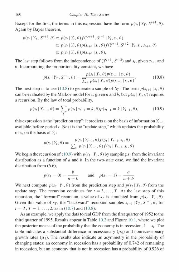
P1: KAE



Except for the first, the terms in this expression have the form p(st |YT , St+1, θ ).Again by Bayes theorem,

p(st | YT , St+1, θ ) ∝ p(st |Yt , θ )f (Y t+1, St+1 |Yt , st , θ )

∝ p(st |Yt , θ )p(st+1 | st , θ )f (Y t+1, St+2 |Yt , st , st+1, θ )

∝ p(st |Yt , θ )p(st+1 | st , θ ).

The last step follows from the independence of (Y t+1, St+2) and st , given st+1 andθ . Incorporating the proportionality constant, we have

p(st |YT , St+1, θ ) = p(st |Yt , θ )p(st+1 | st , θ )∑st

p(st |Yt , θ )p(st+1 | st , θ ). (10.8)

The next step is to use (10.8) to generate a sample of ST . The term p(st+1 | st , θ )can be evaluated by the Markov model for st given a and b, but p(st |Yt , θ ) requiresa recursion. By the law of total probability,

p(st | Yt−1, θ ) =∑

k

p(st | st−1 = k, θ )p(st−1 = k |Yt−1, θ ), (10.9)

this expression is the “prediction step”: it predicts st on the basis of information Yt−1

available before period t . Next is the “update step,” which updates the probabilityof st on the basis of Yt :

p(st |Yt , θ ) = p(st |Yt−1, θ )f (yt |Yt−1, st , θ )∑st

p(st |Yt−1, θ )f (yt |Yt−1, st , θ ).

We begin the recursion of (10.9) with p(s1 |Y0, θ ) by sampling s1 from the invariantdistribution as a function of a and b. In the two-state case, we find the invariantdistribution from (6.6),

p(s1 = 0) = b

a + band p(s1 = 1) = a

a + b.

We next compute p(s2 |Y1, θ ) from the prediction step and p(s2 |Y2, θ ) from theupdate step. The recursion continues for t = 3, . . . , T . At the last step of thisrecursion, the “forward” recursion, a value of sT is simulated from p(sT |YT , θ ).Given this value of sT , the “backward” recursion samples st−1 |YT , St+1, θ , fort = T , T − 1, . . . , 2, as in (10.7) and (10.8).

As an example, we apply the data to real GDP from the first quarter of 1952 to thethird quarter of 1995. Results appear in Table 10.2 and Figure 10.1, where we plotthe posterior means of the probability that the economy is in recession, 1 − st . Thetable indicates a substantial difference in recessionary (µ0) and nonrecessionarygrowth rates (µ1). The results also indicate an asymmetry in the probability ofchanging states: an economy in recession has a probability of 0.742 of remainingin recession, but an economy that is not in recession has a probability of 0.926 of

P1: KAE


10.3 Time-Varying Parameters 161

Table 10.2. Parameter Estimates for GDP Data.

Parameter Mean S. D. Median

µ0 −0.353 0.266 −0.339µ1 1.334 0.232 1.322σ 2 0.579 0.076 0.5721 − a 0.742 0.085 0.7511 − b 0.926 0.034 0.930

not going into recession. The figure suggests a fairly clear-cut distinction betweenrecessionary and nonrecessionary periods since only a few of the 175 observationsare around 0.5.

10.3 Time-Varying Parameters

The model discussed in this section assumes that regression coefficients evolve ran-domly through time. It is written in state–space form and consists of the observation

54 56 58 60 62 64 66 68 70 72 74 76 78 80 82 84 86 88 90 92 940

0.1

0.2

0.3

0.4

0.5

0.6

0.7

0.8

0.9

1

Figure 10.1. Probability of recession.

P1: KAE



equation

yt = x ′tβt + ut , (10.10)

and the transition equation

βt = βt−1 + εt , (10.11)

where t = 1, . . . , T , yt and ut are scalars, xt , βt , and εt are K × 1 vectors, ut ∼N(0, σ 2), and εt ∼ NK (0, ). We further assume that the ut and εt are independentof each other and through time. The initial state β0 can be given a fixed value or canbe assumed to have a normal distribution with known mean and variance. Anotherpossibility is to specify a hierarchical model for β0. For simplicity, we take β0 tobe a known vector. This model can be generalized to a vector autoregression byallowing yt to be a vector.

To analyze this model we define

Y = (yT , yT −1, . . . , y1)′,

β = (βT , βT −1, . . . , β1)′,

u = (uT , uT −1, . . . , u1),

ε = (εT , εT −1, . . . , ε1)′,

X =

x ′

T 0 0 0

0 x ′T −1 . . . 0

......

. . . 0

0 0 . . . x ′1

.

The likelihood function is

f (y | β, σ 2) ∝(

1

σ 2

)T/2

exp

[− 1

2σ 2(y − Xβ)′(y − Xβ)

].

The transition equation leads to a prior distribution for β: by defining the KT × KT

matrix H

H =

IK −IK 0 . . . 0

0 IK −IK . . . 0... 0 IK

. . . 0... 0

. . . . . . 0

0 0 0 0 IK

,

P1: KAE


10.3 Time-Varying Parameters 163

we can write Hβ = β0 + ε, where β0 is a TK × 1 vector with β0 in the last K rowsand zeros elsewhere. It follows that β = H−1β0 + H−1ε, from which we concludethat

β ∼ NK (H−1β0, H−1(IT ⊗ )(H−1)′).

We adopt standard priors for the remaining parameters: 1/σ 2 ∼ G(α0/2, δ0/2) and−1 ∼ WK (ν0, S0). The joint posterior distribution is

π (β, σ 2, | y) ∝(

1

σ 2

)T/2

exp

[− 1

2σ 2(y − Xβ)′(y − Xβ)

]1

||T/2

× exp

[− 1

2(β − H−1β0)′H ′(IT ⊗ −1)H (β − H−1β0)

]

×(

1

σ 2

)α0/2−1

exp

[− δ0

2σ 2

]1

||(ν0−K−1)/2exp

[− 1

2tr(S−1

0 −1)

],

where we have used |H ′(IT ⊗ −1)H | = |H ′||IT ⊗ −1||H |, |H | = 1, and(A.20).

A Gibbs algorithm can be used because the conditional posterior distributionsare available for sampling:

β|y, σ 2, ∼ NT K (β, B1),

(1/σ 2)|y, β, ∼ G(ν1/2, δ1/2),

−1 ∼ WK (ν1, S1),

where

B1 = [(1/σ 2)X′X + H ′(IT ⊗ −1)H

]−1,

β = B1[(1/σ 2)X′y + H ′(IT ⊗ −1)β0

],

α1 = α0 + T ,

δ1 = δ0 + (y − Xβ)′(y − Xβ),

ν1 = ν0 + T ,

S1 =[S−1

0 +T∑

t=1

(βt − βt−1)(βt − βt−1)′]−1

.

P1: KAE



The expression for S1 follows from

(β − H−1β0)′H ′(IT ⊗ −1)H (β − H−1β0) = (Hβ − β0)′(I ⊗ −1)(Hβ − β0)

=

βT − βT −1...

β1 − β0

′

−1 0 0 00 −1 0 0...

. . ....

0 0 0 −1

βT − βT −1

...β1 − β0

=T∑

t=1

(βt − βt−1)′−1(βt − βt−1)

= tr

[T∑

t=1

(βt − βt−1)(βt − βt−1)′−1

].

This algorithm must be modified for large KT because B1 is the inverse of aKT × KT matrix that may be too large to invert rapidly and accurately. The matrixinversion can be avoided by sampling βt with the same type of recursive schemeutilized in sampling for st in Section 10.2.

As an example of this model, we return to the Phillips curve model discussedin Section 10.1, but we now assume that βt follows a random walk, rather thanbeing constant, and that ut is not autocorrelated. The model is that of Equations(10.10) and (10.11), where yt is the change in the inflation rate and xt consists ofa constant and the unemployment rate. The priors are again based on the first 5years of data employed as a training sample, and βt is taken as a constant over thetraining sample to specify the hyperparameters.

Table 10.3 and Figure 10.2 contain results, where the lower and upper limitsrefer to a 90% credibility interval. Results are based on 20,000 draws from theposterior distribution after 1,000 burn-in iterations. The log10 marginal likelihoodvalue is −92.506. The AR(1) model has a larger marginal likelihood despite thelarge variation in the values of βt displayed in Figure 10.2.

Table 10.3. Summary of Posterior Distribution: Time VaryingParameter Model.

Coefficient Mean S.D. Lower Upper

σ11 0.006 0.003 0.003 0.010σ12 −0.001 0.001 −0.002 −0.001σ22 0.000 0.000 0.000 0.000σ 2 0.103 0.006 0.096 0.111

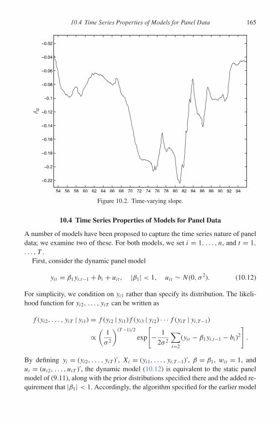
P1: KAE


10.4 Time Series Properties of Models for Panel Data 165

54 56 58 60 62 64 66 68 70 72 74 76 78 80 82 84 86 88 90 92 94

2

1

β t2

Figure 10.2. Time-varying slope.

10.4 Time Series Properties of Models for Panel Data

A number of models have been proposed to capture the time series nature of paneldata; we examine two of these. For both models, we set i = 1, . . . , n, and t = 1,

. . . , T .First, consider the dynamic panel model

yit = β1yi,t−1 + bi + uit , |β1| < 1, uit ∼ N(0, σ 2). (10.12)

For simplicity, we condition on yi1 rather than specify its distribution. The likeli-hood function for yi2, . . . , yiT can be written as

f (yi2, . . . , yiT | yi1) = f (yi2 | yi1)f (yi3 | yi2) · · · f (yiT | yi,T −1)

∝(

1

σ 2

)(T −1)/2

exp

[− 1

2σ 2

∑t=2

(yit − β1yi,t−1 − bi)2

].

By defining yi = (yi2, . . . , yiT )′, Xi = (yi1, . . . , yi,T −1)′, β = β1, wit = 1, andui = (ui2, . . . , uiT )′, the dynamic model (10.12) is equivalent to the static panelmodel of (9.11), along with the prior distributions specified there and the added re-quirement that |β1| < 1. Accordingly, the algorithm specified for the earlier model

P1: KAE



is applicable, except that the sampling for β1 is from a normal distribution truncatedto (−1, 1).

Second, consider a model that includes unit-specific regression coefficients andan AR(1) disturbance term:

yit = x ′itβ + w′

it bi + εit , εit = ρεi,t−1 + uit , |ρ| < 1, (10.13)

where uit ∼ N(0, σ 2) independent over i and t . A standard analysis shows that

Cov(εit , εi,t−s) = σ 2

1 − ρ2ρs,

which implies that yi |β, bi, ρ, σ 2 ∼ N(Xiβ + Wibi,σ 2

1−ρ2 �), where

� =

1 ρ ρ2 . . . ρT −1

ρ 1 ρ . . . ρT −2

......

... . . ....

ρT −1 ρT −2 . . . ρ 1

.

We may again utilize the specification in (9.11) by adding a prior distributionfor ρ, say ρ ∼ TN(−1,1)(ρ0, R0), and modifying the likelihood function to

f (y | β, b, σ 2, ρ) ∝(

σ 2

1 − ρ2

)−T/21

|�|T/2

× exp

[−1 − ρ2

2σ 2

∑i

(yi −Xiβ−Wibi)′�−1(yi −Xiβ−Wibi)

].

We leave the details of the algorithm as an exercise.


Chapter 10 Useful sources for time series, primarily from the frequentist view-point, are Hamilton (1994) and Harvey (1989). Such standard texts as Greene(2003, chaps. 12, 20) also cover the basic ideas.

Secton 10.1 Chib (1993) considers the AR(p) model conditioned on the first p

observations in which case all the updates are in closed form and no MH step isrequired. The general ARMA(p, q) model without conditioning is covered fromthe Bayesian viewpoint in Chib and Greenberg (1994). The Phillips curve examplewas estimated with the “AR” model in the BACC program. See Geweke (2005,sec. 7.1) for details.

P1: KAE


10.6 Exercises 167

Section 10.2 State–space models are discussed from a Bayesian viewpoint byCarlin et al. (1992b), Carter and Kohn (1994), Fruhwirth-Schnatter (1994), de Jongand Shephard (1995), Chib and Greenberg (1995a), and Kim and Nelson (1999);the latter provide downloadable Gauss software. The results contained in the textwere computed with their program GIBS MS0.PRG. Further discussion of thehidden Markov model from the Bayesian viewpoint may be found in Chib (2001,sec. 8.8), which builds on Albert and Chib (1993a) and Chib (1996).

The regime-switching model is a mixture model,

yt ∼ P (st = 0)N(µ0, σ20 ) + P (st = 1)N(µ0 + µ1, σ

21 ).

As noted before, this model is not identified without a restriction such as µ1 > 0,because the state labels and all parameters could be switched. The restriction hasthe effect of forcing the mean of the distribution in state 1 to be greater than themean in state 0. Without such a restriction, the sampler would generate a bimodaldistribution for the means and variances. More generally, the question of howto deal with label switching has been studied extensively. While the solution wehave adopted works well in the regime-switching model, the question of how todeal with models with more states and more parameters is not settled. For anintroduction, suggested solutions, and further references, see Celeux et al. (2000)and Fruhwirth-Schnatter (2001).

Section 10.3 More details and references to an MCMC algorithm for this model isin Chib (2001, sec. 8.9); a discussion and downloadable programs are in Kim andNelson (1999, chap. 9). A model that combines regime switching and time-varyingparameters, along with downloadable programs, is described in Kim and Nelson(1999, chap. 10).

Section 10.4 The panel data model with correlated errors is discussed in Chib(in press-b).

10.6 Exercises

10.1 Verify that the state–space form (10.3) reproduces the AR(p) model of (10.1).10.2 Explain how to find the predictive distribution for yT +1 if yt ∼ AR(p), given a sample

of draws from the posterior distributions of β, φ, and σ 2u .

10.3 Provide the details of an algorithm to analyze the model of (10.13).10.4 Modify the SUR model to include first-order autocorrelation, and describe an algo-

rithm for estimating parameters.

P1: KAE


Chapter 11

Endogenous Covariates and Sample Selection

THIS CHAPTER IS CONCERNED with data sets for which the assumption madeabout the exogeneity of covariates in Chapter 4 and subsequent chapters is unten-able. Covariates that are correlated with the disturbance term are called endogenousvariables in the econometrics literature. We take up three types of models in whichendogeneity may be present: treatment models, unobserved covariates, and sampleselection subject to incidental truncation.

11.1 Treatment Models

Treatment models are used to compare responses of individuals who belong eitherto a treatment or a control group. If the assignment to a group is random, as inmany of the clinical trials that arise in biostatistical applications, the assignmentmay be regarded as independent of any characteristics of the individual. But inmany economic applications and in clinical trials in which compliance is notguaranteed, whether an individual is in the treatment or control group may dependon unobserved covariates that are correlated with the response variable. Suchunobserved covariates are called confounders in the statistical literature; in theeconometrics literature, the treatment assignment is called endogenous when it isnot independent of the response variable. As an example, let the response variable bewages and the treatment be participation in a job training program. We might expectthat people with sufficient motivation to participate in training would earn higherwages, even without participating in the program, than those with less motivation.The problem may be less serious if individuals are randomly assigned to the trainingprogram, but there may still be confounding. For example, individuals assignedto the program may choose not to participate, and individuals not assigned to theprogram may find a way to participate. Inferences drawn from models that ignoreconfounding may yield misleading results.

168

P1: KAE


11.1 Treatment Models 169

To model this situation, we suppose that the response variable is related to thecovariates and the treatment assignment through

y0i = x ′iβ0 + u0i ,

y1i = x ′iβ1 + u1i ,

(11.1)

where xi is a K1 vector of covariates, a 0 subscript indicates assignment to the con-trol group, and 1 indicates assignment to the treatment group. The group assignmentis determined by the binary variable si ,

si ={

0, if i is assigned to control group,

1, if i is assigned to treatment group.

An important objective of such studies is to determine the effect of the treatmenton the response. The average treatment effect is a measure of this effect; it is definedas

ATE = E(y1i − y0i |xi) = x ′i(β1 − β0).

Because an individual is assigned to either the treatment or control group, how-ever, only one of y0i and y1i are observed. In the presence of confounding, thedata provide information about E(y1i |si = 1) and E(y0i |si = 0), but the differencebetween these is not the ATE, because of the correlation between y0i and si andbetween y1i and si :

E(y1i |si = 1) − E(y0i |si = 0) = x ′i(β1 − β0) + [E(u1i |si = 1) − E(u0i |si = 0)],

and the bracketed term is not equal to zero in the presence of confounding.One approach to solving the problem caused by confounders is to model the

assignment decision. We consider a method that uses one or more instrumentalvariables (IVs). These are variables that have two properties:

11.1 They are independent of u0i and u1i .11.2 They are not independent of si .

In the wage–job training program example, a possible IV is the score on an intelli-gence test: we would not expect the test score itself to affect wages, and we wouldnot expect the decision to participate to be independent of intelligence. By their in-dependence from the confounders, the IVs introduce an element of randomizationinto data that were not generated by random assignment. In particular, we assume

s∗i = x ′

iγ1 + z′iγ2 + vi,

si ={

1, if s∗i > 0,

0, if s∗i ≤ 0,

(11.2)

P1: KAE


170 Chapter 11. Endogenous Covariates and Sample Selection

and set

yi = (1 − si)y0i + siy1i , (11.3)

where zi is a K2 × 1 vector of instrumental variables. The latent data value s∗i

for the treatment indicator si is modeled as a binary probit variable. Confoundingor endogeneity appears in this model if there is a correlation between u0i and vi

and between u1i and vi . We regard the correlation as arising from an unobservedcovariate that affects both the observed response yi and whether or not i receivesthe treatment. The covariance matrices are

Cov(u0i , vi) ≡ 0 =(

σ00 σ0v

σ0v 1

), Cov(u1i , vi) ≡ 1 =

(σ11 σ1v

σ1v 1

),

where σvv = 1 because of the probit specification.We now develop a Gibbs algorithm to draw a sample from the posterior distri-

bution of the parameters. First, some definitions and notation. For the remainder ofthe section, j = 0, 1 indicates the untreated and treated groups, respectively. Letβ = (β ′

0, β′1, γ

′1, γ

′2)′, γ = (γ ′

1, γ′2)′,

Xji =(

(1 − j )x ′i jx ′

i 0 00 0 x ′

i z′i

),

y, X, Z, respectively, are the observations on yi , xi , and zi , s∗ represents the la-tent data s∗

i , N0 = {i : si = 0}, N1 = {i : si = 1}, and n0 and n1, respectively, arethe number of observations in N0 and N1. We assume a Gaussian prior distribu-tion for β ∼ Np(b0, B0), where p = 3K1 + K2. To expedite the simulation, wereparameterize the variances in j as ωjj = σjj − σ 2

jv, which is positive becauseωjj = |j | and j is positive definite. We define ψj = (ωjj , σjv) and specify theprior distributions

π (ψj ) = π (ωjj )π (σjv|ωjj )

= IG(νj0/2, dj0/2)N (mj0, ωjjMj0).

The posterior distribution has the form

π (β,ψ0, ψ1, s∗|y, s) = π (β)π (ψ0)π (ψ1)

∏i

[[1(si = 0)1(s∗i ≤ 0) + 1(si = 1)

× 1(s∗i > 0)]N2(yi, s

∗i |X0iβ,0))1−si (N2(yi, s

∗i |X1iβ,1))si ],

and the Gibbs algorithm proceeds in four blocks: ψ0, ψ1, β, and s∗.The ψj blocks may be sampled by the method of composition,

π (ψj |β, s∗, y, X, Z) = π (σjv|ωjj , β, s∗, y, X, Z)π (ωjj |β, s∗, y, X, Z).

P1: KAE


11.1 Treatment Models 171

For the first of these, you will be asked to show in Exercise 11.1 that

yji |s∗i , βj , γ, ψj ∼ N(x ′

iβj + σjvei, ωjj ), (11.4)

where ei = s∗i − x ′

iγ1 − z′iγ2. Let Yj , Xj , Zj , S∗

j , and Ej , respectively, contain thevalues of yji , xi , zi , s∗

i , and ei for i ∈ Nj . Then

Yj |S∗j , βj , γ, ψj ∼ Nnj

(Xjβj + σjvEj , ωjj Inj

). (11.5)

Because σjv appears in (11.5) as a regression parameter, its conditional posteriordistribution is easily obtained. The next step is to obtain the conditional posteriordistribution of ωjj after marginalizing out σjv with respect to its prior distribution.From (11.5), you will verify in Exercise 11.2 that

E(Yj |S∗j , βj , γ, ωjj ) = Xjβj + mj0Ej , (11.6)

Var(Yj |S∗j , γ, ωjj ) = ωjj

(Inj

+ EjMj0E′j

). (11.7)

Equation (11.5) is multiplied by the prior distribution of ωjj to obtain its conditionalposterior distribution, which has the form of an inverse gamma distribution.

In the second block, we sample for β conditioned on all other parameters and thedata. This step uses the SUR setup of Section 9.1. In the third block, s∗ is sampledfrom the usual truncated normal distributions. You are asked to supply the detailsof the distributions in Exercise 11.4.


Algorithm 11.1: Gibbs algorithm for treatment model (Chib, in press-a)

11.1 Sample ψj conditioned on (y, s∗, X,Z, β)(a) Drawing ωjj marginalized over σjv from

IG

(νj0 + nj

2,dj0 + dj

2

),

where

dj = (Yj − Xjβj − mj0Ej )′(Inj

+ EjMj0E′j

)−1(Yj − Xjβj − mj0Ej ),

(b) Drawing σjv conditioned on ωjj from N (cj , ωjjCj ), where

cj = Cj

[M−1

j0 mj0 + E′j (Yj − Xjβj )

],

Cj = (M−1

j0 + E′jEj

)−1.

11.2 Sample β conditioned on (y, s∗, ψ0, ψ1) from Np(β, B), where

β = B

(B−1

0 b0 +∑i∈N0

X′0i

−10 y∗

i +∑i∈N1

X′1i

−11 y∗

i

),

B =(

B−10 +

∑i∈N0

X′0i

−10 X0i +

∑i∈N1

X′1i

−11 X1i

)−1

,

P1: KAE



and y∗i = (yi, s

∗i )′.

11.3 Sample s∗ conditioned on (y,X,Z, β,ψ0, ψ1) by drawing

s∗i from

{TN(−∞,0)

(µ0i , φ

20

), if si = 0,

TN(0,∞)(µ1i , φ

21

), if si = 1,

where

µji = x ′iγ1 + z′

iγ2 + σjvσ−1jj (yji − x ′

iβj ),

φ2j = 1 − σ 2

jvσ−1jj .

We compute the marginal likelihood for this model by the Chib method ofSection 7.1.2; it uses the fact that the log of the marginal likelihood m(y, s|X, Z)can be written as

log m(y, s|X,Z) = log f (y, s|X,Z, β∗, ψ∗0 , ψ∗

1 ) + log π (β∗, ψ∗0 , ψ∗

1 )

− log π (β∗, ψ∗0 , ψ∗

1 |y, s,X,Z),

where (β∗, ψ∗0 , ψ∗

1 ) is, say, the posterior mean of the parameters from the MCMCrun, the first term is the log likelihood, the second is the log prior, and the third isthe log posterior, and all are evaluated at (β∗, ψ∗

0 , ψ∗1 ). The second term is available

directly. The first term is∑i∈N0

log f (y0i , si = 0|xi, zi, β∗, ψ∗

0 ) +∑i∈N1

log f (y1i , si = 1|xi, zi, β∗, ψ∗

1 ).

For j = 0, we have

f (y0i , si = 0|xi, zi, β, ψ0) = f (y0i |xi, zi, β, ψ0)∫ 0

−∞f (s∗

i |y0i , xi, zi, β, ψ0) ds∗i

= N (y0i |x ′iβ0, σ00)�

(−µ0i

φ0

).

A similar analysis for j = 1 (see Exercise 11.3), shows that both cases can bewritten as

f (yji, si = j |xi, zi, β, ψj ) = N(yji |x ′iβj , σjj )�

((2j − 1)

µji

φj

). (11.8)

The third term can be estimated by decomposing it as

π (β∗, ψ∗0 , ψ∗

1 |y, s, X, Z) = π (ψ∗0 , ψ∗

1 |y, s, X, Z)π (β∗|y, s, X, Z, ψ∗0 , ψ∗

1 ),

from which π (ψ∗0 , ψ∗

1 |y, s, X, Z) is obtained by averaging the product of theinverse gamma and normal densities in step 1 of Algorithm 11.1 over the MCMCdraws and π (β∗|y, s, X, Z, ψ∗

0 , ψ∗1 ) is obtained by fixing (ψ0, ψ1) at (ψ∗

0 , ψ∗1 ),

running the MCMC algorithm with the remaining unknowns, and averaging thenormal density in step 2 over the resulting draws.

P1: KAE


11.2 Endogenous Covariates 173

11.2 Endogenous Covariates

In the econometrics literature, the endogenous covariate is often continuous, ratherthan binary as in the treatment variables discussed in the previous section. Weexamine a simple example to understand the nature of the problems caused by thepresence of endogenous covariates. Let

yi = x ′iβ1 + βsxis + ui, i = 1, . . . , n,

and suppose that the K1 covariates in xi are independent of ui , but that ui and xis

have a joint normal distribution,(ui

xis

)∼ N2

((0

E(xis)

),

(σ11 σ12

σ12 σ22

)),

where σ12 = 0. Equation (A.9) implies that the distribution of yi |xi, xis is Gaussianwith parameters

E(yi |xi, xis) = x ′iβ1 − σ12

σ22E(xis) +

(βs + σ12

σ22

)xis,

Var(yi) = σ11 − σ 212

σ22.

This result has an important implication. Since ∂E(yi )∂xis

= βs + σ12σ22

, the likelihoodfunction contains information about βs + σ12

σ22, not βs ; equivalently, in the absence

of observations on ui , βs is not identifiable. We have no way of separating βs fromβs + σ12

σ22.

As an example of how this situation may arise, let yi be the hourly wage ofindividual i, xi be a vector of covariates that control for demographic and economicfactors, and xis be i’s years of schooling. Let us assume that an unobserved variable,call it intelligence, affects both wages and schooling; that is, an individual withhigher intelligence would tend to earn a higher wage for any level of schoolingand attain a higher level of education (σ12 > 0) than an individual with lowerintelligence. In that case, the coefficient on education measures both the directeffect of schooling through βs and the indirect effect through the relationshipbetween schooling and intelligence σ12

σ22.

If the relation between education and intelligence is ignored, the effect of edu-cation on wages of schooling is overestimated by σ12

σ22. This may be important for

public policy. Suppose it is decided to choose people randomly from the populationto receive an additional year of schooling. Being chosen randomly, some of thepeople receiving the additional year will be of lower intelligence levels than thosein the first sample who made their schooling decisions without the policy inter-vention. The increase in wages for the group will be closer to βs than to βs + σ12

σ22,

P1: KAE



and the policy may appear to be unsuccessful. It is thus important to find a way toestimate βs more accurately.

As was done before, we employ IVs to model the endogenous variable xis .Consider the system

yi = x ′iβ1 + βsxis + ui, (11.9)

xis = x ′iγ1 + z′

iγ2 + vi, (11.10)

where the K2 covariates in zi are the instrumental variables, assumed to be ex-ogenous to the system in the sense that they are independent of ui and vi .On the assumption that (ui, vi) ∼ N2(0, ), where = {σij }, this system, con-ditional on xi and zi , reproduces the correlation between ui and xis specifiedbefore.

The next step is to devise an MCMC algorithm to sample the parameters β =(β ′

1, βs)′, γ = (γ ′1, γ

′2)′, and . We begin with the latter and adopt a Wishart prior

for −1 ∼ W2(ν0, R0). Since (ui, vi) ∼ N2(0, ), we may write

π (|β, γ, y) ∝ ||−n/2 exp

[−1

2

∑(yi − X′

iβ, xis − Z′iγ )−1

(yi − X′

iβ

xis − Z′iγ

)]×||−(v0−3)/2 exp

[−1

2tr(R−1

0 −1)]

,

whereX′i = (x ′

i , xis) and Z′i = (x ′

i , z′i).

To sample β, we use f (yi, xis |θ ) = f (xis |θ )f (yi |xis, θ ), where θ = (β, γ, ),and specify a Gaussian prior NK1+1(β0, B0). By the properties of conditional dis-tributions of normal distributions, we have

yi |xis, θ ∼ N

(X′

iβ + σ12

σ22(xis − Z′

iγ ), ω11

),

where ω11 = σ11 − σ 212/σ22. From these considerations, we may write

π (β|γ,, y) ∝ exp

[− 1

2ω11

∑(yi − σ12

σ22(xis − Z′

iγ ) − X′iβ

)2]

× exp

[−1

2(β − β0)′B−1

0 (β − β0)

].

To obtain the posterior distribution for γ , we make use of the decompositionf (yi, xis |θ ) = f (yi |θ )f (xis |yi, θ ) and note that γ appears only in the second ex-pression. The standard results for conditional distributions of joint normal distri-butions yield

xis |yi, θ ∼ N

(Z′

iγ + σ12

σ11(yi − X′

iβ), ω22

),

P1: KAE


11.3 Incidental Truncation 175

where ω22 = σ22 − σ 212/σ11. We specify a Gaussian prior NK1+K2 (γ0, G0) and

obtain

π (γ |β,, y) ∝ exp

[− 1

2ω22

∑(xis − σ12

σ11(yi − X′

iβ) − Z′iγ

)2]

× exp

[−1

2(γ − γ0)′G−1

0 (γ − γ0)

].

It is now straightforward to derive the conditional posterior distributions forspecifying a Gibbs algorithm:

∼ W2(ν1, R1),

β ∼ N (β, B1),

γ ∼ N (γ , G1),

whereν1 =ν0 + n,

R1 =[R−1

0 +∑(

yi − X′iβ

xis − Z′iγ

)(yi − X′

iβ, xis − Z′iγ )

]−1

,

B1 =[B−1

0 + ω−111

∑XiX

′i

]−1

,

β =B1

(B−1

0 β0 + ω−111

∑Xi

[yi − σ12

σ22(xis − Z′

iγ )

]),

G1 =[G−1

0 + ω−122

∑ZiZ

′i

]−1

,

γ =G1

(G−1

0 γ0 + ω−122

∑Zi

[xis − σ12

σ11(yi − X′

iβ)

]).

11.3 Incidental Truncation

Incidental truncation arises when the response variable yi is not observed for allunits, and whether it is observed depends on the value of a “selection” variable si .Part or all of the covariate data xi are observed for all sample units. A well-knownexample of this situation is a model designed to explain the wage rate of marriedwomen on the basis of demographic and economic variables, where no wage rateis observed for women who do not work in the time period of observation, but partor all of the demographic and economic variables may be observed. The factorsdetermining the decision to work, which is the binary variable si = 1 if individual i

works and 0 otherwise, may not be independent of the wage rate, so that includingin the sample only those women who work is likely to result in a poor estimate ofthe effects of the covariates of interest. As another example, si may be a Tobit-typevariable rather than a binary variable, where yi is observed when si > 0. In the

P1: KAE



wage rate example, si may be the hours worked, which is bounded below at zero,rather than a binary variable for labor force participation. In other cases, yi may bea binary variable. For continuous yi , we assume

yi = x ′iβ1 + ui,

where xi is a K1 vector observed for all i, and yi is not observed if si = 0 and isobserved if si = 1. For the units that are observed,

E(yi |xi, si = 1) = x ′iβ1 + E(ui |xi, si = 1).

The last term on the right may not equal zero, because of correlation between ui andsi , and a model based on the specification of a zero expected value is misspecified.

To deal with sample selection, we assume that we have K2 instrumental variablescontained in the vector zi and that zi and xi are observed for all units. The modelis specified by

yi = x ′iβ1 + ui,

s∗i = x ′

iγ1 + z′iγ2 + vi,

si ={

0, if s∗i ≤ 0,

1, if si > 0,

where (ui, vi) ∼ N2(0, ) and

=(

σ11 σ12

σ12 1

).

The restriction σ22 = 1 arises from the binary probit model for si ; see Section 8.2.2.Letting N0 = {i : si = 0}, N1 = {i : si = 1}, and θ denote the parameters of the

model, we can write the contribution of i ∈ N0 to the posterior distribution as

π (s∗i , θ |si = 0)∝P (si = 0|s∗

i , θ )π (s∗i |θ )π (θ )

∝1(si = 0)1(s∗i ≤ 0)π (s∗

i |θ )π (θ ),

and of i ∈ N1,

π (s∗i , θ |si = 1, yi)∝f (si = 1, yi |θ, s∗

i )π (s∗i |θ )π (θ )

∝f (si = 1, yi, s∗i |θ )π (θ )

∝f (yi, s∗i |θ )P (si = 1|s∗

i , yi, θ )π (θ )

∝f (yi, s∗i |θ )1(si = 1)1(s∗

i > 0)π (θ ).

The posterior distribution is therefore

π (s∗, θ |s, y)∝π (θ )∏i∈N0

π (s∗i |θ )1(si = 0)1(s∗

i ≤ 0)

×∏i∈N1

f (yi, s∗i |θ )1(si = 1)1(s∗

i > 0). (11.11)

P1: KAE


11.3 Incidental Truncation 177

We begin the development of an MCMC algorithm to approximate the posteriordistribution by deriving the conditional posterior distribution of β = (β ′

1, γ′1, γ

′2)′.

Defining

ηi ={

(0, s∗i )′, i ∈ N0,

(yi, s∗i )′, i ∈ N1,

Xi =(

x ′i 0 0

0 x ′i z′

i

), J =

(0 00 1

),

we may write the likelihood terms involving β in SUR form as

π (β|y, s∗, ) ∝ exp

[− 1

2

∑i∈N0

(ηi − Xiβ)′J ′J (ηi − Xiβ)

]

× exp

[− 1

2

∑i∈N1

(ηi − Xiβ)′−1(ηi − Xiβ)

].

Note that the first row of ηi − Xiβ is zero after premultiplication by J . With theprior distribution β ∼ NK1+K2 (β0, B0), we have

β|y, s∗, ∼ NK1+K2 (β, B1),

where

B1 =[∑

i∈N0

X′iJXi +

∑i∈N1

X′i

−1Xi + B−10

]−1

,

β = B1

[∑i∈N0

X′iJ ηi +

∑i∈N1

X′i

−1ηi + B−10 β0

],

and we have used J ′J = J .We next turn to the sampling of the covariance matrix parameters σ12 and ω11 =

σ11 − σ 212, which appear in the likelihood function only for i ∈ N1. Sampling for ω11

is restricted to positive values and automatically yields a positive σ11 = ω11 + σ 212.

We assume the prior distribution ω−111 ∼ G(α0/2, δ0/2) and write f (yi, s

∗i |θ ) =

f (yi |s∗i , θ )f (s∗

i |θ ) to find

π (ω11|y, β, σ12) ∝(

1

ω11

)n1/2

exp

[− 1

2ω11

∑i∈N1

[yi − x ′iβ1 − σ12(s∗

i − x ′iγ1 − z′

iγ2)]2

]

×(

1

ω11

)α0/2−1

exp

[− δ0

2ω11

],

since ω11 does not appear in f (s∗i |θ ). This implies ω−1

11 |y, β, σ12 ∼ G(α1/2, δ1/2),where

α1 = α0 + n1,

δ1 = δ0 +∑i∈N1

[yi − x ′iβ1 − σ12(s∗

i − x ′iγ1 − z′

iγ2)]2.

P1: KAE



To sample σ12|y, β, ω11 we assume the prior distribution σ12 ∼ N(s0, S0) andfind

π (σ12|y, β, ω11) ∝ exp

[− 1

2ω11

∑i∈N1

[yi − x ′iβ1 − σ12(s∗

i − x ′iγ1 − z′

iγ2)]2

]

× exp

[− 1

2S0(σ12 − s0)2

],

which implies σ12|y, β, ω11 ∼ N(s, S), where

S =[ω−1

11

∑(s∗

i − x ′iγ1 − z′

iγ2)2 + S−10

]−1,

s = S[ω−1

11

∑(s∗

i − x ′iγ1 − z′

iγ2)(yi − x ′iβ1) + S−1

0 s0

].

To sample the s∗i , use (11.11) and write, for i ∈ N1,∏

i∈N1

f (yi, s∗i |θ )1(si = 1)1(s∗

i > 0) =∏i∈N1

f (s∗i |yi, θ )f (yi |θ )1(si = 1)1(s∗

i > 0),

which implies that the s∗i are drawn from truncated normal distributions:

s∗i ∼

TN(−∞,0](x ′

iγ1 + z′iγ2, 1), for i ∈ N0,

TN(0,∞)

(x ′

iγ1 + z′iγ2 + σ12

ω11 + σ 212

(yi − x ′iβ1),

ω11

ω11 + σ 212

), for i ∈ N1.

Although the sampler generates values of the latent data s∗i , it does not generate

values of the “missing” yi for i ∈ N0.As an example, we utilize the Mroz data described in Section 8.2.1. In this

example, we treat hours of work as a binary variable for whether an individual is in(si = 1) or out (si = 0) of the labor force. The response variable yi is log(wage),which is observed only for employed women. We follow the specification ofWooldridge (2002, pp. 468, 565) in setting

x ′ = (constant, educ, experience, experience squared),

z′ = (nwifeinc, age, childlt6, childge6),

where educ is the wife’s education and nwifeinc is household income other thanthat earned by the wife.

Except for the constant terms in β we set prior means of 0 and variances of1 in the belief that the effect of each of these variables on log(wages) would befairly small and knowing that the mean log wage for the sample is slightly largerthan 1. We set a 0 mean and variance of 10 for the constant terms because ofgreater uncertainty. The variance of log(wages) in the sample is slightly over 0.5,suggesting that σ11 = ω11 + σ 2

12 is of order of magnitude 1, which we split betweenthe two components equally to obtain a value of 0.5 for ω11. With a gamma prior

P1: KAE



Table 11.1. Summary of Posterior Distribution: Probit SelectionModel, Mroz Data.

Coefficient Mean SD Lower Upper Corr time

β11 −0.529 0.263 −1.035 −0.004 7.357β12 0.108 0.015 0.078 0.137 2.389β13 0.042 0.015 0.012 0.071 4.512β14 −0.001 0.000 −0.002 0.000 2.955γ11 0.226 0.502 −0.756 1.207 2.990γ12 0.132 0.025 0.083 0.181 3.154γ13 0.124 0.019 0.087 0.161 3.202γ14 −0.002 0.001 −0.003 −0.001 3.042γ21 −0.012 0.005 −0.022 −0.002 3.566γ22 −0.052 0.008 −0.069 −0.036 3.437γ23 −0.856 0.119 −1.090 −0.626 3.419γ24 0.037 0.043 −0.048 0.122 3.186ω11 0.444 0.031 0.386 0.507 1.514σ11 0.454 0.032 0.396 0.520 1.406ρ12 0.009 0.147 −0.292 0.279 14.353

distribution on 1/ω11 ≈ 2, from (A.1) we have E(1/ω11) = 2.0 = α/δ, and a smallvalue of δ is associated with a larger variance. Accordingly, we set δ = 2, or δ0 = 4to obtain a large variance and α = 4, or α0 = 8 to obtain the desired mean. Weassumed σ12 ∼ N(0, 1) to take a neutral stance on its sign and to set a fairly largevariance. For the simulation, we set a burn-in of 10,000 and keep 40,000 generatedvalues. A large number of iterations is chosen because of the complexity of themodel.

Summary results are in Table 11.1, and Figure 11.1 displays histograms of thecoefficient β12 of education on log(wages) and ρ12 = σ12/

√σ11. The means of

the marginal posterior distributions are very similar to the estimates obtained byWooldridge in the work cited earlier. We note that the distribution of β12 appearssymmetric, and its mean of 0.108 summarizes it well. It is clearly positive in viewof the 95% credibility interval of (0.078, 0.137). The distribution of ρ12 is ratheruninformative about the possibility of a sample selection bias. Its mean is close tozero, and its 95% credibility interval includes negative and positive values fairlysymmetrically about zero. The relatively large correlation time of ρ12 suggests thatthe algorithm did not mix well for this parameter.


Section 11.1 The econometric literature on treatment effects in connection withthe implementation of public policy was pioneered by James J. Heckman. A recent

P1: KAE



0 0.05 0.1 0.15 0.2β

12

π(β 12

|y)

5 0 0.5ρ

12

π(ρ 12

|y)

Figure 11.1. Selected coefficients: incidental truncation model, Mroz data.

convenient reference is Heckman and Vytlacil (2005), which includes many ref-erences to the literature and definitions of other treatment effects. The Bayesianspecification in this section is based on Chib (in press-a), which also treats moregeneral cases. One feature of Chib’s approach is that it does not model the corre-lation between ui and vi . This is desirable because yi0 and yi1 cannot be observedfor the same individual, which implies that there is no sample information that canidentify those correlations. Poirier and Tobias (2003) argue that the positive def-initeness constraint on the joint distribution of (u0i , u1i , vi) provides informationabout the unidentified covariance between u0i and u1i and present an algorithm tosample the regression coefficients and the 3 × 3 covariance matrix.

Section 11.2 The frequentist approach to this model is developed in Wooldridge(2002, chap. 5).

Section 11.3 The model for incidental truncation is estimated from the frequentistviewpoint in Heckman (1979). Wooldridge (2002, chap. 17) is an informativediscussion from the frequentist viewpoint with many references to the literature.

11.5 Exercises

11.1 Verify (11.4).11.2 Verify (11.6) and (11.7).

P1: KAE


11.5 Exercises 181

11.3 Verify (11.8).11.4 Verify the conditional posterior distributions used in Algorithm 11.1.11.5 Show how to analyze the model of Section 11.1 if the response variables y0i and

y1i are binary variables, modeled by a binary probit formulation. Equation (11.1)specifies latent data in that case.

11.6 Redo the model of Section 11.2 on the assumption that yi is a binary variable.11.7 Redo the model of Section 11.2 with Student-t errors.11.8 Redo the model of Section 11.3 on the assumption that the selection variable is

censored as in a Tobit model.

P1: KAE


Appendix A

Probability Distributions and Matrix Theorems

A.1 Probability Distributions

THE STANDARD DISTRIBUTIONS are described in most textbooks in mathe-matical statistics. We recommend DeGroot and Schervish (2002). Other excellentsources are Zellner (1971, apps. A and B), Press (1972), and Berger (1985, app. 1).For the distributions that arise in Bayesian econometrics, we particularly recom-mend Zellner (1971) and Press (1972). The matricvariate normal distribution andrelated distributions are discussed in Dreze and Richard (1983, app. A). In consult-ing these or other references, you should be aware that some authors parameterizedistributions differently from the way they are parameterized here.

A.1.1 Bernoulli

The variable x has the Bernoulli distribution with parameter θ , x ∼ Be(θ ), ifx = {0, 1}, 0 ≤ θ ≤ 1, and p(x|θ ) = θx(1 − θ )1−x .

Then E(x) = θ and Var(x) = θ (1 − θ ).

A.1.2 Binomial

Let xi , i = 1, . . . , n, be independently distributed, and xi ∼ Be(θ ). Then y = ∑xi

has the binomial distribution, y ∼ Bi(n, θ ), if

p(y|n, θ ) =(

n

y

)θy(1 − θ )n−y, y = 0, 1, . . . , n.

For the binomial distribution,

E(y) = nθ and Var(y) = nθ (1 − θ ).

182

P1: KAE


A.1 Probability Distributions 183

Note that n is regarded as fixed, and the random variable is the number of trials y

for which xi = 1. For the negative binomial distribution described next, y is takenas fixed and the random variable is the number of trials required to obtain y.

A.1.3 Negative Binomial

Let n = r, r + 1, . . . , and let p(xi = 1|θ ) = θ. Assume the xi are independent.Then n has the negative binomial distribution, n ∼ NB(r, θ ), if n trials are requiredto achieve r successes. The probability mass function is

p(n|r, θ ) =(

n − 1

r − 1

)θr (1 − θ )n−r ,

E(n) = r(1 − θ )

θand Var(n) = r(1 − θ )

θ2.

As mentioned before, in contrast to the binomial distribution, the number ofsuccesses is fixed and the number of trials is the random variable.

A.1.4 Multinomial

The variable x = (x1, . . . , xp) has the multinomial distribution, x ∼ MN(n; θ1, . . . ,

θp), if xi ∈ {0, 1}, i = 1, . . . , p,∑

θi = 1,∑

xi = n, and

p(x|n; θ1, . . . , θp) =(

n

x1, . . . , xp

)θ

x11 θ

x22 · · · θxp

p .

The marginal distribution of each xi is Bi(n, θi).

A.1.5 Poisson

The variable x has the Poisson distribution with parameter θ > 0, x ∼ P (θ ), if

p(x|θ ) = e−θ θx

x!, x = 0, 1, . . . .

The first two moments are

E(x) = θ and Var(x) = θ.

A.1.6 Uniform

The variable x has the uniform distribution with parameters α and β, β > α,denoted by x ∼ U (α, β), if

f (x) = 1

β − α, α ≤ x ≤ β.

Then E(x) = (α + β)/2 and Var(x) = (β − α)2/12.

P1: KAE


184 Appendix A. Probability Distributions and Matrix Theorems

A.1.7 Gamma

The gamma function �(α, β) is defined by∫ ∞

0xα−1e−βx dx = �(α)

βα, α, β > 0,

where �(α) ≡ �(α, 1). The random variable x has the gamma distribution, x ∼G(α, β), if 0 ≤ x and

f (x|α, β) = βα

�(α)xα−1e−βx.

For the gamma distribution,

E(x) = α

β,

Var(x) = α

β2.

(A.1)

Alternatively, we may determine α and β from E(x) and Var(x):

α = [E(x)]2/ Var(x),

β = E(x)/ Var(x).(A.2)

A special case of the gamma distribution is the χ2 distribution with ν degreesof freedom, χ2

ν . We say that x ∼ χ2ν if x ∼ G(ν/2, 1/2).

Another special case is the exponential distribution, G(1, β): x ∼ Exp(β) if

f (x|β) = βe−βx, β > 0, x > 0. (A.3)

If x ∼ Exp(β), then E(x) = 1/β and Var(x) = 1/β2 .

A.1.8 Inverted or Inverse Gamma

Let x ∼ G(α, β) and y = 1/x. Then y has the inverted gamma distribution, y ∼IG(α, β), and

f (y|α, β) = βα

�(α)

1

yα+1e−β/y, y > 0.


E(y) = β

α − 1, if α > 1,

Var(y) = β2

(α − 1)2(α − 2), if α > 2,

(A.4)

P1: KAE



or

α = [E(y)]2

Var(y)+ 2,

β = E(y)

([E(y)]2

Var(y)+ 1

).

(A.5)

A.1.9 Beta

The beta function is defined as

B(α, β) =∫ 1

0xα−1(1 − x)β−1 dx, α, β > 0.

It can be shown that the beta function is related to the gamma function by

B(α, β) = �(α)�(β)

�(α + β).

The variable x has the beta distribution, x ∼ Beta(α, β), if 0 ≤ x ≤ 1 and

f (x|α, β) = 1

B(α, β)xα−1(1 − x)β−1.

= �(α + β)

�(α)�(β)xα−1(1 − x)β−1.

For the beta distribution

E(x) = α

α + β,

Var(x) = αβ

(α + β)2(α + β + 1),

(A.6)

or

α = E(x)[E(x)(1 − E(x)) − Var(x)]

Var(x),

β = (1 − E(x))[E(x)(1 − E(x)) − Var(x)]

Var(x).

(A.7)

A.1.10 Dirichlet

The Dirichlet distribution generalizes the beta distribution. Let x = (x1, x2, . . . ,

xp), 0 ≤ xi ≤ 1,∑

xi = 1. Then x ∼ D(α1, . . . , αp) if

f (x|α1, α2, . . . , αp) = �(∑

αi

)∏�(αi)

xα1−11 x

α2−12 · · · xαp−1

p , αi > 0.

P1: KAE



Marginally, xi ∼ B(αi,∑

k =i αk).

A.1.11 Normal or Gaussian

The variable x ∼ N(µ, σ 2) if

f (x|µ, σ 2) = 1√2πσ 2

exp

[− 1

2σ 2(x − µ)2

].

Then

E(x) = µ and Var(x) = σ 2.

The case µ = 0 and σ 2 = 1 is called the standard normal distribution; its p.d.f.is denoted by φ(x) and its d.f. by �(x).

A.1.12 Multivariate and Matricvariate Normal or Gaussian

Let x = (x1, . . . , xp). Then x has the p-dimensional multivariate normal or Gaus-sian distribution, x ∼ Np(µ, ), if

f (x|µ, ) = 1

(2π )p/2||1/2exp

[−1

2(x − µ)′−1(x − µ)

],

where µ = (µ1, µ2, . . . , µp)′ is the mean vector and is the symmetric, positive-definite covariance matrix,

=

σ11 σ12 · · · σ1p

σ21 σ22 · · · σ2p

......

......

σp1 σp2 · · · σpp

.

The standard multivariate normal is the special case µ = 0 and = Ip.The p × q matrix X has the matricvariate normal distribution, X ∼ MNp×q(X,

� ⊗ P ) if

fp×qMN (X|X,� ⊗ P ) = [

(2π )pq |�|p|P |q]−1/2

× exp

[− 1

2tr{�−1(X − X)′P −1(X − X)}

].

The multivariate normal distribution is the special case q = 1 of the matricvariatedistribution.

P1: KAE



Marginal Distributions

Let x(1) be a p1 vector, p1 < p, containing the first p1 variables in x, where x ∼Np(µ, ). (By renumbering the variables in x we may include any of the variablesin x(1).) Then the marginal distribution of x(1) is Np1 (µ1, 11), where µ1 contains thefirst p1 rows of µ and the matrix 11 is the p1 × p1 submatrix implicitly defined by

=(

11 12

21 22

). (A.8)

Conditional Distributions

To specify the conditional distributions, define x(1) as before and let x(2), (p − p1) ×1, be the remaining elements of x. Then the conditional distribution, x(1)|x(2) is

Np1

(µ1 + 12

−122

(x(2) − µ2

), 11 − 12

−122 21

), (A.9)

where µ2 contains the last p − p1 elements of µ and the remaining matrices aredefined in (A.8).

Completing the Square

The standard form of the multivariate normal distribution has in its exponent thequadratic form (x − µ)′−1(x − µ). When computing the posterior distributionfor a normal likelihood and a normal prior distribution, it is necessary to combineterms from the likelihood and the prior, a process known as completing the square.To see how this is done, we expand the quadratic form to obtain

(x − µ)′−1(x − µ) = x ′−1x − 2x ′−1µ + µ′−1µ.

From this expression, we note that −1 is the expression between x ′ and x and thatµ is −1 times the coefficient of −2x ′. To find µ, we therefore premultiply thecoefficient of −2x ′ by .

For example, if x ∼ Np(µ, ), µ ∼ N(µ0, B0), and is known, the posteriordistribution π (µ|, x) is

π (µ|, x) ∝ exp

[−1

2(x − µ)′−1(x − µ)

]exp

[−1

2(µ − µ0)′B−1

0 (µ − µ0)

].

Consider the expressions in the exponentials (ignoring the −1/2 term):

(x − µ)′−1(x − µ) + (µ − µ0)′B−10 (µ − µ0)

= x ′−1x − 2µ′−1x + µ′−1µ + µ′B−10 µ − 2µ′B−1

0 µ0 + µ′0B

−10 µ0

= µ′(−1 + B−10

)µ − 2µ′(−1x + B−1

0 µ0)+ x ′−1x + µ′

0B−10 µ0. (A.10)

P1: KAE



Since we are concerned with the distribution of µ and is assumed to be known,all terms that do not involve µ are absorbed into the proportionality constant.Applying the idea of completing the square to (A.10), we have

π (µ|, x) ∼ Np(µ1, B1), (A.11)

where B1 = (−1 + B−10 )−1 and µ1 = B1(−1x + B−1

0 µ0).

A.1.13 Truncated Normal

The scalar random variable x has the truncated normal distribution with mean µ

and variance σ 2, truncated to the region (a, b), if

f (x) =(

1

H (b) − H (a)

)(1√

2πσ 2

)exp

(− 1

2σ 2(y − µ)2

), a ≤ x ≤ b,

or x ∼ TN(a,b)(µ, σ 2), where H (z) is the d.f. of N(µ, σ 2) evaluated at z. Note thatµ and σ 2 are parameters of the untruncated normal distribution; expressions forthe mean and variance of x may be found in Greene (2003, p. 759).

A.1.14 Univariate Student-t

The scalar random variable x has the Student-t distribution with ν > 0 degrees offreedom, location parameter µ, and scale parameter σ 2 > 0, x ∼ t(ν, µ, σ 2) if

f (t |ν, µ, σ 2) = �[(ν + 1)/2]

(σ 2νπ )1/2�(ν/2)

(1 + (x − µ)2

νσ 2

)−(ν+1)/2

.


E(x) = µ, if ν > 1 and Var(x) = νσ 2

ν − 2, if ν > 2.

The case µ = 0 and σ 2 = 1 is the standard Student-t distribution.

A.1.15 Multivariate t

This distribution generalizes the univariate t . The p-dimensional vector x =(x1, . . . , xp)′ has the multivariate t distribution (MVT) with ν > 0 degrees offreedom, location parameter µ = (µ1, . . . , µp)′, and positive definite scale matrix, x ∼ tp(ν, µ, ), if

f (x|ν, µ, ) = �[(ν + p)/2]

||1/2(νπ )p/2�(ν/2)

(1 + 1

ν(x − µ)′−1(x − µ)

)−(ν+p)/2

.

P1: KAE



The mean vector and covariance matrix are

E(x) = µ, if ν > 1 and Var(x) = ν

ν − 2, if ν > 2.


Let x(1) be a p1 vector, p1 < p, containing the first p1 variables in x, wherex ∼ tp(ν, µ, ). (By renumbering the variables in x we may include any of thevariables in x(1).) Also let µ(1) be the first p1 rows of µ. Then

x(1) ∼ tp1

(ν, µ(1), 11 − 12

−122 21

), (A.12)

where is partitioned as in (A.8), and

E(x(1)) = µ(1), ν > 1, (A.13)

Var(x(1)) = ν

ν − 2

(11 − 12

−122 21

), ν > 2. (A.14)

From (A.17) you should recognize 11 − 12−122 21 as the inverse of the first p1

rows and columns of −1.Conditional distributions may be found in Zellner (1971, App. B.2).

A.1.16 Wishart

Let X = {xij } be a p × p symmetric positive definite matrix. Then X has the p-dimensional Wishart distribution with ν ≥ p degrees of freedom and symmetricpositive definite scale matrix R, X ∼ Wp(ν, R), if

f (X|ν, R) ∝ |X|(ν−p−1)/2

|R|ν/2exp

[−1

2tr(R−1X)

].

The first two moments of the xij are given by

E(xij ) = νσij ,

Var(xij ) = ν(σ 2

ij + σiiσjj

),

Cov(xij , xkl) = ν(σikσjl + σilσjk).

For p = 1, X ∼ G(ν/2, R−1/2).


Partition X and R as

X =(

X11 X12

X21 X22

)and R =

(R11 R12

R21 R22

),

P1: KAE



where X11 and R11 are p1 × p1, X12 and R12 are p1 × p2, X21 and R21 are p2 × p1,and X22 and R22 are p2 × p2. Then

X11 ∼ Wp1 (ν, R11).

A.1.17 Inverted or Inverse Wishart

The p × p symmetric positive definite matrix Y has the p-dimensional invertedWishart distribution with ν ≥ p degrees of freedom and symmetric positive definitescale matrix R, Y ∼ IWp(ν, R), if

f (Y |ν, R) ∝ |R|ν/2

|Y |(ν+p+1)/2exp

[−1

2tr(Y−1R)

].

There is an important relationship between the Wishart and inverted Wishartdistributions. If X ∼ Wp(ν, R), then Y = X−1 ∼ IWp(ν + p + 1, R−1).

For p = 1, Y ∼ IG(ν/2, R/2).

Marginal and Conditional Distributions

Partition Y and R as

Y =(

Y11 Y12

Y21 Y22

)and R =

(R11 R12

R21 R22

),

where Y11 and R11 are p1 × p1, Y12 and R12 are p1 × p2, Y21 and R21 are p2 × p1,and Y22 and R22 are p2 × p2. Then

Y11 ∼ IWp1 (R11, ν − p2).

Moreover, let Y22.1 = Y22 − Y21Y−111 Y12 and R22.1 = R22 − R21R

−111 R12. Then

f(Y11, Y

−111 Y12, Y22.1

) = f (Y11)f(Y−1

11 Y12|Y22.1)f (Y22.1), (A.15)

where Y11 ∼ IWp1 (R11, ν − p2), Y−111 Y12|Y22.1 ∼ MNp1×p2 (R

−111 R12), R22.1 ⊗ R−1

11 ),and Y22.1 ∼ IWp2 (R22.1, ν).

A.1.18 Multiplication Rule of Probability

Let f (x1, x2, . . . , xn) be the joint distribution for the xi . The multiplication ruletells us that, for example,

f (x1, x2, . . . , xn) = f (x1)f (x2|x1)f (x3|x1, x2) · · · f (xn|x1, . . . , xn−1).

P1: KAE


A.2 Matrix Theorems 191

A more general statement of the theorem is

f (x1, x2, . . . , xn) = f(xi1

)f(xi2 |xi1

)f(xi3 |xi1, xi2

) · · · f (xin |xi1, . . . , xin−1

),

(A.16)where (xi1, xi2, . . . , xin) is any rearrangement of the variables in x. That is, you canwrite f (x) as a product of the marginal of any of the xi times the appropriate condi-tionals, as long as you condition on any of the xi that already appear in the product.

A.2 Matrix Theorems

A good source for matrix algebra relevant for statistics is Schott (1997).

A.1 If

A =(

A11 A12

A21 A22,

),

then

A−1 =(

G1 −A−122 A21G1

−G1A12A−122 A−1

22

(I + A21G1A12A

−122

)) , (A.17)

where G1 = (A11 − A12A−122 A21)−1.

A.2 If A and C are nonsingular, then

[A + BCB ′]−1 = A−1 − A−1B[C−1 + B ′A−1B]−1B ′A−1, (A.18)

where all matrices are conformable.A.3 The vec operator vec(A) applied to the m × n matrix A produces the mn × 1 vector a,

vec(A) = a =

a1

a2...

an

,

where ai is the ith column of A. Then

vec(αA + βB) = α vec(A) + β vec(B)

vec(ABC) = (C ′ ⊗ A) vec(B),(A.19)

where α and β are scalars and all matrices are conformable for addition or multiplica-tion.

A.4 Let A be p × p and B be m × m. Then

|A ⊗ B| = |A|m|B|p. (A.20)

P1: KAE


Appendix B

Computer Programs for MCMC Calculations

THE MODELS DISCUSSED in this book are rather easy to program, and studentsare encouraged to do some or all of the exercises by writing their own programs.The Gauss and Matlab programs are good choices.

If you program in Matlab, you should be aware of a few differences betweenthe program and our presentation.

B.1 The inverted gamma function is not available. Instead, sample for 1/σ 2, which has agamma distribution with the same parameters.

B.2 The Matlab version of the gamma function defines the second parameter as theinverse of our version; that is, in our notation, G(α, δ1), is interpreted by Matlab asG(α, δ2) where δ2 = 1/δ1.

B.3 In the univariate normal distribution, Matlab expects N (µ, σ ); that is, it expects thestandard deviation as the second argument rather than the variance. (In Matlab’smultivariate normal function, the second argument is the covariance matrix.)

A number of free programs are available through the Internet that implementthe Gibbs sampler for some of the models studied in this book. We mention three:

• BACC is supported by the National Science Foundation. Its authors request that thefollowing acknowledgments and reference be included.Computations reported in this paper were undertaken [in part] using the Bayesian Anal-ysis, Computation and Communication software (http://www.econ.umn.edu/ bacc) de-scribed in Geweke (1999, with discussion and rejoinder).The Web site provides detailed instructions for downloading, installing, and running theprogram. Versions are available for Linux/Unix S-PLUS and R, Windows S-PLUS andR, and Matlab.BACC is described extensively in Geweke (2005). See also Geweke (1999), Koop (1999),and McCausland (2004).

• WinBUGS is available through the Web site http://www.mrc-bsu.cam.ac.uk/bugs/welcome.shtml.BUGS code for many models is provided in Congdon (2001, 2003, 2005).

192

P1: KAE


Appendix B. Computer Programs for MCMC Calculations 193

There are a few other implementations of the BUGS language. One that runs easily andcompiles on Unix is JAGS, http://www-fis.iarc.fr/ martyn/software/jags/.There is also another project called OpenBUGS, http://mathstat.helsinki.fi/openbugs/.

• Econometrics Toolbox by James P. LeSage is available at http://www.spatial-econometrics.com/. It runs on Matlab.

Andrew Martin maintains a Web site that reviews Bayesian software written in R,which has become the primary program for Bayesian work in political science, so-ciology, and much of applied statistics: http://cran.r-project.org/src/contrib/Views/Bayesian.html

Two packages for model fitting in R are as follows:

• bayesm, by P. E. Rossi, G. Allenby, and R. McCulloch. It is available at http://gsbwww.uchicago.edu/fac/peter.rossi/research/bsm.html. See also Rossi, Allenby, and McCulloch(2006).

• MCMCpack is available at http://mcmcpack.wustl.edu. It is Andrew Martin’s NSF sup-ported package, which contains some of the models discussed in this book as well assome additional measurement and ecological inference models of interest to politicalscientists. See http://adm.wustl.edu/working/RnewsWorking.pdf.

P1: KAE


Bibliography

Albert, J. H. and Chib, S. (1993a). Bayes inference via Gibbs sampling of autoregressivetime series subject to Markov mean and variance shifts. Journal of Business andEconomic Statistics 11, 1 (January), 1–15.

Albert, J. H. and Chib, S. (1993b). Bayesian analysis of binary and polychotomousresponse data. Journal of the American Statistical Association 88, 422 (June),669–679.

Arellano, M. (2003). Panel Data Econometrics (Oxford University Press, Oxford).Baltagi, B. H. (2001). Econometric Analysis of Panel Data, 2nd edn. (John Wiley & Sons,

New York).Basu, S. and Chib, S. (2003). Marginal likelihood and Bayes factors for Dirichlet process

mixture models. Journal of the American Statistical Association 98, 461 (March),224–235.

Berger, J. O. (1985). Statistical Decision Theory and Bayesian Analysis, 2nd edn.Springer Series in Statistics (Springer-Verlag, New York).

Bernardo, J. M. and Smith, A. F. M. (1994). Bayesian Theory (John Wiley & Sons, NewYork).

Berry, D. A. (1996). Statistics: A Bayesian Perspective (Wadsworth Publishing Company,Belmont, CA).

Bhattacharya, R. N. and Waymire, E. C. (1990). Stochastic Processes with Applications.Wiley Series in Probabilty and Mathematical Statistics – Applied Probability andStatistics (John Wiley & Sons, New York).

Billingsley, P. (1986). Probability and Measure, 2nd edn. (John Wiley & Sons, NewYork).

Bolstad, W. M. (2004). Introduction to Bayesian Statistics (John Wiley & Sons, Hoboken,NJ).

Boot, J. C. G. and de Wit, G. M. (1960). Investment demand: An empirical contribution tothe aggregation problem. Inernational Economic Review 1, 1 (January), 3–30.

Carlin, B. P. and Louis, T. A. (2000). Bayes and Empirical Bayes Methods for DataAnalysis, 2nd edn. Texts in Statistical Science, vol. 47 (Taylor & Francis/CRC,London).

Carlin, B. P., Gelfand, A. E., and Smith, A. F. M. (1992a). Hierarchical Bayesian analysisof changepoint problems. Applied Statistics 41, 2, 389–405.

Carlin, B. P., Polson, N. G., and Stoffer, D. S. (1992b). A Monte Carlo approach tononnormal and nonlinear state–space modeling. Journal of the American StatisticalAssociation 87, 418 (June), 493–500.

194

P1: KAE


Bibliography 195

Carter, C. K. and Kohn, R. (1994). On Gibbs sampling for state space models.Biometrika 81, 3 (August), 541–553.

Celeux, G., Hurn, M., and Robert, C. P. (2000). Computational and inferential difficultieswith mixture posterior distributions. Journal of the American StatisticalAssociation 95, 451 (September), 957–970.

Chib, S. (1992). Bayes inference in the Tobit censored regression model. Journal ofEconometrics 51, 1–2 (January–February), 79–99.

Chib, S. (1993). Bayes regression with autoregressive errors: A Gibbs sampling approach.Journal of Econometrics 58, 3 (August), 275–294.

Chib, S. (1995). Marginal likelihood from the Gibbs output. Journal of the AmericanStatistical Association 90, 432 (December), 1313–1321.

Chib, S. (1996). Calculating posterior distributions and modal estimates in Markovmixture models. Journal of Econometrics 75, 1 (November), 79–97.

Chib, S. (1998). Estimation and comparison of multiple change-point models. Journal ofEconometrics 86, 2 (October), 221–241.

Chib, S. (2001). Markov chain Monte Carlo methods: Computation and inference. InHandbook of Econometrics, vol. 5, J. J. Heckman and E. Leamer, eds.(North-Holland, Amsterdam), pp. 3569–3649.

Chib, S. (in press-a). Analysis of treatment response data without the joint distribution ofpotential outcomes. Journal of Econometrics.

Chib, S. (in press-b). Panel data modeling and inference: A Bayesian primer. In TheEconometrics of Panel Data: Fundamentals and Recent Developments in Theory, 3rdedn., L. Matyas and P. Sevestre, eds. (Springer, Boston).

Chib, S. and Carlin, B. P. (1999). On MCMC sampling in hierarchical longitudinalmodels. Statistics and Computing 9, 1 (April), 17–26.

Chib, S. and Greenberg, E. (1994). Bayes inference in regression models withARMA(p, q) errors. Journal of Econometrics 64, 1–2 (September–October),183–206.

Chib, S. and Greenberg, E. (1995a). Analysis of SUR models with extensions tocorrelated serial errors and time-varying parameter models. Journal ofEconometrics 68, 2 (August), 339–360.

Chib, S. and Greenberg, E. (1995b). Understanding the Metropolis–Hastings algorithm.The American Statistician 49, 4 (November), 327–335.

Chib, S. and Greenberg, E. (1998). Analysis of multivariate probit models.Biometrika 85, 2 (June), 347–361.

Chib, S. and Jeliazkov, I. (2001). Marginal likelihood from the Metropolis–Hastingsoutput. Journal of the American Statistical Association 96, 453 (March), 270–281.

Chib, S. and Jeliazkov, I. (2005). Accept–reject Metropolis–Hastings sampling andmarginal likelihood estimation. Statistica Neerlandica 59, 1 (February), 30–44.

Christensen, R. (2005). Testing Fisher, Neyman, Pearson, and Bayes. The AmericanStatistican 59, 2 (May), 121–126.

Clinton, J., Jackman, S., and Rivers, D. (2004). The statistical analysis of roll call data.American Political Science Review 98, 2 (May), 355–370.

Congdon, P. (2001). Bayesian Statistical Modelling (John Wiley & Sons, New York).Congdon, P. (2003). Applied Bayesian Modelling (John Wiley & Sons, New York).Congdon, P. (2005). Bayesian Models for Categorical Data (John Wiley & Sons, New

York).de Finetti, B. (1990). Theory of Probability. Wiley Classics Library, vol. 1 (John Wiley &

Sons, Chichester).

P1: KAE


196 Bibliography

de Jong, P. and Shephard, N. (1995). The simulation smoother for time series models.Biometrika 82, 2 (June), 339–350.

DeGroot, M. H. and Schervish, M. J. (2002). Probability and Statistics, 3rd edn.(Addison-Wesley, Boston).

Devroye, L. (1986). Non-Uniform Random Variate Generation (Springer-Verlag, NewYork).

Dreze, J. H. and Richard, J.-F. (1983). Bayesian analysis of simultaneous equationsystems. In Handbook of Econometrics, vol. 1, Z. Griliches and M. D. Intriligator,eds. (North-Holland Publishing Company, Amsterdam), Chapter 9, pp. 517–598.

Escobar, M. D. and West, M. (1995). Bayesian density estimation and inference usingmixtures. Journal of the American Statistical Association 90, 430 (June), 577–588.

Fruhwirth-Schnatter, S. (1994). Data augmentation and dynamic linear models. Journalof Time Series Analysis 15, 2 (March), 183–202.

Fruhwirth-Schnatter, S. (2001). Markov chain Monte Carlo estimation of classical anddynamic switching and mixture models. Journal of the American StatisticalAssociation 96, 453 (March), 194–209.

Garthwaite, P. H., Kadane, J. B., and O’Hagan, A. (2005). Statistical methods for elicitingprobability distributions. Journal of the American Statistical Association 100, 470(June), 680–700.

Gelfand, A. E. and Smith, A. F. M. (1990). Sampling based approaches to calculatingmarginal densities. Journal of the American Statistical Association 85, 410 (June),398–409.

Gelman, A., Carlin, J. B., Stern, H. S., and Rubin, D. B. (2004). Bayesian Data Analysis,2nd edn. Texts in Statistical Science (Chapman & Hall/CRC, Boca Raton).

Gentle, J. E. (2003). Random Number Generation and Monte Carlo Methods, 2nd edn.(Springer-Verlag, New York).

Geweke, J. (1989). Bayesian inference in econometric models using Monte Carlointegration. Econometrica 57, 6 (November), 1317–1339.

Geweke, J. (1993). Bayesian treatment of the independent Student-t linear model.Journal of Applied Econometrics 8, Supplement (December), S19–S40.

Geweke, J. (1999). Using simulation methods for Bayesian econometric models:Inference, development, and communication. Econometric Reviews 18, 1 (February),1–126.

Geweke, J. (2005). Contemporary Bayesian Econometrics and Statistics. Wiley Series inProbability and Statistics (John Wiley & Sons, Hoboken, NJ).

Geweke, J. and Keane, M. (2001). Computational intensive methods for integration ineconometrics. In Handbook of Econometrics, vol. 5, J. J. Heckman and E. E.Leamer, eds. (North-Holland, Amsterdam), pp. 3465–3568.

Geyer, C. J. (1992). Practical Markov chain Monte Carlo. Statistical Science 7, 4(November), 473–483.

Green, P. J. (1995). Reversible jump MCMC computation and Bayesian modeldetermination. Biometrika 82, 4 (December), 711–732.

Greene, W. H. (2003). Econometric Analysis, 5th edn. (Pearson Education, Inc., UpperSaddle River, NJ).

Grunfeld, Y. (1958). The determinants of corporate investment. Ph.D. thesis, Universityof Chicago.

Hacking, I. (2001). An Introduction to Probability and Inductive Logic (CambridgeUniversity Press, Cambridge).

P1: KAE


Bibliography 197

Hamilton, J. D. (1989). A new approach to the economic analysis of nonstationary timeseries and the business cycle. Econometrica 57, 2 (March), 357–384.

Hamilton, J. D. (1994). Time Series Analysis (Princeton University Press, Princeton).Harvey, A. C. (1989). Forecasting, Structural Time Series Models and the Kalman Filter

(Cambridge University Press, Cambridge).Hastings, W. K. (1970). Monte Carlo sampling methods using Markov chains and their

applications. Biometrika 57, 1 (April), 97–109.Hausman, J. A. (1978). Specification tests in econometrics. Economerica 46, 6

(November), 1251–1271.Heckman, J. J. (1979). Sample selection bias as a specification error. Econometrica 47, 1

(January), 153–161.Heckman, J. J. and Vytlacil, E. (2005). Structural equations, treatment effects, and

econometric policy evaluation. Econometrica 73, 3 (May), 669–738.Hitchcock, D. B. (2003). A history of the Metropolis–Hastings algorithm. The American

Statistician 57, 4 (November), 254–257.Howie, D. (2002). Interpreting Probability: Controversies and Developments in the Early

Twentieth Century (Cambridge University Press, Cambridge).Howson, C. and Urbach, P. (1993). Scientific Reasoning: The Bayesian Approach, 3rd

edn. (Open Court Publishing Company, Chicago).Hsiao, C. (2003). Analysis of Panel Data (Cambridge University Press, Cambridge).Jaynes, E. T. (2003). Probability Theory: The Logic of Science (Cambridge University

Press, Cambridge).Jeffreys, H. (1961). Theory of Probability, 3rd edn. (Clarendon Press, Oxford).Kadane, J. B. and Lazar, N. A. (2004). Methods and criteria for model selection. Journal

of the American Statistical Association 99, 465 (March), 279–290.Kemeny, J. G., Snell, J. L., and Knapp, A. W. (1976). Denumerable Markov Chains.

Graduate Texts in Mathematics (Springer-Verlag, New York).Kennedy, P. (2003). A Guide to Econometrics, 5th edn. (The MIT Press, Cambridge).Kim, C.-J. and Nelson, C. R. (1999). State–Space Models with Regime Switching:

Classical and Gibbs-Sampling Approaches with Applications (The MIT Press,Cambridge).

Koop, G. (1999). Bayesian analysis, computation and communication software. Journalof Applied Econometrics 14, 6 (November–December), 677–689.

Koop, G. (2003). Bayesian Econometrics (John Wiley & Sons, New York).Lancaster, T. (2004). An Introduction to Modern Bayesian Econometrics (Blackwell,

Malden, MA).Lee, P. M. (1997). Bayesian Statistics: An Introduction, 2nd edn. (Arnold, London).Martin, A. D. and Quinn, K. M. (2002). Dynamic ideal point estimation via Markov chain

Monte Carlo for the U.S. Supreme Court, 1953–1999. Political Analysis 10, 2,134–153.

McCausland, W. J. (2004). Using the BACC software for Bayesian inference.Computational Economics 23, 3 (April), 201–218.

McCulloch, R. E., Polson, N. G., and Rossi, P. E. (2000). A Bayesian analysis of themultinomial probit model with fully identified parameters. Journal ofEconometrics 99, 1 (November), 173–193.

Metropolis, N., Rosenbluth, A. W., Rosenbluth, M. N., Teller, A. H., and Teller, E. (1953).Equations of state calculations by fast computing machines. Journal of ChemicalPhysics 21, 1087–1092.

Meyn, S. P. and Tweedie, R. L. (1993). Markov Chains and Stochastic Stability(Springer-Verlag, London).

P1: KAE


198 Bibliography

Mittelhammer, R. C., Judge, G. G., and Miller, D. J. (2000). Econometric Foundations(Cambridge University Press, Cambridge).

Mroz, T. A. (1987). The sensitivity of an empirical model of married women’s hours ofwork to economic and statistical assumptions. Econometrica 55, 4 (July), 765–799.

Mundlak, Y. (1961). Empirical production function free of management bias. Journal ofFarm Economics 43, 1 (February), 44–56.

Norris, J. R. (1997). Markov Chains. Cambridge Series in Statistical and ProbabilisticMathematics (Cambridge University Press, Cambridge).

Nummelin, E. (1984). General Irreducible Markov Chains and Non-Negative Operators(Cambridge University Press, Cambridge).

O’Hagan, A. (1994). Bayesian Inference. Kendall’s Advanced Theory of Statistics,vol. 2B (Halsted Press, New York).

O’Hagan, A., Buck, C. E., Daneshkhah, A., Eiser, J. R., Garthwaite, P. H., Jenkinson,D. J., Oakley, J. E., and Rakow, T. (2006). Uncertain Judgements: Eliciting Experts’Probabilities. Statistics in Practice (John Wiley & Sons, Chichester).

Poirier, D. J. (1995). Intermediate Statistics and Econometrics: A Comparative Approach(MIT Press, Cambridge).

Poirier, D. J. and Tobias, J. L. (2003). On the predictive distributions of outcome gains inthe presence of an unidentified parameter. Journal of Business and EconomicStatistics 21, 2 (April), 258–268.

Press, S. J. (1972). Applied Multivariate Analysis. Quantitative Methods forDecision-Making (Holt, Rinehart and Winston, Inc., New York).

Priestley, M. B. (1981). Spectral Analysis and Time Series. Probability and MathematicalStatistics (Academic Press, London).

Ripley, B. D. (1987). Stochastic Simulation. Wiley Series in Probability andMathematical Statistics (John Wiley & Sons, New York).

Robert, C. P. (1994). The Bayesian Choice: A Decision-Theoretic Motivation. SpringerTexts in Statistics (Spring-Verlag, New York).

Robert, C. P. and Casella, G. (2004). Monte Carlo Statistical Methods, 2nd edn. SpringerTexts in Statistics (Springer-Verlag, New York).

Rossi, P., Allenby, G., and McCulloch, R. (2006). Bayesian Statistics and Marketing(John Wiley & Sons, New York).

Rubinfeld, D. (1977). Voting in a local school election: A micro analysis. Review ofEconomics and Statistics 59, 1 (February), 30–42.

Rubinstein, R. Y. (1981). Simulation and the Monte Carlo Method. Wiley Series inProbability and Mathematical Statistics (John Wiley & Sons, New York).

Schervish, M. J. (1995). Theory of Statistics. Springer Series in Statistics(Springer-Verlag, New York).

Schott, J. R. (1997). Matrix Analysis for Statistics. Wiley Series in Probability andStatistics (John Wiley & Sons, New York).

Stigler, S. M. (1986). The History of Statistics: The Measurement of Uncertainty Before1900 (Belknap Press of Harvard University Press, Cambridge).

Tanner, M. A. and Wong, W. H. (1987). The calculation of posterior distributions by dataaugmentation. Journal of the American Statistical Association 82, 398 (June),528–550.

Tierney, L. (1994). Markov chains for exploring posterior distributions (with discussion).The Annals of Statistics 22, 4 (December), 1701–1762.

Train, K. E. (2003). Discrete Choice Methods with Simulation (Cambridge UniversityPress, Cambridge).

P1: KAE


Bibliography 199

Vella, F. and Verbeek, M. (1998). Whose wages do unions raise? A dynamic model ofunionism and wage rate determination for young men. Journal of AppliedEconometrics 13, 2 (March–April), 163–183.

Winkelmann, R. (1997). Econometric Analysis of Count Data, 2nd edn. (Springer-Verlag,Berlin).

Wooldridge, J. M. (2002). Econometric Analysis of Cross Section and Panel Data (MITPress, Cambridge).

Wooldridge, J. M. (2006). Introductory Econometrics: A Modern Approach, 3rd edn.(Thomson South-Western, Mason, OH).

Zellner, A. (1962). An efficient method of estimating seemingly unrelated regressions andtests for aggregation bias. Journal of the American Statistical Association 57, 298(June), 348–368.

Zellner, A. (1971). An Introduction to Bayesian Inference in Econometrics (John Wiley &Sons, New York).

Zellner, A. (1997). The Bayesian method of moments (BMOM): Theory and applications.Advances in Econometrics 12, 85–105.

P1: KAE


Author Index

Albert, J. H., 57, 131, 149, 158, 167Allenby, G., 151, 193Arellano, M., 151

Baltagi, B. H., 151Basu, S., 131Bayes, T., 5Berger, J. O., 182Bernardo, J. M., 6, 57Berry, D. A., 6, 10Bhattacharya, R. N., 79, 81, 84, 87, 89Billingsley, P., 87Bolstad, W. M., 6Boot, J. C. G., 137Buck, C. E., 57

Carlin, B. P., 6, 104, 106, 151, 167Carlin, J. B., 6, 39, 131Carter, C. K., 167Casella, G., 74, 103, 105, 130Celeux, G., 167Chib, S., 57, 101, 104–106, 131, 149, 151, 158, 159,

166, 167, 171, 180Christensen, R., 39Clinton, J., 131, 133Congdon, P., 6, 192

Daneshkhah, A., 57de Finetti, B., 9de Jong, P., 167de Wit, G. M., 137DeGroot, M. H., 74, 75, 182Devroye, L., 74Dreze, J. H., 182

Eiser, J. R., 57Escobar, M. D., 131

Fisher, R. A., 5Fruwirth-Schnatter, S., 167

Garthwaite, P. H., 57Gelfand, A. E., 104–106

Gelman, A., 6, 39, 131Gentle, J. E., 74Geweke, J., 6, 57, 74, 75, 104, 105, 131, 166, 192Geyer, C. J., 105Green, P. J., 130Greenberg, E., 105, 131, 149, 166Greene, W. H., 6, 75, 131, 166, 188Grunfeld, Y., 137

Hacking, I., 19Hajivassiliou, H., 75Hamilton, J. D., 158, 166Harvey, A. C., 166Hastings, W. K., 105Hausman, J. A., 145Heckman, J. J., 179, 180Hitchcock, D. B., 105Howie, D., 5Howson, C., 19, 39Hsiao, C., 151Hurn, M., 167

Jackman, S., 131, 133Jaynes, E. T., 6, 21, 38, 39Jeffreys, H., 5, 35Jeliazkov, I., 101, 105, 151Jenkinson, D. J., 57Judge, G. G., 6

Kadane, J. B., 39, 57Keane, M., 75, 104Kemeny, J. G., 84, 87Kennedy, P., 150Kim, C.-J., 158, 167Knapp, A. W., 84, 87Kohn, R., 167Koop, G., 6, 192

Lancaster, T., 6, 105Laplace, P.-S., 5Lazar, N. A., 39Lee, P. M., 6

200

P1: KAE


Author Index 201

LeSage, J. P., 193Louis, T. A., 6

Martin, A. D., 132, 193McCausland, W. J., 192McCulloch, R., 151, 193Metropolis, N., 105Meyn, S. P., 85, 87, 104Miller, D. J., 6Mittelhammer, R. C., 6Mroz, T. A., 120Mundlak, Y., 145

Nelson, C. R., 158, 167Norris, J. R., 87, 88Nummelin, E., 104

Oakley, J. E., 57O’Hagan, A., 6, 39, 57

Poirier, D. J., 6, 39, 180Polson, N. G., 151, 167Press, S. J., 182Priestley, M. B., 105

Quinn, K. M., 132

Rakow, T., 57Richard, J.-F., 182Ripley, B. D., 74, 105Rivers, D., 131, 133Robert, C. P., 6, 74, 103, 105, 130, 167Rosenbluth, A. W., 105Rosenbluth, M. N., 105Rossi, P. E., 151, 193

Rubin, D. B., 6, 39, 131Rubinfeld, D., 143Rubinstein, R. Y., 74

Schervish, M. J., 6, 74, 75, 182Schott, J. R., 191Shephard, N., 167Smith, A. F. M., 6, 57, 104–106Snell, J. L., 84, 87Stern, H. S., 6, 39, 131Stigler, S. M., 5Stoffer, D. S., 167

Tanner, M. A., 131Teller, A. H., 105Teller, E., 105Tierney, L., 92, 98, 105Tobias, J. L., 180Train, K. E., 75, 131, 150, 151Tweedie, R. L., 85, 87, 104

Urbach, P., 19, 39

Vella, F., 48, 145Verbeek, M., 48, 145Vytlacil, E., 180

Waymire, E. C., 79, 81, 84, 87, 89West, M., 131Winkelmann, R., 133Wong, W. H., 131Wooldridge, J. M., 131, 133, 157, 178, 180

Zellner, A., 5, 39, 134, 182, 189

P1: KAE


Subject Index

ARMH algorithm, 105autocorrelation time, 103autoregressive models, 153–158

BACC, 194ar, 166fmnullm, 131nlm, 112

batch means method, 102Bayes factor, 35

effect of sample size on, 37Jeffreys guidelines, 35

Bayesian inferencecredibility intervals, 31model comparison, 33nonnested hypotheses, 36point estimates, 29prediction, 32

Bayesian updating, 24bayesm, 195BUGS, 195

Cholesky matrix, 72coherency

definition, 9and probabilities, 10

completing the square, 188confidence interval, 31controlled experiments, 4count data, 133

Dirichlet mixture process, 131distribution

χ2, 185Bernoulli, 182beta, 186binomial, 182Dirichlet, 186exponential, 185gamma, 185inverted or inverse gamma, 185inverted or inverse Wishart, 191

matricvariate normal, 187multinomial, 183multivarate t , 190multivariate normal or Gaussian, 187negative binomial, 183normal or Gaussian, 187Poisson, 133, 183Student-t , 189truncated normal, 189Wishart, 190

dominating density, 66

Econometrics Toolbox, 195endogeneity, 168example

computer ownership, 125, 126, 128, 129effect of union membership on wages, 48–50, 54,

149GDP, 160hours of work, 120–122, 178, 179investment, 137Phillips curve, 157, 164voting and school choice, 143

exchangeability, 50

finite mixture distributions, 66, 130

generalized linear model, 123GHK algorithm, 75

hidden Markov model, 158. See regime-switchingmodel

hierarchical model, 52hyperparameters, 14, 52

identification of parameters, 28, 29incidental truncation, 175, 178, 179inefficiency factor, 103instrumental variables, 169. See IVIV, 169, 176

JAGS, 195

202

P1: KAE


Subject Index 203

kernelindependence, 99random walk, 99reversible, 96tailored, 99transition, 85

label switching, 167latent data, 117

binary probit model, 123Tobit model, 118

Levi, 40likelihood function, 14, 20Lila, 37linear regression model, 21

conjugate prior, 46heteroskedastic, 51, 56, 65normal errors, 41–43, 111–113t errors, 52, 114–116

logistic function, 127logit model

binary, 126–129conditional, 151mixed, 151multinomial, 151ordered, 151

majorizing function, 66marginal likelihood, 34

Chib method of computing, 95, 172Chib–Jeliazkov method of computing for ARMH

algorithm, 105Chib–Jeliazkov method of computing for MH

algorithm, 101Markov chains

Harris recurrence, 86homogeneous, 77invariant distribution, 79, 80irreducible, 78periodicity, 78positive recurrence, 84recurrence, 83transition density, 85transition kernel, 85transition probabilities, 77

maximum likelihood estimator, 17. See MLEMCMCpack, 195Michaela, 37mixture distributions, 130MLE, 17

and frequentist inference, 21model averaging, 35multiplication rule of probability, 192MVP model, 139–143

n.s.e., 73. See numerical standard errornotation for density and distribution functions, 13numerical standard error, 73

for nonindependent samples, 102

observational data, 4odds ratio, 34OpenBUGS, 195

panel data, 144–149time series properties, 165

Poisson distributionknown switch point, 40unknown switch point, 94

posterior distribution, 13, 14conditional, 22joint, 22large sample properties, 25marginal, 22

precision, 46gamma prior for, 51

prior distribution, 13, 14conditionally conjugate, 55conjugate, 16, 44improper, 43normal-inverse gamma, 45sensitivity of results to, 54training sample, 53

probabilityaxioms, 7frequentist, 8, 13subjective, 9, 13

probit modelbinary, 122–126conditional, 150mixed, 150multinomial, 149multivariate, 139. See MVP modelordered, 149

proposal densityAR algorithm, 66MH algorithm, 97tailored, 99

r.n.e., 103. See relative numerical efficiencyRao–Blackwellizing, 105regime-switching model, 158–161relative numerical efficiency, 103reversible jump algorithm, 130

Sam, 40semiconjugate prior, 55simulation

accept–reject algorithm (AR), 66burn-in sample, 91Gibbs algorithm, 91

as special case of MH algorithm, 101importance sampling, 70marginal distributions and, 74MCMC algorithm, 76, 90

convergence of, 103method of composition, 65MH algorithm, 96multivariate distributions and, 72probability integral transform, 64truncated distribution, 65

P1: KAE


204 Subject Index

spatial voting model, 131state space form, 155SUR model, 134–139

time-varying parameters, 161–164Tobit model, 117–122

treatment models, 168–172truncated data, 118

unobserved covariates, 173

WinBUGS, 194

introduction to bayesian econometrics -...

Documents