introduction to bayesian inference lecture 1:...
TRANSCRIPT

Introduction to Bayesian InferenceLecture 1: Fundamentals
Tom LoredoDept. of Astronomy, Cornell University
http://www.astro.cornell.edu/staff/loredo/bayes/
CASt Summer School — 8 June 2012
1 / 76

Scientific Method
Science is more than a body of knowledge; it is a way of thinking.The method of science, as stodgy and grumpy as it may seem,
is far more important than the findings of science.—Carl Sagan
Scientists argue!
Argument ≡ Collection of statements comprising an act ofreasoning from premises to a conclusion
A key goal of science: Explain or predict quantitativemeasurements (data!)
Data analysis: Constructing and appraising arguments that reasonfrom data to interesting scientific conclusions (explanations,predictions)
2 / 76
The Role of Data
Data do not speak for themselves!
We don’t just tabulate data, we analyze data.
We gather data so they may speak for or against existinghypotheses, and guide the formation of new hypotheses.
A key role of data in science is to be among the premises inscientific arguments.
3 / 76

Data AnalysisBuilding & Appraising Arguments Using Data
Statistical Data
AnalysisInference, decision,
design...
Efficiently and accurately
represent informationGenerate hypotheses;
qualitative assessment
Quantify uncertainty
in inferences
Modes of Data Analysis
Exploratory Data
Analysis
Data Reduction
Statistical inference is but one of several interacting modes ofanalyzing data.
4 / 76
Bayesian Statistical Inference
• A different approach to all statistical inference problems (i.e.,not just another method in the list: BLUE, maximumlikelihood, χ2 testing, ANOVA, survival analysis . . . )
• Foundation: Use probability theory to quantify the strength ofarguments (i.e., a more abstract view than restricting PT todescribe variability in repeated “random” experiments)
• Focuses on deriving consequences of modeling assumptionsrather than devising and calibrating procedures
5 / 76

Frequentist vs. Bayesian Statements
“I find conclusion C based on data Dobs . . . ”
Frequentist assessment“It was found with a procedure that’s right 95% of the timeover the set Dhyp that includes Dobs.”Probabilities are properties of procedures, not of particularresults.
Bayesian assessment“The strength of the chain of reasoning from Dobs to C is0.95, on a scale where 1= certainty.”Probabilities are properties of specific results.Long-run performance must be separately evaluated (and istypically good by frequentist criteria).
6 / 76

Lecture 1: Fundamentals
1 Confidence intervals vs. credible intervals
2 Foundations: Logic & probability theory
3 Probability theory for data analysis: Three theorems
4 Inference with parametric modelsParameter EstimationModel Uncertainty
7 / 76

Bayesian Fundamentals
1 Confidence intervals vs. credible intervals
2 Foundations: Logic & probability theory
3 Probability theory for data analysis: Three theorems
4 Inference with parametric modelsParameter EstimationModel Uncertainty
8 / 76
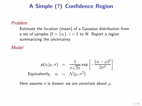
A Simple (?) Confidence Region
ProblemEstimate the location (mean) of a Gaussian distribution froma set of samples D = xi, i = 1 to N. Report a regionsummarizing the uncertainty.
Model
p(xi |µ, σ) =1
σ√2π
exp
[
−(xi − µ)2
2σ2
]
Equivalently, xi ∼ N (µ, σ2)
Here assume σ is known; we are uncertain about µ.
9 / 76

Classes of variables
• µ is the unknown we seek to estimate—the parameter. Theparameter space is the space of possible values of µ—here thereal line (perhaps bounded). Hypothesis space is a moregeneral term.
• A particular set of N data values D = xi is a sample. Thesample space is the N-dimensional space of possible samples.
Standard inferencesLet x = 1
N
∑Ni=1 xi .
• “Standard error” (rms error) is σ/√N
• “1σ” interval: x ± σ/√N with conf. level CL = 68.3%
• “2σ” interval: x ± 2σ/√N with CL = 95.4%
10 / 76

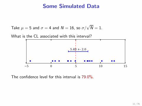
Some Simulated Data
Take µ = 5 and σ = 4 and N = 16, so σ/√N = 1.
What is the CL associated with this interval?
−5 0 5 10 15
5.49 +- 2.0
11 / 76
Some Simulated Data
Take µ = 5 and σ = 4 and N = 16, so σ/√N = 1.
What is the CL associated with this interval?
−5 0 5 10 15
5.49 +- 2.0
The confidence level for this interval is 79.0%.
11 / 76
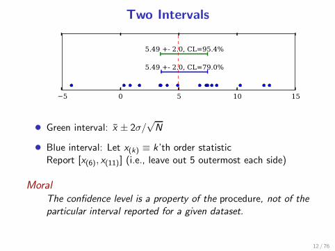
Two Intervals
−5 0 5 10 15
5.49 +- 2.0, CL=79.0%
5.49 +- 2.0, CL=95.4%
• Green interval: x ± 2σ/√N
• Blue interval: Let x(k) ≡ k ’th order statisticReport [x(6), x(11)] (i.e., leave out 5 outermost each side)
MoralThe confidence level is a property of the procedure, not of theparticular interval reported for a given dataset.
12 / 76

Performance of Intervals
Intervals for 15 datasets
−10 −5 0 5 10 15 20
13 / 76

Confidence interval for a normal meanSuppose we have a sample of N = 5 values xi ,
xi ∼ N(µ, 1)
We want to estimate µ, including some quantification ofuncertainty in the estimate: an interval with a probability attached.
Frequentist approaches: method of moments, BLUE,least-squares/χ2, maximum likelihood
Focus on likelihood (equivalent to χ2 here); this is closest to Bayes.
L(µ) = p(xi|µ)
=∏
i
1
σ√2π
e−(xi−µ)2/2σ2; σ = 1
∝ e−χ2(µ)/2
Estimate µ from maximum likelihood (minimum χ2).Define an interval and its coverage frequency from the L(µ) curve.
14 / 76
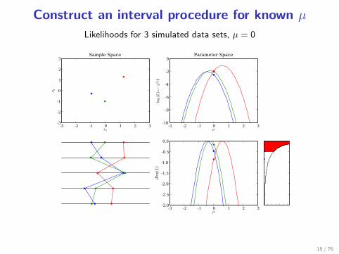
Construct an interval procedure for known µ
Likelihoods for 3 simulated data sets, µ = 0
-3 -2 -1 0 1 2 31x
-3
-2
-1
0
1
2
3
2x
Sample Space
-3 -2 -1 0 1 2 3µ
-10
-8
-6
-4
-2
0
2/2
χ−
=)L(
gol
Parameter Space
-3 -2 -1 0 1 2 3µ
-3.0
-2.5
-2.0
-1.5
-1.0
-0.5
0.0
)L(
gol
∆
15 / 76
Likelihoods for 100 simulated data sets, µ = 0
-3 -2 -1 0 1 2 31x
-3
-2
-1
0
1
2
3
2x
Sample Space
-3 -2 -1 0 1 2 3µ
-10
-8
-6
-4
-2
0
2/2
χ−
=)L(
gol
Parameter Space
-3 -2 -1 0 1 2 3µ
-3.0
-2.5
-2.0
-1.5
-1.0
-0.5
0.0
)L(
gol
∆
16 / 76

Explore dependence on µ
Likelihoods for 100 simulated data sets, µ = 3
0 1 2 3 4 5 61x
0
1
2
3
4
5
6
2x
Sample Space
0 1 2 3 4 5 6µ
-10
-8
-6
-4
-2
0
2/2
χ−
=)L(
gol
Parameter Space
0 1 2 3 4 5 6µ
-3.0
-2.5
-2.0
-1.5
-1.0
-0.5
0.0
)L(
gol
∆
Luckily the ∆ logL distribution is the same!
If it weren’t, define confidence level = maximum coverage over all µ (confidence level= conservative guarantee of coverage).
Parametric bootstrap: Skip this step; just report the coverage based on µ = µ(xi)for the observed data. Theory shows the error in the coverage falls faster than
√N.
17 / 76
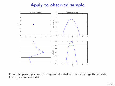
Apply to observed sample
-3 -2 -1 0 1 2 31x
-3
-2
-1
0
1
2
3
2x
Sample Space
-3 -2 -1 0 1 2 3µ
-10
-8
-6
-4
-2
0
2/2
χ−
=)L(
gol
Parameter Space
-3 -2 -1 0 1 2 3µ
-3.0
-2.5
-2.0
-1.5
-1.0
-0.5
0.0
)L(
gol
∆
Report the green region, with coverage as calculated for ensemble of hypothetical data(red region, previous slide).
18 / 76
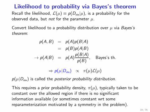
Likelihood to probability via Bayes’s theoremRecall the likelihood, L(µ) ≡ p(Dobs|µ), is a probability for theobserved data, but not for the parameter µ.
Convert likelihood to a probability distribution over µ via Bayes’stheorem:
p(A,B) = p(A)p(B |A)= p(B)p(A|B)
→ p(A|B) = p(A)p(B |A)p(B)
, Bayes’s th.
⇒ p(µ|Dobs) ∝ π(µ)L(µ)p(µ|Dobs) is called the posterior probability distribution.
This requires a prior probability density, π(µ), typically taken to beconstant over the allowed region if there is no significantinformation available (or sometimes constant wrt somereparameterization motivated by a symmetry in the problem).
19 / 76

Roles of the prior
Prior has two roles
• Incorporate any relevant prior information
• Convert likelihood from “intensity” to “measure”→ account for size of parameter space
Physical analogy
Heat Q =
∫
dr [ρ(r)c(r)]T (r)
Probability P ∝∫
dθ π(θ)L(θ)Maximum likelihood focuses on the “hottest” parameters.
Bayes focuses on the parameters with the most “heat.”
A high-T region may contain little heat if its ρc is low or if its
volume is small.
A high-L region may contain little probability if its prior is low or if
its volume is small.
20 / 76

Gaussian problem posterior distribution
For the Gaussian example, a bit of algebra (“complete the square”)gives:
L(µ) ∝∏
i
exp
[
−(xi − µ)2
2σ2
]
∝ exp
[
− (µ− x)2
2(σ/√N)2
]
The likelihood is Gaussian in µ.Flat prior → posterior density for µ is N (x , σ2/N).
21 / 76

Bayesian credible region
Normalize the likelihood for the observed sample; report the region that includes68.3% of the normalized likelihood.
-3 -2 -1 0 1 2 31x
-3
-2
-1
0
1
2
3
2x
Sample Space
-3 -2 -1 0 1 2 3µ
-10
-8
-6
-4
-2
0
2/2χ
−=)
L(gol
Parameter Space
-3 -2 -1 0 1 2 3µ
0.0
0.2
0.4
0.6
0.8
1.0
)µ(
Ldezila
mroN
22 / 76
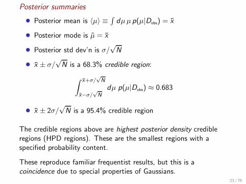
Posterior summaries
• Posterior mean is 〈µ〉 ≡∫
dµµ p(µ|Dobs) = x
• Posterior mode is µ = x
• Posterior std dev’n is σ/√N
• x ± σ/√N is a 68.3% credible region:
∫ x+σ/√N
x−σ/√N
dµ p(µ|Dobs) ≈ 0.683
• x ± 2σ/√N is a 95.4% credible region
The credible regions above are highest posterior density credibleregions (HPD regions). These are the smallest regions with aspecified probability content.
These reproduce familiar frequentist results, but this is acoincidence due to special properties of Gaussians.
23 / 76
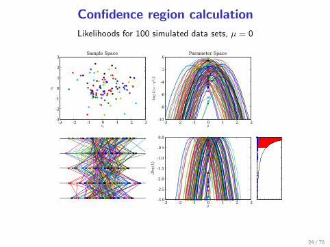
Confidence region calculation
Likelihoods for 100 simulated data sets, µ = 0
-3 -2 -1 0 1 2 31x
-3
-2
-1
0
1
2
3
2x
Sample Space
-3 -2 -1 0 1 2 3µ
-10
-8
-6
-4
-2
0
2/2
χ−
=)L(
gol
Parameter Space
-3 -2 -1 0 1 2 3µ
-3.0
-2.5
-2.0
-1.5
-1.0
-0.5
0.0
)L(
gol
∆
24 / 76

When They’ll DifferBoth approaches report µ ∈ [x − σ/
√N, x + σ/
√N], and assign
68.3% to this interval (with different meanings).
This matching is a coincidence!
When might results differ? (F = frequentist, B = Bayes)
• If F procedure doesn’t use likelihood directly• If F procedure properties depend on params (nonlinear models,
pivotal quantities)• If F properties depend on likelihood shape (conditional inference,
ancillary statistics, recognizable subsets)• If there are extra uninteresting parameters (nuisance parameters,
corrected profile likelihood, conditional inference)• If B uses important prior information
Also, for a different task—comparison of parametric models—theapproaches are qualitatively different (significance tests & infocriteria vs. Bayes factors)
25 / 76
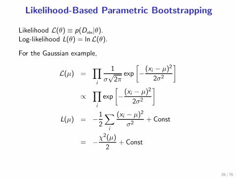
Likelihood-Based Parametric Bootstrapping
Likelihood L(θ) ≡ p(Dobs|θ).Log-likelihood L(θ) = lnL(θ).
For the Gaussian example,
L(µ) =∏
i
1
σ√2π
exp
[
−(xi − µ)2
2σ2
]
∝∏
i
exp
[
−(xi − µ)2
2σ2
]
L(µ) = −1
2
∑
i
(xi − µ)2
σ2+ Const
= −χ2(µ)
2+ Const
26 / 76
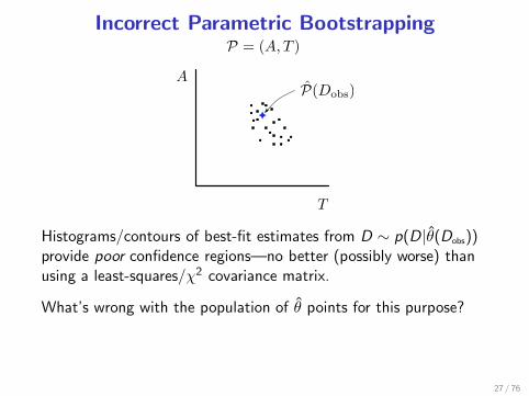
Incorrect Parametric Bootstrapping
A
T
P = (A, T )
!
P(Dobs)
Histograms/contours of best-fit estimates from D ∼ p(D|θ(Dobs))provide poor confidence regions—no better (possibly worse) thanusing a least-squares/χ2 covariance matrix.
What’s wrong with the population of θ points for this purpose?
27 / 76

Incorrect Parametric Bootstrapping
A
T
P = (A, T )
!
P(Dobs)"
Histograms/contours of best-fit estimates from D ∼ p(D|θ(Dobs))provide poor confidence regions—no better (possibly worse) thanusing a least-squares/χ2 covariance matrix.
What’s wrong with the population of θ points for this purpose?
The estimates are skewed down and to the right, indicating thetruth must be up and to the left. Do not mistake variability of theestimator with the uncertainty of the estimate!
27 / 76
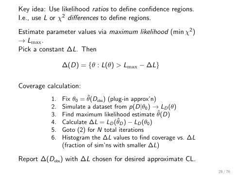
Key idea: Use likelihood ratios to define confidence regions.I.e., use L or χ2 differences to define regions.
Estimate parameter values via maximum likelihood (minχ2)→ Lmax.Pick a constant ∆L. Then
∆(D) = θ : L(θ) > Lmax −∆L
Coverage calculation:
1. Fix θ0 = θ(Dobs) (plug-in approx’n)2. Simulate a dataset from p(D|θ0) → LD(θ)3. Find maximum likelihood estimate θ(D)4. Calculate ∆L = LD(θD)− LD(θ0)5. Goto (2) for N total iterations6. Histogram the ∆L values to find coverage vs. ∆L
(fraction of sim’ns with smaller ∆L)
Report ∆(Dobs) with ∆L chosen for desired approximate CL.
28 / 76

∆L Calibration Reported Region
A
T
!
A
T
!
The CL is approximate due to:
• Monte Carlo error in calibrating ∆L
• The plug-in approximation
29 / 76

Credible Region Via Posterior SamplingMonte Carlo algorithm for finding credible regions:
1. Create a RNG that can sample θ from p(θ|Dobs)2. Draw N samples; record θi and qi = π(θi )L(µi )3. Sort the samples by the qi values4. An HPD region of probability P is the θ region spanned
by the 100P% of samples with highest qi
Note that no dataset other than Dobs is ever considered.P is a property of the particular interval reported.
A
T
!
30 / 76

Interpretations of Regions
Confidence regionFrequentist probabilities describe variability in theperformance of procedures/rules over an ensemble.
A confidence region ∆(D) with specified CL contains the trueparameter value 100CL% of the time. This quantifies theconfidence you might have that the value is in the particularinterval ∆(Dobs).
Credible regionBayesian probabilities are quantifications of the strength ofarguments—p(A|B) measures how justified one is in reasoningfrom B to A, i.e., how strongly B supports A vs. itsalternatives.
The probability within a credible region quantifies howstrongly the particular dataset we’ve observed justifiesconcluding the true parameter value is in the region.
31 / 76

Bayesian and Frequentist Inference
Brad Efron, ASA President (2005)The 250-year debate between Bayesians and frequentists isunusual among philosophical arguments in actually havingimportant practical consequences.. . . The physicists I talkedwith were really bothered by our 250 year oldBayesian-frequentist argument. Basically there’s only one wayof doing physics but there seems to be at least two ways to dostatistics, and they don’t always give the same answers.. . .
Broadly speaking, Bayesian statistics dominated 19th Centurystatistical practice while the 20th Century was morefrequentist. What’s going to happen in the 21st Century?. . . Istrongly suspect that statistics is in for a burst of new theoryand methodology, and that this burst will feature acombination of Bayesian and frequentist reasoning.. . .
32 / 76

Roderick Little, ASA President’s Address (2005)Pragmatists might argue that good statisticians can getsensible answers under Bayes or frequentist paradigms; indeedmaybe two philosophies are better than one, since they providemore tools for the statistician’s toolkit.. . . I am discomfortedby this “inferential schizophrenia.” Since the Bayesian (B)and frequentist (F) philosophies can differ even on simpleproblems, at some point decisions seem needed as to which isright. I believe our credibility as statisticians is underminedwhen we cannot agree on the fundamentals of our subject.. . .
An assessment of strengths and weaknesses of the frequentistand Bayes systems of inference suggests that calibratedBayes. . . captures the strengths of both approaches andprovides a roadmap for future advances.
33 / 76

Bayesian Fundamentals
1 Confidence intervals vs. credible intervals
2 Foundations: Logic & probability theory
3 Probability theory for data analysis: Three theorems
4 Inference with parametric modelsParameter EstimationModel Uncertainty
34 / 76

Logic—Some Essentials“Logic can be defined as the analysis and appraisal of arguments”
—Gensler, Intro to Logic
Build arguments with propositions and logicaloperators/connectives:
• Propositions: Statements that may be true or false
P : Universe can be modeled with ΛCDM
A : Ωtot ∈ [0.9, 1.1]
B : ΩΛ is not 0
B : “not B ,” i.e., ΩΛ = 0
• Connectives:
A ∧ B : A andB are both true
A ∨ B : A orB is true, or both are
35 / 76

Arguments
Argument: Assertion that an hypothesized conclusion, H, followsfrom premises, P = A,B ,C , . . . (take “,” = “and”)
Notation:
H|P : Premises P imply H
H may be deduced from PH follows from PH is true given that P is true
Arguments are (compound) propositions.
Central role of arguments → special terminology for true/false:
• A true argument is valid
• A false argument is invalid or fallacious
36 / 76

Valid vs. Sound Arguments
Content vs. form
• An argument is factually correct iff all of its premises are true(it has “good content”).
• An argument is valid iff its conclusion follows from itspremises (it has “good form”).
• An argument is sound iff it is both factually correct and valid(it has good form and content).
Deductive logic (and probability theory) addresses validity.
We want to make sound arguments. There is no formal approachfor addressing factual correctness → there is always a subjectiveelement to an argument.
37 / 76

Factual Correctness
Passing the buckAlthough logic can teach us something about validity andinvalidity, it can teach us very little about factual correctness.The question of the truth or falsity of individual statements isprimarily the subject matter of the sciences.
— Hardegree, Symbolic Logic
An open issueTo test the truth or falsehood of premisses is the task ofscience. . . . But as a matter of fact we are interested in, andmust often depend upon, the correctness of arguments whosepremisses are not known to be true.
— Copi, Introduction to Logic
38 / 76

Premises
• Facts — Things known to be true, e.g. observed data
• “Obvious” assumptions — Axioms, postulates, e.g., Euclid’sfirst 4 postulates (line segment b/t 2 points; congruency ofright angles . . . )
• “Reasonable” or “working” assumptions — E.g., Euclid’s fifthpostulate (parallel lines)
• Desperate presumption!
• Conclusions from other arguments
Premises define a fixed context in which arguments may beassessed.
Premises are considered “given”—if only for the sake of theargument!
39 / 76

Deductive and Inductive Inference
Deduction—Syllogism as prototypePremise 1: A implies HPremise 2: A is trueDeduction: ∴ H is trueH|P is valid
Induction—Analogy as prototypePremise 1: A,B ,C ,D,E all share properties x , y , zPremise 2: F has properties x , yInduction: F has property z“F has z”|P is not strictly valid, but may still be rational(likely, plausible, probable); some such arguments are strongerthan others
Boolean algebra (and/or/not over 0, 1) quantifies deduction.
Bayesian probability theory (and/or/not over [0, 1]) generalizes thisto quantify the strength of inductive arguments.
40 / 76

Deductive Logic
Assess arguments by decomposing them into parts via connectives,and assessing the parts:
Validity of A ∧ B |P
A|P A|PB |P valid invalid
B |P invalid invalid
Validity of A ∨ B |P
A|P A|PB |P valid valid
B|P valid invalid
41 / 76

Representing Deduction With 0, 1 Algebra
V (H|P) ≡ Validity of argument H|P:
V = 0 → Argument is invalid
= 1 → Argument is valid
Then deduction can be reduced to integer multiplication andaddition over 0, 1 (as in a computer):
V (A ∧ B |P) = V (A|P)V (B |P)
V (A ∨ B |P) = V (A|P) + V (B |P)− V (A ∧ B |P)
V (A|P) = 1− V (A|P)
42 / 76

Representing Induction With [0, 1] Algebra
P(H|P) ≡ strength of argument H|P
P = 0 → Argument is invalid; premises imply H
= 1 → Argument is valid
∈ (0, 1) → Degree of deducibility
Mathematical model for induction
‘AND’ (product rule): P(A ∧ B |P) = P(A|P)P(B |A ∧ P)
= P(B |P)P(A|B ∧ P)
‘OR’ (sum rule): P(A ∨ B |P) = P(A|P) + P(B |P)−P(A ∧ B |P)
‘NOT’: P(A|P) = 1− P(A|P)
43 / 76
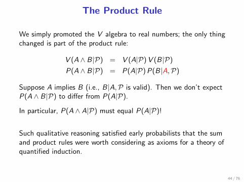
The Product Rule
We simply promoted the V algebra to real numbers; the only thingchanged is part of the product rule:
V (A ∧ B |P) = V (A|P)V (B |P)
P(A ∧ B |P) = P(A|P)P(B |A,P)
Suppose A implies B (i.e., B |A,P is valid). Then we don’t expectP(A ∧ B |P) to differ from P(A|P).
In particular, P(A ∧ A|P) must equal P(A|P)!
Such qualitative reasoning satisfied early probabilists that the sumand product rules were worth considering as axioms for a theory ofquantified induction.
44 / 76
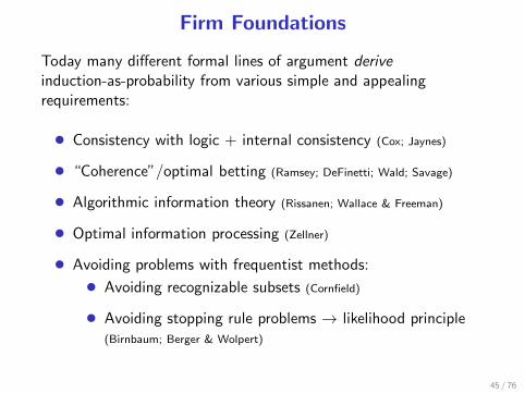
Firm Foundations
Today many different formal lines of argument deriveinduction-as-probability from various simple and appealingrequirements:
• Consistency with logic + internal consistency (Cox; Jaynes)
• “Coherence”/optimal betting (Ramsey; DeFinetti; Wald; Savage)
• Algorithmic information theory (Rissanen; Wallace & Freeman)
• Optimal information processing (Zellner)
• Avoiding problems with frequentist methods:
• Avoiding recognizable subsets (Cornfield)
• Avoiding stopping rule problems → likelihood principle(Birnbaum; Berger & Wolpert)
45 / 76

Interpreting Bayesian Probabilities
If we like there is no harm in saying that a probability expresses adegree of reasonable belief. . . . ‘Degree of confirmation’ has beenused by Carnap, and possibly avoids some confusion. But whateververbal expression we use to try to convey the primitive idea, thisexpression cannot amount to a definition. Essentially the notioncan only be described by reference to instances where it is used. Itis intended to express a kind of relation between data andconsequence that habitually arises in science and in everyday life,and the reader should be able to recognize the relation fromexamples of the circumstances when it arises.
— Sir Harold Jeffreys, Scientific Inference
46 / 76
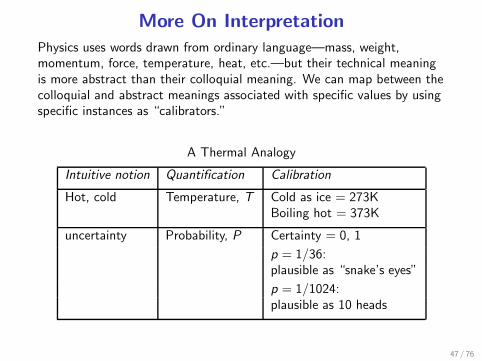
More On Interpretation
Physics uses words drawn from ordinary language—mass, weight,momentum, force, temperature, heat, etc.—but their technical meaningis more abstract than their colloquial meaning. We can map between thecolloquial and abstract meanings associated with specific values by usingspecific instances as “calibrators.”
A Thermal Analogy
Intuitive notion Quantification Calibration
Hot, cold Temperature, T Cold as ice = 273KBoiling hot = 373K
uncertainty Probability, P Certainty = 0, 1
p = 1/36:plausible as “snake’s eyes”
p = 1/1024:plausible as 10 heads
47 / 76

A Bit More On Interpretation
Bayesian
Probability quantifies uncertainty in an inductive inference. p(x)
describes how probability is distributed over the possible values x
might have taken in the single case before us:
P
x
p is distributed
x has a single,uncertain value
Frequentist
Probabilities are always (limiting) rates/proportions/frequencies
that quantify variability in a sequence of trials. p(x) describes how
the values of x would be distributed among infinitely many trials:
x is distributed
x
P
48 / 76
Bayesian Fundamentals
1 Confidence intervals vs. credible intervals
2 Foundations: Logic & probability theory
3 Probability theory for data analysis: Three theorems
4 Inference with parametric modelsParameter EstimationModel Uncertainty
49 / 76

Arguments Relating
Hypotheses, Data, and Models
We seek to appraise scientific hypotheses in light of observed dataand modeling assumptions.
Consider the data and modeling assumptions to be the premises ofan argument with each of various hypotheses, Hi , as conclusions:Hi |Dobs, I . (I = “background information,” everything deemedrelevant besides the observed data)
P(Hi |Dobs, I ) measures the degree to which (Dobs, I ) allow one todeduce Hi . It provides an ordering among arguments for various Hi
that share common premises.
Probability theory tells us how to analyze and appraise theargument, i.e., how to calculate P(Hi |Dobs, I ) from simpler,hopefully more accessible probabilities.
50 / 76
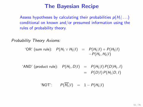
The Bayesian Recipe
Assess hypotheses by calculating their probabilities p(Hi | . . .)conditional on known and/or presumed information using therules of probability theory.
Probability Theory Axioms:
‘OR’ (sum rule): P(H1 ∨ H2|I ) = P(H1|I ) + P(H2|I )−P(H1,H2|I )
‘AND’ (product rule): P(H1,D|I ) = P(H1|I )P(D|H1, I )
= P(D|I )P(H1|D, I )
‘NOT’: P(H1|I ) = 1− P(H1|I )
51 / 76

Three Important Theorems
Bayes’s Theorem (BT)Consider P(Hi ,Dobs|I ) using the product rule:
P(Hi ,Dobs|I ) = P(Hi |I )P(Dobs|Hi , I )
= P(Dobs|I )P(Hi |Dobs, I )
Solve for the posterior probability:
P(Hi |Dobs, I ) = P(Hi |I )P(Dobs|Hi , I )
P(Dobs|I )
Theorem holds for any propositions, but for hypotheses &data the factors have names:
posterior ∝ prior × likelihood
norm. const. P(Dobs|I ) = prior predictive
52 / 76
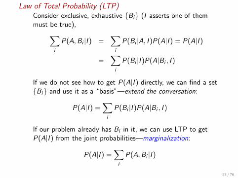
Law of Total Probability (LTP)Consider exclusive, exhaustive Bi (I asserts one of themmust be true),
∑
i
P(A,Bi |I ) =∑
i
P(Bi |A, I )P(A|I ) = P(A|I )
=∑
i
P(Bi |I )P(A|Bi , I )
If we do not see how to get P(A|I ) directly, we can find a setBi and use it as a “basis”—extend the conversation:
P(A|I ) =∑
i
P(Bi |I )P(A|Bi , I )
If our problem already has Bi in it, we can use LTP to getP(A|I ) from the joint probabilities—marginalization:
P(A|I ) =∑
i
P(A,Bi |I )
53 / 76
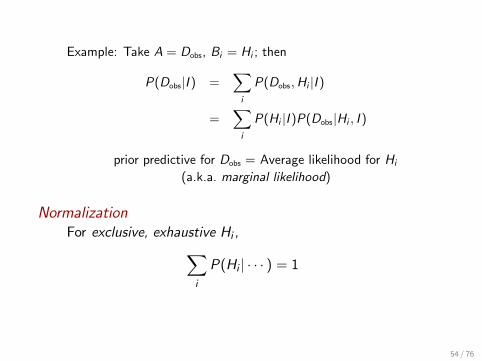
Example: Take A = Dobs, Bi = Hi ; then
P(Dobs|I ) =∑
i
P(Dobs,Hi |I )
=∑
i
P(Hi |I )P(Dobs|Hi , I )
prior predictive for Dobs = Average likelihood for Hi
(a.k.a. marginal likelihood)
NormalizationFor exclusive, exhaustive Hi ,
∑
i
P(Hi | · · · ) = 1
54 / 76
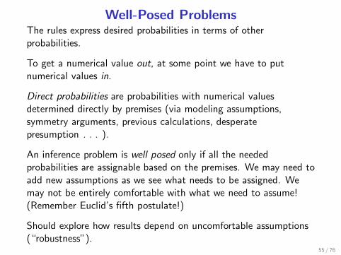
Well-Posed ProblemsThe rules express desired probabilities in terms of otherprobabilities.
To get a numerical value out, at some point we have to putnumerical values in.
Direct probabilities are probabilities with numerical valuesdetermined directly by premises (via modeling assumptions,symmetry arguments, previous calculations, desperatepresumption . . . ).
An inference problem is well posed only if all the neededprobabilities are assignable based on the premises. We may need toadd new assumptions as we see what needs to be assigned. Wemay not be entirely comfortable with what we need to assume!(Remember Euclid’s fifth postulate!)
Should explore how results depend on uncomfortable assumptions(“robustness”).
55 / 76
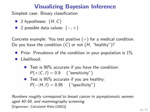
Visualizing Bayesian InferenceSimplest case: Binary classification
• 2 hypotheses: H,C• 2 possible data values: −,+
Concrete example: You test positive (+) for a medical condition.Do you have the condition (C ) or not (H, “healthy”)?
• Prior: Prevalence of the condition in your population is 1%
• Likelihood:
• Test is 90% accurate if you have the condition:P(+|C , I ) = 0.9 (“sensitivity”)
• Test is 95% accurate if you are healthy:P(−|H, I ) = 0.95 (“specificity”)
Numbers roughly correspond to breast cancer in asymptomatic womenaged 40–50, and mammography screening[Gigerenzer, Calculated Risks (2002)]
56 / 76

Probability “Tree”
H or CP=1
HP=0.99
CP=0.01
H–P=0.9405
H+P=0.0495
C–P=0.001
C+P=0.009
–P=0.9415
+P=0.0585
x0.99 x0.01
x0.95 x0.05 x0.1 x0.9
A or BP=1
Proposition
probability=
x0.01 =AND
(product)
=OR
(sum)P (Hi|I)
P (Hi, D|I) =
P (Hi|I)P (D|Hi, I)
P (D|I) =∑
i
P (Hi, D|I)
P (C|+, I) =0.009
0.0585≈ 0.15
P (H1 ∨H2|I)
∗Not really a tree; really a graph or part of a lattice
57 / 76
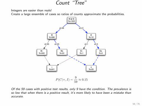
Count “Tree”Integers are easier than reals!Create a large ensemble of cases so ratios of counts approximate the probabilities.
H or CN=1000
HN=990
CN=10
H–N=940
H+N=50
C–N=1
C+N=9
–N=941
+N=59
x0.99 x0.01
x0.95 x0.05 x0.1 x0.9
P (C|+, I) =9
59≈ 0.15
Of the 59 cases with positive test results, only 9 have the condition. The prevalence is
so low that when there is a positive result, it’s more likely to have been a mistake than
accurate.
58 / 76
Bayesian Fundamentals
1 Confidence intervals vs. credible intervals
2 Foundations: Logic & probability theory
3 Probability theory for data analysis: Three theorems
4 Inference with parametric modelsParameter EstimationModel Uncertainty
59 / 76

Inference With Parametric Models
Models Mi (i = 1 to N), each with parameters θi , each imply asampling dist’n (conditional predictive dist’n for possible data):
p(D|θi ,Mi )
The θi dependence when we fix attention on the observed data isthe likelihood function:
Li(θi) ≡ p(Dobs|θi ,Mi )
We may be uncertain about i (model uncertainty) or θi (parameteruncertainty).
Henceforth we will only consider the actually observed data, so we dropthe cumbersome subscript: D = Dobs.
60 / 76

Three Classes of Problems
Parameter EstimationPremise = choice of model (pick specific i)→ What can we say about θi?
Model Assessment
• Model comparison: Premise = Mi→ What can we say about i?
• Model adequacy/GoF: Premise = M1∨ “all” alternatives→ Is M1 adequate?
Model AveragingModels share some common params: θi = φ, ηi→ What can we say about φ w/o committing to one model?(Examples: systematic error, prediction)
61 / 76

Parameter Estimation
Problem statementI = Model M with parameters θ (+ any add’l info)
Hi = statements about θ; e.g. “θ ∈ [2.5, 3.5],” or “θ > 0”
Probability for any such statement can be found using aprobability density function (PDF) for θ:
P(θ ∈ [θ, θ + dθ]| · · · ) = f (θ)dθ
= p(θ| · · · )dθ
Posterior probability density
p(θ|D,M) =p(θ|M) L(θ)
∫
dθ p(θ|M) L(θ)
62 / 76
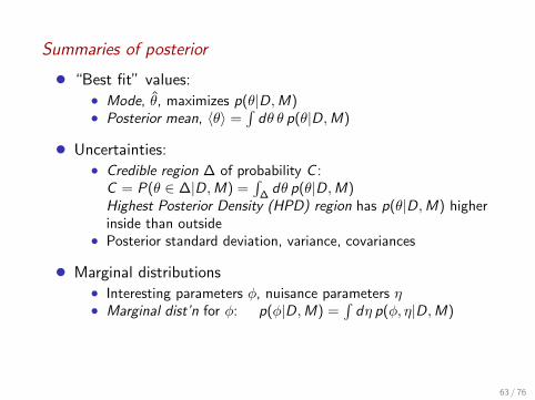
Summaries of posterior
• “Best fit” values:• Mode, θ, maximizes p(θ|D,M)• Posterior mean, 〈θ〉 =
∫
dθ θ p(θ|D,M)
• Uncertainties:• Credible region ∆ of probability C :
C = P(θ ∈ ∆|D,M) =∫
∆dθ p(θ|D,M)
Highest Posterior Density (HPD) region has p(θ|D,M) higherinside than outside
• Posterior standard deviation, variance, covariances
• Marginal distributions• Interesting parameters φ, nuisance parameters η• Marginal dist’n for φ: p(φ|D,M) =
∫
dη p(φ, η|D,M)
63 / 76

Nuisance Parameters and Marginalization
To model most data, we need to introduce parameters besidesthose of ultimate interest: nuisance parameters.
ExampleWe have data from measuring a rate r = s + b that is a sumof an interesting signal s and a background b.
We have additional data just about b.
What do the data tell us about s?
64 / 76

Marginal posterior distribution
To summarize implications for s, accounting for b uncertainty,marginalize:
p(s|D,M) =
∫
db p(s, b|D,M)
∝ p(s|M)
∫
db p(b|s)L(s, b)
= p(s|M)Lm(s)
with Lm(s) the marginal likelihood for s:
Lm(s) ≡∫
db p(b|s)L(s, b)
65 / 76

Marginalization vs. Profiling
For insight: Suppose the prior is broad compared to the likelihood→ for a fixed s, we can accurately estimate b with max likelihoodbs , with small uncertainty δbs .
Lm(s) ≡∫
db p(b|s)L(s, b)
≈ p(bs |s) L(s, bs) δbsbest b given s
b uncertainty given s
Profile likelihood Lp(s) ≡ L(s, bs) gets weighted by a parameterspace volume factor
E.g., Gaussians: s = r − b, σ2s = σ2
r + σ2b
Background subtraction is a special case of background marginalization.
66 / 76

Bivariate normals: Lm ∝ Lp
s
bbs
1.2
0
0.2
0.4
0.6
0.8
1
b
L(s
,b)/L
(s,b
s)
δbs is const. vs. s
⇒ Lm ∝ Lp
67 / 76

Flared/skewed/bannana-shaped: Lm and Lp differ
Lp(s) Lm(s)
s
b
bs
s
b
bs
Lp(s) Lm(s)
General result: For a linear (in params) model sampled withGaussian noise, and flat priors, Lm ∝ Lp.Otherwise, they will likely differ.
In measurement error problems (future lecture!) the difference canbe dramatic.
68 / 76

Many Roles for MarginalizationEliminate nuisance parameters
p(φ|D,M) =
∫
dη p(φ, η|D,M)
Propagate uncertainty
Model has parameters θ; what can we infer about F = f (θ)?
p(F |D,M) =
∫
dθ p(F , θ|D,M) =
∫
dθ p(θ|D,M) p(F |θ,M)
=
∫
dθ p(θ|D,M) δ[F − f (θ)] [single-valued case]
Prediction
Given a model with parameters θ and present data D, predict future
data D ′ (e.g., for experimental design):
p(D ′|D,M) =
∫
dθ p(D ′, θ|D,M) =
∫
dθ p(θ|D,M) p(D ′|θ,M)
Model comparison. . .69 / 76

Model ComparisonProblem statement
I = (M1 ∨M2 ∨ . . .) — Specify a set of models.Hi = Mi — Hypothesis chooses a model.
Posterior probability for a model
p(Mi |D, I ) = p(Mi |I )p(D|Mi , I )
p(D|I )∝ p(Mi |I )L(Mi )
But L(Mi) = p(D|Mi) =∫
dθi p(θi |Mi)p(D|θi ,Mi ).
Likelihood for model = Average likelihood for its parameters
L(Mi) = 〈L(θi )〉
Varied terminology: Prior predictive = Average likelihood = Globallikelihood = Marginal likelihood = (Weight of) Evidence for model
70 / 76

Odds and Bayes factors
A ratio of probabilities for two propositions using the samepremises is called the odds favoring one over the other:
Oij ≡ p(Mi |D, I )
p(Mj |D, I )
=p(Mi |I )p(Mj |I )
× p(D|Mi , I )
p(D|Mj , I )
The data-dependent part is called the Bayes factor:
Bij ≡p(D|Mi , I )
p(D|Mj , I )
It is a likelihood ratio; the BF terminology is usually reserved forcases when the likelihoods are marginal/average likelihoods.
71 / 76
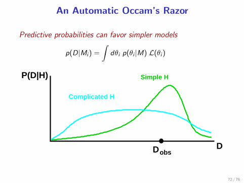
An Automatic Occam’s Razor
Predictive probabilities can favor simpler models
p(D|Mi) =
∫
dθi p(θi |M) L(θi)
DobsD
P(D|H)
Complicated H
Simple H
72 / 76

The Occam Factorp, L
θ∆θ
δθPrior
Likelihood
p(D|Mi) =
∫
dθi p(θi |M) L(θi) ≈ p(θi |M)L(θi )δθi
≈ L(θi)δθi∆θi
= Maximum Likelihood× Occam Factor
Models with more parameters often make the data moreprobable — for the best fit
Occam factor penalizes models for “wasted” volume ofparameter space
Quantifies intuition that models shouldn’t require fine-tuning
73 / 76

Model Averaging
Problem statementI = (M1 ∨M2 ∨ . . .) — Specify a set of modelsModels all share a set of “interesting” parameters, φEach has different set of nuisance parameters ηi (or differentprior info about them)Hi = statements about φ
Model averagingCalculate posterior PDF for φ:
p(φ|D, I ) =∑
i
p(Mi |D, I ) p(φ|D,Mi )
∝∑
i
L(Mi )
∫
dηi p(φ, ηi |D,Mi)
The model choice is a (discrete) nuisance parameter here.
74 / 76

Theme: Parameter Space Volume
Bayesian calculations sum/integrate over parameter/hypothesisspace!
(Frequentist calculations average over sample space & typically optimize
over parameter space.)
• Credible regions integrate over parameter space.
• Marginalization weights the profile likelihood by a volumefactor for the nuisance parameters.
• Model likelihoods have Occam factors resulting fromparameter space volume factors.
Many virtues of Bayesian methods can be attributed to thisaccounting for the “size” of parameter space. This idea does notarise naturally in frequentist statistics (but it can be added “byhand”).
75 / 76
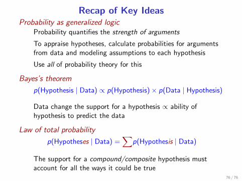
Recap of Key IdeasProbability as generalized logic
Probability quantifies the strength of arguments
To appraise hypotheses, calculate probabilities for argumentsfrom data and modeling assumptions to each hypothesis
Use all of probability theory for this
Bayes’s theorem
p(Hypothesis | Data) ∝ p(Hypothesis)× p(Data | Hypothesis)
Data change the support for a hypothesis ∝ ability ofhypothesis to predict the data
Law of total probability
p(Hypotheses | Data) =∑
p(Hypothesis | Data)
The support for a compound/composite hypothesis mustaccount for all the ways it could be true
76 / 76