introduction to coding theoryconrado/docencia/codigos.pdf · 2009-06-11 · introduction to channel...
TRANSCRIPT
1. Introduction to Channel Coding
Gadiel Seroussi/Coding Theory/September 8, 2008 1
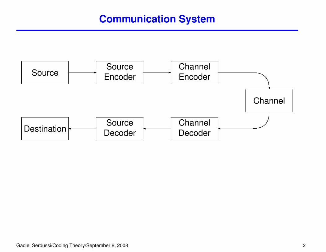
Communication System
Source -SourceEncoder
-ChannelEncoder
?
Channel
�ChannelDecoder
�Source
Decoder�Destination
Gadiel Seroussi/Coding Theory/September 8, 2008 2

Communication System
Source -SourceEncoder
-ChannelEncoder
?
Channel
�ChannelDecoder
�Source
Decoder�Destination
source coding channel coding
Gadiel Seroussi/Coding Theory/September 8, 2008 3
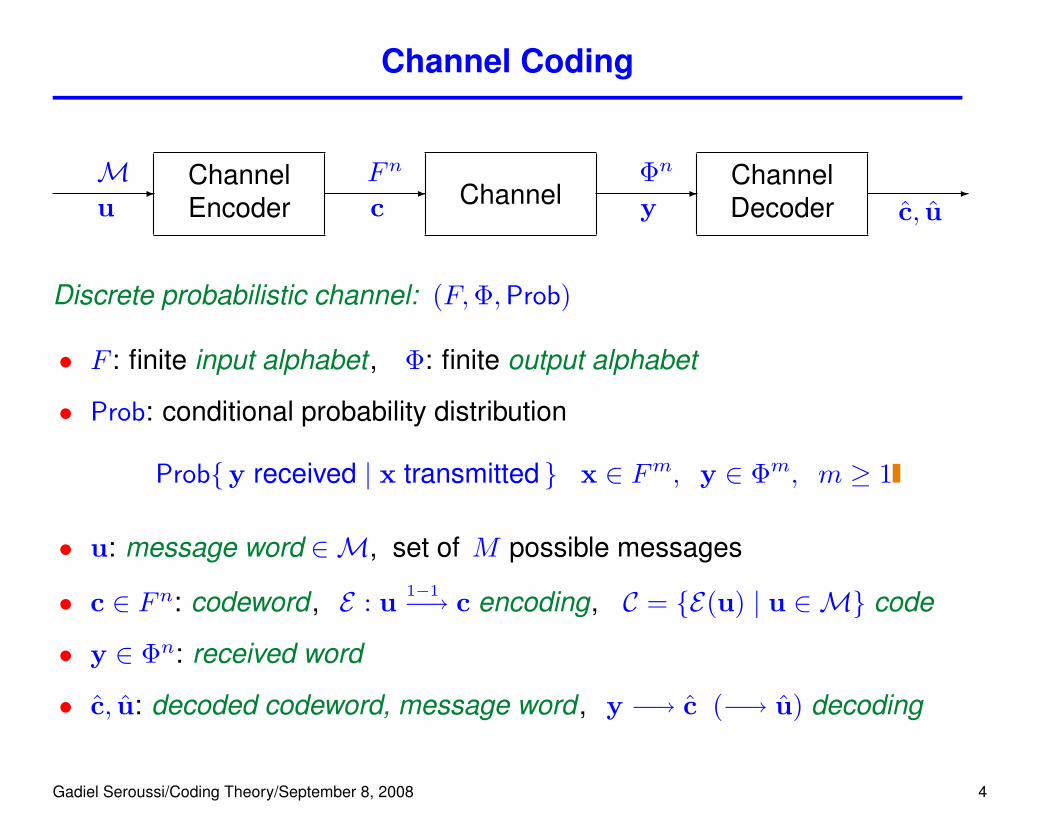
Channel Coding
-
uChannelEncoder
-
c Channel -
yChannelDecoder
-
c, u
Discrete probabilistic channel: (F,Φ,Prob)
• F : finite input alphabet , Φ: finite output alphabet
• Prob: conditional probability distribution
Prob{y received | x transmitted } x ∈ Fm, y ∈ Φm, m ≥ 1
M Fn Φn
• u: message word ∈M, set of M possible messages
• c ∈ Fn: codeword , E : u 1−1−→ c encoding, C = {E(u) | u ∈M} code
• y ∈ Φn: received word
• c, u: decoded codeword, message word , y −→ c (−→ u) decoding
Gadiel Seroussi/Coding Theory/September 8, 2008 4
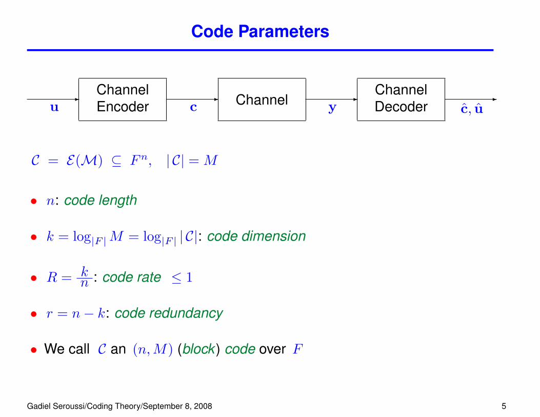
Code Parameters
-
uChannelEncoder
-
c Channel -
yChannelDecoder
-
c, u
C = E(M) ⊆ Fn, | C| = M
• n: code length
• k = log|F |M = log|F | | C|: code dimension
• R = kn : code rate ≤ 1
• r = n− k: code redundancy
• We call C an (n,M) (block ) code over F
Gadiel Seroussi/Coding Theory/September 8, 2008 5
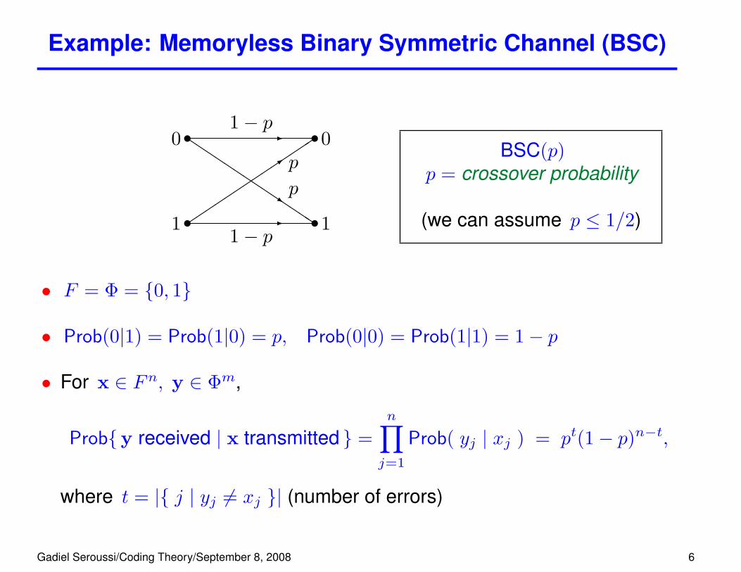
Example: Memoryless Binary Symmetric Channel (BSC)
1 v
0 v
v1
v0
-
1− p
-1− p
��������������
3
p
QQQQQQQQQQQQQQ
s
pBSC(p)
p = crossover probability
(we can assume p ≤ 1/2)
• F = Φ = {0, 1}
• Prob(0|1) = Prob(1|0) = p, Prob(0|0) = Prob(1|1) = 1− p
• For x ∈ Fn, y ∈ Φm,
Prob{y received | x transmitted } =n∏j=1
Prob( yj | xj ) = pt(1− p)n−t,
where t = |{ j | yj 6= xj }| (number of errors)
Gadiel Seroussi/Coding Theory/September 8, 2008 6
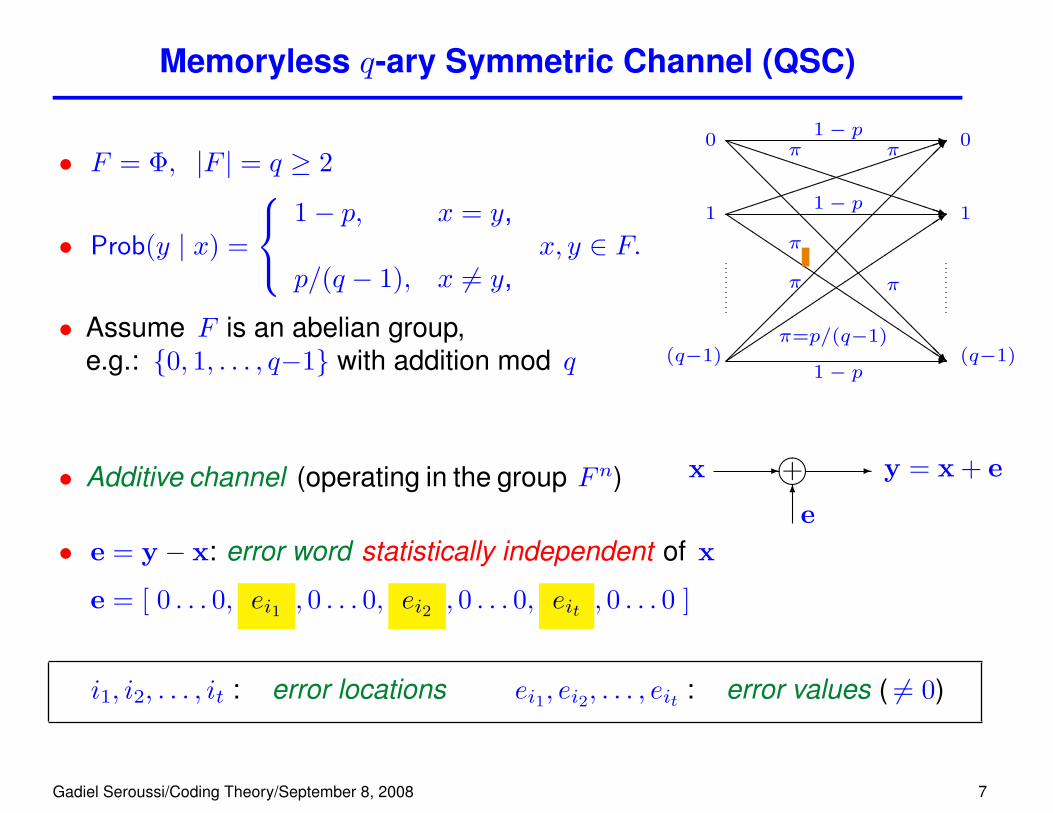
Memoryless q-ary Symmetric Channel (QSC)
• F = Φ, |F | = q ≥ 2
• Prob(y | x) =
1− p, x = y,
p/(q − 1), x 6= y,x, y ∈ F.
• Assume F is an abelian group,e.g.: {0, 1, . . . , q−1} with addition mod q -�
����������������3
������������������
QQQQQQQQQQQQQQQQQs
-����������
�������1PPPPPPPPPPPPPPPPPq
-@@@@@@@@@@@@@@@@@R(q−1)
1
0
(q−1)
1
01− p
1− p
1− p
π π
π
π π
π=p/(q−1)
• Additive channel (operating in the group Fn) ����+x - - y = x + e6
e• e = y − x: error word statistically independent of x
e = [ 0 . . . 0, ei1 , 0 . . . 0, ei2 , 0 . . . 0, eit , 0 . . . 0 ]
i1, i2, . . . , it : error locations ei1, ei2, . . . , eit : error values ( 6= 0)
Gadiel Seroussi/Coding Theory/September 8, 2008 7
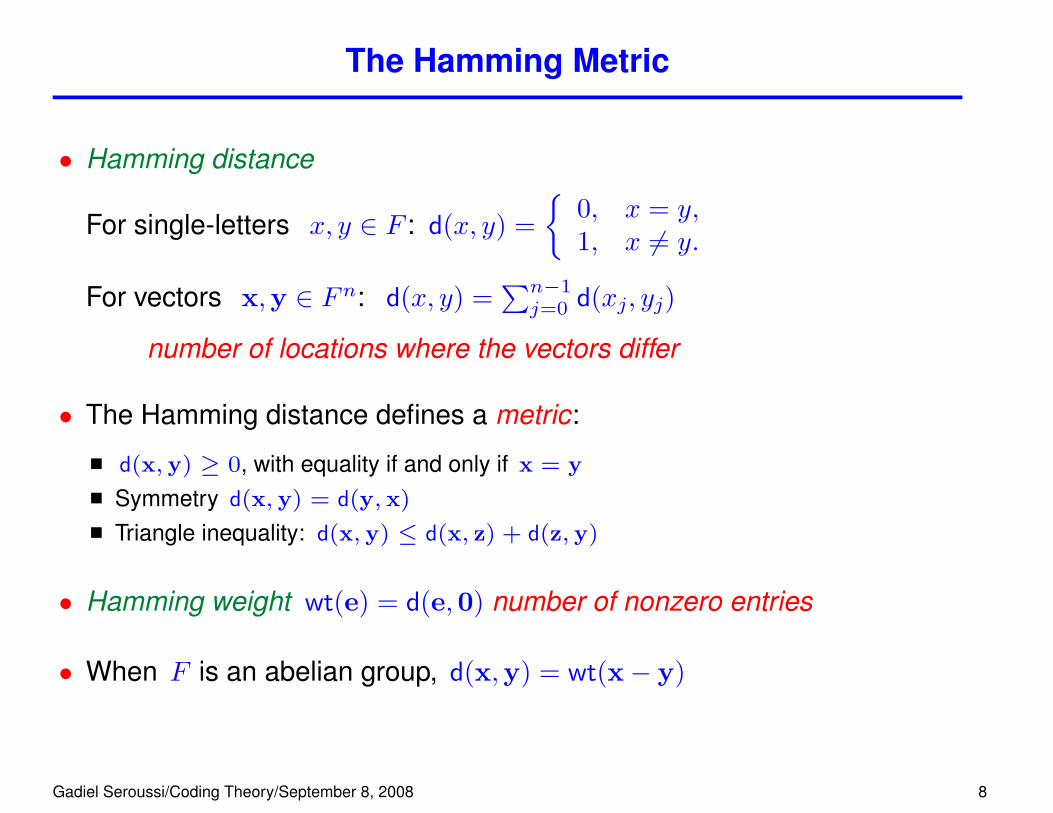
The Hamming Metric
• Hamming distance
For single-letters x, y ∈ F : d(x, y) ={
0, x = y,1, x 6= y.
For vectors x,y ∈ Fn: d(x, y) =∑n−1j=0 d(xj, yj)
number of locations where the vectors differ
• The Hamming distance defines a metric:
d(x, y) ≥ 0, with equality if and only if x = y
Symmetry d(x, y) = d(y, x)
Triangle inequality: d(x, y) ≤ d(x, z) + d(z, y)
• Hamming weight wt(e) = d(e,0) number of nonzero entries
• When F is an abelian group, d(x,y) = wt(x− y)
Gadiel Seroussi/Coding Theory/September 8, 2008 8
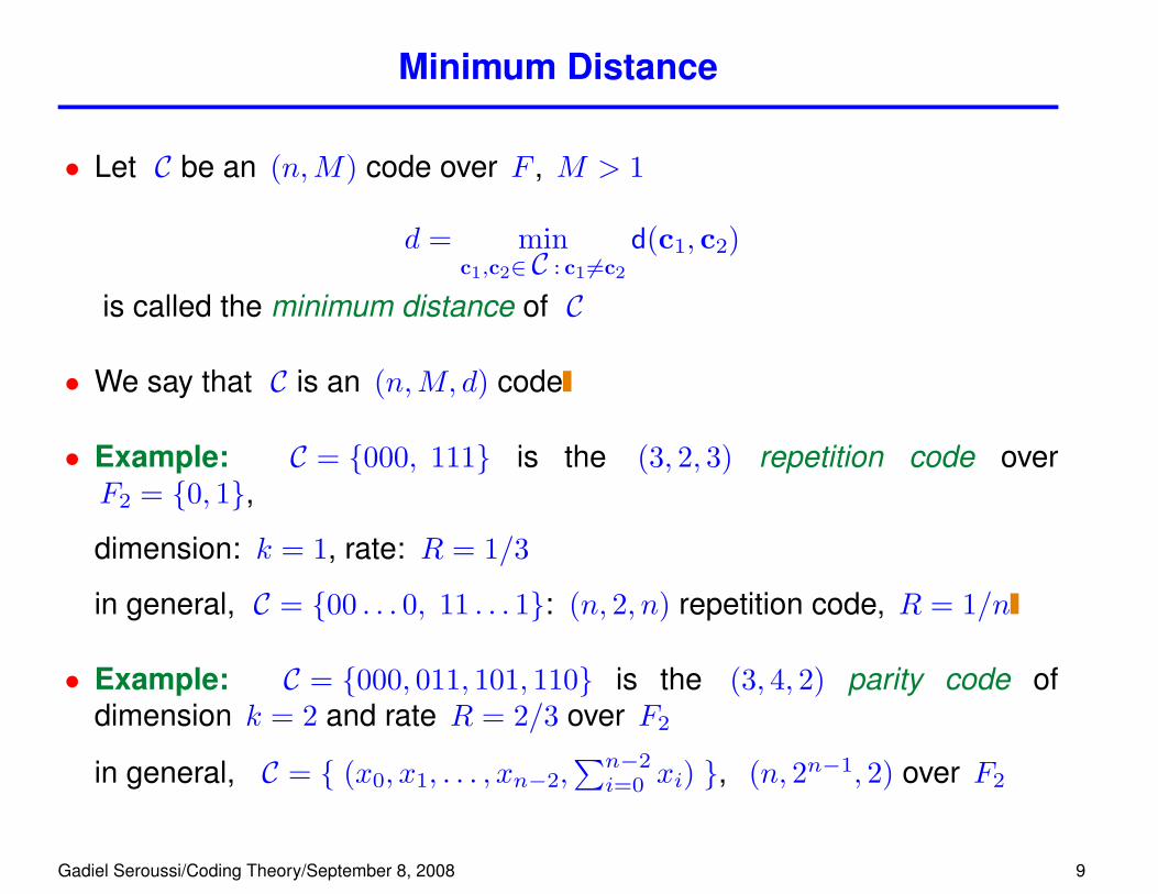
Minimum Distance
• Let C be an (n,M) code over F , M > 1
d = minc1,c2∈ C : c1 6=c2
d(c1, c2)
is called the minimum distance of C
• We say that C is an (n,M, d) code
• Example: C = {000, 111} is the (3, 2, 3) repetition code overF2 = {0, 1},
dimension: k = 1, rate: R = 1/3
in general, C = {00 . . . 0, 11 . . . 1}: (n, 2, n) repetition code, R = 1/n
• Example: C = {000, 011, 101, 110} is the (3, 4, 2) parity code ofdimension k = 2 and rate R = 2/3 over F2
in general, C = { (x0, x1, . . . , xn−2,∑n−2i=0 xi) }, (n, 2n−1, 2) over F2
Gadiel Seroussi/Coding Theory/September 8, 2008 9

Decoding
• C : (n,M, d) over F , used on channel S = (F,Φ,Prob)
• A decoder for C on S is a function
D : Φn −→ C.
• Decoding error probability of D is
Perr = maxc∈ C
Perr(c) ,
where
Perr(c) =∑
y : D(y) 6=c
Prob{y received | c transmitted } .
goal: find encoders (codes) and decoders that make Perr small
Gadiel Seroussi/Coding Theory/September 8, 2008 10

Decoding example
• Example: C = (3, 2, 3) binary repetition code, channel S = BSC(p)
Decoder D defined by
D(000) = D(001) = D(010) = D(100) = 000
D(011) = D(101) = D(110) = D(111) = 111Error probability
Perr = Perr(000) = Perr(111) =(
32
)p2(1− p) +
(33
)p3
= 3p2 − 3p3 + p3 = p− p(1− p)(1− 2p) .
• Perr < p for p < 1/2 ⇒ coding improved message error probability
but information rate is 1/3!
In general, for the repetition code, we have Perr → 0 exponentially (prove!), butR = 1/n→ 0 as n→∞ — can we do better?
goal: find encoders (codes) and decoders that make Perr smallwith minimal decrease in information rate
Gadiel Seroussi/Coding Theory/September 8, 2008 11
Maximum Likelihood and Maximum a Posteriori Decoding
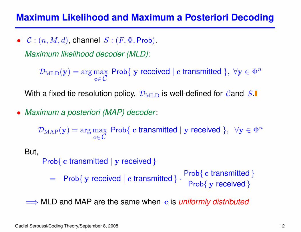
• C : (n,M, d), channel S : (F,Φ,Prob).
Maximum likelihood decoder (MLD):
DMLD(y) = arg maxc∈ C
Prob{ y received | c transmitted }, ∀y ∈ Φn
With a fixed tie resolution policy, DMLD is well-defined for Cand S.
• Maximum a posteriori (MAP) decoder :
DMAP(y) = arg maxc∈ C
Prob{ c transmitted | y received }, ∀y ∈ Φn
But,Prob{ c transmitted | y received }
= Prob{y received | c transmitted } · Prob{ c transmitted }Prob{y received }
=⇒ MLD and MAP are the same when c is uniformly distributed
Gadiel Seroussi/Coding Theory/September 8, 2008 12
MLD on the BSC
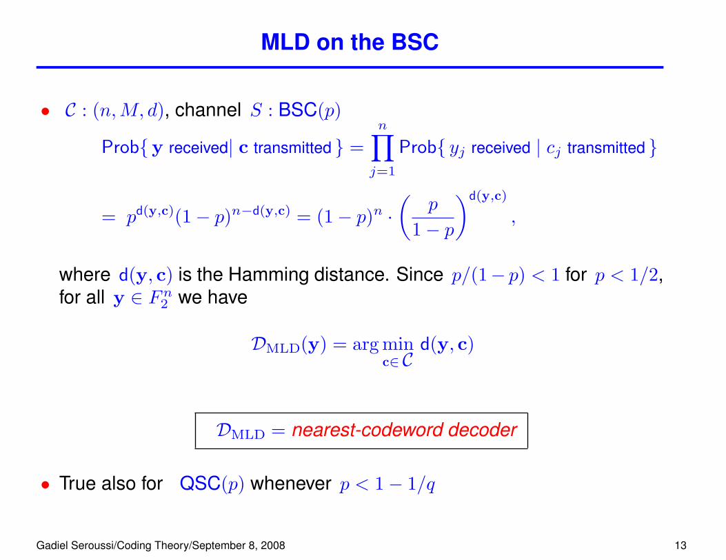
• C : (n,M, d), channel S : BSC(p)
Prob{y received| c transmitted } =n∏j=1
Prob{ yj received | cj transmitted }
= pd(y,c)(1− p)n−d(y,c) = (1− p)n ·(
p
1− p
)d(y,c)
,
where d(y, c) is the Hamming distance. Since p/(1− p) < 1 for p < 1/2,for all y ∈ Fn2 we have
DMLD(y) = arg minc∈ C
d(y, c)
DMLD = nearest-codeword decoder
• True also for QSC(p) whenever p < 1− 1/q
Gadiel Seroussi/Coding Theory/September 8, 2008 13
Capacity of the BSC
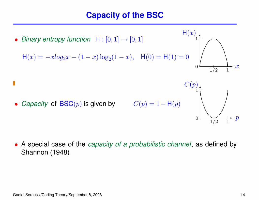
• Binary entropy function H : [0, 1]→ [0, 1]
H(x) = −xlog2x− (1− x) log2(1− x), H(0) = H(1) = 0-
6H(x)
0
1
1/2 1x
• Capacity of BSC(p) is given by C(p) = 1−H(p)
-
6C(p)
0
1
1/2 1p
• A special case of the capacity of a probabilistic channel , as defined byShannon (1948)
Gadiel Seroussi/Coding Theory/September 8, 2008 14

Shannon Coding Theorems for the BSC
Theorem. (Shannon Coding Theorem for the BSC – 1948.) Let S =BSC(p) and let R be a real number in the range 0 ≤ R < C(p). Thereexists an infinite sequence of (ni,Mi) block codes over F2, i = 1, 2, · · ·,such that (log2Mi)/ni ≥ R and, for MLD for those codes (with respect toS), the probability Perr → 0 as i→∞.
Proof. By a random coding argument. Non-constructive!
Theorem. (Shannon Converse Coding Theorem for the BSC – 1948.) LetS = BSC(p) and let R > C(p). Consider any infinite sequence { Ci :(ni,Mi)} of block codes over F2, i = 1, 2, · · ·, such that (log2Mi)/ni ≥ Rand n1 < n2 < · · · < ni < · · ·. Then, for any decoding scheme for { Ci}(with respect to S), the probability Perr → 1 as i→∞.
Proof. (Loose argument.)
Gadiel Seroussi/Coding Theory/September 8, 2008 15
Error Correction
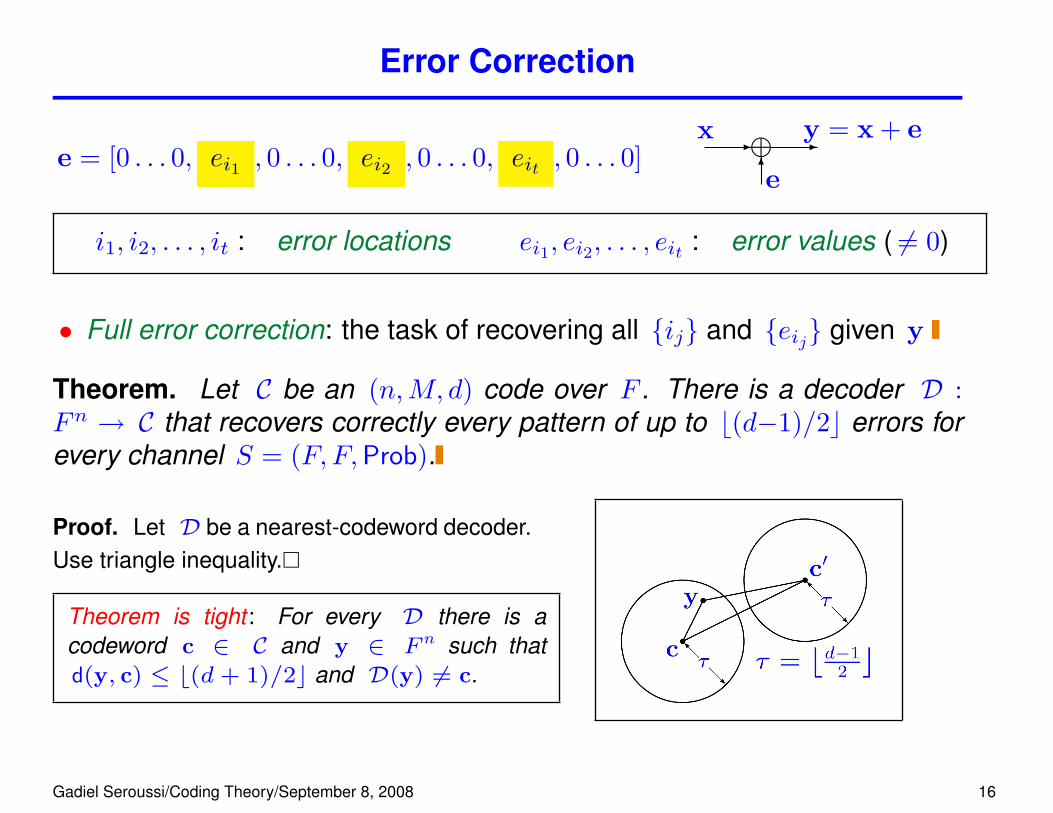
e = [0 . . . 0, ei1 , 0 . . . 0, ei2 , 0 . . . 0, eit , 0 . . . 0]m+x
- -y = x + e
6
e
i1, i2, . . . , it : error locations ei1, ei2, . . . , eit : error values ( 6= 0)
• Full error correction: the task of recovering all {ij} and {eij} given y
Theorem. Let C be an (n,M, d) code over F . There is a decoder D :Fn → C that recovers correctly every pattern of up to b(d−1)/2c errors forevery channel S = (F, F,Prob).
Proof. Let D be a nearest-codeword decoder.Use triangle inequality.�
Theorem is tight : For every D there is acodeword c ∈ C and y ∈ F n such thatd(y, c) ≤ b(d+ 1)/2c and D(y) 6= c.
Gadiel Seroussi/Coding Theory/September 8, 2008 16
Error Correction Examples
• Binary (n, 2, n) repetition code. Nearest-codeword decoding corrects upto b(n− 1)/2c errors (take majority vote).
• Binary (n, 2n−1, 2) parity code cannot correct single errors: (11100 . . . 0)is at distance 1 from codewords (11000 . . . 0) and (10100 . . . 0)
Gadiel Seroussi/Coding Theory/September 8, 2008 17

Error Detection
• Generalize the definition of a decoder to D : Fn → C ∪ {’E’}, where ’E’means “I found errors, but don’t know what they are”
Theorem. Let C be an (n,M, d) code over F . There is a decoderD : Fn → C ∪ {’E’} that detects (correctly) every pattern of up to d−1
errors.
Proof. D(y) =
y if y ∈ C
’E’ otherwise.
Example: Binary (n, 2n−1, 2) parity code can detect single errors (asingle bit error maps an even parity word to an odd parity one)
Gadiel Seroussi/Coding Theory/September 8, 2008 18
Combined correction/detection
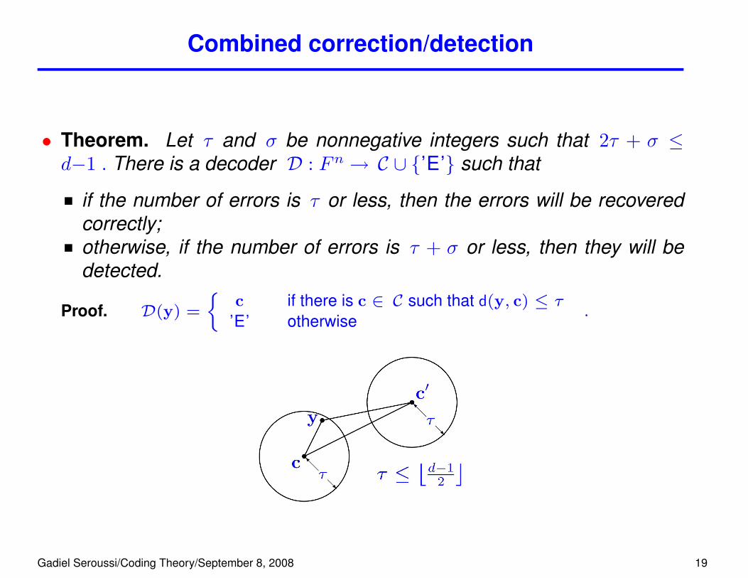
• Theorem. Let τ and σ be nonnegative integers such that 2τ + σ ≤d−1 . There is a decoder D : Fn → C ∪ {’E’} such that
if the number of errors is τ or less, then the errors will be recoveredcorrectly;otherwise, if the number of errors is τ + σ or less, then they will bedetected.
Proof. D(y) =
c if there is c ∈ C such that d(y, c) ≤ τ
’E’ otherwise.
Gadiel Seroussi/Coding Theory/September 8, 2008 19
Erasure Correction
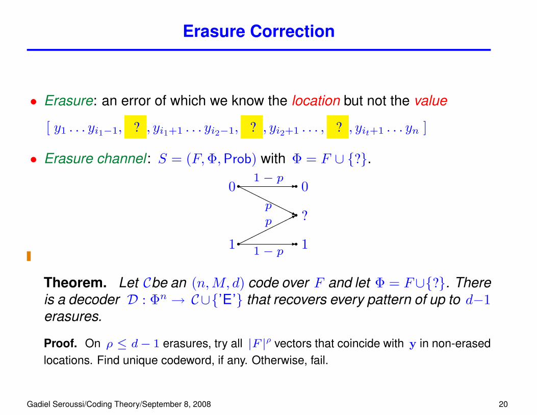
• Erasure: an error of which we know the location but not the value
[ y1 . . . yi1−1, ? , yi1+1 . . . yi2−1, ? , yi2+1 . . . , ? , yit+1 . . . yn ]
• Erasure channel : S = (F,Φ,Prob) with Φ = F ∪ {?}.
1 s
0 s
s 1s ?s 0
-
1− p
-1− p
����
�����*p
HHHHH
HHHHjp
Theorem. Let Cbe an (n,M, d) code over F and let Φ = F∪{?}. Thereis a decoder D : Φn → C∪{’E’} that recovers every pattern of up to d−1erasures.
Proof. On ρ ≤ d− 1 erasures, try all |F |ρ vectors that coincide with y in non-erasedlocations. Find unique codeword, if any. Otherwise, fail.
Gadiel Seroussi/Coding Theory/September 8, 2008 20
Combined correction/erasure/detection
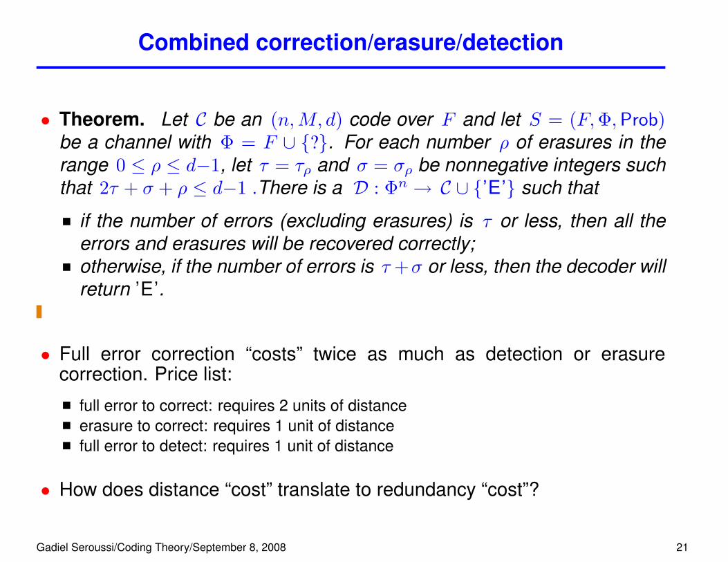
• Theorem. Let C be an (n,M, d) code over F and let S = (F,Φ,Prob)be a channel with Φ = F ∪ {?}. For each number ρ of erasures in therange 0 ≤ ρ ≤ d−1, let τ = τρ and σ = σρ be nonnegative integers suchthat 2τ + σ + ρ ≤ d−1 .There is a D : Φn → C ∪ {’E’} such that
if the number of errors (excluding erasures) is τ or less, then all theerrors and erasures will be recovered correctly;otherwise, if the number of errors is τ +σ or less, then the decoder willreturn ’E’.
• Full error correction “costs” twice as much as detection or erasurecorrection. Price list:
full error to correct: requires 2 units of distanceerasure to correct: requires 1 unit of distancefull error to detect: requires 1 unit of distance
• How does distance “cost” translate to redundancy “cost”?
Gadiel Seroussi/Coding Theory/September 8, 2008 21
Summary
-
u∈MChannelEncoder
-
c∈CChannel -
y∈ΦnChannelDecoder
-
c, u
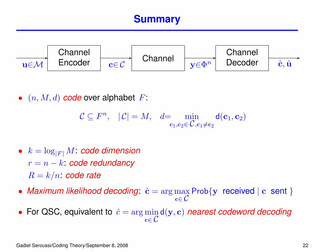
• (n,M, d) code over alphabet F :
C ⊆ Fn, | C| = M, d= minc1,c2∈ C,c1 6=c2
d(c1, c2)
• k = log|F |M : code dimensionr = n− k: code redundancyR = k/n: code rate
• Maximum likelihood decoding: c = arg maxc∈ C
Prob{y received | c sent }
• For QSC, equivalent to c = arg minc∈ C
d(y, c) nearest codeword decoding
Gadiel Seroussi/Coding Theory/September 8, 2008 22
Summary
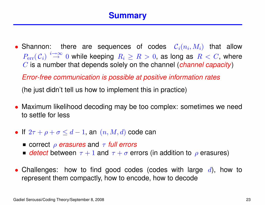
• Shannon: there are sequences of codes Ci(ni,Mi) that allowPerr( Ci)
i→∞→ 0 while keeping Ri ≥ R > 0, as long as R < C, whereC is a number that depends solely on the channel (channel capacity )
Error-free communication is possible at positive information rates
(he just didn’t tell us how to implement this in practice)
• Maximum likelihood decoding may be too complex: sometimes we needto settle for less
• If 2τ + ρ+ σ ≤ d− 1, an (n,M, d) code can
correct ρ erasures and τ full errorsdetect between τ + 1 and τ + σ errors (in addition to ρ erasures)
• Challenges: how to find good codes (codes with large d), how torepresent them compactly, how to encode, how to decode
Gadiel Seroussi/Coding Theory/September 8, 2008 23
2. Linear Codes
Gadiel Seroussi/Coding Theory/September 8, 2008 24

Linear Codes
• Assume F can be given a finite (or Galois) field structure
|F| = q, where q = pm for some prime number p and integer m ≥ 1. We denotesuch a field by Fq or GF(q)
Example: F2 with XOR, AND operations
• C : (n,M, d) over Fq is called linear if C is a linear sub-space of Fn overF
c1, c2 ∈ C, a1, a2 ∈ F ⇒ a1c1 + a2c2 ∈ C
• A linear code C has M = qk codewords, where k = logqM is thedimension of C as a linear space over F
• r = n− k is the redundancy of C, R = k/n its rate
• We use the notation [n, k, d] to denote the parameters of a linear code
Gadiel Seroussi/Coding Theory/September 8, 2008 25
Generator Matrix
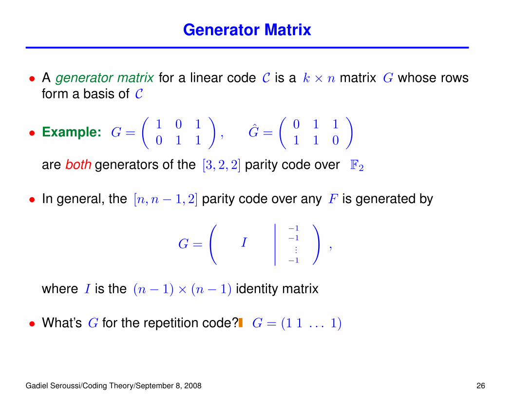
• A generator matrix for a linear code C is a k × n matrix G whose rowsform a basis of C
• Example: G =(
1 0 10 1 1
), G =
(0 1 11 1 0
)are both generators of the [3, 2, 2] parity code over F2
• In general, the [n, n− 1, 2] parity code over any F is generated by
G =
(I
−1−1
...−1
),
where I is the (n− 1)× (n− 1) identity matrix
• What’s G for the repetition code? G = (1 1 . . . 1)
Gadiel Seroussi/Coding Theory/September 8, 2008 26

Minimum Weight
• For an [n, k, d] code C,
c1, c2 ∈ C =⇒ c1 − c2 ∈ C , and d(c1, c2) = wt(c1 − c2) .
Therefore,
d = minc1,c2∈ C : c1 6=c2
d(c1, c2) = minc1,c2∈ C : c1 6=c2
wt(c1 − c2) = minc∈ C\{0}
wt(c) .
⇒ minimum distance is the same as minimum weight for linear codes
Recall also that 0 ∈ C and d(c, 0) = wt(c)
Gadiel Seroussi/Coding Theory/September 8, 2008 27
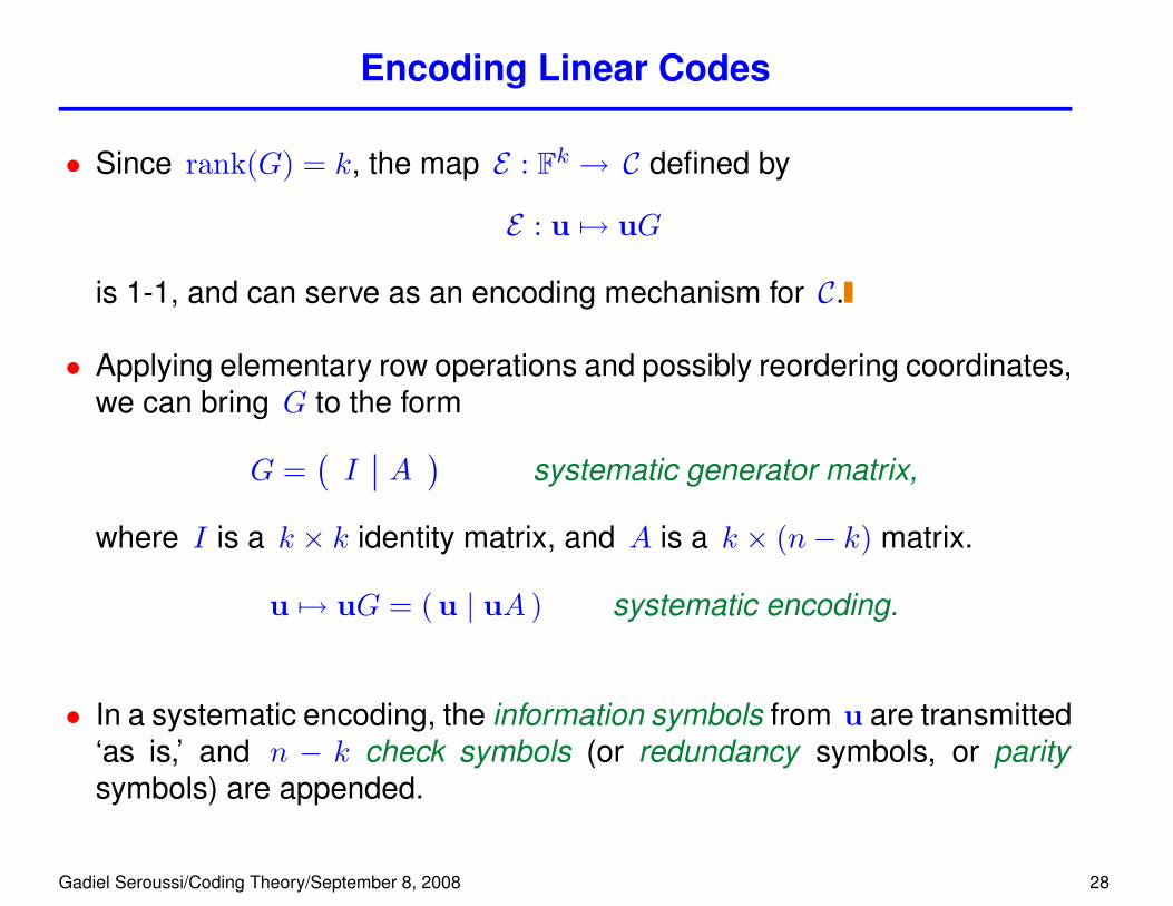
Encoding Linear Codes
• Since rank(G) = k, the map E : Fk → C defined by
E : u 7→ uG
is 1-1, and can serve as an encoding mechanism for C.
• Applying elementary row operations and possibly reordering coordinates,we can bring G to the form
G =(I A
)systematic generator matrix,
where I is a k × k identity matrix, and A is a k × (n− k) matrix.
u 7→ uG = ( u | uA ) systematic encoding.
• In a systematic encoding, the information symbols from u are transmitted‘as is,’ and n − k check symbols (or redundancy symbols, or paritysymbols) are appended.
Gadiel Seroussi/Coding Theory/September 8, 2008 28
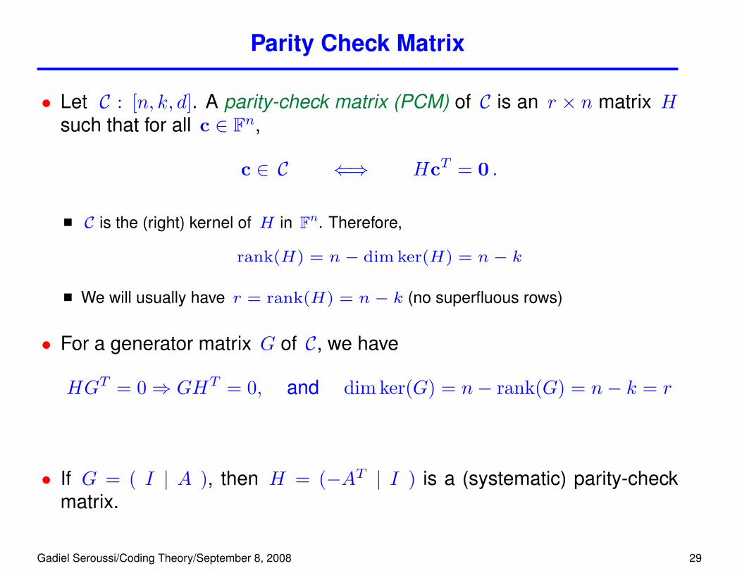
Parity Check Matrix
• Let C : [n, k, d]. A parity-check matrix (PCM) of C is an r × n matrix Hsuch that for all c ∈ Fn,
c ∈ C ⇐⇒ HcT = 0 .
C is the (right) kernel of H in Fn. Therefore,
rank(H) = n− dim ker(H) = n− k
We will usually have r = rank(H) = n− k (no superfluous rows)
• For a generator matrix G of C, we have
HGT = 0⇒ GHT = 0, and dim ker(G) = n− rank(G) = n− k = r
• If G = ( I | A ), then H = (−AT | I ) is a (systematic) parity-checkmatrix.
Gadiel Seroussi/Coding Theory/September 8, 2008 29

Dual Code
• The dual code of C : [n, k, d] is
C⊥ = {x ∈ Fn : xcT = 0 ∀c ∈ C },
or, equivalentlyC⊥ = {x ∈ Fn : xGT = 0 }.
• ( C⊥)⊥ = C
• G and H of C reverse roles for C⊥:
C :{G = H⊥
H = G⊥
}: C⊥ .
• C⊥ is an [n, n− k, d⊥] code over F
Gadiel Seroussi/Coding Theory/September 8, 2008 30

Examples
• H = ( 1 1 . . . 1 ) is a PCM for the [n, n − 1, 2] parity code, which hasgenerator matrix
G =
(I
−1−1
...−1
).
On the other hand, H generates the [n, 1, n] repetition code, and G is acheck matrix for it ⇒ parity and repetition codes are dual .
• [7, 4, 3] Hamming code over F2 is defined by
H =
0@ 0 0 0 1 1 1 10 1 1 0 0 1 11 0 1 0 1 0 1
1A , G =
0BB@1 1 1 1 1 1 10 0 0 1 1 1 10 1 1 0 0 1 11 0 1 0 1 0 1
1CCA .
• GHT = 0 can be verified by direct inspection
Gadiel Seroussi/Coding Theory/September 8, 2008 31
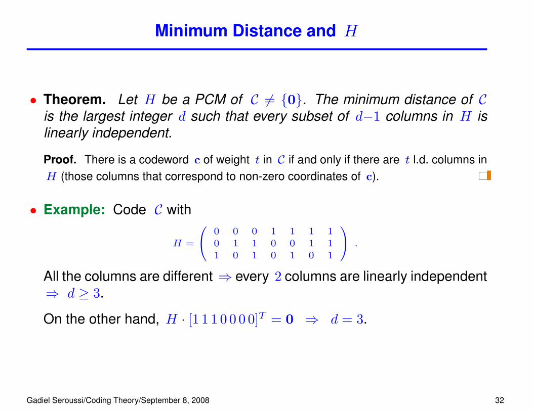
Minimum Distance and H
• Theorem. Let H be a PCM of C 6= {0}. The minimum distance of Cis the largest integer d such that every subset of d−1 columns in H islinearly independent.
Proof. There is a codeword c of weight t in C if and only if there are t l.d. columns inH (those columns that correspond to non-zero coordinates of c).
• Example: Code C with
H =
0@ 0 0 0 1 1 1 10 1 1 0 0 1 11 0 1 0 1 0 1
1A .
All the columns are different ⇒ every 2 columns are linearly independent⇒ d ≥ 3.
On the other hand, H · [1 1 1 0 0 0 0]T = 0 ⇒ d = 3.
Gadiel Seroussi/Coding Theory/September 8, 2008 32
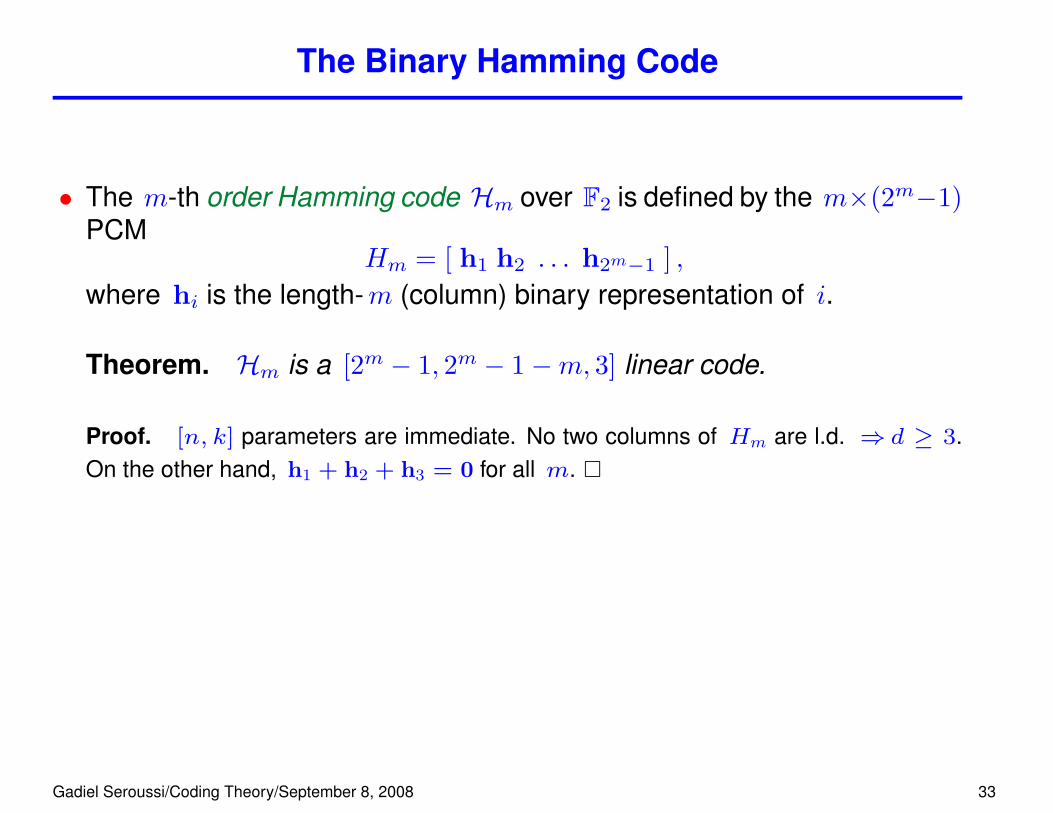
The Binary Hamming Code
• The m-th order Hamming code Hm over F2 is defined by the m×(2m−1)PCM
Hm = [ h1 h2 . . . h2m−1 ] ,where hi is the length-m (column) binary representation of i.
Theorem. Hm is a [2m − 1, 2m − 1−m, 3] linear code.
Proof. [n, k] parameters are immediate. No two columns of Hm are l.d. ⇒ d ≥ 3.On the other hand, h1 + h2 + h3 = 0 for all m. �
Gadiel Seroussi/Coding Theory/September 8, 2008 33
The q-ary Hamming Code
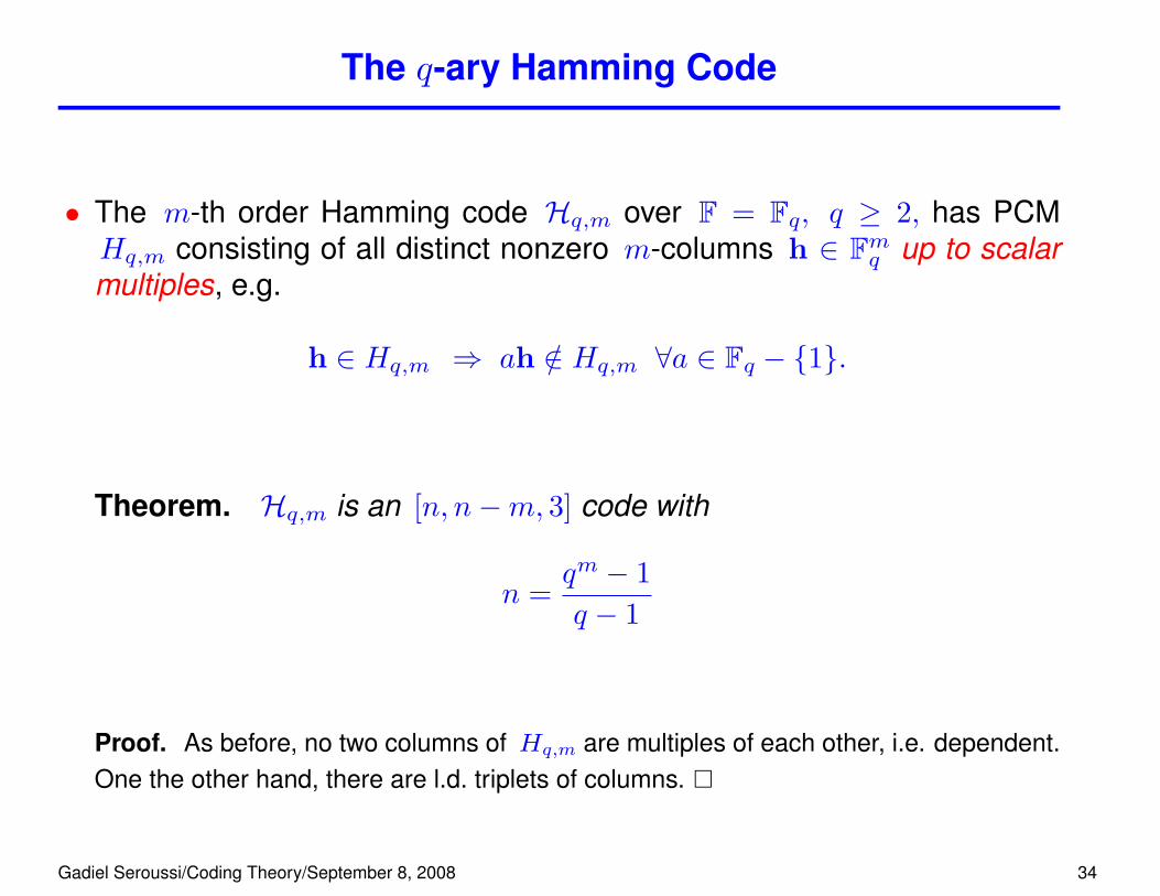
• The m-th order Hamming code Hq,m over F = Fq, q ≥ 2, has PCMHq,m consisting of all distinct nonzero m-columns h ∈ Fmq up to scalarmultiples, e.g.
h ∈ Hq,m ⇒ ah /∈ Hq,m ∀a ∈ Fq − {1}.
Theorem. Hq,m is an [n, n−m, 3] code with
n =qm − 1q − 1
Proof. As before, no two columns of Hq,m are multiples of each other, i.e. dependent.One the other hand, there are l.d. triplets of columns. �
Gadiel Seroussi/Coding Theory/September 8, 2008 34
Cosets and Syndromes
• Let y ∈ Fn. The syndrome of y (with respect to a PCM H of C) isdefined by
s = HyT ∈ Fn−k.The set
y + C = {y + c : c ∈ C}is a coset of C (as an additive subgroup) in Fn.
• If y1 ∈ y + C, then
y1 − y ∈ C ⇒ H(y1 − y)T = 0 ⇒ HyT1 = HyT
⇒ The syndrome is invariant for all y1 ∈ y + C.
• Let F = Fq. Given a PCM H, there is a 1-1 correspondence betweenthe qn−k cosets of C in Fn and the qn−k possible syndrome values (His full-rank ⇒ all values are attained).
Gadiel Seroussi/Coding Theory/September 8, 2008 35

Syndrome Decoding of Linear Codes
• c ∈ C is sent and y = c + e is received on an additive channel
• y and e are in the same coset of C
• Nearest-neighbor decoding of y calls for finding the closest codeword cto y ⇒ find a vector e of lowest weight in y+ C: a coset leader .
coset leaders need not be unique (when are they?)
• Decoding algorithm: upon receiving y
compute the syndrome s = HyT
find a coset leader e in the coset corresponding to sdecode y into c = y − e
• If n − k is (very) small, a table containing one leader per coset can bepre-computed. The table is indexed by s.
• In general, however, syndrome decoding appears exponential in n − k.In fact, it has been shown to be NP-hard.
Gadiel Seroussi/Coding Theory/September 8, 2008 36
Decoding the Hamming Code
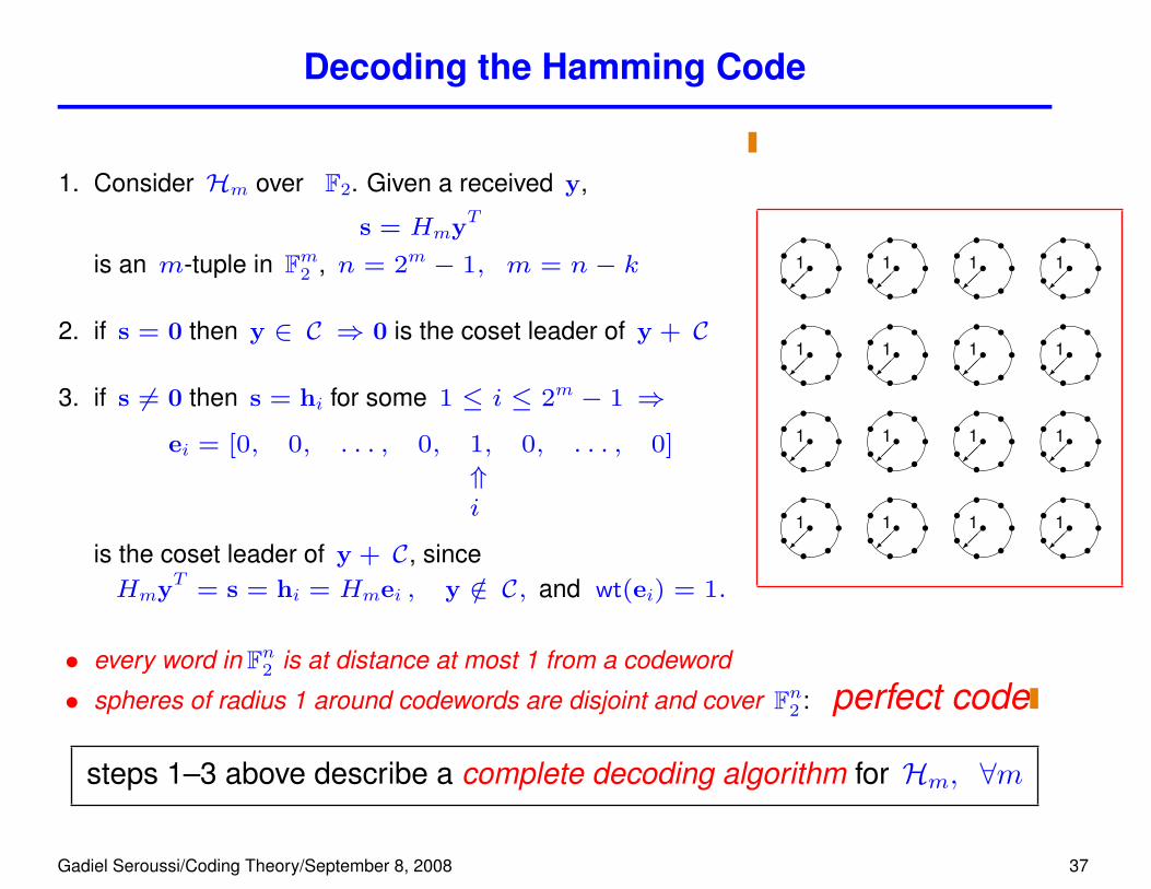
1. Consider Hm over F2. Given a received y,
s = HmyT
is an m-tuple in Fm2 , n = 2m − 1, m = n− k
2. if s = 0 then y ∈ C ⇒ 0 is the coset leader of y + C
3. if s 6= 0 then s = hi for some 1 ≤ i ≤ 2m − 1 ⇒
ei = [0, 0, . . . , 0, 1, 0, . . . , 0]
⇑i
is the coset leader of y + C, sinceHmyT = s = hi = Hmei , y /∈ C, and wt(ei) = 1.
&%'$sssss s ss��1 &%'$sssss s ss��1 &%'$sssss s ss��1 &%'$sssss s ss��1
&%'$sssss s ss��1 &%'$sssss s ss��1 &%'$sssss s ss��1 &%'$sssss s ss��1
&%'$sssss s ss��1 &%'$sssss s ss��1 &%'$sssss s ss��1 &%'$sssss s ss��1
&%'$sssss s ss��1 &%'$sssss s ss��1 &%'$sssss s ss��1 &%'$sssss s ss��1
• every word in Fn2 is at distance at most 1 from a codeword
• spheres of radius 1 around codewords are disjoint and cover Fn2 : perfect code
steps 1–3 above describe a complete decoding algorithm for Hm, ∀m
Gadiel Seroussi/Coding Theory/September 8, 2008 37

Deriving Codes from Other Codes
• Adding an overall parity check. Let C be an [n, k, d] code with some odd-weight codewords. We form a new code C by appending a 0 at the endof even-weight codewords, and a 1 at the end of odd-weight ones.C is an [n+ 1, k, d+ 1] code. Every codeword in C has even weight.
Example: The [7, 4, 3] binary Hamming code can be extended to an [8, 4, 4] codewith PCM
H =
0BB@0 0 0 1 1 1 1 0
0 1 1 0 0 1 1 0
1 0 1 0 1 0 1 0
1 1 1 1 1 1 1 1
1CCA corrects any pattern of 1 error, anddetects any pattern of 2.
• Expurgate by throwing away codewords. E.g., select subset ofcodewords satisfying an independent parity check.
Example: Selecting the even-weight sub-code of the [2m − 1, 2m − 1 − m, 3]
Hamming code yields a [2m − 1, 2m − 2−m, 4] code.
• Shortening by taking a cross-section. Select all codewords c with,say, c1 = 0, and eliminate that coordinate (can be repeated for morecoordinates). An [n, k, d] code yields an [n− 1, k − 1,≥ d] code.
Gadiel Seroussi/Coding Theory/September 8, 2008 38
3. Bounds on Code Parameters
Gadiel Seroussi/Coding Theory/September 8, 2008 39

The Singleton Bound
• The Singleton bound .
Theorem. For any (n,M, d) code over an alphabet of size q,
d ≤ n− (logqM) + 1 .
Proof. Let ` = dlogqMe − 1. Since q` < M , there must be at least two codewordsthat agree in their first ` coordinates. Hence, d ≤ n− `. �
• For linear codes, we have d ≤ n = k + 1.
• C : (n,M, d) is called maximum distance separable (MDS) if it meets theSingleton bound, namely d = n− (logqM) + 1.
Gadiel Seroussi/Coding Theory/September 8, 2008 40

MDS Code Examples
• Trivial and semi-trivial codes
[n, n, 1] whole space Fnq , [n, n− 1, 2] parity code, [n, 1, n] repetition code
• Normalized generalized Reed-Solomon (RS) codes
Let α1, α2, . . . , αn be distinct elements of Fq, n ≤ q. The RS code hasPCM
HRS =
1 1 . . . 1α1 α2 . . . αnα2
1 α22 . . . α2
n... ... ... ...αn−k−1
1 αn−k−12 . . . αn−k−1
n
.
Theorem. Every Reed-Solomon code is MDS.
Proof. Every (n−k) × (n−k) sub-matrix of HRS has a nonsingular Vandermondeform. Hence, every (n−k) columns of HRS are l.i. ⇒d ≥ n− k + 1. �
Gadiel Seroussi/Coding Theory/September 8, 2008 41
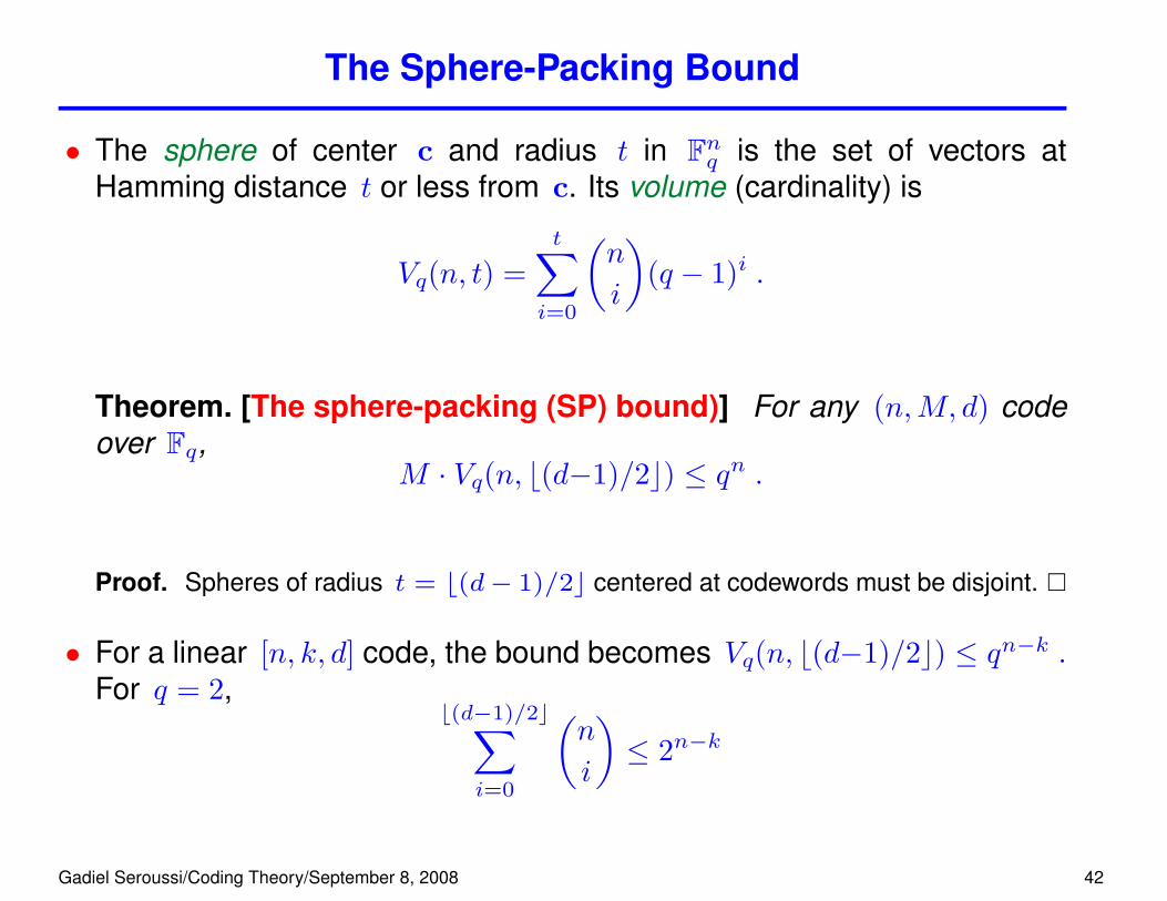
The Sphere-Packing Bound
• The sphere of center c and radius t in Fnq is the set of vectors atHamming distance t or less from c. Its volume (cardinality) is
Vq(n, t) =t∑i=0
(n
i
)(q − 1)i .
Theorem. [The sphere-packing (SP) bound)] For any (n,M, d) codeover Fq,
M · Vq(n, b(d−1)/2c) ≤ qn .
Proof. Spheres of radius t = b(d− 1)/2c centered at codewords must be disjoint. �
• For a linear [n, k, d] code, the bound becomes Vq(n, b(d−1)/2c) ≤ qn−k .For q = 2,
b(d−1)/2c∑i=0
(n
i
)≤ 2n−k
Gadiel Seroussi/Coding Theory/September 8, 2008 42
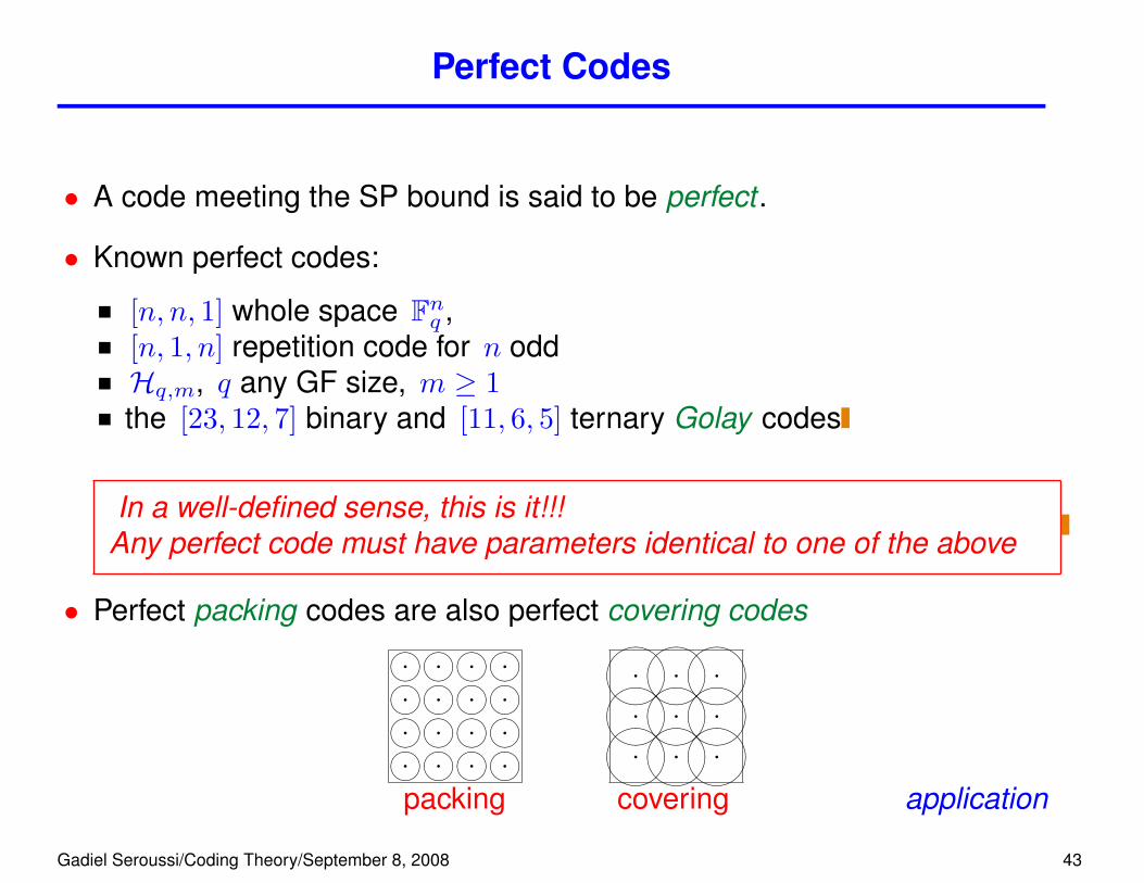
Perfect Codes
• A code meeting the SP bound is said to be perfect .
• Known perfect codes:
[n, n, 1] whole space Fnq ,[n, 1, n] repetition code for n oddHq,m, q any GF size, m ≥ 1the [23, 12, 7] binary and [11, 6, 5] ternary Golay codes
In a well-defined sense, this is it!!!Any perfect code must have parameters identical to one of the above
• Perfect packing codes are also perfect covering codes
����q ����q ����q ����q����q ����q ����q ����q����q ����q ����q ����q����q ����q ����q ����q
q&%'$q&%'$q&%'$q
&%'$q&%'$q&%'$q
&%'$q&%'$q&%'$
packing covering application
Gadiel Seroussi/Coding Theory/September 8, 2008 43

The Gilbert-Varshamov bound
• The Singleton and SP bounds set necessary conditions on theparameters of a code. The following is a sufficient condition:
Theorem. [The Gilbert-Varshamov (GV) bound] There exists an [n, k, d]code over the field Fq whenever
Vq(n−1, d−2) < qn−k.
Proof. Construct, iteratively, an (n − k) × n PCM where every d − 1 columns arel.i., starting with an identity matrix, and adding a new column in each iteration. Assumewe’ve gotten `−1 columns. There are at most Vq(n−1, d−2) linear combinations ofd − 2 or less of these columns. As long as Vq(`−1, d−2) < qn−k , we can find acolumn we can add without creating a dependence of d− 1 columns.�
Theorem. Let
ρ =qk − 1q − 1
· Vq(n, d−1)qn
.
Then, a random [n, k] code has minimum distance d with Prob ≥ 1− ρ.
Lots of codes are near the GV bound. But it’s very hard to find them!
Gadiel Seroussi/Coding Theory/September 8, 2008 44

Asymptotic Bounds
• Def.: relative distance δ = d/n
• We are interested in the behavior of δ and R = logqM as n→∞.
• Singleton bound: d ≤ n− dlogqMe+ 1 ⇒ R ≤ 1− δ + o(1)
• For the SP and GV bounds, we need estimates for Vq(n, t)
• Def.: symmetric q-ary entropy function Hq : [0, 1]→ [0, 1]
Hq(x) = −x logq x− (1− x) logq(1− x) + x logq(q−1) ,
Hq(0) = 0, Hq(1) = logq(q − 1), strictly ∩-convex, max = 1 at x = 1− 1/q
coincides with H(x) when q = 2
Gadiel Seroussi/Coding Theory/September 8, 2008 45

Asymptotic Bounds (II)
Lemma. For 0 ≤ t/n ≤ 1− (1/q),
Vq(n, t) =
tXi=0
“ni
”(q − 1)
i ≤ qnHq(t/n).
Lemma. For integers 0 ≤ t ≤ n,
Vq(n, t) ≥“nt
”(q − 1)
t ≥1p
8t(1− (t/n))· qnHq(t/n)
.
Theorem. [Asymptotic SP bound] For every (n, qnR, δn) code over Fq,
R ≤ 1−Hq(δ/2)+o(1) .
Theorem. [Asymptotic GV bound] Let n, nR, δn be positive integerssuch that δ ∈ (0, 1−(1/q)] and
R ≤ 1− Hq(δ) .
Then, there exists a linear [n, nR,≥δn] code over Fq.
Gadiel Seroussi/Coding Theory/September 8, 2008 46
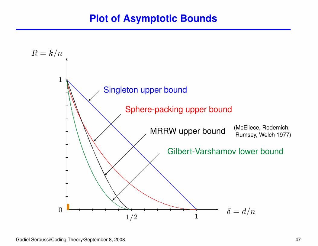
Plot of Asymptotic Bounds
-
6
R = k/n
0
1
1/2 1δ = d/n
���
Singleton upper bound@@@@@@@@@@@@@@@@@@@@@@@@@@@@@@@@@
��
��
���
Sphere-packing upper bound
���
���
��
����
Gilbert-Varshamov lower bound
��
��
���
����
MRRW upper bound (McEliece, Rodemich,Rumsey, Welch 1977)
Gadiel Seroussi/Coding Theory/September 8, 2008 47

4. Brief Review of Finite Fields
Gadiel Seroussi/Coding Theory/September 8, 2008 48
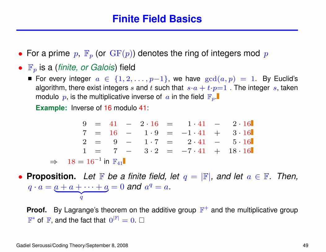
Finite Field Basics
• For a prime p, Fp (or GF(p)) denotes the ring of integers mod p
• Fp is a (finite, or Galois) fieldFor every integer a ∈ {1, 2, . . . , p−1}, we have gcd(a, p) = 1. By Euclid’salgorithm, there exist integers s and t such that s·a+ t·p=1 . The integer s, takenmodulo p, is the multiplicative inverse of a in the field Fp.Example: Inverse of 16 modulo 41:
9 = 41 − 2 · 16 = 1 · 41 − 2 · 16
7 = 16 − 1 · 9 = −1 · 41 + 3 · 16
2 = 9 − 1 · 7 = 2 · 41 − 5 · 16
1 = 7 − 3 · 2 = −7 · 41 + 18 · 16
⇒ 18 = 16−1 in F41
• Proposition. Let F be a finite field, let q = |F|, and let a ∈ F. Then,q · a = a+ a+ · · ·+ a︸ ︷︷ ︸
q
= 0 and aq = a.
Proof. By Lagrange’s theorem on the additive group F+ and the multiplicative groupF∗ of F, and the fact that 0|F| = 0. �
Gadiel Seroussi/Coding Theory/September 8, 2008 49
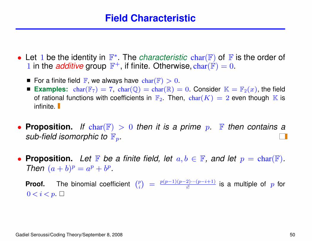
Field Characteristic
• Let 1 be the identity in F∗. The characteristic char(F) of F is the order of1 in the additive group F+, if finite. Otherwise, char(F) = 0.
For a finite field F, we always have char(F) > 0.Examples: char(F7) = 7, char(Q) = char(R) = 0. Consider K = F2(x), the fieldof rational functions with coefficients in F2. Then, char(K) = 2 even though K isinfinite.
• Proposition. If char(F) > 0 then it is a prime p. F then contains asub-field isomorphic to Fp.
• Proposition. Let F be a finite field, let a, b ∈ F, and let p = char(F).Then (a+ b)p = ap + bp.
Proof. The binomial coefficient`pi
´= p(p−1)(p−2)···(p−i+1)
i! is a multiple of p for0< i<p. �
Gadiel Seroussi/Coding Theory/September 8, 2008 50
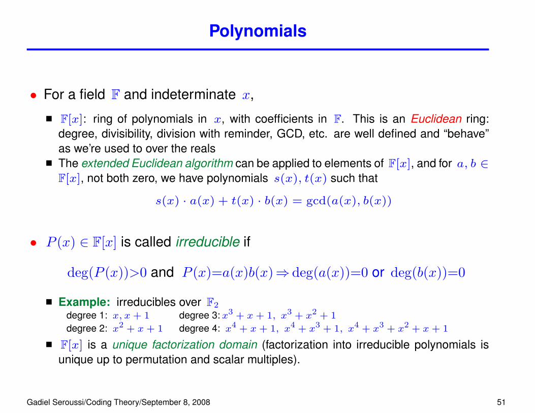
Polynomials
• For a field F and indeterminate x,
F[x]: ring of polynomials in x, with coefficients in F. This is an Euclidean ring:degree, divisibility, division with reminder, GCD, etc. are well defined and “behave”as we’re used to over the realsThe extended Euclidean algorithm can be applied to elements of F[x], and for a, b ∈F[x], not both zero, we have polynomials s(x), t(x) such that
s(x) · a(x) + t(x) · b(x) = gcd(a(x), b(x))
• P (x) ∈ F[x] is called irreducible if
deg(P (x))>0 and P (x)=a(x)b(x)⇒ deg(a(x))=0 or deg(b(x))=0
Example: irreducibles over F2
degree 1: x, x+ 1 degree 3: x3 + x+ 1, x3 + x2 + 1
degree 2: x2 + x+ 1 degree 4: x4 + x+ 1, x4 + x3 + 1, x4 + x3 + x2 + x+ 1
F[x] is a unique factorization domain (factorization into irreducible polynomials isunique up to permutation and scalar multiples).
Gadiel Seroussi/Coding Theory/September 8, 2008 51
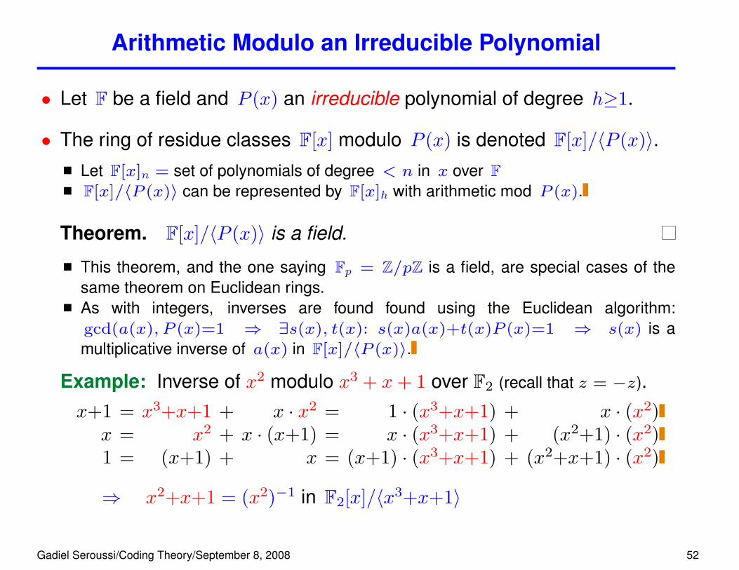
Arithmetic Modulo an Irreducible Polynomial
• Let F be a field and P (x) an irreducible polynomial of degree h≥1.
• The ring of residue classes F[x] modulo P (x) is denoted F[x]/〈P (x)〉.Let F[x]n = set of polynomials of degree < n in x over FF[x]/〈P (x)〉 can be represented by F[x]h with arithmetic mod P (x).
Theorem. F[x]/〈P (x)〉 is a field.
This theorem, and the one saying Fp = Z/pZ is a field, are special cases of thesame theorem on Euclidean rings.As with integers, inverses are found found using the Euclidean algorithm:gcd(a(x), P (x)=1 ⇒ ∃s(x), t(x): s(x)a(x)+t(x)P (x)=1 ⇒ s(x) is amultiplicative inverse of a(x) in F[x]/〈P (x)〉.
Example: Inverse of x2 modulo x3 + x+ 1 over F2 (recall that z = −z).x+1 = x3+x+1 + x · x2 = 1 · (x3+x+1) + x · (x2)x = x2 + x · (x+1) = x · (x3+x+1) + (x2+1) · (x2)1 = (x+1) + x = (x+1) · (x3+x+1) + (x2+x+1) · (x2)
⇒ x2+x+1 = (x2)−1 in F2[x]/〈x3+x+1〉
Gadiel Seroussi/Coding Theory/September 8, 2008 52

Extension Fields
• A field K is an extension field of a field F if F is a sub-field of K
• K is a vector space over F. The dimension [K : F] of this vector spaceis referred to as the extension degree of K over F.
If [K : F] is finite, K is called a finite extension of F . A finite extensionis not necessarily a finite field: C is a finite extension of R.
F[x]/〈P (x)〉 is an extension of degree h of F, where h = deg(P ).
When Fq is a finite field with q elements, F[x]/〈P (x)〉 has qh elements.
If |F| = q, and char(F) = p, then q = pm for some integer m ≥ 1.
Gadiel Seroussi/Coding Theory/September 8, 2008 53
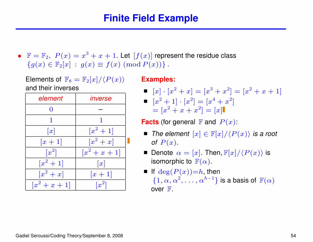
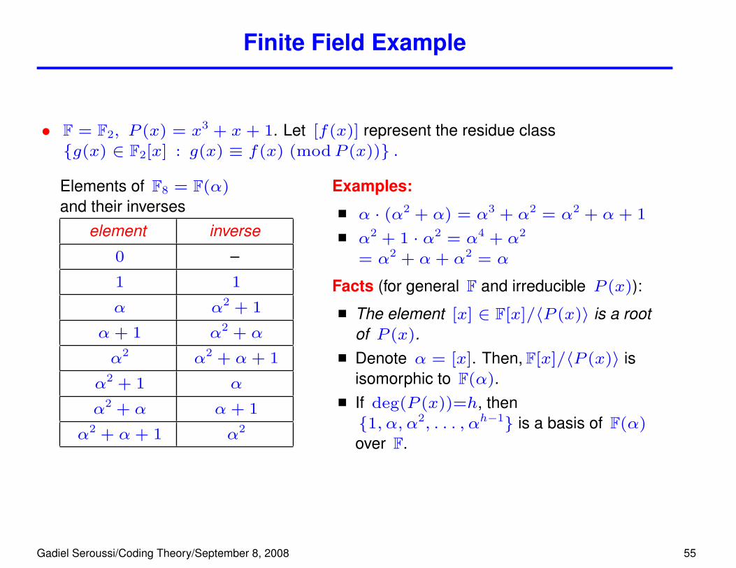
Finite Field Example
• F = F2, P (x) = x3 + x+ 1. Let [f(x)] represent the residue class{g(x) ∈ F2[x] : g(x) ≡ f(x) (modP (x))} .
Elements of F8 = F2[x]/〈P (x)〉and their inverses
element inverse
0 –
1 1
[x] [x2 + 1]
[x+ 1] [x2 + x]
[x2] [x2 + x+ 1]
[x2 + 1] [x]
[x2 + x] [x+ 1]
[x2 + x+ 1] [x2]
Examples:
[x] · [x2 + x] = [x3 + x2] = [x2 + x+ 1]
[x2 + 1] · [x2] = [x4 + x2]
= [x2 + x+ x2] = [x]
Facts (for general F and P (x):
The element [x] ∈ F[x]/〈P (x)〉 is a rootof P (x).Denote α = [x]. Then, F[x]/〈P (x)〉 isisomorphic to F(α).If deg(P (x))=h, then{1, α, α2, . . . , αh−1} is a basis of F(α)
over F.
Gadiel Seroussi/Coding Theory/September 8, 2008 54
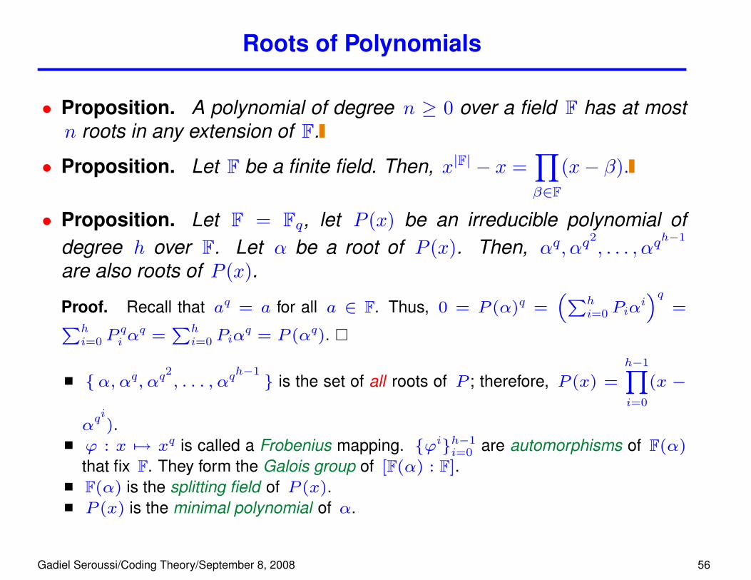
Finite Field Example
• F = F2, P (x) = x3 + x+ 1. Let [f(x)] represent the residue class{g(x) ∈ F2[x] : g(x) ≡ f(x) (modP (x))} .
Elements of F8 = F(α)
and their inverseselement inverse
0 –
1 1
α α2 + 1
α+ 1 α2 + α
α2 α2 + α+ 1
α2 + 1 α
α2 + α α+ 1
α2 + α+ 1 α2
Examples:
α · (α2 + α) = α3 + α2 = α2 + α+ 1
α2 + 1 · α2 = α4 + α2
= α2 + α+ α2 = α
Facts (for general F and irreducible P (x)):
The element [x] ∈ F[x]/〈P (x)〉 is a rootof P (x).Denote α = [x]. Then, F[x]/〈P (x)〉 isisomorphic to F(α).If deg(P (x))=h, then{1, α, α2, . . . , αh−1} is a basis of F(α)
over F.
Gadiel Seroussi/Coding Theory/September 8, 2008 55
Roots of Polynomials
• Proposition. A polynomial of degree n ≥ 0 over a field F has at mostn roots in any extension of F.
• Proposition. Let F be a finite field. Then, x|F| − x =∏β∈F
(x− β).
• Proposition. Let F = Fq, let P (x) be an irreducible polynomial ofdegree h over F. Let α be a root of P (x). Then, αq, αq
2, . . . , αq
h−1
are also roots of P (x).
Proof. Recall that aq = a for all a ∈ F. Thus, 0 = P (α)q =“Ph
i=0 Piαi”q
=Phi=0 P
qi α
q =Ph
i=0 Piαq = P (αq). �
{α, αq, αq2, . . . , αq
h−1} is the set of all roots of P ; therefore, P (x) =
h−1Yi=0
(x −
αqi
).ϕ : x 7→ xq is called a Frobenius mapping. {ϕi}h−1
i=0 are automorphisms of F(α)
that fix F. They form the Galois group of [F(α) : F].F(α) is the splitting field of P (x).P (x) is the minimal polynomial of α.
Gadiel Seroussi/Coding Theory/September 8, 2008 56
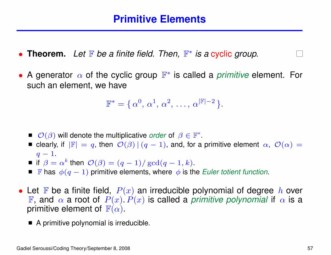
Primitive Elements
• Theorem. Let F be a finite field. Then, F∗ is a cyclic group.
• A generator α of the cyclic group F∗ is called a primitive element. Forsuch an element, we have
F∗ = {α0, α1, α2, . . . , α|F|−2 }.
O(β) will denote the multiplicative order of β ∈ F∗.clearly, if |F| = q, then O(β) | (q − 1), and, for a primitive element α, O(α) =
q − 1.if β = αk then O(β) = (q − 1)/ gcd(q − 1, k).F has φ(q − 1) primitive elements, where φ is the Euler totient function.
• Let F be a finite field, P (x) an irreducible polynomial of degree h overF, and α a root of P (x).P (x) is called a primitive polynomial if α is aprimitive element of F(α).
A primitive polynomial is irreducible.
Gadiel Seroussi/Coding Theory/September 8, 2008 57
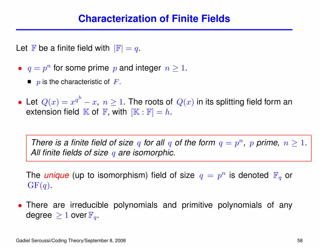
Characterization of Finite Fields
Let F be a finite field with |F| = q.
• q = pn for some prime p and integer n ≥ 1.
p is the characteristic of F .
• Let Q(x) = xqh − x, n ≥ 1. The roots of Q(x) in its splitting field form an
extension field K of F, with [K : F] = h.
There is a finite field of size q for all q of the form q = pn, p prime, n ≥ 1.All finite fields of size q are isomorphic.
The unique (up to isomorphism) field of size q = pn is denoted Fq orGF(q).
• There are irreducible polynomials and primitive polynomials of anydegree ≥ 1 over Fq.
Gadiel Seroussi/Coding Theory/September 8, 2008 58
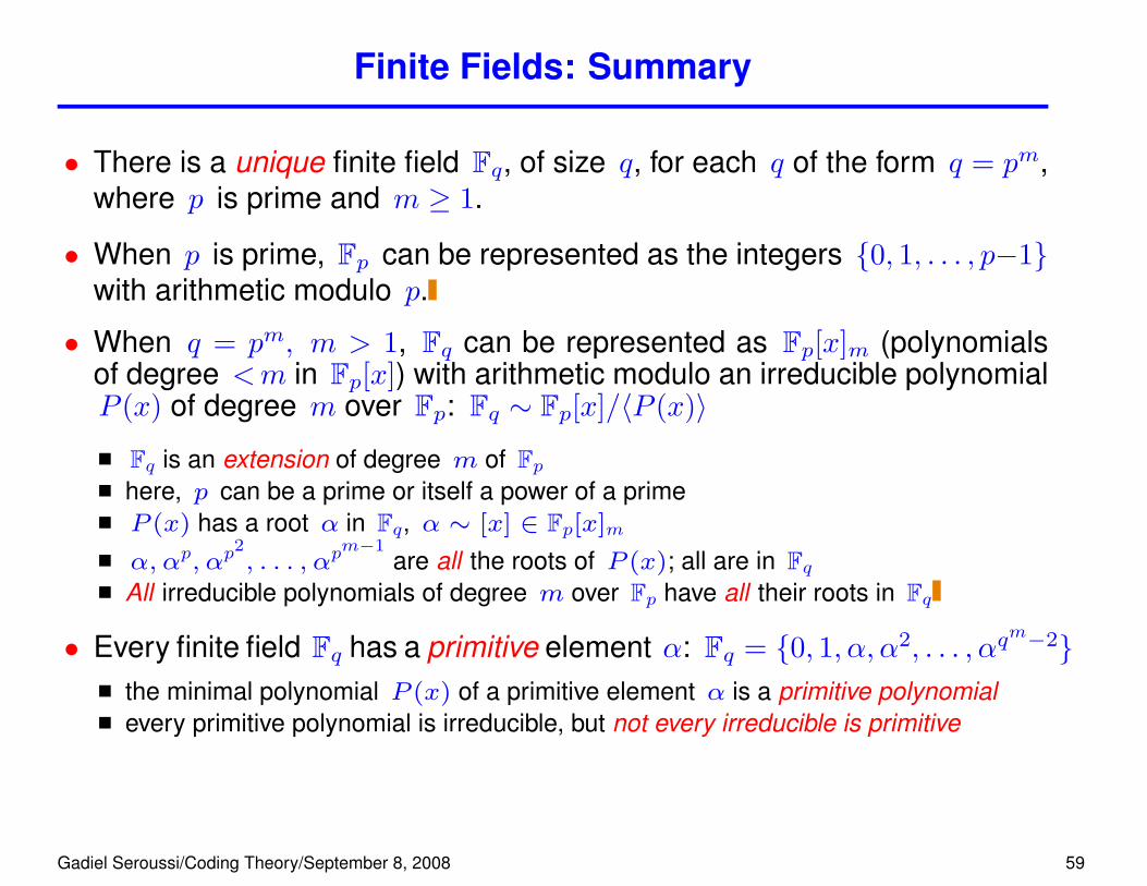
Finite Fields: Summary
• There is a unique finite field Fq, of size q, for each q of the form q = pm,where p is prime and m ≥ 1.
• When p is prime, Fp can be represented as the integers {0, 1, . . . , p−1}with arithmetic modulo p.
• When q = pm, m > 1, Fq can be represented as Fp[x]m (polynomialsof degree <m in Fp[x]) with arithmetic modulo an irreducible polynomialP (x) of degree m over Fp: Fq ∼ Fp[x]/〈P (x)〉
Fq is an extension of degree m of Fphere, p can be a prime or itself a power of a primeP (x) has a root α in Fq, α ∼ [x] ∈ Fp[x]m
α, αp, αp2, . . . , αp
m−1are all the roots of P (x); all are in Fq
All irreducible polynomials of degree m over Fp have all their roots in Fq
• Every finite field Fq has a primitive element α: Fq = {0, 1, α, α2, . . . , αqm−2}
the minimal polynomial P (x) of a primitive element α is a primitive polynomialevery primitive polynomial is irreducible, but not every irreducible is primitive
Gadiel Seroussi/Coding Theory/September 8, 2008 59

Finite Field Example: F16
α is a root of P (x) = x4 + x+ 1 ∈ F2[x] (primitive).
binaryi αi 0123 min poly– 0 0000 x
0 1 1000 x+ 1
1 α 0100 x4+x+1
2 α2 0010 x4+x+1
3 α3 0001 x4+x3+x2+x+1
4 α+ 1 1100 x4+x+1
5 α2 + α 0110 x2+x+1
6 α3 + α2 0011 x4+x3+x2+x+1
7 α3 + α+ 1 1101 x4+x3+1
8 α2 + 1 1010 x4+x+1
9 α3 + α 0101 x4+x3+x2+x+1
10 α2 + α+ 1 1110 x2+x+1
11 α3 + α2 + α 0111 x4+x3+1
12 α3 + α2 + α+ 1 1111 x4+x3+x2+x+1
13 α3 + α2 + 1 1011 x4+x3+1
14 α3 + 1 1001 x4+x3+1
• if β = αi, 0 ≤i ≤ (q − 2), we saythat i is the discretelogarithm of β to baseα.
Examples:• (α2+α)·(α3+α2) =
α5 ·α6 = α11 = α3 +
α2 + α
• (α3 + α + 1)−1 =
α−7 = α8 = α2 + 1
• logα(α3 + α2 + 1) =
13
Gadiel Seroussi/Coding Theory/September 8, 2008 60
The Number of Irreducible Polynomials
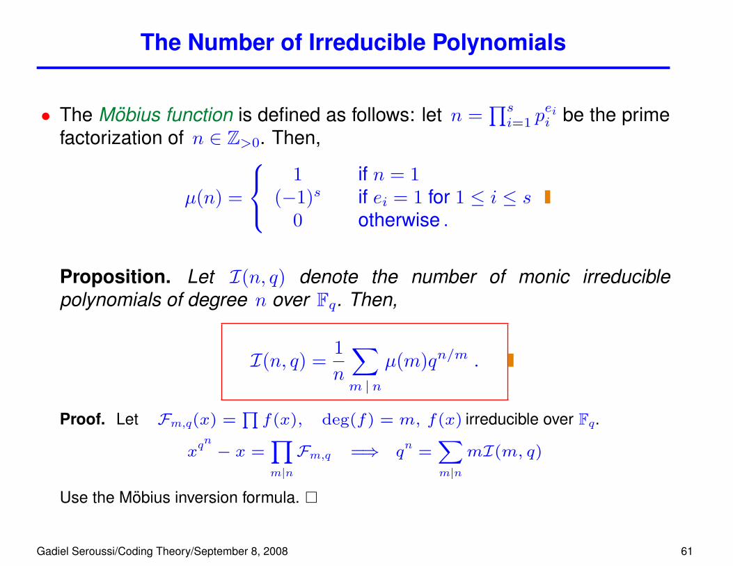
• The Mobius function is defined as follows: let n =∏si=1 p
eii be the prime
factorization of n ∈ Z>0. Then,
µ(n) =
1 if n = 1(−1)s if ei = 1 for 1 ≤ i ≤ s
0 otherwise .
Proposition. Let I(n, q) denote the number of monic irreduciblepolynomials of degree n over Fq. Then,
I(n, q) =1n
∑m |n
µ(m)qn/m .
Proof. Let Fm,q(x) =Qf(x), deg(f) = m, f(x) irreducible over Fq.
xqn − x =
Ym|n
Fm,q =⇒ qn
=Xm|n
mI(m, q)
Use the Mobius inversion formula. �
Gadiel Seroussi/Coding Theory/September 8, 2008 61

Application: Double-Error Correcting Codes
• We can rewrite the PCM of the [2m−1, 2m−1−m, 3] binary Hamming code Hm overF2 as
H = (α1 α2 . . . α2m−1 ) ,where αj ranges over all the nonzero elements of F2.
• Example: Let m=4 and α a root of P (x)=x4 + x+ 1. We take αj=αj−1, and
H4 =
0BB@1 0 0 0 1 0 0 1 1 0 1 0 1 1 1
0 1 0 0 1 1 0 1 0 1 1 1 1 0 0
0 0 1 0 0 1 1 0 1 0 1 1 1 1 0
0 0 0 1 0 0 1 1 0 1 0 1 1 1 1
1CCA .
• A vector c = (c1 c2 . . . cn) is a codeword of Hm iff
HmcT =
nXj=1
cjαj = 0.
• If there is exactly one error, the error vector is of the form ei = [0i−1 1 0n−i], and thesyndrome is s = HmeTi = αj. The syndrome gives us the error location directly.
Gadiel Seroussi/Coding Theory/September 8, 2008 62

Application: Double-Error Correcting Codes (II)
• What if there are two errors? Then, we get e = ei + ej, and
s = αi + αj, for some i, j, 1 ≤ i < j ≤ n,
which is insufficient to solve for αi, αj. We need more equations ...
• Consider the PCMHm =
„α1 α2 . . . α2m−1
α31 α3
2 . . . α32m−1
«.
Syndromes are of the form
s =
„s1
s3
«= HmyT = HmeT .
Assume that the number of errors is at most 2.
Case 1: e = 0 (no errors). Then, s1 = s3 = 0.Case 2: e = ei for some i, 1 ≤ i ≤ n (one error). Then,„
s1
s3
«= HmeT =
„αiα3i
«;
namely, s3 = s31 6= 0, and the error location is the index i such that αi = s1.
Gadiel Seroussi/Coding Theory/September 8, 2008 63
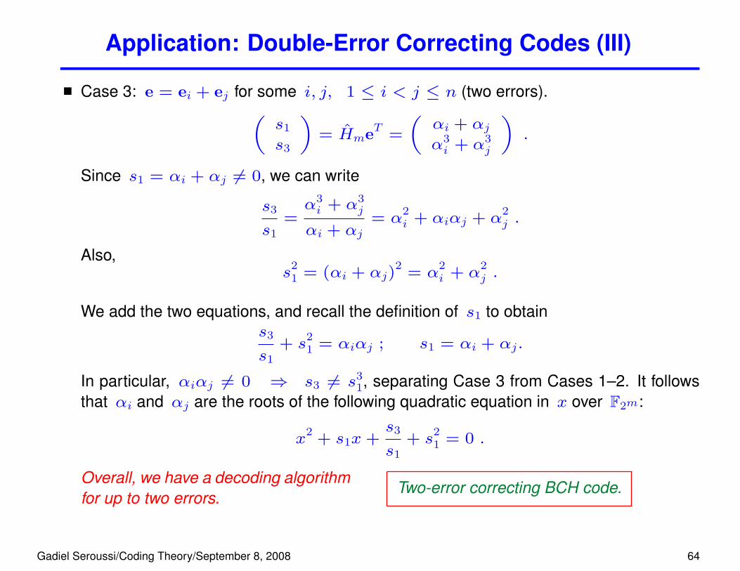
Application: Double-Error Correcting Codes (III)
Case 3: e = ei + ej for some i, j, 1 ≤ i < j ≤ n (two errors).„s1
s3
«= HmeT =
„αi + αjα3i + α3
j
«.
Since s1 = αi + αj 6= 0, we can write
s3
s1
=α3i + α3
j
αi + αj= α
2i + αiαj + α
2j .
Also,s
21 = (αi + αj)
2= α
2i + α
2j .
We add the two equations, and recall the definition of s1 to obtains3
s1
+ s21 = αiαj ; s1 = αi + αj.
In particular, αiαj 6= 0 ⇒ s3 6= s31, separating Case 3 from Cases 1–2. It follows
that αi and αj are the roots of the following quadratic equation in x over F2m:
x2
+ s1x+s3
s1
+ s21 = 0 .
Overall, we have a decoding algorithmfor up to two errors.
Two-error correcting BCH code.
Gadiel Seroussi/Coding Theory/September 8, 2008 64
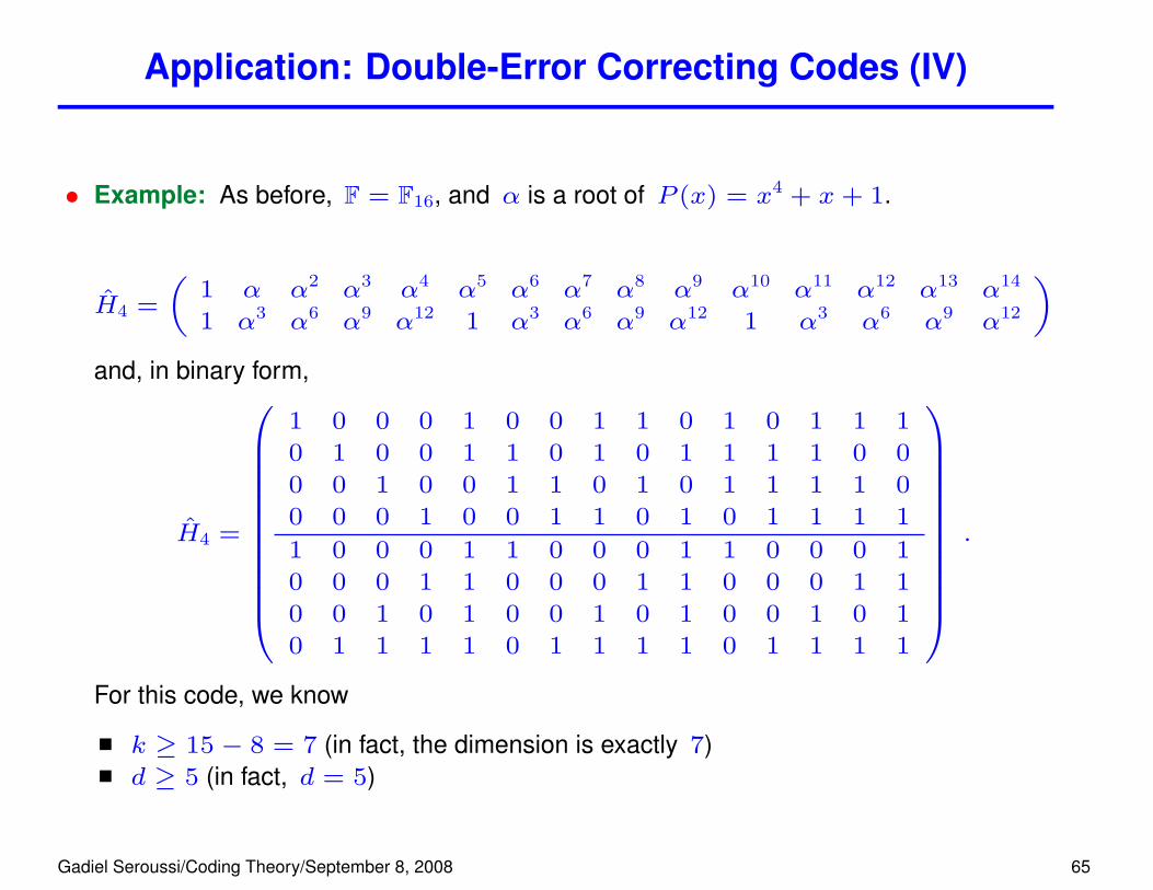
Application: Double-Error Correcting Codes (IV)
• Example: As before, F = F16, and α is a root of P (x) = x4 + x+ 1.
H4 =
„1 α α2 α3 α4 α5 α6 α7 α8 α9 α10 α11 α12 α13 α14
1 α3 α6 α9 α12 1 α3 α6 α9 α12 1 α3 α6 α9 α12
«and, in binary form,
H4 =
0BBBBBBBBBBB@
1 0 0 0 1 0 0 1 1 0 1 0 1 1 1
0 1 0 0 1 1 0 1 0 1 1 1 1 0 0
0 0 1 0 0 1 1 0 1 0 1 1 1 1 0
0 0 0 1 0 0 1 1 0 1 0 1 1 1 1
1 0 0 0 1 1 0 0 0 1 1 0 0 0 1
0 0 0 1 1 0 0 0 1 1 0 0 0 1 1
0 0 1 0 1 0 0 1 0 1 0 0 1 0 1
0 1 1 1 1 0 1 1 1 1 0 1 1 1 1
1CCCCCCCCCCCA.
For this code, we know
k ≥ 15− 8 = 7 (in fact, the dimension is exactly 7)d ≥ 5 (in fact, d = 5)
Gadiel Seroussi/Coding Theory/September 8, 2008 65

Variations on the Double-error Correcting Code
• Add an overall parity bit
H4 =
0@ 1 α α2 α3 α4 α5 α6 α7 α8 α9 α10 α11 α12 α13 α14 0
1 α3 α6 α9 α12 1 α3 α6 α9 α12 1 α3 α6 α9 α12 0
1 1 1 1 1 1 1 1 1 1 1 1 1 1 1 1
1AFor this code, we know
n = 16
k = 7 (same number of words)d = 6
corrects 2 errors, detects 3
• Expurgate words of odd weight
H4 =
0@ 1 α α2 α3 α4 α5 α6 α7 α8 α9 α10 α11 α12 α13 α14
1 α3 α6 α9 α12 1 α3 α6 α9 α12 1 α3 α6 α9 α12
1 1 1 1 1 1 1 1 1 1 1 1 1 1 1
1A
n = 15, k = 6, d = 6: corrects 2 errors, detects 3
Gadiel Seroussi/Coding Theory/September 8, 2008 66

5. Reed-Solomon Codes
Gadiel Seroussi/Coding Theory/September 8, 2008 67

Generalized Reed-Solomon Codes
• Let α1, α2, . . . , αn, n < q, be distinct nonzero elements of Fq, and letv1, v2, . . . , vn be nonzero elements of Fq (not necessarily distinct). Ageneralized Reed-Solomon (GRS) code is a linear [n, k, d] code CGRS
with PCM
HGRS =
0BBBBB@1 1 . . . 1
α1 α2 . . . αnα2
1 α22 . . . α2
n... ... ... ...αn−k−1
1 αn−k−12 . . . αn−k−1
n
1CCCCCA0BBB@
v1
v2 00 . . .
vn
1CCCA .
αj: code locators (distinct), vj:column multipliers ( 6= 0)
Reminder. CGRS is an MDS code, namely, d = n− k + 1.
Theorem. The dual of a GRS code is a GRS code.
Proof. Show that GGRS can have the same form as HGRS, with k rows, the samelocators, and a different choice of multipliers {v′i}. �
Gadiel Seroussi/Coding Theory/September 8, 2008 68

Distinguished Classes of GRS Codes
• Primitive GRS codes: n = q−1 and {α1, α2, . . . , αn} = F ∗; usually αi = αi−1 fora primitive α ∈ F.
• Normalized GRS codes: vj = 1 for all 1 ≤ j ≤ n.
• Narrow-sense GRS codes: vj = αj for all 1 ≤ j ≤ n.
• Allowing one αi = 0 (column [1 0 . . . 0]T , not in narrow sense GRS):(singly) extended GRS code ⇒ n ≤ q
• Allowing one αi =∞ (column [0 . . . 0 1]T , not in narrow sense GRS):(doubly) extended GRS code ⇒ n ≤ q + 1
Example: Let v1, v2, . . . , vn be the column multipliers of a primitive GRS code. Weverify that the dual GRS code has column multipliers αj/vj. Let α be a primitive elementof F. For v′j = αj/vj, a typical entry in the postulated G·HT is
Gi·HTh =
nX`=1
v`v′`α
i+h` =
nX`=1
αi+h+1` =
nX`=1
α(`−1)(i+h+1)
=αn(i+h+1) − 1
αi+h+1 − 1= 0
with 0≤i≤k−1, 0≤h≤n−k−1 and, thus, 0≤i+h+1≤n−1 (recall that O(α)=n).
⇒ (normalized primitive GRS)⊥ = (narrow-sense primitive GRS).
Gadiel Seroussi/Coding Theory/September 8, 2008 69
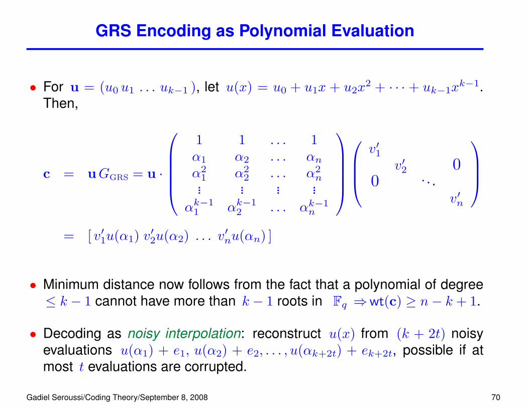
GRS Encoding as Polynomial Evaluation
• For u = (u0 u1 . . . uk−1 ), let u(x) = u0 + u1x + u2x2 + · · · + uk−1x
k−1.Then,
c = uGGRS = u ·
1 1 . . . 1α1 α2 . . . αnα2
1 α22 . . . α2
n... ... ... ...αk−1
1 αk−12 . . . αk−1
n
v′1v′2 0
0 . . .v′n
= [ v′1u(α1) v′2u(α2) . . . v′nu(αn) ]
• Minimum distance now follows from the fact that a polynomial of degree≤ k − 1 cannot have more than k − 1 roots in Fq ⇒wt(c) ≥ n− k + 1.
• Decoding as noisy interpolation: reconstruct u(x) from (k + 2t) noisyevaluations u(α1) + e1, u(α2) + e2, . . . , u(αk+2t) + ek+2t, possible if atmost t evaluations are corrupted.
Gadiel Seroussi/Coding Theory/September 8, 2008 70

Conventional Reed-Solomon Codes
• Conventional Reed-Solomon (RS) code: GRS code with n|(q−1), α ∈ F∗with O(α) = n,
αj = αj−1 , 1 ≤ j ≤ n,
vj = αb(j−1) , 1 ≤ j ≤ n .
• Canonical PCM of a RS code is given by
HRS =
1 αb . . . α(n−1)b
1 αb+1 . . . α(n−1)(b+1)
... ... ... ...1 αb+d−2 . . . α(n−1)(b+d−2)
(# rows = d−1 = n−k)
• c ∈ CRS ⇐⇒ HRScT = 0 ⇐⇒ c(α`) = 0, ` = b, b+1, . . . , b+d−2.
• αb, αb+1, . . . , αb+d−2: roots of CRS
• g(x) = (x− αb)(x− αb+1) · · · (x− αb+d−2) : generator polynomial of CRS
Gadiel Seroussi/Coding Theory/September 8, 2008 71
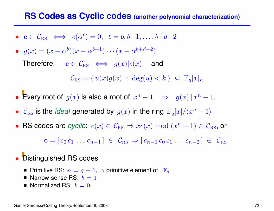
RS Codes as Cyclic codes (another polynomial characterization)
• c ∈ CRS ⇐⇒ c(α`) = 0, ` = b, b+1, . . . , b+d−2
• g(x) = (x− αb)(x− αb+1) · · · (x− αb+d−2)
Therefore, c ∈ CRS ⇐⇒ g(x)|c(x) and
CRS = {u(x)g(x) : deg(u) < k } ⊆ Fq[x]n
• Every root of g(x) is also a root of xn − 1 ⇒ g(x) |xn − 1.
• CRS is the ideal generated by g(x) in the ring Fq[x]/〈xn − 1〉
• RS codes are cyclic: c(x) ∈ CRS ⇒ xc(x) mod (xn − 1) ∈ CRS, or
c = [ c0 c1 . . . cn−1 ] ∈ CRS ⇒ [ cn−1 c0 c1 . . . cn−2 ] ∈ CRS
• Distinguished RS codes
Primitive RS: n = q − 1, α primitive element of FqNarrow-sense RS: b = 1
Normalized RS: b = 0
Gadiel Seroussi/Coding Theory/September 8, 2008 72

Encoding RS codes
• We can encode GRS codes as any linear code: u 7→ uGGRS
• In the polynomial interpretation of RS codes: u(x) 7→ u(x)g(x),corresponding to a non-systematic generator matrix
G =
g0 g1 . . . gn−k
g0 g1 . . . gn−k 00 . . . . . . · · · . . .
g0 g1 . . . gn−k
(gn−k = 1)
Gadiel Seroussi/Coding Theory/September 8, 2008 73

Non-systematic Encoding Circuit
u0u1 . . . uk−1 →t - - - -
? ? ?
· · ·
? ?
&%'$gr &%
'$gr−1 &%
'$gr−2 · · ·&%
'$g1 &%
'$g0
r = n− k?
HHHH
HHHHHH
HHHHHj
@@@@@@R
���
���
����
������
������
&%'$+
-tc0c1 . . . cn−1 →
- -
1 clock cycledelay unit
"!# gi?
?
multiplyby gi
"!#
"!# +
@@R
��
?
add
Gadiel Seroussi/Coding Theory/September 8, 2008 74
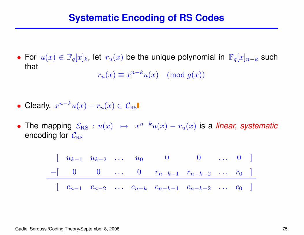
Systematic Encoding of RS Codes
• For u(x) ∈ Fq[x]k, let ru(x) be the unique polynomial in Fq[x]n−k suchthat
ru(x) ≡ xn−ku(x) (mod g(x))
• Clearly, xn−ku(x)− ru(x) ∈ CRS
• The mapping ERS : u(x) 7→ xn−ku(x) − ru(x) is a linear, systematicencoding for CRS
[ uk−1 uk−2 . . . u0 0 0 . . . 0 ]
−[ 0 0 . . . 0 rn−k−1 rn−k−2 . . . r0 ]
[ cn−1 cn−2 . . . cn−k cn−k−1 cn−k−2 . . . c0 ]
Gadiel Seroussi/Coding Theory/September 8, 2008 75

Systematic Encoding Circuit
&%'$+ &%
'$+ · · · &%
'$+ &%
'$+
&%'$g0 &%
'$g1 &%
'$g2 · · · &%
'$gn−k−1 &%
'$−1
- - - - - - - -
? ? ? ?
? ? ?
6
6
· · · tA @@@@I
�
t B
tu0u1 . . . uk−1 →
-tB�
���
z
6t A
-tc0c1 . . . cn−1 →
• Switchesat A for k cyclesat B for n− k cycles
• Register contents: R0(x) = 0;
R`(x) = xR`−1(x) + xruk−`
= xn−kX
i=1
uk−ix`−i
mod g(x)
` = 1, 2, . . . , k .
Gadiel Seroussi/Coding Theory/September 8, 2008 76

6. Decoding GeneralizedReed-Solomon Codes
Gadiel Seroussi/Coding Theory/September 8, 2008 77

Decoding Generalized Reed-Solomon Codes
• We consider CGRS over Fq with PCM
HGRS =
1 1 . . . 1α1 α2 . . . αnα2
1 α22 . . . α2
n... ... ... ...αd−2
1 αd−22 . . . αd−2
n
v1
v2 00 . . .
vn
with α1, α2, . . . , αn ∈ F∗q distinct, and v1, v2, . . . , vn ∈ F∗q
• Codeword c transmitted, word y received, with error vector
e = (e1 e2 . . . en) = y − c
• J = {κ : eκ 6= 0} set of error locations
• We describe and algorithm that correctly decodes y to c, under theassumption |J | ≤ 1
2(d−1).
Gadiel Seroussi/Coding Theory/September 8, 2008 78

Syndrome Computation
• First step of the decoding algorithm
S =
S0
S1...
Sd−2
= HGRSyT = HGRSeT
S` =n∑j=1
yjvjα`j =
n∑j=1
ejvjα`j =
∑j∈J
ejvjα`j , ` = 0, 1, . . . , d−2
Example: For RS codes, we have αj = αj−1 and vj = αb(j−1), so
S` =
nXj=1
yjα(j−1)(b+`)
= y(αb+`
) , ` = 0, 1, . . . , d−2 .
• Syndrome polynomial :
S(x) =d−2∑`=0
S`x` =
d−2∑`=0
x`∑j∈J
ejvjα`j =
∑j∈J
ejvj
d−2∑`=0
(αjx)` .
Gadiel Seroussi/Coding Theory/September 8, 2008 79

A Congruence for the Syndrome Polynomial
S(x) =∑j∈J
ejvj
d−2∑`=0
(αjx)` .
• We haved−2∑`=0
(αjx)` ≡ 11− αjx
(mod xd−1)
⇒ S(x) =∑j∈J
ejvj1− αjx
(mod xd−1)(∑
φ� = 0)
Gadiel Seroussi/Coding Theory/September 8, 2008 80
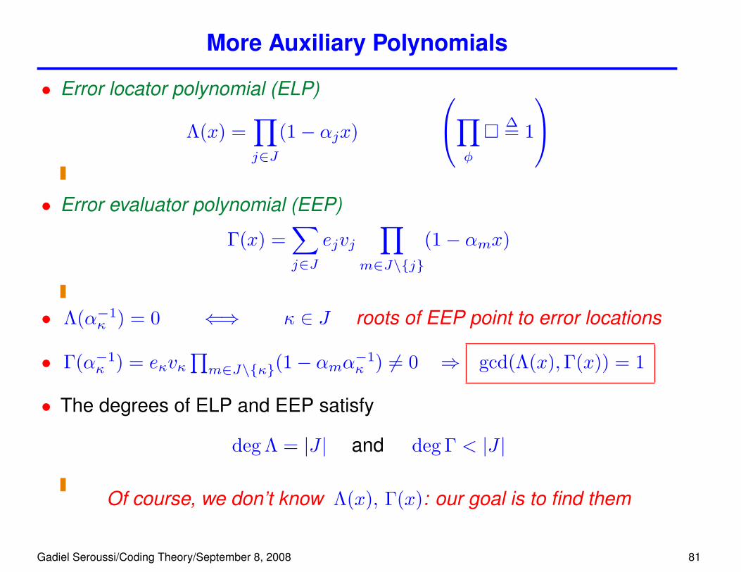
More Auxiliary Polynomials
• Error locator polynomial (ELP)
Λ(x) =∏j∈J
(1− αjx)
∏φ
�∆= 1
• Error evaluator polynomial (EEP)
Γ(x) =∑j∈J
ejvj∏
m∈J\{j}
(1− αmx)
• Λ(α−1κ ) = 0 ⇐⇒ κ ∈ J roots of EEP point to error locations
• Γ(α−1κ ) = eκvκ
∏m∈J\{κ}(1− αmα−1
κ ) 6= 0 ⇒ gcd(Λ(x),Γ(x)) = 1
• The degrees of ELP and EEP satisfy
deg Λ = |J | and deg Γ < |J |
Of course, we don’t know Λ(x), Γ(x): our goal is to find them
Gadiel Seroussi/Coding Theory/September 8, 2008 81
Key Equation of GRS Decoding
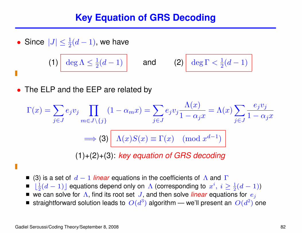
• Since |J | ≤ 12(d− 1), we have
(1) deg Λ ≤ 12(d− 1) and (2) deg Γ < 1
2(d− 1)
• The ELP and the EEP are related by
Γ(x) =∑j∈J
ejvj∏
m∈J\{j}
(1− αmx) =∑j∈J
ejvjΛ(x)
1− αjx= Λ(x)
∑j∈J
ejvj1− αjx
=⇒ (3) Λ(x)S(x) ≡ Γ(x) (mod xd−1)
(1)+(2)+(3): key equation of GRS decoding
(3) is a set of d− 1 linear equations in the coefficients of Λ and Γ
b12(d− 1)c equations depend only on Λ (corresponding to xi, i ≥ 1
2(d− 1))we can solve for Λ, find its root set J , and then solve linear equations for ejstraightforward solution leads to O(d3) algorithm — we’ll present an O(d2) one
Gadiel Seroussi/Coding Theory/September 8, 2008 82
The Extended Euclidean Algorithm
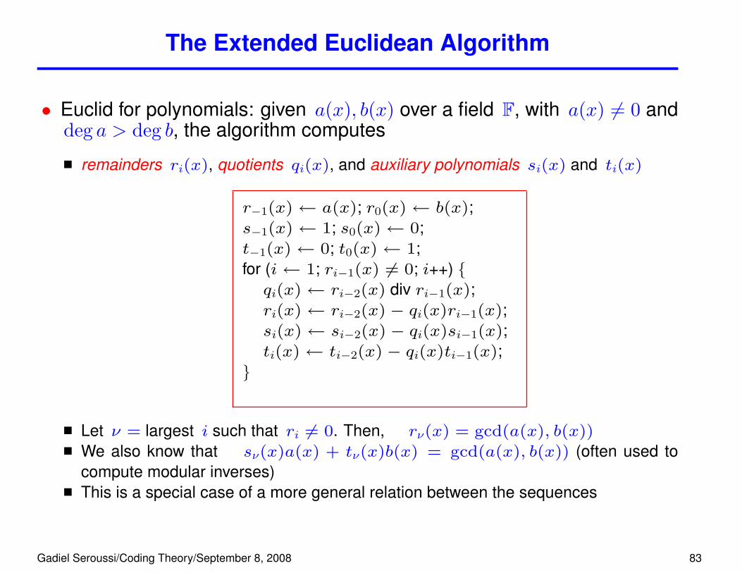
• Euclid for polynomials: given a(x), b(x) over a field F, with a(x) 6= 0 anddeg a > deg b, the algorithm computes
remainders ri(x), quotients qi(x), and auxiliary polynomials si(x) and ti(x)
r−1(x)← a(x); r0(x)← b(x);s−1(x)← 1; s0(x)← 0;t−1(x)← 0; t0(x)← 1;for (i← 1; ri−1(x) 6= 0; i++) {qi(x)← ri−2(x) div ri−1(x);ri(x)← ri−2(x)− qi(x)ri−1(x);si(x)← si−2(x)− qi(x)si−1(x);ti(x)← ti−2(x)− qi(x)ti−1(x);
}
Let ν = largest i such that ri 6= 0. Then, rν(x) = gcd(a(x), b(x))
We also know that sν(x)a(x) + tν(x)b(x) = gcd(a(x), b(x)) (often used tocompute modular inverses)This is a special case of a more general relation between the sequences
Gadiel Seroussi/Coding Theory/September 8, 2008 83
Properties of the Euclidean Algorithm Sequences
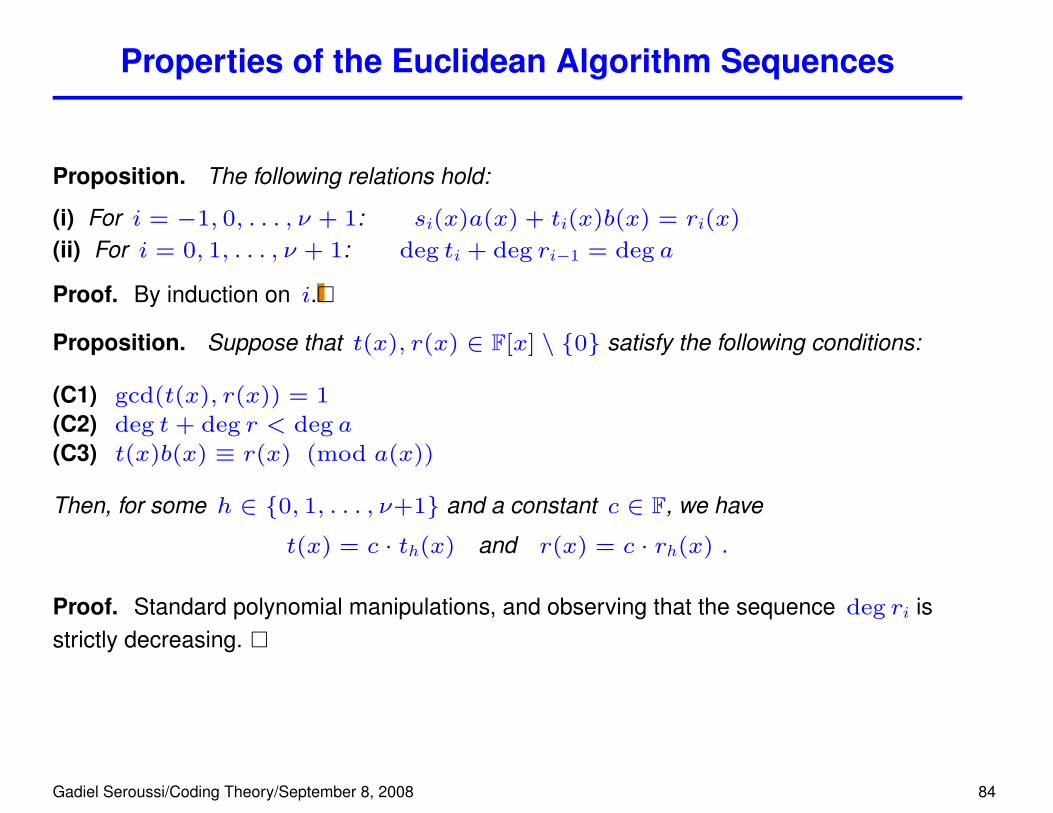
Proposition. The following relations hold:
(i) For i = −1, 0, . . . , ν + 1: si(x)a(x) + ti(x)b(x) = ri(x)
(ii) For i = 0, 1, . . . , ν + 1: deg ti + deg ri−1 = deg a
Proof. By induction on i.�
Proposition. Suppose that t(x), r(x) ∈ F[x] \ {0} satisfy the following conditions:
(C1) gcd(t(x), r(x)) = 1
(C2) deg t+ deg r < deg a
(C3) t(x)b(x) ≡ r(x) (mod a(x))
Then, for some h ∈ {0, 1, . . . , ν+1} and a constant c ∈ F, we have
t(x) = c · th(x) and r(x) = c · rh(x) .
Proof. Standard polynomial manipulations, and observing that the sequence deg ri isstrictly decreasing. �
Gadiel Seroussi/Coding Theory/September 8, 2008 84
Solving the Key Equation
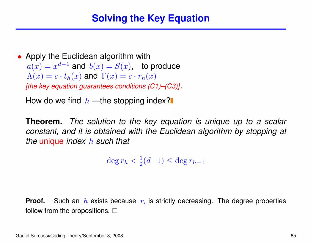
• Apply the Euclidean algorithm witha(x) = xd−1 and b(x) = S(x), to produceΛ(x) = c · th(x) and Γ(x) = c · rh(x)[the key equation guarantees conditions (C1)–(C3)].
How do we find h —the stopping index?
Theorem. The solution to the key equation is unique up to a scalarconstant, and it is obtained with the Euclidean algorithm by stopping atthe unique index h such that
deg rh < 12(d−1) ≤ deg rh−1
Proof. Such an h exists because ri is strictly decreasing. The degree propertiesfollow from the propositions. �
Gadiel Seroussi/Coding Theory/September 8, 2008 85
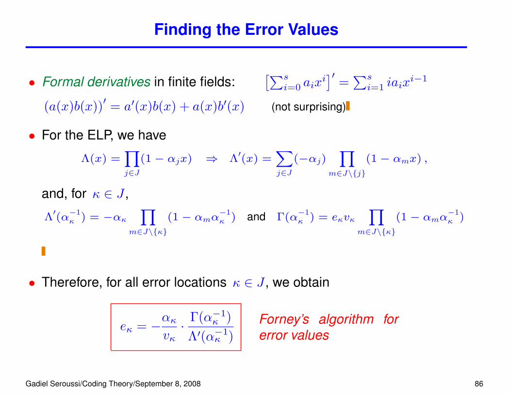
Finding the Error Values
• Formal derivatives in finite fields:[∑s
i=0 aixi]′ = ∑s
i=1 iaixi−1
(a(x)b(x))′ = a′(x)b(x) + a(x)b′(x) (not surprising)
• For the ELP, we have
Λ(x) =Yj∈J
(1− αjx) ⇒ Λ′(x) =
Xj∈J
(−αj)Y
m∈J\{j}
(1− αmx) ,
and, for κ ∈ J ,
Λ′(α−1κ ) = −ακ
Ym∈J\{κ}
(1− αmα−1κ ) and Γ(α
−1κ ) = eκvκ
Ym∈J\{κ}
(1− αmα−1κ )
• Therefore, for all error locations κ ∈ J , we obtain
eκ = −ακvκ· Γ(α−1
κ )Λ′(α−1
κ )Forney’s algorithm forerror values
Gadiel Seroussi/Coding Theory/September 8, 2008 86
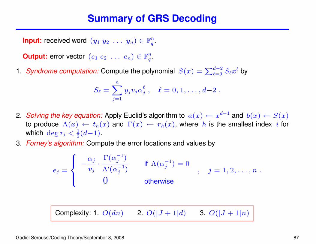
Summary of GRS Decoding
Input: received word (y1 y2 . . . yn) ∈ Fnq .
Output: error vector (e1 e2 . . . en) ∈ Fnq .
1. Syndrome computation: Compute the polynomial S(x) =Pd−2
`=0 S`x` by
S` =
nXj=1
yjvjα`j , ` = 0, 1, . . . , d−2 .
2. Solving the key equation: Apply Euclid’s algorithm to a(x)← xd−1 and b(x)← S(x)
to produce Λ(x) ← th(x) and Γ(x) ← rh(x), where h is the smallest index i forwhich deg ri <
12(d−1).
3. Forney’s algorithm: Compute the error locations and values by
ej =
8>><>>:−αj
vj·
Γ(α−1j )
Λ′(α−1j )
if Λ(α−1j ) = 0
0 otherwise
, j = 1, 2, . . . , n .
Complexity: 1. O(dn) 2. O(|J + 1|d) 3. O(|J + 1|n)
Gadiel Seroussi/Coding Theory/September 8, 2008 87
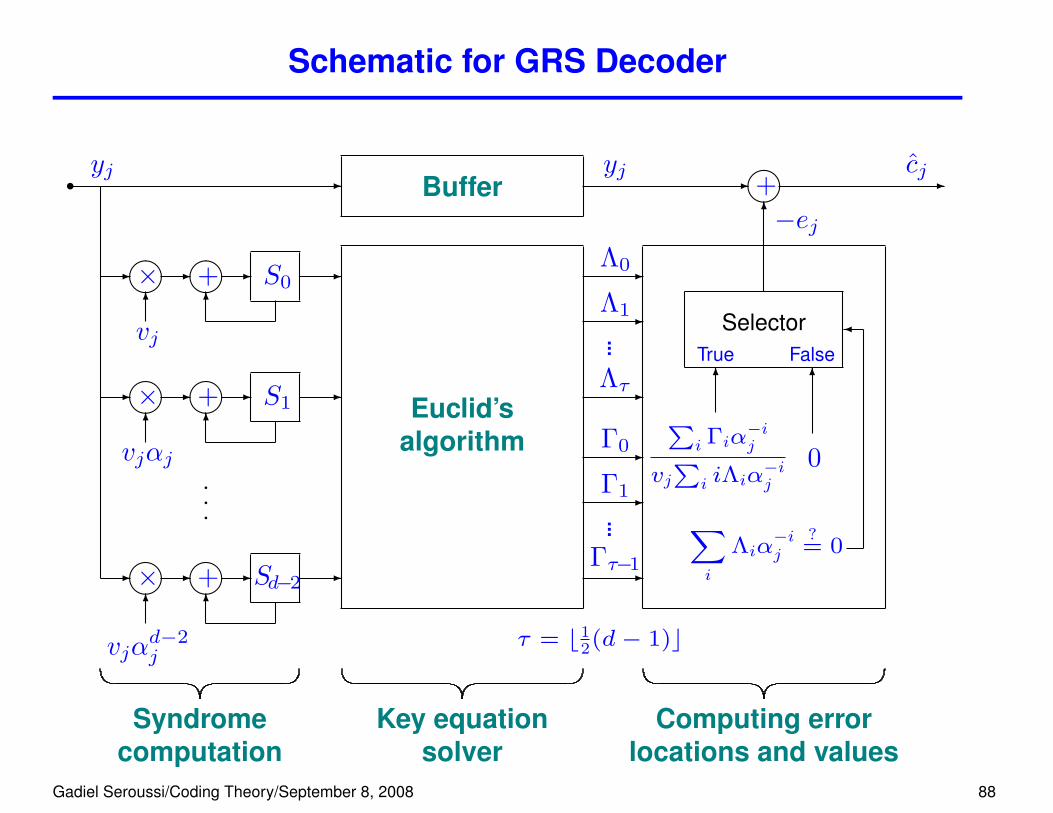
Schematic for GRS Decoder
t -yj
Bufferyj
-����+ -
cj
����× ����+ S0
- - - -
66
vj
����× ����+ S1
- - - -
66
vjαj qqq
����× ����+ Sd−2
- - - -
66
vjαd−2j
Euclid’salgorithm
-Λ0
-Λ1
...-
Λτ
-Γ0
-Γ1
...-
Γτ−1
SelectorTrue6
Pi Γiα
−ij
vjP
i iΛiα−ij
False6
0
�
Xi
Λiα−ij
?= 0
6−ej
Syndromecomputation
Key equationsolver
Computing errorlocations and values
τ = b12(d− 1)c
Gadiel Seroussi/Coding Theory/September 8, 2008 88

Finding Roots of the ELP (RS Codes)
Chien search for RS codes (αj = αj−1, 1 ≤ j ≤ n)
����× Λτ ��
��+
6
- - -
6
α−τ
����× Λ1 ��
��+
6
- - -
6
α−1
Λ0-����+
6
...6
Λ(α−j+1)
At clock cycle # j, thecell labeled Λi contains
Λiα−i(j−1), 0 ≤ i ≤ τ, 1 ≤ j ≤ n
Gadiel Seroussi/Coding Theory/September 8, 2008 89

RS Decoding Example
Example
Gadiel Seroussi/Coding Theory/September 8, 2008 90
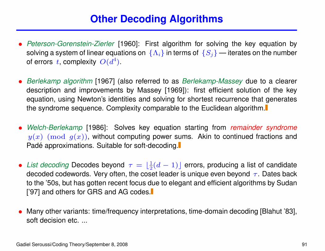
Other Decoding Algorithms
• Peterson-Gorenstein-Zierler [1960]: First algorithm for solving the key equation bysolving a system of linear equations on {Λi} in terms of {Sj}— iterates on the numberof errors t, complexity O(d4).
• Berlekamp algorithm [1967] (also referred to as Berlekamp-Massey due to a clearerdescription and improvements by Massey [1969]): first efficient solution of the keyequation, using Newton’s identities and solving for shortest recurrence that generatesthe syndrome sequence. Complexity comparable to the Euclidean algorithm.
• Welch-Berlekamp [1986]: Solves key equation starting from remainder syndromey(x) (mod g(x)), without computing power sums. Akin to continued fractions andPade approximations. Suitable for soft-decoding.
• List decoding Decodes beyond τ = b12(d − 1)c errors, producing a list of candidate
decoded codewords. Very often, the coset leader is unique even beyond τ . Dates backto the ’50s, but has gotten recent focus due to elegant and efficient algorithms by Sudan[’97] and others for GRS and AG codes.
• Many other variants: time/frequency interpretations, time-domain decoding [Blahut ’83],soft decision etc. ...
Gadiel Seroussi/Coding Theory/September 8, 2008 91

7. Codes Related to GRS Codes
Gadiel Seroussi/Coding Theory/September 8, 2008 92
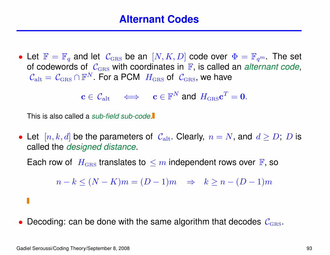
Alternant Codes
• Let F = Fq and let CGRS be an [N,K,D] code over Φ = Fqm. The setof codewords of CGRS with coordinates in F, is called an alternant code,Calt = CGRS ∩ FN . For a PCM HGRS of CGRS, we have
c ∈ Calt ⇐⇒ c ∈ FN and HGRScT = 0.
This is also called a sub-field sub-code.
• Let [n, k, d] be the parameters of Calt. Clearly, n = N , and d ≥ D; D iscalled the designed distance.
Each row of HGRS translates to ≤ m independent rows over F, so
n− k ≤ (N −K)m = (D − 1)m ⇒ k ≥ n− (D − 1)m
• Decoding: can be done with the same algorithm that decodes CGRS.
Gadiel Seroussi/Coding Theory/September 8, 2008 93
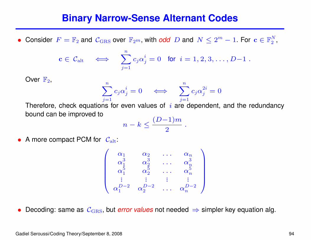
Binary Narrow-Sense Alternant Codes
• Consider F = F2 and CGRS over F2m, with odd D and N ≤ 2m − 1. For c ∈ FN2 ,
c ∈ Calt ⇐⇒nXj=1
cjαij = 0 for i = 1, 2, 3, . . . , D−1 .
Over F2,nXj=1
cjαij = 0 ⇐⇒
nXj=1
cjα2ij = 0
Therefore, check equations for even values of i are dependent, and the redundancybound can be improved to
n− k ≤(D−1)m
2.
• A more compact PCM for Calt:0BBBBB@α1 α2 . . . αnα3
1 α32 . . . α3
n
α51 α5
2 . . . α5n... ... ... ...
αD−21 αD−2
2 . . . αD−2n
1CCCCCA• Decoding: same as CGRS, but error values not needed ⇒ simpler key equation alg.
Gadiel Seroussi/Coding Theory/September 8, 2008 94

BCH Codes
• Bose-Chaudhuri-Hocquenghem (BCH) codes are alternant codes that correspond toconventional RS codes, i.e., for CRS : [N,K,D] over Fqm, CBCH = FNq ∩ CRS.
• N must divide qm − 1 ⇒ gcd(N, q) = 1. Conversely, if gcd(N, q) = 1, then q
belongs to the multiplicative group of the integers modulo N . So, given a code lengthn = N , the smallest possible value of m is the order of q in the multiplicative groupmodulo N .
Summary of BCH code definition
• Code of length n ≥ 1 over Fq such that gcd(n, q) = 1
• m ≥ 1: [smallest] positive integer s.t. n|qm − 1
• α ∈ Fqm: element of multiplicative order n• D > 0, b: design parameters
CBCH =nc(x) ∈ (Fq)n[x] : c(α
`) = 0, ` = b, b+ 1, . . . , b+D − 2
o
Gadiel Seroussi/Coding Theory/September 8, 2008 95

BCH Code Example
Example: We design a BCH code of length n = 85 over F2 that can correct 3 errors.
• m = smallest positive integer s.t. 85|2m−1 ⇒m = 8.• b = 1 ⇒ narrow-sense• D = 7 ⇒ 3-error correcting• n− k ≤ (D−1)m/2 = 24
• resulting CBCH is [85,≥61,≥7] over F2
• Let γ be a primitive element of Φ = F28, α = γ3, so that O(α) = 85.• a 24× 85 binary PCM of the code can be obtained by representing the entries in HΦ
below as column vectors in F82.
HΦ =
0@ 1 α α2 . . . αj . . . α83 α84
1 α3 α6 . . . α3j . . . α79 α82
1 α5 α10 . . . α5j . . . α75 α80
1A• Let γ be a root of p(x) = x8 + x6 + x5 + x + 1 (primitive polynomial). Represent
F28 = F2(γ) ≡ F2[x]/〈p(x)〉. Then,
α = γ3 ↔ [00010000]T
α3 = γ9 = γ + γ2 + γ6 + γ7 ↔ [01100011]T
α5 = γ15 = γ3 + γ6 + γ7 ↔ [00010011]T
The second column in HF2will be [00010000 01100011 00010011]T
Gadiel Seroussi/Coding Theory/September 8, 2008 96
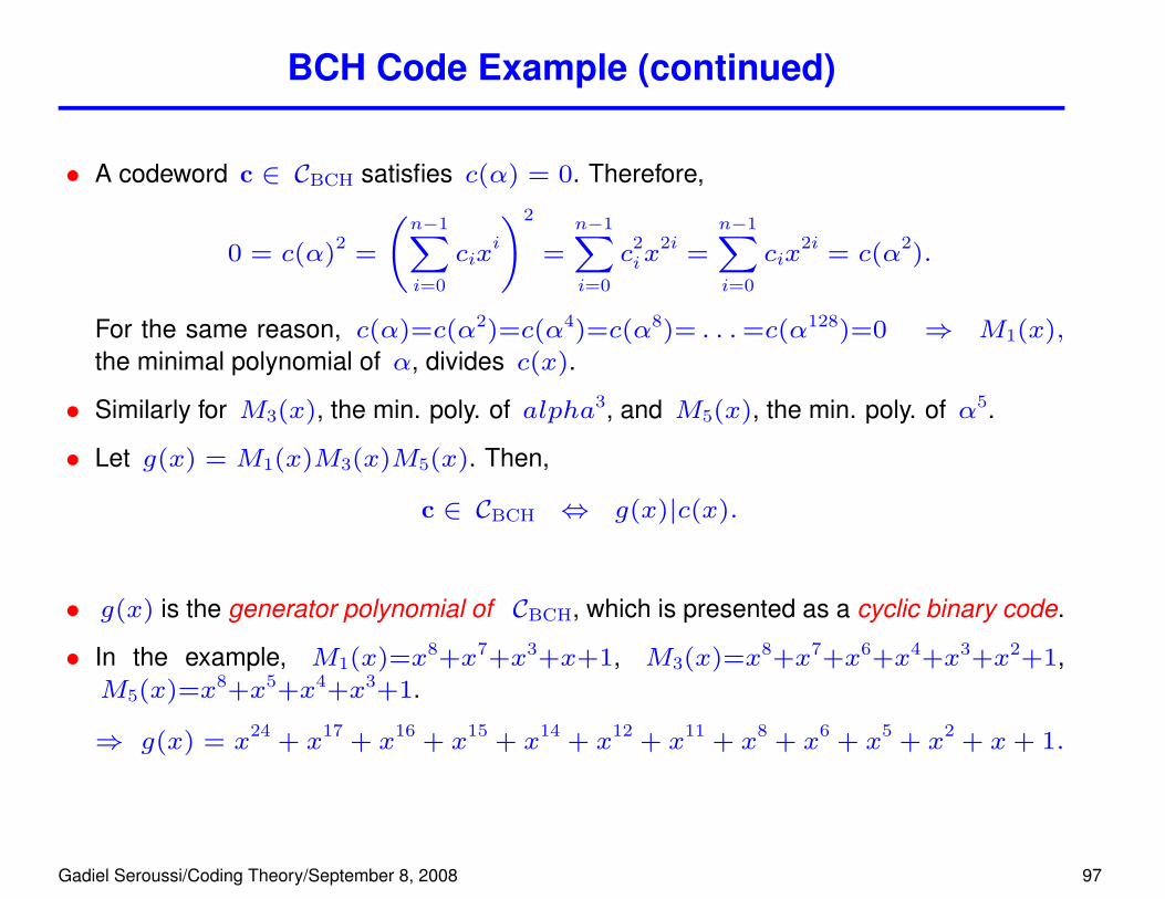
BCH Code Example (continued)
• A codeword c ∈ CBCH satisfies c(α) = 0. Therefore,
0 = c(α)2
=
n−1Xi=0
cixi
!2
=
n−1Xi=0
c2ix
2i=
n−1Xi=0
cix2i
= c(α2).
For the same reason, c(α)=c(α2)=c(α4)=c(α8)= . . .=c(α128)=0 ⇒ M1(x),
the minimal polynomial of α, divides c(x).
• Similarly for M3(x), the min. poly. of alpha3, and M5(x), the min. poly. of α5.
• Let g(x) = M1(x)M3(x)M5(x). Then,
c ∈ CBCH ⇔ g(x)|c(x).
• g(x) is the generator polynomial of CBCH, which is presented as a cyclic binary code.
• In the example, M1(x)=x8+x7+x3+x+1, M3(x)=x8+x7+x6+x4+x3+x2+1,M5(x)=x8+x5+x4+x3+1.
⇒ g(x) = x24
+ x17
+ x16
+ x15
+ x14
+ x12
+ x11
+ x8
+ x6
+ x5
+ x2
+ x+ 1.
Gadiel Seroussi/Coding Theory/September 8, 2008 97

BCH Code Example (continued)
• As with RS codes, we have the polynomial (cyclic) interpretation of BCH codes:u(x) 7→ c(x)=u(x)g(x), with u(x) ∈ F2[x] (a binary polynomial of degree < k),corresponding to a non-systematic binary generator matrix
G =
0BBB@g0 g1 . . . gn−k
g0 g1 . . . gn−k 00 . . . . . . · · · . . .
g0 g1 . . . gn−k
1CCCA (gn−k = 1)
• In the example, this representation also implies that kBCH = 85 − 24 = 61, the rankof G.
• Codes with dimension better than the bound are obtained when some of the minimalpolynomials Mi are of degree less than m.
• such a code would be obtained, for example, if we changed the parameter b so thatα17 were one of the roots. In this case (no longer a narrow sense code), we have
O(α17
) = 5 ⇒ M17(x) = x4+x
3+x
2+x+1,
i.e.,α
17 ∈ F16 ⊂ F256.
Gadiel Seroussi/Coding Theory/September 8, 2008 98

MDS Codes and the MDS Conjecture
• MDS codes satisfy the Singleton bound with equality: d = n− k + 1
• GRS codes are MDS
there exist GRS codes with parameters [n, k, n− k+ 1], 1 ≤ k ≤ n ≤ q + 1, forall finite fields Fqrecall that lengths q, q + 1 can be obtained using column locators 0 and ∞
when q = 2m and k = 3, the matrix0@ 1 1 . . . 1 1 0 0
α1 α2 . . . αq−1 0 1 0
α21 α2
2 . . . α2q−1 0 0 1
1A generates a [q + 2, 3, q] linear MDStriply-extended GRS code;its dual is a [q + 2, q − 1, 4] MDS code
the [n, n, 1] full space, [n, 1, n] repetition code, and the [n, n − 1, 2] parity codeare MDS, for any lengthn and field Fqno other non-trivial MDS codes of length > q + 1 are known. Let
Lq(k) = max{n : ∃ [n, k, n− k + 1] MDS code over Fq }.
The MDS Conjecture. Lq(k) = q + 1, except for the cases listed above.
Gadiel Seroussi/Coding Theory/September 8, 2008 99
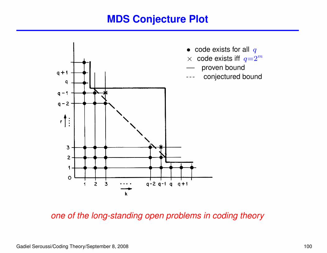
MDS Conjecture Plot
• code exists for all q× code exists iff q=2m
proven boundconjectured bound
one of the long-standing open problems in coding theory
Gadiel Seroussi/Coding Theory/September 8, 2008 100
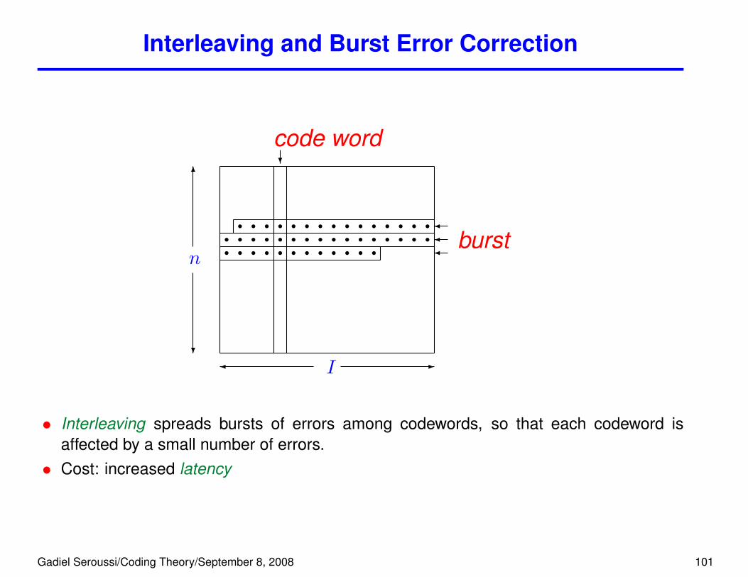
Interleaving and Burst Error Correction
?
code word
?
6
n
�
�
�burst
� -I
s s s s s s s s s s s s s s ss s s s s s s s s s s s s s s ss s s s s s s s s s s s
• Interleaving spreads bursts of errors among codewords, so that each codeword isaffected by a small number of errors.
• Cost: increased latency
Gadiel Seroussi/Coding Theory/September 8, 2008 101
Concatenated Codes
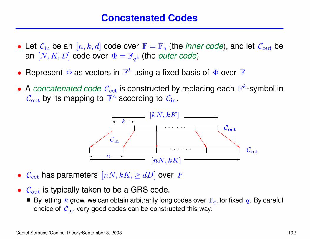
• Let Cin be an [n, k, d] code over F = Fq (the inner code), and let Cout bean [N,K,D] code over Φ = Fqk (the outer code)
• Represent Φ as vectors in Fk using a fixed basis of Φ over F
• A concatenated code Ccct is constructed by replacing each Fk-symbol inCout by its mapping to Fn according to Cin.
· · · · · ·
· · · · · ·�
��
���=
� ?
JJJJJ
ZZZZZZ~
� k -
� -n
Cin
Ccct
Cout
� [kN, kK] -
� -[nN, kK]
• Ccct has parameters [nN, kK,≥ dD] over F
• Cout is typically taken to be a GRS code.By letting k grow, we can obtain arbitrarily long codes over Fq, for fixed q. By carefulchoice of Cin, very good codes can be constructed this way.
Gadiel Seroussi/Coding Theory/September 8, 2008 102