introduction to coding theory - tu berlin · introduction to coding theory 16. outline 1 code...
TRANSCRIPT
Introduction to Coding Theory
Sven PuchingerInstitute of Communications Engineering, Ulm University
COSIP Winter Retreat, 7.12.2016
Introduction to Coding Theory 1

Coding Theory
code node
E
Encoder Channel Decoder
Introduction to Coding Theory 2

Coding Theory
code
node
E
Encoder Channel Decoder
Introduction to Coding Theory 2

Coding Theory
code
node
E
Encoder Channel Decoder
Introduction to Coding Theory 2

Coding Theory
code node
E
Encoder Channel Decoder
Introduction to Coding Theory 2

Coding Theory
code node
E
Encoder Channel Decoder
Introduction to Coding Theory 2
Coding Theory
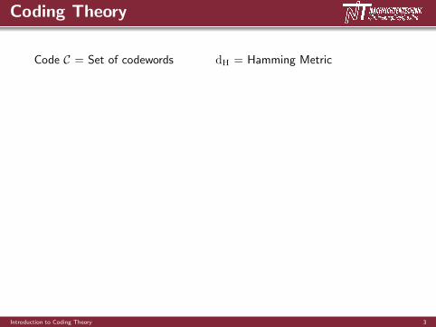
Code C = Set of codewords dH = Hamming Metric
C = {code, node, core}
dH(code,node) = 1, dH(code, core) = 1, dH(node, core) = 2
C = {simplifications, overgeneralized}
dH(simplifications, overgeneralized) = 13
Encoding (Rate R = kn )
k n
Information Codeword
Introduction to Coding Theory 3

Coding Theory
Code C = Set of codewords dH = Hamming Metric
C = {code, node, core}
dH(code,node) = 1, dH(code, core) = 1, dH(node, core) = 2
C = {simplifications, overgeneralized}
dH(simplifications, overgeneralized) = 13
Encoding (Rate R = kn )
k n
Information Codeword
Introduction to Coding Theory 3
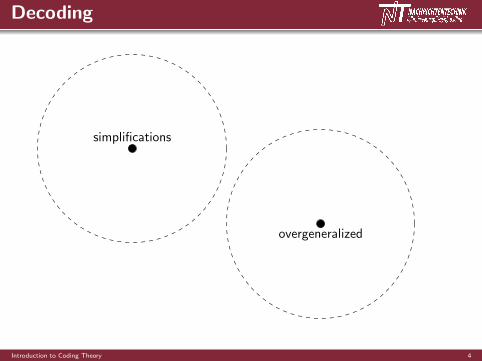
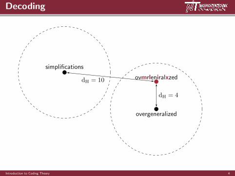
Decoding
simplifications
overgeneralized
ovmrleniralxzeddH = 10
dH = 4
Introduction to Coding Theory 4

Decoding
simplifications
overgeneralized
ovmrleniralxzed
dH = 10
dH = 4
Introduction to Coding Theory 4
Decoding
simplifications
overgeneralized
ovmrleniralxzeddH = 10
dH = 4
Introduction to Coding Theory 4

Coding Theory
Claude E. Shannon,A Mathematical Theory ofCommunication, 1948
If R < C, Perr → 0 (n→∞)
Richard Hamming,Error Detection and ErrorCorrection Codes, 1950
First Practical Codes
Introduction to Coding Theory 5

Coding Theory
Claude E. Shannon,A Mathematical Theory ofCommunication, 1948
If R < C, Perr → 0 (n→∞)
Richard Hamming,Error Detection and ErrorCorrection Codes, 1950
First Practical Codes
Introduction to Coding Theory 5

Jim Massey’s History of Channel Coding
Experts’ opinions
In the 50s and 60s
Coding is dead! All interesting problems are already solved.
In the 70s
Coding is dead as a doornail, except on the deep-space channel.
In the 80s
Coding is quite dead, except on wideband channels such as thedeep-space channel and narrowband channels such as the telephonechannel.
In the 90s
Coding is truly dead, except on single sender channels.
Introduction to Coding Theory 6
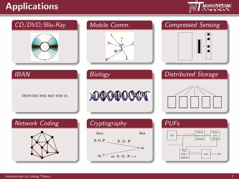
Applications
CD/DVD/Blu-Ray Mobile Comm. Compressed Sensing
· =
IBAN
DE78 0192 2932 3627 6328 10
Biology Distributed Storage
Network Coding Cryptography
Alice Bob
S,G,P
m
S ·G ·P
m m · S ·G ·P+ e
PUFs
PUF
r′ = c+ e+ e′
Helper
Data Ge-
neration
r = c+ e eHelper
Data
Storage
e
Key
Repro-
duction
r = c+ eHash Key
Introduction to Coding Theory 7

Applications
Experts’ opinion
Coding is surely dead, except on the deep-space channel, on narrowbandone-sender channels such as the telephone channel, on many senderchannels, storage, networks, ...
Introduction to Coding Theory 8

Outline
1 Code Constructions
2 Channels & Metrics
3 Decoding
4 Connection to Compressed Sensing
Introduction to Coding Theory 9

Outline
1 Code Constructions
2 Channels & Metrics
3 Decoding
4 Connection to Compressed Sensing
Introduction to Coding Theory 10

Code
K Field (usually finite, e.g. K = F2)
Code
C ⊂ Kn
Goal: Codewords c1, c2 ∈ C “far apart” w.r.t. a metric
d : Kn ×Kn → R≥0
Example: Hamming Metric
dH(x,y) = wtH(x− y), wtH(x) = |supp(x)|
Introduction to Coding Theory 11

Linear Block Codes
C(n, k, d) ⊆ Kn
Length n
K-subspace of dimension k
Minimum distance d
d = minc1,c2∈Cc1 6=c2
d(c1, c2) = minc∈C\{0}
wt(c)
Singleton Bound d ≤ n− k + 1
Introduction to Coding Theory 12

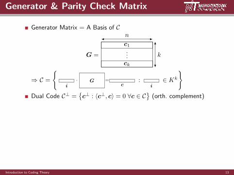
Generator & Parity Check Matrix
Generator Matrix = A Basis of C
G =
c1...ck
n
k
⇒ C =
{· =
i cG :
i∈ Kk
}Dual Code C⊥ =
{c⊥ : 〈c⊥, c〉 = 0 ∀c ∈ C
}(orth. complement)
Parity Check Matrix = A Basis of C⊥
H =
c⊥1...
c⊥n−k
n
n− k
⇒ C ={c ∈ Kn : HcT = 0
}
Introduction to Coding Theory 13

Generator & Parity Check Matrix
Generator Matrix = A Basis of C
G =
c1...ck
n
k
⇒ C =
{· =
i cG :
i∈ Kk
}
Dual Code C⊥ ={c⊥ : 〈c⊥, c〉 = 0 ∀c ∈ C
}(orth. complement)
Parity Check Matrix = A Basis of C⊥
H =
c⊥1...
c⊥n−k
n
n− k
⇒ C ={c ∈ Kn : HcT = 0
}
Introduction to Coding Theory 13
Generator & Parity Check Matrix
Generator Matrix = A Basis of C
G =
c1...ck
n
k
⇒ C =
{· =
i cG :
i∈ Kk
}Dual Code C⊥ =
{c⊥ : 〈c⊥, c〉 = 0 ∀c ∈ C
}(orth. complement)
Parity Check Matrix = A Basis of C⊥
H =
c⊥1...
c⊥n−k
n
n− k
⇒ C ={c ∈ Kn : HcT = 0
}
Introduction to Coding Theory 13

Generator & Parity Check Matrix
Generator Matrix = A Basis of C
G =
c1...ck
n
k
⇒ C =
{· =
i cG :
i∈ Kk
}Dual Code C⊥ =
{c⊥ : 〈c⊥, c〉 = 0 ∀c ∈ C
}(orth. complement)
Parity Check Matrix = A Basis of C⊥
H =
c⊥1...
c⊥n−k
n
n− k
⇒ C ={c ∈ Kn : HcT = 0
}
Introduction to Coding Theory 13

Generator & Parity Check Matrix
Generator Matrix = A Basis of C
G =
c1...ck
n
k
⇒ C =
{· =
i cG :
i∈ Kk
}Dual Code C⊥ =
{c⊥ : 〈c⊥, c〉 = 0 ∀c ∈ C
}(orth. complement)
Parity Check Matrix = A Basis of C⊥
H =
c⊥1...
c⊥n−k
n
n− k
⇒ C ={c ∈ Kn : HcT = 0
}Introduction to Coding Theory 13

Example 1: Repetition Code
K = F2
Code
C(n, 1, n) = {(00 . . . 0), (11 . . . 1)}
Generator Matrix
G =(1 1 . . . 1
)∈ F1×n
2
Parity Check Matrix
H =
1 1
1 1
. . ....
1 1
∈ Fn−1×n2
Introduction to Coding Theory 14

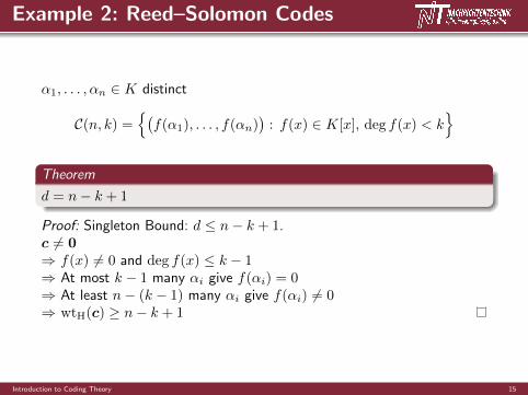
Example 2: Reed–Solomon Codes
α1, . . . , αn ∈ K distinct
C(n, k) ={(f(α1), . . . , f(αn)
): f(x) ∈ K[x], deg f(x) < k
}
Theorem
d = n− k + 1
Proof: Singleton Bound: d ≤ n− k + 1.c 6= 0⇒ f(x) 6= 0 and deg f(x) ≤ k − 1⇒ At most k − 1 many αi give f(αi) = 0⇒ At least n− (k − 1) many αi give f(αi) 6= 0⇒ wtH(c) ≥ n− k + 1
Introduction to Coding Theory 15

Example 2: Reed–Solomon Codes
α1, . . . , αn ∈ K distinct
C(n, k) ={(f(α1), . . . , f(αn)
): f(x) ∈ K[x], deg f(x) < k
}Theorem
d = n− k + 1
Proof: Singleton Bound: d ≤ n− k + 1.c 6= 0⇒ f(x) 6= 0 and deg f(x) ≤ k − 1⇒ At most k − 1 many αi give f(αi) = 0⇒ At least n− (k − 1) many αi give f(αi) 6= 0⇒ wtH(c) ≥ n− k + 1
Introduction to Coding Theory 15

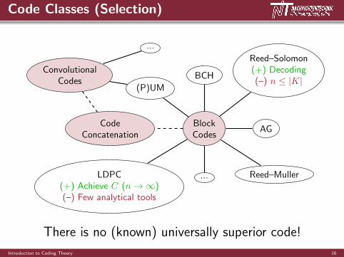
Code Classes (Selection)
ConvolutionalCodes
BlockCodes
...
...
Reed–Solomon(+) Decoding(–) n ≤ |K|
LDPC(+) Achieve C (n→∞)(–) Few analytical tools
BCH
AG
Reed–Muller
(P)UM
CodeConcatenation
There is no (known) universally superior code!
Introduction to Coding Theory 16

Code Classes (Selection)
ConvolutionalCodes
BlockCodes
...
...
Reed–Solomon(+) Decoding(–) n ≤ |K|
LDPC(+) Achieve C (n→∞)(–) Few analytical tools
BCH
AG
Reed–Muller
(P)UM
CodeConcatenation
There is no (known) universally superior code!
Introduction to Coding Theory 16

Code Classes (Selection)
ConvolutionalCodes
BlockCodes
...
...
Reed–Solomon(+) Decoding(–) n ≤ |K|
LDPC(+) Achieve C (n→∞)(–) Few analytical tools
BCH
AG
Reed–Muller
(P)UM
CodeConcatenation
There is no (known) universally superior code!
Introduction to Coding Theory 16

Code Classes (Selection)
ConvolutionalCodes
BlockCodes
...
...
Reed–Solomon(+) Decoding(–) n ≤ |K|
LDPC(+) Achieve C (n→∞)(–) Few analytical tools
BCH
AG
Reed–Muller
(P)UM
CodeConcatenation
There is no (known) universally superior code!
Introduction to Coding Theory 16

Code Classes (Selection)
ConvolutionalCodes
BlockCodes
...
...
Reed–Solomon(+) Decoding(–) n ≤ |K|
LDPC(+) Achieve C (n→∞)(–) Few analytical tools
BCH
AG
Reed–Muller
(P)UM
CodeConcatenation
There is no (known) universally superior code!
Introduction to Coding Theory 16

Code Classes (Selection)
ConvolutionalCodes
BlockCodes
...
...
Reed–Solomon(+) Decoding(–) n ≤ |K|
LDPC(+) Achieve C (n→∞)(–) Few analytical tools
BCH
AG
Reed–Muller
(P)UM
CodeConcatenation
There is no (known) universally superior code!
Introduction to Coding Theory 16
Code Classes (Selection)
ConvolutionalCodes
BlockCodes
...
...
Reed–Solomon(+) Decoding(–) n ≤ |K|
LDPC(+) Achieve C (n→∞)(–) Few analytical tools
BCH
AG
Reed–Muller
(P)UM
CodeConcatenation
There is no (known) universally superior code!
Introduction to Coding Theory 16

Outline
1 Code Constructions
2 Channels & Metrics
3 Decoding
4 Connection to Compressed Sensing
Introduction to Coding Theory 17

Channels
General
c P(r | c) r
Binary Symmetric Channel (0 < ε < 0.5)
0
1
0
1
1− ε
ε
ε
1− ε
ci
ei ∼ Ber(ε)
ri = ci + ei⊕⇐⇒
⇒ Hamming Metric
Introduction to Coding Theory 18

Channels
General
c P(r | c) r
Binary Symmetric Channel (0 < ε < 0.5)
0
1
0
1
1− ε
ε
ε
1− ε
ci
ei ∼ Ber(ε)
ri = ci + ei⊕⇐⇒
⇒ Hamming Metric
Introduction to Coding Theory 18

Channels
General
c P(r | c) r
Binary Symmetric Channel (0 < ε < 0.5)
0
1
0
1
1− ε
ε
ε
1− ε
ci
ei ∼ Ber(ε)
ri = ci + ei⊕⇐⇒
⇒ Hamming Metric
Introduction to Coding Theory 18

Channels
General
c P(r | c) r
Binary Symmetric Channel (0 < ε < 0.5)
0
1
0
1
1− ε
ε
ε
1− ε
ci
ei ∼ Ber(ε)
ri = ci + ei⊕⇐⇒
⇒ Hamming Metric
Introduction to Coding Theory 18
Channels
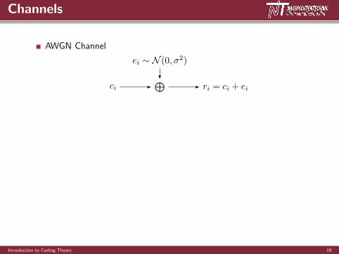
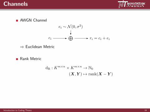
AWGN Channel
ci
ei ∼ N (0, σ2)
ri = ci + ei⊕
⇒ Euclidean Metric
Rank Metric
dR : Km×n ×Km×n → N0
(X,Y ) 7→ rank(X − Y )
Corresponding Channels
Random Linear Network CodingMIMO Transmission Systems
Introduction to Coding Theory 19

Channels
AWGN Channel
ci
ei ∼ N (0, σ2)
ri = ci + ei⊕
⇒ Euclidean Metric
Rank Metric
dR : Km×n ×Km×n → N0
(X,Y ) 7→ rank(X − Y )
Corresponding Channels
Random Linear Network CodingMIMO Transmission Systems
Introduction to Coding Theory 19
Channels
AWGN Channel
ci
ei ∼ N (0, σ2)
ri = ci + ei⊕
⇒ Euclidean Metric
Rank Metric
dR : Km×n ×Km×n → N0
(X,Y ) 7→ rank(X − Y )
Corresponding Channels
Random Linear Network CodingMIMO Transmission Systems
Introduction to Coding Theory 19

Channels
AWGN Channel
ci
ei ∼ N (0, σ2)
ri = ci + ei⊕
⇒ Euclidean Metric
Rank Metric
dR : Km×n ×Km×n → N0
(X,Y ) 7→ rank(X − Y )
Corresponding Channels
Random Linear Network CodingMIMO Transmission Systems
Introduction to Coding Theory 19

Outline
1 Code Constructions
2 Channels & Metrics
3 Decoding
4 Connection to Compressed Sensing
Introduction to Coding Theory 20

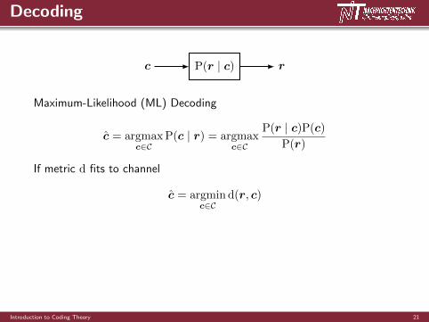
Decoding
c P(r | c) r
Maximum-Likelihood (ML) Decoding
c = argmaxc∈C
P(c | r) = argmaxc∈C
P(r | c)P(c)P(r)
If metric d fits to channel
c = argminc∈C
d(r, c)
In Practice
Convolutional Codes: ML-decodable (Viterbi Algorithm)
Block Codes: Often not ML-decodableE.g. C(400, 272, d) code over F2: |C| ≈ 1082
Introduction to Coding Theory 21

Bounded Minimum Distance Decoding
c1
c2
c3
c4
d
d2
r
Introduction to Coding Theory 22

Bounded Minimum Distance Decoding
c1
c2
c3
c4
d
d2
r
Introduction to Coding Theory 22

Bounded Minimum Distance Decoding
c1
c2
c3
c4
d
d2
r
Introduction to Coding Theory 22

Bounded Minimum Distance Decoding
c1
c2
c3
c4
d
d2
r
Introduction to Coding Theory 22

Bounded Minimum Distance Decoding
c1
c2
c3
c4
d
d2
r
Introduction to Coding Theory 22

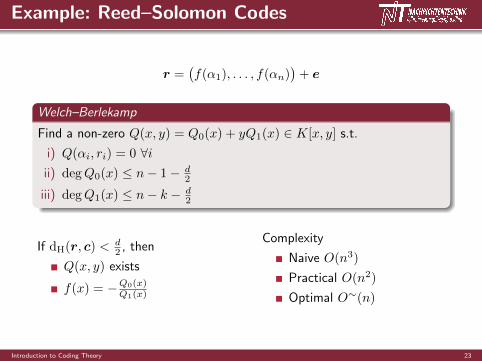
Example: Reed–Solomon Codes
r =(f(α1), . . . , f(αn)
)+ e
Welch–Berlekamp
Find a non-zero Q(x, y) = Q0(x) + yQ1(x) ∈ K[x, y] s.t.
i) Q(αi, ri) = 0 ∀iii) degQ0(x) ≤ n− 1− d
2
iii) degQ1(x) ≤ n− k − d2
If dH(r, c) <d2 , then
Q(x, y) exists
f(x) = −Q0(x)Q1(x)
Complexity
Naive O(n3)
Practical O(n2)
Optimal O∼(n)
Beyond d2?
Introduction to Coding Theory 23

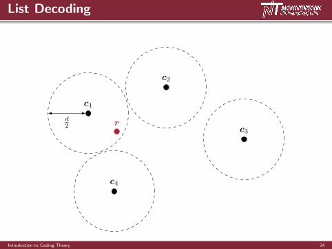
List Decoding
c1
c2
c3
c4
d2
rr
Introduction to Coding Theory 24
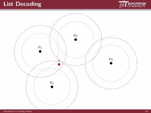
List Decoding
c1
c2
c3
c4
d2 r
r
Introduction to Coding Theory 24

List Decoding
c1
c2
c3
c4
d2 r
r
Introduction to Coding Theory 24
List Decoding
c1
c2
c3
c4
d2 r
r
Introduction to Coding Theory 24

List Decoding
c1
c2
c3
c4
d2 r
r
Introduction to Coding Theory 24

Outline
1 Code Constructions
2 Channels & Metrics
3 Decoding
4 Connection to Compressed Sensing
Introduction to Coding Theory 25

Connection to Compressed Sensing
Compressed Sensing (m� n)
Given b ∈ Cm,A ∈ Cm×n, find sparsest x ∈ Cn s.t.
b = Ax
Decoding Problem (n− k � n)
Given s ∈ Kn−k, H ∈ Kn−k×n, find e ∈ Kn of minimal wtH(e) s.t.
s = He
Solution:
Find some solution r = c+ e of
s = He = H(c+ e) = Hr.
Decode r −→ obtain c, e with minimal dH(r, c) = wtH(e)
Introduction to Coding Theory 26