introduction to compact (matrix) quantum groups and banica
TRANSCRIPT

Proc. Indian Acad. Sci. (Math. Sci.) Vol. 127, No. 5, November 2017, pp. 881–933.https://doi.org/10.1007/s12044-017-0362-3
© Indian Academy of Sciences 881
Introduction to compact (matrix) quantum groupsand Banica–Speicher (easy) quantum groups
MORITZ WEBER
Saarland University, Saarbrücken, GermanyE-mail: [email protected]
MS received 14 July 2017; published online 27 November 2017
Abstract. This is a transcript of a series of eight lectures, 90min each, held at IMScChennai, India from 5–24 January 2015. We give basic definitions, properties andexamples of compact quantum groups and compact matrix quantum groups such as theexistence of a Haar state, the representation theory and Woronowicz’s quantum versionof the Tannaka–Krein theorem. Building on this, we define Banica–Speicher quantumgroups (also called easy quantum groups), a class of compact matrix quantum groupsdetermined by the combinatorics of set partitions.We sketch the classification of Banica–Speicher quantum groups and we list some applications. We review the state-of-the-artregarding Banica–Speicher quantum groups and we list some open problems.
Keywords. Compact quantum groups; compact matrix quantum groups; easyquantum groups; Banica–Speicher quantum groups; noncrossing partitions; categoriesof partitions; tensor categories; Tannaka–Krein duality.
Mathematics Subject Classification. 20G42; 05A18; 46LXX.
1. Introduction
The study of symmetries in mathematics is almost as old as mathematics itself. Fromthe 19th century onwards, symmetries are mostly modelled by actions of groups. How-ever, modern mathematics requires an extension of the symmetry concept to highly non-commutative situations. This was the birth of quantum groups in the 1980’s; in the ICM1986 in Berkely, the notion ‘quantum group’ was coined by Drinfeld (see [82, Preface]),one of the pioneers together with Jimbo. See also the preface of Klimyk and Schmüdgen’sbook for more on the origins of quantum groups in quantum physics and why they shouldserve as ‘the concept of symmetry in physics’ [84, Preface].Also Woronowicz had applications to physics in mind when he introduced topological
quantum groups in 1987. In [132, Introduction], he writes that “in the existing theory (inphysics), it is known that the symmetry described by the considered group is broken”referring to elementary particle physics. We will follow his approach to quantum groups
This is a survey article on the emerging subject of Banica–Speicher quantum groups, based on a firstand extensive set of notes produced by Soumyashant Nayak of a lecture series in IMSc, Chennaiduring January 05–24, 2015.

882 Moritz Weber
based on the concept of ‘non-commutative function algebras’ by Gelfand–Naimark, usingC∗-algebras as our underlying algebras. The following illustrates Gelfand–Naimark’s phi-losophy of (topological) quantum spaces.
Topology Non-comm. topol.X comp. space ←→ C(X) cont. fcts. � AC∗-algebra
identif. (comm. C∗-alg.) f g �= g f (non-comm.).
Now, what are symmetries of such quantum spaces? In the same spirit, we should have
Comp. groups Comp. quantum groups.G comp. group ←→ C(G) cont. fcts. � AC∗-algebraG × G → G C(G) → C(G × G) � : A → A ⊗ A
.
In the first half of these lecture notes, we give the basic definitions, properties andexamples of compact quantum groups and compact matrix quantum groups such as theexistence of a Haar state, the representation theory and Woronowicz’s quantum version ofthe Tannaka–Krein theorem. See [86,87,95] for older surveys on compact quantumgroups,or [98,111] for more recent books. We do not cover the more general concept of locallycompact quantum groups of Kustermans and Vaes [88]. Moreover, we neglect algebraicquantum groups (which are based on the theory of Hopf algebras), see [82,84,94] formore on this, or [111] for some links and similarities between algebraic and topologicalperspectives on quantum groups.In the second half, we give an introduction to Banica–Speicher quantum groups [31],
also called easy quantum groups. They were defined in 2009 as a class of compact matrixquantum groups determined by the combinatorics of set partitions. The construction relieson Woronowicz’s Tannaka–Krein theorem, a quantum version of Schur–Weyl duality. Histheorem basically states that compact matrix quantum groups are in one-to-one correspon-dence to certain tensor categories. The idea behind Banica–Speicher quantum groups isnow to define a class of combinatorial objects which behaves like a tensor category and towhich we may actually associate one – which thus yields a quantum group by Tannaka–Krein duality. Thus, Banica–Speicher quantum groups are of a very combinatorial nature.To give a feeling for them, let us be slightly more precise. Consider a partition p of the
finite set {1, . . . , k, 1′, . . . , l ′} into disjoint subsets.We represent such partitions pictoriallyusing lines to represent the disjoint subsets.For instance, with k = 2 and l = 4,
p = { {1}, {2, 2′}, {1′}, {3′, 4′} }is represented as
2
2 3 4
∈ P (2, 4).
1
1
We associate a linear map
Tp : (Cn)⊗k → (Cn)⊗l
to such a partition p ∈ P(k, l).We then define operations on partitions, whichmatch nicelyvia the assignment p → Tp with tensor category like operations on the maps Tp (suchas forming the tensor product, the composition or the involution of linear maps). A class
CMQGs and Banica–Speicher quantum groups 883
of partitions which is closed under these operations is called a category of partitions; itthus induces a tensor category via p → Tp; and it thus induces a compact matrix quantumgroup via Tannaka–Krein, a Banica–Speicher quantum group. Summarizing
Combinatorics Comp. QGC categ. of part. � RC tensor categ. ←→ G BS QG
p partition p → Tp Tp linear map TK duality
We end the lectures by sketching the classification of Banica–Speicher quantum groupsand listing some applications.Moreover,we survey the state-of-the-art onBanica–Speicherquantum groups and we list several open problems. See [31,103,128] or the chapter [118,Ch. Easy quantum groups] for more on Banica–Speicher quantum groups.These lecture notes are a transcript of a series of eight lectures, 90min each, held at
IMSc, Chennai, India from 5–24 January 2015. For some of the proofs, details are leftout, as we tried to focus more on the motivation of definitions and concepts rather than oncomplete proofs. We assume the reader to be familiar with the basics of operator algebras,in particular, with the theory of C∗-algebras.
2. Definition and examples of CMQGs
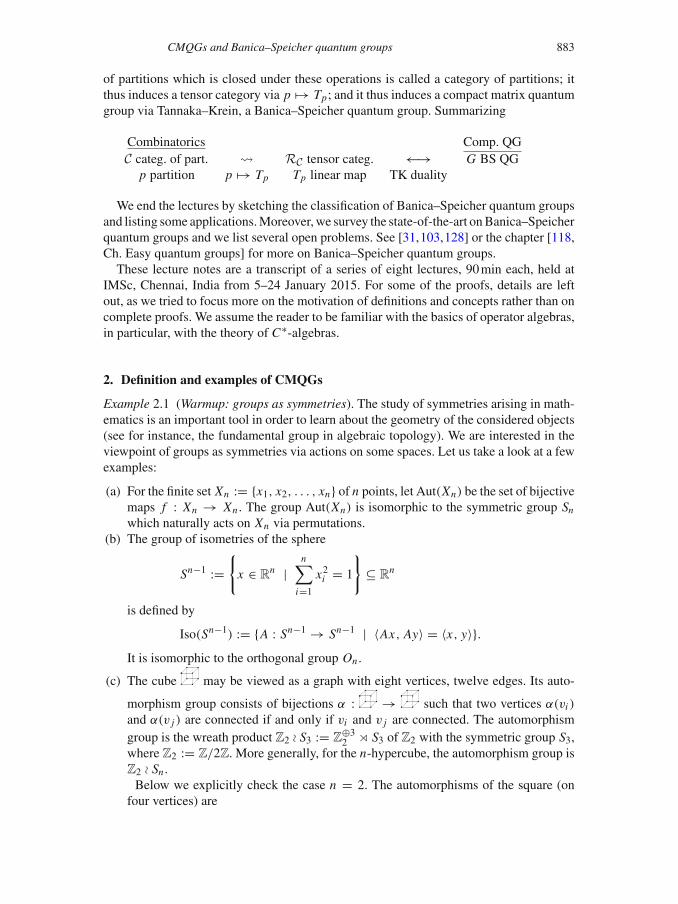
Example 2.1 (Warmup: groups as symmetries). The study of symmetries arising in math-ematics is an important tool in order to learn about the geometry of the considered objects(see for instance, the fundamental group in algebraic topology). We are interested in theviewpoint of groups as symmetries via actions on some spaces. Let us take a look at a fewexamples:
(a) For the finite set Xn := {x1, x2, . . . , xn} of n points, let Aut(Xn) be the set of bijectivemaps f : Xn → Xn . The group Aut(Xn) is isomorphic to the symmetric group Sn
which naturally acts on Xn via permutations.(b) The group of isometries of the sphere
Sn−1 :={
x ∈ Rn |
n∑i=1
x2i = 1
}⊆ R
n
is defined by
Iso(Sn−1) := {A : Sn−1 → Sn−1 | 〈Ax, Ay〉 = 〈x, y〉}.It is isomorphic to the orthogonal group On .
(c) The cube may be viewed as a graph with eight vertices, twelve edges. Its auto-
morphism group consists of bijections α : → such that two vertices α(vi )
and α(v j ) are connected if and only if vi and v j are connected. The automorphismgroup is the wreath product Z2 S3 := Z
⊕32 � S3 of Z2 with the symmetric group S3,
where Z2 := Z/2Z. More generally, for the n-hypercube, the automorphism group isZ2 Sn .Below we explicitly check the case n = 2. The automorphisms of the square (on
four vertices) are

884 Moritz Weber
e α β σ
αβσ αβ ασ βσ
The group
(Z2 ⊕ Z2) � S2 = 〈α, β, σ | α2 = β2 = e, αβ = βα, σ 2 = e, σασ
= β, σβσ = α〉has elements e, α, β, σ, αβσ, αβ, ασ, βσ and the above automorphisms fulfill therelations of (Z2 ⊕ Z2) � S2.
Note that the graph below has the same symmetry groupZ2 Sn as the n-hypercube.
· · · ·(2n vertices)
Reminder 2.2 (Basic facts in operator algebras). We want to study symmetries in anoperator algebraic context. To that end we review some basic ideas in operator algebras.They are a gateway to interpretations ofwhat a symmetry should be in the non-commutativecontext.
Philosophy behind non-commutative function algebras
AcompactHausdorff space X gives rise to a commutative unitalC∗-algebra, namelyC(X),the space of complex-valued continuous functions on X . Conversely, a commutative unitalC∗-algebra A is *-isomorphic to C(X), where
X := Spec(A) := {φ : A → C | φ is a *-homomorphism, φ �= 0}is a compact Hausdorff space (with theweak-∗ topology). Hence, wemay identify compacttopological spaces with commutative unitalC∗-algebras. Therefore, non-commutativeC∗-algebras may be viewed as non-commutative function algebras over ‘quantum spaces’, andthe theory of C∗-algebras turns into a ‘non-commutative topology’. See also [77, Ch. 1].Similarly a measure space (X, μ) may be uniquely identified with a commutative von
Neumann algebra, namely L∞(X, μ), the space of measurable bounded functions on Xacting by multiplication on the Hilbert space L2(X, μ). Thus, the study of von Neumannalgebras may be viewed as ‘non-commutative measure theory’.
Two equivalent definitions of C∗-algebras
C∗-algebras may be defined concretely as norm closed *-subalgebras of B(H), the set ofbounded linear operators on a Hilbert space H ; or abstractly as Banach algebras with aninvolution ‘*’ such that ‖a∗a‖ = ‖a‖2. The equivalence of the two definitions followsfrom the GNS construction.

CMQGs and Banica–Speicher quantum groups 885
Definition of universal C∗-algebras
The abstract definition of a C∗-algebra enables us to construct C∗-algebras in a purelyabstract way: as universal C∗-algebras. A universal C∗-algebra is prescribed by a set ofgenerators and relations which are realizable as bounded operators on a Hilbert space andenforce a uniform bound on the norm of the generators. We define a universal C∗-algebraas follows:
• Let E = {xi | i ∈ I } be a set of generators.• Let P(E) be the set of non-commutative polynomials in xi , x∗
i .• Let R ⊆ P(E) be a set of relations.• Let I(R) ⊆ P(E) be the ideal generated by the set of relations R.• Let A(E, R) := P(E)/I(R) be the quotient of P(E) by I(R); it is the universal
∗-algebra generated by E and R.• Let ‖x‖ := sup{p(x) | p be a C∗-seminorm on A(E, R)}; here p is aC∗-seminorm, if
p(λy) = |λ|p(x), p(x + y) ≤ p(x)+ p(y), p(xy) ≤ p(x)p(y) and p(x∗x) = p(x)2.• If for all x ∈ A(E, R), we have ‖x‖ < ∞, then we define C∗(E, R), the universal
C∗-algebra generated by E and R as the completion of
A(E, R)/{x | ‖x‖ = 0}in the norm ‖ · ‖.
Universal property of universal C∗-algebras
More important than the actual definition of a universalC∗-algebra is its universal property.If B is a C∗-algebra such that the elements {yi ∈ B | i ∈ I } satisfy the relations R, thenthere is a *-homomorphism, ϕ : C∗(E, R) → B such that ϕ(xi ) = yi .
Examples.
(i) The universal C∗-algebra C∗(u, 1 | u∗u = uu∗ = 1) is isomorphic to the algebraof continuous functions C(S1) on the sphere S1 ⊂ C.
(ii) A universal C∗-algebra C∗(x | x = x∗) does not exist as ‖x‖ is not finite.(iii) A universal C∗-algebra C∗(x, y | xy − yx = 1) does not exist as no two bounded
operators x, y can satisfy the relation xy − yx = 1.
Motivation 2.3 (Symmetries of quantum spaces?). Coming back to viewing C∗-algebrasas function algebras over ‘quantum spaces’ – what are symmetries of quantum spaces?Let us take a look at the classical case first, at symmetries of topological spaces, given byactions of groups.
Let X be a compact Hausdorff space, (G, ◦) be a compact group acting on X . In view ofthe machinery of Reminder 2.2, the first step is to pass to the algebras of functions (whichare commutative C∗-algebras). Indeed, an action
α : G × X → X
yields a *-homomorphism on the dual level (i.e. the level of function algebras)
α : C(X) → C(G × X) ∼= C(G) ⊗ C(X)
by composition. However, G is more than a topological space, it comes with a group law
◦ : G × G → G
(s, t) → s ◦ t.

886 Moritz Weber
Dualization of the group law gives us the following map:
� : C(G) → C(G × G) ∼= C(G) ⊗ C(G)
f → ((s, t) → f (s ◦ t)).
Here, we used the isomorphism
C(G × G) ∼= C(G) ⊗ C(G)
(s, t) → f (s)g(t) ↔ f ⊗ g.
Performing the second step of the machinery of Reminder 2.2, we shall now replaceC(G) andC(X) by possibly non-commutativeC∗-algebras A and B in order to have a non-commutative analog of a quantum space and its symmetry.Moreover, the dualization of thegroup law suggests that a quantum group should come with some map � : A → A ⊗ A.Note that, as C(G) is a nuclear C∗-algebra, we did not have to bother with what ⊗ pre-cisely means in this context, but in the general case, we will be interested in the minimaltensor product and may abuse notation by using ⊗ to mean ⊗min. See also Definition 2.8for more on actions.
DEFINITION 2.4 (Compact quantum group (CQG))
A compact quantum group (CQG) is a unital C∗-algebra A together with a unital*-homomorphism (the co-multiplication)
� : A → A ⊗min A,
such that
(� ⊗ id) ◦ � = (id⊗�) ◦ � (co-associativity),
and �(A)(1 ⊗ A) and �(A)(A ⊗ 1) are respectively dense in A ⊗min A. Here
�(A)(1 ⊗ A) := span{�(a)(1 ⊗ b) | a, b ∈ A}
and
�(A)(A ⊗ 1) := span{�(a)(b ⊗ 1) | a, b ∈ A}.
We also write A = C(G) in the spirit of Reminder 2.2 and we write G for the CQG. See[132,136] for the original definition.
Remark 2.5 (CQGs generalize compact groups).
(a) A quantum group is not a group!(b) If G is a compact group, then C(G) is a unital C∗-algebra and � is co-associative.
Indeed, we use associativity of G in order to show:
(� ⊗ id) ◦ �( f )(s, t, u) = �( f )((st), u)
= f ((st)u) = f (s(tu))
= (id⊗�) ◦ �( f )(s, t, u).

CMQGs and Banica–Speicher quantum groups 887
We verify it for�( f ) = f1⊗ f2 first and then it follows by taking linear combinations.The density condition of Definition 2.4 may also be verified easily. We infer that everycompact group is a CQG.
(c) Conversely, if (A,�) is a CQG such that A is commutative, then A is isomorphic toC(G) with G := Spec(A), and
� : C(G) → C(G) ⊗ C(G) ∼= C(G × G)
yields a map
m : G × G → G
by
m : Spec(A ⊗ A) → Spec(A)
ϕ → ϕ ◦ �.
It is a group law, hence G is a compact semigroup (co-associativity of � impliesassociativity of m). Now, what is the density condition in Definition 2.4 for?
Fact 1: If G is a compact semigroup such that the linear spaces �(C(G))(1⊗ C(G))
and �(C(G))(C(G) ⊗ 1) are respectively dense in C(G) ⊗ C(G), then G has can-cellation property (i.e. st = su ⇒ t = u).Fact 2: If G is a compact semigroup with cancellation property, then G is a group.
Hence, the density condition characterizes the step from semigroup to group and weinfer that G is a compact group.
(d) Summarizing, we conclude that CQGs generalize compact groups.
Example 2.6 (CQGs coming from group algebras). In order to see that CQGs are an honestgeneralization of compact groups, we shall come up with examples of CQGs (A,�) suchthat A is non-commutative. For doing so, let G be a discrete group.
(a) Recall the construction of the group C∗-algebra associated to G. The space
CG :=⎧⎨⎩∑g∈G
αgg finite linear combinations, αg ∈ C
⎫⎬⎭
is a *-algebra by(∑αgg) (∑
βhh)
:=∑
αgβh gh
and (∑αgg)∗ :=
∑αgg−1.
The abstract completion of CG with respect to the norm
‖x‖ := sup{‖π(x)‖ | π : CG → B(H)}yields a C∗-algebra denoted by C∗
max(G). It is isomorphic to the universal C∗-algebraC∗(ug, g ∈ G | ug unitary, uguh = ugh, u∗
g = ug−1).
As an example, verify that C∗(Z) = C(S1), see also the example in Reminder 2.2.The instance of ‖ · ‖ actually being a norm may be proven using the faithful map λ ofitem (b) below.

888 Moritz Weber
With
� : C∗max(G) → C∗
max(G) ⊗ C∗max(G)
given by the extension of
�(ug) := ug ⊗ ug
to C∗max(G), we have that (C∗
max(G),�) is a CQG. If G is non-abelian, then C∗max(G)
is non-commutative.(b) Likewise the reduced group C∗-algebra of G gives rise to a CQG. Recall that the left
regular representation of G,
λ : CG → B(2(G))
is defined by the linear extension of
λ(g)(δh) := δgh,
where (δh)h∈G is an orthonormal basis of the Hilbert space 2(G). As λ is faithful onCG, we know that λ(CG)) ⊆ B(2(G))) is isomorphic to CG. We may thus define
C∗red(G) := λ(CG) ⊆ B(2(G)))
as a concrete completion of CG, the reduced group C∗-algebra of G.Since the norm ‖ · ‖ in item (a) above is given by the supremum over all repre-
sentations, there is a natural map φ : C∗max(G) → C∗
red(G) and the comultiplicationmap
�red : C∗red(G) → C∗
red(G) ⊗ C∗red(G)
λ(g) → λ(g) ⊗ λ(g)
factorizes through φ, i.e. we have
�red ◦ φ = (φ ⊗ φ) ◦ �.
Hence, also (C∗red(G),�red) is a CQG.
We refer to [111, Ex. 5.1.2] for more details.
Motivation 2.7 (Dualizing actions of groups). Recall from Motivation 2.3 how to dualizethe action of a group. Let α : G × X → X be an action of a compact group G on a compactHausdorff topological space X . Thus, we obtain
α : C(X) → C(G × X) = C(G) ⊗ C(X)
f → f ◦ α.
It satisfies (id ⊗ α) ◦ α = (� ⊗ id ◦ α) (follows from g(hx) = (gh)x).
DEFINITION 2.8 ((Co-)action of a CQG)
An action (also called co-action) of a CQG (A,�) on a C∗-algebra B is a unital *-homomorphism α : B → A ⊗min B such that

CMQGs and Banica–Speicher quantum groups 889
(i) (id ⊗ α) ◦ α = (� ⊗ id) ◦ α,(ii) α(B)(A ⊗ 1) is linearly dense in A ⊗min B.
We may differentiate between left and right action. Some authors require slightly dif-ferent structures (like, modelling e · x = x), see for instance [124, Definition 2.1].
Example 2.9 (Quantum permutation group S+n ). The examples in Example 2.6 are CQGs
coming from classical groups. Let us now come to an honest quantum example.
Let Xn := {x1, · · · , xn} be a finite set of points. Then, its automorphism group Aut(Xn)
is exactly the permutation group Sn , see Example 2.1. Now, if we view Xn as a quantumspace – what is its quantum symmetry group? The first step is to dualize the set Xn andwe obtain
C(Xn) ∼= C∗(
p1, . . . , pn projections
∣∣∣∣n∑
i=1
pi = 1
).
Since the pi form a basis, any action of a CQG (A,�) on C(Xn) is of the form
α : C(Xn) → C(Xn) ⊗ A
p j →n∑
i=1
pi ⊗ ai j
for some elements ai j ∈ A. These elements ai j need to satisfy several relations:
α : C(Xn) → C(Xn) ⊗ A
p j →n∑
i=1
pi ⊗ ai j
for some elements ai j ∈ A. These elements ai j need to satisfy several relations:
α(p j ) = α(p j )∗ ⇒ai j = a∗
i j
α(p j ) = α(p j )2 ⇒∑
i
pi ⊗ ai j =∑k,i
pi pk ⊗ ai j ak j =∑
i
pi ⊗ a2i j
⇒ai j = a2i j
α is unital ⇒1 ⊗ 1 = α(1) = α
⎛⎝∑
j
p j
⎞⎠ =∑i, j
pi ⊗ ai j =∑
i
pi ⊗⎛⎝∑
j
ai j
⎞⎠
⇒∑
j
ai j = 1.
This led Wang [124] in 1998 to the definition
C(S+n ) := As(n) := C∗
(ui j , 1 ≤ i, j ≤ n | ui j projections,
∑k
uik =∑
k
uk j = 1
).
We may equip this C∗-algebra with a comultiplication � by putting
�(ui j ) := u′i j :=
∑k
uik ⊗ ukj .

890 Moritz Weber
Using the orthogonality of the projections uik and uil for k �= l (can be deduced from thefact that
∑k uik = 1), we check
u′2i j =∑k,l
uikuil ⊗ ukj ul j =∑
k
uik ⊗ ukj = u′i j
and ∑k
u′ik =∑
k
u′k j = 1 ⊗ 1.
Thus, by the universal property of C(S+n ), the map � is a *-homomorphism from C(S+
n )
to C(S+n ) ⊗ C(S+
n ) indeed. Moreover, it is co-associative due to
(� ⊗ id) ◦ �(ui j ) =∑
k
�(uik) ⊗ ukj
=∑k,l
uil ⊗ ulk ⊗ ukj
=∑
l
uil ⊗ �(ul j )
= (id ⊗ �) ◦ �(ui j ).
The density condition holds true, since
�(ui j )(1 ⊗ umj ) =∑
k
uik ⊗ ukj umj = uim ⊗ umj
implies
uim ⊗ 1 =∑
j
uim ⊗ umj ∈ �(A)(1 ⊗ A),
from which we may infer A ⊗ 1 ⊂ �(A)(1 ⊗ A), see also more details in Theorem 4.6.Similarly, we have 1 ⊗ umj ∈ �(A)(1 ⊗ A) and thus A ⊗ A = �(A)(1 ⊗ A).This shows that (C(S+
n ),�) is a CQG; actually, it is the quantum automorphism groupof Xn , see [124]. Thus, in the category of CQGs, the space Xn has more automorphisms:Its automorphism group is Sn in the category of groups, whereas it is S+
n in the categoryof CQGs.We may see that C(S+
n ) is non-commutative for n ≥ 4 due to the following argu-ment for n = 4. Consider a C∗-algebra B generated by two non-commuting projectionsp, q. By the universal property of the universal C∗-algebra C(S+
4 ), one may consider a*-homomorphism from C(S+
4 ) to B, which sends (ui j ) to the respective entries of thematrix below:⎛
⎜⎜⎝p 1 − p 0 0
1 − p p 0 00 0 q 1 − q0 0 1 − q q
⎞⎟⎟⎠ .
As B is non-commutative, C(S+4 ) must also be non-commutative. Thus S4 �= S+
4 .

CMQGs and Banica–Speicher quantum groups 891
Let us finish this example by remarking that C(Sn) is the abelinization of C(S+n ), i.e.:
C(S+n )/〈ui j ukl − uklui j 〉 ∼= C(Sn).
This can be proven by representing the symmetric group Sn ⊂ Mn(C) as permutationmatrices and then checking that the coordinate functions
ui j : Sn → C
g → gi j
satisfy the relations of C(S+n ). Using Stone–Weierstraß’s theorem, we infer that we have
a surjection from C(S+n ) to C(Sn) sending ui j to ui j . Moreover, the characters φ on
C(S+n )/〈ui j ukl −uklui j 〉 correspond exactly to permutation matrices and vice versa. Thus
Spec(C(S+n )/〈ui j ukl − uklui j 〉) ∼= Sn .
Comparing the comultiplication on C(Sn) arising as in Motivation 2.3, and making use ofthe fact that the multiplication of s, t ∈ Sn is simply given by matrix multiplication, weinfer
�(ui j )(s, t) = ui j (st) =∑
k
uik(s)uk j (t).
Under the natural isomorphism C(Sn × Sn) ∼= C(Sn) ⊗ C(Sn) as in Motivation 2.3, thisamounts to
�(ui j )(s, t) =(∑
k
uik ⊗ uk j
)(s, t),
in perfect analogy to the comultiplicationmap defined onC(S+n ). This proves that Sn ⊂ S+
nin the sense of the following definition.
DEFINITION 2.10 (Quantum subgroup)
(A,�A) is a quantum subgroup of (B,�B) if there is a surjection ϕ : B → A such that�A ◦ ϕ = (ϕ ⊗ ϕ) ◦ �B .
DEFINITION 2.11 (Compact matrix quantum group (CMQG))
Given n ∈ N, a compact matrix quantum group (CMQG) is defined as a pair (A, u) where
• A is a unital C∗-algebra which is generated by ui j ∈ A, 1 ≤ i, j ≤ n, the entries ofthe matrix u,
• u = (ui j ) and ut = (u ji ) are invertible,• and the map � : A → A ⊗min A defined by �(ui j ) = ∑k uik ⊗ ukj is a *-homomorphism.
Again, we write G for the CMQG in the sense of Remark 2.2 with C(G) = A a possiblynoncommutative C∗-algebra, see [132].
Remark 2.12 (CMQGs are CQGs). In Corollary 4.7, we will see that every CMQG is aCQG. In fact, the introduction of CMQGs predates one of CQGs. In 1987, Woronowiczdefined CMQGs under the name of ‘compact matrix pseudogroups’ [132]; in 1995, hedefined CQGs [136].

892 Moritz Weber
Example 2.13 (Orthogonal quantum group O+n ). In the same way we stepped from Sn to
S+n , we may define a quantum version of the orthogonal group On ⊆ Mn(C). Note that
C(On) can be written as a universal C∗-algebra, namely:
C(On) = C∗(ui j , 1 ≤ i, j ≤ n | ui j = u∗i j , u = (ui j ) is orthogonal,
ui j commute).
We may express the fact that u is orthogonal by the following relations:
∑k
uiku jk =∑
k
uki uk j = δi j .
In 1995, Wang [122] defined the free orthogonal quantum group O+n by.
C(O+n ) := Ao(n) := C∗(ui j , 1 ≤ i, j ≤ n|ui j = u∗
i j , u = (ui j ) is orthogonal).
It is easy to see that O+n is a CMQG containing On, S+
n and Sn as quantum subgroups.Hence, there are more quantum (orthogonal) rotations than classical ones. One can showthat O+
n is the quantum isometry group of the ‘quantum sphere’, [26, Theorem 7.2].
Wang and van Daele [115] (see also [124, Appendix] and the definition by Banica [2])also defined deformed versions of O+
n by
C(O+(Q)) := Ao(Q) := C∗(ui j , 1 ≤ i, j ≤ n|u unitary and u = QuQ−1).
Here Q ∈ GLn(C) such that Q Q = c1n, c ∈ R and u := (u∗i j ). Moreover, ui j �= u∗
i j ingeneral. For Q = 1n , we have O+(Q) = O+
n .
Example 2.14 (Unitary quantum group U+n ). The free unitary quantum group U+
n is theCMQG given by
C(U+n ) := Au(n) := C∗(ui j , 1 ≤ i, j ≤ n|u, ut unitary).
We may also write it as
C(U+n ) = C∗(ui j , 1 ≤ i, j ≤ n|u, u unitary)
revealing that C(O+n ) is nothing but the quotient of C(U+
n ) by u = u. Thus, O+n ⊂ U+
n .Moreover, the abelinization of C(U+
n ) is C(Un), so Un ⊂ U+n . Note that the requirement
of ut being unitary is automatic for commuting ui j , but not for non-commuting ones. Infact,
C∗(ui j , 1 ≤ i, j ≤ n|u unitary)
does not give rise to a CMQG as ut fails to be invertible [122, Example 4.1].

CMQGs and Banica–Speicher quantum groups 893
Again, there is a deformed version given by
C(U+(Q)) := C∗(ui j , 1 ≤ i, j ≤ n|u unitary and QuQ−1 unitary),
see [115,122].
Example 2.15 (Quantum special unitary group SUq(2)). Historically, Woronowicz’squantum version of SU (2) was the first example of a CQG. Recall
SU (2) := {u ∈ M2(C)|u unitary, det(u) = 1} ⊆ M2(C).
We may write SU (2) as
SU (2) ={(
a −cc a
) ∣∣∣ a, c ∈ C, |a|2 + |c|2 = 1
}.
For q ∈ [−1, 1]\{0}, we define SUq(2) as the CMQG given by
C∗(
α, γ
∣∣∣∣(
α −qγ ∗γ α∗
)is a unitary
).
Thus, its comultiplication is given by
�(α) = α ⊗ α − qγ ∗ ⊗ γ,�(γ ) = γ ⊗ α + α∗ ⊗ γ.
Moreover, we have [111, section 6.2]
SUq(2) ∼= O+(
0 1−q−1 0
),
see [133]. See also [134] for higher dimensional versions SUq(n).
Example 2.16 (Hyperoctahedral quantum group H+n ). Recall from Example 2.1(c) that
the hyperoctahedral group
Hn = Z2 Sn = 〈σ ∈ Sn, a1, . . . , an|a2i = e, ai a j = a j ai , σaiσ
−1 = aσ(i)〉
is the symmetry group of the n-hypercube and a certain graph. How to obtain a quantumversion of it? We first represent it as a matrix group:
Hn ∼= {(ui j ) orthogonal|uiku jk = uki uk j = 0 for i �= j} ⊂ On ⊂ Mn(C),
ai → a′i :=
⎛⎜⎜⎜⎜⎜⎜⎜⎜⎜⎜⎝
1. . .
1−1
1. . .
1
⎞⎟⎟⎟⎟⎟⎟⎟⎟⎟⎟⎠
.

894 Moritz Weber
To do so, check that {(ui j )| . . .} is a group indeed containing all matrices a′i and all per-
mutation matrices σ ; moreover, check that uiku jk = 0 implies that at most one entry perrow is nonzero; together with
∑i u2
ik = 1, this implies that this nonzero entry is either 1or −1; hence the group {(ui j ) | . . .} consists of all permutation matrices where any entry1 may be replaced by −1; all these matrices may be constructed in 〈a′
1, . . . , a′n, σ 〉.
This reveals that we should define the hyperoctahedral quantumgroup H+n as theCMQG
given by
C(H+n ) := C∗(ui j |ui j = u∗
i j , u orthogonal, uiku jk = uki uk j = 0, i �= j).
Note that the crucial step was to find a representation of Hn as a matrix group in termsof algebraic relations on the entries ui j . One can prove that H+
n is the quantum symmetrygroup of the graph as in Example 2.1(c); however, it is not the quantum symmetry groupof the n-hypercube. Actually, when Bichon [37] introduced H+
n in 2004, he also gave adefinition of a free wreath product ∗ with S+
n and he proved:
H+n = Z2 ∗ S+
n .
Finally, we have
S+n ⊂ H+
n ⊂ O+n and Hn ⊂ H+
n .
See also [15] for more on H+n .
Remark 2.17 (Locally compact quantum groups). There is a generalization of CQG tolocally compact quantum groups given by Kustermans and Vaes [88].
Remark 2.18 (Sources for examples of CQGs). The main approaches to obtain examplesof CQGs are:
(i) Liberation (‘let drop commutativity f g = g f ’), like S+n , O+
n , U+n , see [31,122,124,
128] amongst others.(ii) Deformation (‘deform commutativity: f g = qg f, q ∈ C’), like SUq(2), O(Q),
U+(Q), see [115,133] amongst others.(iii) Quantum isometry groups (‘quantum group of Riemannian isometries on a non-
commutative Riemannian manifold à la Connes’s non-commutative geometry’), see[26,35] amongst others.
In §5, we will elaborate more on the so-called Banica–Speicher quantum groups whichare CMQGs arising from (i).
3. The Haar state
Motivation 3.1 (Dualizing the Haar measure on groups). One very striking feature ofWoronowicz’s definition of a CQG is the existence of a Haar state dual to the Haar inte-gration for groups. Let us first consider the classical case.
Let G be a compact group. By Riesz’s theorem, there is a unique left-invariant Haarmeasure μG on G such that for all t ∈ G and all f ∈ C(G):∫
Gf (st) dμG(s) =
∫G
f (s) dμG(s).

CMQGs and Banica–Speicher quantum groups 895
Hence, we have a positive linear functional
h : C(G) → C
h →∫
Gf dμG
which remains invariant under left-translation:
(h ⊗ id) ◦ �( f )(t) =∫
G�( f )(s, t) dμG(s)
=∫
f (st) dμG(s)
=∫
f (s) dμG(s)
= h( f )1C(G)(t).
Having formulated the features of theHaar integration in ‘quantum terms’, i.e. as propertiesof the algebra C(G) – rather than as a characterization making use of elements g ∈ G –,we may now proceed to the quantum case and prove an analog of the Haar integration.
Theorem 3.2 (Existence of a Haar state). Let (A,�) be a compact quantum group. Thenthere is a unique state (the ‘Haar state’)
h : A → C
such that
(id ⊗ h) ◦ � = (h ⊗ id) ◦ � = h · 1A.
Proof. Define g ∗ h := (g ⊗ h) ◦ �, for g, h ∈ A′ (the space of continuous linearfunctionals on A) and a ∗ h := (id ⊗ h) ◦ �(a), for a ∈ A, h ∈ A′.
Uniqueness: If h′ is another such state, then
h′(a) = h(h′(a) · 1A) = h((id ⊗ h′) ◦ �(a))
= (h ⊗ h′) ◦ �(a) = h′((h ⊗ id) ◦ �(a)) = h(a).
Check h((id ⊗ h′) = h ⊗ h′ for �(a) = a1 ⊗ a2 and extend via linearity.
Existence: For ω ∈ A′ positive, we define
Kω := {ρ ∈ A′|ρ is a state, ρ ∗ ω = ω ∗ ρ = ω(1A)ρ}.
Then Kω is a closed subset (in the weak-* topology) of
(A′)+1 := {ρ ∈ A′ positive|‖ρ‖ ≤ 1}
and hence it is compact. We will prove the existence of a Haar state in the following threesteps:

896 Moritz Weber
(1) Kω �= ∅.(2) ∩n
i=1Kωi �= ∅, for all positive ωi ∈ A′, n ∈ N.(3) By Cantor’s intersection principle and (2), we may find a state h ∈ ∩ω∈(A′)+ Kω �= ∅.
It satisfies (id ⊗ h) ◦ � = (h ⊗ id) ◦ � = h.
Proof of (1). Let ω ∈ A′ be a state. Define ωn := 1n
∑nk=1 ω∗k where one inductively
defines ω∗(n+1) = ω ∗ (ω∗n) and ω∗1 = ω. As (A′)1 is compact, (ωn)n∈N has an accu-mulation point ρ. Since ‖ω ∗ ωn − ωn‖ = 1
n ‖ω∗(n+1) − ω‖ ≤ 2n , we have ω ∗ ρ = ρ.
Likewise ρ = ρ ∗ ω. This settles Kω �= ∅.Proof of (2). Let ω1, ω2 ∈ A′ be positive and define ω := ω1 +ω2. We only need to proveKω ⊆ Kω1 . Then ∅ �= Kω ⊆ Kω1 ∩ Kω2 and iteratively, ∅ �= K∑n
i=1 ωi⊆ ∩n
i=1Kωi .Assume that ω is a state. Let ρ ∈ Kω and define
Lρ⊗ω := {q ∈ A ⊗ A|(ρ ⊗ ω)(q∗q) = 0}.Then Lρ⊗ω ⊆ Lρ⊗ω1 since ω1 ≤ ω. Moreover Lρ⊗ω1 ⊆ Ker(ρ ⊗ ω1) by Cauchy–Schwarz. For ψL : A → A defined by ψL(a) := (id⊗ρ)�(a) − ρ(a)1, one can showthat (id⊗ψL)(�(A)) ⊆ Lρ⊗ω. Thus, keeping in mind that Lρ⊗ω is a left ideal, we have
1 ⊗ ψL(A) ⊆ (A ⊗ 1)(id⊗ψL)�(A) ⊆ (A ⊗ 1)Lρ⊗ω ⊆ Ker(ρ ⊗ ω1).
Hence
0 = (ρ ⊗ ω1)(1 ⊗ ψL(a)) = (ω1 ⊗ ρ)(�(a)) − ω1(1)ρ(a).
Thus ρ is in Kω1 .
Proof of (3). For h in ∩ω∈(A′)+ Kω, we have h ∗ ω = ω ∗ h = h for all states ω in A′. Fora ∈ A, let b := h(a) − (id⊗h)(�(a)) ∈ A. Then ω(b) = 0 for all states ω in A′. Thusb = 0.
We refer to [132, Thm. 4.2], [136, Thm. 2.3], [114] and [111, Thm. 5.1.6] for detailsregarding this proof. �
Remark 3.3 (Haar state not faithful). The Haar state is not always faithful. For instance,consider the CQG (C∗
max(G),�) given by a discrete group G, see also Example 2.6. TheHaar state hmax on C∗
max(G) is given by hmax(ug) = δg,e, since
(id⊗hmax)(�(ug) = ughmax(ug) = ueδg,e = 1δg,e = hmax(ug).
It is a tracial state i.e. hmax(ab) = hmax(ba) for all a, b in C∗max(G).
The Haar state hred on (C∗red(G),�) is given by hred(x) = 〈xδe, δe〉 as can be verified
directly. Now, the natural map φ : C∗max(G) → C∗
red(G) satisfies hmax = hred ◦ φ. Thushmax is not faithful in the case when φ is not an isomorphism (i.e. when G is not amenable).However, hred is always faithful on C∗
red(G).
DEFINITION 3.4 (Reduced version of a CQG)
Let G = (A,�) be a compact quantum group and h be its Haar state. The reduced versionof G is given by (Ared,�red) where Ared := πh(A) ⊆ B(Hh) (by the GNS construction

CMQGs and Banica–Speicher quantum groups 897
with respect to the Haar state h) and �red(πh(x)) := (πh ⊗ πh)(�(x)). One may alsoassociate to G the enveloping von Neumann algebra L(G) of Ared.
PROPOSITION 3.5 (Haar state of reduced version)
The comultiplication �red is well-defined and the Haar state on (Ared,�red) is given byhred(πh(x)) := h(x). It is faithful.
Proof. Let πh(x) = 0. Then h(x∗x) = 0. But then
(h ⊗ h)(�(x∗x)) = h((id⊗h)(�(x∗x))) = h(h(x∗x)1) = h(x∗x) = 0.
Thus �(x) ∈ Ker(πh⊗h) = Ker(πh ⊗ πh). We conclude that �red is well-defined. More-over,
(id⊗hred)�red(πh(x)) = (id⊗hred)(πh ⊗ πh)(�(x))
= πh(id⊗h)(�(x))
= πh(h(x)1)
= h(x)
= hred(πh(x)),
see also [98, Cor. 1.7.4]. �
DEFINITION 3.6 (Kac type)
A compact quantum group is said to be of Kac type if the Haar state is a trace.
Example 3.7 (Kac type CQGs). From Remark 3.3, we infer that (C∗max(G),�) and
(C∗red(G),�) are both of Kac type. See also Proposition 4.12 and Example 4.13 for more
on Kac type CQGs.
PROPOSITION 3.8 (Free product of CQGs)
Let (A,�A) and (B,�B) be CQGs. Then the free product is a CQG given by (A∗C B,�),where � is the extension of �A and �B arising from the universal property of the unitalfree product A ∗C B of the C∗-algebras A and B. The Haar state h on the free product isgiven by the free product (in the sense of free probability) of the Haar states h A and hB of(A,�A) and (B,�B), i.e.
(i) h ◦ i A = h A,(ii) h ◦ iB = hB,(iii) For all c1, · · · , cn ∈ A∪B ⊂ A∗CB such that h A(ci ) = 0 or hB(ci ) = 0 respectively
and ci , ci+1 come from different algebras, we have: h(c1 · · · cn) = 0.
Moreover, if (A,�A) and (B,�B) are CMQGs, so is their free product, see [122] and[111, Sect. 6.3].

898 Moritz Weber
PROPOSITION 3.9 (Tensor product)
Let (A,�A) and (B,�B) be CQGs. Then the tensor product is a CQG given by (A ⊗maxB, ρ ◦ (�A ⊗ �B)), where
ρ : (A ⊗min A) ⊗max (B ⊗min B) → (A ⊗max B) ⊗min (A ⊗max B).
Its Haar state is h A ⊗ hB and it is a CMQG if the original ones are, see [123] and [111,Sect. 6.3].
4. Representation theory and Tannaka–Krein
Motivation 4.1 (Representations of groups). Let G be a compact group and let U : G →B(H ) be a finite dimensional representation, i.e. dimH = m and U is continuous. ThenU ∈ C(G, Mm(C)) = C(G) ⊗ Mm(C), i.e.
U =∑α,β
uαβ ⊗ eαβ.
We have
U(gh) =∑α,β
uαβ(gh) ⊗ eαβ =∑α,β
�(uαβ)(g, h) ⊗ eαβ
and
U(g)U(h) =∑α,β
⎛⎝∑
γ
uαγ (g)uγβ(h)
⎞⎠⊗ eαβ.
Since U(gh) = U(g)U(h), by comparing the coefficients we have
�(uαβ)(g, h) =∑γ
uαγ (g)uγβ(h) =(∑
uαγ ⊗ uγβ
)(g, h).
Note that we used the isomorphism
C(G × G) ∼= C(G) ⊗ C(G)
in the last equality above. This motivates the following definition.
DEFINITION 4.2 (Representations of CQGs)
Let A be a unital C∗-algebra with a unital *-homomorphism � : A → A ⊗min A. A (finitedimensional) representation of (A,�) is a matrix u = (uαβ) ∈ Mm(A) such that
�(uαβ) =∑γ
uαγ ⊗ uγβ .

CMQGs and Banica–Speicher quantum groups 899
If the matrix has an inverse, then we call u non-degenerate and if it is unitary, we call it aunitary representation. If (A,�) is a CQG, this defines (finite dimensional) representationsfor CQGs. See also [95, Def. 3.5, Def. 5.1] for more on representations, including infinitedimensional ones.
DEFINITION 4.3 (Tensor products of representations)
Let u, v be two representations of a CQG (A,�), i.e.
u =∑
eαβ ⊗ uαβ ∈ Mn(u)(C) ⊗ A and
v =∑
eγ δ ⊗ vγ δ ∈ Mn(v)(C) ⊗ A.
Then we define
(a) u ⊗ v :=∑ eαβ ⊗ eγ δ ⊗ uαβvγ δ ∈ Mn(u)(C) ⊗ Mn(v)(C) ⊗ A.(b) u :=∑ eαβ ⊗ u∗
αβ.
DEFINITION 4.4 (Equivalence, irreducibility, intertwiners)
Let u ∈ B(Hu) ⊗ A and v ∈ B(Hv) ⊗ A be representations of a CQG (A,�).
(a) If a linear operator T ∈ B(Hu,Hv) is such that T u = vT , then T is called anintertwiner.
(b) The representations u and v are called equivalent, if there exists an intertwiner T ∈B(Hu,Hv) which is invertible.
(c) The representation v is called irreducible, if every intertwiner T u = uT is of the formT = λ · id.
PROPOSITION 4.5 (Irreducibility properties)
(a) If u is an irreducible representation, then u is irreducible.(b) If u is an irreducible unitary representation, then u is equivalent to a unitary repre-
sentation.
See [95, Lemma 6.9, Proposition 6.10].
Theorem 4.6 (Generation by coefficients of representations). Let A be a unital C∗-algebra with a unital *-homomorphism � : A → A ⊗min A.
(a) If A is generated (as a normed algebra) by the matrix elements of the nondegeneratefinite dimensional representations, then (A,�) is a CQG.
(b) If A is generated (as a C∗-algebra) by elements (uαβ) such that
�(uαβ) =∑
uαγ ⊗ uγβ
and u = (uαβ), ut = (uβα) are invertible, then (A,�) is a CQG.

900 Moritz Weber
Proof. We prove (a) first. Note that it suffices to check the co-associativity of � on thegenerators, but we have already checked co-associativity, see Example 2.9. Now let (wαβ)
be the inverse of some non-degenerate, finite dimensional representation (uαβ). Then
∑γ
�(uαγ )(1 ⊗ wγβ) =∑γ,ε
uαε ⊗ uεγ wγβ
=∑
ε
uαε ⊗ δεβ
= uαβ ⊗ 1 ∈ �(A)(1 ⊗ A).
holds.Next we show that a ⊗ 1, b ⊗ 1 ∈ �(A)(1 ⊗ A) implies ab ⊗ 1 ∈ �(A)(1 ⊗ A). We
holds take
a ⊗ 1 =∑γ
�(a1,γ )(1 ⊗ a2,γ )
and
b ⊗ 1 =∑
ε
�(b1,ε)(1 ⊗ b2,ε)
for some a1,γ , a2,γ , b1,γ , b2,γ ∈ A. Then we have
ab ⊗ 1 =∑γ
�(a1,γ )(1 ⊗ a2,γ )(b ⊗ 1)
=∑γ
�(a1,γ )(b ⊗ 1)(1 ⊗ a2,γ )
=∑γ,ε
�(a1,γ b1,ε)(1 ⊗ b2,εa2,γ )
and hence A ⊗ 1 ⊆ �(A)(1 ⊗ A) ⊆ A ⊗ A. Thus, if x ⊗ y ∈ A ⊗ A, we write
x ⊗ 1 =∑
i
�(ai )(1 ⊗ bi )
and we compute
x ⊗ y = (x ⊗ 1) (1 ⊗ y) =(∑
i
�(ai )(1 ⊗ bi )
)(1 ⊗ y)
=∑
i
�(ai )(1 ⊗ bi y) ∈ �(A)(1 ⊗ A).
This shows that A ⊗ A = �(A)(1 ⊗ A). Similarly we have that �(A)(1 ⊗ A) = A ⊗ A.This proves the density condition.

CMQGs and Banica–Speicher quantum groups 901
For part (b), note that u = (ut )∗ is invertible since ut is, and
�(u∗i j ) = �(ui j )
∗ =∑
k
u∗ik ⊗ u∗
k j .
Thus u, u are non-degenerate representations which generate A and we may use (a) toreach the conclusion. See also [95, Sect. 3]. �
COROLLARY 4.7 (CMQGs are CQGs)
Every compact matrix quantum group is a compact quantum group.
Proof. This is a immediate consequence of Theorem 4.6(b). �
Theorem 4.8 (Decomposition of representations).
(a) Every non-degenerate finite dimensional representation v is equivalent to a unitaryrepresentation.
(b) Every unitary representation decomposes into a direct sum of irreducible finite dimen-sional representations.
(c) The right regular representation contains all irreducible unitary representations.
Proof. For (a), let v be a non-degenerate finite dimensional representation and put
y := (id⊗h)(v∗v) ∈ Mm(C).
Note that v∗v is invertible, since v is invertible and as a positive, invertible element v∗v isstrictly positive, i.e v∗v > ε · 1 for some ε > 0. Then y ≥ 0 and in particular, y ≥ ε · 1,since the Haar state h is positive. Thus
ω := (y12 ⊗ 1)v(y− 1
2 ⊗ 1)
is a unitary representation equivalent to v. In order to check for instance ω∗ω = 1, verify
y ⊗ 1 = (id⊗h ⊗ id)(id⊗�)(v∗v) = v∗(y ⊗ 1)v.
As for (b), we consider the C∗-algebra of intertwiners
D = Hom (v, v).
We choose a maximal family (pn)n of pairwise orthogonal, minimal projections in D.Then one shows, using the fact that D acts non-degenerately on H , that
H ∼=⊕
pn H.
Finally the restriction of v to pn H is irreducible, since pn H is aminimal invariant subspace.For (c), we refer to [95]. �
902 Moritz Weber
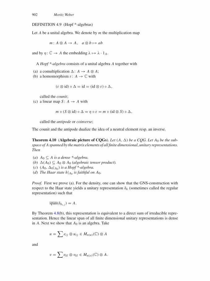
DEFINITION 4.9 (Hopf *-algebras)
Let A be a unital algebra. We denote by m the multiplication map
m : A ⊗ A → A, a ⊗ b → ab
and by η : C → A the embedding λ → λ · 1A.
A Hopf *-algebra consists of a unital algebra A together with
(a) a comultiplication � : A → A ⊗ A;(b) a homomorphism ε : A → C with
(ε ⊗ id) ◦ � = id = (id ⊗ ε) ◦ �,
called the counit;(c) a linear map S : A → A with
m ◦ (S ⊗ id) ◦ � = η ◦ ε = m ◦ (id ⊗ S) ◦ �,
called the antipode or coinverse;
The counit and the antipode dualize the idea of a neutral element resp. an inverse.
Theorem 4.10 (Algebraic picture of CQGs). Let (A,�) be a CQG. Let A0 be the sub-space of A spanned by the matrix elements of all finite dimensional,unitary representations.Then
(a) A0 ⊆ A is a dense *-algebra.(b) �(A0) ⊆ A0 ⊗ A0 (algebraic tensor product).(c) (A0,�0|A0) is a Hopf *-algebra.(d) The Haar state h|A0 is faithful on A0.
Proof. First we prove (a). For the density, one can show that the GNS-construction withrespect to the Haar state yields a unitary representation δh (sometimes called the regularrepresentation) such that
span(δhi, j ) = A.
By Theorem 4.8(b), this representation is equivalent to a direct sum of irreducible repre-sentation. Hence the linear span of all finite dimensional unitary representations is densein A. Next we show that A0 is an algebra. Take
u =∑
ei j ⊗ ui j ∈ Mn(u)(C) ⊗ A
and
v =∑
ekl ⊗ vkl ∈ Mn(v)(C) ⊗ A.

CMQGs and Banica–Speicher quantum groups 903
Then
u ⊗ v =∑
ei j ⊗ ekl ⊗ ui jvkl ∈ Mn(u)(C) ⊗ Mn(v)(C) ⊗ A.
This means, if ui j , vkl are the coefficients of the representation, their product are thecoefficients of the tensor product of the two representations. Showing that A0 is *-closedcan be done as in Theoreom 4.6(b).
Next we prove (b). It suffices to check that all monomials
uα1i1 j1
. . . uαkik jk
∈ A0
are mapped to A0 ⊗ A0. We have
�(
uα1i1 j1
. . . uαkik jk
)= �(
uα1i1 j1
). . . �
(uαk
ik jk
)=∑
γ1,...,γk
uα1i1γ1
. . . uαkikγk
⊗ uα1γ1 j1
. . . uαkγk jk
,
where each summand is contained in A0 ⊗ A0.For (c), we define the counit by
ε : A0 → C, ε(uαi j ) = δi j
and the antipode
S : A0 → A0, S(uαi j ) = (uα
j i )∗,
where uαi j are the coefficients of irreducible representations. It can be shown that they form
a basis for A0, thus ε and S are well-defined. Since A0 is spanned by all entries uαi j of
unitary representations uα , it suffices to check the properties of the counit, resp. antipode.We have
(ε ⊗ id)(�(uαi j )) =
∑k
ε(uαik)u
αk j =∑
k
δikuαk j = uα
i j
and
m((S ⊗ id)
(�(uα
i j )))
= m
((S ⊗ id)
(∑k
uαik ⊗ uα
k j
))
=∑
k
(uαik)
∗uαk j
= δi, j · 1= η(ε(uα
i j )),
and analogously the right counterparts.For part (d), we refer to [111, Sect. 5]. �

904 Moritz Weber
Remark 4.11 (Subtleties of the algebraic picture).
(a) The counit ε and antipode S are uniquely determined.(b) Theorem4.10 shows that we have a canonical ‘algebraic quantumgroup’ sitting inside
ourCQG.Conversely, startingwith aHopf*-algebra (A0,�),wemayassociate aCQG(A,�) to it such that A0 ⊆ A in the sense of the previous theorem.
(c) In general, the antipode on the C∗-algebra A need not be bounded. Thus, A might failto be a Hopf *-algebra itself. However, we will always find a dense Hopf *-algebraby Theorem 4.10.
See also [98, Sect. 1.6] and [113].
PROPOSITION 4.12 (Characterisations of Kac type CQGs)
Let (A,�) be a compact quantum group and let (A0,�0) be the Hopf *-algebra, S theantipode on A0. Then the following statements are equivalent:
(i) The Haar state is a trace (i.e. (A,�) is of Kac type in the sense of Definition 3.6).(ii) S2 = id.(iii) S is *-preserving.
A proof can be found in [98, Sect. 1.7.7], see also [84, Section 11.3].
Example 4.13 (Kac type and non-Kac type).
(a) S+n , O+
n , U+n are of Kac type using
ε : A → C, ε(ui j ) = δi j ,
S : A → A, S(ui j ) = u∗j i .
These maps exist by the universal properties of C(S+n ), C(O+
n ) and C(U+n ) respec-
tively.(b) SUq(2), O+
n (Q), U+n (Q) are not of Kac type, if Q∗Q �= 1.
ε : A → C, ε(ui j ) = δi j
S(ui j ) = u∗j i , S(u∗
i j ) =∑
(Q∗Q)−1il uml(Q∗Q)mj .
One sees that S is not *-preserving, hence these CQGs fail to be of Kac type. In fact,this was one of the main motivations for Woronowicz to introduce SUq(2). In hisphilosophy, Kac type CQGs are closer to the classical setting – note for instance thatCQGs arising as (C∗
red(G),�) are always of Kac type, see Example 3.7.
Remark 4.14 (Dual of a CQG).Wemay define the dual of a CQG (generalizing Pontryaginduality). Let (A,�) be a CQG, {uα : α ∈ I } mutually inequivalent unitary irreduciblerepresentations, A0 ⊆ A as before. Let B0 be the space of all linear functionals on A givenby x → h(ax), a ∈ A0. Then B0 is a subalgebra of A′ and isomorphic to the algebraicdirect sum⊕α∈I Mn(α)(C). Wemay define a comultiplication on B0 by using the multiplieralgebra of the algebraic tensor product B0⊗ B0. The completion yields a discrete quantumgroup which is by definition the dual quantum group.The Pontryagin duality tells us that a locally compact abelian group G may be recon-
structed from the information contained in its dual group of characters G. The classicalTannaka–Krein duality is an extension to compact non-abelian groups with the role of Gbeing replaced by its category of finite dimensional unitary representations. See also [63].

CMQGs and Banica–Speicher quantum groups 905
DEFINITION 4.15 (W*-category)
Let R be a set of objects equipped with a binary operation · : R × R → R. Let {Hr }r∈R
be a family of finite dimensional Hilbert spaces and for any r, s ∈ R, let Mor(r, s) be alinear subspace ofB(Hr ,Hs). Then (R, ·, {Hr }r∈R, {Mor(r, s)}r,s∈R) is called a concretemonoidal W*-category if the following conditions hold:
(i) For any r ∈ R, the identity operator idr acting on Hr belongs to Mor(r, r).(ii) If a ∈ Mor(r, r ′), b ∈ Mor(r ′, r ′′), then ba ∈ Mor(r, r ′′).(iii) For any r, s ∈ R and a ∈ Mor(r, s) we have a∗ ∈ Mor(s, r).(iv) IfHr = Hs and idr ∈ Mor(r, s), then r = s.(v) If a ∈ Mor(r, r ′) and b ∈ Mor(s, s′), then a ⊗ b ∈ Mor(r · s, r ′ · s′), for any
r, s, r ′, s′ ∈ R.(vi) For any p, r, s ∈ R: (p · r) · s = p · (r · s).(vii) There exists 1 ∈ R such that H1 = C, 1v = v1 = v.
A concrete monoidal W*-category (R, {Hr }r∈R, {Mor(r, s)}r,s∈R) is called complete ifthe following additional conditions hold:
(viii) For r ∈ R and any unitary v : Hr → K , where K is a Hilbert space, there existss ∈ R such that Hs = K and v ∈ Mor(r, s).
(ix) For r ∈ R and any orthogonal projection p ∈ Mor(r, r), there exists s ∈ R suchthat Hs = pHr and i ∈ Mor(s, r), where i is the embedding Hs → Hr .
(x) For r, r ′ ∈ R, there exists s ∈ R such that Hs = Hr ⊕ Hr ′ and the canonicalembeddings Hr → Hr ⊕ Hr ′ and Hr ′ → Hr ⊕ Hr ′ belong to Mor(r, s) andMor(r ′, s) respectively.
An element r ∈ R is said to be the complex conjugate of r ∈ R if there is an invertibleanti-linear map j : Hr → Hr such that the map
t j : C → Hr ⊗ Hr
defined by
t j (1) =∑
i
ei ⊗ j (ei )
is in Mor(1, r · r), and the map
t j : Hr ⊗ Hr → C
defined by
t j (eh ⊗ ei ) = 〈 j−1(eh), ei 〉
is in Mor(r · r, 1).
A finite subset Q of R is said to generate the W*-category, if for any s ∈ R, there aremorphisms bk ∈ Mor(q(k)
1 · · · q(k)nk , s), k = 1, 2, . . . , m for some q(k)
1 , q(k)2 , . . . , q(k)
nk ∈ Qsuch that
∑k bkb∗
k = ids ∈ Mor(s, s).

906 Moritz Weber
PROPOSITION 4.16 (Representations of a CQG form a W*-category)
Let G = (A, u) be a CMQG. Denote by RepG the set of all finite dimensional unitaryrepresentations of G and
Mor(v,w) := {T : Hv → Hw linear maps | T v = wT }
the space of intertwiners, where v ∈ B(Hv) ⊗ A and w ∈ B(Hw) ⊗ A. Then(Rep G,⊗, {Hr }r∈Rep G, {Mor(r, s)}r,s∈Rep G) forms a complete concrete monoidal W*-category. Furthermore for all v ∈ Rep G, there is v ∈ Rep G and {u, u} generatesRep G.
Proof. The proof is rather straightforward. Check for instance (v):
Tivi = wi Ti for i = 1, 2 �⇒ (T1 ⊗ T2)(v1 ⊗ v2) = (w1 ⊗ w2)(T1 ⊗ T2).
See also [134, Thm. 1.2]. �
DEFINITION 4.17 (Model of a W*-category)
Let (R, ·, {Hr }r∈R, {Mor(r, s)}r,s∈R) be a concrete monoidal W*-category generated by{ f, f }.(a) Let B be a unitalC∗-algebra and {vr }r∈R be a family of unitaries, i.e. vr ∈ B(Hr )⊗B.
Then M = (B, {vr }r∈R) is called a model of R if
(i) vr ·s = vr ⊗ vs .(ii) vr (t ⊗ 1) = (t ⊗ 1)vs for any r, s ∈ R and t ∈ Mor(s, r).
(b) Let B be a unital C∗-algebra and v be a unitary element of B(Hr ) ⊗ B. We say that(B, v) is an R-admissible pair if there exists a model M = (B, {vr }r∈R) such thatv f = v.
Theorem 4.18 (Tannaka–Krein for CMQGs). LetR = (R, ·, {Hr }r∈R, {Mor(r, s)}r,s∈R)
be a concrete monoidal W*-category such that { f, f } generates R. Then there is a CMQGG = (A, u) such that R = RepG, where R is the completion of R (in a natural sense).Moreover, G is universal in the following sense: if G ′ = (B, v) is a CMQG such thatR ⊆ RepG ′, there is a homomorphism A → B, u → v.
Sketch of the proof. At first, we assume that R is a complete concrete monoidal W*-category. Let Rirr be a complete set of mutually non-equivalent irreducible elements of Rwith 1R ∈ Rirr (there is such a set, because R is complete). Set
A :=⊕
α∈Rirr
B(Hα)′,
where B(Hα)′ is the space of linear functionals defined on B(Hα) for every α ∈ Rirr .For α ∈ Rirr and ρ ∈ B(Hα)′ the corresponding element of A will be denoted by uα
ρ .Therefore every a ∈ A can be written as finite sum
a =∑
α∈Rirr
uαρ.
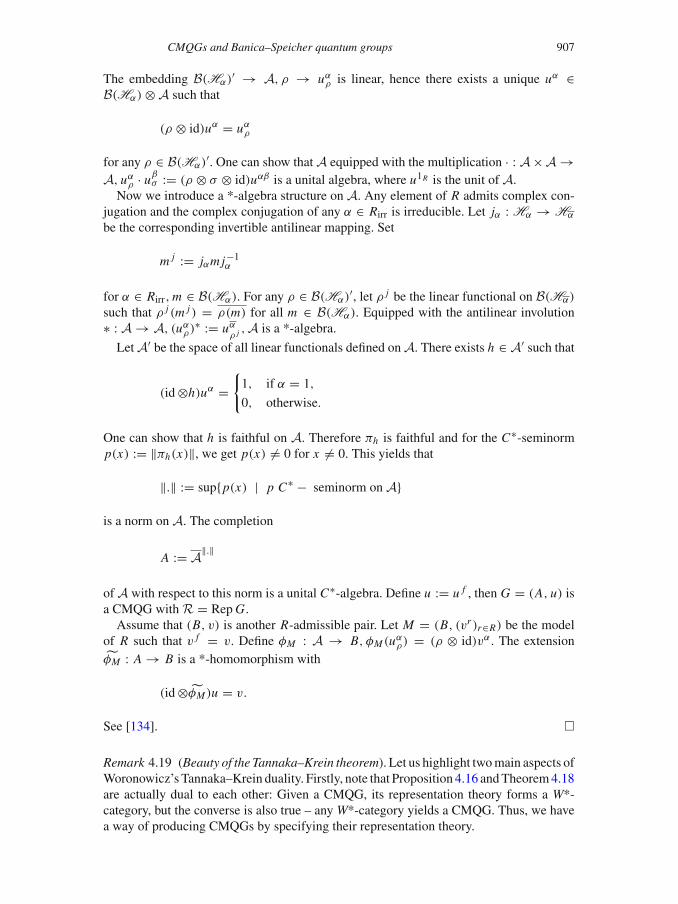
CMQGs and Banica–Speicher quantum groups 907
The embedding B(Hα)′ → A, ρ → uαρ is linear, hence there exists a unique uα ∈
B(Hα) ⊗ A such that
(ρ ⊗ id)uα = uαρ
for any ρ ∈ B(Hα)′. One can show thatA equipped with the multiplication · : A×A →A, uα
ρ · uβσ := (ρ ⊗ σ ⊗ id)uαβ is a unital algebra, where u1R is the unit of A.
Now we introduce a *-algebra structure on A. Any element of R admits complex con-jugation and the complex conjugation of any α ∈ Rirr is irreducible. Let jα : Hα → Hα
be the corresponding invertible antilinear mapping. Set
m j := jαmj−1α
for α ∈ Rirr, m ∈ B(Hα). For any ρ ∈ B(Hα)′, let ρ j be the linear functional on B(Hα)
such that ρ j (m j ) = ρ(m) for all m ∈ B(Hα). Equipped with the antilinear involution∗ : A → A, (uα
ρ)∗ := uαρ j ,A is a *-algebra.
LetA′ be the space of all linear functionals defined onA. There exists h ∈ A′ such that
(id⊗h)uα ={1, if α = 1,
0, otherwise.
One can show that h is faithful on A. Therefore πh is faithful and for the C∗-seminormp(x) := ‖πh(x)‖, we get p(x) �= 0 for x �= 0. This yields that
‖.‖ := sup{p(x) | p C∗ − seminorm on A}
is a norm on A. The completion
A := A‖.‖
ofA with respect to this norm is a unital C∗-algebra. Define u := u f , then G = (A, u) isa CMQG withR = RepG.Assume that (B, v) is another R-admissible pair. Let M = (B, (vr )r∈R) be the model
of R such that v f = v. Define φM : A → B, φM (uαρ) = (ρ ⊗ id)vα . The extension
φM : A → B is a *-homomorphism with
(id⊗φM )u = v.
See [134]. �
Remark 4.19 (Beauty of the Tannaka–Krein theorem). Let us highlight twomain aspects ofWoronowicz’s Tannaka–Krein duality. Firstly, note that Proposition 4.16 andTheorem4.18are actually dual to each other: Given a CMQG, its representation theory forms a W*-category, but the converse is also true – any W*-category yields a CMQG. Thus, we havea way of producing CMQGs by specifying their representation theory.

908 Moritz Weber
The second aspect is more subtle. Note that for Theorem 4.18, we did not require theW*-category R to be complete. Thus, we do not need to specify the whole representationtheory of a CMQG, we only need to come up with parts of it. This is a drastic reductionof complexity from which we will profit in the next chapter.See also [110] (or rather the appendix [108] in the arxiv version of this article) for more
on the interpretation of the Tannaka–iKrein theorem.
5. From Tannaka–Krein to Banica–Speicher quantum groups
DEFINITION 5.1 (Categories of partitions)
(a) A partition p ∈ P(k, l) is a decomposition of k + l points (k of which are ‘upper’,l ‘lower’) into disjoint subsets called the blocks. We illustrate examples of partitionspictorially below:
2
2 3 4
∈ P (2, 4),
1
1
1 2 3 4
1
∈ P (4, 1).
The set of all partitions {P(k, l) : k, l ∈ N0} is denoted byP .(b) Let p ∈ P(k, l), q ∈ P(k′, l ′), then their tensor product p ⊗ q ∈ P(k + k′, l + l ′) is
the partition obtained by placing p and q side-by-side. Pictorially,
⊗ =
(∈ P (2, 4))) (∈ P (4, 1)) (∈ P (6, 5))
(c) Let p ∈ P(k, l), q ∈ P(l, m), the composition qp ∈ P(k, m) is the partition obtainedby aligning the lower points of p right above the upper points of q and ignoring thel middle points so obtained. Certain loops/blocks may appear purely in the middlewith no connections to the points in the upper or lower ends of the aligned partitionsand are removed. They are referred to as removed blocks. Pictorially
(∈ P (2, 4))
(∈ P (4, 1))
= (∈ P (2, 1)).

CMQGs and Banica–Speicher quantum groups 909
(d) If p ∈ P(k, l), then the involution p∗ ∈ P(l, k) is the partition obtained by turning pupside down. Pictorially,
∗=
(∈ P (4, 1))
(∈ P (1, 4))
(e) A subset C ⊆ P (consisting of sets C(k, l) ⊆ P(k, l)) is a category of partitionsif it is closed under (b), (c), (d) and if the identity partition | ∈ P(1, 1) and the pairpartition ∈ P(0, 2) are both in C . See [31].
Example 5.2 (Categories of partitions).
(a) P is a category of partitions.(b) The set NC of all non-crossing partitions (i.e. the lines linking the various points
in the partition may be drawn in such a way that they do not cross) is a category of
partitions. The partition ∈ P(3, 2) is an example of a non-crossing partitionwhereas the partition ∈ P(2, 2) is an example of a partition with crossings.
(c) The setP2 of all pair partitions (all blocks are of size two) is a category of partitions.(d) The set NC2 := P2∩NC of all non-crossing pair partitions is a category of partitions.
DEFINITION 5.3 (Linear maps associated to partitions)
Let p ∈ P(k, l) and let n ∈ N be a fixed natural number. Define
Tp : (Cn)⊗k → (Cn)⊗l
as the linear map given by
Tp(ei1 ⊗ · · · ⊗ eik ) :=∑
j1,··· , jl
δp(i, j)e j1 ⊗ · · · ⊗ e jl ,
where i = (i1, . . . , ik) ∈ {1, 2, . . . , n}k and j = ( j1, . . . , jl) ∈ {1, 2, . . . , n}l are multi-ndices and (ei )i=1,...,n is the canonical orthonormal basis of C
n . Moreover, δp(i, j) isdefined as follows: Label the upper points in the partition p with i1, . . . , ik and the lowerpoints with j1, . . . , jl . Then δp(i, j) = 1 if the partition p connects only equal-valued
indices, and 0 otherwise. For example, consider the partition p := ∈ P(4, 1). Ifi = (1, 3, 4, 4), j = (1), then δp(i, j) = 0 as can be seen from the picture below:
1 3 4 4
1

910 Moritz Weber
Similarly if i = (1, 1, 4, 4), j = (1), then δp(i, j) = 1 as can be seen below:
1 1 4 4
1
Example 5.4 (Linear maps associated to partitions).
(a) For the partition p = ∈ P(2, 2), we have
Tp(ei1 ⊗ ei2) = ei2 ⊗ ei1 .
This is because δp(i, j) = 1 if and only if j can be obtained by flipping the indicesin i . This may be deduced from the picture below:
i1 i2
j1 j2 .(b) For p =|∈ P(1, 1), we note that Tp is the identity map.
PROPOSITION 5.5 (Operations on partitions pass to linear maps)
If p, q are partitions in P , then
(a) Tp ⊗ Tq = Tp⊗q .(b) Tq Tp = nα(q,p)Tqp, where α(q, p) denotes the number of removed blocks in the
composition. Note that p and q need to have appropriate sizes in order to performthe composition.
(c) (Tp)∗ = Tp∗
Proof.
(a) Let p ∈ P(k, l) and q ∈ P(k′, l ′). Since the partition p⊗q is obtained by concatenatingp and q, we have δp⊗q(i ⊗ i ′, j ⊗ j ′) = δp(i, j) · δq(i ′, j ′) (where the suggestive notationi ⊗ i ′ denotes the concatenation of the labelling sets i and i ′.)
Unwrapping the definitions of Tp, Tq , Tp ⊗ Tq , Tp⊗q , we see that
(Tp ⊗ Tq)(ei1 ⊗ · · · ⊗ eik ⊗ ei ′1 ⊗ · · · ⊗ ei ′k′ )
= Tp(ei1 ⊗ · · · ⊗ eik ) ⊗ Tq(ei ′1 ⊗ · · · ⊗ ei ′k′ )
=∑j, j ′
δp(i, j)(e j1 ⊗ · · · ⊗ e jl ) ⊗ δq(i ′, j ′)(e j ′1 ⊗ · · · ⊗ e j ′l′)
=∑j, j ′
δp(i, j) · δq(i ′, j ′)(e j1 ⊗ · · · ⊗ e jl ⊗ e j ′1 ⊗ · · · ⊗ e j ′l′)
=∑j, j ′
δp⊗q(i ⊗ i ′, j ⊗ j ′)(e j1 ⊗ · · · ⊗ e jl ⊗ e j ′1 ⊗ · · · ⊗ e j ′l′)
= Tp⊗q(ei1 ⊗ · · · ⊗ eik ⊗ ei ′1 ⊗ · · · ⊗ ei ′k′ ).

CMQGs and Banica–Speicher quantum groups 911
Thus we conclude that Tp ⊗ Tq = Tp⊗q .(b) Let p ∈ P(k, l) and q ∈ P(l, m). Then
Tq Tp(ei1 ⊗ · · · ⊗ eik ) =∑
j
δp(i, j)Tq(e j1 ⊗ · · · ⊗ e jl )
=∑
h
⎛⎝∑
j
δp(i, j) · δq( j, h)
⎞⎠ (eh1 ⊗ · · · ⊗ ehm ).
From the above calculation, as the coefficient of eh1 ⊗· · ·⊗ehm is∑
j δp(i, j) ·δq( j, h),
we take a closer look at the terms δp(i, j) · δq( j, h) for different choices of the labellingset j to identify the origin of the scaling term nα(p,q).Wehave that δqp(i, h) = 1 if and only if the alignment of p andq to form the composition
qp connects equal-valued indices in i and h.Let δqp(i, h) = 1. We try to find all possible values of indices in j for which δp(i, j) ·
δq( j, h) = 1. As the removed blocks arise when blocks purely in the lower part of p arealigned to blocks purely in the upper part of q, the value of the indices in j that correspondto the removed block must all be equal. Thus each removed block gives rise to n choicesfor the common value of the indices of j in that block. The values of the remaining indicesof j for which δp(i, j) · δq( j, h) = 1 are uniquely determined by their connections to theupper part in p and to the lower part in q. Hence, whenever δqp(i, h) = 1, we have that∑
j δp(i, j) · δq( j, h) = nα(q,p).
If δp(i, j) = 1 and δq( j, h) = 1 for some j , then δqp(i, h) = 1. Thus if δqp(i, h) = 0,we have that for any j , either δp(i, j) = 0 or δq( j, h) = 0. As a result
∑j δp(i, j) ·
δq( j, h) = 0.Summing up the above conclusions, we conclude that
nα(q,p)δqp(i, h) =∑
j
δp(i, j) · δq( j, h)
holds for all i, h.Thus Tq Tp = nα(q,p)Tqp.
(c) Let p ∈ P(k, l). Note that
δp∗( j, i) = 〈ei1 ⊗ · · · ⊗ eik , Tp∗(e j1 ⊗ · · · ⊗ e jl )〉,δp(i, j) = 〈Tp(ei1 ⊗ · · · ⊗ eik ), e j1 ⊗ · · · ⊗ e jl 〉
= 〈ei1 ⊗ · · · ⊗ eik , T ∗p (e j1 ⊗ · · · ⊗ e jl )〉.
As the partition p∗ is obtained by turning p upside down,we see that δp∗( j, i) = δp(i, j)and thus
〈ei1 ⊗ · · · ⊗ eik , Tp∗(e j1 ⊗ · · · ⊗ e jl )〉 = 〈ei1 ⊗ · · · ⊗ eik , T ∗p (e j1 ⊗ · · · ⊗ e jl )〉
for all i, j . From this, we conclude that T ∗p = Tp∗ . See [31]. �

912 Moritz Weber
We illustrate how α(q, p) arises in part (b) of Proposition 5.5 with an example. Let
p = and q = . Then
Tq Tp(ei1 ⊗ ei2) =∑h1
⎛⎝ ∑
j1,..., j4
δp(i, j)δq( j, h)
⎞⎠ eh1 .
Looking at the picture below,
i2
j2 j3 j4
j1 j2 j3 j4
h1
i1
j1
it is clear that the non-zero coefficients arise in the sum∑
j1,..., j4 δp(i, j)δq( j, h) when
δp(i, j) = δq( j, h) = 1, which holds when j2 = i2 = j1 = h1 and j3 = j4. ThusTq Tp(ei1 ⊗ ei2) = nδqp(i, s) (as there are n arbitrary choices for j3(= j4)).
DEFINITION 5.6 (Banica–Speicher quantum groups)
A CMQG G is called a Banica–Speicher QG, if Sn ⊆ G ⊆ O+n and if there is a category
of partitions C ⊆ P such that
Mor(u⊗k, u⊗l) = span{Tp | p ∈ C(k, l)}
for all k, l ∈ N0. It is called free, ifC ⊆ NC . An alternative name (in the past few years, thealternative name came up in order to honor the two pioneers in the theory of easy quantumgroups, and also to avoid confusion with the common meaning of the word ‘easy’ in thesense of ‘not difficult’) for Banica–Speicher quantum groups (in fact the original one) iseasy quantum groups. See [31].
Remark 5.7 (Tracing back Banica–Speicher QGs to Tannaka–Krein). The definition ofBanica–Speicher quantum groups is based on the Tannaka–Krein Theorem 4.18. Let usmake this more precise in the sequel. We also refer to [108].
PROPOSITION 5.8 (From categories of partitions to W*-categories)
Let C ⊆ P be a category of partitions and let n ∈ N. We put
• R := N0 with the binary operation r · s := r + s.• Hr := C
n for r ∈ R, with H0 := C.• Mor(r, s) := span{Tp | p ∈ C(r, s)}
This defines a concrete W*-category R generated by 1 = 1.

CMQGs and Banica–Speicher quantum groups 913
Proof. It is straightforward to check the axioms of a concrete W*-category. Moreover,1 = 1 since j : C
n → Cn defined by j (
∑αi ei ) = ∑αi ei yields t j (1) = ∑ ei ⊗ ei =
Tp(1), Tp ∈ Mor(0, 2) and t j (ei1 ⊗ei2) = δi1,i2 = Tp∗(ei1 ⊗ei2), Tp∗ ∈ Mor(2, 0),wherep is the pair partition . Finally, {1} generates R, since 1 + · · · + 1(k times) = k; fork ∈ N0, take m = 1, b1 = idk ∈ Mor(k, k). �
COROLLARY 5.9 (From Tannaka–Krein to Banica–Speicher QGs)
Given a category of partitions C and n ∈ N, we obtain a CMQG G = (A, u) by Proposi-tion 5.8 and Theorem 4.18. It is a Banica–Speicher quantum group with Sn ⊆ G ⊆ O+
n .More precisely,
(a) (A, (u⊗r )r∈N0) is a model of the W*-category of Proposition 5.8 with u = u, u(r ·s) =ur ⊗ us and T u⊗r = u⊗s T for all r, s ∈ R and T ∈ Mor(r, s). In particular,
Tpu⊗k = u⊗l Tp
for all p ∈ C(k, l).(b) A is the smallest C∗-algebra containing the matrix elements of u and it is universal, i.e.
if (B, u′) is another model of the above W*-category, then there is a homomorphismfrom A to B which carries u to u′.
Remark 5.10 (Banica–Speicher QGs defined by relations). From Corollary 5.9, we knowthat A is a universal C∗-algebra generated by elements ui j , 1 ≤ i, j ≤ n with ui j = u∗
i j
satisfying the relations Tpu⊗k = u⊗l Tp for partitions p ∈ C(k, l).As
u⊗k(ei1 ⊗ · · · ⊗ eik ⊗ 1) =∑
t
et1 ⊗ · · · ⊗ etk ⊗ ut1i1 · · · utk ik ,
we infer
Tpu⊗k(ei1 ⊗ · · · ⊗ eik ⊗ 1) =∑
t1,...,tk
Tp(et1 ⊗ · · · ⊗ etk ) ⊗ ut1i1 · · · utk ik
=∑
s1,...,sl
es1 ⊗ · · · ⊗ esl
⊗( ∑
t1,...,tk
δp(t, s)ut1i1 · · · utk ik
)
as well as
u⊗l Tp(ei1 ⊗ · · · ⊗ eik ⊗ 1) =∑
s1,...,sl
es1 ⊗ · · · ⊗ esl
⊗⎛⎝ ∑
j1,..., jl
δp(i, j)us1 j1 · · · usl jl
⎞⎠ .

914 Moritz Weber
Comparing coefficients, we have the following set of relations in A if and only if Tpu⊗k =u⊗l Tp: ∑
t1,...,tk
δp(t, s)ut1i1 · · · utk ik =∑
j1,..., jl
δp(i, j)us1 j1 · · · usl jl , for any s, i .
Example 5.11 (Relations coming from partitions). Below we consider examples of rela-tions in A we may obtain by analysing various partitions using Remark 5.10.
(a) Let . We get
δs1s21A = δp(0, s1s2)1A =∑j1, j2
δp(0, j1 j2)us1 j1us2 j2 =∑
j1
us1 j1us2 j1 .
Thus, we get the relation uut = 1Mn(A).
(b) Let p := ∈ P (0, 1). We note that δp(0, s1)1A = ∑ j1 δp(0, j1)us1 j1 . The relations
we get are∑
k uik = 1A for all i ∈ {1, 2, . . . , n}.
(c) Let p := ∈ P (2, 2). This partition gives relations of the form uiku jk = uki uk j = 0
if i �= j .(d) Let p := ∈ P(2, 2). We conclude that ui j ukl = uklui j for all i, j, k, l ∈
{1, 2, . . . , n} which means A is commutative.
Remark 5.12 (S+n and O+
n are Banica–Speicher QGs). From the above examples, wededuce that if G ′ = (A′, u′) is associated to the category of non-crossing partitions NCin the sense of Definition 5.6 and Corollary 5.9, there is a homomorphism from C(S+
n ) toA′. One may check that in C(S+
n ) all relations corresponding to NC are fulfilled. Thus weconclude that S+
n is isomorphic to G ′ and hence it is a Banica–Speicher quantum group.Similarly, from the additional commutativity relations obtained from the crossing partitionin (d), we see that the group Sn may be associated with the category of all partitions P .Further,P2 may be associated with the orthogonal group On and NC2 may be associatedwith O+
n in the sense of Defiinition 5.6 and Corollary 5.9 and they are all Banica–Speicherquantum groups.
Since for all categories of partitionsC wehave NC2 ⊆ C ⊆ P , we infer that Sn ⊆ G ⊆O+
n holds for all Banica–Speicher quantum groups G (i.e. C(Sn) � C(G) � C(O+n )
mapping generators to generators).Summarizing, we have the following one-to-one correspondence:
Combinatorics CMQGsCategories of partitions ←→ Banica–Speicher QGs.
See also [31,103,128,130] for more on Banica–Speicher quantum groups.
6. Classification of Banica–Speicher quantum groups
Lemma 6.1 (Rotation invariance). Any category C ⊆ P of partitions is closed underrotation, i.e. if p ∈ P(k, l) is in C , then so is the partition obtained by shifting the left-most upper point to the left of all lower points, and similarly by moving the right-most

CMQGs and Banica–Speicher quantum groups 915
upper point to the right of all lower points, and also under the reverse operations. We
illustrate the rotation operation with the following examples: Let ∈ C . If we perform
a left-rotation, the above lemma says that ∈ C . Similarly a further right-rotation
gives us that is in C . We may play around with both operations to conclude thatis also in C .
Proof. Let p ∈ P(k, l) be a partition in C . As C is a category, it contains the identitypartition |, the pair partition and thus contains p1 :=| ⊗ p and p2 := ⊗ |⊗(k−1).In order to do the left rotation manoeuvre, we compose p1 ∈ P(k + 1, l + 1) withp2 ∈ P(k − 1, k + 1) to get an element p1 p2 of P(k − 1, l + 1). Pictorially:
· · ·
p .⊗
Thus the composition yields a left rotation as described in the lemma. Similarly the closureof C under the other rotation operations may be proved by suitable choices of p1, p2 asabove. See [31]. �
Lemma 6.2 (Generators of categories). Let 〈p1, . . . , pn〉 denote the smallest categorywhich contains p1, . . . , pn ∈ P . We describe generating sets for different categories ofpartitions:(a) NC2 = 〈∅〉,(b) P2 = 〈 〉,(c) NC = 〈 , 〉,(d) P = 〈 , , 〉.Keeping in mind that we always have the identity partition | and the pair partition in acategory of partitions C , we omit to write them down in the list of generators.
Proof. Before proceeding forward, we make a few useful observations in order to stream-line the proof.
(i) For a partition in a category C ⊆ P with k upper points and l lower points, one mayperform k left-rotations to obtain an element of C with no upper points and k + llower points. Keeping in mind that the process is reversible, all we need to check isthat the generating set for C generates all elements of C(0, n) for all n ∈ N.
(ii) Let p ∈ NC(0, n). In general, as p is a non-crossing partition with only lower points,it looks like
· · ·· · ·· · ·
· · ·
· · ·· · ·

916 Moritz Weber
Using a minimality argument for block size, we may conclude that p has at leastone block bk of the form · · · , where k denotes the number of points in theblock. Bear in mind that in order to isolate the block, we do not perform any categoryoperation (like rotation, involution, tensor product, etc). We just consider a block asa subset of the partition.
(iii) Using , we get all transpositions in the category and we may permute points in theupper part, or the lower part arbitrarily to directly conclude (b), (d) once we haveproved (a), (c).
Proof of (a). Now, clearly 〈∅〉 ⊆ NC2. As for the opposite inclusion, let p ∈ NC2(0, n).Removing one of the blocks of two consecutive points, we obtain p′ ∈ NC2(0, n − 2).
By induction hypothesis, p′ ∈ 〈∅〉. Composing it with for suitable α, β
yields p ∈ 〈∅〉.In order to visualize this better, we consider the following example. Let the correspond-
ing partitions be
and
.
Choosing α = 1, β = 5 gives back p from p′ in this case.Proof of (c). Clearly 〈 , 〉 is in NC as the generating elements are in NC . We turnour attention to the opposite inclusion. Let bn be the partition in P(0, n) consisting inexactly one block (i.e. all n points are connected).
Since b4 = , composing with , we have:
.
Using the above trick, an inductive argument yields that b2n is in 〈 , , for all
n ∈ N, n ≥ 2. By an involution operation, since , we have that
.
Thus we conclude that all partitions bn consisting of exactly one block are in 〈 , 〉.In order to complete the proof, we may mimic the inductive argument given in (a) byreplacing the role of with one of the blocks, using observation (ii). See [128]. �
Example 6.3 (Further categories of partitions). Having extracted generators for naturalcategories of partitions in the previous lemma, it is now straightforward to define fur-ther categories of partitions. We also list the CMQGs they are corresponding to, due toCorollary 5.9.
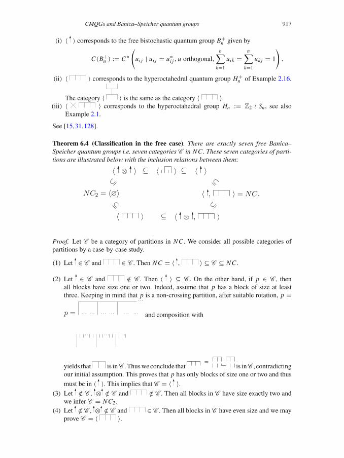
CMQGs and Banica–Speicher quantum groups 917
(i) 〈 〉 corresponds to the free bistochastic quantum group B+n given by
C(B+n ) := C∗
(ui j | ui j = u∗
i j , u orthogonal,n∑
k=1
uik =n∑
k=1
ukj = 1
).
(ii) 〈 〉 corresponds to the hyperoctahedral quantum group H+n of Example 2.16.
The category 〈 〉 is the same as the category 〈 〉.(iii) 〈 〉 corresponds to the hyperoctahedral group Hn := Z2 Sn , see also
Example 2.1.
See [15,31,128].
Theorem 6.4 (Classification in the free case). There are exactly seven free Banica–Speicher quantum groups i.e. seven categories C in NC. These seven categories of parti-tions are illustrated below with the inclusion relations between them:
NC2 = 〈∅〉
〈 ⊗ 〉 〈 〉 〈 〉
〈 , 〉 = NC.
〈 〉 〈 ⊗ , 〉
⊆⊆ ⊆
⊆
⊆⊆
⊆
Proof. Let C be a category of partitions in NC . We consider all possible categories ofpartitions by a case-by-case study.
(1) Let ∈ C and ∈ C . Then NC = 〈 , 〉 ⊆ C ⊆ NC .
(2) Let ∈ C and /∈ C . Then 〈 〉 ⊆ C . On the other hand, if p ∈ C , thenall blocks have size one or two. Indeed, assume that p has a block of size at leastthree. Keeping in mind that p is a non-crossing partition, after suitable rotation, p =
p = · · · · · · · · · · · · · · ·
· · ·
· · · and composition with
· · · · · · · · ·
yields that is inC . Thuswe conclude that=
is inC , contradictingour initial assumption. This proves that p has only blocks of size one or two and thus
must be in 〈 〉. This implies that C = 〈 〉.(3) Let /∈ C , ⊗ /∈ C and /∈ C . Then all blocks in C have size exactly two and
we infer C = NC2.(4) Let /∈ C , ⊗ /∈ C and ∈ C . Then all blocks in C have even size and we may
prove C = 〈 〉.

918 Moritz Weber
(5)–(7) Continue case study.
See [31,128]. �
Remark 6.5 (Dimensions issue). In principle, different categories will yield differentCMQGs, in the following sense:Given categoriesC1 �= C2, therewill be no *-isomorphismbetween their corresponding C∗-algebras mapping generators ui j to generators ui j . How-ever, for smaller values of n, some of the categories may yield the same quantum group.
Theorem 6.6 (Classification in the group case). There are exactly six Banica–Speichergroups, i.e. six categories with ∈ C .
(1) 〈 〉 (On).
(2) 〈 , 〉 (Bn)
(3) 〈 , ⊗ 〉 (Bn × Z2).(4) 〈 , 〉 (Hn)
(5) 〈 , , 〉 (Sn).
(6) 〈 , ⊗ , 〉 (Sn × Z2)
(Note that .)
Proof. As C0 := C ∩ NC ⊆ NC is a category, the previous theorem gives us all possibil-ities for C0. Clearly 〈C0, 〉 is contained in C . For the reverse inclusion, we note that thecrossing partition can be used to transform a partition with crossings to a non-crossingpartition. Thus C = 〈C0, 〉. See [31,128]. �
Theorem 6.7 (Classification in the half-liberated case). We may list all half-liberatedBanica–Speicher quantum groups, i.e. quantum groups whose category of partitions C
contains but not .
(1) 〈 〉 corresponds to O∗n given by
C(O∗n ) := C∗(ui j |ui j = u∗
i j , u orthogonal,
abc = bca where a = ui j , b = ukl , c = u pq).
We have On ⊆ O∗n ⊆ O+
n .
(2) 〈 , ⊗ 〉.(3) 〈 , 〉.(4) 〈 , , hs〉, s ≥ 3, where hs is the two block partition in P(0, 2s) such that all
odd points form one block while all even points form a second block.
See [128].
DEFINITION 6.8 (Hyperoctahedral case)
A category C ⊆ P is said to be hyperoctahedral if is in C , and ⊗ is not in C .
Theorem 6.9 (Classification in the non-hyperoctahedral case). There are exactly 13non-hyperoctahedral categories.

CMQGs and Banica–Speicher quantum groups 919
Proof.
(1) Let C ⊂ NC . By Theorem 6.4, we know that there are six non-hyperoctahedralcategories (only 〈 〉 is hyperoctahedral).
(2) Let C �⊂ NC and ∈ C . By Theorem 6.6, we know that there are five non-hyperoctahedral categories (only 〈 , 〉 is hyperoctahedral).
(3) Let C �⊂ NC and /∈ C . We may prove that we are in the situation /∈ C and
∈ C , thus by Theorem 6.7, there are two more non-hyperoctahedral categories.
See [128]. �
Theorem 6.10 (Classification in the hyperoctahedral case). If C is a category of par-titions in the hyperoctahedral case, then
(a) Either we are in the first case: C = 〈πk〉 for some k ∈ N or C = 〈πl , l ∈ N〉, whereπk ∈ P(0, 4k) is the partition given by k blocks each on four points arranged as
πk = a1a2 . . . akak . . . a2a1a1a2 . . . akak . . . a2a1,
(b) or we are in the second case: For n ∈ N, the CMQG G associated to C is given bythe semi direct product
C(G) ∼= C∗(�) ⊗ C(Sn),
ui j ↔ ugi vi j ,
where � is a quotient group of Z∗n2 with generators g1, . . . , gn and vi j are the gener-
ators of C(Sn).
Proof. Note that we may view partitions in P(0, n) as words of the length n, where blocksare represented by equal letters, thus corresponds to the word aaaa for instance,
whereas ⊗ is written as the word ab. If C is a category in the hyperoctahedral casecontaining the partition
aabaab ∈ P(0, 6),
we are in Case (b); otherwise we are in Case (a).
Case (a). If aabaab is not in C , we may infer that all partitions in C must obey some ‘pairnesting rule’; a typical partition looks like
abccbddaaeebba.
We may show that all such partitions may be constructed using the partitions πk and thecategory operations. See [103].Case (b). If aabaab is in C , we may restrict our attention to words (aka partitions) suchthat neighbouring letters are different – put differently, if a word contains two neighbouringequal letters, we may remove them (obtaining a word inC fromwhich we may reconstructour original word). This resembles words in Z
∗∞2 .
We thus define a subset F(C ) ⊂ Z∗∞2 consisting of all possible ways to represent a
partition in C as a word in the generators of Z∗∞2 . Then, F(C ) is

920 Moritz Weber
• a subgroup of Z∗∞2 (using the tensor product of partitions for the product of group
elements and the involution of partitions for the inversion of group elements),• normal (using the pair partition and the partition aabaab together with the composi-tion),
• invariant under certain endomorphisms of Z∗∞2 .
Conversely, to every such normal subgroup of Z∗∞2 , we obtain a hyperoctahedral category
of partitions in Case (b). We then take the quotient of Z∗n2 by the restriction F(C ) to n
letters in order to obtain �.See [101,102]. �
COROLLARY 6.11 (The classification of Banica–Speicher quantum groups is complete)
The classification of Banica–Speicher quantum groups is complete. Moreover, Theo-rem 6.10(b) shows that the world of Banica–Speicher quantum groups is very rich: Toevery variety of a group, we may associate a quotient group � of Z
∗∞2 in order to obtain a
Banica–Speicher quantum group in the sense of Theorem 6.10(b). Since there are uncount-ably many varieties of groups, the same holds true for the class of Banica–Speicher quan-tum groups.
7. Applications and use of Banica–Speicher quantum groups, state-of-the-art,open problems
7.1 Use of Banica–Speicher quantum groups for CQGs
Banica–Speicher quantum groups give rise to many new examples of CMQGs in thespirit of ‘liberation’ (i.e. omitting f g = g f for the function algebras, see Remark 2.18).They provide a whole class of quantum subgroups of O+
n and are thus a big step in thedirection of understanding all kinds of quantum rotations. Note that the machinery ofBanica–Speicher quantum groups has recently been extended to unitary Banica–Speicherquantum subgroups, i.e. we may now cover even quantum subgroups of U+
n , see [110].The class of Banica–Speicher quantum groups may be understood by combinatorial
means. In fact, the general philosophy is: ‘Everything about Banica–Speicher quantumgroups should be visible in terms of partitions.’ This has been proven successful, forinstance, regarding the Haar measure (‘Weingarten calculus’) [18] or the representationtheory (‘fusion rules’) [73]. Thus, understanding Banica–Speicher quantum groups viatheir combinatorics might help to get a better understanding for general CMQGs. Theresult of Theorem 6.10(b) is a first example of a structure theorem which was discoveredby studying the combinatorics of Banica–Speicher quantum groups first [101], but couldthen be extended also to non-Banica–Speicher quantum groups in a very general way[102]. One of the strategies to produce new results about CMQGs using Banica–Speicherquantum groups is the following:
• Take any result that holds for Sn, On or Un .• Make it ‘quantum’ by proving an analog for S+
n , O+n or U+
n .• Generalize it to Banica–Speicher quantum groups, ideally by finding a uniform proof(possibly using partitions).
• Generalize it to CMQGs.

CMQGs and Banica–Speicher quantum groups 921
7.2 Use of Banica–Speicher quantum groups for free probability
Free probability [99,118] profits from Banica–Speicher quantum groups in many ways.Firstly, we can do free probability on Banica–Speicher quantum groups. Indeed, anyCMQG comes as a C∗-algebra A with a (Haar) state h – thus, we have a noncommutativeprobability space and we may ask for the noncommutative distributions of the elementsui j , for instance, the ‘laws of characters’. This is doable for Banica–Speicher quantumgroups, as the Haar state is well-understood here [18]. It turns out, that the law of
∑i uii is
a semicircle in the case of O+n (which is in away the ‘Gauß distribution in free probability’)
and a free Poisson distribution in the case of S+n .
Secondly, Banica–Speicher quantum groups provide distributional symmetries for freeprobability in a de Finetti sense. Recall the classical de Finetti theorem:If (xn)n∈N is a sequence of classical, real random variables, then (xn)n∈N is independent
(over the tail σ -algebra) and identically distributed if and only if the distribution of (xn)n∈Nis invariant under the actions of Sn for all n ∈ N.
A free version of this theorem holds true [85]:If (xn)n∈N is a sequence of noncommutative, self-adjoint randomvariables, then (xn)n∈N
is free (over the tail von Neumann algebra) and identically distributed if and only if thedistribution of (xn)n∈N is invariant under the actions of S+
n for all n ∈ N.Refinements of this de Finetti theorem to other Banica–Speicher quantum groups have
been proven [24], see also §7.4.
7.3 Use of Banica–Speicher quantum groups for von Neumann algebras
As any CQG comes with a Haar state, we may perform the GNS construction and we maythus associate a vonNeumann algebra to aCQG.These ‘quantumgroupvonNeumann alge-bras’ are an own class of examples of vonNeumann algebras, besides thewell-knowngroupvon Neumann algebras. Those associated to O+
n share many properties with the famousfree group factors LFm ; however, they are not isomorphic to the free group factors [49].Amongst the properties for the von Neumann algebraic side of O+
n and U+n , we know
• their reduced C∗-algebras are non-nuclear, exact, simple and have the metric approx-imation property. They are K -amenable and their K -theory is
K0(C(O+n )) = Z, K1(C(O+
n )) = Z, K0(C(U+n )) = Z, K1(C(U+
n )) = Z2.
• the von Neumann algebras associated to them are strongly solid, non-injective, full,prime I I1 factors having the Haagerup approximation property and no Cartan subal-gebra.
• moreover, O+n and U+
n are weakly amenable and have the Akemann-Ostrand propertyas well as the property of rapid decay.
See [130] for an overview on the operator algebraic properties of Banica-Speicher quantumgroups, see also Section 7.4.
7.4 Overview on the literature on Banica–Speicher quantum groups and related work
The literature on Banica–Speicher quantum groups (also called easy quantum groups)is constantly growing. The official starting point was the initial article by Banica andSpeicher in 2009 [31]. However, there are many articles predating and preparing the theory

922 Moritz Weber
of Banica–Speicher quantum groups. They mainly deal with the quantum groups O+n , U+
nand S+
n and even nowadays when being interested in Banica–Speicher quantum groupsone should certainly consider the literature on these three special quantum groups as an‘extended literature on Banica–Speicher quantum groups’.In the sequel, we try to give a commented and complete list of the literature on Banica–
Speicher quantum groups and a commented but certainly incomplete list of the literatureon O+
n , U+n and S+
n . Note that our comments on the articles only highlight some aspectsand never present a full summary of the contents repsectively.
7.4.1 The roots within Woronowicz’s framework.
• [132,135]: Introduction of CMQGs.• [134]: Tannaka–Krein theorem for CMQGs, enabling a category approach to CMQGsand thus building the basis of the Banica–Speicher quantum group machine. See also[96] for a recent approach to Tannaka–Krein for CMQGs.
7.4.2 Predating work leading to Banica–Speicher quantum groups.
• [122]: Introduction of O+n , U+
n . See also [115] for their deformed versions.• [2,3]: Representation theory of O+
n and U+n .
• [124]: Introduction of S+n .
• [4]: Representation theory of S+n .
• [37]: Definition of H+n .
• [1,15,32]: Representation theory of H+n and related quantum groups.
• [18,19]: Computation of theHaar state of O+n , U+
n and S+n using partitions (Weingarten
calculus).• [85]: De Finetti theorems for S+
n . See also [58] for de Finetti theorems for O+n and
U+n and [57,59,61] for more on distributional quantum symmetries and further links
to free probability.
7.4.3Predating work on a diagrammatic calculus. Thediagrammatic calculus has diverseroots and appears in many disguises at many places in mathematics. We can only approx-imate the question of how partitions and CMQGs got combined at some point. However,it was mainly Banica who – over the time and in several articles, partially with coauthors– in the end manifested partitions and a diagrammatic calculus as an indispensable tool inthe theory of CMQGs.
• [50]: Using pair partitions (allowing crossings) in order to study the representationtheory of On .
• [131]: A similar calculus is used when computing integrals on groups with respect tothe Haar measure, today known as the Weingarten calculus. See, for instance, the workof Collins [56] for modern approaches.
• [83]: Diagrammatic approach to the Jones polynomial; pushed further by Bisch andJones [42] in 1997 in order to understand Fuss–Catalan algebras and Temperly–Liebalgebras.
• [134]: A diagrammatic calculus resembling the one in categories of partitions showsup throughout the investigation of quantum SU (n).

CMQGs and Banica–Speicher quantum groups 923
• [105]: Combinatorial approach to free probability theory using partitions; linking it toCMQGs in joint work with Köstler in 2009 [85]; see also [60,61] for further links tofree probability.
• [3,5,15,18,32]: Using partitions at several places when dealing with CMQGs, finallyleading to the theory of Banica-Speicher quantum groups.
7.4.4 Literature on Banica–Speicher quantum groups.
• [31]: Introduction of Banica–Speicher quantum groups (under the name ‘easy quantumgroups’); partial classification in the free case.
• [22]: Definition of the series H (s)n and H [s]
n as Banica–Speicher quantumgroups; partialclassification of non-hyperoctahedral Banica–Speicher quantum groups; computationof several laws of characters.
• [23]: Stochastic aspects of Banica–Speicher quantum groups.• [24]: Uniform de Finetti theorems for some Banica–Speicher quantum groups such as
S+n , O+
n , H+n and B+
n .• [100]: Isomorphism B+
n∼= O+
n−1 and others; fusion rules.• [30]: Quantum homogeneous spaces in certain Banica–Speicher quantum groups aris-ing as rectangular parts of the fundamental unitary (for instance as the first k lines).
• [128]: Complete classification in the free case, the non-hyperoctahedral case and thehalf-liberated case.
• [73]: Uniform fusion rules theorem for Banica–Speicher quantum groups; laterextended by Freslon in [68].
• [101–103]: Complete classification of all Banica–Speicher quantum groups (in partic-ular, in the hyperoctahedral case).
• [130]: Chapter on Banica–Speicher quantum groups in lecture notes on free probabilitytheory [118].
• [109,110]: Introduction of unitary Banica–Speicher quantum groups; complete clas-sification in the free case.
• [75]: Fixed point algebras for Banica–Speicher quantum groups.• [97]: Computation of theMartin boundary of the semi-direct product Banica–Speicherquantum groups (hyperoctahedral case).
7.4.5 Generalizations of Banica–Speicher quantum groups.
• [29]: Two-parameter versions of O+n , S+
n and other CMQGs; leading to Banica’s [11]definition of super-easy quantum groups in 2017.
• [69]: Group elements decorating points of partitions; see also [70].• [51]: Banica–Speicher quantum groups associated to three-dimensional partitions.
7.4.6 Further related work on O+n , U+
n and S+n (incomplete list). Again, let us empha-
size that the following list is composed and ordered from a subjective point of view (infact, the order is vaguely regarding subject matter, but it is not optimized). Many resultsabout O+
n , U+n and S+
n are hidden in further articles, possibly just as side remarks. More-over, we decided to refrain from including all results about the deformations of O+
n andU+
n (as defined in [115]), because sometimes the undeformed cases behave special andare excluded though, and also, as Woronowicz’s SUq(2) can be seen as a deformation of

924 Moritz Weber
O+2 (see Example 2.15), this would then exceed our capacities for assembling a list of
literature. So, we more or less restricted our attention to the exposition of work directlyrelated to O+
n , U+n and S+
n , and we sincerely apologize for any gap in our list – and thereare certainly many! – as well as for the quite restricted (and again, incomplete) expo-sition of the contents of the respective articles. In particular, many articles by Banicaand coauthors are missing, one could almost add his whole list of publications to the listbelow.
• [16]: Survey on S+n .
• [17]: There are no intermediate quantum groups between On and O∗n .
• [33,39]: On O∗n and other half-liberated quantum groups.
• [21]: Spectral measure of ui j ∈ C(O+n ).
• [26]: O+n as the quantum isometry group (in Goswami’s sense) of the free sphere,
within the framework of Connes’s noncommutative geometry; see also [8,9,76,106]for related work.
• [112]: The factor associated to O+n is solid, prime and has the Akemann–Ostrand
property; the reduced C∗-algebra associated to O+n is exact.
• [43–46]: Properties of von Neumann algebras associated to O+n , U+
n and S+n and oth-
ers, such as the Haagerup approximation property (HAP), the metric approximationproperty, Haagerup inequalities and others.
• [62,67]: CCAP for O+n , weak amenability for O+
n and U+n .
• [79,80]: The von Neumann algebra associated to O+n has no Cartan subalgebra.
• [91]: HAP for H+n and others.
• [34]: Kirchberg’s factorization property for O+n and U+
n .• [71]: MASA on O+
n .• [48]: Connes Embedding Property (CEP) for O+
n and U+n .
• [49]: The factors associated to O+n are not isomorphic to the free group factors.
• [47]: O+n and entanglement in quantum information theory.
• [119,120]: K -theory of O+n and S+
n , see also [117] for more on this and the case U+n .
• [72,78,93]: Other de Finetti theorems related to S+n (Boolean, monotone and bi-free
independence).• [41,89,116]: Computation of 2-Betti numbers of O+
n and U+n .
• [38]: Hochschild cohomology on S+n ; see also [40].
• [125]: S+n and O+
n are simple; see also [53,126,127].• [54]: U+
n is residually finite dimensional.• [81]: Hopf images in S+
4 and automorphisms of S+4 .
• [20]: Models for S+n , i.e. matrices in Mk(C(X)) for some compact space X providing
representations of C(S+n ); see also [10,13,25,27] for more on this subject.
• [37]: Introduction of free wreath products of CMQGs; see also [64,70,90,92,107,121]for more on this subject.
• [6,36]: Quantum automorphisms of graphs; see also [12,14,37,52,74,104,106] formore on this subject.
• [28]: Links between S+n and the Hadamard conjecture; see also [7].
• [55]: Stochastic processes on O+n ; see also [65,66] for more on this subject.

CMQGs and Banica–Speicher quantum groups 925
7.5 Open problems
Although the theory of Banica–Speicher quantum groups is already quite well studied,there are still many open problems and questions. We only list a few of them. Others – andmore technical ones – may be found in various articles of §7.4.4.
7.5.1 Intermediate and non-Banica–Speicher quantum groups. From [17], we knowthat there is no quantum group G such that On � G � O∗
n . How about those withO∗
n � G � O+n ?
In general, we know, that the only Banica–Speicher quantum group sitting strictlybetween On and O+
n is the half-liberated quantum group O∗n , but we do not know whether
there is any other (non-Banica–Speicher) quantum group G in between On and O+n . More-
over, it is unkown whether there is a quantum group G sitting in between Sn and S+n , if so
is Sn � G � S+n ?
It is easy to show, that there cannot be a Banica–Speicher QG, but we do not knowwhether there is any non–Banica–Speicher quantum group in that strip.More generally, wecan ask for examples of non-Banica–Speicher quantum groups G such that Sn ⊂ G ⊂ U+
n .Almost nothing is known about this question, see [102] for some indirect examples.
7.5.2 Deformations of Banica–Speicher quantum groups. The quantum groups O+n
and U+n admit deformations to non-Kac quantum groups O+(Q) and U+(Q), see Exam-
ples 2.13, and 2.14, and [115]. It is not so difficult to see that the intertwiner spaces ofO+(Q)may again be described by noncrossing pair partitions, just like in the case Q = 1n ,which is O+
n . However, it is absolutely unclear how to define Q-deformations of Banica–Speicher quantum groups, i.e. how to define analogs G(Q) ⊂ U+(Q) of Banica–Speicherquantum groups G ⊂ U+
n such that their intertwiner spaces are again given by the samecategory of partitions. In other words, given a category of partitions C , the assignmentp → Tp (see Definition 5.3) allows us to associate a concrete W ∗-category to C , seeProposition 5.8. The crucial fact is that the operations on the partitions, like tensor prod-uct, composition and involution, behave nicely with respect to the assignment p → Tp, seeProposition 5.5. Wemay therefore ask: Is there a way to deform the phase functor p → Tp
such that suitable (maybe slightly weaker) analogs of Propositions 5.5 and 5.8 hold? Canwe then associate ‘deformed Banica-Speicher’ quantum groups G(Q) ⊂ U+(Q) to cate-gories of partitions?
7.5.3 Classification in the unitary case. The classification of all orthogonal Banica–Speicher quantum groups is settled, see Corollary 6.11 and [103]. In the unitary casehowever, the situation is quite the converse:Almost nothing is known about unitaryBanica–Speicher quantum groups. The task is to classify all categories of colored partitions, see[109]; they correspond to Banica–Speicher quantum groups G such that
Sn ⊂ G ⊂ U+n .
In [109], we classified all categories of noncrossing colored partitions, i.e. the case
S+n ⊂ G ⊂ U+
n .
Moreover, we found all classical Banica–Speicher groups
Sn ⊂ G ⊂ Un .

926 Moritz Weber
It is natural to ask for the case
Un ⊂ G ⊂ U+n .
Further natural questions about partial classifications are (derived from the observationsin the orthogonal case): Which are all half-liberated unitary Banica–Speicher quantumgroups? Which are all categories/quantum groups in the non-hyperoctahedral case? Dowe have a unitary semi-direct product construction as in [102]? See also [110] for morequestions. Note that in the situation of generalizations of Banica–Speicher quantum groups(see §7.4.5) even further classification problems await their completion. The flavour ofthese problems is by large means of combinatorial nature.
7.5.4 Laws of characters. One important characteristics of a CMQG is its law ofcharacters. More precisely, let (A, u) be a CMQG and let h be its Haar state. We putχ :=∑i uii ∈ A. The law of (A, u) is by definition the collection of all moments:
h(χk), k ∈ N.
One can show that h(χk) coincides with
dim Mor(u⊗k, u⊗k).
The law of a CMQG thus contains important information about the intertwiner spaces aswell as about the Haar state. If (A, u) is a Banica–Speicher quantum group and if the mapsTp for p ∈ C are linearly independent (for instance, when C ⊂ NC), the computation ofthe law of characters amounts to a combinatorial counting problem:
|C (k, k)| = ?
In order to express the law of a quantum group, the language of free probability theory isappropriate (see also §7.2) – we need to find a noncommutative random variable x in anoncommutative probability space (B, ϕ) such that
ϕ(xk) = h(χk), for all k ∈ N
holds, i.e. the noncommutative distributions of x and χ coincide. We then say that the lawof the CMQG (A, u) is the law of x ∈ (B, ϕ). Examples of such laws are the semicirclelaw (somehow the ‘Gaussian law of free probability’) for O+
n or the free Poisson law (alsocalledMarchenko–Pastur law) for S+
n , in analogywith the classicial situation: Gaussian forOn and Poisson for Sn . See [128] for more on laws of characters for CMQG and Banica–Speicher quantum groups and [129] for more on noncommutative probability spaces andnoncommutative distributions.There are many Banica–Speicher quantum groups for which we do not know the law
of characters including those from the semi-direct product construction [102] as well asthose arising from the categories 〈πk〉 in [103].
7.5.5 Uniform proofs for Banica–Speicher quantum groups. One of the striking featuresof Banica–Speicher quantum groups is that they are in a way a class of ‘combinatorialquantum groups’ in the sense that most of the properties of a Banica–Speicher quantumgroup should be hidden in its combinatorial data – the philosophy is that we should beable to read the properties of a Banica–Speicher quantum group from its category ofpartitions. As a consequence, for any property that holds for all Banica–Speicher quantumgroups (ormaybe for a large subclass) we should find a uniform proof in terms of partitions.
CMQGs and Banica–Speicher quantum groups 927
Examples for such a strategy are the uniform de Finetti proof [24], theWeingarten calculusfor Banica–Speicher quantum groups [18], the fusion rules [73] or the semi-direct productquantum groups [101]. A generic open problem is now to find uniform proofs for propertiesof Banica–Speicher quantum groups. Ideally, this would lead to some general insight forCMQGs in the sense that certain properties of CMQGs may be derived directly from theirintertwiner spaces, see for instance [102]. See also §7.1.
Now, many of the properties listed in §7.4.6 are known only for O+n , U+
n and/or S+n .
For each of these properties, we may now ask:
(1) Is it true for all three quantum groups O+n , U+
n and S+n ? Is it true for all free Banica–
Speicher quantum groups S+n ⊂ G ⊂ U+
n ? Is it true for all Banica–Speicher quantumgroups?
(2) Is there a uniform proof of this phenomenon? Can we express the property by meansof partitions, i.e. do we have a theorem/proof like:
If C is a category of partitions with property X , then the associated Banica–Speicher quantum group has the property Y .
(3) Can we generalize the uniform proof in a way such that it holds for a large class ofCMQGs, even non-Banica–Speicher ones?
One property for which a uniform proof seems possible is the Haagerup property (HAP).
7.5.6 A diagrammatical calculus for partially commutative quantum groups. It is anatural desire to extend the powerfulmachine of indexing intertwiners by partitions to otherCMQGs. One class for which first ideas are around are the partially commutative quantumgroups Oε
n , Sεn , etc. as introduced in [106]. Here, ε ∈ Mn({0, 1}) is a symmetric matrix
with εi i = 0 and the quantum groups Gε arise from imposing some partial commutationrelations on the generators ui j ∈ C(Gε). In the extreme case εi j = 1 for all i �= j , weobtain Oε
n = On and Sεn = Sn , whereas the other extreme case εi j = 0 for all i, j yields
Oεn = O+
n and Sεn = S+
n . Moreover, ε may be seen as the adjacency matrix of a finite,undirected graph �ε without loops, and Sε
n is exactly the quantum automorphism group of�ε as defined by Bichon [36].Hence, understanding the intertwiner spaces of these ε-quantum groups would help to
understand the intertwiner spaces of quantum automorphism groups of graphs, amongstothers – besides understanding this new class of CMQGs itself, formed by the ε-quantumgroups. Since the extreme cases include Banica–Speicher quantum groups, it seems plau-sible that a diagrammatic calculus based on partitions (with some extensions and possiblyrestricting tomatrices ε with certain technical conditions) shouldwork for the ε-intertwinerspaces as well, see [106] for first attempts in this direction. However, for the moment, basi-cally nothing is known about the intertwiner spaces of these quantum groups.
7.5.7 Further open problems. Further open problems may be found in the various arti-cles mentioned in §7.4.4 as well as in §7.4.6. In the following list, we will only very brieflylink to some of them.
• [7]: Many open problems, questions and conjectures regarding the links between S+n
and the Hadamard conjecture.• [24]: Find de Finetti theorems for all Banica–Speicher quantum groups (linked to thequestion of finding the laws of characters).

928 Moritz Weber
• [30]: How to fill up a rectangular matrix (ui j )1≤i≤n,1≤ j≤k to a square matrix(ui j )1≤i, j≤n of a Banica–Speicher quantum group (A, u)? (In the language of thepaper: When is the map in [30, Prop. 5.4] proper for general k, n?)
• [126]: Wang’s program of classifying simple compact quantum groups; see in partic-ular, [126, Sect. 6].
• [76]: How can Banica–Speicher quantum groups be seen as the quantum symmetriesof some quantum spaces, in particular: as quantum isometry groups in Goswami’sframework? See, in particular, [76, Sect. 10].
Acknowledgements
The authorwould like to thankV. S. Sunder for his invitation to IMSc, Chennai, for his greathospitality and his vision and support to get these lecture notes produced. He would like towish him all the best for his retirement, in deepest admiration for all of his mathematicalachievements. Furthermore, he thanks Soumya for all his great work regarding the contentsand the design of these notes and for providing all the figures. The author thanks PierreFima and Issan Patri for their various and valuable critical remarks throughout the lecturesat IMSc. He also thanks Felix Leid and Simon Schmidt for improvements regarding theexposition in the chapter on Tannaka–Krein theory. The author was partially supported bythe ERC Advanced Grant NCDFP, held by Roland Speicher.
References
[1] Banica T, Belinschi S T, Capitaine M and Collins B, Free Bessel laws, Canad. J. Math. 63(1)(2011) 3–37
[2] Banica T, Théorie des représentations du groupe quantique compact libre O(n), C. R. Acad.Sci. Paris Sér. I Math. 322(3) (1996) 241–244
[3] Banica T, Le groupe quantique compact libre U(n), Comm. Math. Phys. 190(1) (1997) 143–172
[4] Banica T, Symmetries of a generic coaction, Math. Ann. 314(4) (1999) 763–780.[5] Banica T, Quantum groups and Fuss-Catalan algebras, Comm. Math. Phys., 226(1) (2002)
221–232[6] Banica T, Quantum automorphism groups of homogeneous graphs, J. Funct. Anal. 224(2)
(2005) 243–280[7] Banica T, Quantum permutations, Hadamard matrices, and the search for matrix models, in:
Operator algebras and quantum groups, volume 98 of Banach Center Publ. (2012) (PolishAcad. Sci. Inst. Math., Warsaw) pp. 11–42
[8] Banica T, Liberations and twists of real and complex spheres, J. Geom. Phys. 96 (2015) 1–25[9] Banica T, Quantum isometries of noncommutative polygonal spheres, Münster J. Math. 8(1)
(2015) 253–284[10] Banica T, Quantum groups from stationary matrix models, Colloq. Math. 148(2) (2017) 247–
267[11] Banica T, Super-easy quantum groups: definition and examples, arXiv:1706.00152 (2017)[12] Banica T and Bichon J, Quantum automorphism groups of vertex-transitive graphs of order
≤11, J. Algebraic Combin. 26(1) (2007) 83–105[13] Banica T and Bichon J, Random walk questions for linear quantum groups, Int. Math. Res.
Not. IMRN 24 (2015) 13406–13436[14] Banica T, Bichon J and Chenevier G, Graphs having no quantum symmetry, Ann. Inst. Fourier
(2007) 955–971

CMQGs and Banica–Speicher quantum groups 929
[15] Banica T, Bichon J and Collins B, The hyperoctahedral quantum group, J. Ramanujan Math.Soc. 22(4) (2007) 345–384
[16] Banica T,Bichon J andCollinsB,Quantumpermutation groups: a survey, in:Noncommutativeharmonic analysis with applications to probability, volume 78 of Banach Center Publ. (2007)(Polish Acad. Sci. Inst. Math., Warsaw) pp. 13–34
[17] Banica T, Bichon J, Collins B and Curran S, A maximality result for orthogonal quantumgroups, Comm. Algebra 41(2) (2013) 656–665
[18] Banica T and Collins B, Integration over compact quantum groups. Publ. Res. Inst. Math. Sci.43(2) (2007) 277–302
[19] Banica T and Collins B, Integration over quantum permutation groups, J. Funct. Anal. 242(2)(2007) 641–657
[20] Banica T and Collins B, Integration over the Pauli quantum group, J. Geom. Phys. 58(8)(2008) 942–961
[21] Banica T, Collins B and Zinn-Justin P, Spectral analysis of the free orthogonal matrix, Int.Math. Res. Not. IMRN 17 (2009) 3286–3309
[22] Banica T, Curran S and Speicher R, Classification results for easy quantum groups, Pacific J.Math. 247(1) (2010) 1–26
[23] Banica T, Curran S and Speicher R, Stochastic aspects of easy quantum groups, Probab.Theory Related Fields 149(3–4) (2011) 435–462
[24] Banica T, Curran S and Speicher R, De Finetti theorems for easy quantum groups, Ann.Probab. 40(1) (2012) 401–435
[25] Banica T and Freslon A, Modelling questions for quantum permutations, arXiv:1704.00290(2017)
[26] Banica T and Goswami D, Quantum isometries and noncommutative spheres, Comm. Math.Phys. 298(2) (2010) 343–356
[27] Banica T and Nechita I, Flat matrix models for quantum permutation groups, Adv. in Appl.Math. 83 (2017) 24–46
[28] Banica T and Nicoara R, Quantum groups and Hadamard matrices, Pan. Amer. Math. J. 17(1)(2007) 1–24
[29] Banica T and Skalski A, Two-parameter families of quantum symmetry groups, J. Funct.Anal. 260(11) (2011) 3252–3282
[30] Banica T, Skalski A and Sołtan P, Noncommutative homogeneous spaces: the matrix case, J.Geom. Phys. 62(6) (2012) 1451–1466
[31] Banica T and Speicher R, Liberation of orthogonal Lie groupsm, Adv. Math. 222(4) (2009)1461–1501
[32] Banica T and Vergnioux R, Fusion rules for quantum reflection groups, J. Noncommut. Geom.3(3) (2009) 327–359
[33] Banica T andVergniouxR, Invariants of the half-liberated orthogonal group,Ann. Inst. Fourier(Grenoble) 60(6) (2010) 2137–2164
[34] Bhattacharya A and Wang S, Kirchberg’s factorization property for discrete quantum groups,Bull. Lond. Math. Soc. 48(5) (2016) 866–876
[35] Bhowmick J and Goswami D, Quantum isometry groups: examples and computations,Comm.Math. Phys. 285(2) (2009) 421–444
[36] Bichon J, Quantum automorphism groups of finite graphs, Proc. Amer. Math. Soc. 131(3)(2003) 665–673
[37] Bichon J, Free wreath product by the quantum permutation group, Algebr. Represent. Theory,7(4) (2004) 343–362
[38] Bichon J, Gerstenhaber–Schack and Hochschild cohomologies of Hopf algebras, Doc. Math.21 (2016) 955–986
[39] Bichon J andDubois-VioletteM,Half-commutative orthogonalHopf algebras,Pacific J. Math.263(1) (2013) 13–28
[40] Bichon J, Franz U and Gerhold M, Homological properties of quantum permutation algebras,arXiv:1704.00589 (2017)

930 Moritz Weber
[41] Bichon J, Kyed D and Raum S, Higher l2-Betti numbers of universal quantum groups,arXiv:1612.07706 (2016)
[42] Bisch D and Jones V, Algebras associated to intermediate subfactors, Invent. Math. 128(1)(1997) 89–157
[43] Brannan M, Approximation properties for free orthogonal and free unitary quantum groups,J. Reine Angew. Math. 672 (2012) 223–251
[44] Brannan M, Quantum symmetries and strong Haagerup inequalities, Comm. Math. Phys.311(1) (2012) 21–53
[45] Brannan M, Reduced operator algebras of trace-perserving quantum automorphism groups,Doc. Math. 18 (2013) 1349–1402
[46] Brannan M, Strong asymptotic freeness for free orthogonal quantum groups, Canad. Math.Bull. 57(4) (2014) 708–720
[47] Brannan M and Collins B, Highly entangled, non-random subspaces of tensor products fromquantum groups, arXiv:1612.09598 (2016)
[48] Brannan M, Collins B and Vergnioux R, The Connes embedding property for quantum groupvon Neumann algebras, Trans. Amer. Math. Soc. 369(6) (2017) 3799–3819
[49] BrannanM and Vergnioux R, Orthogonal free quantum group factors are strongly 1-bounded,arXiv:1703.08134 (2017)
[50] Brauer R, On algebras which are connected with the semisimple continuous groups, Ann.Math. (2) , 38(4) (1937) 857–872
[51] CébronGandWeberM,Quantumgroups based on spatial partitions, arXiv:1609.02321 (2016)[52] Chassaniol A, Quantum automorphism group of the lexicographic product of finite regular
graphs, J. Algebra (2016) 23–45[53] Chirvasitu A, Free unitary groups are (almost) simple, J. Math. Phys. 53(12) (2012) 123509,
7[54] Chirvasitu A, Residually finite quantum group algebras, J. Funct. Anal. 268(11) (2015) 3508–
3533[55] Cipriani F, Franz U and Kula A, Symmetries of Lévy processes on compact quantum groups,
their Markov semigroups and potential theory, J. Funct. Anal. 266(5) (2014) 2789–2844[56] Collins B and Sho M, Weingarten calculus via orthogonality relations: new applications,
arXiv:1701.04493 (2017)[57] Curran S, Quantum exchangeable sequences of algebras, Indiana Univ. Math. J. 58(3) (2009)
1097–1125[58] Curran S. Quantum rotatability, Trans. Amer. Math. Soc. 362(9) (2010) 4831–4851[59] Curran S, A characterization of freeness by invariance under quantum spreading, J. Reine
Angew. Math. 659 (2011) 43–65[60] Curran S and Speicher R, Asymptotic infinitesimal freeness with amalgamation for Haar
quantum unitary random matrices, Comm. Math. Phys. 301(3) (2011) 627–659[61] Curran S and Speicher R, Quantum invariant families of matrices in free probability, J. Funct.
Anal., 261(4) (2011) 897–933[62] De Commer K, Freslon A and Yamashita M, CCAP for universal discrete quantum groups,
Comm. Math. Phys. 331(2) (2014) 677–701. With an appendix by Stefaan Vaes[63] Enock M and Schwartz J-M, Kac algebras and duality of locally compact groups (1992)
(Berlin: Springer-Verlag), With a preface byAlainConnes,with a postface byAdrianOcneanu[64] Fima P and Pittau L, The free wreath product of a compact quantum group by a quantum
automorphism group, J. Funct. Anal. 271(7) (2016) 1996–2043[65] Franz U, Hong G, Lemeux F, Ulrich M and Zhang H, Hypercontractivity of heat semigroups
on free quantum groups, J. Operator Theory 77(1) (2017) 61–76[66] Franz U, Kula A and Skalski A, Lévy processes on quantum permutation groups, in: Noncom-
mutative analysis, operator theory and applications, volume 252 of Oper. Theory Adv. Appl.(2016) (Birkhäuser/Springer) [Cham] pp. 193–259
[67] Freslon A, Examples of weakly amenable discrete quantum groups, J. Funct. Anal. 265(9)(2013) 2164–2187

CMQGs and Banica–Speicher quantum groups 931
[68] Freslon A, Fusion (semi)rings arising from quantum groups, J. Algebra, 417 (2014) 161–197[69] Freslon A, On the partition approach to Schur–Weyl duality and free quantum groups, Trans-
formation groups (2016) 1–45[70] Freslon A and Skalski A, Wreath products of finite groups by quantum groups,
arXiv:1510.05238 (2015)[71] Freslon A and Vergnioux R, The radial MASA in free orthogonal quantum groups, J. Funct.
Anal. 271(10) (2016) 2776–2807[72] Freslon A and Weber M, On bi-free de Finetti theorems, Ann. Math. Blaise Pascal 23(1)
(2016) 21–51[73] Freslon A and Weber M, On the representation theory of partition (easy) quantum groups, J.
Reine Angew. Math. 720 (2016) 155–197[74] Fulton M, The quantum automorphism group and undirected trees. Ph.D. Thesis, Virginia
(2006)[75] Gabriel O and Weber M, Fixed point algebras for easy quantum groups. SIGMA Symmetry
Integrability Geom. Methods Appl. 12 Paper No. 097, 21 (2016)[76] Goswami D and Bhowmick J, Quantum isometry groups, Infosys Science Foundation Series,
Springer, New Delhi (2016), Infosys Science Foundation Series in Mathematical Sciences.[77] José M, Gracia-Bondí A, Várilly J C and Figueroa H, Elements of noncommutative geometry,
Birkhäuser Advanced Texts: Basler Lehrbücher, [Birkhäuser Advanced Texts: Basel Text-books], Birkhäuser Boston, Inc., Boston, MA (2001)
[78] Hayase T, De Finetti theorems for a Boolean analogue of easy quantum groups,arXiv:1507.05563 (2015)
[79] Isono Y, Examples of factors which have no Cartan subalgebras, Trans. Amer. Math. Soc.367(11) (2015) 7917–7937
[80] Isono Y, Cartan subalgebras of tensor products of free quantum group factors with arbitraryfactors, arXiv:1607.02847 (2016)
[81] Józiak P, Remark on Hopf images in quantum permutation groups S+n , arXiv:1611.09211
(2016)[82] Kassel C, Quantum groups, volume 155 of Graduate Texts in Mathematics (1995) (Springer-
Verlag, New York)[83] Kauffman L H, State models and the Jones polynomial, Topology 26(3) (1987) 395–407[84] Klimyk A and Schmüdgen K, Quantum groups and their representations, Texts and Mono-
graphs in Physics (1997) (Berlin: Springer-Verlag)[85] Köstler C and Speicher R, A noncommutative de Finetti theorem: invariance under quantum
permutations is equivalent to freeness with amalgamation, Comm. Math. Phys. 291(2) (2009)473–490
[86] Kustermans J and Tuset L, A survey of C∗-algebraic quantum groups, I, Irish Math. Soc. Bull.43 (1999) 8–63
[87] Kustermans J and Tuset L, A survey of C∗-algebraic quantum groups, II, Irish Math. Soc.Bull. 44 (2000) 6–54
[88] Kustermans J and Vaes S, Locally compact quantum groups in the von Neumann algebraicsetting, Math. Scand. 92(1) (2003) 68–92
[89] KyedD andRaumS,On the l2-Betti numbers of universal quantum groups, arXiv:1610.05474(2016)
[90] Lemeux F, The fusion rules of some free wreath product quantum groups and applications, J.Funct. Anal. 267(7) (2014) 2507–2550
[91] Lemeux F, Haagerup approximation property for quantum reflection groups, Proc. Amer.Math. Soc. 143(5) (2015) 2017–2031
[92] Lemeux F andTarrago P, Freewreath product quantumgroups: themonoidal category, approx-imation properties and free probability, J. Funct. Anal., 270(10) (2016) 3828–3883
[93] Liu W. Extended de Finetti theorems for boolean independence and monotone independence,arXiv:1505.02215 (2015)

932 Moritz Weber
[94] Lusztig G, Introduction to quantum groups, volume 110 of Progress in Mathematics (1993)(Boston, MA: Birkhäuser Boston Inc.)
[95] Maes A and Van Daele A, Notes on compact quantum groups, Nieuw Arch. Wisk. (4) 16(1–2)(1998) 73–112
[96] Malacarne S, Woronowicz’s Tannaka–Krein duality and free orthogonal quantum groups,arXiv:1602.04807 (2016)
[97] Malacarne S and Neshveyev S, Probabilistic boundaries of finite extensions of quantumgroups, arXiv:1704.04717 (2017)
[98] Neshveyev S and Tuset L, Compact quantum groups and their representation categories,volume 20 of Cours Spécialisés [Specialized Courses] (2013) (Paris: Société Mathématiquede France)
[99] Nica A and Speicher R, Lectures on the combinatorics of free probability, volume 335 ofLondonMathematical Society LectureNote Series (2006) (Cambridge: CambridgeUniversityPress)
[100] Raum S, Isomorphisms and fusion rules of orthogonal free quantum groups and their freecomplexifications, Proc. Amer. Math. Soc. 140(9) (2012) 3207–3218
[101] Raum S andWeber M, The combinatorics of an algebraic class of easy quantum groups, Infin.Dimens. Anal. Quantum Probab. Relat. Top. 17(3) (2014) 1450016, 17
[102] Raum S andWeber M, Easy quantum groups and quantum subgroups of a semi-direct productquantum group, J. Noncommut. Geom. 9(4) (2015) 1261–1293
[103] Raum S and Weber M, The full classification of orthogonal easy quantum groups, Comm.Math. Phys. 341(3) (2016) 751–779
[104] Schmidt S and Weber M, Quantum symmetries of graph C*-algebras, arXiv:1706.08833(2017)
[105] Speicher R, A new example of ‘independence’ and ‘white noise’, Probab. Theory RelatedFields 84(2) (1990) 141–159
[106] Speicher R and Weber M, Quantum groups with partial commutation relations,arXiv:1603.09192 (2016)
[107] Tarrago P and Wahl J, Free wreath product quantum groups and standard invariants of sub-factors, arXiv:1609.01931 (2016)
[108] Tarrago P and Weber M, Appendix, in: Unitary easy quantum groups: the free case and thegroup case, arXiv:1512.00195 (2015)
[109] Tarrago P and Weber M, The classification of tensor categories of two-colored noncrossingpartitions, arXiv:1509.00988 (2015)
[110] Tarrago P and Weber M. Unitary easy quantum groups: the free case and the group case, Int.Math. Res. Not. (2016)
[111] TimmermannT,An invitation to quantumgroups and duality, EMSTextbooks inMathematics,European Mathematical Society (EMS), Zürich, (2008) From Hopf algebras to multiplicativeunitaries and beyond
[112] Vaes S and Vergnioux R, The boundary of universal discrete quantum groups, exactness, andfactoriality, Duke Math. J. 140(1) (2007) 35–84
[113] Van Daele A, Dual pairs of Hopf ∗-algebras, Bull. London Math. Soc., 25(3) (1993) 209–230[114] VanDaele A, TheHaarmeasure on a compact quantum group,Proc. Amer. Math. Soc. 123(10)
(1995) 3125–3128[115] Van Daele A andWang S, Universal quantum groups, Internat. J. Math. 7(2) (1996) 255–263[116] Vergnioux R, Paths in quantum Cayley trees and L2-cohomology, Adv. Math. 229(5) (2012)
2686–2711[117] Vergnioux R and Voigt C, The K -theory of free quantum groups, Math. Ann. 357(1) (2013)
355–400[118] Voiculescu D-V, Stammeier N andWeber M, Free probability and operator algebras, Münster
Lecture Notes in Mathematics (2016) (Zürich: Eur. Math. Soc. (EMS))[119] Voigt C, TheBaum-Connes conjecture for free orthogonal quantumgroups,Adv. Math., 227(5)
(2011) 1873–1913

CMQGs and Banica–Speicher quantum groups 933
[120] Voigt C, On the structure of quantum automorphism groups, J. Reine Angew. Math. (2015)[121] Wahl J, A note on reduced and von Neumann algebraic free wreath products, Illinois J. Math.
59(3) (2015) 801–817[122] Wang S, Free products of compact quantum groups, Comm. Math. Phys. 167(3) (1995)
671–692[123] Wang S, Tensor products and crossed products of compact quantum groups, Proc. London
Math. Soc. (3), 71(3) (1995) 695–720[124] Wang S, Quantum symmetry groups of finite spaces, Comm. Math. Phys. 195(1) (1998)
195–211[125] Wang S, Simple compact quantum groups, I, J. Funct. Anal. 256(10) (2009) 3313–3341[126] Wang S, On the problem of classifying simple compact quantum groups, in: Operator algebras
and quantum groups, volume 98 of Banach Center Publ. (2012) (Warsaw: Polish Acad. Sci.Inst. Math.) pp. 433–453
[127] Wang S, Equivalent notions of normal quantum subgroups, compact quantum groups withproperties F , and other applications, J. Algebra 397 (2014) 515–534
[128] Weber M, On the classification of easy quantum groups, Adv. Math., 245 (2013) 500–533[129] Weber M, Basics in free probability, in: Free probability and operator algebras, Münster
Lectures in Mathematics (2016) (Zürich: European Mathematical Society (EMS))[130] Weber M, Easy quantum groups, in: Free probability and operator algebras, Münster Lectures
in Mathematics (2016) (Zürich: European Mathematical Society (EMS))[131] Weingarten D. Asymptotic behavior of group integrals in the limit of infinite rank, J. Mathe-
matical Phys. 19(5) (1978) 999–1001[132] Woronowicz S L, Compact matrix pseudogroups,Comm. Math. Phys. 111(4) (1987) 613–665[133] WoronowiczSL,TwistedSU(2) group.An example of a noncommutative differential calculus,
Publ. Res. Inst. Math. Sci. 23(1) (1987) 117–181[134] Woronowicz S L, Tannaka–Kreın duality for compact matrix pseudogroups, Twisted SU(N )
groups, Invent. Math. 93(1) (1988) 35–76[135] Woronowicz S L, A remark on compact matrix quantum groups, Lett. Math. Phys. 21(1)
(1991) 35–39[136] Woronowicz S L, Compact quantum groups, in: Symétries quantiques (Les Houches, 1995)
(1998) (Amsterdam: North-Holland) pp. 845–884
Communicating Editor: B V Rajarama Bhat