introduction to computational manifolds and applicationsjean/au11.pdf · introduction to...
TRANSCRIPT

Introduction to Computational Manifolds and Applications
Prof. Marcelo Ferreira Siqueira
Departmento de Informática e Matemática Aplicada Universidade Federal do Rio Grande do Norte
Natal, RN, Brazil
IMPA - Instituto de Matemática Pura e Aplicada, Rio de Janeiro, RJ, Brazil
Part 1 - Constructions

Parametric Pseudo-Manifolds
Computational Manifolds and Applications (CMA) - 2011, IMPA, Rio de Janeiro, RJ, Brazil 2
Transition Maps
We will now study some "candidates" for the g maps of our transition maps.
First, we will consider projective transformations in RP2.
Next, we will review some simple conformal maps.
Both maps above do not fulfill all requirements for the role of the g maps. But, if weallow a slight change in the geometry of the p-domains, simple conformal maps cando the job.

Parametric Pseudo-Manifolds
Computational Manifolds and Applications (CMA) - 2011, IMPA, Rio de Janeiro, RJ, Brazil 3
Projective Transformations
Our goal now is to define a projective transformation, T : RP2 → RP2, that mapsQuw
ontoQ.
Any basis with the above property is said to be associated with the projective frame(ai)1≤i≤n+2.
Recall that a family, (ai)1≤i≤n+2, of n + 2 points of the projective space RPn is aprojective frame (or basis) of RPn if there exists some basis (e1, . . . , en+1) of Rn+1 suchthat
ai = [ei]∼ , for 1 ≤ i ≤ n + 1
andan+2 = [en+2]∼ , where en+2 = e1 + · · · + en + en+1.

Parametric Pseudo-Manifolds
Computational Manifolds and Applications (CMA) - 2011, IMPA, Rio de Janeiro, RJ, Brazil 4
Projective Transformations
We can view each ai as a line in Rn+1 passing through the origin in the direction ofei.
For instance,e1 = (1, 0, . . . , 0, 0)e2 = (0, 1, . . . , 0, 0)
...en = (0, 0, . . . , 1, 0)
en+1 = (0, 0, . . . , 0, 1) ,
the canonical basis of Rn+1, together with the vector en+2 = e1 + · · · + en+1, defines aprojective frame, (a1, . . . , an+2), of RPn such that ai = [ei]∼, for every 1 ≤ i ≤ n + 2.

Parametric Pseudo-Manifolds
Computational Manifolds and Applications (CMA) - 2011, IMPA, Rio de Janeiro, RJ, Brazil 5
Projective Transformations
Consider n = 2.
A projective frame in RP2 consists of four points, a1, a2, a3, and a4, which correspondto four lines through the origin of R3. The intersection of these lines and a plane inR3, e.g., z = 1, defines the vertices, q1, q2, q3, and q4, of a non-degenerate quadrilat-eral.
q1q2
q3
q4
a1
a2
a3
a4
x
y
z
1RP2

Parametric Pseudo-Manifolds
Computational Manifolds and Applications (CMA) - 2011, IMPA, Rio de Janeiro, RJ, Brazil 6
Projective Transformations
Consider n = 2.
Conversely, given a non-degenerate quadrilateral with vertices q1, q2, q3, and q4 ina plane in R3, e.g., z = 1, there is a projective frame consisting of the points a1,a2, a3, and a4, in RP2 such that qi belongs to the line in R3 associated with ai, fori = 1, 2, 3, 4.
q1q2
q3
q4
a1
a2
a3
a4
x
y
z
1RP2

Parametric Pseudo-Manifolds
Computational Manifolds and Applications (CMA) - 2011, IMPA, Rio de Janeiro, RJ, Brazil 7
Projective Transformations
Every bijective linear map, f : Rn+1 → Rn+1, induces a function,
P( f ) : RPn → RPn ,
called a projective transformation, defined as
P( f )([u]∼) = [ f (u)]∼ .

Parametric Pseudo-Manifolds
Computational Manifolds and Applications (CMA) - 2011, IMPA, Rio de Janeiro, RJ, Brazil 8
Projective Transformations
According to the Fundamental Theorem of Projective Geometry, if we are given anytwo projective frames, (ai)1≤i≤n+2 and (bi)1≤i≤n+2, of RPn, then there exists a uniqueprojective transformation, T : RPn → RPn, such that T(ai) = bi, for each 1 ≤ i ≤n + 2.
An immediate consequence of the aforementioned theorem is that there exists aunique projective transformation between two non-degenerate quadrilaterals in theplane z = 1.
a1
a2
a3
a4
x
y
z
1
RP2
x
y
z
1
RP2
b1
b2
b3b4
T

Parametric Pseudo-Manifolds
Computational Manifolds and Applications (CMA) - 2011, IMPA, Rio de Janeiro, RJ, Brazil 9
Projective Transformations
a1
a2
a3
a4
x
y
z
1
RP2
x
y
z
1
RP2
b1
b2
b3b4
T
Given any two non-degenerate quadrilaterals,
Q1 = [q1, q2, q3, q4] and Q2 = [p1, p2, p3, p4] ,
in the plane z = 1, the projective transformation, T : RP2 → RP2, that maps Q1 toQ2 can be computed in three steps as the composition of two projective transforma-tions.
q1 q2
q3
q4
p1 p2
p3
p4

Parametric Pseudo-Manifolds
Computational Manifolds and Applications (CMA) - 2011, IMPA, Rio de Janeiro, RJ, Brazil 10
Projective Transformations
a1
a2
a3
a4
x
y
z
1
RP2
q1 q2
q3
q4
T1
x
y
z
1RP2
r1 r2r3
r4
First, we compute the projective transformation, T1 : RP2 → RP2, that maps thesquare, Q = [r1, r2, r3, r4], where r1 = (1, 0, 1), r2 = (0, 1, 1), r3 = (0, 0, 1), and r4 =(1, 1, 1) to the quadrilateral Q1. In order to do so, we view T1 as a linear map thattakes ri to a point in the line passing through the origin and qi, for each i = 1, 2, 3, 4.

Parametric Pseudo-Manifolds
Computational Manifolds and Applications (CMA) - 2011, IMPA, Rio de Janeiro, RJ, Brazil 11
Projective Transformations
Since (r1, r2, r3, r4) and (q1, q2, q3, q4) are non-degenerate quadrilaterals, we have that(r1, r2, r3) and (q1, q2, q3) are linearly independent. Furthermore, as points of theplane H of equation z = 1, they are also affinely independent. So, we can write r4
and q4 asr4 = r1 + r2 − r3
andq4 = λ1q1 + λ2q2 + λ3q3
for some unique scalars λ1, λ2, λ3 such that λ1 + λ2 + λ3 = 1.

Parametric Pseudo-Manifolds
Computational Manifolds and Applications (CMA) - 2011, IMPA, Rio de Janeiro, RJ, Brazil 12
Projective Transformations
In fact, λ1, λ2, λ3 are solutions of the system
x1 x2 x3
y1 y2 y3
1 1 1
λ1
λ2
λ3
=
x4
y4
1
,
where q1 = (x1, y1, 1), q2 = (x2, y2, 1), q3 = (x3, y3, 1), q4 = (x4, y4, 1) are thecoordinates of q1, q2, q3, q4 with respect to the basis (r1, r2, r3). Furthermore, since(r1, r2, r3, r4) and (q1, q2, q3, q4) are non-degenerate quadrilaterals, we get λi = 0 fori = 1, 2, 3.

Parametric Pseudo-Manifolds
Computational Manifolds and Applications (CMA) - 2011, IMPA, Rio de Janeiro, RJ, Brazil 13
Projective Transformations
Let a1 = r1, a2 = r2, a3 = −r3, and let b1 = λ1q1, b2 = λ2q2, b3 = λ3q3, so that
r4 = a4 = a1 + a2 + a3
andq4 = b4 = b1 + b2 + b3 .

Parametric Pseudo-Manifolds
Computational Manifolds and Applications (CMA) - 2011, IMPA, Rio de Janeiro, RJ, Brazil 14
Projective Transformations
Since r1, r2, r3 are linearly independent, we know that there is a unique linear map,
f : R3 → R3
such thatf (a1) = b1 , f (a2) = b2 , and f (a3) = b3 ,
and by linearity,
f (r4) = f (a1 + a2 + a3) = f (a1) + f (a2) + f (a3) = b1 + b2 + b3 = q4 .

Parametric Pseudo-Manifolds
Computational Manifolds and Applications (CMA) - 2011, IMPA, Rio de Janeiro, RJ, Brazil 15
Projective Transformations
With respect to the basis (r1, r2, r3), we have
f (r1) = b1 , f (r2) = b2 and f (r3) = −b3 .
So, with respect to the basis (r1, r2, r3), the associated matrix, A, of the map f is
A =
λ1x1 λ2x2 −λ3x3
λ1y1 λ2y2 −λ3y3
λ1 λ2 −λ3
.

Parametric Pseudo-Manifolds
Computational Manifolds and Applications (CMA) - 2011, IMPA, Rio de Janeiro, RJ, Brazil 16
Projective Transformations
The change of basis matrix P from the canonical basis (e1, e2, e3) to the basis(u1, u2, u3) is
P =
1 0 00 1 01 1 −1
and its inverse is
P−1 =
1 0 00 1 01 1 −1
.

Parametric Pseudo-Manifolds
Computational Manifolds and Applications (CMA) - 2011, IMPA, Rio de Janeiro, RJ, Brazil 17
Projective Transformations
If we assume that we pick the coordinates of q1, q2, q3, q4 with respect to the canonicalbasis, the matrix of our linear map with respect to the canonical basis is the uniquematrix A that maps each column u1, u2, and u3 of the matriz P to the correspondingcolumn of the matrix A representing v1, v2, and v3 over the canonical basis, namely
A =
λ1x1 λ2x2 λ3x3
λ1y1 λ2y2 λ3y3
λ1 λ2 λ3
,
and this it must be given by
A = A · P−1 = AP .

Parametric Pseudo-Manifolds
Computational Manifolds and Applications (CMA) - 2011, IMPA, Rio de Janeiro, RJ, Brazil 18
Projective Transformations
That is,
A =
λ1x1 λ2x2 −λ3x3
λ1y1 λ2y2 −λ3y3
λ1 λ2 −λ3
·
1 0 00 1 01 1 −1
=
λ1x1 + λ3x3 λ2x2 + λ3x3 −λ3x3
λ1y1 + λ3y3 λ2y2 + λ3y3 −λ3y3
λ1 + λ3 λ2 + λ3 −λ3
.
Parametric Pseudo-Manifolds
Computational Manifolds and Applications (CMA) - 2011, IMPA, Rio de Janeiro, RJ, Brazil 19
Projective Transformations
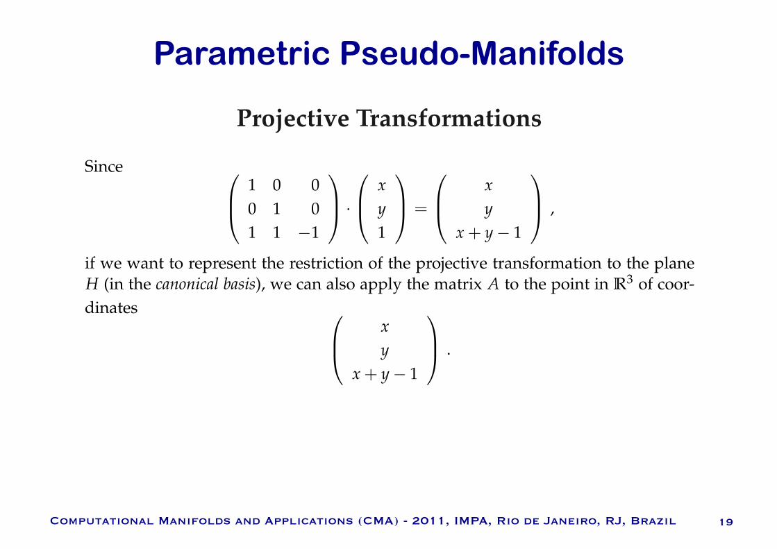
Since
1 0 00 1 01 1 −1
·
x
y
1
=
x
y
x + y − 1
,
if we want to represent the restriction of the projective transformation to the planeH (in the canonical basis), we can also apply the matrix A to the point in R3 of coor-dinates
x
y
x + y − 1
.

Parametric Pseudo-Manifolds
Computational Manifolds and Applications (CMA) - 2011, IMPA, Rio de Janeiro, RJ, Brazil 20
Projective Transformations
Thus, we can define T1 : RP2 → RP2 as T1(s) = A1 · s, for every s ∈ R3, where
A1 =
λ1x1 + λ3x3 λ2x2 + λ3x3 −λ3 · x3
λ1y1 + λ3y3 λ2y2 + λ3y3 −λ3 · y3
λ1 + λ3 λ2 + λ3 −λ3
,
and the coordinates of s ∈ R3 is given with respect to the canonical basis, (e1, e2, e3).

Parametric Pseudo-Manifolds
Computational Manifolds and Applications (CMA) - 2011, IMPA, Rio de Janeiro, RJ, Brazil 21
Projective Transformations
So, if s = (x, y, 1) ∈ Q, then we get t = T1(s) = (x, y, 1) such that x and y are
x =(λ1x1 + λ3x3)x + (λ2x2 + λ3x3)y − λ3x3
(λ1 + λ3)x + (λ2 + λ3)y − λ3
y =(λ1y1 + λ3y3)x + (λ2y2 + λ3y3)y − λ3y3
(λ1 + λ3)x + (λ2 + λ3)y − λ3.

Parametric Pseudo-Manifolds
Computational Manifolds and Applications (CMA) - 2011, IMPA, Rio de Janeiro, RJ, Brazil 22
Projective Transformations
We can proceed in a similar manner to define the map T2 : RP2 → RP2 taking Qonto Q2.
The second step consists of defining the map T2 : RP2 → RP2 taking Q onto Q2.We can proceed as before, but using p1, p2, p3, and p4 instead of q1, q2, q3, and q4,respectively.
The third step consists of defining the map T. This is done by noticing that T1 is abijection, as A1 is invertible. So, T−1
1 maps Q1 onto Q, and hence we define the mapT as
T(p) = (T2 T−11 )(p) = A2 · A−1
1 · p ,
for every p ∈ Q1, where A2 is the matrix associated with the projective transforma-tion T2.
Parametric Pseudo-Manifolds
Computational Manifolds and Applications (CMA) - 2011, IMPA, Rio de Janeiro, RJ, Brazil 23
Projective Transformations
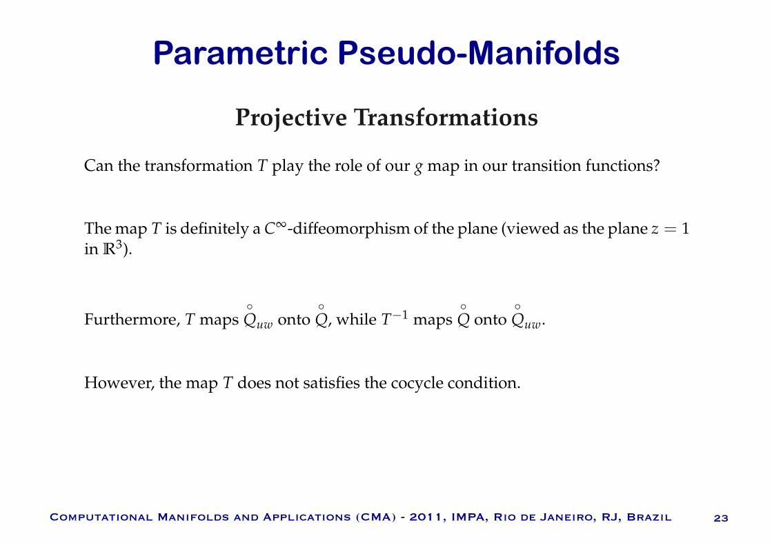
Can the transformation T play the role of our g map in our transition functions?
However, the map T does not satisfies the cocycle condition.
The map T is definitely a C∞-diffeomorphism of the plane (viewed as the plane z = 1in R3).
Furthermore, T mapsQuw onto
Q, while T−1 maps
Q onto
Quw.

Parametric Pseudo-Manifolds
Computational Manifolds and Applications (CMA) - 2011, IMPA, Rio de Janeiro, RJ, Brazil 24
Projective Transformations
To see why, consider a triangle, σ = [u, v, w] of K, such that nu = 5, nv = 6, andnw = 7.
w
v
u
ruw(Quw) = ruv(Quv) =
(0, 0),
cos
−2π
5
, sin
−2π
5
, (1, 0),
cos
2π
5
, sin
2π
5
,
rvu(Qvu) = rvw(Qvw) =(0, 0),
cos
−π
3
, sin
−π
3
, (1, 0),
cos
π
3
, sin
π
3
,
rwv(Qwv) = rwu(Qwu) =
(0, 0),
cos
−2π
7
, sin
−2π
7
, (1, 0),
cos
2π
7
, sin
2π
7
.
By construction,

Parametric Pseudo-Manifolds
Computational Manifolds and Applications (CMA) - 2011, IMPA, Rio de Janeiro, RJ, Brazil 25
Projective Transformations
We definegu : E2 → E2, gv : E2 → E2, and gw : E2 → E2
as the projective maps that takes ruw(Quw), rvu(Qvu), and rwv(Qwv) onto Q, respec-tively, where
Q =(0, 0),
cos
−π
3
, sin
−π
3
, (1, 0),
cos
π
3
, sin
π
3
.
Parametric Pseudo-Manifolds
Computational Manifolds and Applications (CMA) - 2011, IMPA, Rio de Janeiro, RJ, Brazil 26
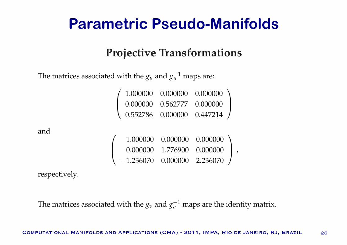
Projective Transformations
The matrices associated with the gv and g−1v maps are the identity matrix.
The matrices associated with the gu and g−1u maps are:
1.000000 0.000000 0.0000000.000000 0.562777 0.0000000.552786 0.000000 0.447214
and
1.000000 0.000000 0.0000000.000000 1.776900 0.000000
−1.236070 0.000000 2.236070
,
respectively.
Parametric Pseudo-Manifolds
Computational Manifolds and Applications (CMA) - 2011, IMPA, Rio de Janeiro, RJ, Brazil 27
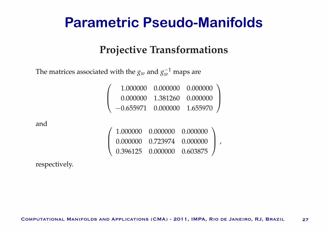
Projective Transformations
The matrices associated with the gw and g−1w maps are
1.000000 0.000000 0.0000000.000000 1.381260 0.000000
−0.655971 0.000000 1.655970
and
1.000000 0.000000 0.0000000.000000 0.723974 0.0000000.396125 0.000000 0.603875
,
respectively.
Parametric Pseudo-Manifolds
Computational Manifolds and Applications (CMA) - 2011, IMPA, Rio de Janeiro, RJ, Brazil 28
Projective Transformations
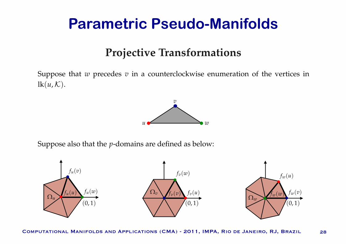
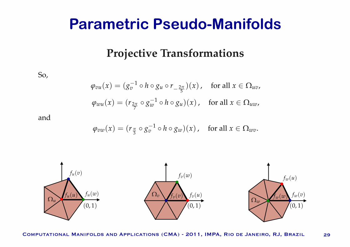
Suppose that w precedes v in a counterclockwise enumeration of the vertices inlk(u,K).
w
v
u
Suppose also that the p-domains are defined as below:
Ωu(0, 1)
fu(v)
fu(w)fu(u)
(0, 1)
Ωv fv(v) fv(u)
fv(w)
(0, 1)Ωw
fw(w)
fw(u)
fw(v)
Parametric Pseudo-Manifolds
Computational Manifolds and Applications (CMA) - 2011, IMPA, Rio de Janeiro, RJ, Brazil 29
Projective Transformations
Ωu(0, 1)
fu(v)
fu(w)fu(u)
(0, 1)
Ωv fv(v) fv(u)
fv(w)
(0, 1)Ωw
fw(w)
fw(u)
fw(v)
So,ϕvu(x) = (g−1
v h gu r− 2π5)(x) , for all x ∈ Ωuv,
ϕwu(x) = (r 2π7 g−1
w h gu)(x) , for all x ∈ Ωuw,
andϕvw(x) = (r π
3 g−1
v h gw)(x) , for all x ∈ Ωwv.

Parametric Pseudo-Manifolds
Computational Manifolds and Applications (CMA) - 2011, IMPA, Rio de Janeiro, RJ, Brazil 30
Projective Transformations
Ωu(0, 1)
fu(v)
fu(w)fu(u)
(0, 1)
Ωv fv(v) fv(u)
fv(w)
(0, 1)Ωw
fw(w)
fw(u)
fw(v)
We can show thatϕuw(Ωwu ∩Ωwv) = Ωuv ∩Ωuw .
So, the statement "if Ωwu ∩Ωwv = ∅ then ϕuw(Ωwu ∩Ωwv) = Ωuv ∩Ωuw" holds. But,it is not the case that ϕvu(x) = (ϕvw ϕwu)(x), for all x ∈ Ωuw ∩ Ωuv. For instance,pick
x = (0.5, 0.5) ∈ (Ωuv ∩Ωuw) .

Parametric Pseudo-Manifolds
Computational Manifolds and Applications (CMA) - 2011, IMPA, Rio de Janeiro, RJ, Brazil 31
Projective Transformations
Indeed,ϕvu(0.5, 0.5) = (0.207988, 0.227109) ,
while(ϕvw ϕwu)(0.5, 0.5) = (0.363339, 0.433479) .
It is worth noticing that map gu is a C∞-diffeomorphism of the plane. Furthermore,
it mapsQuv onto
Q, the canonical quadrilateral. But, the cocycle condition does not
hold.
As a matter of fact, the map gu does not satisfy (gu r 2πnu
g−1u )(x) = r π
3, for q ∈
gu(Ωu).
The map gu does not satisfy (gu ruw)(x) = (r π3 gu ruv)(x), for all x ∈ Ωuv either.

Parametric Pseudo-Manifolds
Computational Manifolds and Applications (CMA) - 2011, IMPA, Rio de Janeiro, RJ, Brazil 32
Complex Functions as Mappings
We will now consider some elementary functions in one complex variable.
These functions can be viewed as mappings from one plane to the other.
So, we will investigate how they can play the role of the g map in our transitionfunctions.
As we shall see, we will not succeed unless we change the geometry of the p-domains.

Parametric Pseudo-Manifolds
Computational Manifolds and Applications (CMA) - 2011, IMPA, Rio de Janeiro, RJ, Brazil 33
Complex Functions as Mappings
Let us recall a few elementary definitions...
A number of the formz = x + i y ,
where x and y are real numbers and i is a number such that i2 = −1 is called acomplex number. The number i is called the imaginary unit, and the numbers x andy are called the real part and the imaginary part of z, denoted by Re(z) and Im(z),respectively.
A complex number z = x + i y is uniquely defined determined by an ordered pair ofreal numbers, (x, y). The first and second entries of the ordered pairs correspond tothe real and imaginary parts of z. Conversely, z = x + i y uniquely determines (x, y).

Parametric Pseudo-Manifolds
Computational Manifolds and Applications (CMA) - 2011, IMPA, Rio de Janeiro, RJ, Brazil 34
Complex Functions as Mappings
The above coordinate plane is called the complex plane or simply the z-plane. The hor-izontal or x-axis is called the real axis and the vertical or y-axis is called the imaginaryaxis.
Since (x, y) can be interpreted as the components of a vector, a complex number
z = x + i y
can be viewed as a vector whose initial point is the origin and whose terminal pointis (x, y).
x
y z = x + i y

Parametric Pseudo-Manifolds
Computational Manifolds and Applications (CMA) - 2011, IMPA, Rio de Janeiro, RJ, Brazil 35
Complex Functions as Mappings
The modulus or absolute value of z = x + i y, denoted by |z|, is the real number
|z| =
x2 + y2 .
A point (x, y) in rectangular coordinates has the polar description, (r, θ), where x, y,r, and θ are related by x = r · cos(θ) and y = r · sin(θ). Thus, a nonzero complexnumber,
z = x + i y ,
can be written as
z = r · cos(θ) + i r · sin(θ) = r ·cos(θ) + i sin(θ)
,
which is the polar form of the complex number z. The angle θ is the argument, arg(z),of z.
Parametric Pseudo-Manifolds
Computational Manifolds and Applications (CMA) - 2011, IMPA, Rio de Janeiro, RJ, Brazil 36
Complex Functions as Mappings
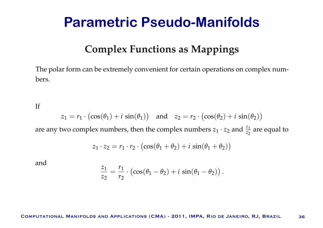
The polar form can be extremely convenient for certain operations on complex num-bers.
Ifz1 = r1 ·
cos(θ1) + i sin(θ1)
and z2 = r2 ·
cos(θ2) + i sin(θ2)
are any two complex numbers, then the complex numbers z1 · z2 and z1z2
are equal to
z1 · z2 = r1 · r2 ·cos(θ1 + θ2) + i sin(θ1 + θ2)
and z1z2
=r1r2
·cos(θ1 − θ2) + i sin(θ1 − θ2)
.
Parametric Pseudo-Manifolds
Computational Manifolds and Applications (CMA) - 2011, IMPA, Rio de Janeiro, RJ, Brazil 37
Complex Functions as Mappings
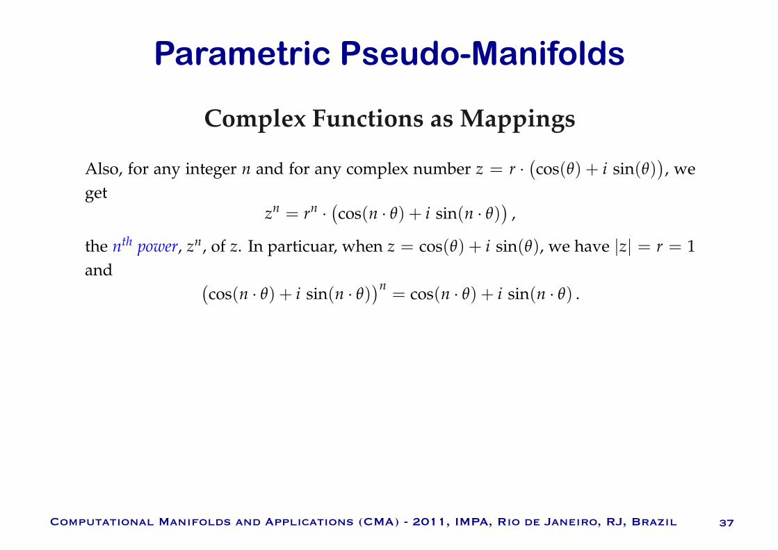
Also, for any integer n and for any complex number z = r ·cos(θ) + i sin(θ)
, we
getzn = rn ·
cos(n · θ) + i sin(n · θ)
,
the nth power, zn, of z. In particuar, when z = cos(θ) + i sin(θ), we have |z| = r = 1and
cos(n · θ) + i sin(n · θ)n = cos(n · θ) + i sin(n · θ) .
Parametric Pseudo-Manifolds
Computational Manifolds and Applications (CMA) - 2011, IMPA, Rio de Janeiro, RJ, Brazil 38
Complex Functions as Mappings
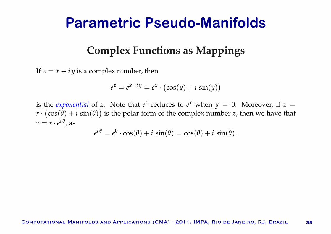
If z = x + i y is a complex number, then
ez = ex+i y = ex ·cos(y) + i sin(y)
is the exponential of z. Note that ez reduces to ex when y = 0. Moreover, if z =r ·
cos(θ) + i sin(θ)
is the polar form of the complex number z, then we have that
z = r · ei θ , asei θ = e0 · cos(θ) + i sin(θ) = cos(θ) + i sin(θ) .

Parametric Pseudo-Manifolds
Computational Manifolds and Applications (CMA) - 2011, IMPA, Rio de Janeiro, RJ, Brazil 39
Complex Functions as Mappings
A function f defined on a set of complex numbers is called a function of a complexvariable z or a complex function. The image w of z will be some complex number,u + i v, i.e.,
w = f (z) = u(x, y) + i v(x, y) ,
where u and v are the imaginary parts of w and are real-valued functions. Obviously,we cannot draw the graph of the complex function w = f (z) with less than four axes.However, we can interpret f as a mapping or transformation from the z-plane to thew-plane.
x
y
u
v
w = u + i v
z = x + i y

Parametric Pseudo-Manifolds
Computational Manifolds and Applications (CMA) - 2011, IMPA, Rio de Janeiro, RJ, Brazil 40
Complex Functions as Mappings
For the functionf (z) = z2 ,
the image of the line Re(z) = 1 is a curve. Indeed, if we write z as = x + i y, then
z2 = (x2 − y2) + i 2xy =⇒ f (z) = u(x, y) + i v(x, y) ,
with u(x, y) = x2 − y2 and v(x, y) = 2xy. Since Re(z) = 1, substituting x = 1 into uand v, we get u = 1− y2 and v = 2y. These parametric equations of a curve in thew-plane.

Parametric Pseudo-Manifolds
Computational Manifolds and Applications (CMA) - 2011, IMPA, Rio de Janeiro, RJ, Brazil 41
Complex Functions as Mappings
Re(z) = 1 f (Re(z))

Parametric Pseudo-Manifolds
Computational Manifolds and Applications (CMA) - 2011, IMPA, Rio de Janeiro, RJ, Brazil 42
Complex Functions as Mappings
Now, let us see some elementary maps.
The mapping f (z) = ez:
In general, if z(t) = x(t) + i y(t), with a ≤ t ≤ b, describes a curve C is the z-plane,then w = f (z(t)) is a parametric representation of the corresponding curve, C, inthe w-plane.
Recall that if z = x + i y then f (z) = ez = ex ·cos(y) + i sin(y)
.

Parametric Pseudo-Manifolds
Computational Manifolds and Applications (CMA) - 2011, IMPA, Rio de Janeiro, RJ, Brazil 43
Complex Functions as Mappings
0.2 0.1 0.0 0.1 0.2
0.0
0.1
0.2
0.3
0.4
0.5
0.6
0.7
v
4 2 0 2 40.0
0.5
1.0
1.5
2.0
2.5
3.0
y
A vertical line segment x = a in the upper half of the z-plane can be described by thecurve z(t) = a + i t, for 0 ≤ t ≤ π. So, we get f (z(t)) = ea · ei t. This means that theimage of the line segment z(t) is a semi-circle with center at w = a and with radiusr = ea.

Parametric Pseudo-Manifolds
Computational Manifolds and Applications (CMA) - 2011, IMPA, Rio de Janeiro, RJ, Brazil 44
Complex Functions as Mappings
0.2 0.1 0.0 0.1 0.2
0.0
0.1
0.2
0.3
0.4
0.5
0.6
0.7
v
4 2 0 2 40.0
0.5
1.0
1.5
2.0
2.5
3.0
y
Similarly, a horizontal line y = b can be parametrized by z(t) = t + i b, with −∞ <t < ∞, and so f (z(t)) = et · ei b. Since arg(w) = b and |w| = et, the image is aray emanating from the origin. Because 0 ≤ arg(z) ≤ π, the image of the entirehorizontal strip, x + i y | −∞ ≤ x ≤ ∞ and 0 ≤ y ≤ π, is the upper half-plane v ≥0.
Parametric Pseudo-Manifolds
Computational Manifolds and Applications (CMA) - 2011, IMPA, Rio de Janeiro, RJ, Brazil 45
Complex Functions as Mappings
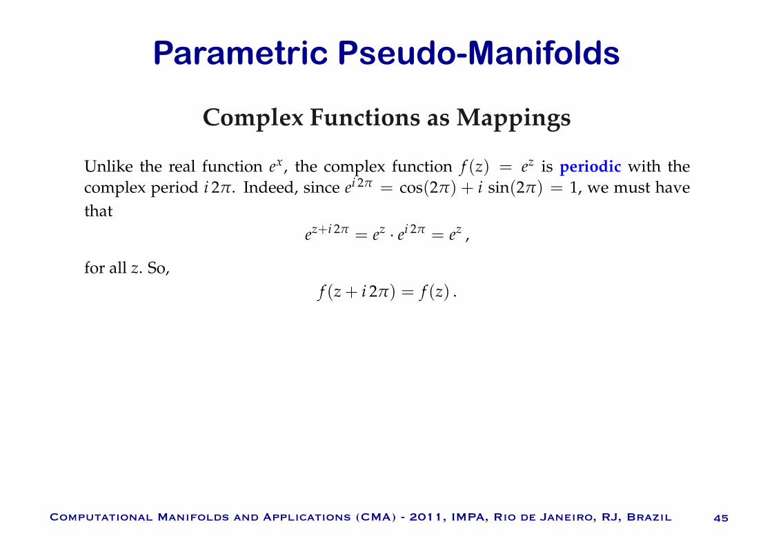
Unlike the real function ex, the complex function f (z) = ez is periodic with thecomplex period i 2π. Indeed, since ei 2π = cos(2π) + i sin(2π) = 1, we must havethat
ez+i 2π = ez · ei 2π = ez ,
for all z. So,f (z + i 2π) = f (z) .
Parametric Pseudo-Manifolds
Computational Manifolds and Applications (CMA) - 2011, IMPA, Rio de Janeiro, RJ, Brazil 46
Complex Functions as Mappings
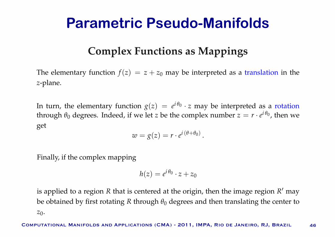
The elementary function f (z) = z + z0 may be interpreted as a translation in thez-plane.
In turn, the elementary function g(z) = ei θ0 · z may be interpreted as a rotationthrough θ0 degrees. Indeed, if we let z be the complex number z = r · ei θ0 , then weget
w = g(z) = r · ei (θ+θ0) .
Finally, if the complex mapping
h(z) = ei θ0 · z + z0
is applied to a region R that is centered at the origin, then the image region R maybe obtained by first rotating R through θ0 degrees and then translating the center toz0.

Parametric Pseudo-Manifolds
Computational Manifolds and Applications (CMA) - 2011, IMPA, Rio de Janeiro, RJ, Brazil 47
Complex Functions as Mappings
For instance,h(z) = i z + 3
maps the horizontal strip−1 ≤ y ≤ 1 onto the vertical strip 2 ≤ x ≤ 4. Indeed, if thehorizontal strip −1 ≤ x ≤ 1 is rotated through 90o (i.e., ei π/2 = i), then the vertical−1 ≤ x ≤ 1 results. Finally, a translation of 3 units to the right yields the verticalstrip 2 ≤ x ≤ 4.

Parametric Pseudo-Manifolds
Computational Manifolds and Applications (CMA) - 2011, IMPA, Rio de Janeiro, RJ, Brazil 48
Complex Functions as Mappings
4 2 0 2 41.0
0.5
0.0
0.5
1.0
x
y
2.0 2.5 3.0 3.5 4.0
4
2
0
2
4
x

Parametric Pseudo-Manifolds
Computational Manifolds and Applications (CMA) - 2011, IMPA, Rio de Janeiro, RJ, Brazil 49
Complex Functions as Mappings
0 1 2 3 4 50
1
2
3
4
5
4 2 0 2 40
1
2
3
4
5
A complex function of the form f (z) = zα, where α is a fixed positive real number,is called a real power function. If z = r · ei θ , then w = f (z) = rα · ei α·θ . Since0 ≤ arg(w) ≤ α · θ0, function f opens or contracts the wedge 0 ≤ arg(z) ≤ θ0 by afactor of α.

Parametric Pseudo-Manifolds
Computational Manifolds and Applications (CMA) - 2011, IMPA, Rio de Janeiro, RJ, Brazil 50
Complex Functions as Mappings
We can show that a circular arc with center at the origin is mapped by f (z) = zα ontoa similar circular arc, and that rays emanating from the origin are mapped by f tosimilar rays.
0 1 2 3 4 50
1
2
3
4
5
4 2 0 2 40
1
2
3
4
5

Parametric Pseudo-Manifolds
Computational Manifolds and Applications (CMA) - 2011, IMPA, Rio de Janeiro, RJ, Brazil 51
Complex Functions as Mappings
Now, let us consider a p-domain, Ωu, where u is a vertex of K such that nu = 5.
Ωu
By definition,
ruv(Quv) =(0, 0),
cos
−2π
5
, sin
−2π
5
, (1, 0),
cos
2π
5
, sin
2π
5
.

Parametric Pseudo-Manifolds
Computational Manifolds and Applications (CMA) - 2011, IMPA, Rio de Janeiro, RJ, Brazil 52
Complex Functions as Mappings
What is the image of ruv(Quv) under the map f (z) = zα, where α = 56 ?
Is that the case that f (ruv(Quv)) = Q?
Ωu
Note that
f (0 + i 0) = 0 , f (1 + i 0) = 1 , f
ei (− 2π5 )
= ei (− π
3 ), and f
ei 2π5
= ei π
3 .

Parametric Pseudo-Manifolds
Computational Manifolds and Applications (CMA) - 2011, IMPA, Rio de Janeiro, RJ, Brazil 53
Complex Functions as Mappings
Unfortunately, NO!
The region f (ruv(Quv)) will look like the picture below:
This is because f (z) = zα scales the modulus of z = r · (cos(θ) + i sin(θ)): r becomesrα.
Parametric Pseudo-Manifolds
Computational Manifolds and Applications (CMA) - 2011, IMPA, Rio de Janeiro, RJ, Brazil 54
Complex Functions as Mappings
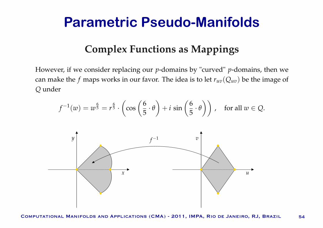
However, if we consider replacing our p-domains by "curved" p-domains, then we
can make the f maps works in our favor. The idea is to let ruv(Quv) be the image of
Q under
f−1(w) = w6
5 = r6
5 ·
cos
6
5· θ
+ i sin
6
5· θ
, for all w ∈ Q.
x
y
u
vf−1

Parametric Pseudo-Manifolds
Computational Manifolds and Applications (CMA) - 2011, IMPA, Rio de Janeiro, RJ, Brazil 55
Complex Functions as Mappings
The picture below illustrates the shape of the p-domain Ωu (left) obtained by apply-ing f−1 to Q and then rotating f−1(Q) around the origin. The result is a "curved"p-domain (right).
Ωu Ωu

Parametric Pseudo-Manifolds
Computational Manifolds and Applications (CMA) - 2011, IMPA, Rio de Janeiro, RJ, Brazil 56
Complex Functions as Mappings
Ωu
fu(v)
fu(w)fu(u) Ωv fv(v) fv(u)
fv(w)
Ωwfw(w)
fw(u)
fw(v)

Parametric Pseudo-Manifolds
Computational Manifolds and Applications (CMA) - 2011, IMPA, Rio de Janeiro, RJ, Brazil 57
Complex Functions as Mappings
The map Π is a C∞-diffeomorphism. So, working with polar coordinates is fine aswell.
So,gu(x, y) = (Π−1 Γu Π)(x, y) ,
whereΠ : E2 − (0, 0)→ R+ × ]− π , π [
is the map that converts Cartesian coordinates to polar coordinates, Π(x, y) = (r, θ),and
Γu : R+ × ]− π , π [ → R+ × ]− π , π [
is the mapΓu(r, θ) =
r
nu6 ,
nu6
· θ
.

Parametric Pseudo-Manifolds
Computational Manifolds and Applications (CMA) - 2011, IMPA, Rio de Janeiro, RJ, Brazil 58
Complex Functions as Mappings
Indeed, for every (u, w) ∈ K,
ϕwu : Ωuw → Ωwu ,
where
ϕwu(x) =
x if u = w,r−1
wu g−1w h gu ruw
(x) if u = w,
for every x ∈ Ωuw.
Note that the previous g maps are defined in E2 − (0, 0). The fact that (0, 0) doesnot belong to the domain of g is not a problem, as (0, 0) is not part of a gluing domain,except when the gluing domain is the p-domain itself. But, in this case, the transitionmap is defined as the identity map, rather than in terms of the g maps. So, we aresafe!
Parametric Pseudo-Manifolds
Computational Manifolds and Applications (CMA) - 2011, IMPA, Rio de Janeiro, RJ, Brazil 59
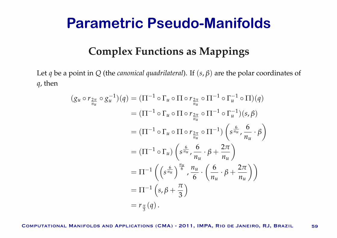
Complex Functions as Mappings
Let q be a point in Q (the canonical quadrilateral). If (s, β) are the polar coordinates ofq, then
(gu r 2πnu g−1
u )(q) = (Π−1 Γu Π r 2πnuΠ−1 Γ−1
u Π)(q)
= (Π−1 Γu Π r 2πnuΠ−1 Γ−1
u )(s, β)
= (Π−1 Γu Π r 2πnuΠ−1)
s
6nu ,
6nu
· β
= (Π−1 Γu)
s6
nu ,6
nu· β +
2π
nu
= Π−1
s6
nu
nu6 ,
nu6
·
6nu
· β +2π
nu
= Π−1
s, β +π
3
= r π3(q) .

Parametric Pseudo-Manifolds
Computational Manifolds and Applications (CMA) - 2011, IMPA, Rio de Janeiro, RJ, Brazil 60
Complex Functions as Mappings
If (t, α) are the polar coordinates of p and if −θ is the angle of rotation of ruw, then
(t, α− θ) and
t, α− θ − 2π
nu
are the polar coordinates of ruw(p) and ruv(p), respectively, as we assumed (in ourexample) that w precedes v in a counterclockwise enumeration of the vertices oflk(u,K).
w
v
u
Let p be a point in Ωu − (0, 0).

Parametric Pseudo-Manifolds
Computational Manifolds and Applications (CMA) - 2011, IMPA, Rio de Janeiro, RJ, Brazil 61
Complex Functions as Mappings
So,
(gu ruw)(p) = (Π−1 Γu Π ruw)(p)
= (Π−1 Γu)(t, α− θ)
= (Π−1)
tnu6 ,
nu6
· (α− θ)
.

Parametric Pseudo-Manifolds
Computational Manifolds and Applications (CMA) - 2011, IMPA, Rio de Janeiro, RJ, Brazil 62
Complex Functions as Mappings
In turn,
(r π3 gu ruv)(p) = (r π
3Π−1 Γu Π ruv)(p)
= (r π3Π−1 Γu)
t, α− θ − 2π
nu
= (r π3Π−1)
t
nu6 ,
nu6
·
α− θ − 2π
nu
= (r π3Π−1)
t
nu6 ,
nu6
· (α− θ)− π
3
= Π−1
tnu6 ,
nu6
· (α− θ)
= (gu ruw)(p) .

Parametric Pseudo-Manifolds
Computational Manifolds and Applications (CMA) - 2011, IMPA, Rio de Janeiro, RJ, Brazil 63
Complex Functions as Mappings
(3) The gu map satisfies (gu r 2πnu g−1
u )(q) = r π3(q), where q ∈ gu(Ωu).
So, the gu map satisfies the following four conditions:
(4) If fu(w) precedes fu(v) in a counterclockwise enumeration of the vertices oflk(u,K), then (gu ruw)(p) = (r π
3 gu ruv)(p), for every point p in the gluing
domain Ωuw.
(2) The gu map takes ruw(Ωuw) ontoQ, for every (u, w) ∈ K.
(1) The gu map is a Ck-diffeomorphism of E2 − (0, 0), for every u ∈ I.
Parametric Pseudo-Manifolds
Computational Manifolds and Applications (CMA) - 2011, IMPA, Rio de Janeiro, RJ, Brazil 64
Complex Functions as Mappings
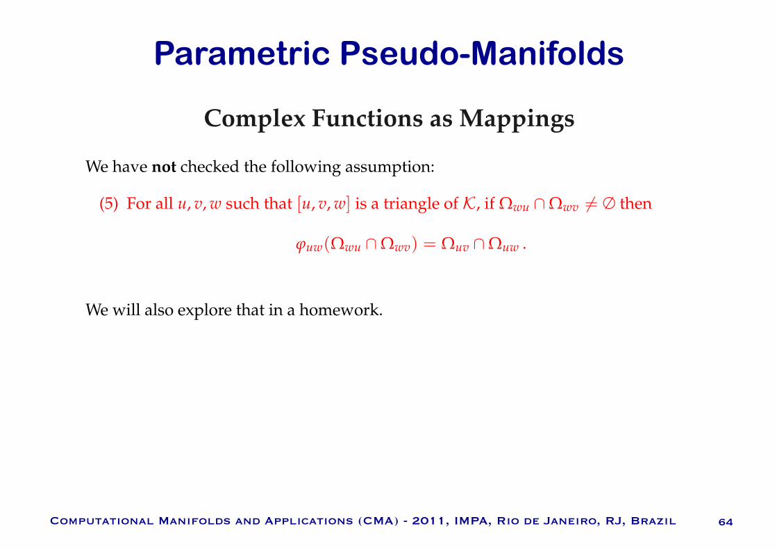
We have not checked the following assumption:
(5) For all u, v, w such that [u, v, w] is a triangle of K, if Ωwu ∩Ωwv = ∅ then
ϕuw(Ωwu ∩Ωwv) = Ωuv ∩Ωuw .
We will also explore that in a homework.