introduction to comsol multiphysics san diego, ca september 20, 2005 mina sierou, ph.d. comsol inc
Post on 19-Dec-2015
241 views
TRANSCRIPT

Introduction to COMSOL Multiphysics
San Diego, CASeptember 20, 2005
Mina Sierou, Ph.D.Comsol Inc.

Contents
Morning Session
• Introduction
• Demonstration of the modeling procedure
• Workshop: Electro-thermal analysis of semiconductor device
– 3D stationary
– 3D parametric
• Workshop: Mesh Control
Afternoon Session• Hands-on modeling workshops:
– Flow over a Backstep
– Electric Impedance Center
– Thermal Stresses in a Layered
Plate
– MEMS Thermal Bilayer Valve
– Using Interpolation Function
– Using Mapped Meshes

COMSOL – The company
• Founded 1986• Development of FEMLAB®
/COMSOL Multiphysics (in Sweden)
• Business: software, support,
courses, consulting
• Today, 120 employees worldwide. Offices in US (Boston, L.A.), UK, Germany, France, Sweden, Finland, Norway, and Denmark
• Distributor network covering the rest of the world

Highlights of COMSOL Multiphysics
• General purpose Multiphysics FEA code
• MATLAB/COMSOL Script integration– COMSOL Multiphysics can be run stand-alone
– or with MATLAB for richer set of functions
– Can use MATLAB or COMSOL Script as a scripting language
• Easy to learn and use• Extremely adaptable and extensible

The COMSOL Multiphysics Product Line
And introducing…

COMSOL Script

CAD import module + Mesh import
• In 3.2 we can import IGES, STEP, SAT, X_T, Pro/E, CATIA,Inventor, VDA files with:– More than 1000 faces
– Sliver faces, spikes, short edges and other errors

COMSOL Multiphysics Users
• Rice, Texas A & M, UH
• UT Austin, UT Arlington
• Stanford, Caltech, JPL
• UC’s, UW
• MIT, Harvard, Princeton…
• Y NL
– Y=LA,LL,LB,PN, Sandia
• NASA research centers
• NIST, NREL, USGS, SWRI
• NIH
• Shell, Exxon Mobil
• Schlumberger, Dow Chemicals
• Northrop-Grumman, Raytheon
• Applied Materials, Agilent
• Boeing, Lockheed-Martin
• GE, 3M
• Merck, Roche
• Procter and Gamble, Gillette
• Energizer, Eveready
• Hewlett-Packard, Microsoft, Intel
• Nissan, Sony, Toshiba
• ABB, Volkswagen, GlaxoSmithKline
• Philip-Morris

Mathematical Modeling
• Mathematical description of physical phenomena translates into equations
• Description of changes in space and time results in Partial Differential Equations (PDE’s)
• Complex geometries and phenomena require modeling with complex equations and boundary conditions
• Resulting PDEs rarely have analytical solutions
Numerical tools are necessary

Material Balances
zFyxjjyx
jjzxjjzyt
uzyx
zzz
yyyxxx
)(
)()(
Fz
jj
y
jj
x
jj
t
u zzzyyyxxx
Fz
j
y
j
x
j
t
u zyx
Ft
u
j
Material balances are usually described by an equation of the form
where j is the flux vector and F a source term

General PDE Form
Ft
uda
Ru
RG
T
0
n
inside domain
on domain boundary
Example: For Poisson’s equation, the corresponding general form implies
uyux .uR
All other coefficients are 0. (For later, note: )
1F
n

Coefficient Form PDE
fauuuuct
uda
)(
rhu
hgquuuc T )(n
inside subdomain
on boundary
Example: Poisson’s equation 1 u
0u
inside subdomain
on subdomain boundary
(Implies c=f=h=1 and all other coefficients are 0.)
a
ud F
t
If equation is linear, the general form can be expanded into a coefficient form:
transforms into

Multiphysics Capabilities
• Very different physical phenomena can be described with the same general equations
• Coupling of different physical formulations (multiphysics) is thus straightforward in COMSOL Multiphysics
• Resulting systems of equations can be solved sequentially or in a fully-coupled formulation
• Extended Multiphysics: Physics in different geometries can be easily combined
• Coupling variables can also be used to link different physics or geometries

Worked Example – A Simple Fin
Purpose of the model
• Explain the modeling procedure in COMSOL Multiphysics
• Show the use of pre-defined application modes in physics mode
• Introduce some very useful features for control of modeling results

Problem definition
• Heat transfer by conduction (Heat Conduction application mode)
• Linear equation, stationary solution
• Different thermal conductivities can be defined in different subdomains

Problem Definition
symmetry
Step 1
Step 2 0 Tk
1k
2k12 10 kk
1T
2T 0 nTk
1k
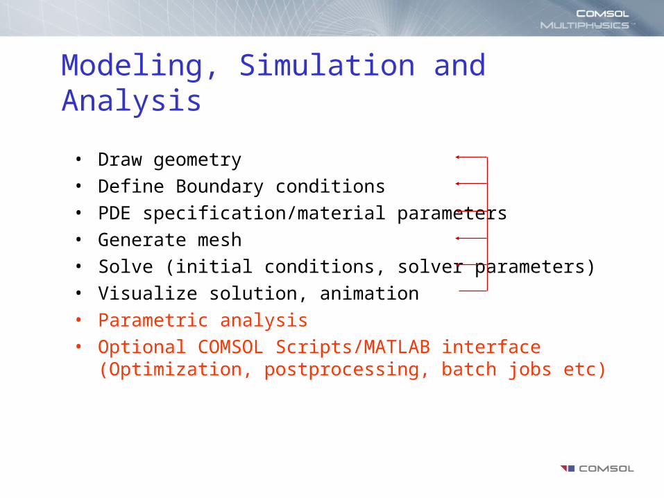
Modeling, Simulation and Analysis
• Draw geometry
• Define Boundary conditions
• PDE specification/material parameters
• Generate mesh
• Solve (initial conditions, solver parameters)
• Visualize solution, animation
• Parametric analysis
• Optional COMSOL Scripts/MATLAB interface (Optimization, postprocessing, batch jobs etc)

Results
Example:
Thermal effects in an electric conductor

Introduction
• The phenomena in this example involve the coupling of thermal and electronic current balances.
• The ohmic losses due to the device’s limited conductivity generate heat, which increases the conductor’s temperature and thus also changes the material’s conductivity. This implies that a 2-way multiphysics coupling is in play.
• Parameterization to study temperature as function of different electrode potentials
Purpose: Introduce you to the general concepts of multiphysics modeling methodology in COMSOL Multiphysics
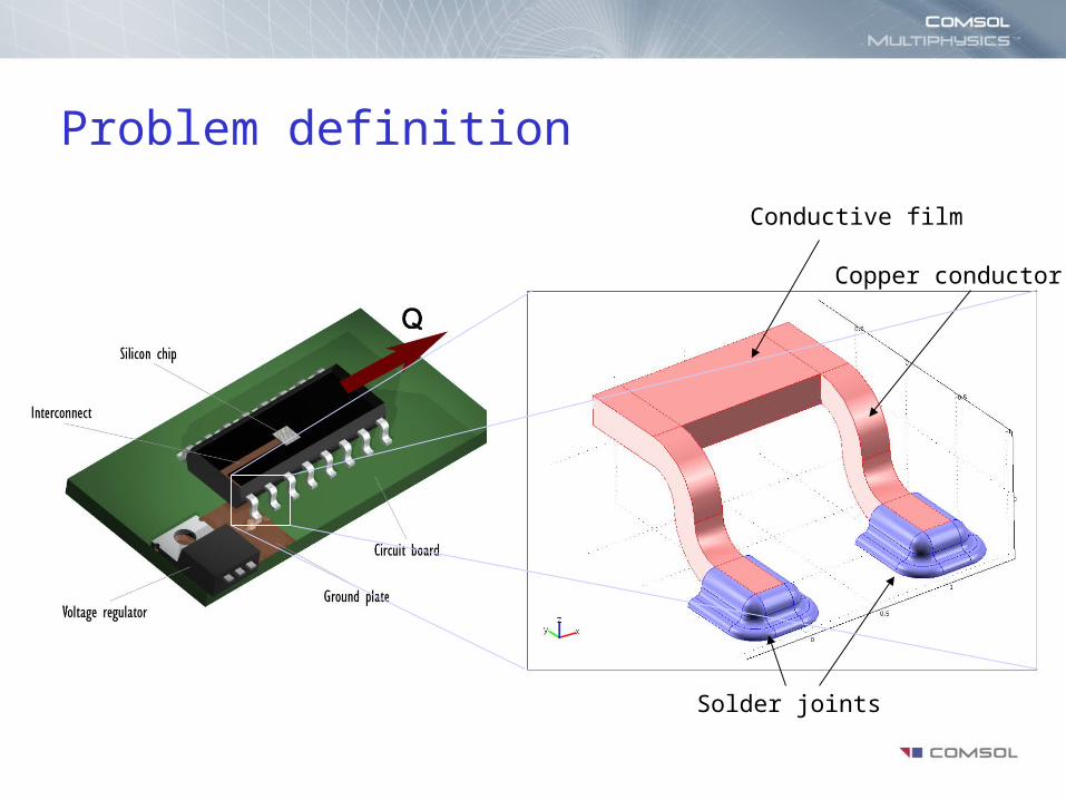
Problem definition
Conductive film
Copper conductor
Solder joints

Problem definition
Heat balance: Current balance:
-·( V) = 0
2VQ 00 1
1
TT
( )k T Q

Second Example: Mesh Control
• Automated mesh generator– Suitable for some problems– But not always optimal
• How can you to create a non-uniform mesh?– Mesh parameters menu– Mesh Quality
• Thin Geometries– Scale problem / mesh / Unscale
• Workshop Exercise: Mesh Control– Mesh parameters menu– Displaying Mesh Quality

Lunch Break
• Back in 1 hour
Interpolation functions
• Interpolation of measured data is commonly necessary when analytical expressions for material properties are not available
• New feature in 3.1
• You can use interpolation function directly in the GUI (without the need for MATLAB)
• Data can be entered from a table (for 1D interpolation) or from a text file (for multidimensional interpolation)
• Example: Thermal conductivity as a function of temperature

Example: Flow over a backstep

Thermal Flow over a Backstep
• Single physics– Fluid dynamics
• Multiphysics– You could add heat transfer and establish temperature profiles
• Aim of the model– To give an overview of the modeling process in COMSOL
Multiphysics– Standard CFD benchmark– Use both regular triangular and mapped meshes and compare the
solution for various mesh densities
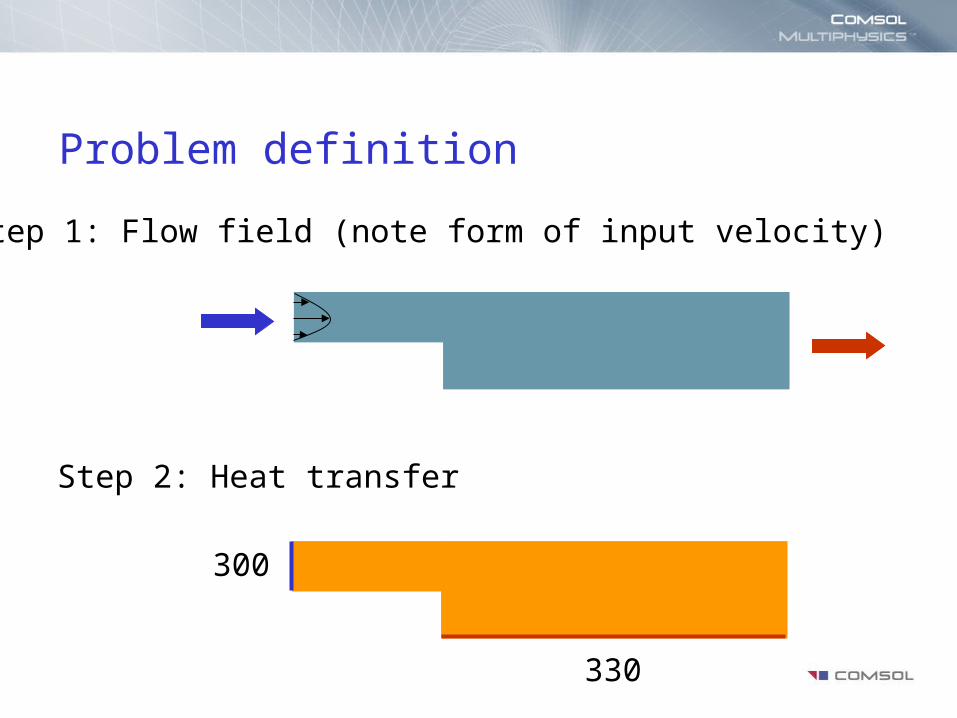
Problem definition
Step 1: Flow field (note form of input velocity)
Step 2: Heat transfer
300
330

Results: Stationary velocity profile

Results: Transient temperature profile
t=5 t=10
t=15 t=20
Concluding remarks
• The model is simple to define and solve in COMSOL Multiphysics.
• The applications can be solved simultaneusly or sequentially and for stationary or time dependent problems.
• Different Reynolds numbers can be easily sampled

Example: Electric Impedance Sensor
Introduction
• Electric impedance measurement techniques are used for imaging and detection– Geophysical imaging
– Non-destructive testing
– Medical imaging (Electrical Impedance Tomography)
• Applying voltage to an object or a matrix containing different materials and measuring the resulting potentials or current densities
• Frequency range: 1Hz < f < 1GHz
Main points
• Use of Electromagnetics Module, Small Currents Application Mode
• Different Subdomains with different physical properties
• Logical expressions can be used to modify the geometry
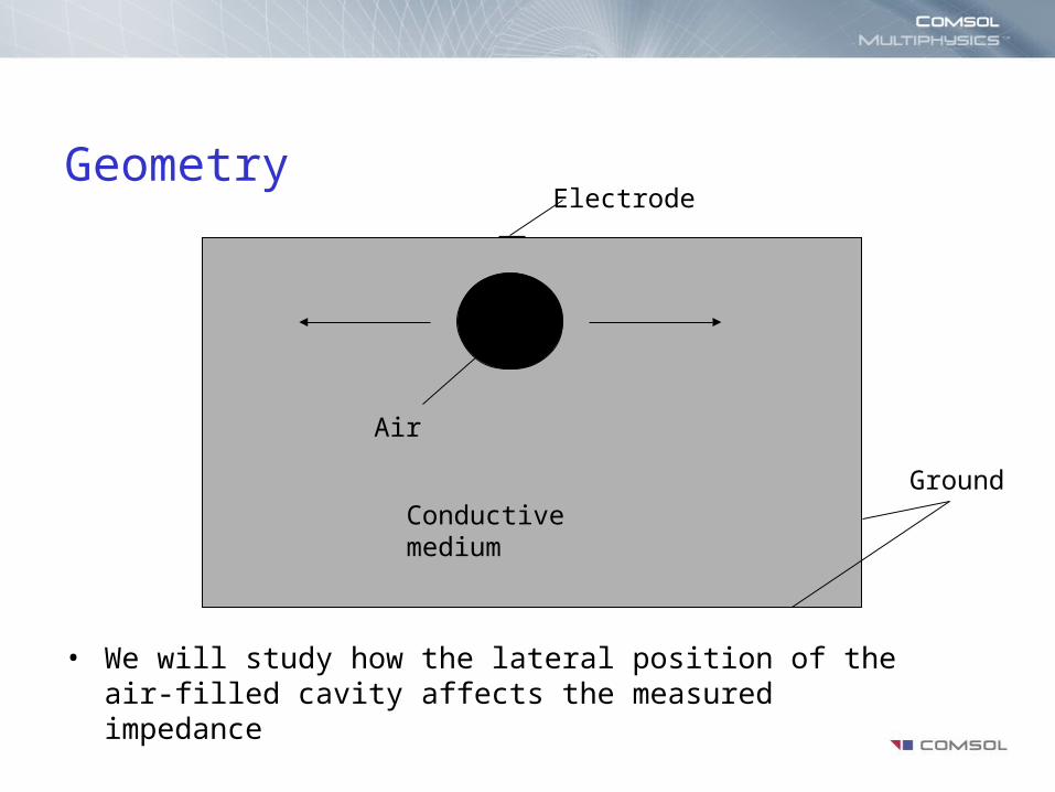
Geometry
• We will study how the lateral position of the air-filled cavity affects the measured impedance
Air
Electrode
Conductive mediumGround
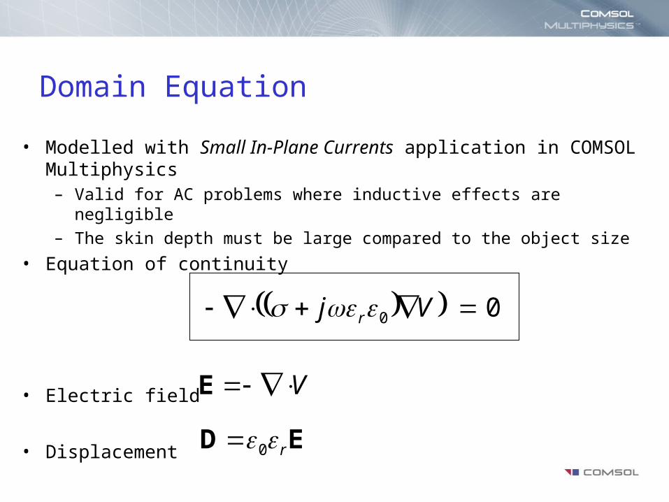
Domain Equation
• Modelled with Small In-Plane Currents application in COMSOL Multiphysics– Valid for AC problems where inductive effects are negligible
– The skin depth must be large compared to the object size
• Equation of continuity
• Electric field
• Displacement
00 Vj r
VΕ
ED r0

Equations and boundary conditions
00 Vj r
A1 nJJn
0V
0Jn

Results: Current distribution [on a dB scale]
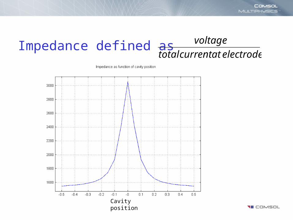
Impedance defined aselectrodeatcurrenttotal
voltage
Cavity position

Results: Impedance phase angle
Cavity position
Example:Thermal Stresses in a Layered Plate

Geometry
coating
substrate
carrier
1. The coating is deposited on the substrate, at 800 °C
2. The temperature is lowered to 150 °C -> thermal stresses in the coating/substrate assembly.
3. The coating/substrate assembly is epoxied to a carrier plate.
4. The temperature is lowered down to 20 °C.
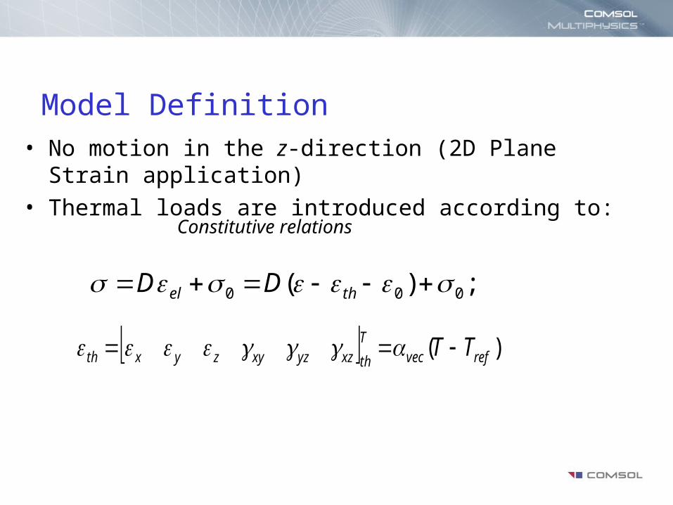
Model Definition• No motion in the z-direction (2D Plane Strain application)
• Thermal loads are introduced according to:
;)( 000 thel DD
Constitutive relations
)( refvecT
thxzyzxyzyxth TT

Results: First step
• Result after depositing the coating on the substrate and lowering the temperature to 150 °C
• The figure shows the stress in the x direction
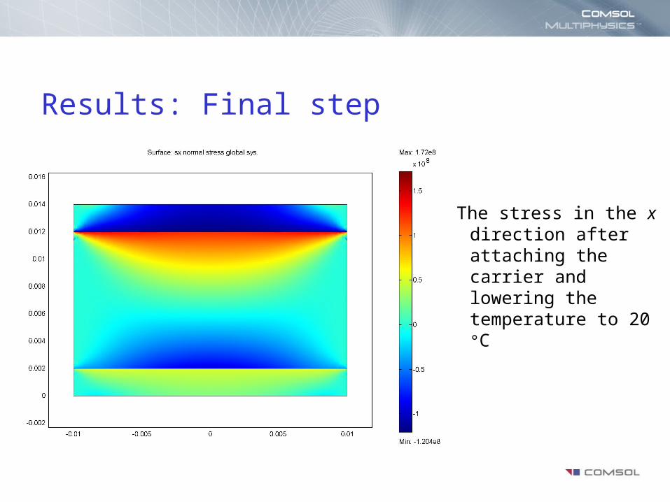
Results: Final step
The stress in the x direction after attaching the carrier and lowering the temperature to 20 °C
Example: Rapid thermal annealing

Rapid Thermal Anneal –the device
• Important process step in semiconductor processing
• Rapidly heat up Silicon wafer to 1000 degrees C for 10 seconds
Heater
Detector
Silicon wafer
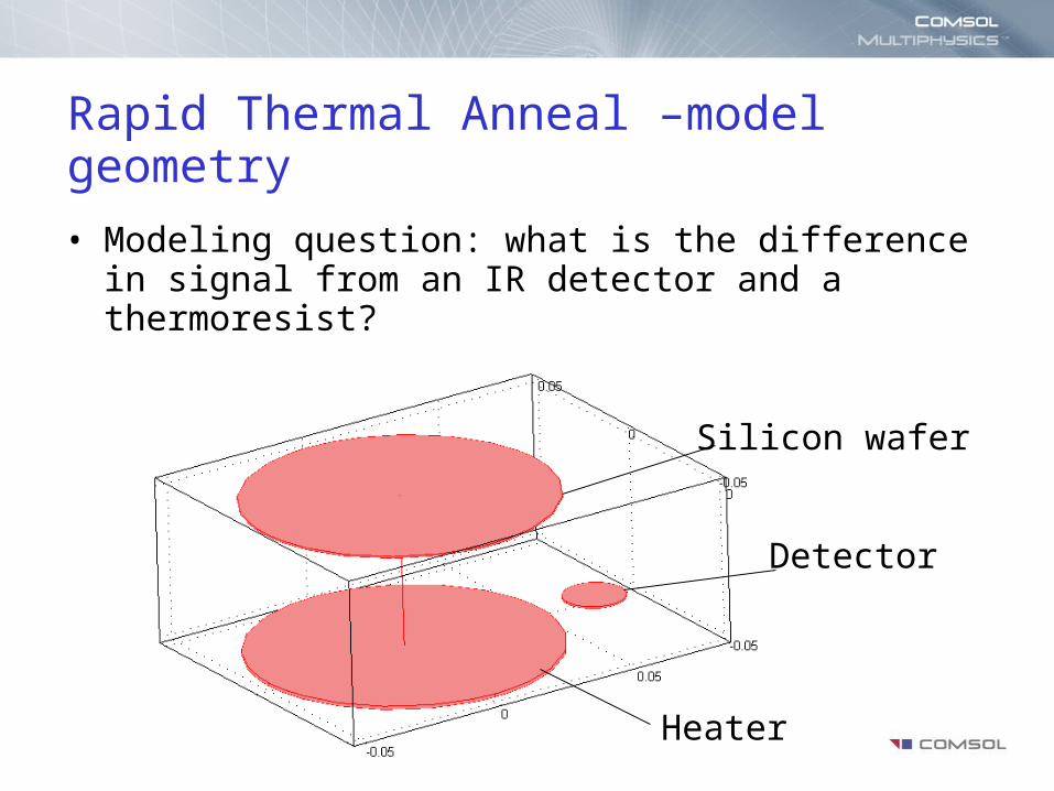
Rapid Thermal Anneal –model geometry
• Modeling question: what is the difference in signal from an IR detector and a thermoresist?
)1()(
)(4
0
TJ
Tkn
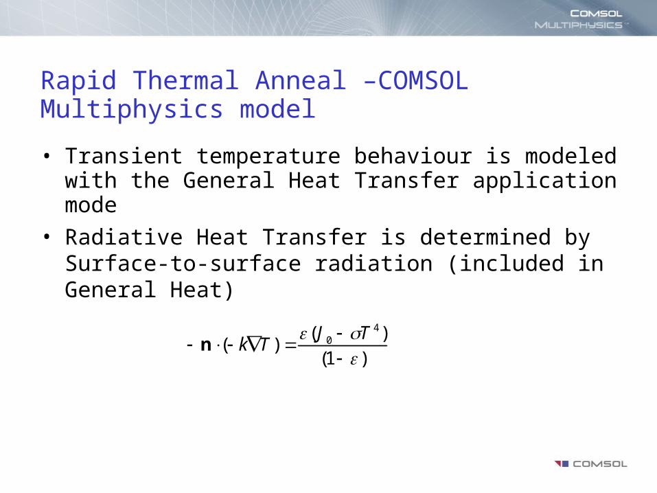
Rapid Thermal Anneal –COMSOL Multiphysics model
• Transient temperature behaviour is modeled with the General Heat Transfer application mode
• Radiative Heat Transfer is determined by Surface-to-surface radiation (included in General Heat)
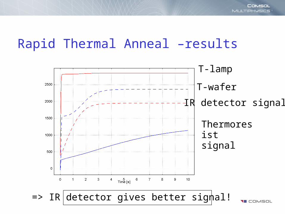
T-lamp
T-wafer
IR detector signal
Thermoresist signal
=> IR detector gives better signal!
Rapid Thermal Anneal –results
Example: MEMs Thermal Bilayer Valve
Thermal Bilayer Valve
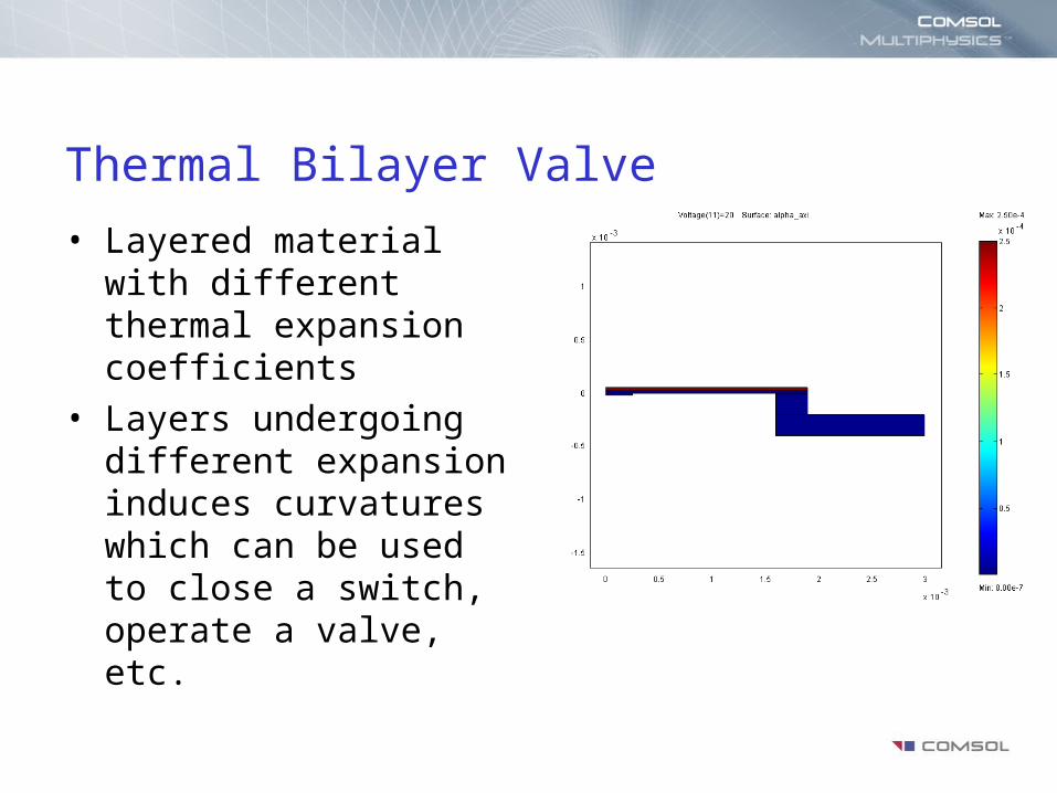
• Layered material with different thermal expansion coefficients
• Layers undergoing different expansion induces curvatures which can be used to close a switch, operate a valve, etc.

Thermal Bilayer Valve
• Structural deformation from thermal expansion
• Structural buckling
• Thermal conduction
• Heat source: Joule heating
• Current from DC conductive – Axisymmetric
• Meshing Thin Layers

Using Mapped Meshes
• Feature introduced in FEMLAB 3.1
• 2D quadrilateral elements can be generated by using a mapping technique (defined on a unit square)
• Best suited for fairly regular domains (connected, at least four boundary segments, no isolated vertices) but irregular geometry can also often be modified/divided in smaller regular ones
• 2D mesh can then extruded/revolved to generate 3D brick elements

Example: Printed Circuit Board
Printed Circuit Board
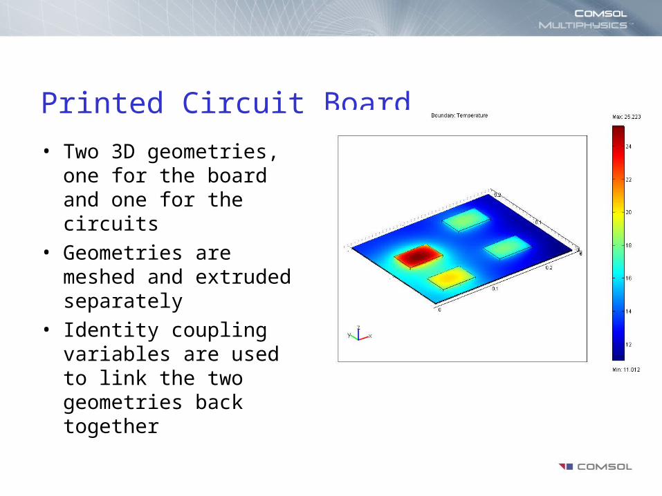
• Two 3D geometries, one for the board and one for the circuits
• Geometries are meshed and extruded separately
• Identity coupling variables are used to link the two geometries back together