introduction to conditional logistic regression...
TRANSCRIPT
Introduction to Conditional Logistic Regression Analysis
Ho Kim
School of Public Health
Seoul National University
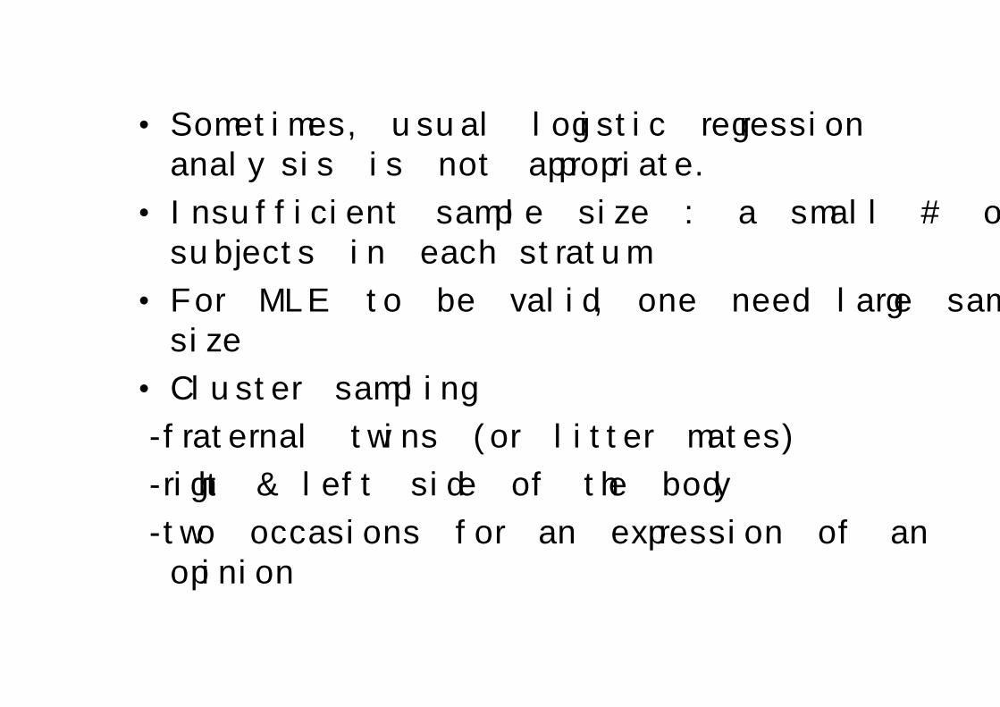
• Sometimes, usual logistic regression analysis is not appropriate.
• Insufficient sample size : a small # of subjects in each stratum
• For MLE to be valid, one need large sample size
• Cluster sampling
-fraternal twins (or litter mates)
-right & left side of the body
-two occasions for an expression of an opinion
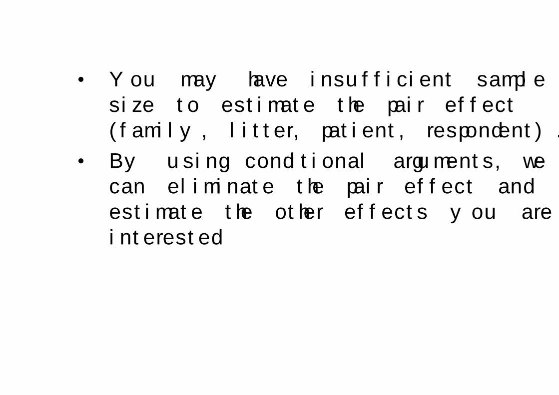
• You may have insufficient sample size to estimate the pair effect (family, litter, patient, respondent).
• By using conditional arguments, we can eliminate the pair effect and estimate the other effects you are interested
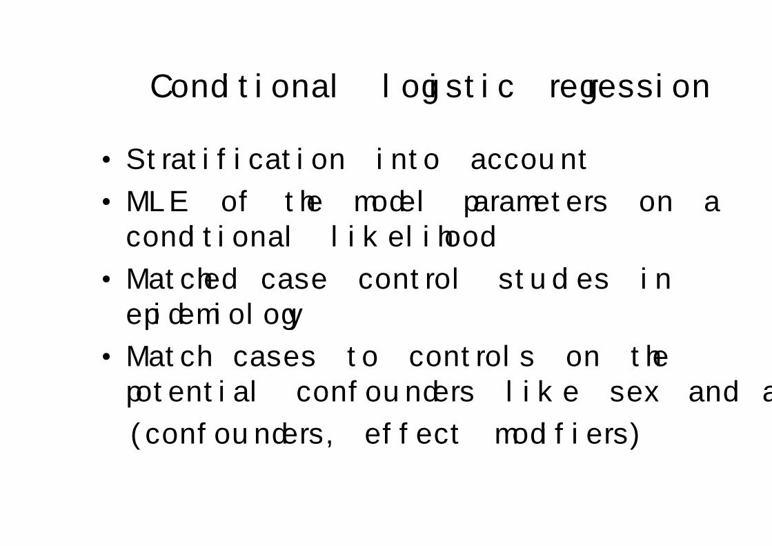
Conditional logistic regression
• Stratification into account
• MLE of the model parameters on a conditional likelihood
• Matched case control studies in epidemiology
• Match cases to controls on the potential confounders like sex and age
(confounders, effect modifiers)
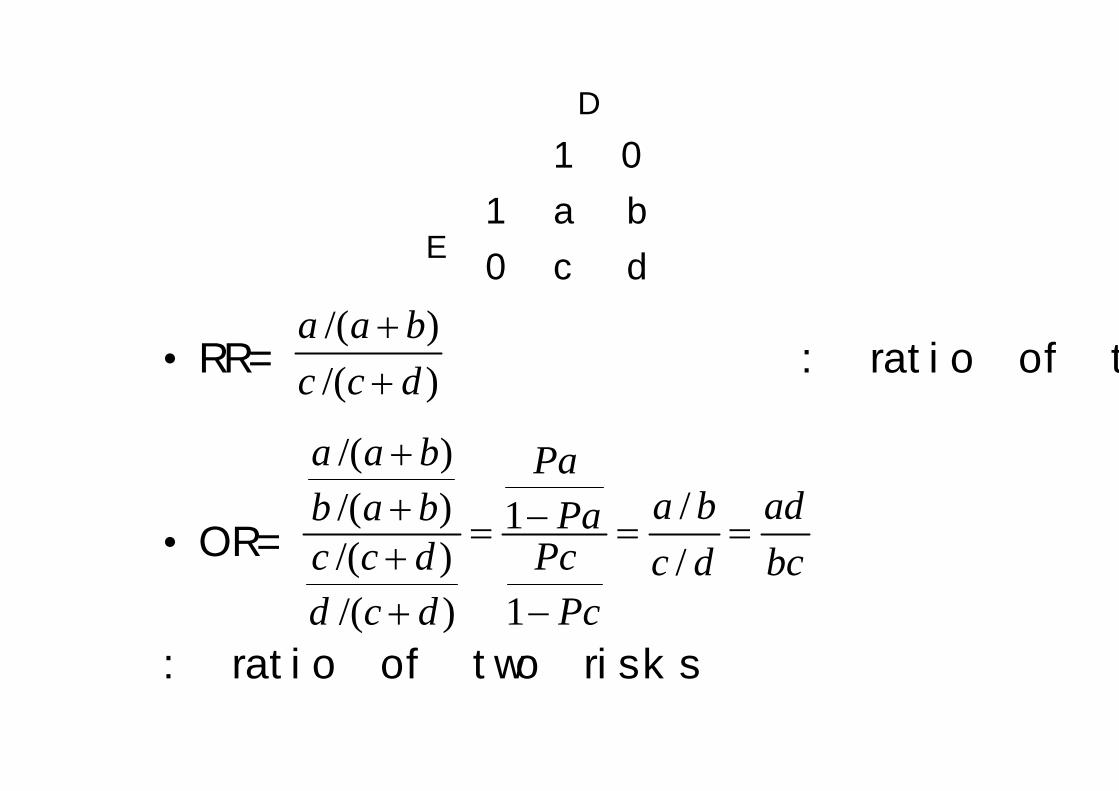
dc0
ba1
01
D
E
/( )/( )
a a bc c d
++• RR= : ratio of two risks
• OR=
: ratio of two risks
/( )//( ) 1
/( ) //( ) 1
a a b Paa b adb a b Pa
c c d Pc c d bcd c d Pc
++ −= = =++ −
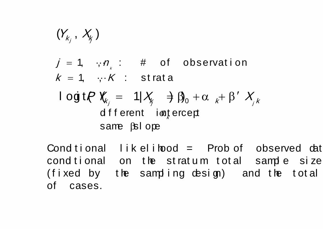
data( , , )j jk k kY X Z
==1, , : # o f o b servatio n
1, , : strata k
j n
k k
αβ
β α β ′= + +0
different intercept
sam e slope
( , )
k
j jk k k kg X Z X
( , )j jk kY X
==
1, , : # of observation
1, , : strata k
j n
k K
αβ
β α β ′= = + +0
different intercept
same slope
logit( ( 1| ))
k
j j jk k k kP Y X X
Conditional likelihood = Prob of observed data conditional on the stratum total sample size (fixed by the sampling design) and the total # of cases.
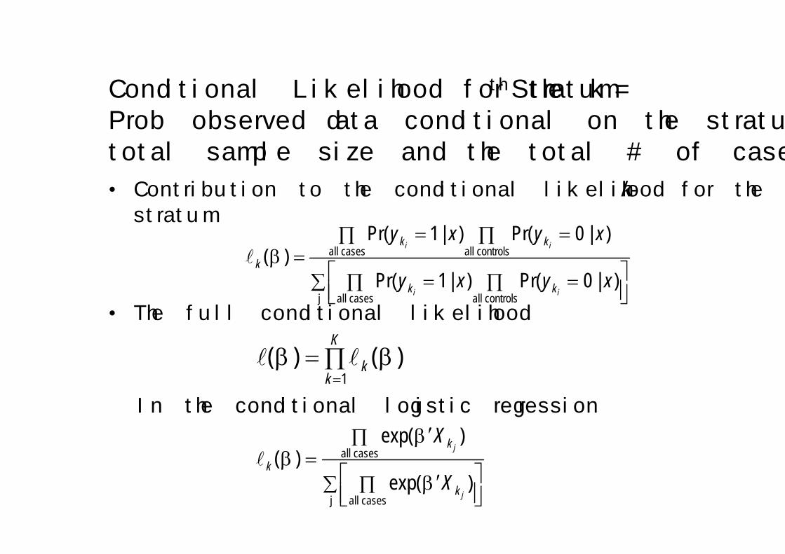
Conditional Likelihood for the kth Stratum=Prob observed data conditional on the stratum total sample size and the total # of cases
• Contribution to the conditional likelihood for the k-stratum
• The full conditional likelihood
In the conditional logistic regression
k
β= =∏ ∏
= = =∑ ∏ ∏
all cases all controls
j all cases all controls
Pr( 1| ) Pr( 0 | )( )
Pr( 1| ) Pr( 0 | )
i i
i i
k k
k
k k
y x y x
y x y x
β β=
= ∏1
( ) ( )K
kk
ββ
β
∏
∑ ∏
′=
′
all cases
j all cases
exp( )( )
exp( )
j
j
k
k
k
X
X
β= =∏ ∏
= = =∑ ∏ ∏
all cases all controls
j all cases all controls
Pr( 1| ) Pr( 0 | )( )
Pr( 1| ) Pr( 0 | )
i i
i i
k k
k
k k
y x y x
y x y x
β β=
= ∏1
( ) ( )K
kk
ββ
β
∏
∑ ∏
′=
′
all cases
j all cases
exp( )( )
exp( )
j
j
k
k
k
X
X
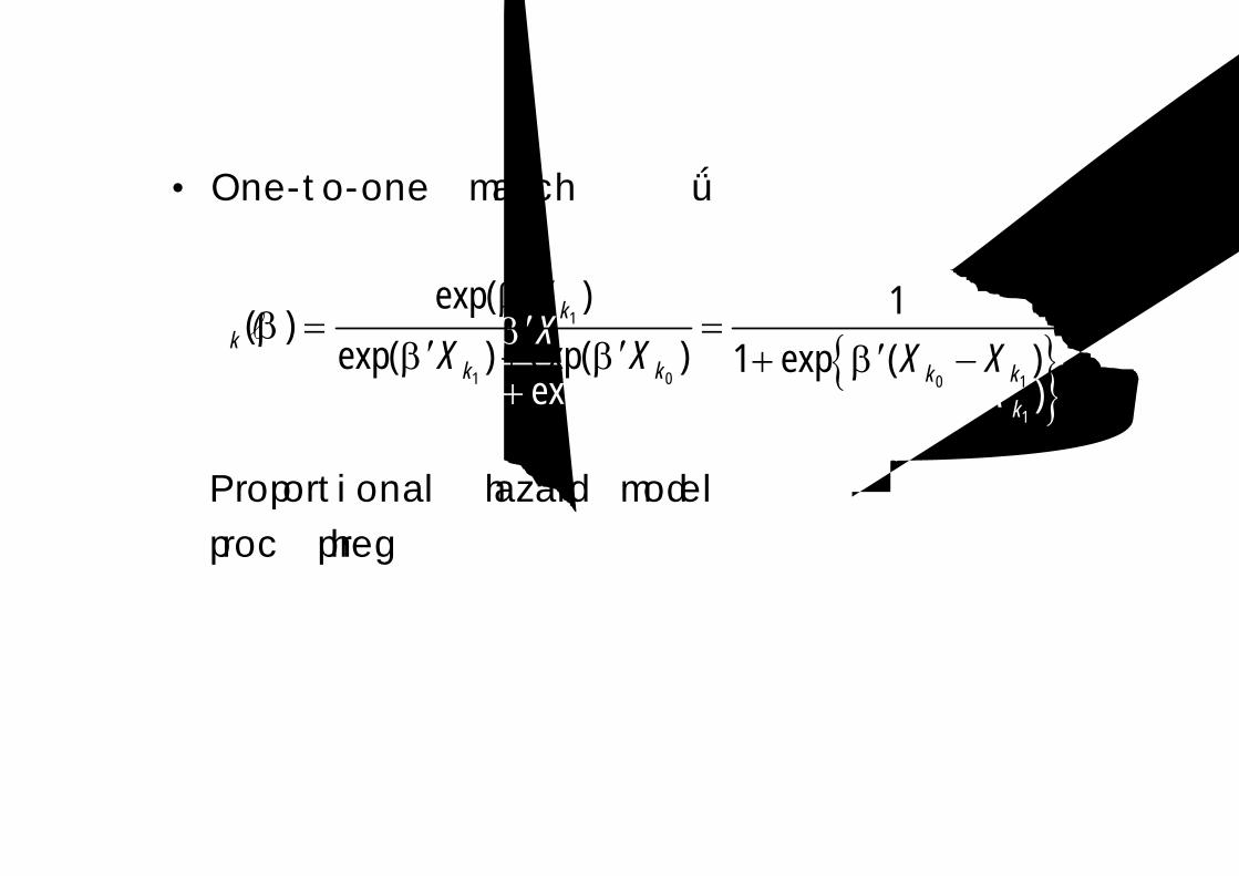
• One-to-one match 의 경우
Proportional hazard model 과 동일
→proc phreg으로 풀 수 있다
{ }β
ββ β β
′= =
′ ′+ ′+ −1
1 0 0 1
exp( ) 1( )exp( ) exp( ) 1 exp ( )
kk
k k k k
XX X X X
{ }β
ββ β β
′= =
′ ′+ ′+ −1
1 0 0 1
exp( ) 1( )exp( ) exp( ) 1 exp ( )
kk
k k k k
XX X X X
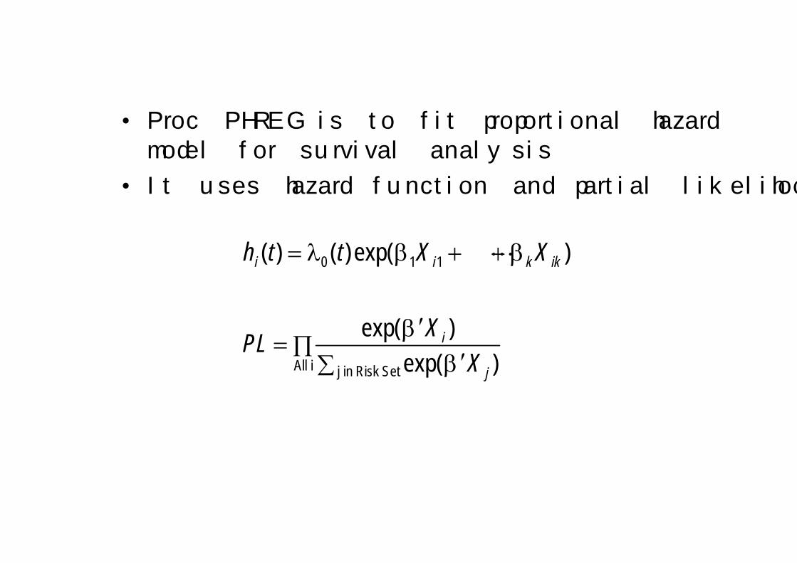
• Proc PHREG is to fit proportional hazard model for survival analysis
• It uses hazard function and partial likelihood
λ β β
ββ
∏∑
= + +
′=
′
0 1 1
All i j in Risk Set
( ) ( )exp( )
exp( )exp( )
i i k ik
i
j
h t t X X
XPLX
λ β β
ββ
∏∑
= + +
′=
′
0 1 1
All i j in Risk Set
( ) ( )exp( )
exp( )exp( )
i i k ik
i
j
h t t X X
XPLX
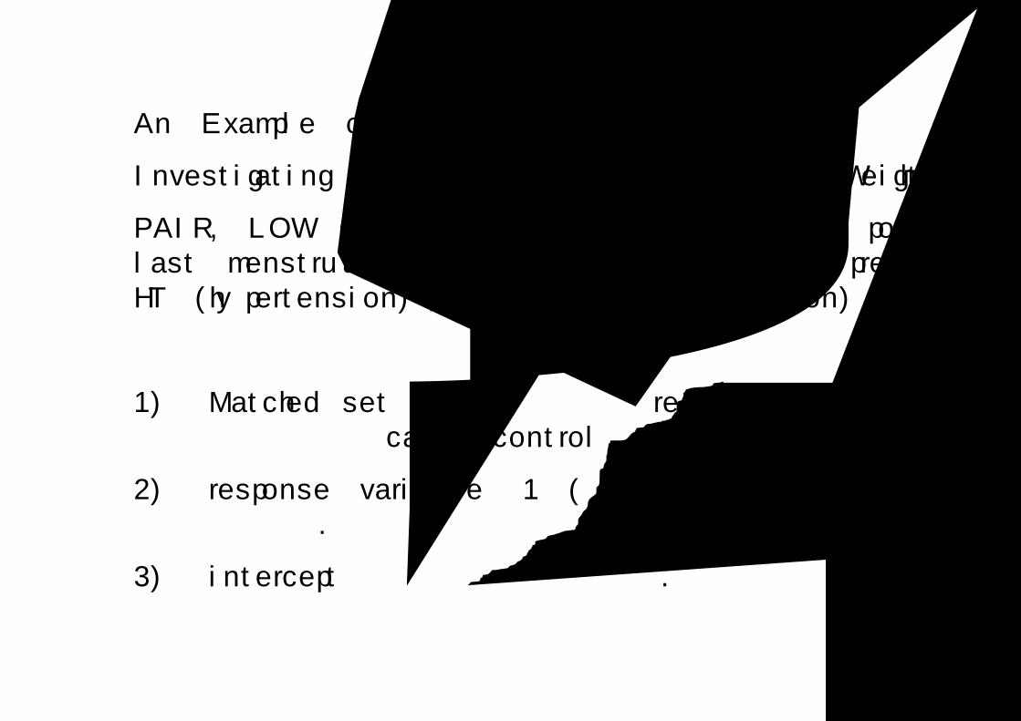
An Example of 1:1 matched Data
Investigating Risk factors for Low Birth Weight
PAIR, LOW (<2500g), AGE, LWT (weight in pounds at last menstrual period), PTD (history of premature labor), HT (hypertension), UI (uterine irritation)
1) Matched set 하나 마다 하나의 record (한 관측치)를 만들고 독립변수들은 case와 control의 차이들을 계산한다.
2) response variable은 1 (혹은 하나의 상수)의 값을 가지도록 고정한다.
3) intercept가 포함되지 않도록 한다.
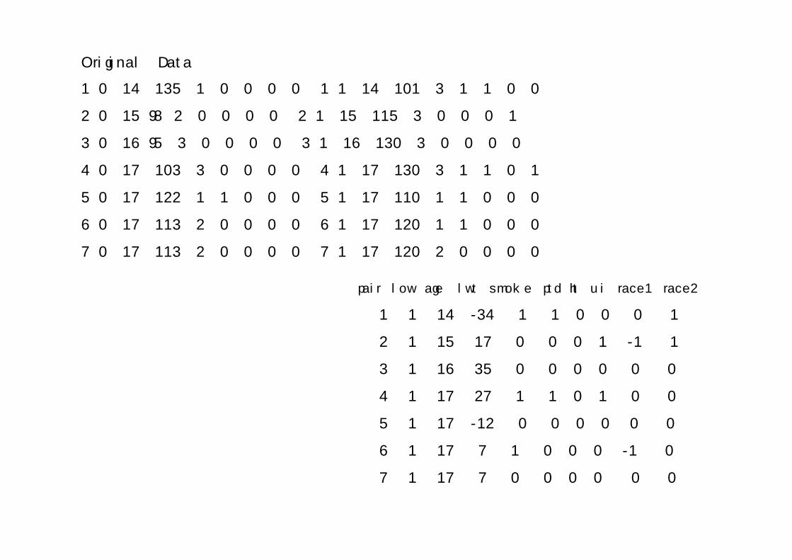
Original Data
1 0 14 135 1 0 0 0 0 1 1 14 101 3 1 1 0 0
2 0 15 98 2 0 0 0 0 2 1 15 115 3 0 0 0 1
3 0 16 95 3 0 0 0 0 3 1 16 130 3 0 0 0 0
4 0 17 103 3 0 0 0 0 4 1 17 130 3 1 1 0 1
5 0 17 122 1 1 0 0 0 5 1 17 110 1 1 0 0 0
6 0 17 113 2 0 0 0 0 6 1 17 120 1 1 0 0 0
7 0 17 113 2 0 0 0 0 7 1 17 120 2 0 0 0 0
pair low age lwt smoke ptd ht ui race1 race2
1 1 14 -34 1 1 0 0 0 1
2 1 15 17 0 0 0 1 -1 1
3 1 16 35 0 0 0 0 0 0
4 1 17 27 1 1 0 1 0 0
5 1 17 -12 0 0 0 0 0 0
6 1 17 7 1 0 0 0 -1 0
7 1 17 7 0 0 0 0 0 0
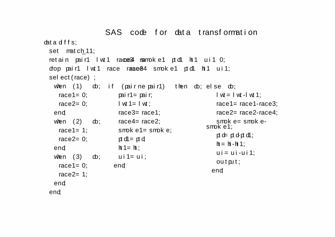
SAS code for data transformationdata diffs;
set match_11;
retain pair1 lwt1 race3 race4 smoke1 ptd1 ht1 ui1 0;
drop pair1 lwt1 race race3 race4 smoke1 ptd1 ht1 ui1;
select(race);
when (1) do;
race1=0;
race2=0;
end;
when (2) do;
race1=1;
race2=0;
end;
when (3) do;
race1=0;
race2=1;
end;
end;
if (pair ne pair1) then do;
pair1=pair;
lwt1=lwt;
race3=race1;
race4=race2;
smoke1=smoke;
ptd1=ptd;
ht1=ht;
ui1=ui;
end;
else do;
lwt=lwt-lwt1;
race1=race1-race3;
race2=race2-race4;
smoke=smoke-smoke1;
ptd=ptd-ptd1;
ht=ht-ht1;
ui=ui-ui1;
output;
end;
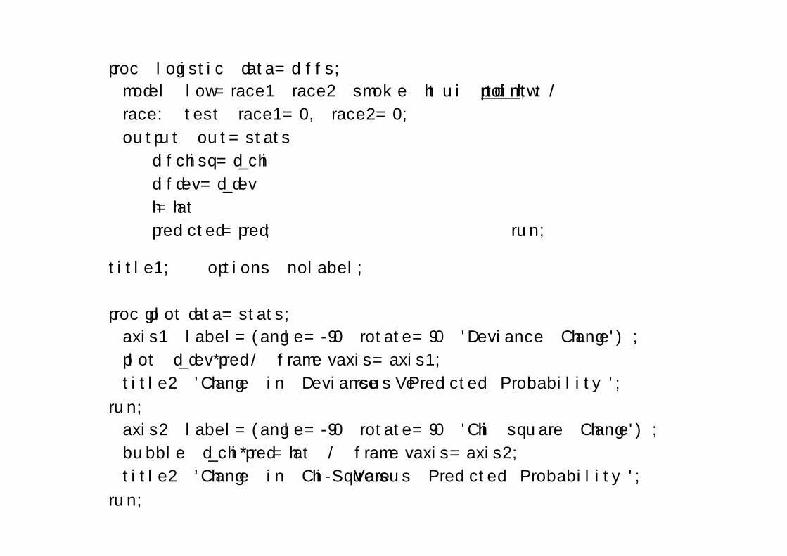
proc logistic data=diffs;
model low=race1 race2 smoke ht ui ptd lwt / noint;
race: test race1=0, race2=0;
output out=stats
difchisq=d_chi
difdev=d_dev
h=hat
predicted=pred; run;
title1; options nolabel;
proc gplot data=stats;
axis1 label=(angle=-90 rotate=90 'Deviance Change');
plot d_dev*pred / frame vaxis=axis1;
title2 'Change in Deviance Versus Predicted Probability';
run;
axis2 label=(angle=-90 rotate=90 'Chi square Change');
bubble d_chi*pred=hat / frame vaxis=axis2;
title2 'Change in Chi-Square Versus Predicted Probability';
run;
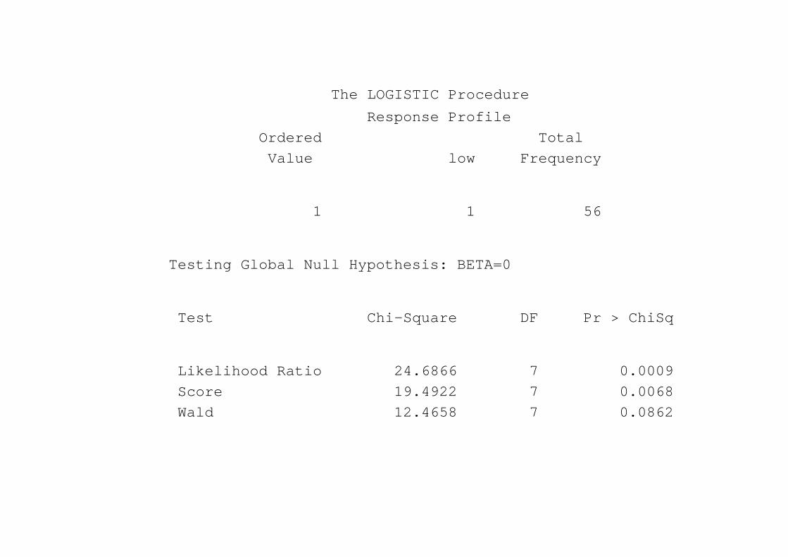
The LOGISTIC Procedure
Response Profile Ordered Total Value low Frequency
1 1 56
Testing Global Null Hypothesis: BETA=0
Test Chi-Square DF Pr > ChiSq
Likelihood Ratio 24.6866 7 0.0009 Score 19.4922 7 0.0068Wald 12.4658 7 0.0862
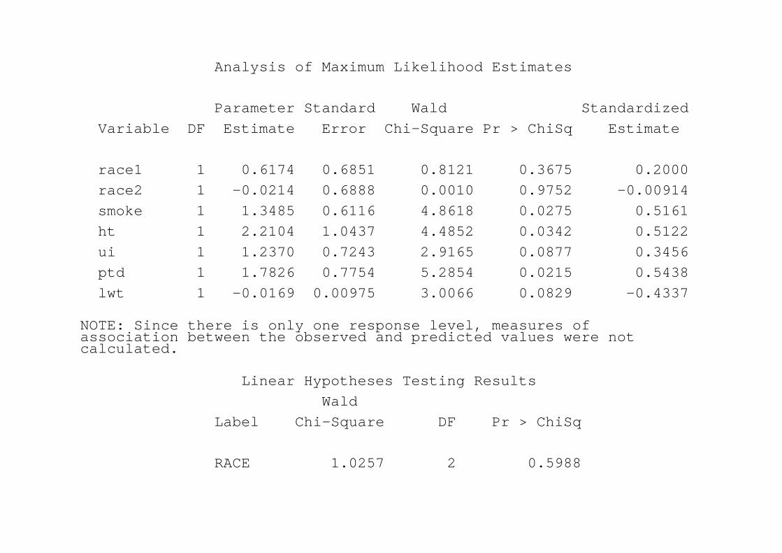
Analysis of Maximum Likelihood Estimates
Parameter Standard Wald Standardized Variable DF Estimate Error Chi-Square Pr > ChiSq Estimate
race1 1 0.6174 0.6851 0.8121 0.3675 0.2000 race2 1 -0.0214 0.6888 0.0010 0.9752 -0.00914 smoke 1 1.3485 0.6116 4.8618 0.0275 0.5161 ht 1 2.2104 1.0437 4.4852 0.0342 0.5122ui 1 1.2370 0.7243 2.9165 0.0877 0.3456ptd 1 1.7826 0.7754 5.2854 0.0215 0.5438lwt 1 -0.0169 0.00975 3.0066 0.0829 -0.4337
NOTE: Since there is only one response level, measures of association between the observed and predicted values were not calculated.
Linear Hypotheses Testing ResultsWald
Label Chi-Square DF Pr > ChiSq
RACE 1.0257 2 0.5988
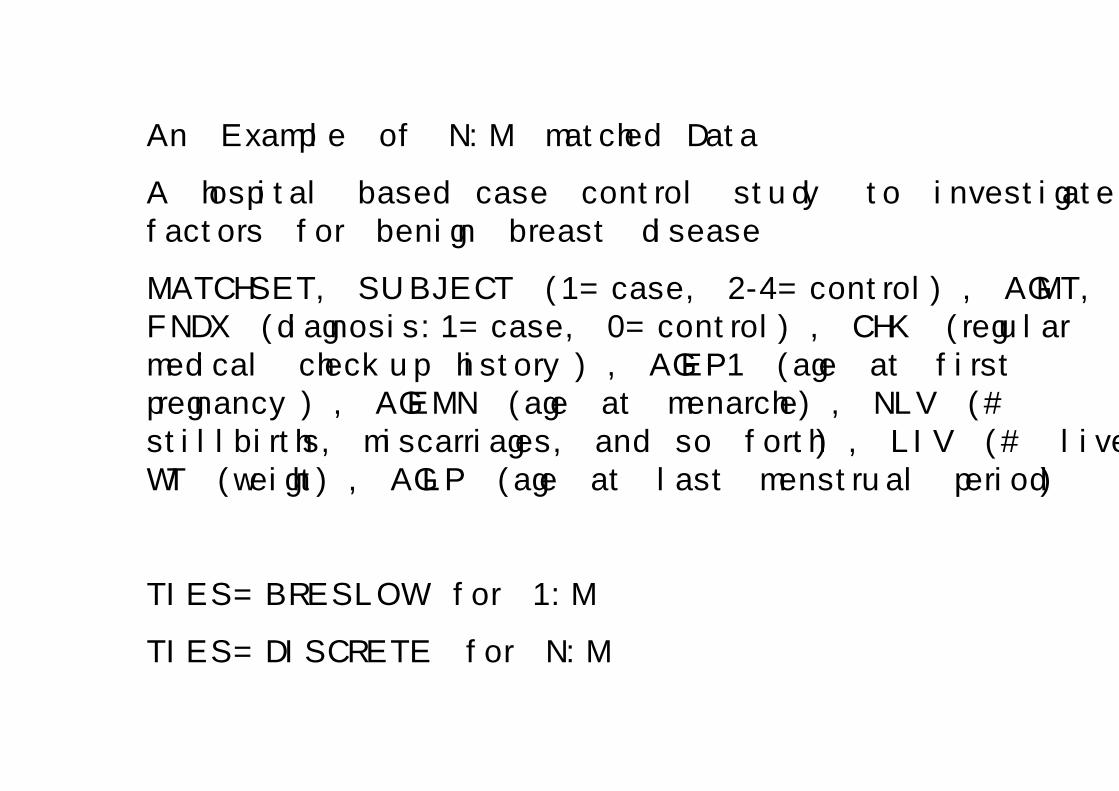
An Example of N:M matched Data
A hospital based case control study to investigate risk factors for benign breast disease
MATCHSET, SUBJECT (1=case, 2-4=control), AGMT, FNDX (diagnosis:1=case, 0=control), CHK (regular medical checkup history), AGEP1 (age at first pregnancy), AGEMN (age at menarche), NLV (# stillbirths, miscarriages, and so forth), LIV (# live birth), WT (weight), AGLP (age at last menstrual period)
TIES=BRESLOW for 1:M
TIES=DISCRETE for N:M
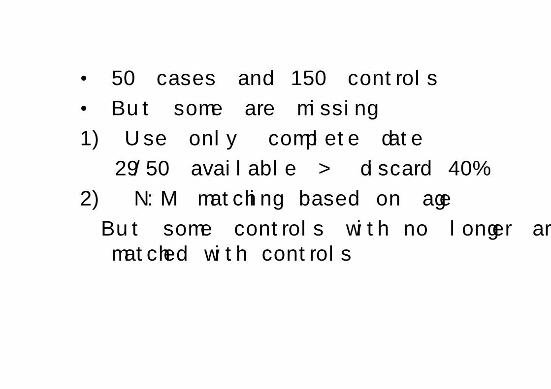
• 50 cases and 150 controls
• But some are missing
1) Use only complete date
29/50 available > discard 40%
2) N:M matching based on age
But some controls with no longer are matched with controls
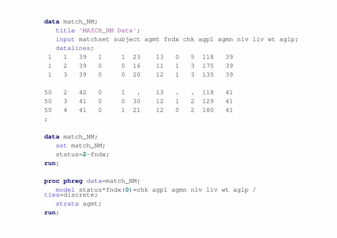
data match_NM;title 'MATCH_NM Data';input matchset subject agmt fndx chk agp1 agmn nlv liv wt aglp;datalines;
1 1 39 1 1 23 13 0 5 118 391 2 39 0 0 16 11 1 3 175 391 3 39 0 0 20 12 1 3 135 39
50 2 42 0 1 . 13 . . 118 4150 3 41 0 0 30 12 1 2 129 4150 4 41 0 1 21 12 0 2 180 41;
data match_NM;set match_NM;status=2-fndx;
run;
proc phreg data=match_NM;model status*fndx(0)=chk agp1 agmn nlv liv wt aglp /
ties=discrete;strata agmt;
run;
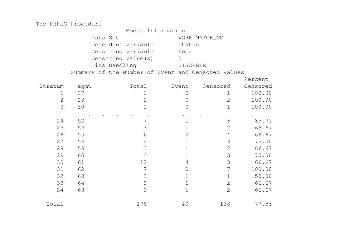
The PHREG ProcedureModel Information
Data Set WORK.MATCH_NMDependent Variable statusCensoring Variable fndxCensoring Value(s) 0Ties Handling DISCRETE
Summary of the Number of Event and Censored ValuesPercent
Stratum agmt Total Event Censored Censored1 27 1 0 1 100.002 28 2 0 2 100.003 30 1 0 1 100.00
. . . . . . . . 24 52 7 1 6 85.7125 53 3 1 2 66.6726 55 6 2 4 66.6727 56 4 1 3 75.0028 58 3 1 2 66.6729 60 4 1 3 75.0030 61 12 4 8 66.6731 62 7 0 7 100.0032 63 2 1 1 50.0033 64 3 1 2 66.6734 68 3 1 2 66.67
-------------------------------------------------------------------Total 178 40 138 77.53
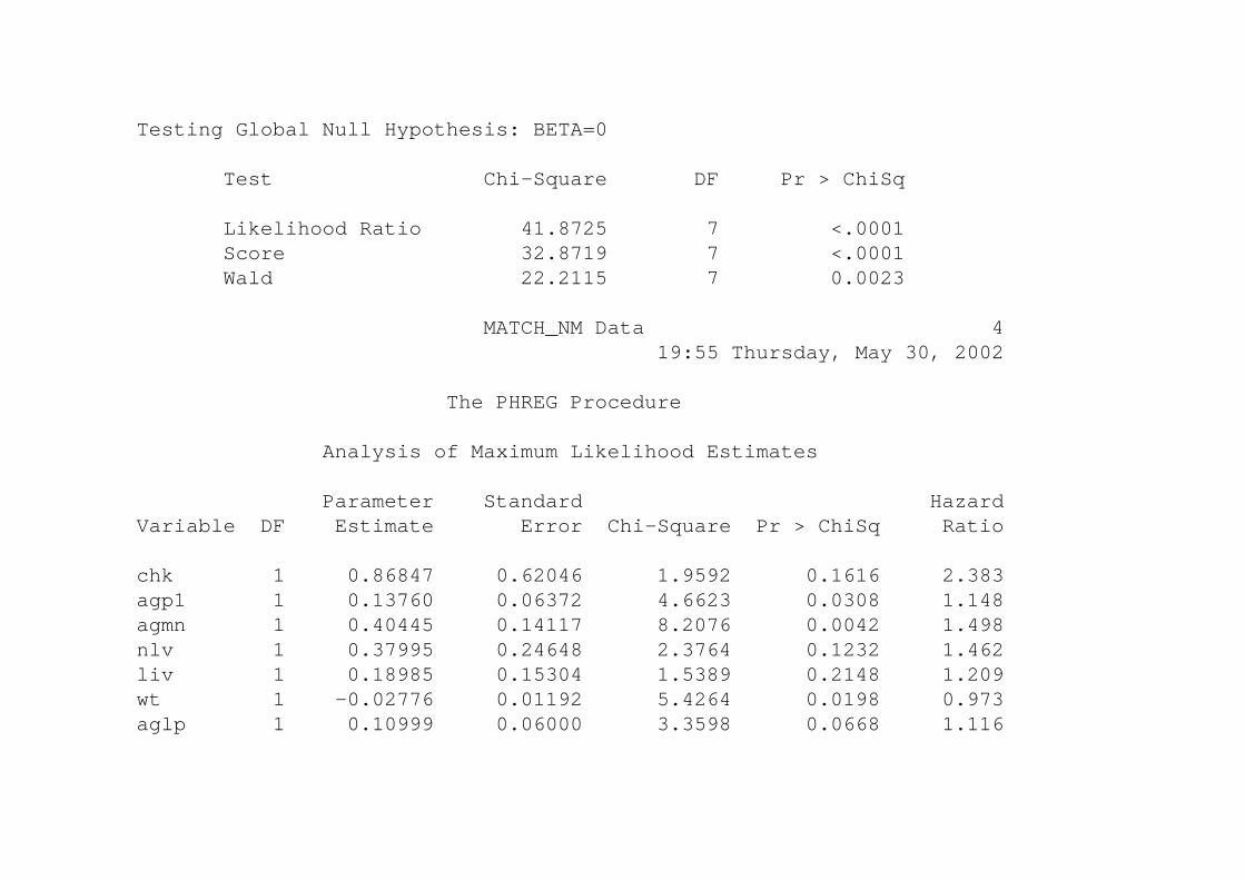
Testing Global Null Hypothesis: BETA=0
Test Chi-Square DF Pr > ChiSq
Likelihood Ratio 41.8725 7 <.0001Score 32.8719 7 <.0001Wald 22.2115 7 0.0023
MATCH_NM Data 419:55 Thursday, May 30, 2002
The PHREG Procedure
Analysis of Maximum Likelihood Estimates
Parameter Standard HazardVariable DF Estimate Error Chi-Square Pr > ChiSq Ratio
chk 1 0.86847 0.62046 1.9592 0.1616 2.383agp1 1 0.13760 0.06372 4.6623 0.0308 1.148agmn 1 0.40445 0.14117 8.2076 0.0042 1.498nlv 1 0.37995 0.24648 2.3764 0.1232 1.462liv 1 0.18985 0.15304 1.5389 0.2148 1.209wt 1 -0.02776 0.01192 5.4264 0.0198 0.973aglp 1 0.10999 0.06000 3.3598 0.0668 1.116
• Crossover study is an application of conditional logistic regression analysis in the clinical trials
• Case-crossover design is a relatively new methodology in epidemiology.
• Some case-crossover studies in occupational and environmental epidemiology/medicine.
• Simulation studies to understand statistical properties
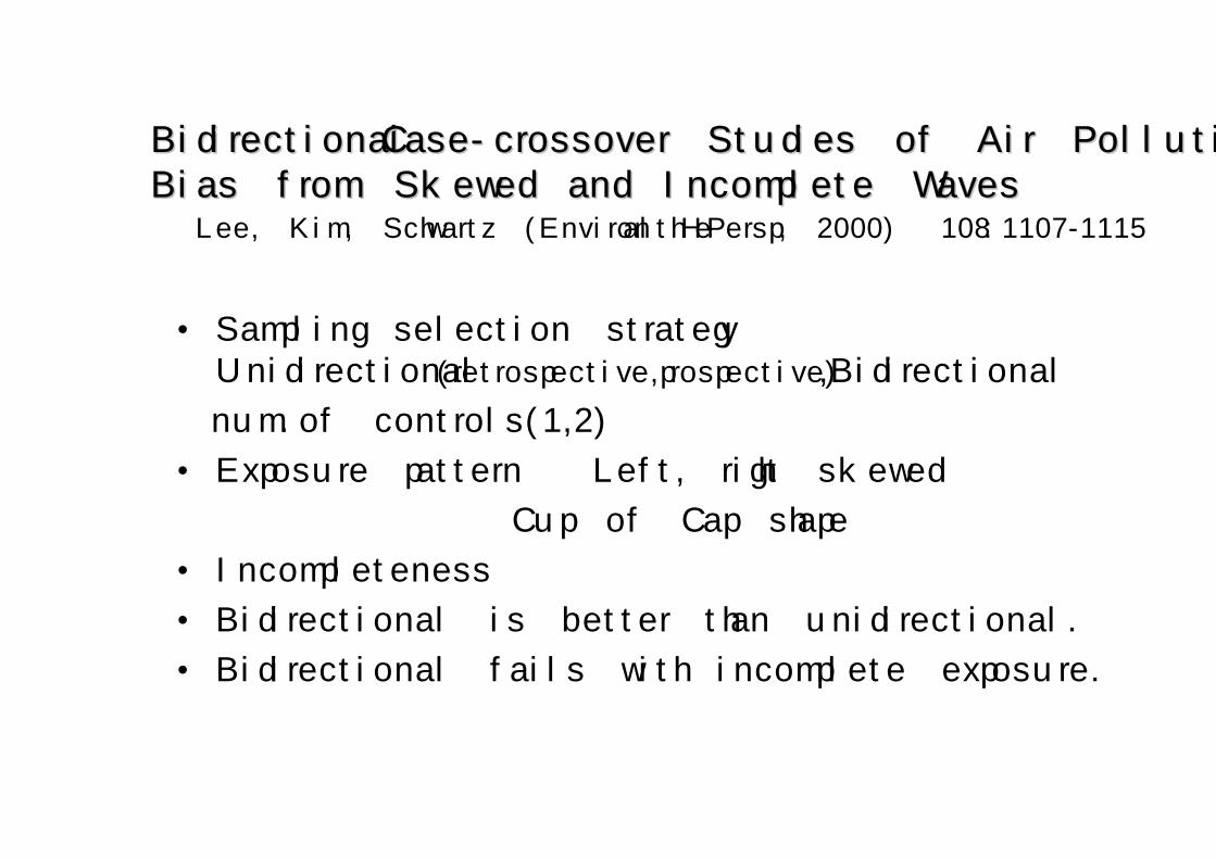
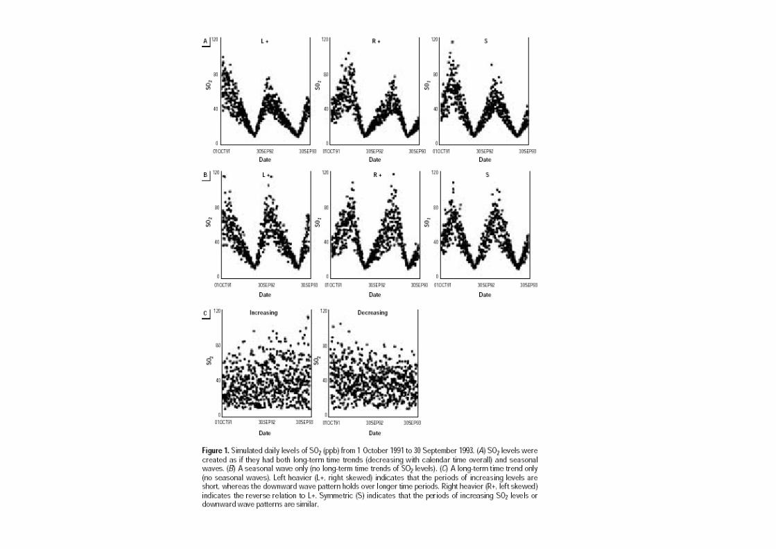
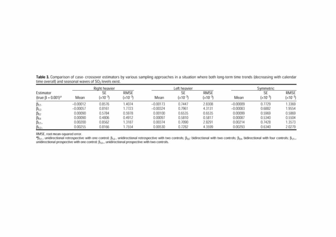
BidirectionalBidirectional CaseCase--crossover Studies of Air Pollution:crossover Studies of Air Pollution:Bias from Skewed and Incomplete WavesBias from Skewed and Incomplete Waves
Lee, Kim, Schwartz (Environ Health Persp, 2000) 108:1107-1115
• Sampling selection strategy Unidirectional(retrospective,prospective),Bidirectional
num.of controls(1,2)
• Exposure pattern Left, right skewed
Cup of Cap shape
• Incompleteness
• Bidirectional is better than unidirectional.
• Bidirectional fails with incomplete exposure.
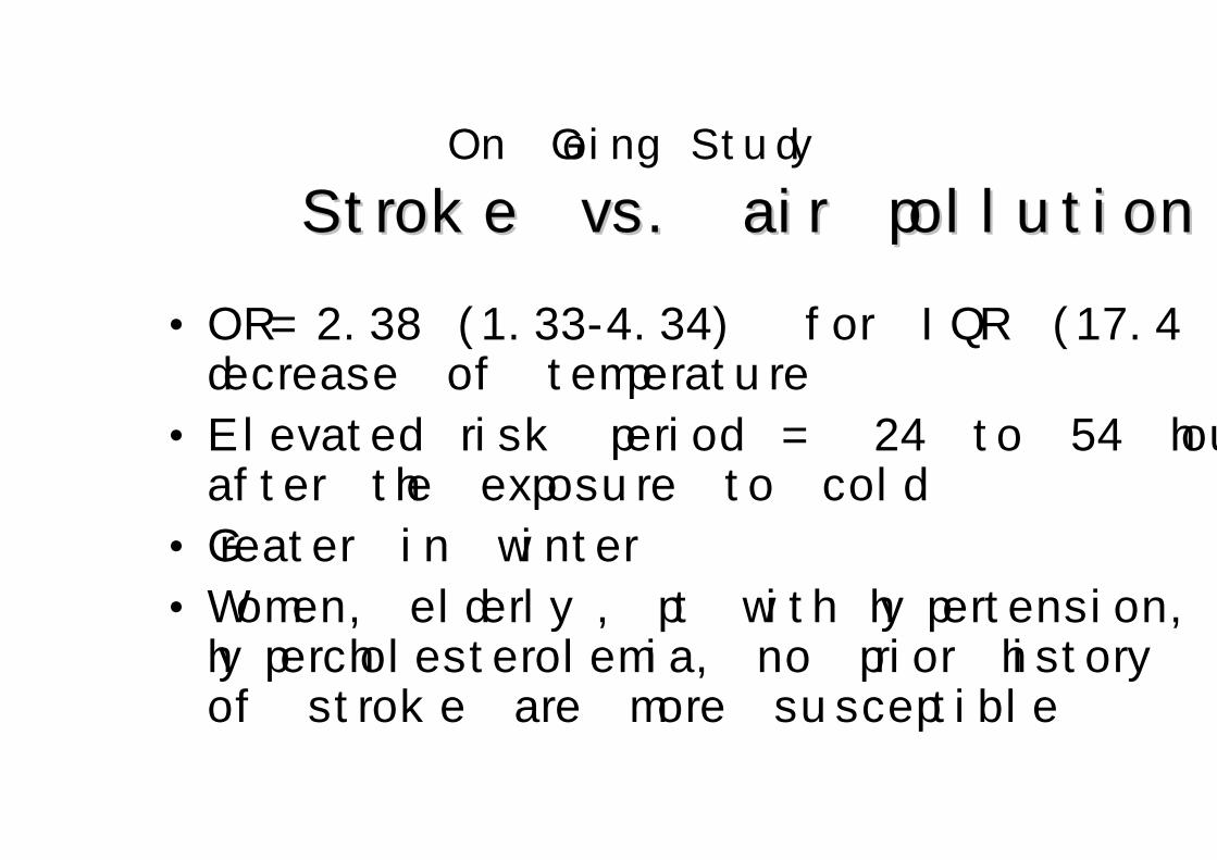
On Going Study
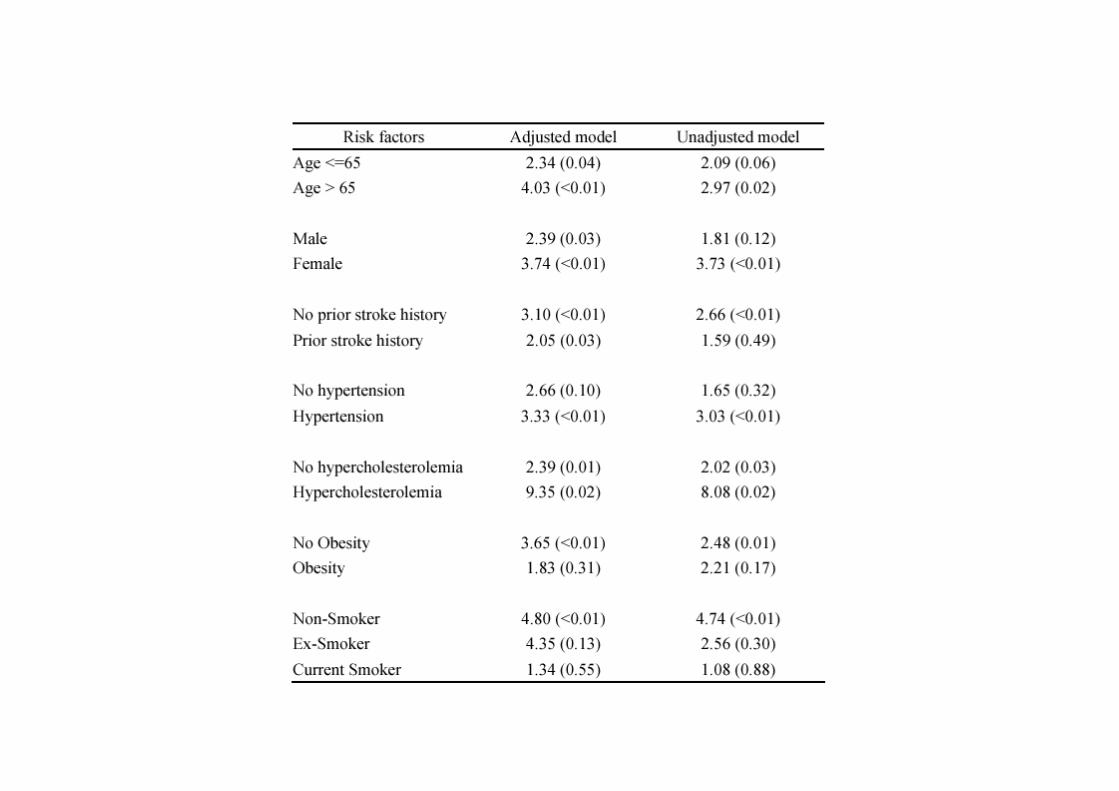
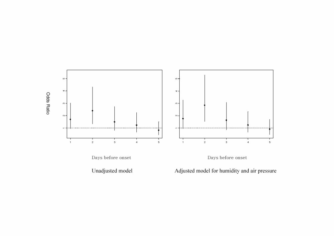
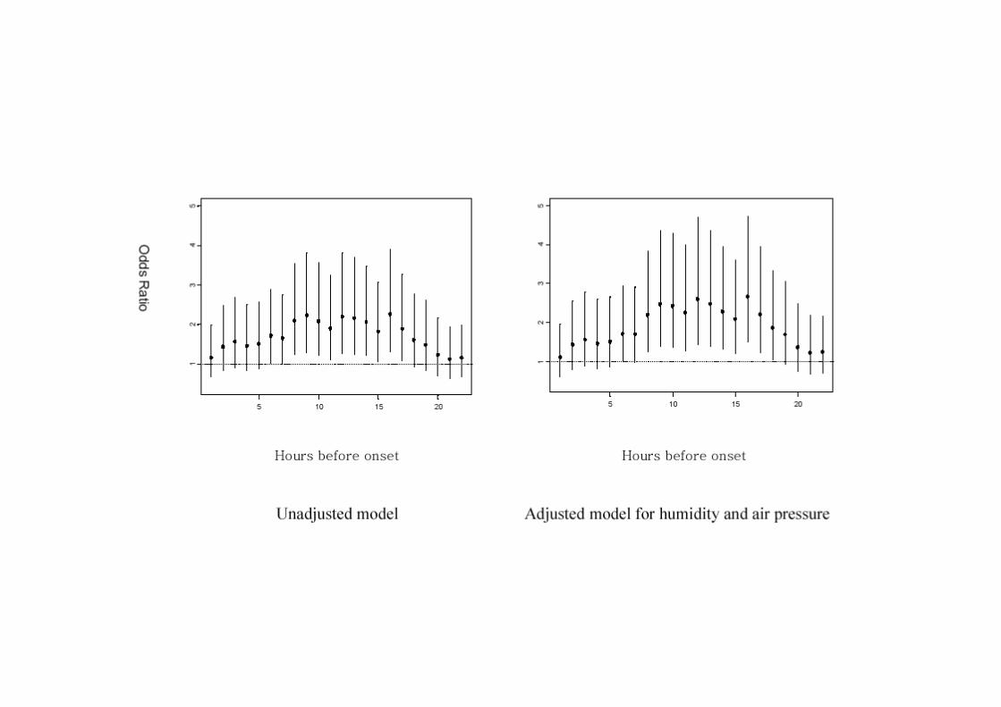
Stroke vs. air pollutionStroke vs. air pollution
• OR=2.38 (1.33-4.34) for IQR (17.4 C) decrease of temperature
• Elevated risk period = 24 to 54 hours after the exposure to cold
• Greater in winter
• Women, elderly, pt with hypertension, hypercholesterolemia, no prior history of stroke are more susceptible