introduction to data analysis
DESCRIPTION
Introduction to Data Analysis. Probability Confidence Intervals. Today’s lecture. Some stuff on probability Confidence intervals (A&F 5). Standard error (part 2) and efficiency. Confidence intervals for means. Confidence intervals for proportions. Last week’s aide memoire. - PowerPoint PPT PresentationTRANSCRIPT
Introduction to Data Analysis
Probability
Confidence Intervals
2
Today’s lecture
Some stuff on probability
Confidence intervals (A&F 5). Standard error (part 2) and efficiency. Confidence intervals for means. Confidence intervals for proportions.

3
Last week’s aide memoire Population distribution
We don’t know this, but we want to know about it. In particular we normally want to know the mean.
Sample distribution We know this, and calculate the statistics such as the sample mean
and the sample standard deviation from it.
Sampling distribution This describes the variability in value of the sample means
amongst all the possible samples of a certain size. We can work this out from information about the sample
distribution and the fact that the sampling distribution is normal if sample size is large (ish).

4
Random Variables
Flip a coin. Will it be heads or tails? The outcome of a single event is random, or
unpredictable What if we flip a coin 10 times? How many
will be heads and how many will be tails? Over time, patterns emerge from seemingly
random events. These allow us to make probability statements.

5
Heads or Tails?
A coin toss is a random event [H or T] unpredictable on each toss but a stable pattern emerges of 50:50 after many repetitions.
The French naturalist, Buffon (1707-1788) tossed a coin 4040 times; resulting in 2048 heads for a relative frequency of 2048 /4040 = .5069
6
Heads or Tails?
The English mathematician John Kerrich, while imprisoned by Germans in WWII, tossed a coin 5,000 times, with result 2534 heads . What is the Relative Frequency?
2,534 / 5,000 = .5068

7

8
Heads or tails?
A computer simulation of 10,000 coin flips yields 5040 heads. What is the relative frequency of heads?
5040 / 10,000 = .5040

9
Each of the tests is the result of a sample of fair coin tosses.
Sample outcomes vary. • Different samples produce different results.
True, but the law of large numbers tells us that the greater the number of repetitions the closer the outcomes come to the true probability, here .5.
A single event may be unpredictable but the relative frequency of these events is lawful over an infinite number of trials\repetitions.

10
Random Variables "X" denotes a random variable. It is the outcome of a
sample of trials. “X,” some event, is unpredictable in the short run but
lawful over the long run. This “Randomness” is not necessarily unpredictable.
Over the long run X becomes probabilistically predictable.
We can never observe the "real" probability, since the "true" probability is a concept based on an infinite number of repetitions/trials. It is an "idealized" version of events

11
To figure the odds of some event occurring you need 2 pieces of information:
1. A list of all the possibilities – all the possible outcomes (sample space)
2. The number of ways to get the outcome of interest (relative to the number of possible outcomes).
12
Take a single Dice Roll
Assuming an evenly-weighted 6-sided dice, what are the odds of rolling a 3?
How do you know?6 possible outcomes (equally likely)1 way to get a 3p(Roll=3) = 1 / 6

13
What are the chances of rolling numbers that add up to “4” when rolling two six-sided dice?
What do we need to know?All Possible Outcomes from rolling two diceOutcomes that would add up to 4

14
How Many Ways can the Two Dice Fall?
Let’s say the dice are different colors (helps us keep track.
The White Dice could come out as:
We know how to figure out probabilities here, butWhat about the other dice?
15
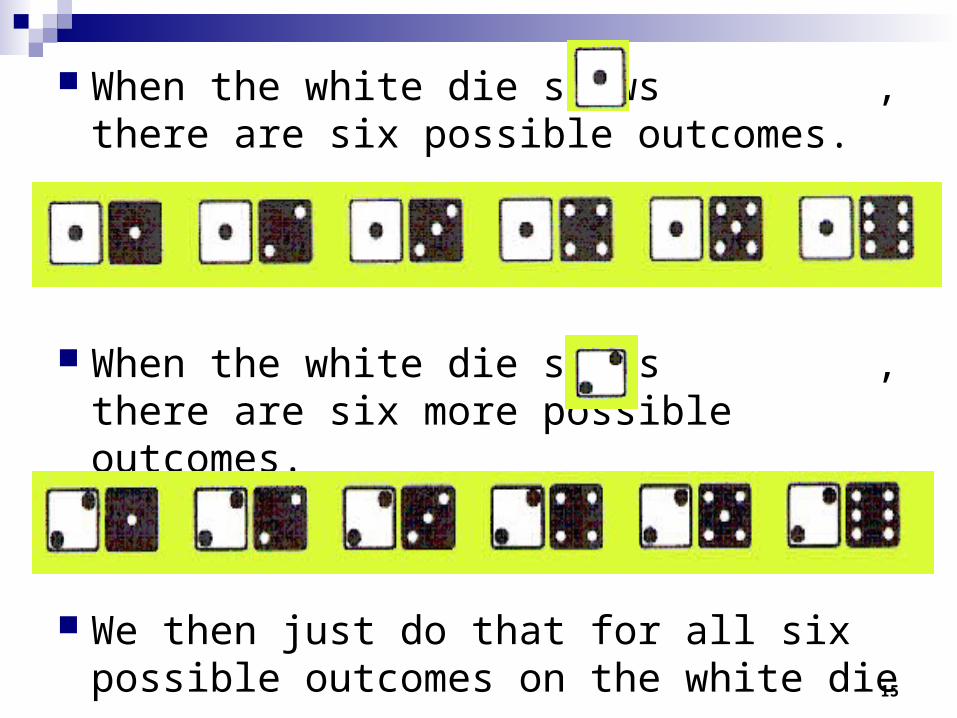
When the white die shows , there are six possible outcomes.
When the white die shows , there are six more possible outcomes.
We then just do that for all six possible outcomes on the white die

16

17
Remember the Question: What is the probability of Rolling numbers that sum to 4?
What do we need to know? All Possible Outcomes from rolling two dice
(36--Check Previous Slide) How many outcomes would add up to 4?
Our Probability is 3/36 = .08333
18
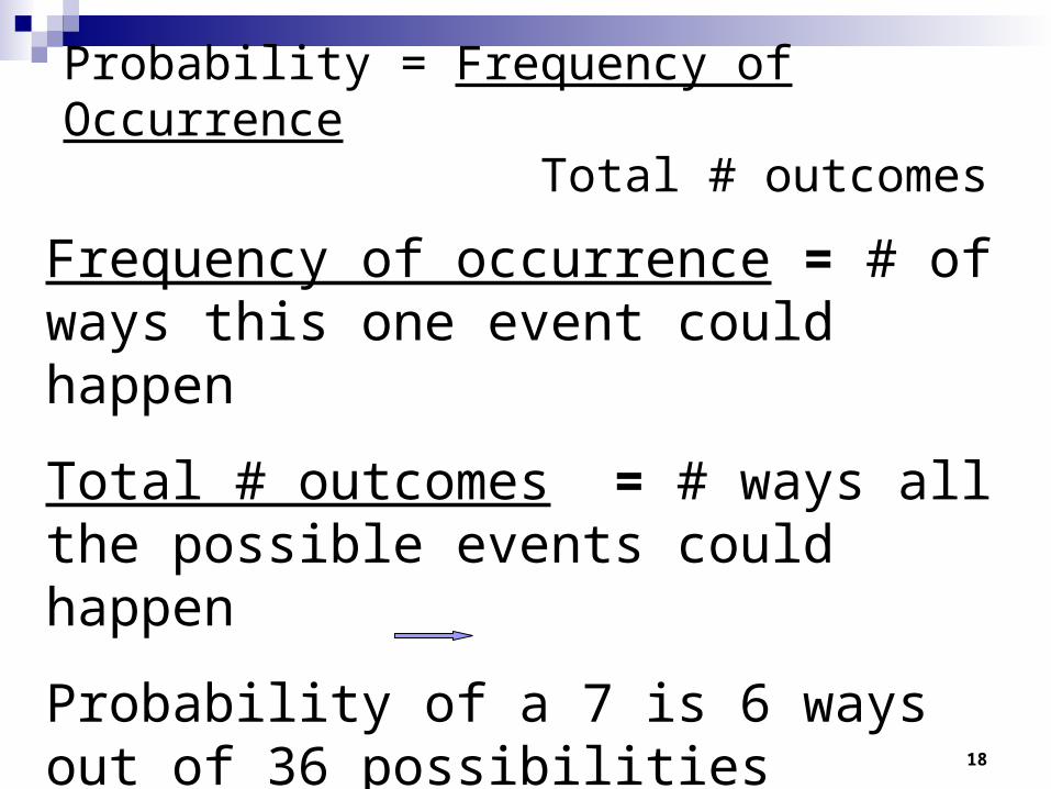
Probability = Frequency of Occurrence Total # outcomes
Frequency of occurrence = # of ways this one event could happen
Total # outcomes = # ways all the possible events could happen
Probability of a 7 is 6 ways out of 36 possibilities p=.166
19
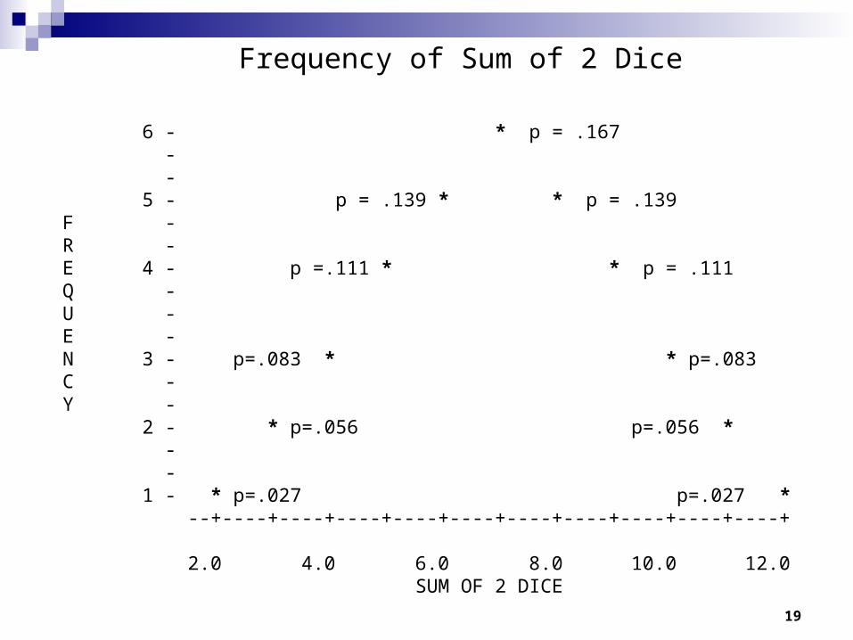
Frequency of Sum of 2 Dice 6 - * p = .167 - - 5 - p = .139 * * p = .139 F - R - E 4 - p =.111 * * p = .111 Q - U - E - N 3 - p=.083 * * p=.083 C - Y - 2 - * p=.056 p=.056 * - - 1 - * p=.027 p=.027 * --+----+----+----+----+----+----+----+----+----+----+ 2.0 4.0 6.0 8.0 10.0 12.0 SUM OF 2 DICE
20
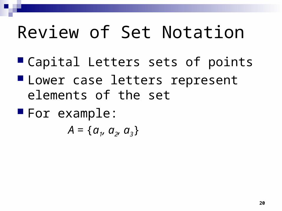
Review of Set Notation
Capital Letters sets of points Lower case letters represent elements of the
set For example:
A = {a1, a2, a3}
21
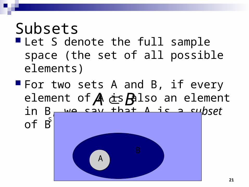
Let S denote the full sample space (the set of all possible elements)
For two sets A and B, if every element of A is also an element in B, we say that A is a subset of B A B
S
BA
Subsets

22
Union
The union of two arbitrary sets of points is the set of all points that are in at least one of the sets A B
A
S
B

23
Intersection The intersection of two arbitrary sets of points
is the set of all points that are in both of the sets
A B

24
Mutual Exclusivity
Two events are said to be disjoint or mutually exclusive if none of the elements in set A appear in set B.

25
Independence We will give a more rigorous definition later,
but… Two events are independent if the occurrence of A
is unaffected by the occurrence or nonoccurrence of B.
Example: You flip a coin—what is the probability of heads?
You flip it 10 times, getting heads each time. What is the probability of getting heads again?

26
Axioms for Probabilities
The conventional rules for probabilities are named the Kolmogorov Axioms. They are:1.
2.
3. If A1, A2, A3, … are pairwise mutually exclusive events in S, then:
( ) 0P A ( ) 1P S
1 2 3( ) ( )iP A A A P A

27
Rules for Calculating Probabilities
Simple Additive rule for disjoint events a.k.a. the “or” rule
( ) ( ) ( )P A B P A P B
A
S
B
28
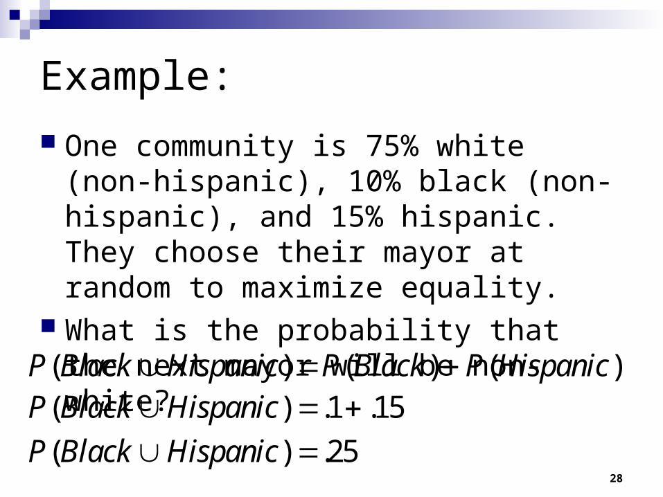
Example:
One community is 75% white (non-hispanic), 10% black (non-hispanic), and 15% hispanic. They choose their mayor at random to maximize equality.
What is the probability that the next mayor will be non-white?
( ) ( ) ( )P Black Hispanic P Black P Hispanic ( ) .1 .15P Black Hispanic ( ) .25P Black Hispanic

29
Rules for Calculating Probabilities
Simple Multiplicative rule for independent events a.k.a. the “and” rule
( ) ( )* ( )P A B P A P B

30
Example:
Suppose in that same mythical community (75% white, 10% black, 15% Hispanic) there was an even division of males and females. What is the probability of a white male mayor?
( ) ( )* ( )P White Male P White P Male ( ) (.75)*(.5)P White Male ( ) .375P White Male
31
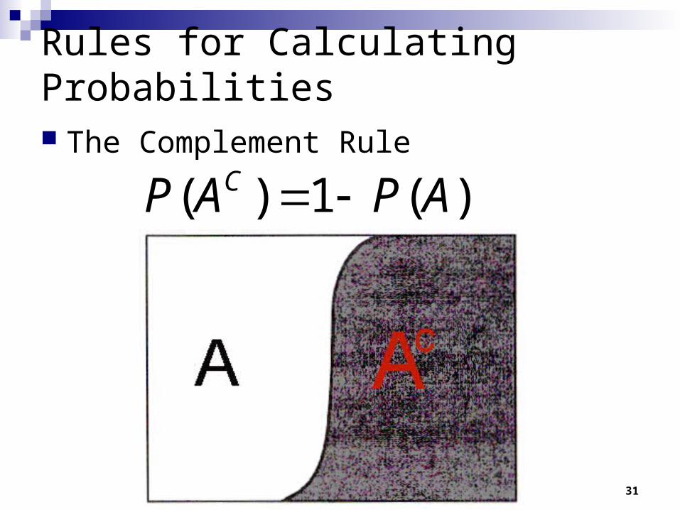
Rules for Calculating Probabilities
The Complement Rule
( ) 1 ( )CP A P A

32
Rules for Calculating Probabilities
Additive rule for events that are not mutually exclusive events
( ) ( ) ( ) ( )P A B P A P B P A B
33
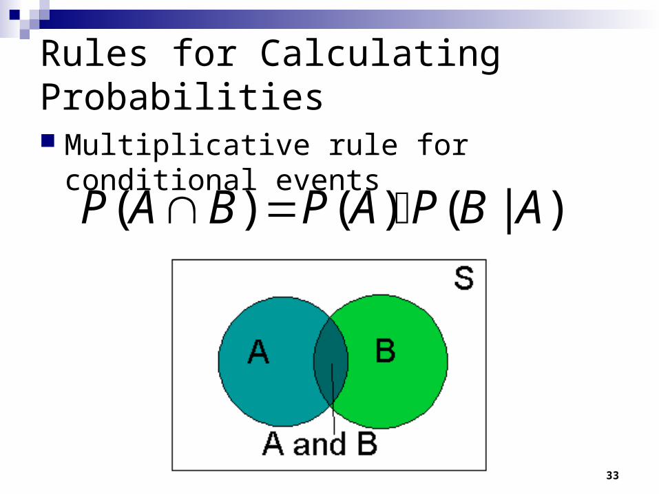
Rules for Calculating Probabilities
Multiplicative rule for conditional events
( ) ( ) ( | )P A B P A P B A

34
But wait…
Now we know the rules for manipulating probabilities mathematically, but to get them, we need to calculate the sample space and the number of ways to get the outcome

35
Tools for Counting Sample Spaces
Listing The mn rule Permutations (Pn
r)
Combinations (Cnr)
36
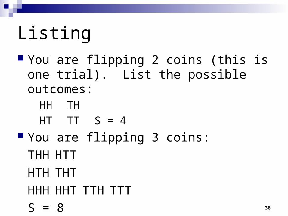
Listing You are flipping 2 coins (this is one trial). List
the possible outcomes:HH TH
HT TT S = 4 You are flipping 3 coins:
THH HTT
HTH THT
HHH HHT TTH TTT
S = 8

37
Listing
AdvantagesIntuitiveEasy (with a small sample space)
DisadvantagesHard to do with a large sample space

38
The mn rule Think of the coin example—there are 2
possible outcomes for each coin, and 2 coins. Thus, there are 2 * 2 = 4 possible outcomes
Think of the dice example—there are 6 possible outcomes for each dice, and 2 dice. Thus, there are 6 * 6 = 36 possible outcomes

39
The mnp rule ? It works for more than 2 dice/coins or
whatever too. Consider the 3 coin flips:2 * 2 * 2 = 23 = 8
This can be thought of as successive applications of the mn rule. First, you get the combinations of 2 coin flips
mn = 2 * 2 = 4 Then you get the combination of that sample
space with the 3rd coin(mn)*p = 4 * 2 = 8
40
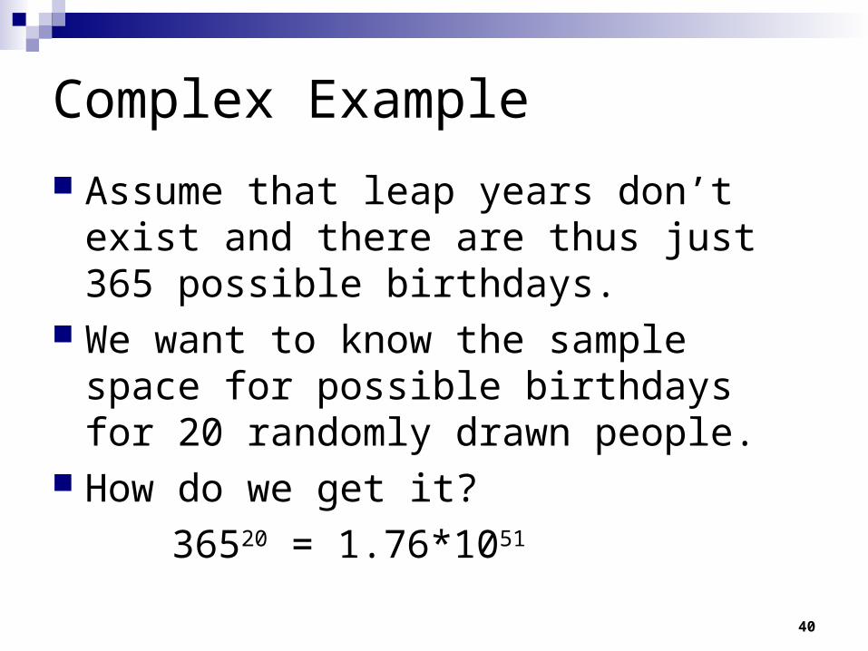
Complex Example
Assume that leap years don’t exist and there are thus just 365 possible birthdays.
We want to know the sample space for possible birthdays for 20 randomly drawn people.
How do we get it?
36520 = 1.76*1051

41
Complex Example
Assuming that each birthday is equally likely, what is the probability of everyone having a January 1 Birthday?
What is the probability that everyone has the same birthday?
20
1
365
20 19
365 1
365 365
42
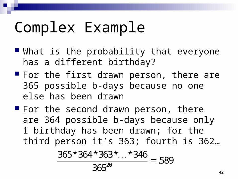
Complex Example
What is the probability that everyone has a different birthday?
For the first drawn person, there are 365 possible b-days because no one else has been drawn
For the second drawn person, there are 364 possible b-days because only 1 birthday has been drawn; for the third person it’s 363; fourth is 362…
20
365*364*363* *346.589
365
43
Permutations In some situations, we will be concerned with
the order in which sequences occur. An ordered arrangement of r objects is called a
permutation The number of possible permutations is denoted
as Our proof is based on our extension of the mn
rule in the last problem…
nrP
nrP

44
We are interested in filling r positions with n distinct objects—no repeated values (selecting 20 people with 365 possible birthdays)
Permutations nrP
!
( 1)( 2)( 3)...( 1)!
nr
nP n n n n n r
n r

45
Permutation Example
Think of a chain lock with a combination that requires 4 digits (0-9)
How many possible combinations are there?
4 6 2 0
10
4
10! 10! 10*9*8*7*6*5*4*3*2*1
10 4 ! 6! 6*5*4*3*2*1P
10*9*8*7 5040

46
Combinations
In some situations, the ordering of the symbols in a set is unimportant—we only care what is included (not its position)
There will be fewer combinations than permutations—permutation counts HHT, HTH, and THH as being separate; combinations don’t consider the order, just the contents.
!
! ! !
nn rr
n P nC
r r r n r
47
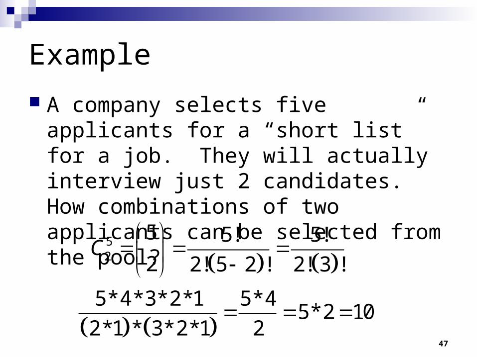
Example
A company selects five applicants for a “short list” for a job. They will actually interview just 2 candidates. How combinations of two applicants can be selected from the pool?
52
5 5! 5!
2 2! 5 2 ! 2! 3 !C
5*4*3*2*1 5*4
5*2 102*1 * 3*2*1 2
48
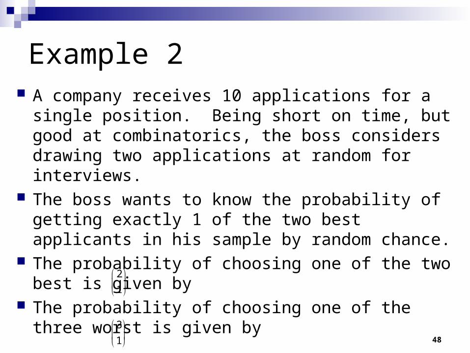
Example 2 A company receives 10 applications for a single
position. Being short on time, but good at combinatorics, the boss considers drawing two applications at random for interviews.
The boss wants to know the probability of getting exactly 1 of the two best applicants in his sample by random chance.
The probability of choosing one of the two best is given by
The probability of choosing one of the three worst is given by
2
1
3
1
49
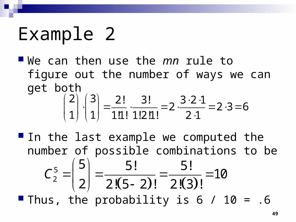
Example 2 We can then use the mn rule to figure out the
number of ways we can get both
In the last example we computed the number of possible combinations to be
Thus, the probability is 6 / 10 = .6
2 3 2! 3! 3 2 12 2 3 6
1 1 1!1! 1!2!1! 2 1
52
5 5! 5!10
2 2! 5 2 ! 2! 3 !C
50
Conditional Probability Under some circumstances the probability of
an event depends on another event. An unconditional probability asks what the
chances are of rain tomorrow (event A).
A conditional probability says, “Given that rained today (event B), what are the chances of rain tomorrow? (event A)”
P(A|B)
( )P A
51
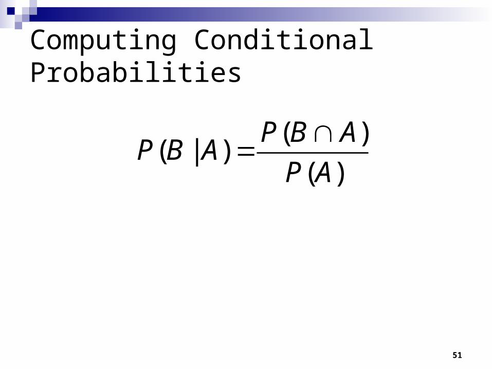
Computing Conditional Probabilities
( )( | )
( )
P B AP B A
P A

52
Independence
Two events are said to be independent if
Otherwise, the events are dependent
( | ) ( )P A B P A

53
Bayes’ Rule Suppose we knew P(B|A) but wanted to know
P(A|B)?
1
( ) ( | )( | )
( ) ( | )
j jj k
i ii
P B P A BP B A
P B P A B

54
Example Suppose you have been tested positive for a disease;
what is the probability that you actually have the disease? Suppose the probability of having the disease is .01. The test is 95% accurate, and you tested positive. Do you have the disease?
We know:The probability of anyone having the disease (.01)The probability of testing positive for the disease
conditional on having the disease (.95) We want to know the probability of having the
disease if you tested positive for it…

55
Bayes’ Rule( ) ( | )
( | )( ) ( | ) ( ) ( | )
P HaveIt P TestPos HaveItP HaveIt TestPos
P HaveIt P TestPos HaveIt P NoHaveIt P TestPos NoHaveIt
.01 .95( | )
.01 .95 .99 .05P HaveIt TestPos
.0095 .0095
( | ) .161.0095 .0495 .059
P HaveIt TestPos

56
What? .161? Why so low?
Out of 100 people who take this test, we expect only 1 would have the disease.
However, 5 people would test positive even if they didn’t have the disease.
Out of those 6 people, only 1 actually has the disease…
57
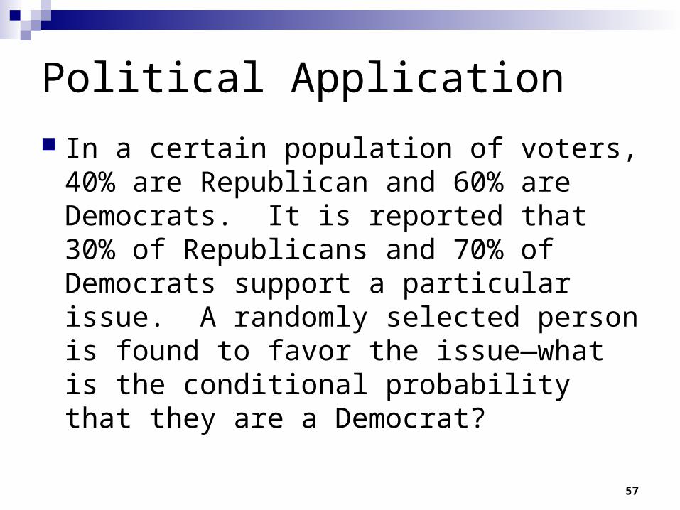
Political Application
In a certain population of voters, 40% are Republican and 60% are Democrats. It is reported that 30% of Republicans and 70% of Democrats support a particular issue. A randomly selected person is found to favor the issue—what is the conditional probability that they are a Democrat?

58
Work it out
We want to know P(Dem | F_issue)
( ) ( _ | )( | _ )
( ) ( _ | ) (Rep) ( _ | Rep)
P Dem P F issue DemP Dem F issue
P Dem P F issue Dem P P F issue
.6 .7( | _ )
.6 .7 .4 .3P Dem F issue
.42
( | _ ) .778.42 .12
P Dem F issue

59
Standard errors continued…
Last week we managed to work out some info about the distribution of sample means. If we have lots of samples then:
Mean of all the sample means = population mean. Shape of the distribution of sample means = normal. Standard error tells us how dispersed the distribution of
sample means is.
Put all these together, and we can finally work out how likely our sample mean is to be near the population mean.

60
Churchgoing example
Let’s take a less contrived example than my car managing to break any speed limits.
This week I’m interested in the average number of times a year people go to church (or synagogue, or whatever).
I take a sample of 100 people and record the number of times they went to church last year. Some went a lot but most went infrequently.
So, from that sample I get a sample mean and a sample standard deviation.

61
Church-going sample
0
10
20
30
40
50
60
0 10 20 30 40 50 60
Number of times per year
Freq
uenc
y
Sample mean = 8.5
Sample s.d. = 20

62
Standard error Since we know the s.d. and mean of the sample, we can
calculate the standard error.
Because we know the standard error and the fact that the sampling distribution is normal, we are able to calculate how ‘likely’ it is that a specific range around our estimate contains the population mean.
We can calculate what’s called a confidence interval.
63
Confidence intervals (1)
A confidence interval for an estimate is a range of numbers within which the parameter is ‘likely’ to fall.
Remember a parameter is something about the population, like the population mean.
We can use the standard error (and the fact that the sampling distribution is normal) to produce such a range.

64
Confidence intervals (2)
k is chosen to determine what is meant by ‘likely’ to contain the actual value of the population mean.
We want to pick a k that is meaningful to us. … and is not so large that the interval is useless. … but not so small that the interval is very unlikely to
contain the true population value.
)error standard(estimate k

65
Confidence intervals (3)
To return to our example, we have: An estimate of the population mean (the
mean number of days of church attendance) which is the sample mean (8 ½ days).
A standard error (2 days) which allows us to put a range around our estimate.
)2(8.5 k

66
How do we pick k?
Imagine sampling repeatedly, and therefore getting lots of sample means.
Given what we know about the sampling distribution (i.e. it’s normal if n is large enough), we know what proportion of these sample means will fall within a certain number of standard errors of the actual population mean.

67
Confidence coefficient Call this proportion the confidence coefficient.
If we picked .95 then we know that if we repeatedly sampled the population, that interval around each of the sample means would include the true value 95% of the time.
The confidence coefficient is a number that is chosen by the researcher which is close to 1, like 0.95 or 0.99.
Since the sampling distribution is normal, we know the values of k that correspond to the probability of any proportion.
So we know that approximately 95% of confidence intervals that are 2 standard errors either side of the sample mean will include the population mean.
68
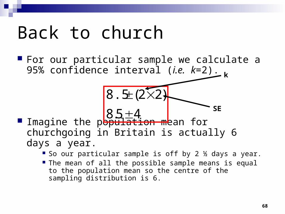
Back to church For our particular sample we calculate a 95%
confidence interval (i.e. k=2).
Imagine the population mean for churchgoing in Britain is actually 6 days a year.
So our particular sample is off by 2 ½ days a year. The mean of all the possible sample means is equal to the
population mean so the centre of the sampling distribution is 6.
45.8
)22(8.5
k
SE

69
Sampling distribution (1)
0 1 2 3 4 5 6 7 8 9 10 11 12
Church-going (days a year)
Population mean = 6
Sample mean=8.5

70
More samples
But that’s just our one sample, let’s imagine we took many samples, and then calculated 95% confidence intervals for all the sample means.

71
Sampling distribution (2)
0 1 2 3 4 5 6 7 8 9 10 11 12
Church-going (days a year)
Population mean = 6

72
Sampling distribution (3)
Of my 7 samples, all the confidence intervals around the sample mean enclosed the actual true population mean apart from one.
If we repeated this lots of times, we would expect 95% of the confidence intervals to enclose the actual population mean.
95% because that’s the confidence coefficient that we picked. If we had picked a confidence coefficient of 0.99, then it would be
99% and the confidence intervals would be larger.

73
Confidence coefficients
To make things easier I’ve been rounding the numbers off, the exact figures for k at each confidence coefficient are slightly different.
Confidence coefficient k
68% 1.00
95% 1.96
99% 2.58
99.9% 3.29

74
Smaller confidence intervals?
We could just be less certain. If I was willing to pick a 90% confidence interval then
the range of the interval would be narrower as k would be lower.
We would be wrong more often though…
We could increase the sample size. The bigger the sample size, the lower the standard error
and therefore the smaller the confidence interval for a given probability.
This isn’t always practical of course…
75
Why 95%? Generally speaking in social science we pick 95% as
an appropriate confidence coefficient. A 1 in 20 chance of being wrong is generally felt to
be okay. Path dependency—Fisher integrated the normal PDF
for the 95% level, which is REALLY hard to do without a computer.
This isn’t always the case… Sometimes we want to be really sure we’ve enclosed the mean. Other times we want a narrower range and are willing to accept
that we are wrong more often.
76
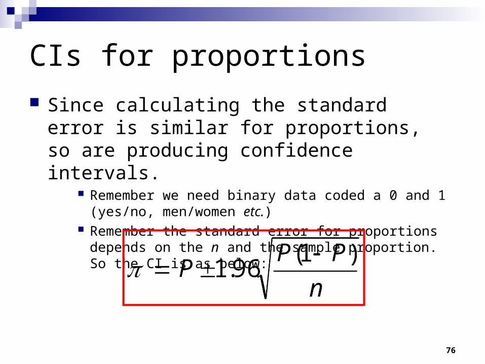
CIs for proportions
Since calculating the standard error is similar for proportions, so are producing confidence intervals.
Remember we need binary data coded a 0 and 1 (yes/no, men/women etc.)
Remember the standard error for proportions depends on the n and the sample proportion. So the CI is as below:

77
Proportions example
Let’s take a political opinion poll in the US, we’re interested in the population proportion voting Democrat (call this π). Sample is 1000 people. Sample proportion is
0.45 (or 45%).

78
Opinion polls
A lot of opinion polls use a sample size of about 1000 people, and aim to estimate proportions that are between 30% and 50%.
This is why you often see ‘margins of error’ that are 3% either side of an estimate quoted in newspapers; these are 95% confidence intervals.
Note that all these confidence intervals ignore non-sampling error.
What we call sampling bias, this could be due to non-response, badly worded questions and so forth.
79
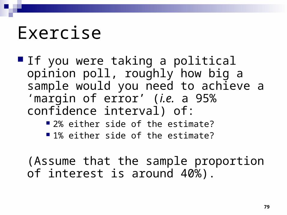
Exercise
If you were taking a political opinion poll, roughly how big a sample would you need to achieve a ‘margin of error’ (i.e. a 95% confidence interval) of:
2% either side of the estimate? 1% either side of the estimate?
(Assume that the sample proportion of interest is around 40%).
80
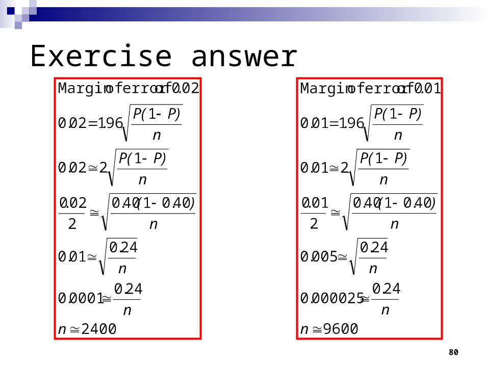
Exercise answer