introduction to data mining bayesian...
TRANSCRIPT
Introduction to Data Mining
Bayesian Classification
CPSC/AMTH 445a/545a
Yale UniversityFall 2016
CPSC 445 (Guy Wolf) Bayesian Classification Yale - Fall 2016 1 / 21
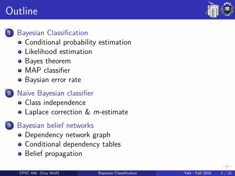
Outline
1 Bayesian ClassificationConditional probability estimationLikelihood estimationBayes theoremMAP classifierBaysian error rate
2 Naıve Bayesian classifierClass independenceLaplace correction & m-estimate
3 Bayesian belief networksDependency network graphConditional dependency tablesBelief propagation
CPSC 445 (Guy Wolf) Bayesian Classification Yale - Fall 2016 2 / 21
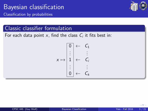
Bayesian classificationClassification by probabilities
Classic classifier formulationFor each data point x , find the class Ci it fits best in:
x 7→
0...1...0
← C1...
← Ci...
← Ck
If we treat the class C and data point x as (hopefully dependent)random variables, we can consider the probabilities Pr[x ∈ Ci ] as theconditional probabilities P(C |x).
CPSC 445 (Guy Wolf) Bayesian Classification Yale - Fall 2016 3 / 21
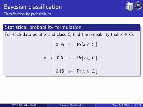
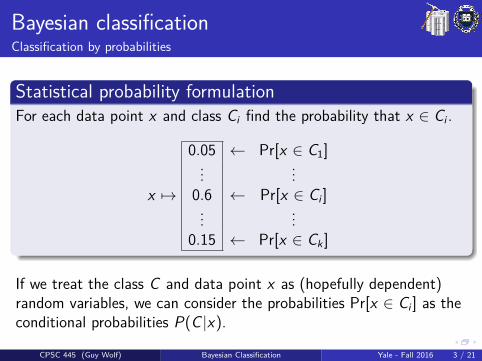
Bayesian classificationClassification by probabilities
Statistical probability formulationFor each data point x and class Ci find the probability that x ∈ Ci .
x 7→
0.05...
0.6...
0.15
← Pr[x ∈ C1]...
← Pr[x ∈ Ci ]...
← Pr[x ∈ Ck ]
If we treat the class C and data point x as (hopefully dependent)random variables, we can consider the probabilities Pr[x ∈ Ci ] as theconditional probabilities P(C |x).
CPSC 445 (Guy Wolf) Bayesian Classification Yale - Fall 2016 3 / 21
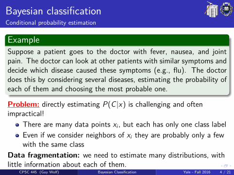
Bayesian classificationConditional probability estimation
ExampleSuppose a patient goes to the doctor with fever, nausea, and jointpain. The doctor can look at other patients with similar symptoms anddecide which disease caused these symptoms (e.g., flu). The doctordoes this by considering several diseases, estimating the probability ofeach of them and choosing the most probable one.
Problem: directly estimating P(C |x) is challenging and oftenimpractical!
There are many data points xi , but each has only one class labelEven if we consider neighbors of xi they are probably only a fewwith the same class
Data fragmentation: we need to estimate many distributions, withlittle information about each of them.
CPSC 445 (Guy Wolf) Bayesian Classification Yale - Fall 2016 4 / 21
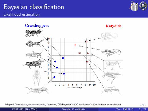
Bayesian classificationLikelihood estimation
Adapted from http://www.cs.ucr.edu/˜eamonn/CE/Bayesian%20Classification%20withInsect examples.pdf
CPSC 445 (Guy Wolf) Bayesian Classification Yale - Fall 2016 5 / 21
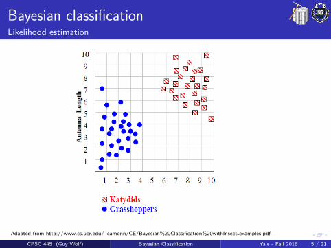
Bayesian classificationLikelihood estimation
Adapted from http://www.cs.ucr.edu/˜eamonn/CE/Bayesian%20Classification%20withInsect examples.pdf
CPSC 445 (Guy Wolf) Bayesian Classification Yale - Fall 2016 5 / 21
Bayesian classificationLikelihood estimation
Adapted from http://www.cs.ucr.edu/˜eamonn/CE/Bayesian%20Classification%20withInsect examples.pdf
CPSC 445 (Guy Wolf) Bayesian Classification Yale - Fall 2016 5 / 21

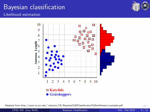
Bayesian classificationLikelihood estimation
Histogram of antenna lengths in each class:
Antenna LengthKatydids Grasshoppers
Adapted from http://www.cs.ucr.edu/˜eamonn/CE/Bayesian%20Classification%20withInsect examples.pdf
CPSC 445 (Guy Wolf) Bayesian Classification Yale - Fall 2016 5 / 21
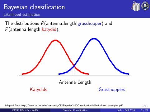
Bayesian classificationLikelihood estimation
The distributions P(antenna length|grasshopper) andP(antenna length|katydid):
Antenna LengthKatydids Grasshoppers
Adapted from http://www.cs.ucr.edu/˜eamonn/CE/Bayesian%20Classification%20withInsect examples.pdf
CPSC 445 (Guy Wolf) Bayesian Classification Yale - Fall 2016 5 / 21
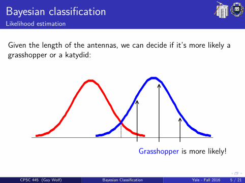
Bayesian classificationLikelihood estimation
Given the length of the antennas, we can decide if it’s more likely agrasshopper or a katydid:
Grasshopper is more likely!
CPSC 445 (Guy Wolf) Bayesian Classification Yale - Fall 2016 5 / 21
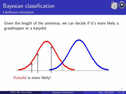
Bayesian classificationLikelihood estimation
Given the length of the antennas, we can decide if it’s more likely agrasshopper or a katydid:
Katydid is more likely!
CPSC 445 (Guy Wolf) Bayesian Classification Yale - Fall 2016 5 / 21
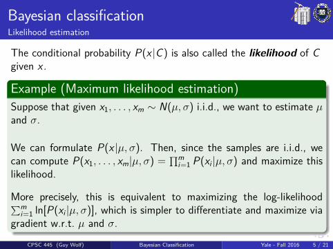
Bayesian classificationLikelihood estimation
The conditional probability P(x |C) is also called the likelihood of Cgiven x .
Example (Maximum likelihood estimation)Suppose that given x1, . . . , xm ∼ N(µ, σ) i.i.d., we want to estimate µand σ.
We can formulate P(x |µ, σ). Then, since the samples are i.i.d., wecan compute P(x1, . . . , xm|µ, σ) = ∏m
i=1 P(xi |µ, σ) and maximize thislikelihood.
More precisely, this is equivalent to maximizing the log-likelihood∑mi=1 ln[P(xi |µ, σ)], which is simpler to differentiate and maximize via
gradient w.r.t. µ and σ.
CPSC 445 (Guy Wolf) Bayesian Classification Yale - Fall 2016 5 / 21
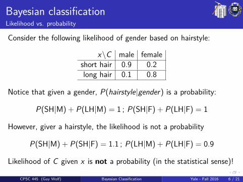
Bayesian classificationLikelihood vs. probability
Consider the following likelihood of gender based on hairstyle:
x\C male femaleshort hair 0.9 0.2long hair 0.1 0.8
Notice that given a gender, P(hairstyle|gender) is a probability:
P(SH|M) + P(LH|M) = 1 ; P(SH|F) + P(LH|F) = 1
However, giver a hairstyle, the likelihood is not a probability
P(SH|M) + P(SH|F) = 1.1 ; P(LH|M) + P(LH|F) = 0.9
Likelihood of C given x is not a probability (in the statistical sense)!
CPSC 445 (Guy Wolf) Bayesian Classification Yale - Fall 2016 6 / 21
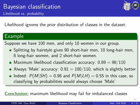
Bayesian classificationLikelihood vs. probability
Likelihood ignores the prior distribution of classes in the dataset:
ExampleSuppose we have 100 men, and only 10 women in our group.
Splitting by hairstyle gives 90 short-hair men, 10 long-hair men,8 long-hair women, and 2 short-hair women.Maximum likelihood classification accuracy: 0.89 = 98/110Always ‘Male’ accuracy: 0.91 = 100/110, which is slightly betterIndeed: P(M|SH) = 0.98 and P(M|LH) = 0.55 in this case, soclassifying by probabilities would always choose ‘Male’
Conclusion: maximum likelihood may fail for imbalanced classes
CPSC 445 (Guy Wolf) Bayesian Classification Yale - Fall 2016 6 / 21
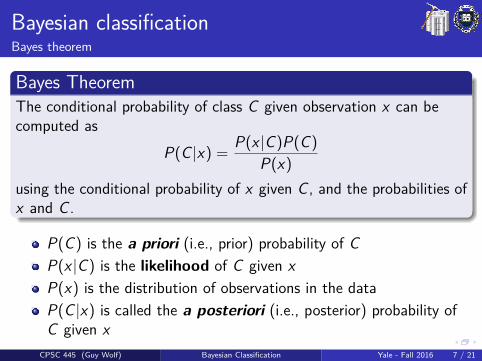
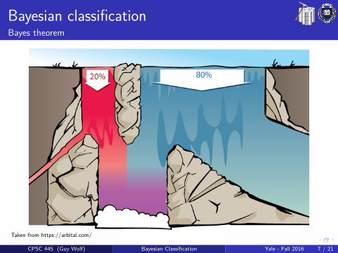
Bayesian classificationBayes theorem
Bayes TheoremThe conditional probability of class C given observation x can becomputed as
P(C |x) = P(x |C)P(C)P(x)
using the conditional probability of x given C , and the probabilities ofx and C .
P(C) is the a priori (i.e., prior) probability of CP(x |C) is the likelihood of C given xP(x) is the distribution of observations in the dataP(C |x) is called the a posteriori (i.e., posterior) probability ofC given x
CPSC 445 (Guy Wolf) Bayesian Classification Yale - Fall 2016 7 / 21

Bayesian classificationBayes theorem
Taken from https://arbital.com/
CPSC 445 (Guy Wolf) Bayesian Classification Yale - Fall 2016 7 / 21
Bayesian classificationBayes theorem
Taken from https://arbital.com/
CPSC 445 (Guy Wolf) Bayesian Classification Yale - Fall 2016 7 / 21

Bayesian classificationBayes theorem
Taken from https://arbital.com/
CPSC 445 (Guy Wolf) Bayesian Classification Yale - Fall 2016 7 / 21

Bayesian classificationBayes theorem
Taken from https://arbital.com/CPSC 445 (Guy Wolf) Bayesian Classification Yale - Fall 2016 7 / 21

Bayesian classificationMaximum a posteriori (MAP) classifier
Bayesian classification is uses the class prior and likelihood toestimate the class posterior, and classify by maximum a posterioriprobability:
Training1 Estimate the prior P(C) from class sizes in data2 For each class C , estimate P(x |C):
If x is categorical/discrete, just count valuesIf x is continuous, either discretize or estimate predetermineddistribution (e.g., Gaussian or Poisson)
TestingFor each x choose the class C that maximizes P(x |C)P(C).
CPSC 445 (Guy Wolf) Bayesian Classification Yale - Fall 2016 8 / 21
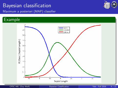
Bayesian classificationMaximum a posteriori (MAP) classifier
Example
CPSC 445 (Guy Wolf) Bayesian Classification Yale - Fall 2016 8 / 21
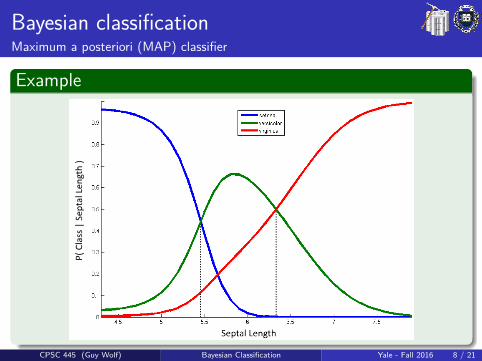
Bayesian classificationMaximum a posteriori (MAP) classifier
Example
CPSC 445 (Guy Wolf) Bayesian Classification Yale - Fall 2016 8 / 21
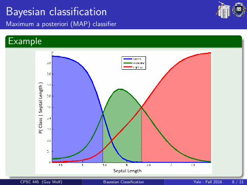
Bayesian classificationMaximum a posteriori (MAP) classifier
Example
CPSC 445 (Guy Wolf) Bayesian Classification Yale - Fall 2016 8 / 21
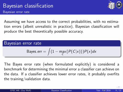
Bayesian classificationBayesian error rate
Assuming we have access to the correct probabilities, with no estima-tion errors (albeit unrealistic in practice), Bayesian classification willproduce the best theoretically possible accuracy.
Bayesian error rateBayes err =
∫(1−max
C{P(C |x)})P(x)dx
The Bayes error rate (when formulated explicitly) is considered abenchmark for determining the minimal error a classifier can achieve onthe data. If a classifier achieves lower error rates, it probably overfitsthe training/validation data.
CPSC 445 (Guy Wolf) Bayesian Classification Yale - Fall 2016 9 / 21
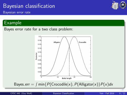
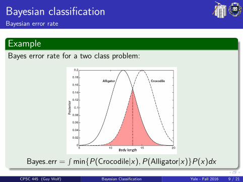
Bayesian classificationBayesian error rate
ExampleBayes error rate for a two class problem:
Bayes err =∫
min{P(Crocodile|x),P(Alligator|x)}P(x)dx
CPSC 445 (Guy Wolf) Bayesian Classification Yale - Fall 2016 9 / 21
Bayesian classificationBayesian error rate
ExampleBayes error rate for a two class problem:
Bayes err =∫
min{P(Crocodile|x),P(Alligator|x)}P(x)dx
CPSC 445 (Guy Wolf) Bayesian Classification Yale - Fall 2016 9 / 21
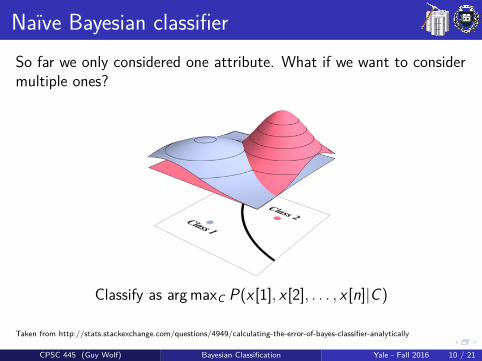
Naıve Bayesian classifierSo far we only considered one attribute. What if we want to considermultiple ones?
Classify as arg maxC P(x [1], x [2], . . . , x [n]|C)
Taken from http://stats.stackexchange.com/questions/4949/calculating-the-error-of-bayes-classifier-analytically
CPSC 445 (Guy Wolf) Bayesian Classification Yale - Fall 2016 10 / 21
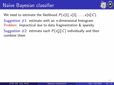
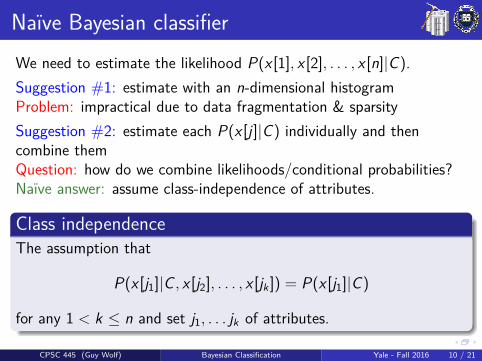
Naıve Bayesian classifierWe need to estimate the likelihood P(x [1], x [2], . . . , x [n]|C).
Suggestion #1: estimate with an n-dimensional histogramProblem: impractical due to data fragmentation & sparsitySuggestion #2: estimate each P(x [j ]|C) individually and thencombine themQuestion: how do we combine likelihoods/conditional probabilities?Naıve answer: assume class-independence of attributes.
Class independenceThe assumption that
P(x [j1]|C , x [j2], . . . , x [jk ]) = P(x [j1]|C)
for any 1 < k ≤ n and set j1, . . . jk of attributes.
CPSC 445 (Guy Wolf) Bayesian Classification Yale - Fall 2016 10 / 21
Naıve Bayesian classifierWe need to estimate the likelihood P(x [1], x [2], . . . , x [n]|C).Suggestion #1: estimate with an n-dimensional histogram
Problem: impractical due to data fragmentation & sparsitySuggestion #2: estimate each P(x [j ]|C) individually and thencombine themQuestion: how do we combine likelihoods/conditional probabilities?Naıve answer: assume class-independence of attributes.
Class independenceThe assumption that
P(x [j1]|C , x [j2], . . . , x [jk ]) = P(x [j1]|C)
for any 1 < k ≤ n and set j1, . . . jk of attributes.
CPSC 445 (Guy Wolf) Bayesian Classification Yale - Fall 2016 10 / 21
Naıve Bayesian classifierWe need to estimate the likelihood P(x [1], x [2], . . . , x [n]|C).Suggestion #1: estimate with an n-dimensional histogramProblem: impractical due to data fragmentation & sparsity
Suggestion #2: estimate each P(x [j ]|C) individually and thencombine themQuestion: how do we combine likelihoods/conditional probabilities?Naıve answer: assume class-independence of attributes.
Class independenceThe assumption that
P(x [j1]|C , x [j2], . . . , x [jk ]) = P(x [j1]|C)
for any 1 < k ≤ n and set j1, . . . jk of attributes.
CPSC 445 (Guy Wolf) Bayesian Classification Yale - Fall 2016 10 / 21
Naıve Bayesian classifierWe need to estimate the likelihood P(x [1], x [2], . . . , x [n]|C).Suggestion #1: estimate with an n-dimensional histogramProblem: impractical due to data fragmentation & sparsitySuggestion #2: estimate each P(x [j ]|C) individually and thencombine them
Question: how do we combine likelihoods/conditional probabilities?Naıve answer: assume class-independence of attributes.
Class independenceThe assumption that
P(x [j1]|C , x [j2], . . . , x [jk ]) = P(x [j1]|C)
for any 1 < k ≤ n and set j1, . . . jk of attributes.
CPSC 445 (Guy Wolf) Bayesian Classification Yale - Fall 2016 10 / 21
Naıve Bayesian classifierWe need to estimate the likelihood P(x [1], x [2], . . . , x [n]|C).Suggestion #1: estimate with an n-dimensional histogramProblem: impractical due to data fragmentation & sparsitySuggestion #2: estimate each P(x [j ]|C) individually and thencombine themQuestion: how do we combine likelihoods/conditional probabilities?
Naıve answer: assume class-independence of attributes.
Class independenceThe assumption that
P(x [j1]|C , x [j2], . . . , x [jk ]) = P(x [j1]|C)
for any 1 < k ≤ n and set j1, . . . jk of attributes.
CPSC 445 (Guy Wolf) Bayesian Classification Yale - Fall 2016 10 / 21
Naıve Bayesian classifierWe need to estimate the likelihood P(x [1], x [2], . . . , x [n]|C).Suggestion #1: estimate with an n-dimensional histogramProblem: impractical due to data fragmentation & sparsitySuggestion #2: estimate each P(x [j ]|C) individually and thencombine themQuestion: how do we combine likelihoods/conditional probabilities?Naıve answer: assume class-independence of attributes.
Class independenceThe assumption that
P(x [j1]|C , x [j2], . . . , x [jk ]) = P(x [j1]|C)
for any 1 < k ≤ n and set j1, . . . jk of attributes.
CPSC 445 (Guy Wolf) Bayesian Classification Yale - Fall 2016 10 / 21
Naıve Bayesian classifierClass independence
Under the class independence assumption we can compute for any i , j :P(x [i ], x [k]|C) = P(x [i ]|C , x [k])P(x [k]|C) = P(x [i ]|C)P(x [k]|C)
Similarly, for n attributes we have:
P(~x |C) = P(x [1], x [2], · · · , x [n]|C) =n∏
j=1P(x [j ]|C)
Therefore, we can formulate a multivariate classifier as follows:Naıve Bayes classificationTraining: For each class C and attribute j = 1, . . . , n,
estimate P(C) and P(x [j ]|C) from training data;Testing: Classify each data point x (e.g., in test/validation data)
as arg maxC P(C) ∏nj=1 P(x [j ]|C) .
CPSC 445 (Guy Wolf) Bayesian Classification Yale - Fall 2016 11 / 21
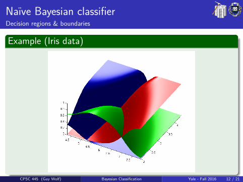
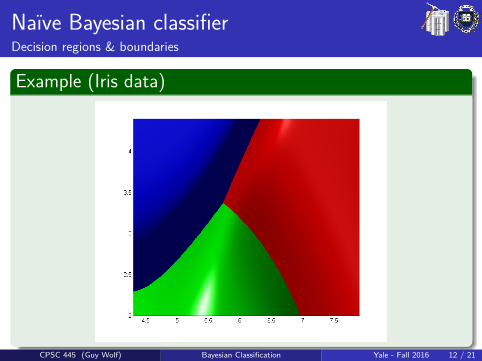
Naıve Bayesian classifierDecision regions & boundaries
Example (Iris data)
CPSC 445 (Guy Wolf) Bayesian Classification Yale - Fall 2016 12 / 21
Naıve Bayesian classifierDecision regions & boundaries
Example (Iris data)
CPSC 445 (Guy Wolf) Bayesian Classification Yale - Fall 2016 12 / 21
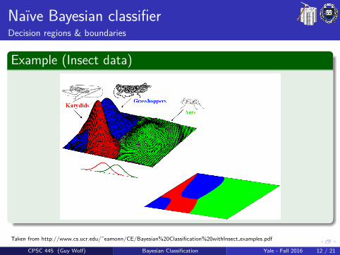
Naıve Bayesian classifierDecision regions & boundaries
Example (Insect data)
Taken from http://www.cs.ucr.edu/˜eamonn/CE/Bayesian%20Classification%20withInsect examples.pdf
CPSC 445 (Guy Wolf) Bayesian Classification Yale - Fall 2016 12 / 21
Naıve Bayesian classifierLaplace correction & m-estimate
If Pr[x [j ] = a|C = Ci ] ≈ 0 due to data sparsity, the posterior of any{x : x [j ] = a} will be zero, even if other attributes strongly predict Ci .
This can be alleviated by two correction methods:
Laplace correctionAssume all counters used by estimators are large enough that we cansafely add 1 to them to get Pr[x [j ] = a|C = Ci ] ≈ #{x :x [j]=a∧x∈Ci }+1
#{x :x∈Ci }+1
m-estimateGeneralize the Laplace correction toPr[x [j ] = a|C = Ci ] ≈ #{x :x [j]=a∧x∈Ci }+mp
#{x :x∈Ci }+m , where 0 < p ≤ 1 is anassumed likelihood prior and m is our confidence in this assumption.
CPSC 445 (Guy Wolf) Bayesian Classification Yale - Fall 2016 13 / 21
Bayesian belief networksNaıve Bayes assumes class independence to simplify probabilityestimations, but this is not always applicable.
ExampleSuppose we see the grass is wet, and we want to assess whether:
it was raining, orthe sprinklers were on.
If the sprinklers are always on from 4:00 AM to 5:00 AM, we canassume independence between these causes and estimate using thetime and grass wetness.However, if “smart” sprinklers only turn on when tonight wasn’t rainyenough, we should considers some conditional dependencyP(sprinklers|rain) 6= 0.
How do we model conditional dependencies in an efficient way?CPSC 445 (Guy Wolf) Bayesian Classification Yale - Fall 2016 14 / 21
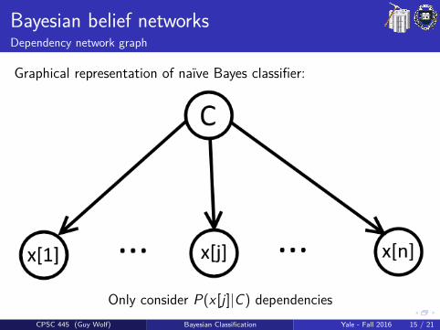
Bayesian belief networksDependency network graph
Graphical representation of naıve Bayes classifier:
Only consider P(x [j ]|C) dependenciesCPSC 445 (Guy Wolf) Bayesian Classification Yale - Fall 2016 15 / 21
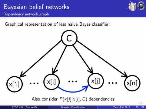
Bayesian belief networksDependency network graph
Graphical representation of less naıve Bayes classifier:
Also consider P(x [j ]|x [i ],C) dependenciesCPSC 445 (Guy Wolf) Bayesian Classification Yale - Fall 2016 15 / 21
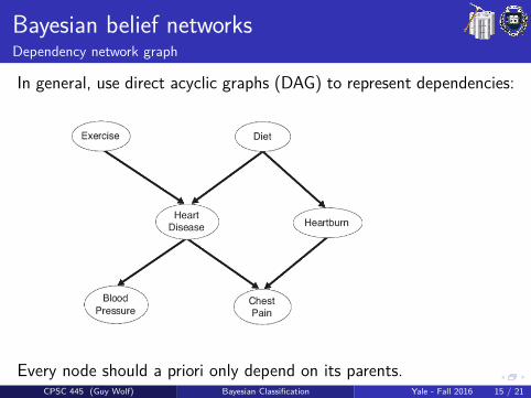
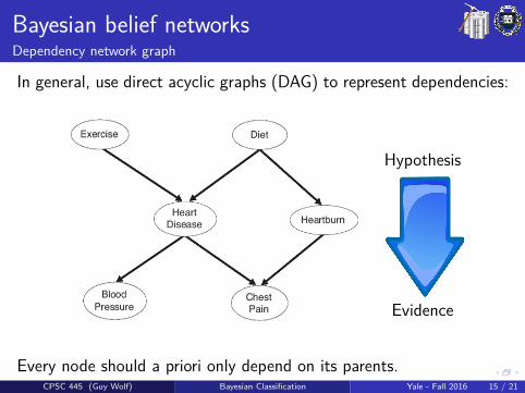
Bayesian belief networksDependency network graph
In general, use direct acyclic graphs (DAG) to represent dependencies:
Cause
Effect
Hypothesis
Evidence
Every node should a priori only depend on its parents.CPSC 445 (Guy Wolf) Bayesian Classification Yale - Fall 2016 15 / 21

Bayesian belief networksDependency network graph
In general, use direct acyclic graphs (DAG) to represent dependencies:
Cause
Effect
Hypothesis
Evidence
Every node should a priori only depend on its parents.CPSC 445 (Guy Wolf) Bayesian Classification Yale - Fall 2016 15 / 21
Bayesian belief networksDependency network graph
In general, use direct acyclic graphs (DAG) to represent dependencies:
Cause
Effect
Hypothesis
Evidence
Every node should a priori only depend on its parents.CPSC 445 (Guy Wolf) Bayesian Classification Yale - Fall 2016 15 / 21
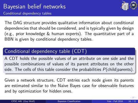
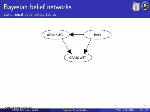
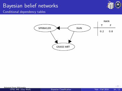
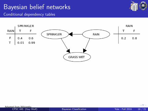
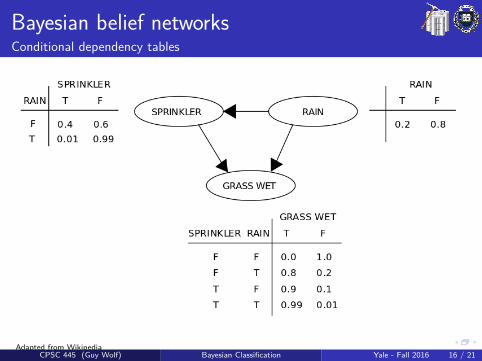
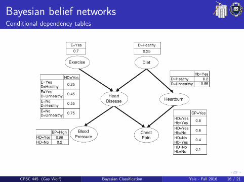
Bayesian belief networksConditional dependency tables
The DAG structure provides qualitative information about conditionaldependencies that should be considered, and is typically given by design(e.g., prior knowledge & human experts). The quantitative part of aBBN is given by conditional dependency tables.
Conditional dependency table (CDT)A CDT holds the possible values of an attribute on one side and thepossible combinations of values of its parent attributes on the otherside. The cells of this table consider the probabilities P(child|parents).
Given a network structure, CDT entries each node given its parentsare estimated similar to the Naıve Bayes case for observable featuresand by optimization for hidden ones.
CPSC 445 (Guy Wolf) Bayesian Classification Yale - Fall 2016 16 / 21
Bayesian belief networksConditional dependency tables
Adapted from WikipediaCPSC 445 (Guy Wolf) Bayesian Classification Yale - Fall 2016 16 / 21
Bayesian belief networksConditional dependency tables
Adapted from WikipediaCPSC 445 (Guy Wolf) Bayesian Classification Yale - Fall 2016 16 / 21
Bayesian belief networksConditional dependency tables
Adapted from WikipediaCPSC 445 (Guy Wolf) Bayesian Classification Yale - Fall 2016 16 / 21
Bayesian belief networksConditional dependency tables
Adapted from WikipediaCPSC 445 (Guy Wolf) Bayesian Classification Yale - Fall 2016 16 / 21
Bayesian belief networksConditional dependency tables
CPSC 445 (Guy Wolf) Bayesian Classification Yale - Fall 2016 16 / 21
Bayesian belief networksConditional dependency tables
CPSC 445 (Guy Wolf) Bayesian Classification Yale - Fall 2016 16 / 21
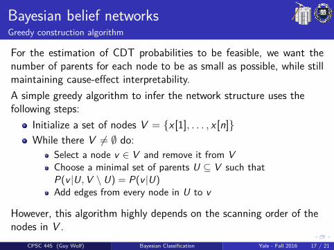
Bayesian belief networksGreedy construction algorithm
For the estimation of CDT probabilities to be feasible, we want thenumber of parents for each node to be as small as possible, while stillmaintaining cause-effect interpretability.A simple greedy algorithm to infer the network structure uses thefollowing steps:
Initialize a set of nodes V = {x [1], . . . , x [n]}While there V 6= ∅ do:
Select a node v ∈ V and remove it from VChoose a minimal set of parents U ⊆ V such thatP(v |U, V \ U) = P(v |U)Add edges from every node in U to v
However, this algorithm highly depends on the scanning order of thenodes in V .
CPSC 445 (Guy Wolf) Bayesian Classification Yale - Fall 2016 17 / 21
Bayesian belief networksGreedy construction algorithm
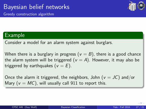
ExampleConsider a model for an alarm system against burglars.
When there is a burglary in progress (v = B), there is a good chancethe alarm system will be triggered (v = A). However, it may also betriggered by earthquakes (v = E ).
Once the alarm it triggered, the neighbors, John (v = JC) and/orMary (v = MC), will usually call 911 to report this.
CPSC 445 (Guy Wolf) Bayesian Classification Yale - Fall 2016 17 / 21
Bayesian belief networksGreedy construction algorithm
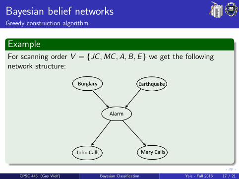
ExampleFor scanning order V = {JC ,MC ,A,B,E} we get the followingnetwork structure:
CPSC 445 (Guy Wolf) Bayesian Classification Yale - Fall 2016 17 / 21
Bayesian belief networksGreedy construction algorithm
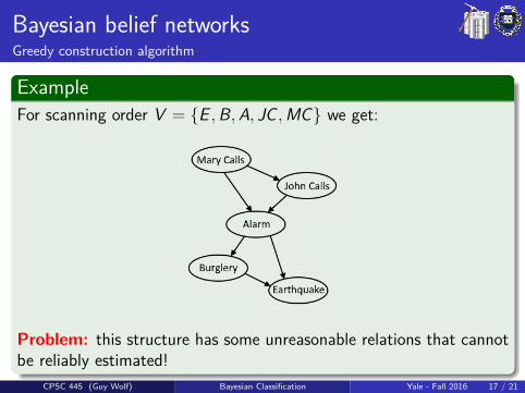
ExampleFor scanning order V = {E ,B,A, JC ,MC} we get:
Problem: this structure has some unreasonable relations that cannotbe reliably estimated!
CPSC 445 (Guy Wolf) Bayesian Classification Yale - Fall 2016 17 / 21
Bayesian belief networksGreedy construction algorithm
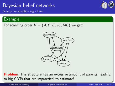
ExampleFor scanning order V = {A,B,E , JC ,MC} we get:
Problem: this structure has an excessive amount of parents, leadingto big CDTs that are impractical to estimate!
CPSC 445 (Guy Wolf) Bayesian Classification Yale - Fall 2016 17 / 21
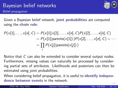
Bayesian belief networksBelief propagation
Given a Bayesian belief network, joint probabilities are computedusing the chain rule:
P(x [1], . . . , x [n],C) = P(x [1]|x [2], . . . , x [n],C)P(x [2], . . . , x [n],C)= P(x [1]|parents(x [1]) )P(x [2], . . . , x [n],C) = · · ·=
∏j
P(x [j ]|parents(x [j ]) )
Notice that C can also be extended to consider several output nodes.Furthermore, missing values can naturally be processed by consider-ing partial sets of attributes. Likelihoods and posteriors can then beestimated using joint probabilities.When considering belief propagation, it is useful to identify indepen-dence between events in the network.
CPSC 445 (Guy Wolf) Bayesian Classification Yale - Fall 2016 18 / 21
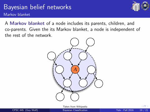
Bayesian belief networksMarkov blanket
A Markov blanket of a node includes its parents, children, andco-parents. Given the its Markov blanket, a node is independent ofthe rest of the network.
Taken from WikipediaCPSC 445 (Guy Wolf) Bayesian Classification Yale - Fall 2016 19 / 21
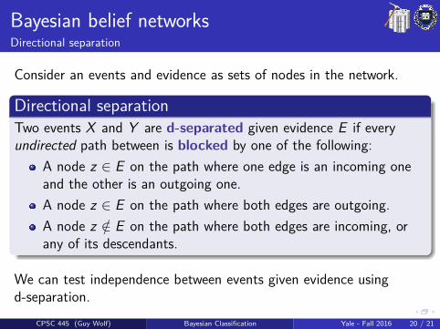
Bayesian belief networksDirectional separation
Consider an events and evidence as sets of nodes in the network.
Directional separationTwo events X and Y are d-separated given evidence E if everyundirected path between is blocked by one of the following:
A node z ∈ E on the path where one edge is an incoming oneand the other is an outgoing one.A node z ∈ E on the path where both edges are outgoing.A node z /∈ E on the path where both edges are incoming, orany of its descendants.
We can test independence between events given evidence usingd-separation.
CPSC 445 (Guy Wolf) Bayesian Classification Yale - Fall 2016 20 / 21
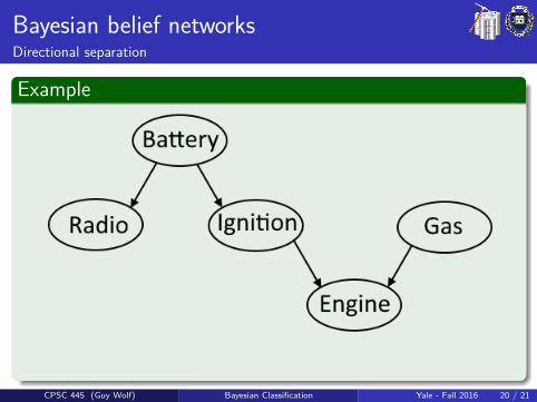
Bayesian belief networksDirectional separation
Example
CPSC 445 (Guy Wolf) Bayesian Classification Yale - Fall 2016 20 / 21
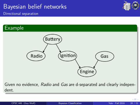
Bayesian belief networksDirectional separation
Example
Given no evidence, Radio and Gas are d-separated and clearly indepen-dent.
CPSC 445 (Guy Wolf) Bayesian Classification Yale - Fall 2016 20 / 21
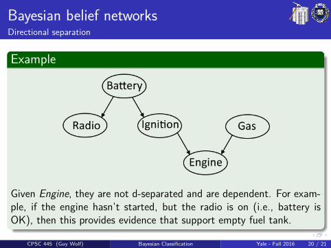
Bayesian belief networksDirectional separation
Example
Given Engine, they are not d-separated and are dependent. For exam-ple, if the engine hasn’t started, but the radio is on (i.e., battery isOK), then this provides evidence that support empty fuel tank.
CPSC 445 (Guy Wolf) Bayesian Classification Yale - Fall 2016 20 / 21
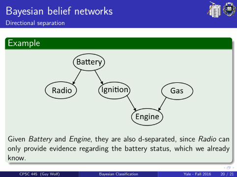
Bayesian belief networksDirectional separation
Example
Given Battery and Engine, they are also d-separated, since Radio canonly provide evidence regarding the battery status, which we alreadyknow.
CPSC 445 (Guy Wolf) Bayesian Classification Yale - Fall 2016 20 / 21
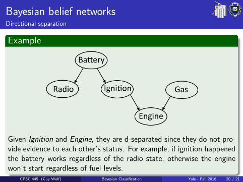
Bayesian belief networksDirectional separation
Example
Given Ignition and Engine, they are d-separated since they do not pro-vide evidence to each other’s status. For example, if ignition happenedthe battery works regardless of the radio state, otherwise the enginewon’t start regardless of fuel levels.
CPSC 445 (Guy Wolf) Bayesian Classification Yale - Fall 2016 20 / 21
SummaryBayesian classification aims to choose the most probable/likely classbased on observed attributes
Maximum likelihood estimation can be used when classes arebalancedBayes theorem enables maximum a posteriori estimation
For multivariate data, estimated likelihoods should be combined toget MAP estimation
Naive Bayes classifier assumes class conditional independenceBayesian belief networks use a DAG and CDTs to estimate andcombine conditional probabilities
With no estimation errors, this approach achieves the best possibleclassification results. However, in realistic scenarios results dependheavily on accurate estimation of the probabilities involved in it.
CPSC 445 (Guy Wolf) Bayesian Classification Yale - Fall 2016 21 / 21