introduction to data mining using weka
TRANSCRIPT

Introduction to Data Mining Using Weka
Asst. Prof. Peerasak Intarapaiboon, Ph.D.
List of Topics
• Part-I: Introduction to data mining• Basic concepts
• Applications in the business’s world
• More details: tasks, learning algorithms, processes, etc.
• Some focused models
• Part-II: Quick tour in Weka• What is Weka?
• How to install Weka
• Fundamental tools in Weka
• Let’s start to use Weka
Workshop@TU 2

Workshop@TU 3

Applications of DM: Where are you?
Workshop@TU 4

Applications of DM: Where are you?
Workshop@TU 5
RecommendationSystems

Applications of DM: Where are you?
Workshop@TU 6

• Market Basket Analysis• “if you buy a certain group of items, you are more (or less) likely to buy
another group of items, e.g. IF {beer, no bar meal} THEN {crisps}.”
• Customer Relationship Management• improve customers’ loyalty and implementing customer focused strategies
• Financial Banking• E.g. Credit Risk, Trading, Financial Market Risk
Workshop@TU 7
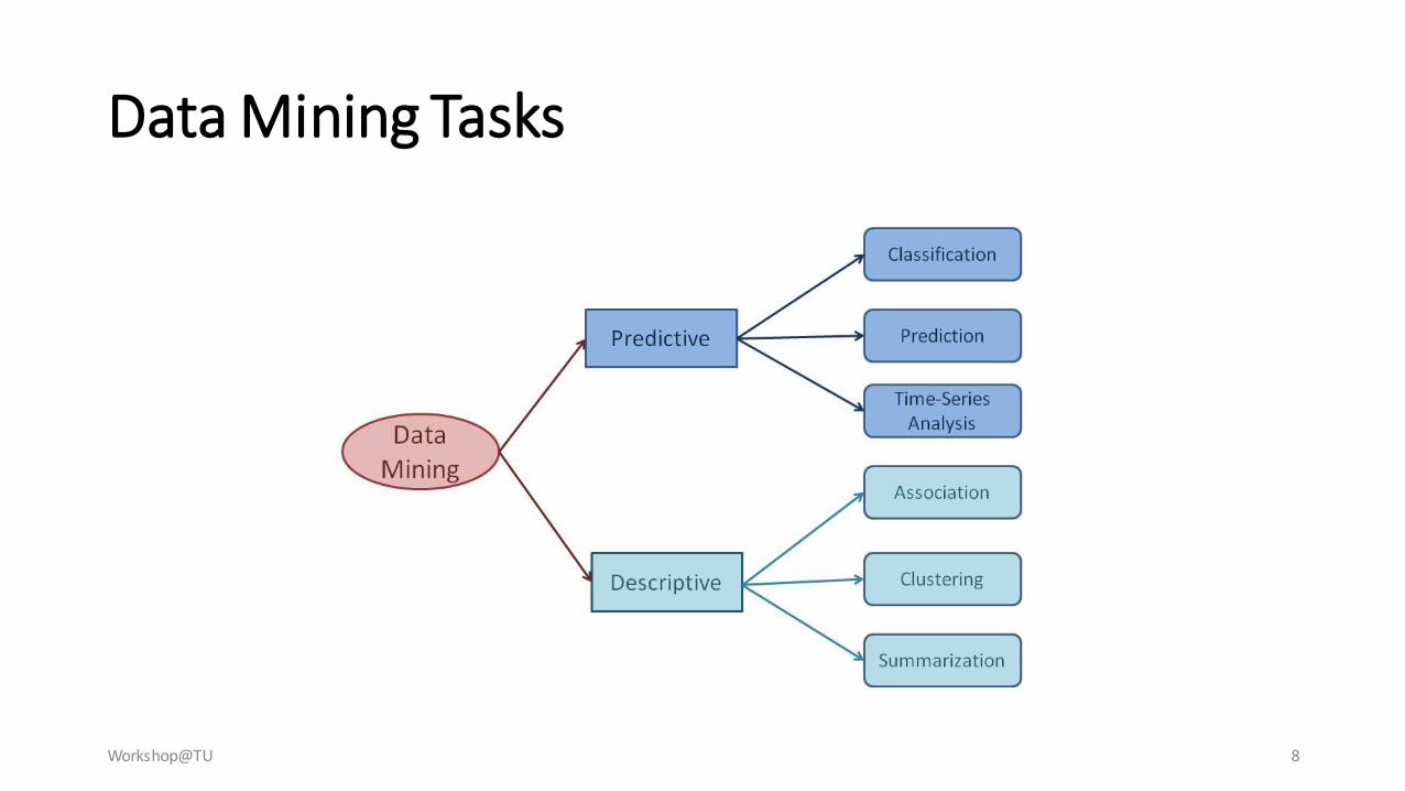
Data Mining Tasks
Workshop@TU 8
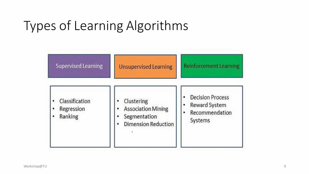
Types of Learning Algorithms
Workshop@TU 9
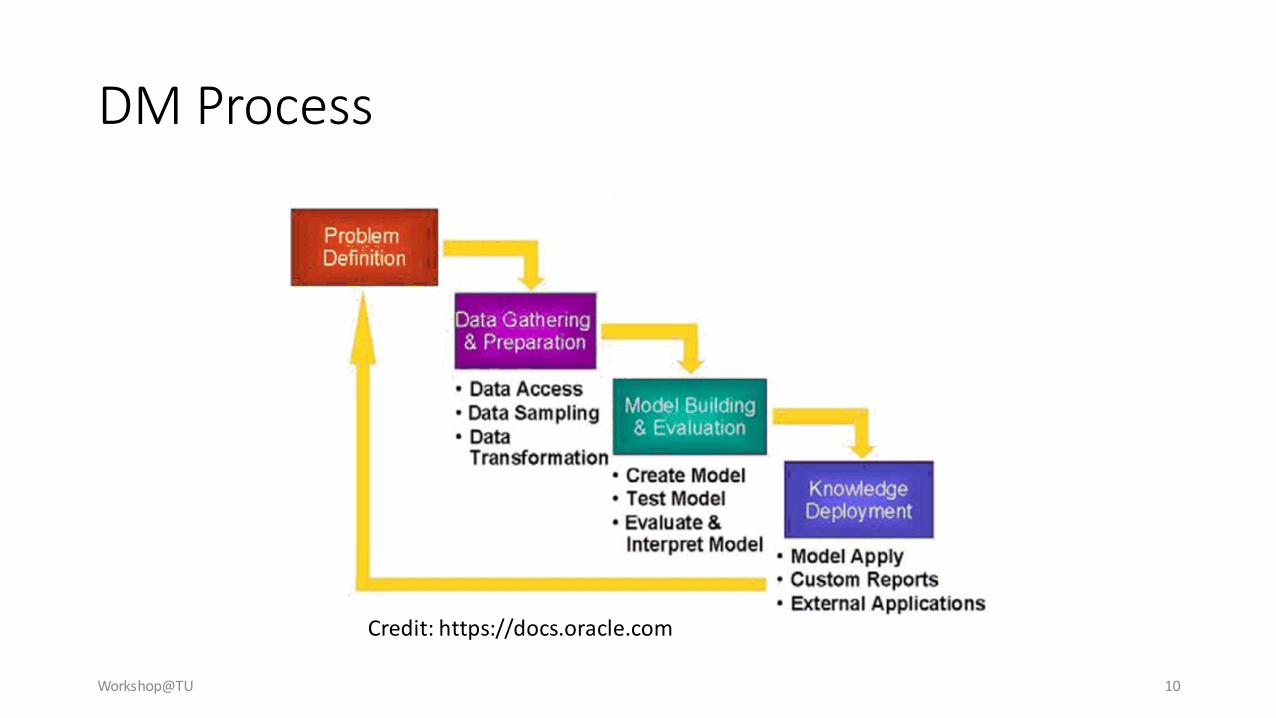
DM Process
Workshop@TU 10
Credit: https://docs.oracle.com
Workshop@TU 11
• Classification by decision tree induction
• Bayesian classification
• Rule-based classification
• Classification by back propagation
• Support Vector Machines (SVM)
• Associative classification
• Lazy learners (or learning from your neighbors)
Classification

Workshop@TU 12
age income student credit_rating buys_computer
<=30 high no fair no
<=30 high no excellent no
31…40 high no fair yes
>40 medium no fair yes
>40 low yes fair yes
>40 low yes excellent no
31…40 low yes excellent yes
<=30 medium no fair no
<=30 low yes fair yes
>40 medium yes fair yes
<=30 medium yes excellent yes
31…40 medium no excellent yes
31…40 high yes fair yes
>40 medium no excellent no
1. Classification: Decision Tree
Workshop@TU 13
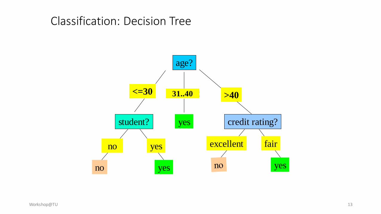
Classification: Decision Tree
age?
overcast
student? credit rating?
<=30 >40
no yes yes
yes
31..40
fairexcellentyesno
Workshop@TU 14
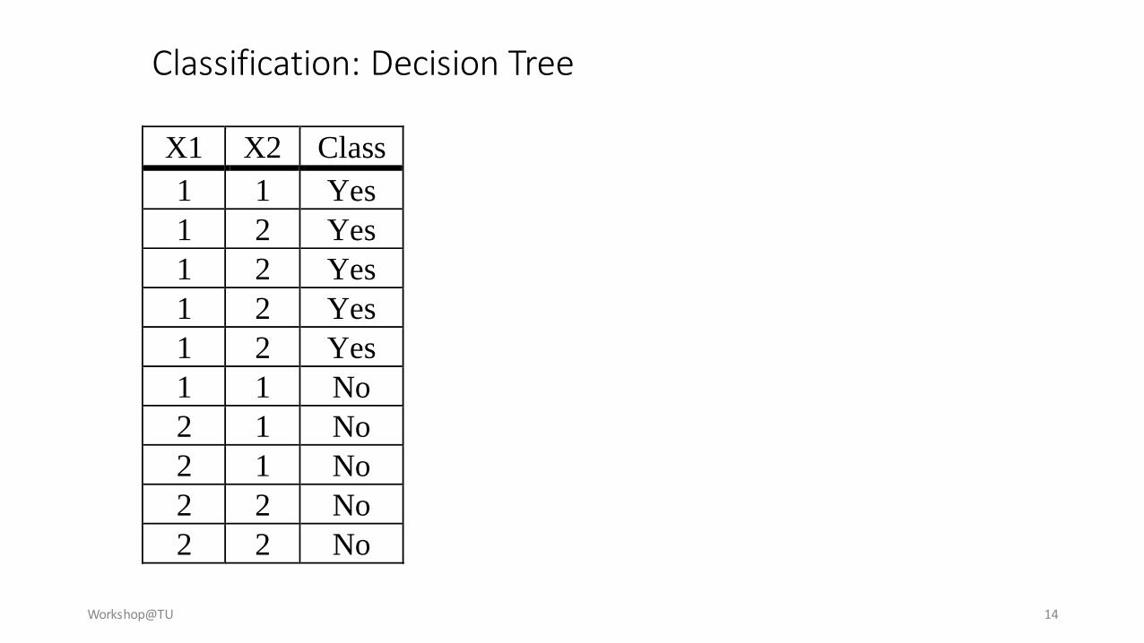
X1 X2 Class
1 1 Yes
1 2 Yes
1 2 Yes
1 2 Yes
1 2 Yes
1 1 No
2 1 No
2 1 No
2 2 No
2 2 No
Classification: Decision Tree

Workshop@TU 15
X1 X2 Class
1 1 Yes
1 2 Yes
1 2 Yes
1 2 Yes
1 2 Yes
1 1 No
2 1 No
2 1 No
2 2 No
2 2 No
X1
X2
Yes
(83%,17%)
No
(25%,75%)
No
(0%,100%)
Yes
(66%,33%)
Classification: Decision Tree
1 2
1 2
Workshop@TU 16
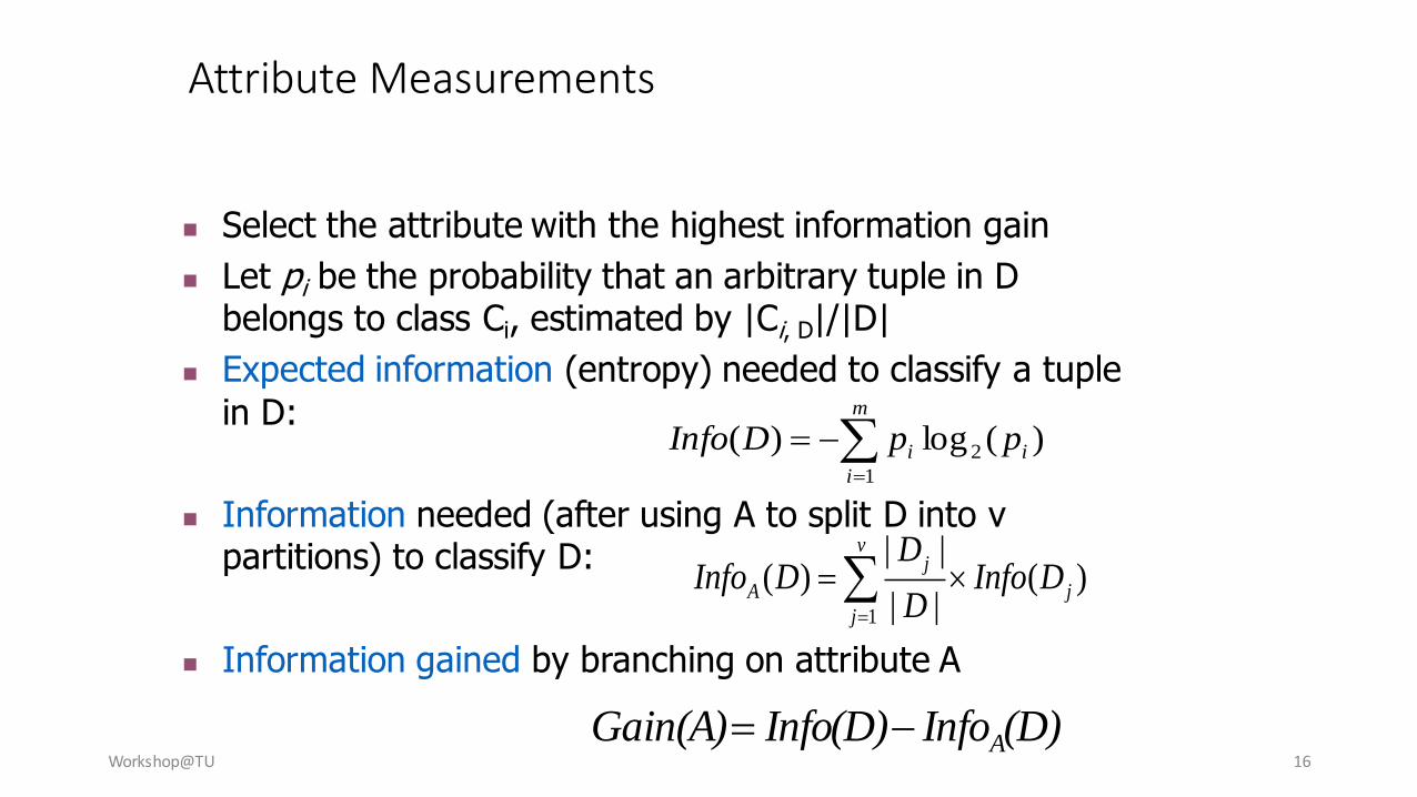
Select the attribute with the highest information gain
Let pi be the probability that an arbitrary tuple in D belongs to class Ci, estimated by |Ci, D|/|D|
Expected information (entropy) needed to classify a tuple
in D:
Information needed (after using A to split D into v partitions) to classify D:
Information gained by branching on attribute A
)(log)( 2
1
i
m
i
i ppDInfo
1
| |( ) ( )
| |
vj
A j
j
DInfo D Info D
D
(D)InfoInfo(D)Gain(A) A
Attribute Measurements
Workshop 1
• Create a decision tree from “ComPurchase.csv” and “TicTacToe.csv”
• Explore the weka environment• Data loading
• Data information
• Model learning
• Model evaluation
Workshop@TU 17
Workshop@TU 18
Discretization
• Three types of attributes:
• Nominal — values from an unordered set, e.g., color, profession
• Ordinal — values from an ordered set, e.g., military or academic rank
• Continuous — real numbers, e.g., integer or real numbers
• Discretization:
• Divide the range of a continuous attribute into intervals
• Some classification algorithms only accept categorical attributes.
• Reduce data size by discretization
• Prepare for further analysis

Workshop@TU 19
Unsupervised Method
Equal Frequency Discretization
Discretization
Equal Width Discretization
Supervised Method
Hours Studied A on Test
4 N
5 Y
8 N
12 Y
15 Y
<=6.5 1 1
>6.5 2 1
A Less than A
Entropy(G1) = 1
Entropy(G2) = 0.971
Overall = (2/5)(1) + (3/5)(0.971) = 0.983

Workshop 2
• How to handle numeric attributes• Discretization
• Use “Iris.csv”
• Data type• Use “Car.csv”
Workshop@TU 20
Workshop@TU 21
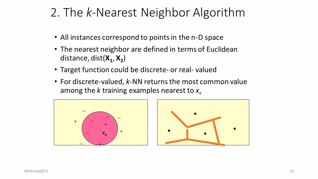
2. The k-Nearest Neighbor Algorithm
• All instances correspond to points in the n-D space
• The nearest neighbor are defined in terms of Euclidean distance, dist(X1, X2)
• Target function could be discrete- or real- valued
• For discrete-valued, k-NN returns the most common value among the k training examples nearest to xq
.
_+
_ xq
+
_ _+
_
_
+
.
.. .

Workshop 3
• Apply kNN to “Iris.csv”
• Compare with the results in Workshop 2
Workshop@TU 22
Workshop@TU 23
3. Bayesian Classification• A statistical classifier: performs probabilistic prediction, i.e.,
predicts class membership probabilities
• Foundation: Based on Bayes’ Theorem.
• Performance: A simple Bayesian classifier, naïve Bayesian classifier, has comparable performance with decision tree and selected neural network classifiers
• Incremental: Each training example can incrementally increase/decrease the probability that a hypothesis is correct —prior knowledge can be combined with observed data
• Standard: Even when Bayesian methods are computationally intractable, they can provide a standard of optimal decision making against which other methods can be measured
Workshop@TU 24
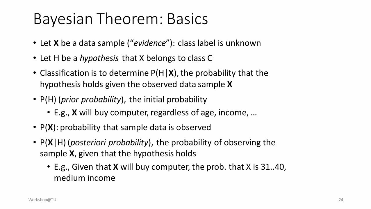
Bayesian Theorem: Basics
• Let X be a data sample (“evidence”): class label is unknown
• Let H be a hypothesis that X belongs to class C
• Classification is to determine P(H|X), the probability that the hypothesis holds given the observed data sample X
• P(H) (prior probability), the initial probability
• E.g., X will buy computer, regardless of age, income, …
• P(X): probability that sample data is observed
• P(X|H) (posteriori probability), the probability of observing the sample X, given that the hypothesis holds
• E.g., Given that X will buy computer, the prob. that X is 31..40, medium income
Workshop@TU 25
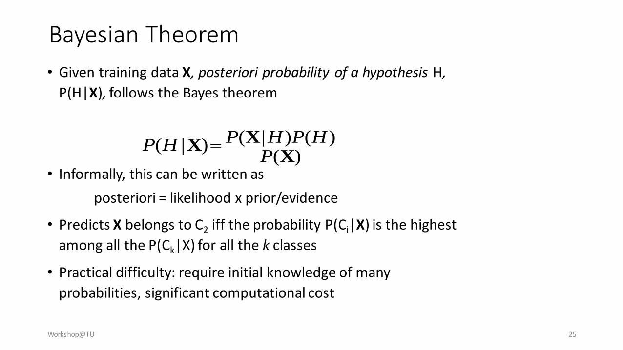
Bayesian Theorem
• Given training data X, posteriori probability of a hypothesis H,
P(H|X), follows the Bayes theorem
• Informally, this can be written as
posteriori = likelihood x prior/evidence
• Predicts X belongs to C2 iff the probability P(Ci|X) is the highest
among all the P(Ck|X) for all the k classes
• Practical difficulty: require initial knowledge of many
probabilities, significant computational cost
)()()|()|(
XXX
PHPHPHP

Workshop@TU 26
Towards Naïve Bayesian Classifier
• Let D be a training set of tuples and their associated class labels, and each tuple is represented by an n-D attribute vector X = (x1, x2, …, xn)
• Suppose there are m classes C1, C2, …, Cm.
• Classification is to derive the maximum posteriori, i.e., the maximal P(Ci|X)
• This can be derived from Bayes’ theorem
• Since P(X) is constant for all classes, only
needs to be maximized
)(
)()|()|(
X
XX
Pi
CPi
CP
iCP
)()|()|(i
CPi
CPi
CP XX
Workshop@TU 27
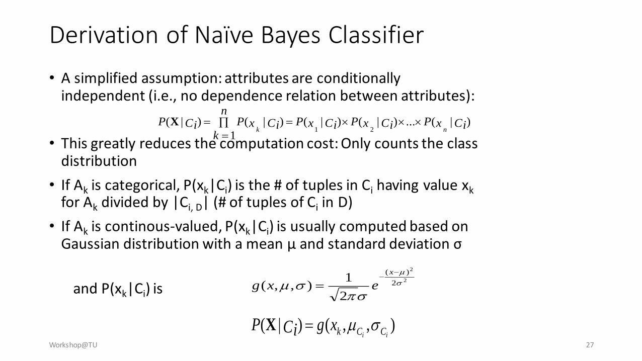
Derivation of Naïve Bayes Classifier
• A simplified assumption: attributes are conditionally independent (i.e., no dependence relation between attributes):
• This greatly reduces the computation cost: Only counts the class distribution
• If Ak is categorical, P(xk|Ci) is the # of tuples in Ci having value xk
for Ak divided by |Ci, D| (# of tuples of Ci in D)
• If Ak is continous-valued, P(xk|Ci) is usually computed based on Gaussian distribution with a mean μ and standard deviation σ
and P(xk|Ci) is
)|(...)|()|(
1
)|()|(21
CixPCixPCixPn
kCixPCiP
nk
X
2
2
2
)(
2
1),,(
x
exg
),,()|(ii CCkxgCiP X
Workshop@TU 28
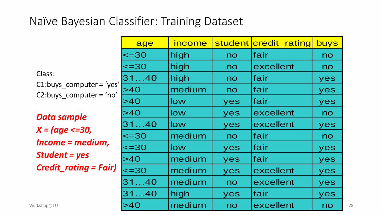
Naïve Bayesian Classifier: Training Dataset
Class:
C1:buys_computer = ‘yes’
C2:buys_computer = ‘no’
Data sample
X = (age <=30,
Income = medium,
Student = yes
Credit_rating = Fair)
age income student credit_rating buys
<=30 high no fair no
<=30 high no excellent no
31…40 high no fair yes
>40 medium no fair yes
>40 low yes fair yes
>40 low yes excellent no
31…40 low yes excellent yes
<=30 medium no fair no
<=30 low yes fair yes
>40 medium yes fair yes
<=30 medium yes excellent yes
31…40 medium no excellent yes
31…40 high yes fair yes
>40 medium no excellent no
Workshop@TU 29
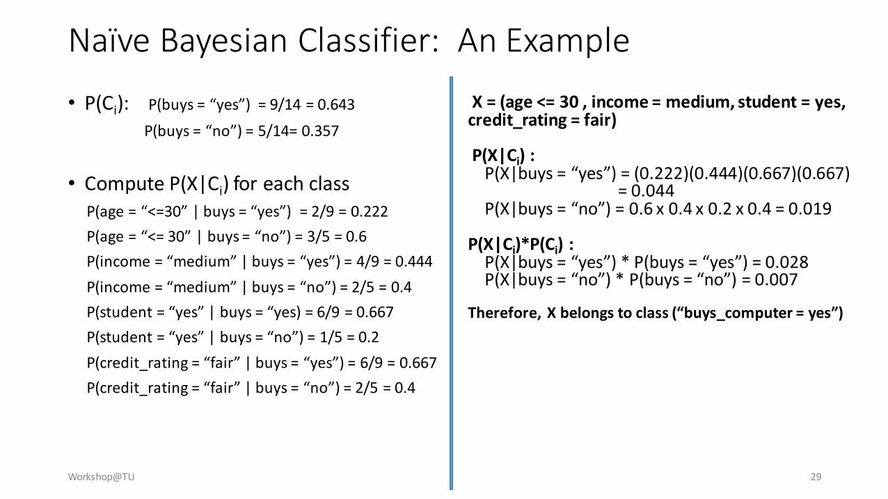
Naïve Bayesian Classifier: An Example
• P(Ci): P(buys = “yes”) = 9/14 = 0.643
P(buys = “no”) = 5/14= 0.357
• Compute P(X|Ci) for each classP(age = “<=30” | buys = “yes”) = 2/9 = 0.222
P(age = “<= 30” | buys = “no”) = 3/5 = 0.6
P(income = “medium” | buys = “yes”) = 4/9 = 0.444
P(income = “medium” | buys = “no”) = 2/5 = 0.4
P(student = “yes” | buys = “yes) = 6/9 = 0.667
P(student = “yes” | buys = “no”) = 1/5 = 0.2
P(credit_rating = “fair” | buys = “yes”) = 6/9 = 0.667
P(credit_rating = “fair” | buys = “no”) = 2/5 = 0.4
X = (age <= 30 , income = medium, student = yes, credit_rating = fair)
P(X|Ci) :P(X|buys = “yes”) = (0.222)(0.444)(0.667)(0.667)
= 0.044P(X|buys = “no”) = 0.6 x 0.4 x 0.2 x 0.4 = 0.019
P(X|Ci)*P(Ci) :P(X|buys = “yes”) * P(buys = “yes”) = 0.028 P(X|buys = “no”) * P(buys = “no”) = 0.007
Therefore, X belongs to class (“buys_computer = yes”)

Workshop 4
• Apply Naïve Bayes to the previous datasets
Workshop@TU 30

Workshop@TU 31
4. Using IF-THEN Rules for Classification
• Represent the knowledge in the form of IF-THEN rules
R: IF age = youth AND student = yes THEN buys_computer = yes
• Rule antecedent/precondition vs. rule consequent
• Assessment of a rule: coverage and accuracy
• ncovers = # of tuples covered by R
• ncorrect = # of tuples correctly classified by R
coverage(R) = ncovers /|D| /* D: training data set */
accuracy(R) = ncorrect / ncovers
• If more than one rule is triggered, need conflict resolution
• Size ordering: assign the highest priority to the triggering rules that has the “toughest” requirement (i.e., with the most attribute test)
• Class-based ordering: decreasing order of prevalence or misclassification cost per class
• Rule-based ordering (decision list): rules are organized into one long priority list, according to some measure of rule quality or by experts
Workshop@TU 32
age?
student? credit rating?
<=30 >40
no yes yes
yes
31..40
fairexcellentyesno
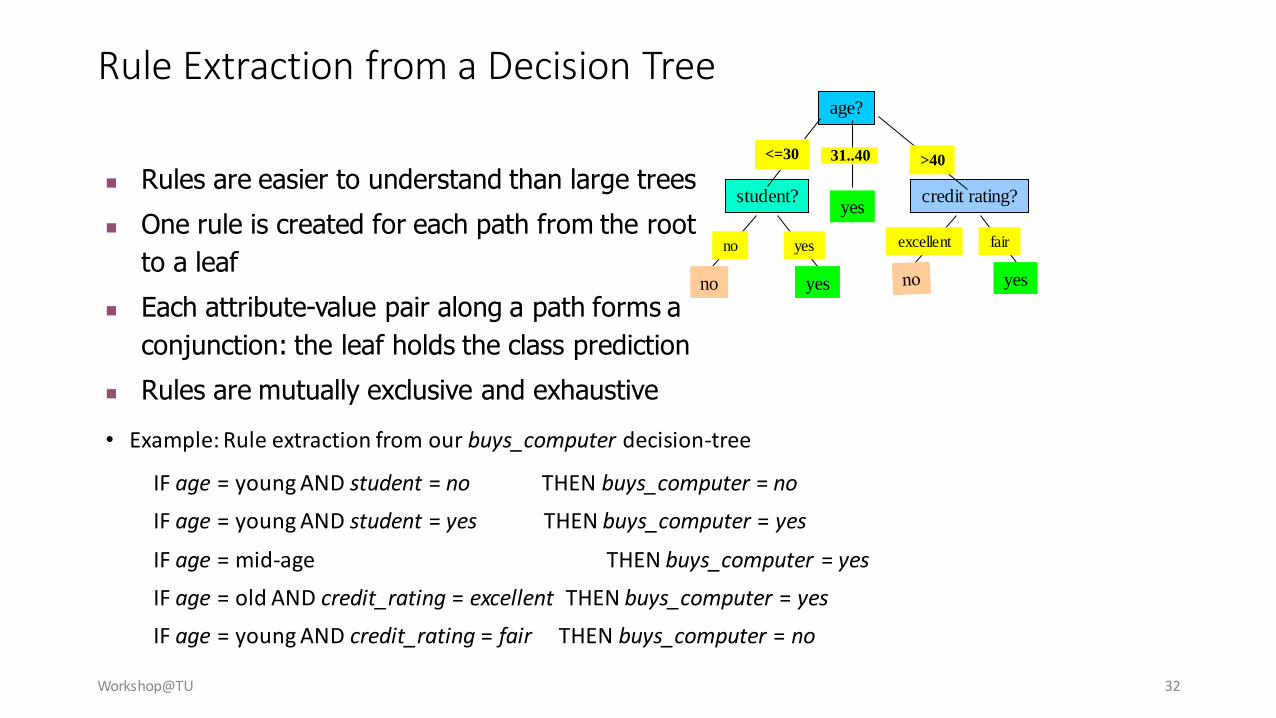
• Example: Rule extraction from our buys_computer decision-tree
IF age = young AND student = no THEN buys_computer = no
IF age = young AND student = yes THEN buys_computer = yes
IF age = mid-age THEN buys_computer = yes
IF age = old AND credit_rating = excellent THEN buys_computer = yes
IF age = young AND credit_rating = fair THEN buys_computer = no
Rule Extraction from a Decision Tree
Rules are easier to understand than large trees
One rule is created for each path from the root
to a leaf
Each attribute-value pair along a path forms a
conjunction: the leaf holds the class prediction
Rules are mutually exclusive and exhaustive

Workshop@TU 33
Learn-One-Rule Algorithm
X
Y
+ +
++
+
+
+
+ +
+
+ +
+

Workshop@TU 34
X
Y
+ +
++
+
+
+
+ +
+
+ +
+Y>C1
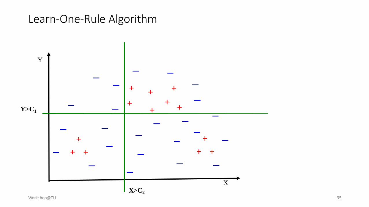
Learn-One-Rule Algorithm
Workshop@TU 35
X
Y
+ +
++
+
+
+
+ +
+
+ +
+Y>C1
X>C2
Learn-One-Rule Algorithm
Workshop@TU 3627
X
Y
+ +
++
+
+
+
+ +
+
+ +
+Y>C1
X>C2
Y<C3
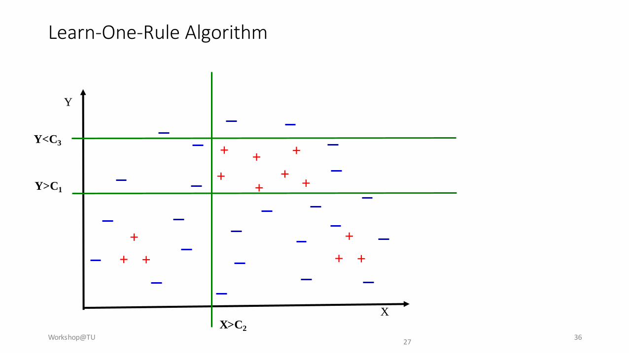
Learn-One-Rule Algorithm
Workshop@TU 37
X
Y
+ +
++
+
+
+
+ +
+
+ +
+Y>C1
X>C2
Y<C3
X<C4
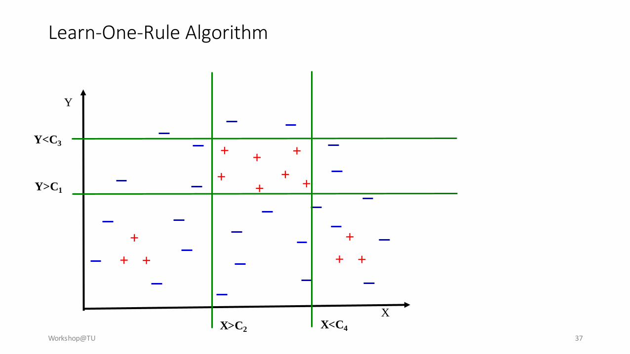
Learn-One-Rule Algorithm
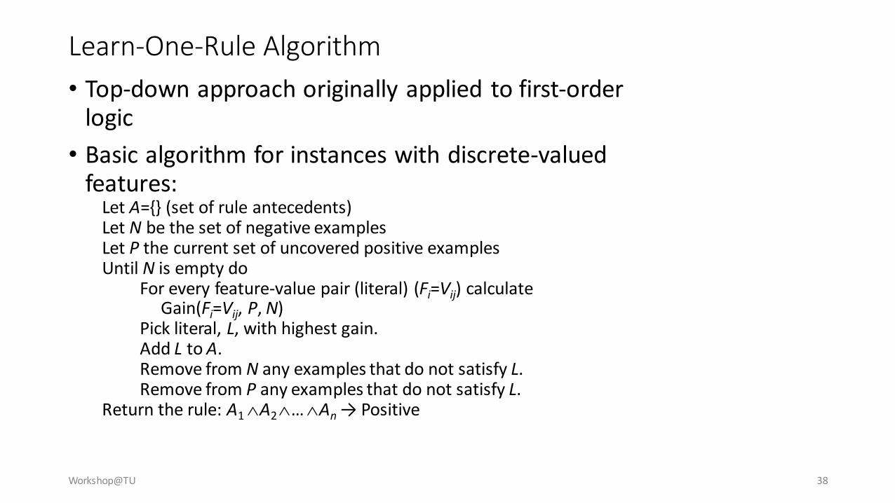
Workshop@TU 38
• Top-down approach originally applied to first-order logic
• Basic algorithm for instances with discrete-valued features:
Let A={} (set of rule antecedents)Let N be the set of negative examplesLet P the current set of uncovered positive examplesUntil N is empty do
For every feature-value pair (literal) (Fi=Vij) calculateGain(Fi=Vij, P, N)
Pick literal, L, with highest gain.Add L to A.Remove from N any examples that do not satisfy L.Remove from P any examples that do not satisfy L.
Return the rule: A1 A2 … An → Positive
Learn-One-Rule Algorithm
Workshop@TU 3941
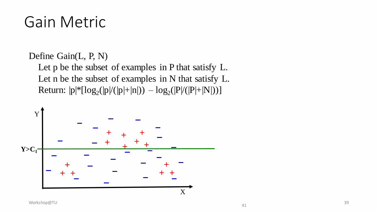
Gain Metric
Define Gain(L, P, N)
Let p be the subset of examples in P that satisfy L.
Let n be the subset of examples in N that satisfy L.
Return: |p|*[log2(|p|/(|p|+|n|)) – log2(|P|/(|P|+|N|))]
X
Y
+ +++
+
+
++ +
++ +
+Y>C1
Workshop 5
• Apply rule learner algorithms to the previous datasetsCompare results from datasets with/without discretization
Workshop@TU 40