Introduction to Data Models used in Geographic Information Systems

Miles Logsdonmlog@u.washington.edu

Garry Trudeau - Doonesbury

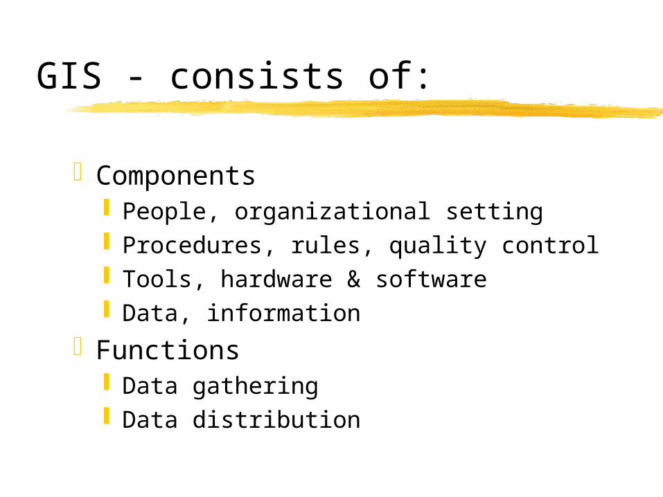
GIS - consists of:

Components People, organizational setting Procedures, rules, quality control Tools, hardware & software Data, information

Functions Data gathering Data distribution

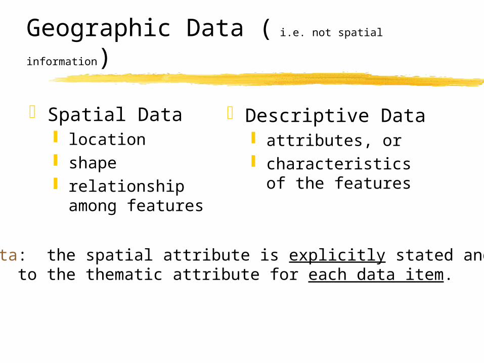
Geographic Data ( i.e. not spatial information)

Spatial Data location shape relationship among

features

Descriptive Data attributes, or characteristics of

the features

Spatial Data: the spatial attribute is explicitly stated and linked to the thematic attribute for each data item.

• Map Projection Properties

Map Projections – cont.

• Conformality, Shape is preserved

• Equaldistant

•Azimuths (directions)

•Scale

•Area

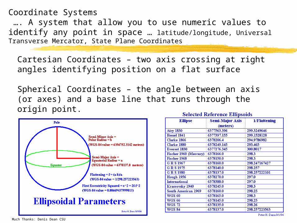
Coordinate Systems …. A system that allow you to use numeric values to identify any point in space … latitude/longitude, Universal Transverse Mercator, State Plane Coordinates

Cartesian Coordinates – two axis crossing at right angles identifying position on a flat surface

Spherical Coordinates – the angle between an axis (or axes) and a base line that runs through the origin point.

Much Thanks: Denis Dean CSU

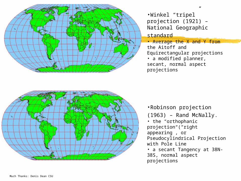
•Winkel “tripel” projection (1921) –

National Geographic standard • Average the X and Y from the Aitoff and Equirectangular projections• a modified planner, secant, normal aspect projections

•Robinson projection (1963) – Rand

McNally. • the “orthophanic projection (“right appearing”, or Pseudocylindrical Projection with Pole Line• a secant Tangency at 38N-38S, normal aspect projections

Much Thanks: Denis Dean CSU

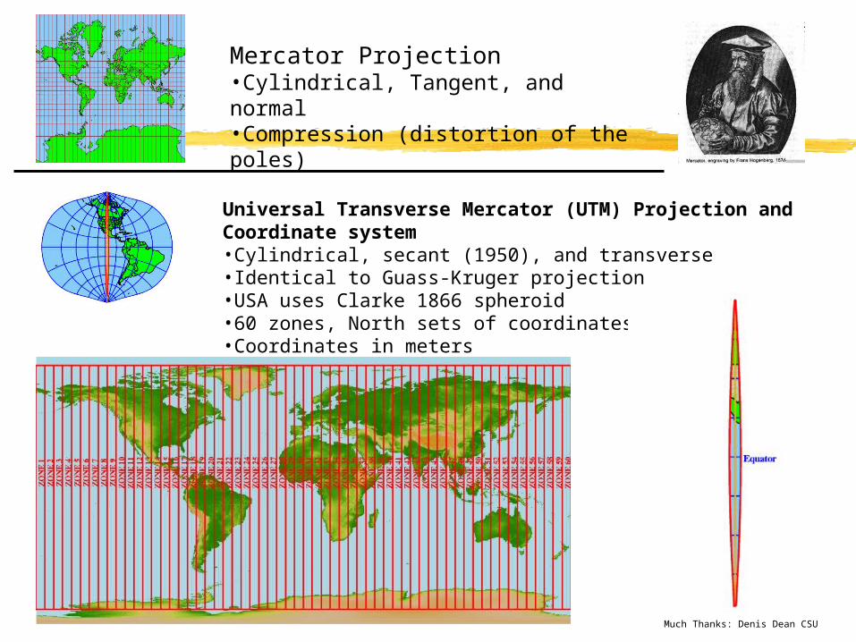
Mercator Projection•Cylindrical, Tangent, and normal•Compression (distortion of the poles)

Universal Transverse Mercator (UTM) Projection and Coordinate system•Cylindrical, secant (1950), and transverse•Identical to Guass-Kruger projection•USA uses Clarke 1866 spheroid•60 zones, North sets of coordinates all positive•Coordinates in meters

Much Thanks: Denis Dean CSU

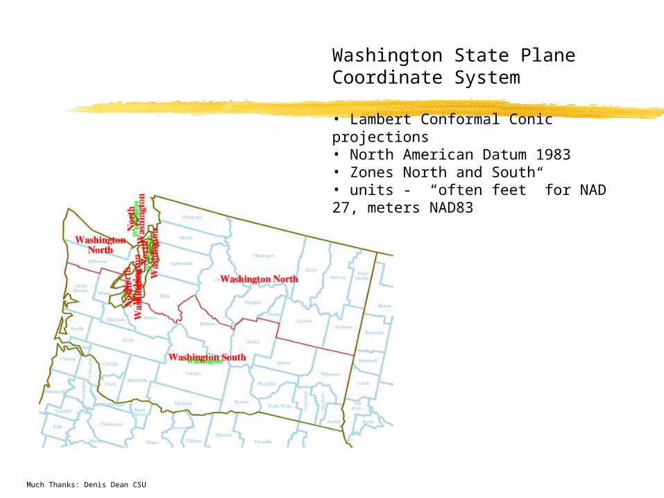
Washington State Plane Coordinate System

• Lambert Conformal Conic projections• North American Datum 1983• Zones North and South• units - “often feet” for NAD 27, meters NAD83

Much Thanks: Denis Dean CSU

Spatial Information

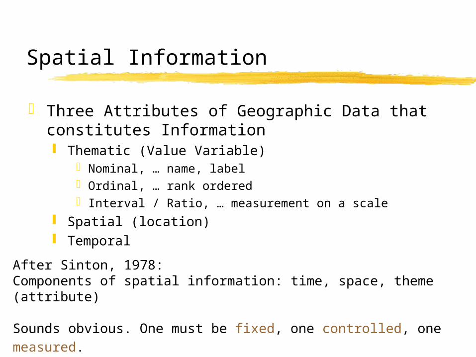
Three Attributes of Geographic Data that constitutes Information Thematic (Value Variable)

Nominal, … name, label Ordinal, … rank ordered Interval / Ratio, … measurement on a scale

Spatial (location) Temporal

After Sinton, 1978:Components of spatial information: time, space, theme (attribute)

Sounds obvious. One must be fixed, one controlled, one measured.

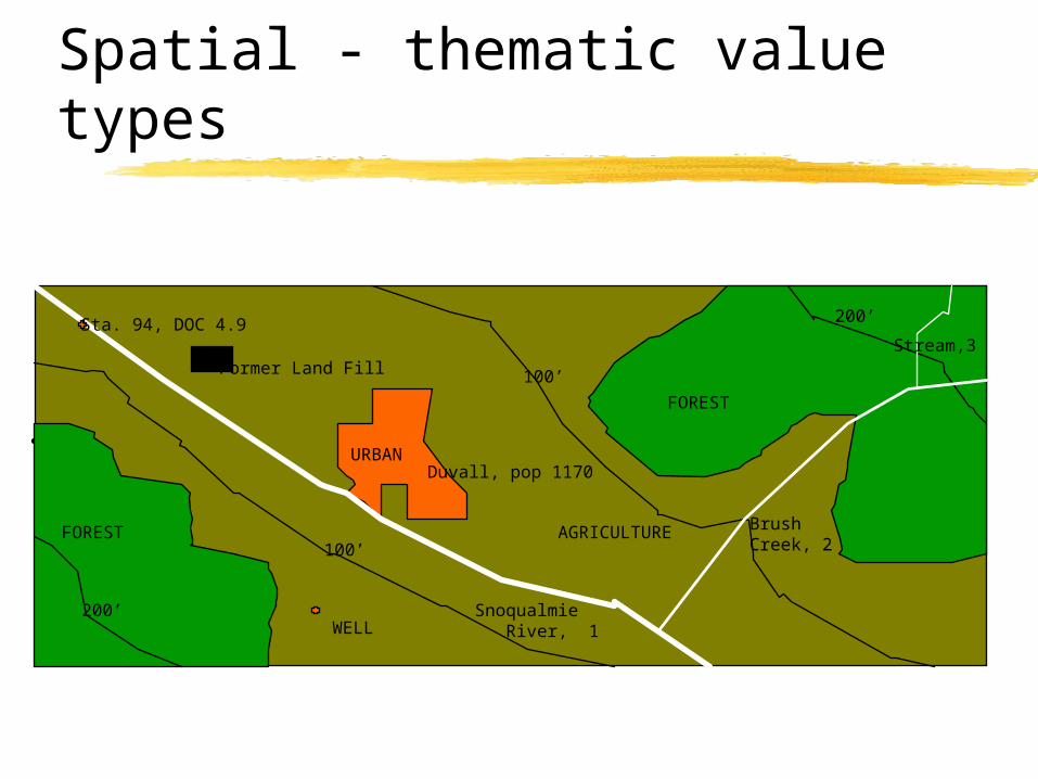
Spatial - thematic value types

Sta. 94, DOC 4.9

WELL200’

100’

100’

200’

Former Land Fill

URBANDuvall, pop 1170

FOREST

FOREST

AGRICULTURE

Snoqualmie River, 1

BrushCreek, 2

Stream,3

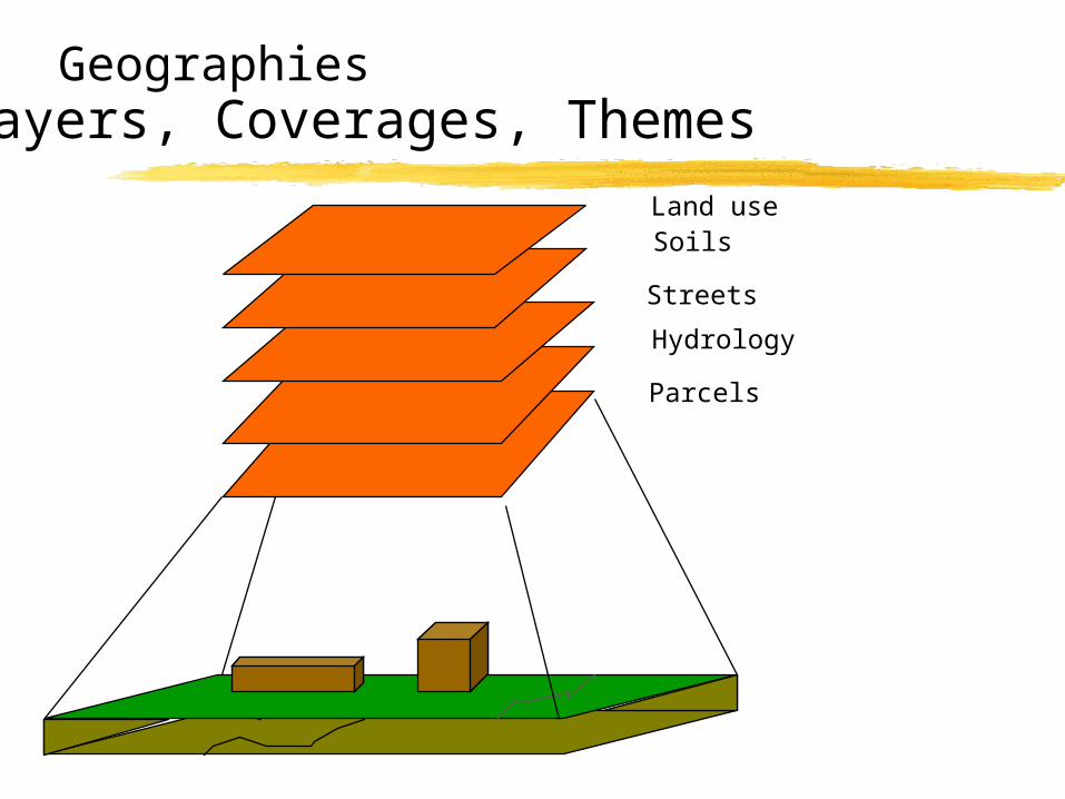
GeographiesLayers, Coverages, Themes

Land useSoils

Streets

Hydrology

Parcels

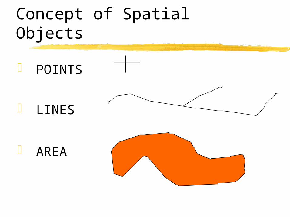
Concept of Spatial Objects

POINTS

LINES

AREA

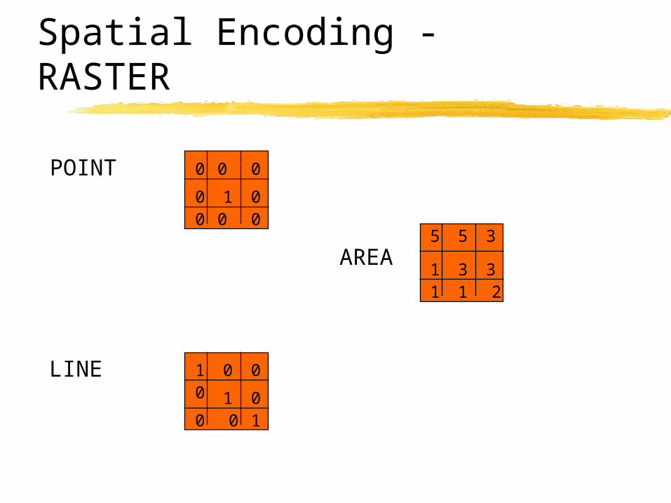
Spatial Encoding - RASTER

0 00

00 0 0

01

POINT

1

0

1

11

0 0

00

0

5 5 3

3311 2

LINE

AREA

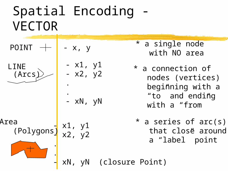
Spatial Encoding - VECTOR

POINT - x, y

LINE - x1, y1- x2, y2..- xN, yN

Area (Polygons)

- x1, y1- x2, y2..- xN, yN (closure Point)

* a single node with NO area

* a connection of nodes (vertices) beginning with a “to” and ending with a “from”

(Arcs)

* a series of arc(s) that close around a “label” point

Vector - Topology

Object Spatial Descriptive

1

2 3

45

15

1211

10

123

x1,y1x2,y2x3,y3

123

12

12

12

12

VAR1 VAR2

VAR1 VAR2

VAR1 VAR2

Fnode Tnode x1y1, x2y2

1 2 xxyy, xxyy2 3 xxyy,xxyy

10, 11, 12, 1510, …….

1

2 3

1

2

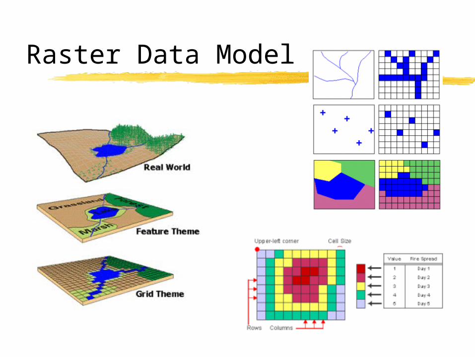
Raster Data Model

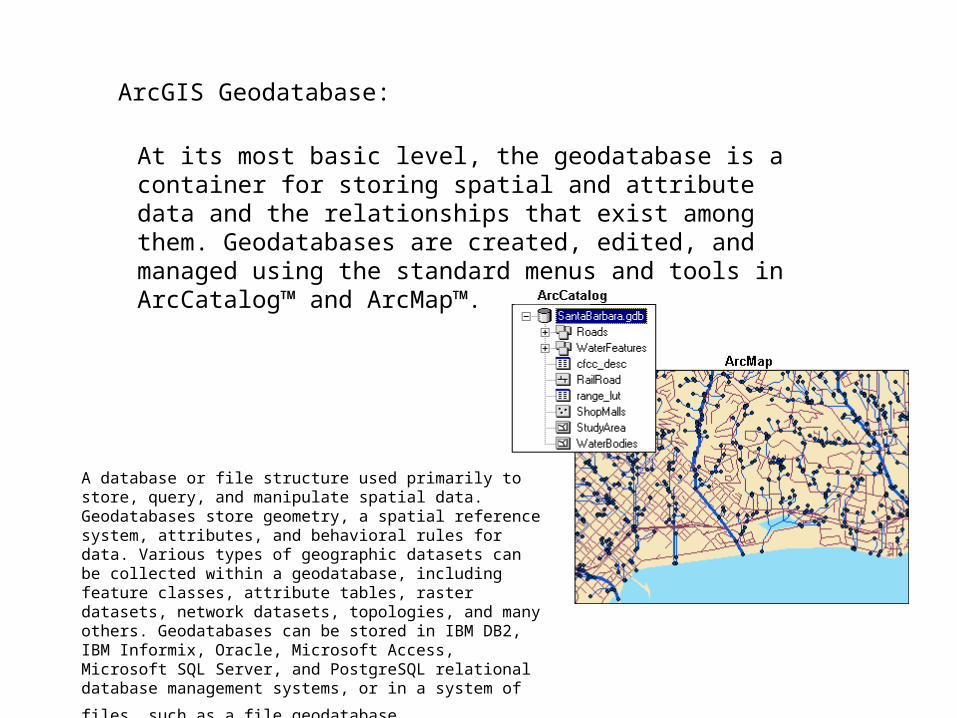
At its most basic level, the geodatabase is a container for storing spatial and attribute data and the relationships that exist among them. Geodatabases are created, edited, and managed using the standard menus and tools in ArcCatalog™ and ArcMap™.

A database or file structure used primarily to store, query, and manipulate spatial data. Geodatabases store geometry, a spatial reference system, attributes, and behavioral rules for data. Various types of geographic datasets can be collected within a geodatabase, including feature classes, attribute tables, raster datasets, network datasets, topologies, and many others. Geodatabases can be stored in IBM DB2, IBM Informix, Oracle, Microsoft Access, Microsoft SQL Server, and PostgreSQL relational database management systems, or in a system of

files, such as a file geodatabase.

ArcGIS Geodatabase:

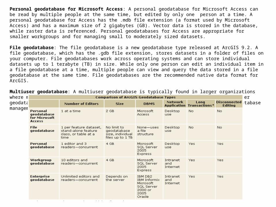
Personal geodatabase for Microsoft Access: A personal geodatabase for Microsoft Access can be read by multiple people at the same time, but edited by only one person at a time. A personal geodatabase for Access has the .mdb file extension (a format used by Microsoft Access) and has a maximum size of 2 gigabytes (GB). Vector data is stored in the database, while raster data is referenced. Personal geodatabases for Access are appropriate for smaller workgroups and for managing small to moderately sized datasets. File geodatabase: The file geodatabase is a new geodatabase type released at ArcGIS 9.2. A file geodatabase, which has the .gdb file extension, stores datasets in a folder of files on your computer. File geodatabases work across operating systems and can store individual datasets up to 1 terabyte (TB) in size. While only one person can edit an individual item in a file geodatabase at a time, multiple people can view and query the data stored in a file geodatabase at the same time. File geodatabases are the recommended native data format for ArcGIS. Multiuser geodatabase: A multiuser geodatabase is typically found in larger organizations where multiple users need to view and edit the GIS database at the same time. Multiuser geodatabases support versions and replication and require ArcSDE technology and a database management system (DBMS) such as Informix, Microsoft SQL Server, or Oracle.

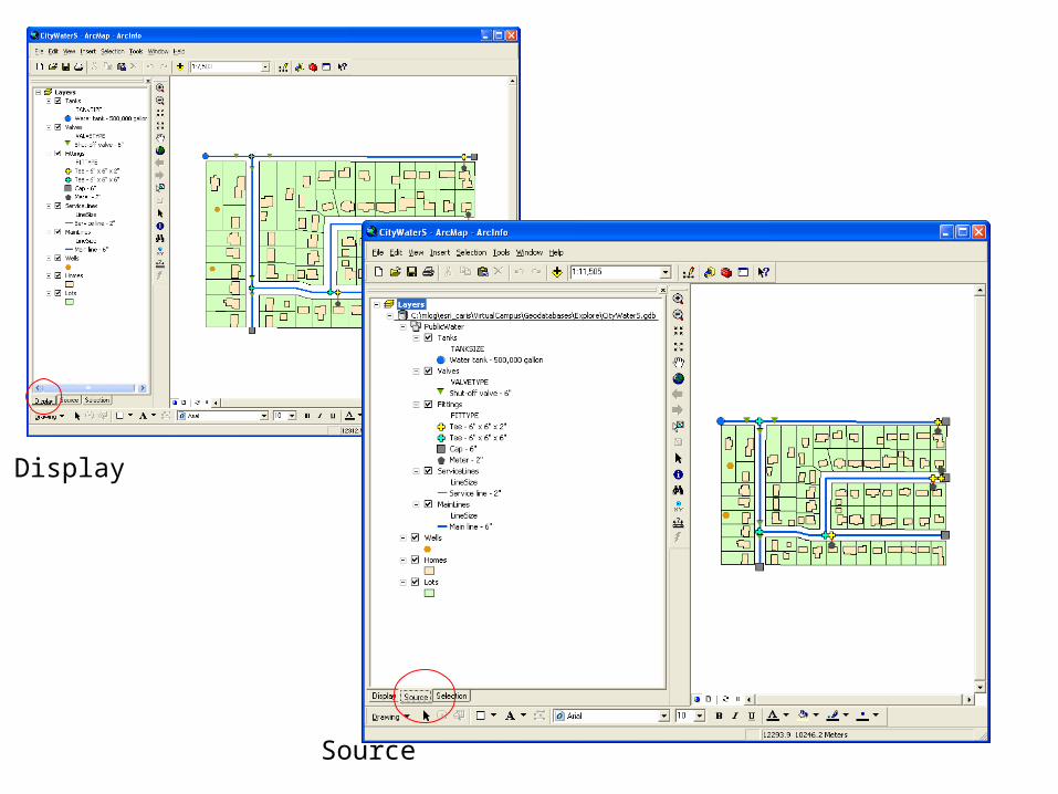
Display

Source

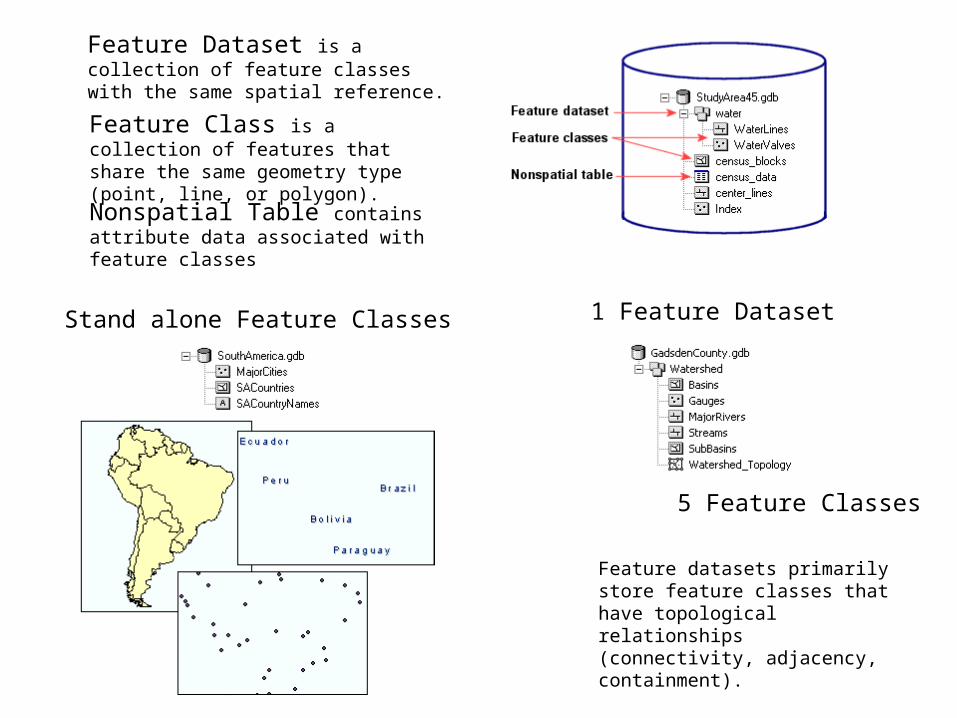
Feature Dataset is a collection of feature classes with the same spatial reference.

Feature Class is a collection of features that share the same geometry type (point, line, or polygon).

Nonspatial Table contains attribute data associated with feature classes

Stand alone Feature Classes 1 Feature Dataset

5 Feature Classes

Feature datasets primarily store feature classes that have topological relationships (connectivity, adjacency, containment).

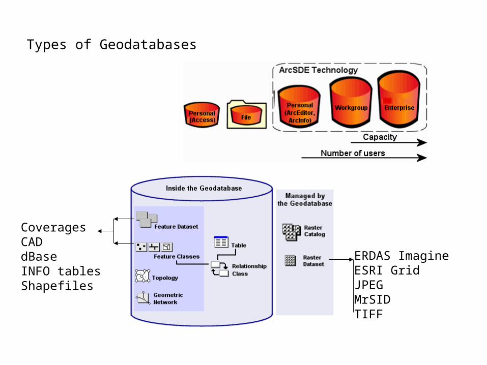
Types of Geodatabases

ERDAS ImagineESRI GridJPEGMrSIDTIFF

CoveragesCADdBaseINFO tablesShapefiles

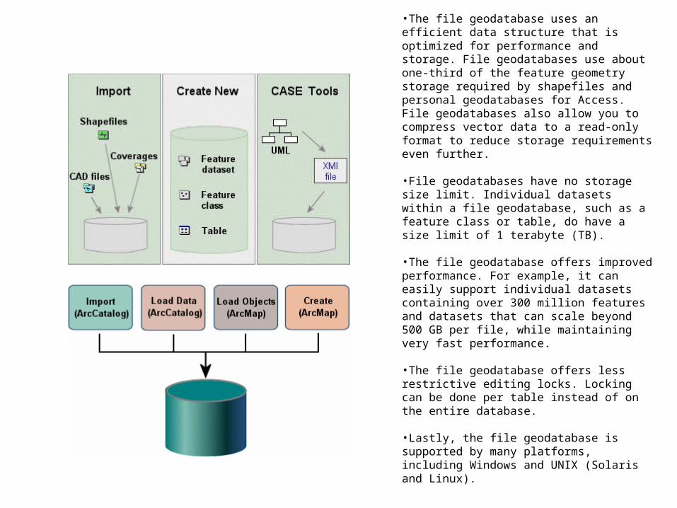
•The file geodatabase uses an efficient data structure that is optimized for performance and storage. File geodatabases use about one-third of the feature geometry storage required by shapefiles and personal geodatabases for Access. File geodatabases also allow you to compress vector data to a read-only format to reduce storage requirements even further.

•File geodatabases have no storage size limit. Individual datasets within a file geodatabase, such as a feature class or table, do have a size limit of 1 terabyte (TB).

•The file geodatabase offers improved performance. For example, it can easily support individual datasets containing over 300 million features and datasets that can scale beyond 500 GB per file, while maintaining very fast performance.

•The file geodatabase offers less restrictive editing locks. Locking can be done per table instead of on the entire database.

•Lastly, the file geodatabase is supported by many platforms, including Windows and UNIX (Solaris and Linux).

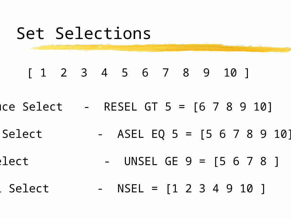
Set Selections

Reduce Select - RESEL GT 5 = [6 7 8 9 10]

Add Select - ASEL EQ 5 = [5 6 7 8 9 10]

Unselect - UNSEL GE 9 = [5 6 7 8 ]

Null Select - NSEL = [1 2 3 4 9 10 ]

[ 1 2 3 4 5 6 7 8 9 10 ]

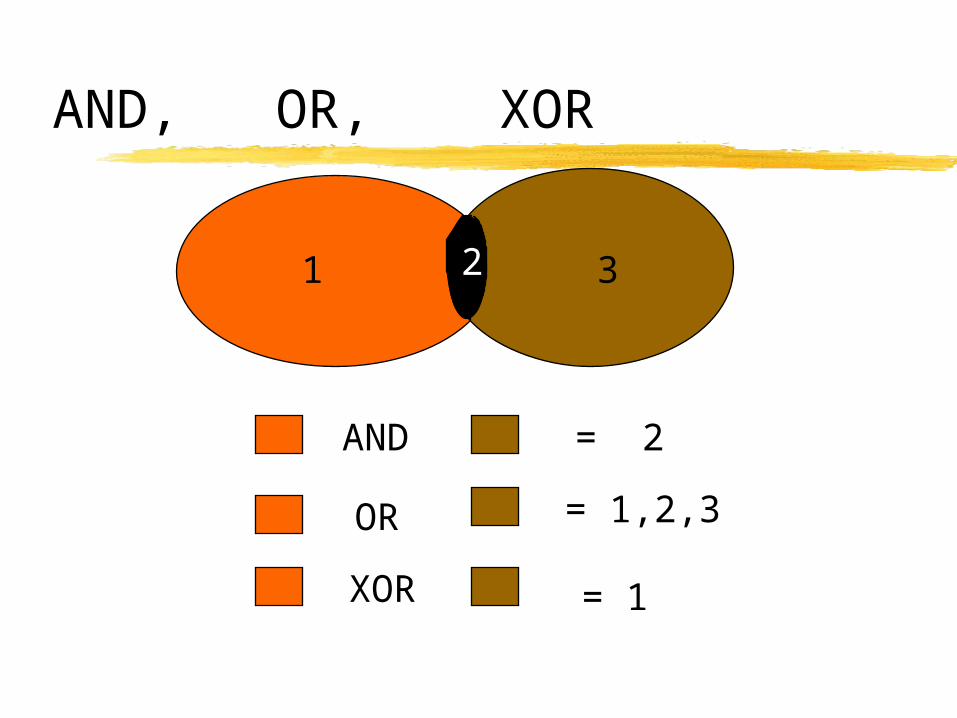
AND, OR, XOR

1 2 32

AND = 2

OR

XOR

= 1,2,3

= 1

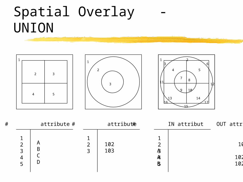
Spatial Overlay - UNION

1

2 3

4 5

1

2

3

1 23

4 5

6

78

9 10

1112

13 14

1516 17

12345

# attribute

123

# attribute

12345

# IN attribut OUT attribute

ABCD

102103

102 A A 102 B 102

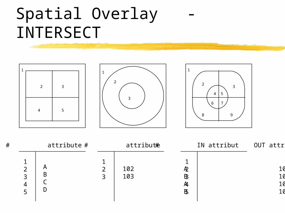
Spatial Overlay - INTERSECT

1

2 3

4 5

1

2

3

1

12345

# attribute

123

# attribute

12345

# IN attribut OUT attribute

ABCD

102103

A 102 B 102 A 103 B 103

23

4 5

6 7

8 9

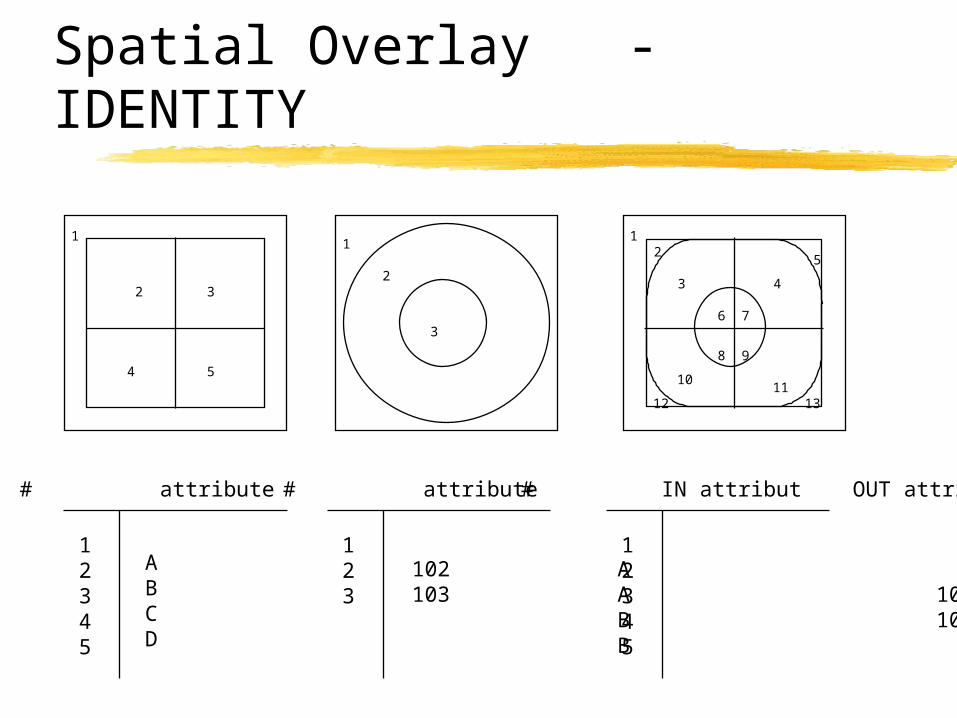
Spatial Overlay - IDENTITY

1

2 3

4 5

1

2

3

1

12345

# attribute

123

# attribute

12345

# IN attribut OUT attribute

ABCD

102103

A A 102 B 103 B

2

3 4

5

6 7

8 9

1011

12 13

Spatial Poximity - BUFFER

Constant Width

Variable Width

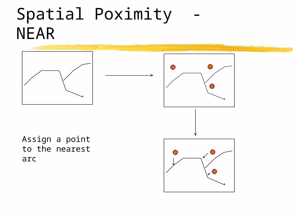
Spatial Poximity - NEAR

Assign a point to the nearest arc

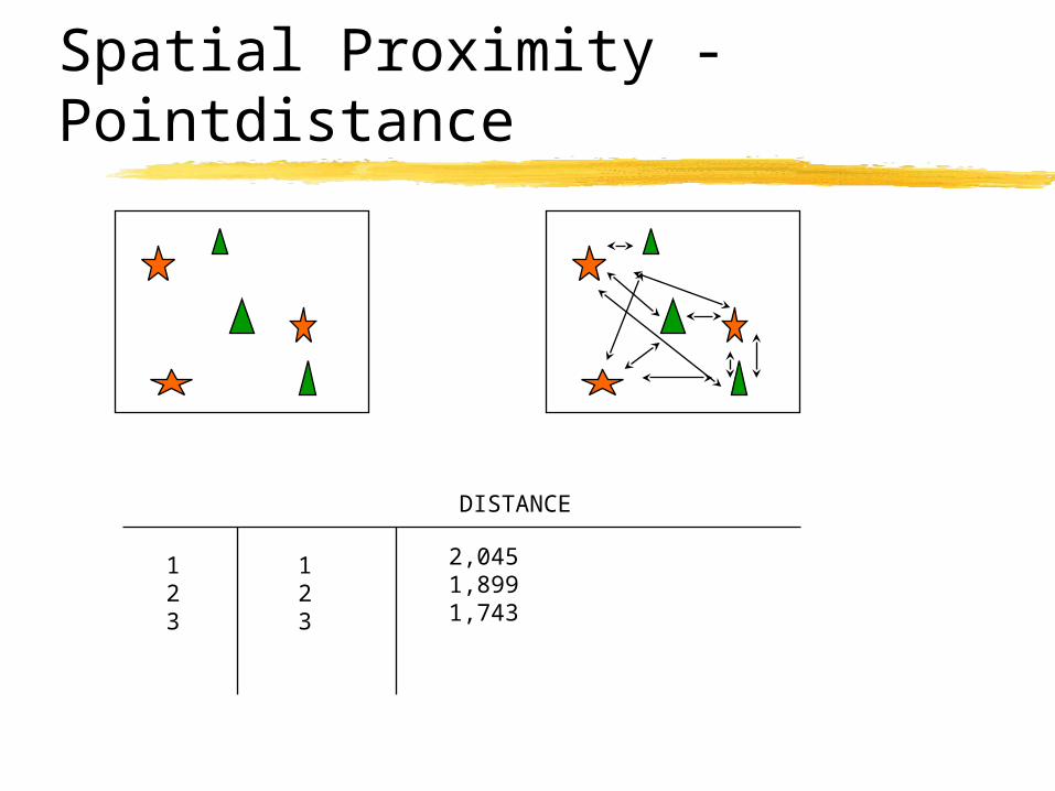
Spatial Proximity - Pointdistance

123

123

2,0451,8991,743

DISTANCE

Spatial Proximity - Thiessen Polygons

Map Algebra

In a raster GIS, cartographic modeling is also named Map Algebra.

Mathematical combinations of raster layers several types of functions: • Local functions • Focal functions • Zonal functions • Global functions

Functions can be applied to one or multiple layers

Local Function

Sometimes called layer functions -

Work on every single cell in a raster layer

•Cells are processed without reference to surrounding cells

•Operations can be arithmetic, trigonometric, exponential, logical or logarithmic functions

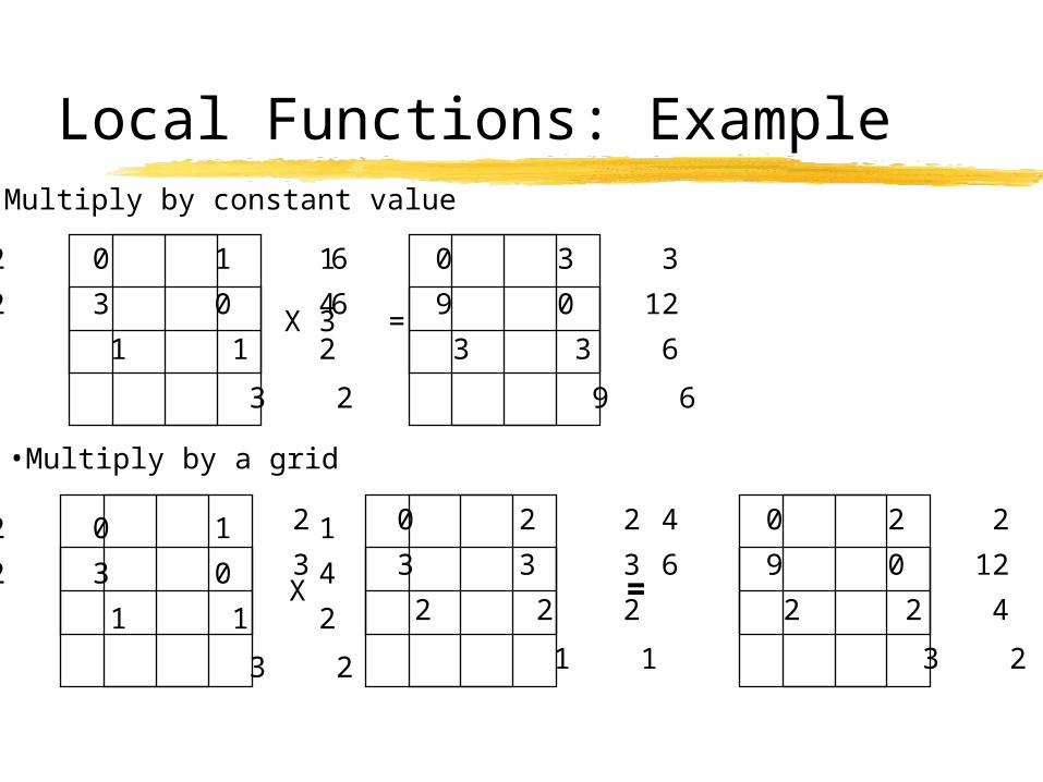
Local Functions: Example•Multiply by constant value

X 3 =

•Multiply by a grid

X =

2 0 1 1

2 3 0 4

1 1 2

3 2

2 0 1 1

2 3 0 4

1 1 2

3 2

6 0 3 3

6 9 0 12

3 3 6

9 6

2 0 2 2

3 3 3 3

2 2 2

1 1

4 0 2 2

6 9 0 12

2 2 4

3 2

Focal Function

Focal functions process cell data depending on the values of neighbouring cells

We define a ‘kernel’ to use as the neighbourhood •for example, 2x2, 3x3, 4x4 cells

Types of focal functions might be: •focal sum, •focal mean, •focal max, •focal min, •focal range

Focal Function: Examples

2 0 1 1

2 3 0 4

2 1 1 2

2 3 3 2

2 0 1 1

2 3 0 4

4 2 2 3

1 1 3 2

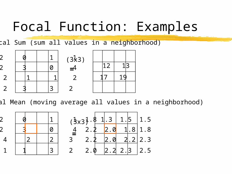
•Focal Sum (sum all values in a neighborhood)

=

=

•Focal Mean (moving average all values in a neighborhood)

1.8 1.3 1.5 1.5

2.2 2.0 1.8 1.8

2.2 2.0 2.2 2.3

2.0 2.2 2.3 2.5

(3x3)

(3x3) 12 13

17 19

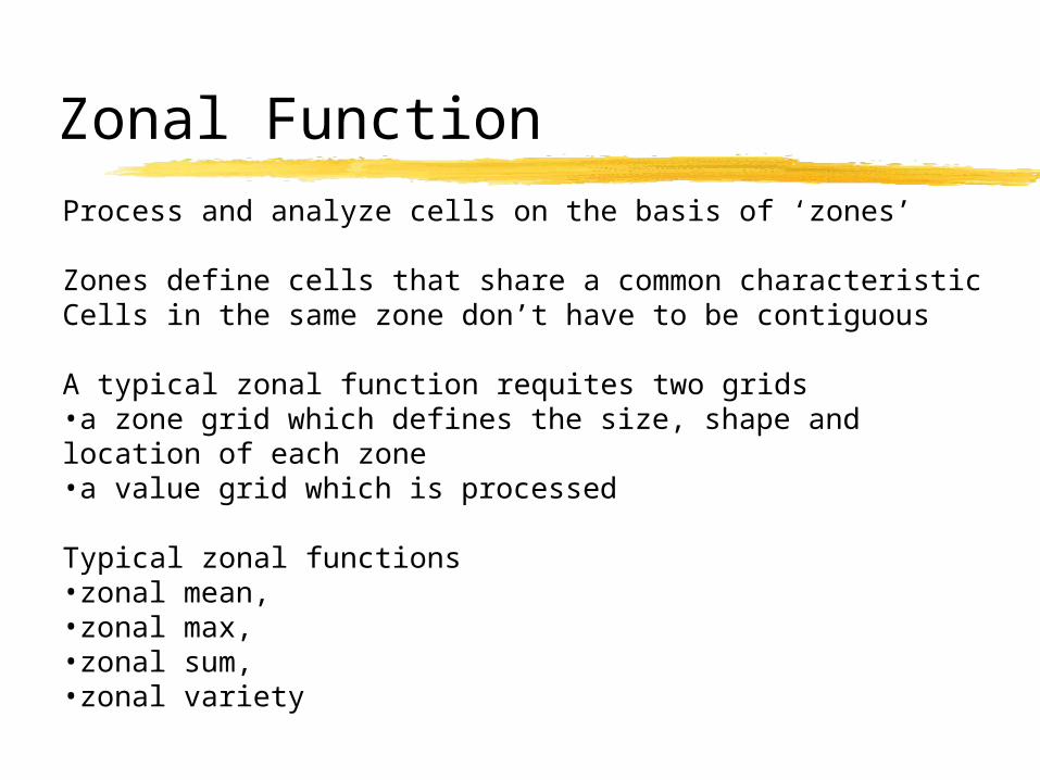
Zonal FunctionProcess and analyze cells on the basis of ‘zones’

Zones define cells that share a common characteristic Cells in the same zone don’t have to be contiguous

A typical zonal function requites two grids •a zone grid which defines the size, shape and location of each zone •a value grid which is processed

Typical zonal functions •zonal mean, •zonal max, •zonal sum, •zonal variety

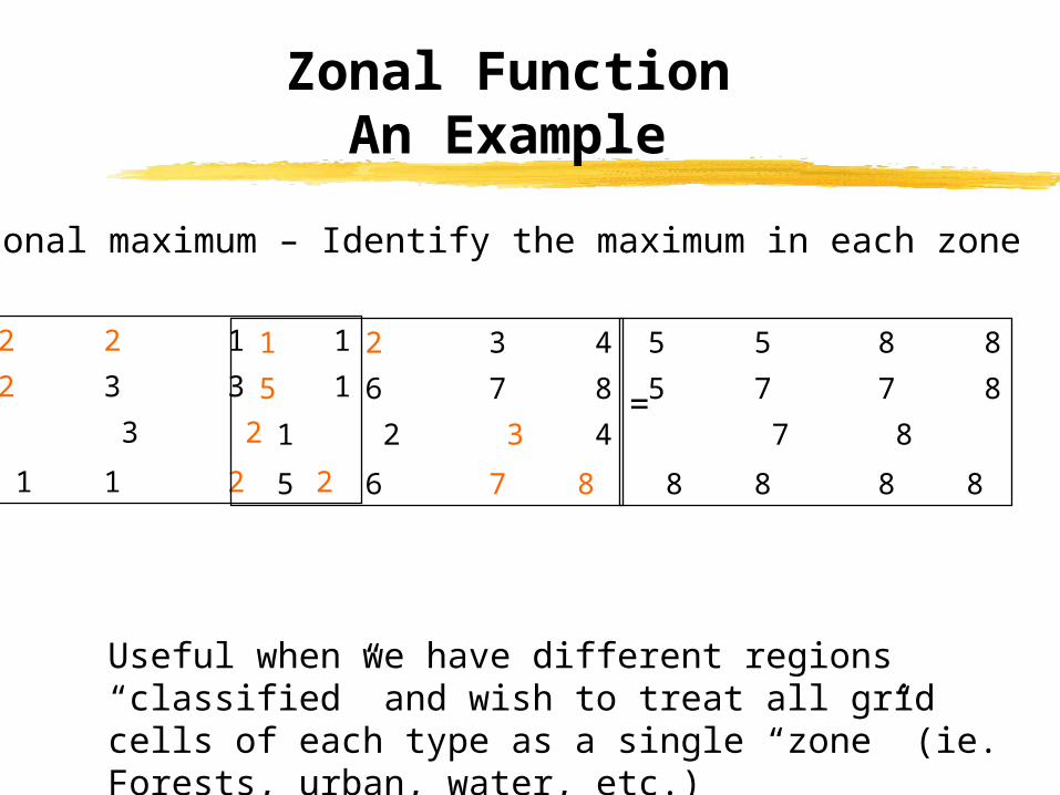
Zonal FunctionAn Example

•Zonal maximum – Identify the maximum in each zone

Useful when we have different regions “classified” and wish to treat all grid cells of each type as a single “zone” (ie. Forests, urban, water, etc.)

2 2 1 1

2 3 3 1

3 2

1 1 2 2

1 2 3 4

5 6 7 8

1 2 3 4

5 6 7 8

5 5 8 8

5 7 7 8

7 8

8 8 8 8

=

Global function

In global functions -

•The output value of each cell is a function of the entire grid

•Typical global functions are distance measures, flow directions, or weighting measures.

•Useful when we want to work out how cells ‘relate’ to each other

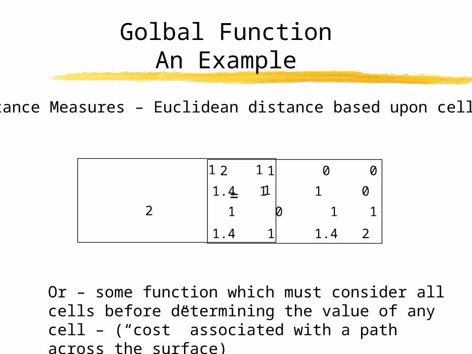
Golbal FunctionAn Example

•Distance Measures – Euclidean distance based upon cell size

Or – some function which must consider all cells before determining the value of any cell – (“cost” associated with a path across the surface)

1 1

1

2

2 1 0 0

1.4 1 1 0

1 0 1 1

1.4 1 1.4 2

=

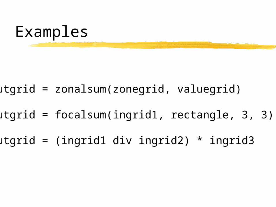
Examples

outgrid = zonalsum(zonegrid, valuegrid)

outgrid = focalsum(ingrid1, rectangle, 3, 3)

outgrid = (ingrid1 div ingrid2) * ingrid3

Spatial Modeling

Spatial modeling is analytical procedures applied with a GIS. Spatial modeling uses geographic data to attempt to describe, simulate or predict a real-world problem or system.

There are three categories of spatial modeling functions that can be applied to geographic features within a GIS: •geometric models, such as calculating the Euclidean distance between features, •coincidence models, such as topological overlay; •adjacency models (pathfinding, redistricting, and allocation)

All three model categories support operations on spatial data such as points, lines, polygons, tins, and grids. Functions are organized in a sequence of steps to derive the desired information for analysis.

The following references are excellent introductions to modeling in GIS:Goodchild, Parks, and Stegaert. Environmental Modeling with GIS. Oxford University Press, 1993.Tomlin, Dana C. Geographic Information Systems and Catograhic Modeling. Prentice Hall, 1990.