introduction to deep learning - ingegneria...
TRANSCRIPT

Sapienza University of Rome, Italy
University of Rome “La Sapienza”
Dep. of Computer, Control and Management Engineering A. Ruberti
Introduction to Deep Learning
Valsamis Ntouskos
ALCOR Lab
Valsamis Ntouskos (ALCOR Lab) Introduction to Deep Learning 1 / 39

Sapienza University of Rome, Italy
Overview
Linear Classification
Logistic Regression
Linear Regression
Deep Feedforward Networks
Training DFNs
Activation Function
Regularization
Valsamis Ntouskos (ALCOR Lab) Introduction to Deep Learning 2 / 39

Sapienza University of Rome, Italy
Linear Models for Classification
Learning a function f : X → Y , with ...
X ⊆ <n
Y = {C1, . . . ,Ck}
assuming linearly separable data.
Valsamis Ntouskos (ALCOR Lab) Introduction to Deep Learning 3 / 39

Sapienza University of Rome, Italy
Linearly separable data
Instances in a data set are linearly separable iff it exists a hyperplane thatdivide the instance space into two regions such that differently classifiedinstances are separated.
Valsamis Ntouskos (ALCOR Lab) Introduction to Deep Learning 4 / 39

Sapienza University of Rome, Italy
Discriminant functions
Linear discriminant function
y : X → {C1, . . . ,CK}
Two classes:y(x) = wTx + w0
Multi classes:yk(x) = wT
k x + wk0
Valsamis Ntouskos (ALCOR Lab) Introduction to Deep Learning 5 / 39

Sapienza University of Rome, Italy
Linear Classification
−4 −2 0 2 4 6 8
−8
−6
−4
−2
0
2
4
Valsamis Ntouskos (ALCOR Lab) Introduction to Deep Learning 6 / 39

Sapienza University of Rome, Italy
Basis functions
x1
x2
−1 0 1
−1
0
1
φ1
φ2
0 0.5 1
0
0.5
1
Valsamis Ntouskos (ALCOR Lab) Introduction to Deep Learning 7 / 39

Sapienza University of Rome, Italy
Logistic Regression
Consider first the case of two classes.
Find the conditional probability:
P(C1|x) =P(x|C1)P(C1)
P(x|C1)p(C1) + P(x|C2)p(C2)
=1
1 + exp(−α)= σ(α).
with:
α = ln P(x|C1)P(C1)P(x|C2)P(C2)
and
σ(α) = 11+exp(−α) the sigmoid function.
Valsamis Ntouskos (ALCOR Lab) Introduction to Deep Learning 8 / 39

Sapienza University of Rome, Italy
Logistic Regression
Assume P(x|Ci ) ∼ N (x|µi ,Σ) - same covariance matrix
we get:
P(C1|x) = σ(wTx + w0),
Multiclass logistic regression
p(Ck |φ) = yk(φ) =exp(ak)∑j exp(aj)︸ ︷︷ ︸softmax
,with ak = wTk φ
Valsamis Ntouskos (ALCOR Lab) Introduction to Deep Learning 9 / 39

Sapienza University of Rome, Italy
Linear Regression
Goal: Estimate the value t of a continuous function at x based on adataset D composed of N observations {xn}, where n = 1, . . . ,N,together with the corresponding target values {tn}.
Ideally:t = y(x,w)
Valsamis Ntouskos (ALCOR Lab) Introduction to Deep Learning 10 / 39
Sapienza University of Rome, Italy
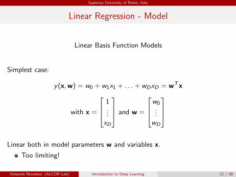
Linear Regression - Model
Linear Basis Function Models
Simplest case:
y(x,w) = w0 + w1x1 + . . .+ wDxD = wTx
with x =
1...xD
and w =
w0...
wD
Linear both in model parameters w and variables x.
Too limiting!
Valsamis Ntouskos (ALCOR Lab) Introduction to Deep Learning 11 / 39

Sapienza University of Rome, Italy
Example - Line fitting
y = w1x1 + w0
−4 −3 −2 −1 0 1 2 3 4−3
−2
−1
0
1
2
3
4
5
predictiontruth
Valsamis Ntouskos (ALCOR Lab) Introduction to Deep Learning 12 / 39
Sapienza University of Rome, Italy
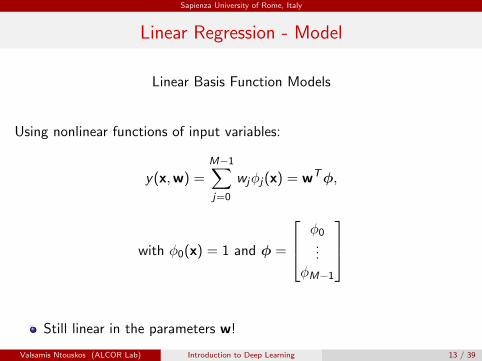
Linear Regression - Model
Linear Basis Function Models
Using nonlinear functions of input variables:
y(x,w) =M−1∑j=0
wjφj(x) = wTφ,
with φ0(x) = 1 and φ =
φ0...
φM−1
Still linear in the parameters w!
Valsamis Ntouskos (ALCOR Lab) Introduction to Deep Learning 13 / 39

Sapienza University of Rome, Italy
Example - Polynomial curve fitting
y = w0 + w1x + w2x2 + . . .+ wMxM =
M∑j=0
wjxj
x
t
M = 0
0 1
−1
0
1
x
t
M = 1
0 1
−1
0
1
x
t
M = 3
0 1
−1
0
1
x
t
M = 9
0 1
−1
0
1
Valsamis Ntouskos (ALCOR Lab) Introduction to Deep Learning 14 / 39

Sapienza University of Rome, Italy
Linear Regression - Model
Examples of basis functions
−1 0 1−1
−0.5
0
0.5
1
−1 0 10
0.25
0.5
0.75
1
−1 0 10
0.25
0.5
0.75
1
Polynomial Radial Sigmoid / Tanh
Valsamis Ntouskos (ALCOR Lab) Introduction to Deep Learning 15 / 39

Sapienza University of Rome, Italy
Deep Feedforward Networks
Alternative names:
Feedforward Neural Networks
(Artificial) Neural Networks - (A)NNs
Multilayer Perceptrons - MLPs
Represent a parametric function
Suitable for tasks described as associating a vector to another vector
Valsamis Ntouskos (ALCOR Lab) Introduction to Deep Learning 16 / 39

Sapienza University of Rome, Italy
Deep Feedforward Networks
Goal: Estimate some function f ∗
Examples:
Classification y = f ∗(x) with x ∈ X and y ∈ {c1, . . . , cK}Regression y = f ∗(x) with x ∈ X and y ∈ R
Density estimation y = f ∗(x) with x ∈ X and∫X y = 1
Framework: Define y = f (x,θ) and learn parameters θ
Valsamis Ntouskos (ALCOR Lab) Introduction to Deep Learning 17 / 39

Sapienza University of Rome, Italy
Deep Feedforward Networks
Data: target values tn corresponding to given input variable values xnsuch that tn ≈ f ∗(xn)We use ≈ as the data may be affected by noise.
Objective:Learn θ such that f (x,θ) approximates as much as possible f ∗.Training based on a suitable cost (loss) function
Note: Dataset contains no target values about hidden units!
Valsamis Ntouskos (ALCOR Lab) Introduction to Deep Learning 18 / 39

Sapienza University of Rome, Italy
DFN - Terminology
Feedforward information flows from input to output without any loops
Networks f is a composition of elementary functions in an acyclic graph
Example:f (x) = f (3)(f (2)(f (1)(x,θ(1)),θ(2)),θ(3))
where:
f (m) the m-th layer of the network
and
θ(m) the corresponding parameters
Valsamis Ntouskos (ALCOR Lab) Introduction to Deep Learning 19 / 39

Sapienza University of Rome, Italy
DFN - Terminology
DFNs are chain structures
The length of the chain is the depth of the network
Final layer also called output layer
Name deep learning follows from the use of networks with a large numberof layers (large depth)
Valsamis Ntouskos (ALCOR Lab) Introduction to Deep Learning 20 / 39

Sapienza University of Rome, Italy
Deep Feedforward Networks
Draw inspiration from brain structures
Image from Isaac Changhau https://isaacchanghau.github.io
Hidden layer output can be seen as an array of unit (neuron) activationsbased on the connections with the previous units
Note: Only use some insights, they are not a model of the brain function!
Valsamis Ntouskos (ALCOR Lab) Introduction to Deep Learning 21 / 39

Sapienza University of Rome, Italy
Deep Feedforward Networks
Why DFNs?
Linear models cannot model interaction between input variables
Kernel methods require the choice of suitable kernels
use generic kernels e.g. RBF, polynomial, etc. (convex problem)
use hand-crafted kernels - application specific (convex problem)
Deep leaning:consider parametric mapping functions φ and learn their parameters(non-convex problem)
Model:y = f (x,θ,w) = φ(x,θ)Tw
Valsamis Ntouskos (ALCOR Lab) Introduction to Deep Learning 22 / 39

Sapienza University of Rome, Italy
Gradient-based learning
Learning remarks
Parameters found via gradient-based learning
Unit saturation can hinder learning
When units saturate gradient becomes very small
Suitable cost function and unit nonlinearities help to avoid saturation
Valsamis Ntouskos (ALCOR Lab) Introduction to Deep Learning 23 / 39

Sapienza University of Rome, Italy
Cost function
Model implicitly defines a conditional distribution p(t|x,θ)
Cost function:Typically choose the negative log-likelihood - Maximum likelihood principle
J(θ) = − ln(p(t|x))
Example:Assuming additive Gaussian noise we have
p(t|x) = N (t|f (x,θ), β−1I )
and hence
J(θ) =1
2(t− f (x,θ))2
Valsamis Ntouskos (ALCOR Lab) Introduction to Deep Learning 24 / 39

Sapienza University of Rome, Italy
Gradient Computation
Information flows forward throughthe network when computingnetwork output y from input x
To train the network we need tocompute the gradients with respectto the network parameters θ
The back-propagation or backpropalgorithm is used to propagategradient computation from the costthrough the whole network
Image by Y. LeCun
Valsamis Ntouskos (ALCOR Lab) Introduction to Deep Learning 25 / 39

Sapienza University of Rome, Italy
Gradient Computation
Goal: Compute the gradient of the cost function w.r.t. the parameters
∇θJ(θ)
Analytic computation of the gradient is straightforward
simple application of the chain rule
numerical evaluation can be expensive
Back-propagation is simple and inexpensive.
Remarks:
back-propagation is not a training algorithm
back-propagation is only used to compute the gradients
back-propagation is not specific to DFNs
Valsamis Ntouskos (ALCOR Lab) Introduction to Deep Learning 26 / 39

Sapienza University of Rome, Italy
Learning algorithms
Stochastic Gradient Descent (SGD)
SGD with momentum
Algorithms with adaptive learning rates
Valsamis Ntouskos (ALCOR Lab) Introduction to Deep Learning 27 / 39

Sapienza University of Rome, Italy
Stochastic Gradient Descent
Require: Learning rate ηRequire: Initial values of θk ← 1while stopping criterion not met do
Sample a subset (minibatch) {x(1), . . . , x(m)} of m examples from thedataset DCompute gradient estimate: g = 1
m∇θ∑
i L(f (x(i),θ), t(i))Apply update: θ ← θ − ηgk ← k + 1
end while
Note: η might change according to some rule through the iterations
Valsamis Ntouskos (ALCOR Lab) Introduction to Deep Learning 28 / 39

Sapienza University of Rome, Italy
Output units activation functions
Network output units determine also the cost function.Let h = f (x,θ) the output of the hidden layers.
RegressionLinear units: Identity activation function - no nonlinearity
y = W Th + b
Used to model a conditional Gaussian distribution
p(t|x) = N (t|y , β−1)
Maximum likelihood equivalent to minimizing mean squared error
Note: Linear units do not saturate!
Valsamis Ntouskos (ALCOR Lab) Introduction to Deep Learning 29 / 39

Sapienza University of Rome, Italy
Output units activation functions
Binary classificationSigmoid units: Sigmoid activation function
y = σ(wTh + b)
We have seen that the likelihood corresponds to a Bernoulli distributionHence:
J(θ) = − lnP(t|x)
= − lnσ(α)t(1− σ(α))1−t
= − lnσ((2t − 1)α)
= softplus((1− 2t)α),
with α = wTh + b.
Note: Unit saturates only when it gives the correct answer.If α has wrong sign softplus((1− 2t)α) ≈ |α| and dy
dα ≈ sign(α).Valsamis Ntouskos (ALCOR Lab) Introduction to Deep Learning 30 / 39

Sapienza University of Rome, Italy
Output units activation functions
− −10 5 0 5 100
2
4
6
8
10ζx()
The softplus function
Valsamis Ntouskos (ALCOR Lab) Introduction to Deep Learning 31 / 39

Sapienza University of Rome, Italy
Output units activation functions
Multiclass classificationSoftmax units: Softmax activation function
y = softmax(α)i =exp(αi )∑
j αj
Likelihood corresponds to a Multinomial distributionHence:
J(θ)i = − ln softmax(α)i = ln∑j
exp(αj)− αi
Note: ln∑
j exp(αj) ≈ ln exp(maxj(αj)) = maxj αj .If αi corresponds to the correct answer the derivative is small.Misclassifications give large derivatives.
Valsamis Ntouskos (ALCOR Lab) Introduction to Deep Learning 32 / 39

Sapienza University of Rome, Italy
Hidden units activation functions
Rectified Linear Units:
g(α) = max{0, α}.
Easy to optimize - similar to linear units
Not differentiable at 0 - does not cause problems in practice
Valsamis Ntouskos (ALCOR Lab) Introduction to Deep Learning 33 / 39

Sapienza University of Rome, Italy
Hidden unit activation functions
Valsamis Ntouskos (ALCOR Lab) Introduction to Deep Learning 34 / 39

Sapienza University of Rome, Italy
Hidden unit activation functions
Sigmoid and hyperbolic tangent:
g(α) = σ(α)
andg(α) = tanh(α)
Closely related as tanh(α) = 2σ(2α)− 1.
Remarks:
No logarithm at the output, the units saturate easily.
Gradient based learning is very slow.
Hyperbolic tangent gives larger gradients with respect to the sigmoid.
Valsamis Ntouskos (ALCOR Lab) Introduction to Deep Learning 35 / 39

Sapienza University of Rome, Italy
Activation functions overview
Image from Geron A. ”Hands-On Machine Learning with Scikit-Learn and TensorFlow”, O’Reilly 2017
Valsamis Ntouskos (ALCOR Lab) Introduction to Deep Learning 36 / 39

Sapienza University of Rome, Italy
Regularization
Early stopping:Stop iterations early to avoid overfitting to the training set of data
Valsamis Ntouskos (ALCOR Lab) Introduction to Deep Learning 37 / 39

Sapienza University of Rome, Italy
Regularization
Dropout: Randomly remove network units with some probability α
(a) Standard Neural Net (b) After applying dropout.
Image from Srivastava et al.. ”Dropout: A Simple Way to Prevent Neural Networks from Overfitting”
Valsamis Ntouskos (ALCOR Lab) Introduction to Deep Learning 38 / 39

Sapienza University of Rome, Italy
Regularization
With dropout
Without dropout
Image from Srivastava et al.. ”Dropout: A Simple Way to Prevent Neural Networks from Overfitting”
Valsamis Ntouskos (ALCOR Lab) Introduction to Deep Learning 39 / 39