introduction to differential algebraic equations · pdf fileintroduction to di erential...

Introduction to Differential Algebraic Equations

Dr. Abebe Geletu

Ilmenau University of TechnologyDepartment of Simulation and Optimal Processes (SOP)

Winter Semester 2011/12


TU Ilmenau

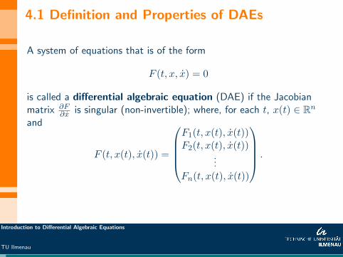
4.1 Definition and Properties of DAEs

A system of equations that is of the form

F (t, x, x) = 0

is called a differential algebraic equation (DAE) if the Jacobianmatrix ∂F

∂x is singular (non-invertible); where, for each t, x(t) ∈ Rn

and

F (t, x(t), x(t)) =

F1(t, x(t), x(t))F2(t, x(t), x(t))

...Fn(t, x(t), x(t))

.


TU Ilmenau

4.1 Definition and Properties of DAEs ...Example: The system

x1 − x1 + 1 = 0 (1)

x1x2 + 2 = 0 (2)

is a DAE. To see this, determine the Jacobian ∂F∂x of

F (t, x, x) =

(x1 − x1 + 1x1x2 + 2

)with x =

(x1x2

), so that

∂F

∂x=

(∂F1∂x1

∂F1∂x2

∂F2∂x1

∂F2∂x2

)=

(−1 0x2 0

), ( see that, det

(∂F

∂x

)= 0).

⇒ the Jacobian is a singular matrix irrespective of the values of x2.Observe that: in this example the derivative x2 does not appear.


TU Ilmenau

4.1 Definition and Properties of DAEs ...

Solving for x1 from the first equation x1 − x1 + 1 = 0 we getx1 = x1 + 1. Replace this for x1 in the second equation x1x2 + 2 = 0to wire the DAE in equations (23) & (23) equivalently as:

x1 = x1 + 1 (3)

(x1 + 1)x2 + 2 = 0 (4)

In this DAE:• equation (3) is a differential equation; while• equation (4) is an algebraic equation.⇒ There are several engineering applications that have such modelequations.


TU Ilmenau

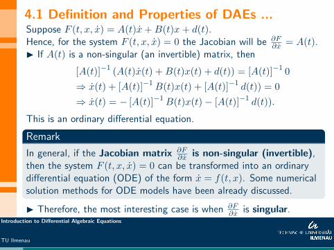
4.1 Definition and Properties of DAEs ...Suppose F (t, x, x) = A(t)x+B(t)x+ d(t).Hence, for the system F (t, x, x) = 0 the Jacobian will be ∂F

∂x = A(t).I If A(t) is a non-singular (an invertible) matrix, then

[A(t)]−1 (A(t)x(t) +B(t)x(t) + d(t)) = [A(t)]−1 0

⇒ x(t) + [A(t)]−1B(t)x(t) + [A(t)]−1 d(t)) = 0

⇒ x(t) = − [A(t)]−1B(t)x(t)− [A(t)]−1 d(t)).

This is an ordinary differential equation.

Remark

In general, if the Jacobian matrix ∂F∂x is non-singular (invertible),

then the system F (t, x, x) = 0 can be transformed into an ordinarydifferential equation (ODE) of the form x = f(t, x). Some numericalsolution methods for ODE models have been already discussed.

I Therefore, the most interesting case is when ∂F∂x is singular.


TU Ilmenau

4.2. Some DAE models from engineeringapplications

• There are several engineering applications that lead DAE modelequations.Examples: process engineering, mechanical engineering andmechatronics ( multibody Systems eg. robot dynamics, car dynamics,etc), electrical engineering (eg. electrical network systems, etc), waterdistribution network systems, thermodynamic systems, etc.

Frequently, DAEs arise from practical applications as:I differential equations describing the dynamics of the process, plusI algebraic equations describing:• laws of conservation of energy, mass, charge, current, etc.• mass, molar, entropy balance equations, etc.• desired constraints on the dynamics of the process.


TU Ilmenau

4.2. Some DAE models from engineeringapplications ... CSTRAn isothermal CSTR

A B → C.

Model equation:

V = Fa − F (5)

CA =Fa

V(CA0 − CA)−R1 (6)

CB = −Fa

VCB +R1 −R2 (7)

CC = −Fa

VCC +R2 (8)

0 = CA −CB

Keq(9)

0 = R2 − k2CB (10)


TU Ilmenau

4.2. Some DAE models from practical applications...a CSTR...• Fa-feed flow rate of A• CA0-feed concentration of A• R1, R2 - rates of reactions• F - product withdrawal rate• CA, CB, CC - concentration of species A, B and C, resp., in themixture.Definining

x = (V,CA, CB, CC)>

z = (R1, R2)>

the CSTR model equation can be written in the form

x = f(x, z)

0 = g(x, z).


TU Ilmenau

Some DAE models from practical applications...asimple pendulum

Newton’s Law:mx = −F

l xmy = mgF

l yConservation of mechanicalenergy: x2 + y2 = l2

(DAE) x1 = x3

x2 = x4

x3 = − F

m lx1

x4 = gF

lx2

0 = x2 + y2 − l2.Introduction to Differential Algebraic Equations

TU Ilmenau

Some DAE models from practical applications...anRLC circuit

Kirchhoff’s voltage and current lawsyield:

conservation of current:

iE = iR, iR = iC , iC = iL

conservation of energy:

VR + VL + VC + VE = 0

Ohm’s Laws:

CVC = iC , LVL = iL, VR = RiR


TU Ilmenau

Some DAE models from practical applications...anRLC circuit...

After replacing iR with iE and iC with iL we get a reducedDAE:

VC =1

CiL (11)

VL =1

LiL (12)

0 = VR +RiE (13)

0 = VE + VR + VC + VL (14)

0 = iL − iE (15)

(16)

Define x(t) = (VC , VL, VR, iL, iE)


TU Ilmenau

Some DAE models from practical applications...anRLC circuit...The RLC system can be written as:

x =

1C 0 0 0 00 1

L 0 0 00 0 0 0 00 0 0 0 00 0 0 0 0

x (17)

0 =

0 0 1 0 R1 1 1 0 00 0 0 1 −1

x+

010

VE (18)

which is of the form

x = Ax (19)

0 = Bx+Dz. (20)


TU Ilmenau

4.3. Classification of DAEs• Frequently, DAEs posses mathematical structure that are specific toa given application area.• As a result we have non-linear DAEs, linear DAEs, etc.• In fact, a knowledge on the mathematical structure of a DAEfacilitates the selection of model-specific algorithms and appropriatesoftware.Nonlinear DAEs:In the DAE F (t, x, x) = 0 if the function F is nonlinear w.r.t. any oneof t, x or x, then it is said to be a nonlinear DAE.

Linear DAEs: A DAE of the form

A(t)x(t) +B(t)x(t) = c(t),

where A(t) and B(t) are n× n matrices, is linear. If A(t) ≡ A andB(t) ≡ B, then we have time-invariant linear DAE.


TU Ilmenau

4.3. Classification of DAEs...Semi-explicit DAEs:A DAE given in the form

x = f(t, x, z) (21)

0 = g(t, x, z) (22)

• Note that the derivative of the variable z doesn’t appear in the DAE.• Such a variable z is called an algebraic variable; while x is called adifferential variable.• The equation 0 = g(t, x, z) called algebraic equation or aconstraint.

Examples:• The DAE model given for the RLC circuit, the CSTR and the simplependulum are all semi-explicit form.


TU Ilmenau

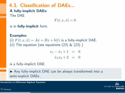
4.3. Classification of DAEs...A fully-implicit DAEs:The DAE

F (t, x, x) = 0

is in fully-implicit form.

Examples:(i) F (t, x, x) = Ax+Bx+ b(t) is a fully-implicit DAE.(ii) The equation (see equations (23) & (23) )

x1 − x1 + 1 = 0

x1x2 + 2 = 0

is a fully-implicit DAE.

I Any fully-implicit DAE can be always transformed into asemi-explicit DAEs .


TU Ilmenau

4.3. Classification of DAEs...Example (transformation of a fully-implicit DAE into a semi-explicitDAE):• Consider the linear time-invariant DAE Ax+Bx+ b(t) = 0 , whereλA+B is nonsingular, for some scalar λ. Then there are non-singularn× n matrices G and H such that:

GAH =

[Im OO N

]and GBH =

[J OO In−m

](23)

where Im the m×m identity matrix (here m ≤ n), N is an(n−m)× (n−m) nilpotent matrix; i.e., there is a positive integerp such that Np = 0, J ∈ Rm×m and In−m is the (n−m)× (n−m)identity matrix.I Now, we can write Ax+Bx+ b(t) = 0 equivalently as

(GAH) (H−1)x+ (GBH) (H−1)x+Gb(t) = 0. (24)


TU Ilmenau

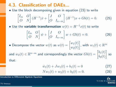
4.3. Classification of DAEs...• Use the block decomposing given in equation (23) to write[

Im OO N

](H−1)x+

[J OO In−m

](H−1)x+Gb(t) = 0. (25)

• Use the variable transformation w(t) = H−1x(t) to write[Im OO N

]w +

[J OO In−m

]w +Gb(t) = 0. (26)

• Decompose the vector w(t) as w(t) =

[w1(t)w2(t)

], with w1(t) ∈ Rm

and w2(t) ∈ Rn−m and correspondingly the vector Gb(t) =

[b1(t)b2(t)

]so

that:

w1(t) + Jw1(t) + b1(t) = 0 (27)

Nw1(t) + w2(t) + b2(t) = 0. (28)


TU Ilmenau

4.3. Classification of DAEs...

• Use now the nilpotent property of the matrix N ; i.e., multiply thesecond set of equation by Np−1 to get

w1(t) + Jw1(t) + b1(t) = 0 (29)

Npw1(t) +Np−1w2(t) +Np−1b2(t) = 0. (30)

From this it follows that (since Npw1(t) = 0)

w1(t) = −Jw1(t)− b1(t) (31)

0 = −Np−1w2(t)−Np−1b2(t). (32)

Therefore, we have transformed the fully-implicit DAEAx+Bx+ b(t) = 0 into a semi-explicit form.• Similarly, using mathematician manipulations, any nonlinearfully-implicit DAE can be transformed into a semi-explicit DAE.


TU Ilmenau

4.4. Index of a DAE• DAEs are usually very complex and hard to be solved analytically.⇒ DAEs are commonly solved by using numerical methods.

Question:Is it possible to use numerical methods of ODEs for the solution ofDAEs?

Idea:

Attempt to transform the DAE into an ODE.

• This can be chieved through repeated derivations of the algebraicequations g(t, x, z) = 0 with respect to time t.

Definition

The minimum number of differentiation steps required to transform aDAE into an ODE is known as the (differential) index of the DAE.


TU Ilmenau

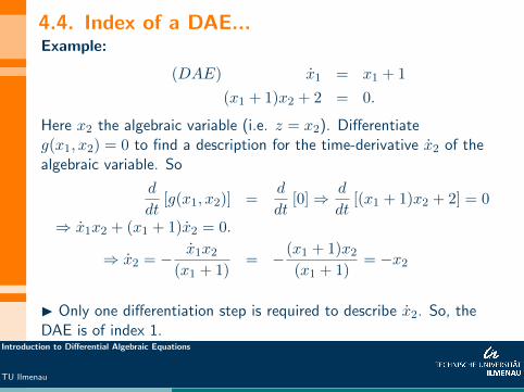
4.4. Index of a DAE...Example:

(DAE) x1 = x1 + 1

(x1 + 1)x2 + 2 = 0.

Here x2 the algebraic variable (i.e. z = x2). Differentiateg(x1, x2) = 0 to find a description for the time-derivative x2 of thealgebraic variable. So

d

dt[g(x1, x2)] =

d

dt[0]⇒ d

dt[(x1 + 1)x2 + 2] = 0

⇒ x1x2 + (x1 + 1)x2 = 0.

⇒ x2 = − x1x2(x1 + 1)

= −(x1 + 1)x2(x1 + 1)

= −x2

I Only one differentiation step is required to describe x2. So, theDAE is of index 1.


TU Ilmenau

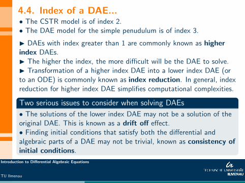
4.4. Index of a DAE...• The CSTR model is of index 2.• The DAE model for the simple penudulum is of index 3.

I DAEs with index greater than 1 are commonly known as higherindex DAEs.I The higher the index, the more difficult will be the DAE to solve.I Transformation of a higher index DAE into a lower index DAE (orto an ODE) is commonly known as index reduction. In general, indexreduction for higher index DAE simplifies computational complexities.

Two serious issues to consider when solving DAEs

• The solutions of the lower index DAE may not be a solution of theoriginal DAE. This is known as a drift off effect.• Finding initial conditions that satisfy both the differential andalgebraic parts of a DAE may not be trivial, known as consistency ofinitial conditions.


TU Ilmenau

4.4. Index of a DAE...Therefore, computational algorithms for a DAE should:

be cable of identifying consistent initial conditions to the DAE;as well as,provide automatic index reduction mechanisms to simplify theDAE.

I Modern software like Sundials, Modelica, use strategies forindex-reduction coupled with methods of consistent initialization.In the following we consider only index 1 semi-explicit DAEs:

(DAE) x = f(t, x, z) (33)

0 = g(t, x, z). (34)

Since ∂g∂t + ∂g

∂xdxdt + ∂g

∂zdzdt = 0. Hence, a semi-explicit DAE is of

index 1 iff[∂g∂z

]−1exists. That is, one differentiation step yields the

differential equation: dzdt = −

[∂g∂z

]−1 [∂g∂x

](f(t, x, z))−

[∂g∂z

]−1∂g∂t .


TU Ilmenau

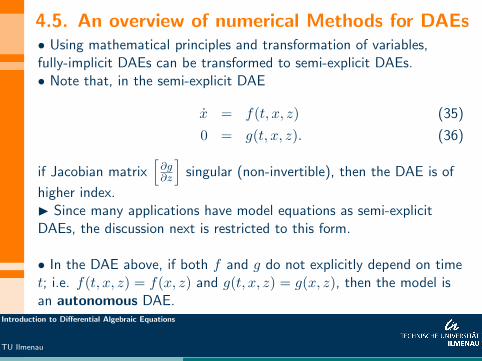
4.5. An overview of numerical Methods for DAEs• Using mathematical principles and transformation of variables,fully-implicit DAEs can be transformed to semi-explicit DAEs.• Note that, in the semi-explicit DAE

x = f(t, x, z) (35)

0 = g(t, x, z). (36)

if Jacobian matrix[∂g∂z

]singular (non-invertible), then the DAE is of

higher index.I Since many applications have model equations as semi-explicitDAEs, the discussion next is restricted to this form.

• In the DAE above, if both f and g do not explicitly depend on timet; i.e. f(t, x, z) = f(x, z) and g(t, x, z) = g(x, z), then the model isan autonomous DAE.


TU Ilmenau

4.5. An overview of numerical Methods for DAEs...I BDF and collocation methods are two most widely used methodsfor numerical solution of DAEs.

(I) BDF for DAEs:Consider the initial value DAE

x = f(t, x, z), x(t0) = x0 (37)

0 = g(t, x, z). (38)

Ideas of BDF:I Select a time step h so that ti+1 = ti + h, i = 0, 1, 2, . . .I Given xi = x(ti) and zi = z(ti), determine the valuexi+1 = x(ti+1) by using (extrapolating) values xi, xi−1, . . . , xi−m+1

of the current and earlier time instants of x(t).I Simultaneously compute zi+1 = z(ti+1).


TU Ilmenau

4.5. An overview of numerical Methods forDAEs...BDF• There is a unique m-th degree polynomial P that interpolates them+ 1 points

(ti+1, xi+1), (ti, xi), (ti−1, xi−1), . . . , (ti+1−m, xi+1−m).

• This interpolating polynomials P can be written as

P (t) =

m∑j=0

xi+1−jLj(t)

with the Lagrange polynomial

Lj(t) =

m∏l = 0l 6= j

[t− ti+1−l

ti+1−j − ti+1−l

], j = 0, 1, . . . ,m.


TU Ilmenau

4.5. ....BDF for DAEs...• Observe that

P (ti+1−j) = xi+1−j , j = 0, 1, . . . ,m.

In particular P (ti+1) = xi+1.• Thus, replace xi+1 by P (ti+1) to obtain

P (ti+1) = f(ti+1, xi+1). (∗)

But

P (ti+1) =

m∑j=0

xi+1−jLj(ti+1) = xi+1L0(ti+1) +

m∑j=1

xi+1−jLj(t)

Putting this into (*) we get:

xi+1 = −m∑j=1

xi+1−jLj(ti+1)

L0(ti+1)+

1

L0(ti+1)f(ti+1, xi+1)


TU Ilmenau

4.5. ....BDF for DAEs...Define

aj =Lj(ti+1)

L0(ti+1), bm =

1

hL0(ti+1).

• The values aj , j = 1, . . . ,m and bm can be read from lookup tables.

An m-step BDF Algorithm (BDF m) for a DAE:

Given a1, . . . , am,bm

xi+1 = −m∑j=1

ajxi+1−j + bmhf(ti+1, xi+1, zi+1) (39)

0 = g(ti+1, xi+1, zi+1). (40)

• Each iteration of the BDF requires a Newton algorithm for thesolution a system of nonlinear equations. Hence, the Jacobian ∂g

∂wneeds to be well-conditioned, where w = (t, x, z).


TU Ilmenau

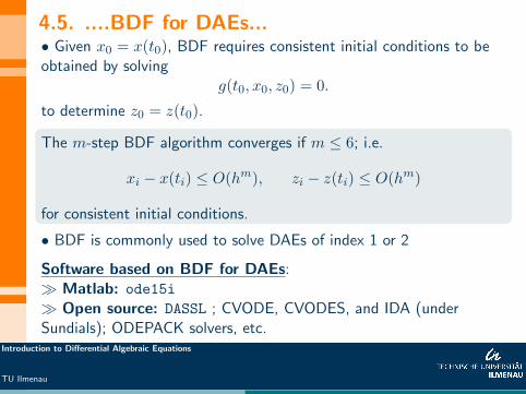
4.5. ....BDF for DAEs...• Given x0 = x(t0), BDF requires consistent initial conditions to beobtained by solving

g(t0, x0, z0) = 0.

to determine z0 = z(t0).

The m-step BDF algorithm converges if m ≤ 6; i.e.

xi − x(ti) ≤ O(hm), zi − z(ti) ≤ O(hm)

for consistent initial conditions.

• BDF is commonly used to solve DAEs of index 1 or 2

Software based on BDF for DAEs:� Matlab: ode15i

� Open source: DASSL ; CVODE, CVODES, and IDA (underSundials); ODEPACK solvers, etc.


TU Ilmenau


TU Ilmenau

Orthogonal Collocation• To collocate a function x(t) through another function p(t) = tocaptur the properties of x(t) by using p(t).• In general, we use a simpler function p(t) to collocate x(t); eg., p(t)can be a polynomial, a trigonometric function, etc.⇒ polynomial and trigonometric functions are usually simpler to workwith. (The discussion here is restricted to polynomilas)

Weirstraß’ Theorem

If x(t) is a continuous function on [a, b], then for any given ε > 0,there is a polynomial p(t) such that

maxa≤t≤b

|x(t)− p(t)| < ε

• Hence, we use the polynomial p(t) instead of x(t).• However, Weirstraß’ theorem doese not specifye how to constructthe approximating polynomial p(t) .


TU Ilmenau

• Suppose p(t) = a0 + a1t+ . . .+ amtm is the approximating

polynomial to x(t) on [a, b].Note: If the coefficients a0, a1, . . . , am are given, then theapproximating polynomial is exactly known.Question: How to determine a0, a1, . . . , am?Question: How to construct the apprximating polynomial?• There are several ways to construct p(t) to approximates x(t)according to Weirstraß’ theorem.Here we require p(t) to satisfy the following property:• p(ti) = x(ti) =: xi, i = 1, . . . , N.for some selected time instants t1, t2, . . . , tN from the interval [a, b].• This property relates p(t) and x(t) and is known as interpolatoryproperty.

Uniqueness of an interpolating polynamial

There is a unique interpolatory polynomial p(t) for the N data points(t1, x1),(t2, x2), . . .,(tN , xN ) with degree deg(p) = m = N − 1.


TU Ilmenau

• In the following we use N = m+ 1.Figure


TU Ilmenau

According to the interpolatory property, we have

x1 = p(t1) = a0 + a1t1 + . . .+ amtm1 (41)

x2 = p(t2) = a0 + a1t2 + . . .+ amtm2 (42)

... (43)

xm+1 = p(tm+1) = a0 + a1tm+1 + . . .+ amtmm+1. (44)

⇒

x1x2...

xm+1

=

1 t1 t21 . . . tm11 t2 t22 . . . tm2...

...... . . .

...1 tm+1 t2m+1 . . . tmm+1

a0a1...am

Thus, if we known x1, x2, . . . , xm+1 then we can computea0, a1, . . . , am and vice-versa.• But, since x(t) is not yet known, x1, x2, . . . , xm+1 are unknown.


TU Ilmenau

Hence, both

x1x2...

xm+1

and

a0a1...am

are unkowns.

• To avoid working with two unknown vectors, we can define thepolynamial p(t) in a better way as:

p(t) =

m+1∑i=1

xiLi(t) (45)

where Li(t) are Lagrange polynomials given by

Li(t) =

m+1∏j = 1j 6= i

t− tjti − tj

=(t− t1) (t− t2) . . . (t− ti−1) (t− ti+1) . . . (t− tm+1)

(ti − t1) (ti − t2) . . . (ti − ti−1) (ti − ti+1) . . . (ti − tm+1).


TU Ilmenau

Properties:

Li(tj) =

1, if i = j0, if i 6= j

? (satisfaction of the interpolatory property)

p(ti) = xi, i = 1, 2, . . . ,m+ 1.

? (approximation of x(t) by p(t))The polynomial p(t) in equation (45) can be made to satisfy theWeirstraß’ theorem by taking sufficiently large number of timeinstants t1, t2, . . . , tm+1 from [a, b].

Question: What is the best choice for t1, t2, . . . , tm+1?


TU Ilmenau

Determination of collocation Points

An idea to determine collocation points:

Select values τ1, τ2, . . . , τN from the interval [0, 1] and define the ti’sas follows:

ti = a+ τi(b− a), i = 1, . . . , N.

• This is a good idea, since the same values τ1, τ2, . . . , τN from [0, 1]can be used to generate collocation points on various intervals [a, b].Example:(i) If [a, b] = [2, 10], then ti = 2 + τi (10− 2) , i = 1, . . . , N ;(ii) If [a, b] = [0, 50], then ti = 0 + τi (50− 0) , i = 1, . . . , N ; etc.

Question: What is the best way to select the valuesτ1, τ2, . . . , τN from [0, 1]?


TU Ilmenau

Determination of collocation Points...

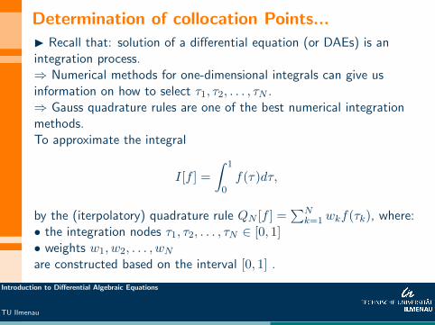
I Recall that: solution of a differential equation (or DAEs) is anintegration process.⇒ Numerical methods for one-dimensional integrals can give usinformation on how to select τ1, τ2, . . . , τN .⇒ Gauss quadrature rules are one of the best numerical integrationmethods.To approximate the integral

I[f ] =

∫ 1

0f(τ)dτ,

by the (iterpolatory) quadrature rule QN [f ] =∑N

k=1wkf(τk), where:• the integration nodes τ1, τ2, . . . , τN ∈ [0, 1]• weights w1, w2, . . . , wN

are constructed based on the interval [0, 1] .


TU Ilmenau

Determination of collocation points...Thus we would like to obtain the approximation

I[f ] =

∫ 1

0f(τ)dτ ≈ QN [f ] =

N∑i=1

wif(τi).

• Once a quadrature rule QN [·] is constructed it can be used toapproximate integrals of various functions.

Question: How to determine the 2N unknowns τ1, τ2, . . . , τN ,w1, w2, . . . , wN?

We require the quadrature rule to satisfy the equality:∫ b

aW (τ)p(τ)dτ =

N∑i=1

wip(τi)

for all polynomials p with degree deg(p) ≤ 2N .


TU Ilmenau

That is, QN [·] should integrate each of the polynomials

p(t) = 1, τ, τ2, . . . , τ2N

exactly. This implies ∫ 1

01dτ =

∑i=1

wi (46)∫ 1

0τdτ =

∑i=1

wiτi (47)∫ 1

0τ2dτ =

∑i=1

wiτ2i (48)

... (49)∫ 1

0τ2Ndτ =

∑i=1

wiτ2Ni . (50)


TU Ilmenau

We need to solve the system of 2N nonlinear equations:

1 = w1 + w2 + . . .+ wN (51)1

2= w1τ1 + w2τ2 + . . .+ wNτN (52)

(53)1

3= w1τ

21 + w2τ

22 + . . .+ wNτ

2N (54)

... (55)1

2N= w1τ

2N1 + w2τ

2N2 + . . .+ wNτ

2NN . (56)

From the equation 1 = w1 + w2 + . . .+ wN we can solve for w1 andreplace for it in the remaining equations.⇒ It remains to determine the 2N − 1 unknowns τ2, . . . , τN andw1, w2, . . . , wN from the reduced set of 2N − 1 equations.• Unfortunately, this system of equations is difficult to solve.


TU Ilmenau

Orthogonal polynomials

•There is a simpler way if we use orthogonal polynomials.I The concept of orthogonality requires a definition of scalarproduct.• The scalar product of functions h and g with respect on theinterval [0, 1] is

〈h, g〉 =

∫ 1

0h(τ)g(τ)dτ.

• Two functions h and g are orthogonal on the interval [0, 1] if

〈h, g〉 =

∫ 1

0h(τ)g(τ)dτ = 0.

• In this lecture, we are only interested in set of polynomials thatare orthogonal to each other.


TU Ilmenau

Orthogonal polynomials...• Orthogonal polynomials on [0, 1] (as defined above) are known asshifted Legendre polynomials.

Theorem (Three-term recurrence relation)

Suppose {p0, p1, . . .} the set of shifted Legendre orthogonalpolynomials on [0, 1] with deg(pn) = n and leading coefficient equalto 1. The shifted Legendre polynomials are generated by the relation

pn+1(τ) = (τ − an)pn(τ)− bnpn−1(τ)

with p0(τ) = 1 and p−1(τ) = 0, where the recurrence coefficients aregiven as

an = 12 , n = 0, 1, 2, . . .

bn = n2

4(4n2−1) , n = 0, 1, 2, . . .


TU Ilmenau

Orthogonal polynomials...The first four shifted Legendre orthogonal polynomials arep0(τ) = 1, p1(τ) = 2τ − 1, p2(τ) = 6τ2 − 6τ + 1, p3(τ) =20τ3 − 30τ2 + 12τ − 1.

Further important properties of orthogonal polynomials:Given any set of orthogonal polynomials {p0, p1, p2, . . .} the followinghold true:• Any finite set of orthogonal polynomials {p0, p1, . . . , pN−1} islinearly independent.• The polynomial PN is orthogonal to each of p0, p1, . . . , pN−1 .• Any non-zero polynomial q with degree deg(q) ≤ N − 1 can bewritten as a linear combination:

q(τ) = c0p0(τ) + c1p1(τ) + . . . , cN−1pN−1(τ)

where at least one of the scalars c0, c1, . . . , cN−1 is non-zero.Introduction to Differential Algebraic Equations

TU Ilmenau

Orthogonal polynomials...• We demand the quadrature rule is exact for polynomials up todegree 2N − 1.• Let P (τ) be any polynomial of degree 2N − 1.Hence,

I[P ] = QN [P ]⇒∫ 1

0P (τ)dτ =

N∑i=1

wiP (τi).

• Given the N -th degree orthogonal polynomial pN , the polynomial Pcan be written as

P (τ) = pN (τ)q(τ) + r(τ)

where q(τ) and r(τ) are polynomials such that 0 < deg(r) ≤ N − 1and• deg(q) = N − 1, since

2N − 1 = deg(P ) = deg(pN ) + deg(q) = N + deg(q).


TU Ilmenau

Orthogonal polynomials...• Now, from the equation

∫ 10 P (τ)dτ =

∑Nk=1wkP (τk) it follows that∫ b

a(pN (τ)q(τ) + r(τ)) dτ =

N∑i=1

wi (pN (τi)q(τk) + r(τi)) .

⇒∫ b

apN (τ)q(τ)dτ︸︷︷︸

=0

+��

��∫ b

ar(τ)dτ =

N∑i=1

wipN (τi)q(τi) +

��

��

��N∑i=1

wir(τi).

Observe the following:• Using polynomial exactness:

∫ ba r(τ)dτ =

∑Ni=1wi r(τi).

• Orthogonality implies < pN , pk >= 0, k = 1, . . . , N − 1. Thus,∫ ba pN (τ)q(τ) =∫ b

apN (τ)

N−1∑i=1

ckpk(τ)dτ =N−1∑k=1

ck

∫ b

apN (τ)pk(τ)dτ︸︷︷︸

=0

= 0.


TU Ilmenau

Orthogonal polynomials...It follows that

∑Nk=1wkpN (τk)q(τk) = 0. (?)

Theorem

If the quadrature nodes τ1, τ2, . . . , τN are zeros of the N−th degreeshifted Legendre polynomial pN (τ), then• all the roots τ1, τ2, . . . , τN lie inside (0, 1);• the quadrature weights are determined from

wi =

∫ 1

0Li(τ)dτ,

where Li(τ), i = 1, . . . , N is the Lagrange function defined usingτ1, τ2, . . . , τN and wi > 0, i = 1, . . . , N .• The quadrature rule QN [·] integrates polynomials degree up to2N − 1 exactly.

Hence, equation (?) holds true if p1(τ1) = pN (τ2) = . . . , p(τN ) = 0.Introduction to Differential Algebraic Equations

TU Ilmenau

Orthogonal polynomials...

• Therefore, the quadrature nodes τ1, τ2, . . . , τN are chosen as thezeros of the N -th degree shifted Legendre orthogonal polynomial.

Question:

Is there a simple way to compute the zeros τ1, τ2, . . . , τN of anorthogonal polynomial pN and the quadrature weightsw1, w2, . . . , wN?

The answer is give by a Theorem of Welsch & Glub (see next slide).


TU Ilmenau

Orthogonal polynomials...

Theorem (Welsch & Glub 1969 )

The quadrature nodes τ1, τ2, . . . , τN and weights w1, w2, . . . , wN canbe computed from the spectral factorization of

JN = V >ΛV ; Λ = diag(λ1, λ2, . . . , λN ), V V > = IN ;

of the symmetric tri-diagonal Jacobi matrix

JN =

a0√b1√

b1 a1√b2

√b2

. . .. . .

. . . aN−2√

bN−1√bN−1 aN−1

where

a0, an, bn, n = 1, . . . , N − 1 are the known coefficients from therecurrence relation. In particular ...


TU Ilmenau

Theorem ...

τk = λk, k = 1, . . . , N ; (57)

wk =(e>V ek

)2, k = 1, . . . , N, (58)

where e1, ek are the 1st and the k−the unit vectors of length N .

A Matlab program:

n = 5; format short

beta = .5./sqrt(1-(2*(1:n-1)).^(-2)); % recurr. coeffs

J = diag(beta,1) + diag(beta,-1) % Jacobi matrix

[V,D] = eig(J); % Spectral decomp.

tau = diag(D); [tau,i] = sort(tau); % Quad. nodes

w = 2*V(1,i).^2; % Quad. weights


TU Ilmenau

• There are standardised lookup tables for the integration nodesτ1, τ2, . . . , τN and corresponding weights w1, w2, . . . , wN .

The collocation points t1, t2, . . . , tN ∈ [a, b] can be determined byusing the quadrature points τ1, τ2, . . . , τN ∈ [0, 1] through therelation:

ti = a+ τi(b− a).

Example: Suppose we would like to collocate x(t) on [a, b] = [0, 10]using a polynomial x(t) with deg(x) = m = 3.• Required number of collocation points = N = m+ 1 = 3 + 1 = 4.⇒ First, determine the zeros of the 4-th degree shifted Legendrepolynomial p4(τ); i.e., find τ1, τ2, τ3, τ4 .• These value can be determined to be:

τ1 = 0.0694318442, τ2 = 0.3300094783,τ3 = 0.6699905218, τ4 = 0.9305681558.


TU Ilmenau

• Next, determine the collocation points :t1 = 0 + (10− 0) ∗ τ1 = 0.694318442, t2 = 0 + (10− 0) ∗ τ2 =

3.300094783,t3 = 0 + (10− 0) ∗ τ3 = 6.699905218,t4 = 0 + (10− 0) ∗ τ4 = 9.305681558.


TU Ilmenau

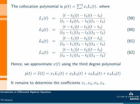
The collocation polynomial is p(t) =∑4

i xiLi(t). where

L1(t) =(t− t2)(t− t3)(t− t4)

(t1 − t2)(t1 − t3)(t1 − t4)(59)

L2(t) =(t− t1)(t− t3)(t− t4)

(t2 − t1)(t2 − t3)(t2 − t4)(60)

L3(t) =(t− t1)(t− t2)(t− t4)

(t3 − t1)(t3 − t2)(t3 − t4)(61)

L4(t) =(t− t1)(t− t2)(t− t3)

(t4 − t1)(t4 − t2)(t4 − t3). (62)

Hence, we approximate x(t) using the third degree polynomial

p(t) = x(t) = x1L1(t) + x2L2(t) + x3L3(t) + x4L4(t)

It remains to determine the coefficients x1, x2, x3, x4.


TU Ilmenau

Discretization of DAEs using orthogonal collocationsGiven the DAE:

x = f(t, x, z), t0 ≤ t ≤ tf (63)

0 = g(t, x, z) (64)

where x(t)> = (x1(t), x2(t), . . . , xn(t)) andz(t)> = (z1(t), z2(t), . . . , zm(t)).• Determine the a set of collocation points t1, t2, . . ., tN .• corresponding to each differential and algebraic variable definecollocation polynomials:

xk(t) −→ p(k)(t) =

N∑i=1

x(k)i Li(t), k = 1, . . . , n; (65)

zj(t) −→ p(j)(t) =

N∑i=1

z(j)i Li(t), j = 1, . . . ,m. (66)


TU Ilmenau

... orthogonal collocation of DAEs• In the DAE, replace xk(t) and zj(t) by q(k)(t) and p(j)(t) so that

p(1)(t) = f1(t,(p(1)(t), p(2)(t), . . . , p(n)(t)

),(q(1)(t), q(2)(t), . . . , q(m)(t)

))(67)

p(2)(t) = f2(t,(p(1)(t), p(2)(t), . . . , p(n)(t)

),(q(1)(t), q(2)(t), . . . , q(m)(t)

))(68)

... (69)

p(n)(t) = f1(t,(p(1)(t), p(2)(t), . . . , p(n)(t)

),(q(1)(t), q(2)(t), . . . , q(m)(t)

))(70)

0 = g1(t,(p(1)(t), p(2)(t), . . . , p(n)(t)

),(q(1)(t), q(2)(t), . . . , q(m)(t)

))(71)

0 = g2(t,(p(1)(t), p(2)(t), . . . , p(n)(t)

),(q(1)(t), q(2)(t), . . . , q(m)(t)

))(72)

... (73)

0 = gm(t,(p(1)(t), p(2)(t), . . . , p(n)(t)

),(q(1)(t), q(2)(t), . . . , q(m)(t)

))(74)


TU Ilmenau

... orthogonal collocation of DAEs• Next discretize the system above using t1, t2, . . . , tN to obtain:

p(1)(ti) = f1

(ti,(x(1)i , x

(2)i , . . . , x

(n)i

),(z(1)i , z

(2)i , . . . , z

(m)i

))p(2)(ti) = f2

(ti,(x(1)i , x

(2)i , . . . , x

(n)i

),(z(1)i , z

(2)i , . . . , z

(m)i

))...

p(n)(ti) = fn

(ti,(x(1)i , x

(2)i , . . . , x

(n)i

),(z(1)i , z

(2)i , . . . , z

(m)i

))0 = g1

(ti,(x(1)i , x

(2)i , . . . , x

(n)i

),(z(1)i , z

(2)i , . . . , z

(m)i

))0 = g2

(ti,(x(1)i , x

(2)i , . . . , x

(n)i

),(z(1)i , z

(2)i , . . . , z

(m)i

))...

0 = gm

(ti,(x(1)i , x

(2)i , . . . , x

(n)i

),(z(1)i , z

(2)i , . . . , z

(m)i

)),

i = 1, 2, . . . , N.Introduction to Differential Algebraic Equations

TU Ilmenau

... orthogonal collocation of DAEs• Solve the system of (n+m)×N equations to determine the

(n+m)×N unknwons x(k)i , k = 1, . . . , n, i = 1, . . . , N and

z(j)i , j = 1, . . . ,m, i = 1, . . . , N .

Example: Use a four point orthogonal collocation to solve the DAE

x1 = x1 + 1, 0 ≤ t ≤ 1.

0 = (x1 + 1)x2 + 2.

Solution: we use the collocation polynomials

p(1)(t) =

4∑i=1

x(1)i (t)Li(t) and p(2)(t) =

4∑i=1

x(2)i (t)Li(t)

to collocate x1(t) and x2(t), respectively.Introduction to Differential Algebraic Equations

TU Ilmenau

Advantages and disadvantages collocation methods

• can be used for higher index DAEs.• efficient for both initial value as well as boundary values DAEs.• more accurate

Disadvantages:• Can be computationally expensive• The approximating polynomials may display oscillatory properties,impacting accuracy• computational expenses become high if t1, t2, . . . , tN−1 areconsidered variables.


TU Ilmenau

Resources - LiteratureReferences:• U. M. Ascher, L. R. Petzold : Computer Methods for OrdinaryDifferential Equations and Differential-Algebraic Equations. SIAM1998.• K. E. Brenan, S. L. Campbell, and L.R. Petzold: (1996). NumericalSolution of Initial-Value Problems in Differential-Algebraic Equations.,SIAM, 1996.• Campbell, S. and Griepentrog, E., Solvability of General DifferentialAlgebraic Equations, SIAM J. Sci. Comput. 16(2) pp. 257-270, 1995.• M. S. Erik and G. Sderlind: Index Reduction inDifferential-Algebraic Equations Using Dummy Derivatives. SIAMJournal on Scientific Computing, vol. 14, pp. 677-692, 1993.• C. W. Gear : Differential-algebraic index transformation. SIAM J.Sci. Stat. Comp. Vol. 9, pp. 39 – 47, 1988.• Walter Gautschi: Orthogonal polynomials (in Matlab). Journal ofComputational and Applied Mathematics 178 (2005) 215– 234• Lloyd N. Trefethen: Is Gauss Quadrature Better thanClenshaw.Curtis? SIAM REVIEW, Vol. 50, No. 1, pp. 67 – 87, 2008.


TU Ilmenau

Resources - Literature .. Software• Pantelides Costas. (1988) ”The consistent initialization ofdifferential algebraic systems.” SIAM Journal on Scientific andStatistical Computing, vol. 9: 2, pp. 213–231, 1988.• L. Petzold: Differential/Algebraic Equations Are Not ODEs, SIAMJ. Sci. Stat. Comput. 3(3) pp. 367-384, 1982.Open source software:• DASSL - - FORTRAN 77:http://www.cs.ucsb.edu/ cse/software.html• DASSL Matlab interface:http://www.mathworks.com/matlabcentral/fileexchange/16917-dassl-mex-file-compilation-to-matlab-5-3-and-6-5• Sundials - https://computation.llnl.gov/casc/sundials/main.html• Modelica - https://modelica.org/• Odepack - http://www.cs.berkeley.edu/ kdatta/classes/lsode.html• Scicos- http://www.scicos.org/


TU Ilmenau

introduction to differential algebraic equations · pdf fileintroduction to di erential...

Documents