introduction to differential topology - peoplesalamon/preprints/difftop.pdf · differential...
TRANSCRIPT

INTRODUCTION TO
DIFFERENTIAL TOPOLOGY
Joel W. RobbinUW Madison
Dietmar A. SalamonETH Zurich
18 June 2018

ii

Preface
These are notes for the lecture course “Differential Geometry II” held by thesecond author at ETH Zurich in the spring semester of 2018. A prerequisiteis the foundational chapter about smooth manifolds in [21] as well as somebasic results about geodesics and the exponential map. For the benefit ofthe reader we summarize some of the relevant background material in thefirst chapter. The lecture course covered the content of Chapters 1 to 7(except Section 6.5).
The first half of this book deals with degree theory and the Pointare–Hopftheorem, the Pontryagin construction, intersection theory, and Lefschetznumbers. In this part we follow closely the beautiful exposition of Milnorin [14]. For the additional material on intersection theory and Lefschetznumbers a useful reference is the book by Guillemin and Pollack [9].
The second half of this book is devoted to differential forms and de Rhamcohomology. It begins with an elemtary introduction into the subject andcontinues with some deeper results such as Poincare duality, the Cech–deRham complex, and the Thom isomorphism theorem. Many of our proofsin this part are taken from the classical textbook of Bott and Tu [2] whichis also a highly recommended reference for a deeper study of the subject(including sheaf theory, homotopy theory, and characteristic classes).
18 June 2018 Joel W. Robbin and Dietmar A. Salamon
iii

iv

Contents
Introduction 1
1 Degree Theory Modulo Two 3
1.1 Smooth Manifolds and Smooth Maps . . . . . . . . . . . . . . 4
1.2 The Theorem of Sard and Brown . . . . . . . . . . . . . . . . 14
1.3 Proof of Sard’s Theorem . . . . . . . . . . . . . . . . . . . . . 23
1.4 The Degree Modulo Two of a Smooth Map . . . . . . . . . . 23
1.5 The Borsuk–Ulam Theorem . . . . . . . . . . . . . . . . . . . 23
2 The Brouwer Degree 25
2.1 Oriented Manifolds and the Brouwer Degree . . . . . . . . . . 25
2.2 Zeros of a Vector Field . . . . . . . . . . . . . . . . . . . . . . 25
2.2.1 Isolated Zeros . . . . . . . . . . . . . . . . . . . . . . . 25
2.2.2 Nondegenerate Zeros . . . . . . . . . . . . . . . . . . . 26
2.3 The Poincare–Hopf Theorem . . . . . . . . . . . . . . . . . . 27
3 Homotopy and Framed Cobordisms 29
3.1 The Pontryagin Construction . . . . . . . . . . . . . . . . . . 29
3.2 The Product Neighborhood Theorem . . . . . . . . . . . . . . 29
3.3 The Hopf Degree Theorem . . . . . . . . . . . . . . . . . . . . 29
4 Intersection Theory 31
4.1 Transversality . . . . . . . . . . . . . . . . . . . . . . . . . . . 31
4.2 Intersection Numbers . . . . . . . . . . . . . . . . . . . . . . . 40
4.2.1 Intersection Numbers Modulo Two . . . . . . . . . . . 40
4.2.2 Orientation and Intersection Numbers . . . . . . . . . 44
4.2.3 Isolated Intersections . . . . . . . . . . . . . . . . . . . 49
4.3 Self-Intersection Numbers . . . . . . . . . . . . . . . . . . . . 52
4.4 The Lefschetz Number of a Smooth Map . . . . . . . . . . . . 63
v

vi CONTENTS
5 Differential Forms 77
5.1 Exterior Algebra . . . . . . . . . . . . . . . . . . . . . . . . . 77
5.1.1 Alternating Forms . . . . . . . . . . . . . . . . . . . . 77
5.1.2 Exterior Product and Pullback . . . . . . . . . . . . . 80
5.1.3 Differential Forms on Manifolds . . . . . . . . . . . . . 83
5.2 The Exterior Differential and Integration . . . . . . . . . . . 86
5.2.1 The Exterior Differential on Euclidean Space . . . . . 86
5.2.2 The Exterior Differential on Manifolds . . . . . . . . . 90
5.2.3 Integration . . . . . . . . . . . . . . . . . . . . . . . . 92
5.2.4 The Theorem of Stokes . . . . . . . . . . . . . . . . . 94
5.3 The Lie Derivative . . . . . . . . . . . . . . . . . . . . . . . . 97
5.3.1 Cartan’s Formula . . . . . . . . . . . . . . . . . . . . . 97
5.3.2 Integration and Exactness . . . . . . . . . . . . . . . . 102
5.4 Volume Forms . . . . . . . . . . . . . . . . . . . . . . . . . . . 105
5.4.1 Integration and Degree . . . . . . . . . . . . . . . . . . 105
5.4.2 The Gauß–Bonnet Formula . . . . . . . . . . . . . . . 107
5.4.3 Moser Isotopy . . . . . . . . . . . . . . . . . . . . . . . 109
6 De Rham Cohomology 113
6.1 The Poincare Lemma . . . . . . . . . . . . . . . . . . . . . . . 114
6.2 The Mayer–Vietoris Sequence . . . . . . . . . . . . . . . . . . 120
6.2.1 Long Exact Sequences . . . . . . . . . . . . . . . . . . 120
6.2.2 Finite Good Covers . . . . . . . . . . . . . . . . . . . 125
6.2.3 The Kunneth Formula . . . . . . . . . . . . . . . . . . 127
6.3 Compactly Supported Differential Forms . . . . . . . . . . . . 130
6.3.1 Definition and Basic Properties . . . . . . . . . . . . . 130
6.3.2 The Mayer–Vietoris Sequence for H∗c . . . . . . . . . . 134
6.4 Poincare Duality . . . . . . . . . . . . . . . . . . . . . . . . . 139
6.4.1 The Poincare Pairing . . . . . . . . . . . . . . . . . . . 139
6.4.2 Proof of Poincare Duality . . . . . . . . . . . . . . . . 142
6.4.3 Poincare Duality and Intersection Numbers . . . . . . 144
6.4.4 Euler Characteristic and Betti Numbers . . . . . . . . 145
6.4.5 Examples and Exercises . . . . . . . . . . . . . . . . . 151
6.5 The Cech–de Rham Complex . . . . . . . . . . . . . . . . . . 155
6.5.1 The Cech Complex . . . . . . . . . . . . . . . . . . . . 155
6.5.2 The Isomorphism . . . . . . . . . . . . . . . . . . . . . 158
6.5.3 The Cech–de Rham Complex . . . . . . . . . . . . . . 160
6.5.4 Product Structures . . . . . . . . . . . . . . . . . . . . 166
6.5.5 Remarks on De Rham’s Theorem . . . . . . . . . . . . 168

CONTENTS vii
7 Vector Bundles and the Euler Class 171
7.1 Vector Bundles . . . . . . . . . . . . . . . . . . . . . . . . . . 171
7.2 The Thom Class . . . . . . . . . . . . . . . . . . . . . . . . . 179
7.2.1 Integration over the Fiber . . . . . . . . . . . . . . . . 179
7.2.2 The Thom Isomorphism Theorem . . . . . . . . . . . 183
7.2.3 Intersection Theory Revisited . . . . . . . . . . . . . . 189
7.3 The Euler Class . . . . . . . . . . . . . . . . . . . . . . . . . . 194
7.3.1 The Euler Number . . . . . . . . . . . . . . . . . . . . 194
7.3.2 The Euler Class . . . . . . . . . . . . . . . . . . . . . 198
7.3.3 The Product Structure on H∗(CPn) . . . . . . . . . . 203
8 Connections and Curvature 207
8.1 Connections . . . . . . . . . . . . . . . . . . . . . . . . . . . . 207
8.1.1 Vector Valued Differential Forms . . . . . . . . . . . . 207
8.1.2 Connections . . . . . . . . . . . . . . . . . . . . . . . . 208
8.1.3 Parallel Transport . . . . . . . . . . . . . . . . . . . . 213
8.1.4 Structure Groups . . . . . . . . . . . . . . . . . . . . . 214
8.1.5 Pullback Connections . . . . . . . . . . . . . . . . . . 218
8.2 Curvature . . . . . . . . . . . . . . . . . . . . . . . . . . . . . 219
8.2.1 Definition and basic properties . . . . . . . . . . . . . 219
8.2.2 The Bianchi Identity . . . . . . . . . . . . . . . . . . . 221
8.2.3 Gauge Transformations . . . . . . . . . . . . . . . . . 222
8.2.4 Flat Connections . . . . . . . . . . . . . . . . . . . . . 224
8.3 Chern–Weil Theory . . . . . . . . . . . . . . . . . . . . . . . . 228
8.3.1 Invariant Polynomials . . . . . . . . . . . . . . . . . . 228
8.3.2 Characteristic Classes . . . . . . . . . . . . . . . . . . 229
8.3.3 The Euler Class of an Oriented Rank-2 Bundle . . . . 232
8.3.4 Two Examples . . . . . . . . . . . . . . . . . . . . . . 236
8.4 Chern Classes . . . . . . . . . . . . . . . . . . . . . . . . . . . 239
8.4.1 Definition and Properties . . . . . . . . . . . . . . . . 239
8.4.2 Construction of the Chern Classes . . . . . . . . . . . 240
8.4.3 Proof of Existence and Uniqueness . . . . . . . . . . . 241
8.4.4 Tensor Products of Complex Line Bundles . . . . . . . 246
8.5 Chern Classes in Geometry . . . . . . . . . . . . . . . . . . . 248
8.5.1 Complex Manifolds . . . . . . . . . . . . . . . . . . . . 248
8.5.2 The Adjunction Formula . . . . . . . . . . . . . . . . . 250
8.5.3 Complex Surfaces . . . . . . . . . . . . . . . . . . . . 252
8.5.4 Almost Complex Structures on Four-Manifolds . . . . 259
8.6 Low-Dimensional Manifolds . . . . . . . . . . . . . . . . . . . 260

viii CONTENTS
A Notes 265A.1 Paracompactness . . . . . . . . . . . . . . . . . . . . . . . . . 265A.2 Partitions of Unity . . . . . . . . . . . . . . . . . . . . . . . . 268A.3 Embedding a Manifold into Euclidean Space . . . . . . . . . . 272A.4 The Exponential Map . . . . . . . . . . . . . . . . . . . . . . 278A.5 Classifying Smooth One-Manifolds . . . . . . . . . . . . . . . 279
References 281
Index 282

Introduction
1

2 CONTENTS

Chapter 1
Degree Theory Modulo Two
In this and the following two chapters we follow closely the beautiful book“Topology from the Differentiable Viewpoint” by Milnor [14]. Milnor’s mas-terpiece of mathematical exposition cannot be improved. The only excusewe can offer for including the material in this book is for completeness ofthe exposition. There are, nevertheless, two minor points in which the firstthree chapters of this book differ from [14]. The first is that our expositionuses the intrinsic notion of a smooth manifold. The basic definitions areincluded in Section 1.1 and the proofs of some foundational theorems suchas the existence of partitions of unity and of embeddings in Euclidean spaceare relegated to the appendix. For a more extensive discussion of these con-cepts the reader is referred to the two introductory chapters of [21] whichare understood as prerequisites for the present book. A second minor pointof departure from Milnor’s text is the inclusion of the Borsuk–Ulam theoremin Section 1.5 at the end of the present chapter. The other four section ofthis chapter correspond to the first four chapters of Milnor’s book. Afterthe introductory section, which includes a proof of the fundamental theo-rem of algebra, we discuss Sard’s theorem, manifolds with boundary, andthe Brouwer Fixed Point Theorem in Section 1.2, include a proof of Sard’sTheorem in Section 1.3, and introduce the degree modulo two of a smoothmap in Section 1.4. Throughout we assume that the reader is familiar withfirst year analysis and the basic notions of point set topology.
3

4 CHAPTER 1. DEGREE THEORY MODULO TWO
1.1 Smooth Manifolds and Smooth Maps
Let U ⊂ Rm and V ⊂ Rn be open sets. A map f : U → V is called smoothiff it is infinitely differentiable, i.e. iff all its partial derivatives
∂αf =∂α1+···+αmf
∂xα11 · · · ∂x
αmm, α = (α1, . . . , αm) ∈ Nm0 ,
exist and are continuous. For a smooth map f = (f1, . . . , fn) : U → V anda point x ∈ U the derivative of f at x is the linear map df(x) : Rm → Rndefined by
df(x)ξ :=d
dt
∣∣∣∣t=0
f(x+ tξ) = limt→0
f(x+ tξ)− f(x)
t, ξ ∈ Rm.
This linear map is represented by the Jacobian matrix of f at x whichwill also be denoted by
df(x) :=
∂f1∂x1
(x) · · · ∂f1∂xm
(x)...
...∂fn∂x1
(x) · · · ∂fn∂xm
(x)
∈ Rn×m.
Note that we use the same notation for the Jacobian matrix and the cor-responding linear map from Rm to Rn. The derivative satisfies the chainrule. Namely, if U ⊂ Rm, V ⊂ Rn, W ⊂ Rp are open sets and f : U → Vand g : V →W are smooth maps then g f : U →W is smooth and
d(g f)(x) = dg(f(x)) df(x) : Rm → Rp (1.1.1)
for every x ∈ U . Moreover the identity map idU : U → U is always smoothand its derivative at every point is the identity map of Rm. This impliesthat, if f : U → V is a diffeomorphism (i.e. f is bijective and f and f−1
are both smooth), then its derivative at every point is an invertible linearmap and so m = n. The Inverse Function Theorem (see below) is a kind ofconverse.
Following Milnor [14], we extend the definition of smooth map to mapsbetween subsets X ⊂ Rm and Y ⊂ Rn which are not necessarily open. Inthis case a map f : X → Y is called smooth if for each x0 ∈ X there existsan open neighborhood U ⊂ Rm of x0 and a smooth map F : U → Rn thatagrees with f on U ∩X. A map f : X → Y is called a diffeomorphismif f is bijective and f and f−1 are smooth. When there exists a diffeomor-phism f : X → Y then X and Y are called diffeomorphic. When X and Yare open these definitions coincide with the usage above.

1.1. SMOOTH MANIFOLDS AND SMOOTH MAPS 5
Smooth Manifolds
Definition 1.1.1 (Smooth m-Manifold). Let m ∈ N0. A smooth m-manifold is a topological space M , equipped with an open cover Uαα∈Aand a collection of homeomorphisms φα : Uα → Ωα onto open sets Ωα ⊂ Rm(see Figure 1.1) such that, for each pair α, β ∈ A, the transition map
φβα := φβ φ−1α : |φα(Uα ∩ Uβ)→ φβ(Uα ∩ Uβ) (1.1.2)
is smooth. The homeomorphisms φα are called coordinate charts and thecollection A := Uα, φαα∈A is called an atlas.
M
Uα βU
βαφβφα φ
Figure 1.1: Coordinate charts and transition maps.
Let (M,A = Uα, φαα∈A) be a smooth m-manifold. Then a sub-set U ⊂M is open if and only if φα(U ∩ Uα) is an open subset of Rm forevery α ∈ A. Thus the topology on M is uniquely determined by the at-las. A homeomorphism φ : U → Ω from an open set U ⊂M to an openset Ω ⊂ Rm is called compatible with the atlas A if the transitionmap φα φ−1 : φ(U ∩ Uα)→ φα(U ∩ Uα) is a diffeomorphism for each α.The atlas A is called maximal if it contains every coordinate chart thatis compatible with all its members. Thus every atlas A is contained ina unique maximal atlas A , consisting of all coordinate charts φ : U → Ωthat are compatible with A . Such a maximal atlas is also called a smoothstructure on the topological space M . We do not distinguish the mani-folds (M,A ) and (M,A ′) if the corresponding maximal atlasses agree, i.e. ifthe charts of A ′ are all compatible with A (and vice versa) or, equivalently,if the union A ∪A ′ is again a smooth atlas. If this holds, we say that Aand A ′ induce the same smooth structure on M .
Example 1.1.2. The m-sphere Sm :=x ∈ Rm+1 |x2
1 + · · ·+ x2m+1 = 1
is
a smooth manifold with the atlas φ± : U± → Rm given by
U± := Sn \ (0, . . . , 0,∓1), φ±(x) :=
(x1
1± xm+1, . . . ,
xn1± xm+1
).

6 CHAPTER 1. DEGREE THEORY MODULO TWO
Example 1.1.3. The real m-torus is the topological space
Tm := Rm/Zm
equipped with the quotient topology. Thus two vectors x, y ∈ Rm are equiv-alent if their difference x − y ∈ Zm is an integer vector and we denoteby π : Rm → Tm the obvious projection which assigns to each vector x ∈ Rmits equivalence class
π(x) := [x] := x+ Zm.
Then a set U ⊂ Tm is open if and only if the set π−1(U) is an open subsetof Rm. An atlas on Tm is given by the open cover
Uα := [x] |x ∈ Rm, |x− α| < 1/2 ,
parametrized by vectors α ∈ Rm, and the coordinate charts φα : Uα → Rmdefined by φα([x]) := x for x ∈ Rm with |x− α| < 1/2. Exercise: Showthat each transition map for this atlas is a translation by an integer vector.
Example 1.1.4. The complex projective space CPn is the set
CPn =` ⊂ Cn+1 | ` is a 1-dimensional complex subspace
of complex lines in Cn+1. It can be identified with the quotient
CPn =(Cn+1 \ 0
)/C∗
of the space of nonzero vectors in Cn+1 modulo the action of the multiplica-tive group C∗ = C \0 of nonzero complex numbers. The equivalence classof a nonzero vector z = (z0, . . . , zn) ∈ Cn+1 will be denoted by
[z] = [z0 : z1 : · · · : zn] := λz |λ ∈ C∗
and the associated line is ` = Cz. An atlas on CPn is given by the opencover Ui := [z0 : · · · : zn] | zi 6= 0 for i = 0, 1, . . . , n and the coordinatecharts φi : Ui → Cn are
φi([z0 : · · · : zn]) :=
(z0
zi, . . . ,
zi−1
zi,zi+1
zi, . . . ,
znzi
). (1.1.3)
Exercise: Prove that each φi is a homeomorphism and the transition mapsare holomorphic. Prove that the manifold topology is the quotient topology,i.e. if π : Cn+1 \ 0 → CPn denotes the obvious projection, then a sub-set U ⊂ CPn is open if and only if π−1(U) is an open subset of Cn+1 \ 0.

1.1. SMOOTH MANIFOLDS AND SMOOTH MAPS 7
Example 1.1.5. The real projective space RPn is the set
RPn =` ⊂ Rn+1 | ` is a 1-dimensional linear subspace
of real lines in Rn+1. It can again be identified with the quotient
RPn =(Rn+1 \ 0
)/R∗
of the space of nonzero vectors in Rn+1 modulo the action of the multiplica-tive group R∗ = R \ 0 of nonzero real numbers, and the equivalence classof a nonzero vector x = (x0, . . . , xn) ∈ Rn+1 will be denoted by
[x] = [x0 : x1 : · · · : xn] := λx |λ ∈ R∗ .
An atlas on RPn is given by the open cover
Ui := [x0 : · · · : xn] |xi 6= 0
and the coordinate charts φi : Ui → Rn are again given by (1.1.3), with zjreplaced by xj . The arguments in Example 1.1.4 show that these coordinatecharts form an atlas and the manifold topology is the quotient topology. Thetransition maps are real analytic diffeomorphisms.
Example 1.1.6. Consider the complex Grassmannian
Gk(Cn) := V ⊂ Cn | v is a k-dimensional complex linear subspace .
This set can again be described as a quotient space Gk(Cn) ∼= Fk(Cn)/U(k).Here
Fk(Cn) :=D ∈ Cn×k |D∗D = 1l
denotes the set of unitary k-frames in Cn and the group U(k) acts on Fk(Cn)contravariantly by D 7→ Dg for g ∈ U(k). The projection
π : Fk(Cn)→ Gk(Cn)
sends a matrix D ∈ Fk(Cn) to its image V := π(D) := im D. A sub-set U ⊂ Gk(Cn) is open if and only if π−1(U) is an open subset of Fk(Cn).Every k-dimensional subspace V ⊂ Cn determines an open set UV ⊂ Gk(Cn)consisting of all k-dimensional subspaces of Cn that can be represented asgraphs of linear maps from V to V ⊥. This set of graphs can be identifiedwith the space HomC(V, V ⊥) of complex linear maps from V to V ⊥ andhence with C(n−k)×k. This leads to an atlas on Gk(Cn) with holomorphictransition maps and shows that Gk(Cn) is a manifold of complex dimen-sion k(n − k). Exercise: Verify the details of this construction. Findexplicit formulas for the coordinate charts and their transition maps. Carrythis over to the real setting. Show that CPn and RPn are special cases.

8 CHAPTER 1. DEGREE THEORY MODULO TWO
Example 1.1.7 (The real line with two zeros). A topological space Mis called Hausdorff if any two points in M can be separated by disjointopen neighborhoods. This example shows that a manifold need not be aHausdorff space. Consider the quotient space
M := R× 0, 1/ ≡
where [x, 0] ≡ [x, 1] for x 6= 0. An atlas on M consists of two coordinatecharts φ0 : U0 → R and φ1 : U1 → R where
Ui := [x, i] |x ∈ R , φi([x, i]) := x
for i = 0, 1. Thus M is a 1-manifold. But the topology on M is notHausdorff, because the points [0, 0] and [0, 1] cannot be separated by disjointopen neighborhoods.
Example 1.1.8 (A 2-manifold without a countable atlas). Considerthe vector space X = R× R2 with the equivalence relation
[t1, x1, y2] ≡ [t2, x2, y2] ⇐⇒ either y1 = y2 6= 0, t1 + x1y1 = t2 + x2y2
or y1 = y2 = 0, t1 = t2, x1 = x2.
For y 6= 0 we have [0, x, y] ≡ [t, x − t/y, y], however, each point (x, 0) onthe x-axis gets replaced by the uncountable set R× (x, 0). Our manifoldis the quotient space M := X/ ≡ with the topology induced by the atlasdefined below. (This is not the quotient topology.) The coordinate chartsare parametrized by the reals: for t ∈ R the set Ut ⊂M and the coordinatechart φt : Ut → R2 are given by
Ut := [t, x, y] |x, y ∈ R , φt([t, x, y]) := (x, y).
A subset U ⊂M is open, by definition, if φt(U ∩Ut) is an open subset of R2
for every t ∈ R. With this topology each φt is a homeomorphism from Utonto R2 and M admits a countable dense subset S := [0, x, y] |x, y ∈ Q.However, there is no atlas on M consisting of countably many charts. (Eachcoordinate chart can contain at most countably many of the points [t, 0, 0].)The function f : M → R given by f([t, x, y]) := t + xy is smooth and eachpoint [t, 0, 0] is a critical point of f with value t. Thus f has no regularvalue. Exercise: Show that M is a path-connected Hausdorff space.
Throughout this book we will tacitly assume that manifolds are Haus-dorff and second countable. This excludes pathological examples such asExample 1.1.7 and Example 1.1.8. Theorem A.3.1 shows that smooth man-ifolds whose topology is Hausdorff and second countable are precisely thosethat can be embedded in Euclidean space.

1.1. SMOOTH MANIFOLDS AND SMOOTH MAPS 9
Smooth Maps
Definition 1.1.9 (Smooth Map). Let
(M, (φα, Uα)α∈A), (N, (ψβ, Vβ)β∈B)
be smooth manifolds. A map f : M → N is called smooth if it is continuousand the map
fβα := ψβ f φ−1α : φα(Uα ∩ f−1(Vβ))→ ψβ(Vβ) (1.1.4)
is smooth for every α ∈ A and every β ∈ B. It is called a diffeomorphismif it is bijective and f and f−1 are smooth. The manifolds M and N arecalled diffeomorphic if there exists a diffeomorphism f : M → N .
The reader may verify that compositions of smooth maps are smooth,and that the identity map is smooth.
Example 1.1.10. The map T1 → S1 : [t] 7→ (cos(2πt), sin(2πt)) is a diffeo-morphism.
Example 1.1.11. The map f : S2 → CP1 defined by
f(x) :=
[1 + x3 : x1 + ix2], if x 6= (0, 0,−1),[0 : 1], if x = (0, 0,−1),
for x = (x1, x2, x3) ∈ S2 is a diffeomorphism whose inverse is given by
f−1([z0 : z1]) =
(2Re(z0z1)
|z0|2 + |z1|2,
2Im(z0z1)
|z0|2 + |z1|2,|z0|2 − |z1|2
|z0|2 + |z1|2
)for [z0 : z1] ∈ CP1.
Example 1.1.12. Let p(z) = a0 + a1z + a2z2 + · · ·+ adz
d be a polynomialwith complex coefficients. Then the map f : CP1 → CP1 defined by
f([z0 : z1]) :=[zd0 : a0z
d0 + a1z
d−10 z1 + · · ·+ ad−1z0z
d−11 + adz
d1
]for [z0 : z1] ∈ CP1 is smooth.
Example 1.1.13. Let A ∈ Zn×m and le b ∈ Rn. Then the map x 7→ Ax+ bdescends to a smooth map f : Tm → Tn.
Smooth manifolds and smooth maps between them form a categorywhose isomorphisms are diffeomorphisms. The subject of differential topol-ogy can roughly be described as the study of those properties of smoothmanifolds that are invariant under diffeomorphisms. A longstanding openproblem in the field is of whether every smooth four-manifold that is homeo-morphic to the four-sphere is actually diffeomorphic to the four-sphere. Thisis known as the four-dimensional smooth Poincare conjecture.
10 CHAPTER 1. DEGREE THEORY MODULO TWO
Tangent Spaces and Derivatives
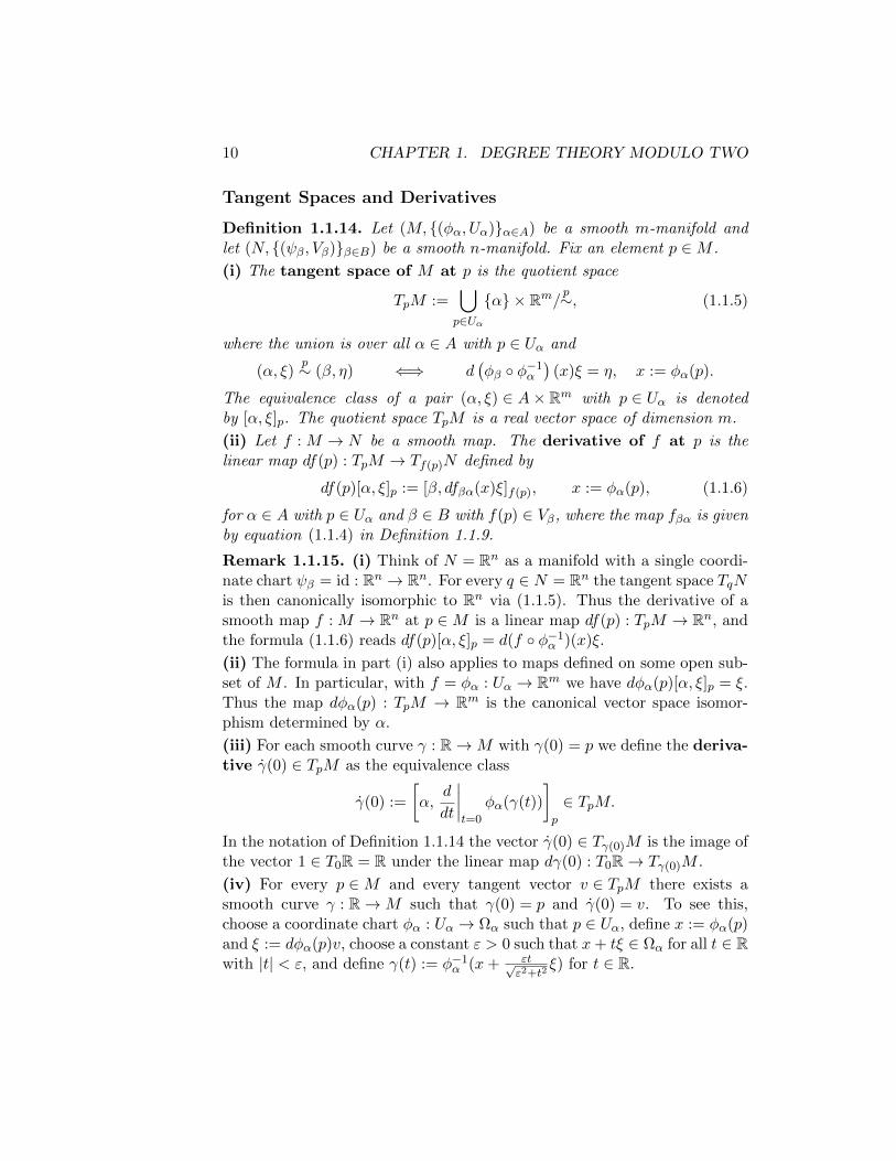
Definition 1.1.14. Let (M, (φα, Uα)α∈A) be a smooth m-manifold andlet (N, (ψβ, Vβ)β∈B) be a smooth n-manifold. Fix an element p ∈M .
(i) The tangent space of M at p is the quotient space
TpM :=⋃p∈Uα
α × Rm/ p∼, (1.1.5)
where the union is over all α ∈ A with p ∈ Uα and
(α, ξ)p∼ (β, η) ⇐⇒ d
(φβ φ−1
α
)(x)ξ = η, x := φα(p).
The equivalence class of a pair (α, ξ) ∈ A× Rm with p ∈ Uα is denotedby [α, ξ]p. The quotient space TpM is a real vector space of dimension m.
(ii) Let f : M → N be a smooth map. The derivative of f at p is thelinear map df(p) : TpM → Tf(p)N defined by
df(p)[α, ξ]p := [β, dfβα(x)ξ]f(p), x := φα(p), (1.1.6)
for α ∈ A with p ∈ Uα and β ∈ B with f(p) ∈ Vβ, where the map fβα is givenby equation (1.1.4) in Definition 1.1.9.
Remark 1.1.15. (i) Think of N = Rn as a manifold with a single coordi-nate chart ψβ = id : Rn → Rn. For every q ∈ N = Rn the tangent space TqNis then canonically isomorphic to Rn via (1.1.5). Thus the derivative of asmooth map f : M → Rn at p ∈M is a linear map df(p) : TpM → Rn, andthe formula (1.1.6) reads df(p)[α, ξ]p = d(f φ−1
α )(x)ξ.
(ii) The formula in part (i) also applies to maps defined on some open sub-set of M . In particular, with f = φα : Uα → Rm we have dφα(p)[α, ξ]p = ξ.Thus the map dφα(p) : TpM → Rm is the canonical vector space isomor-phism determined by α.
(iii) For each smooth curve γ : R→M with γ(0) = p we define the deriva-tive γ(0) ∈ TpM as the equivalence class
γ(0) :=
[α,
d
dt
∣∣∣∣t=0
φα(γ(t))
]p
∈ TpM.
In the notation of Definition 1.1.14 the vector γ(0) ∈ Tγ(0)M is the image ofthe vector 1 ∈ T0R = R under the linear map dγ(0) : T0R→ Tγ(0)M .
(iv) For every p ∈M and every tangent vector v ∈ TpM there exists asmooth curve γ : R→M such that γ(0) = p and γ(0) = v. To see this,choose a coordinate chart φα : Uα → Ωα such that p ∈ Uα, define x := φα(p)and ξ := dφα(p)v, choose a constant ε > 0 such that x+ tξ ∈ Ωα for all t ∈ Rwith |t| < ε, and define γ(t) := φ−1
α (x+ εt√ε2+t2
ξ) for t ∈ R.

1.1. SMOOTH MANIFOLDS AND SMOOTH MAPS 11
The Inverse Function Theorem
A fundamental property of the derivative is the chain rule. It asserts that,if f : M → N and g : N → P are smooth maps between smooth manifolds,then the derivative of the composition g f : M → P at p ∈M is given by
d(g f)(p) = dg(q) df(p), q := f(p) ∈ N.
In other words, to every commutative triangle
Ng
@@@
@@@@
@
M
f>>|||||||| gf // P
.
of smooth maps between smooth manifolds M,N,P and every p ∈M therecorresponds a commutative triangle of linear maps
TqNdg(q)
""EEE
EEEE
E
TpM
df(p)<<xxxxxxxx gf // TrP
,
where q := f(p) ∈ N and r := g(q) ∈ P . A second fundamental observa-tion is that the derivative of the identity map f = idM : M →M at eachpoint p ∈M is the identity map of the tangent space, i.e. didM (p) = idTpM .
Lemma 1.1.16. Let f : M → N be a diffeomorphism between smooth man-ifolds and let p ∈M . Then the derivative df(p) : TpM → Tf(p)N is a vectorspace isomorphism. In particular, M and N have the same dimension.
Proof. Let g := f−1 : N →M be the inverse map and let q := f(p) ∈ N .Then g f = idM and so dg(q) df(p) = d(g f)(p) = idTpM by the chainrule. Likewise df(p) dg(q) = idTqN and so df(p) is a vector space isomor-phism with inverse dg(q) : TqN → TpM .
A partial converse of Lemma 1.1.16 is the inverse function theorem.
Theorem 1.1.17 (Inverse Function Theorem). Let M and N be smoothm-manifolds and let f : M → N be a smooth map. Let p0 ∈M and supposethat the derivative df(p0) : Tp0M → Tf(p0)N is a vector space isomorphism.Then there exists an open neighborhood U ⊂M of p0 such that V := f(U)is an open subset of N and the restriction f |U : U → V is a diffeomorphism.
Proof. For maps between open subsets of Euclidean space a proof can befound in [22, Appendix C]. The general case follows by applying the specialcase to the map fβα in Definition 1.1.9.

12 CHAPTER 1. DEGREE THEORY MODULO TWO
Regular Values
Definition 1.1.18 (Regular value). Let M be a smooth m-manifold, let Nbe a smooth n-manifold, and let f : M → N be a smooth map. An ele-ment p ∈M is a called a regular point of f if df(p) : TpM → TqN issurjective and is called a critical point of f if df(p) is not surjective. Anelement q ∈ N is called a regular value of f if the set f−1(q) containsonly regular points and is called a critical value of f if it is not a regularvalue, i.e. if there exists an element p ∈M such that f(p) = q and df(p) isnot surjective. The set of critical points of f will be denoted by
Cf :=p ∈M
∣∣ df(p) : TpM → Tf(p)N is not surjective.
Thus f(Cf ) ⊂ N is the set of critical values of f and its complement
Rf := N \ f(Cf )
is the set of regular values of f .
Remark 1.1.19. Let f : M → N be as in Definition 1.1.18.
(i) The set Cf of critical points of f is a closed subset of M . If M iscompact, if follows that Cf is a compact subset of M , hence its image f(Cf )is a compact and therefore closed subset of N , and so the set Rf of regularvalues of f is open.
(ii) Assume M is compact and dim(M) = dim(N) and let q ∈ N be a reg-ular value of f . Then the set f−1(q) ⊂M is closed and therefore com-pact. Moreover, f−1(q) consists of isolated points. Namely, if p ∈ f−1(q)then df(p) : TpM → TqN is bijective, hence by the Inverse Function Theo-rem 1.1.17 there exists an open neighborhood U ⊂M of p such that f |U isinjective, and this implies U ∩ f−1(q) = p. Since f−1(q) is compact andconsists of isolated points, it is a finite subset of M .
(iii) Assume M is compact and dim(M) = dim(N). Then Rf ⊂ N is openby (i) and #f−1(q) <∞ for all q ∈ Rf by (ii). We prove that the map
Rf → N0 : q 7→ #f−1(q)
is locally constant. Fix a regular value q ∈ N of f , assume k := #f−1(q) > 0,and write f−1(q) = p1, . . . , pk. By the Inverse Function Theorem 1.1.17there exist open neighborhoods Ui ⊂M of pi and Vi ⊂ N of q such that f |Uiis a diffeomorphism from Ui to Vi for each i. Shrinking the Ui, if necessary,we may assume that Ui ∩ Uj = ∅ for i 6= j. Then the set
V := V1 ∩ · · · ∩ Vk \ f(M \ (U1 ∪ · · · ∪ Uk))
is open, satisfies q ∈ V ⊂ Rf , and #f−1(q′) = k for all q′ ∈ V .

1.1. SMOOTH MANIFOLDS AND SMOOTH MAPS 13
The Fundamental Theorem of Algebra
Let
p : C→ C
be a nonconstant polynomial. Thus there exists a positive integer d andcomplex numbers a0, a1, . . . , ad ∈ C such that
ad 6= 0
and
p(z) = a0 + a1z + a2z2 + · · ·+ adz
d
for all z ∈ C. Define the map f : CP1 → CP1 by
f([z0 : z1]) := [zd0 : a0zd0 + a1z
d−10 z1 + · · ·+ ad−1z0z
d−11 + adz
d1 ]
= [1 : p(z1/z0)]
for [z0 : z1] ∈ CP1, where the last equation holds in the case z0 6= 0 (seeExample 1.1.12). The set of critical points of f is given by
Cf =
[1 : z]
∣∣∣∣ z ∈ C, p′(z) =d∑
k=1
kakzk−1 = 0
∪
[0 : 1]
Thus Cf is a finite subset of CP1 and so the set
Rf = CP1 \ f(Cf )
of regular values of f is connected. Hence it follows from part (iii) of Re-mark 1.1.19 that the function
Rf → N : q 7→ #f−1(q)
is constant. Since f is not constant, we have #f−1(q) > 0 for all q ∈ Rf .Since CP1 is compact, an approximation argument shows that #f−1(q) > 0for all q ∈ CP1 and hence, in particular,
#f−1([1 : 0]) > 0.
Thus there exists a complex number z ∈ C such that p(z) = 0 and this provesthe fundamental theorem of algebra.
14 CHAPTER 1. DEGREE THEORY MODULO TWO
1.2 The Theorem of Sard and Brown
On page 13 we have seen that the set of singular values of a polynomialmap from CP1 to itself is finite. In general, the set of singular values of asmooth map may be infinite, however, it has Lebesgue measure zero in eachcoordinate chart. This is the content of Sard’s Theorem [23], proved in 1942after earlier work by A.P. Morse [18].
Theorem 1.2.1 (Sard). Let U ⊂ Rm be an open set, let f : U → Rn be asmooth map, and denote the set of critical points of f by
C := x ∈ U | the derivative df(x) : Rm → Rn is not surjective .
Then the set f(C) ⊂ Rn of critical values of f has Lebesgue measure zero.
Proof. See page 23.
Since a set of Lebesgue measure zero connot contain any nonempty openset, it follows from Theorem 1.2.1 that the set Rn \ f(C) of regular valuesof f is dense in Rn. This was proved by A.P. Brown [4, Thm 3-III] in 1935and rediscovered by Dubovitskii [7] in 1953 and by Thom [24] in 1954.
Theorem 1.2.1 is not sharp. It actually suffices to assume that f is aC`-map, where ` ≥ 1 + max0,m− n. The proof of this stronger versioncan be found in [1]. For the applications in this book it suffices to assumethat f is smooth as in Theorem 1.2.1. The proof in Section 1.3 is taken fromMilnor [14] and requires the existence of many derivatives.
Corollary 1.2.2 (Sard–Brown). Let M be a smooth m-manifold (whosetopology is second countable and Hausdorff), let N be a smooth n-manifold,let f : M → N be a smooth map, and let Cf ⊂M be the set of critical pointsof f (where the derivative df(p) : TpM → Tf(p)N is not surjective). Then theset f(Cf ) of critical values of f has Lebesgue measure zero in each coordinatechart and the set Rf := N \ f(Cf ) of regular values of f is dense in N .
Proof. Since M is paracompact by Lemma A.1.4, it admits a countableatlas Uα, φαα∈A. Let ψ : V → Ω ⊂ Rn be a coordinate chart on N and,for each α ∈ A, define the map fα := ψfφ−1
α : Ωα := φα(Uα∩f−1(V ))→ Ωand denote by Cα ⊂ Ωα the set of critical points of fα. By Theorem 1.2.1the set fα(Cα) ⊂ Rn has Lebesgue measure zero for every α ∈ A. Since A iscountable, the set ψ(f(Cf )∩V )) =
⋃α∈A fα(Cα) ⊂ Ω has Lebesgue measure
zero. Hence the set ψ(Rf ∩ V ) = Ω \ ψ(f(Cf ) ∩ V ) is dense in Ω. Since thisholds for each coordinate chart on N , it follows that Rf is dense in N . Thisproves Corollary 1.2.2.

1.2. THE THEOREM OF SARD AND BROWN 15
Submanifolds
Definition 1.2.3. Let M be a smooth m-manifold and let P ⊂M . Thesubset P is called a d-dimensional submanifold of M if, for every ele-ment p ∈ P , there exists an open neighborhood U ⊂M of p and a coordinatechart φ : U → Ω with values in an open set Ω ⊂ Rm such that
φ(U ∩ P ) = Ω ∩ (Rd × 0). (1.2.1)
Let P ⊂M be a d-dimensional submanifold of a smooth m-manifold M .Then P is a smooth d-manifold in its own right. The topology on P is therelative topology as a subset of M and the smooth structure is determinedby the coordinate charts ψ := π φ|U∩P → Rd, where φ : U → Ω ⊂ Rm is acoordinate chart on M that satisfies (1.2.1) and π : Rm → Rd denotes theprojection π(x1, . . . , xm) := (x1, . . . , xd). By part (iv) of Remark 1.1.15, thetangent space of P at p ∈ P can be naturally identified with the space
TpP =v ∈ TpM
∣∣∣ there exists a smooth curve γ : R→Msuch that γ(R) ⊂ P, γ(0) = p, γ(0) = v
.
Lemma 1.2.4. Let M be a smooth m-manifold, let N be a smooth n-manifold, let f : M → N be a smooth map, and let q ∈ N be a regular valueof f . Then the set P := f−1(q) is an (m−n)-dimensional submanifold of Mand its tangent space at p ∈ P is given by TpP = ker df(p).
Proof. Let d := m− n and let p0 ∈ P . Then df(p0) is surjective and thisimplies dim(ker df(p0)) = d. Choose a linear map Φ0 : Tp0M → Rd whoserestriction to ker df(p0) is bijective and, by Exercise 1.2.5, choose a smoothmap g : M → Rd such that g(p0) = 0 and dg(p0) = Φ0. Define the smoothmap F : M → Rd ×N by F (p) := (g(p), f(p)) for p ∈M . Then the deriva-tive dF (p0) = Φ0 × df(p0) : Tp0M → Rd × TqN is bijective. Hence the In-verse Function Theorem 1.1.17 asserts that there exists an open neigh-borhood U ⊂M of p0 such that F (U) ⊂ Rd ×N is an open neighborhoodof F (p0) = (0, q) and F |U : U → F (U) is a diffeomorphism. Shrinking U ifnecessary, we may assume that f(U) ⊂ V , where V ⊂ N is an open neigh-borhood of q which admits a coordinate chart ψ : V → Rn. Then the coor-dinate chart φ : U → Rm, defined by φ(p) := (g(p), ψ(f(p))) for p ∈ U , sat-isfies equation (1.2.1) in Definition 1.2.3. Moreover, if p ∈ P and v ∈ TpP ,then there exists a smooth curve γ : R→ P such that γ(0) = p and γ(0) = vhence df(p)v = d
dt
∣∣t=0
f(γ(t)) = 0, and so df(p)v = 0. Thus TpP ⊂ ker df(p)and, since both subspaces have dimension d, this proves Lemma 1.2.4.
Exercise 1.2.5. For every p ∈M and every linear map Λ : TpM → R thereexists a smooth function f : M → R such that f(p) = 0 and df(p) = Λ.

16 CHAPTER 1. DEGREE THEORY MODULO TWO
Manifolds with Boundary
This section introduces the concept of a manifold with boundary. Fix apositive integer m and introduce the notations
Hm :=x = (x1, . . . , xm) ∈ Rm
∣∣xm ≥ 0,
∂Hm :=x = (x1, . . . , xm) ∈ Rm
∣∣xm = 0,
(1.2.2)
for the m-dimensional upper half space and its boundary.
βαφβφα φ
αU Uβ
M
Figure 1.2: A manifold with boundary.
Definition 1.2.6. A smooth m-manifold with boundary consists of a(second countable Haudorff) topological space M , and open cover Uαα∈Aof M , and a collection of homeomorphisms
φα : Uα → Ωα
onto open subsets Ωα ⊂ Hm, one for every α ∈ A, such that, for everypair α, β ∈ A, the transition map
φβα := φβ φ−1α : φα(Uα ∩ Uβ)→ φβ(Uα ∩ Uβ)
is a diffeomorphism (see Figure 1.2). The homeomorphisms φα : Uα → Ωα
are called coordinate charts, the collection φα, Uαα∈A is called an atlasof M , and the subset
∂M =p ∈M
∣∣φα(p) ∈ ∂Hm for every α ∈ A with p ∈ Uα. (1.2.3)
is called the boundary of M .

1.2. THE THEOREM OF SARD AND BROWN 17
Remark 1.2.7. Let (M, φα, Uαα∈A) be a manifold with boundary.
(i) The domain Ωαβ := φα(Uα ∩ Uβ) ⊂ Hm of the transition map φβα inDefinition 1.2.6 need not be an open subset of Rm. If x ∈ Ωαβ ∩ ∂Hm is aboundary point of Ωαβ, then the map φβα is called smooth near x iff thereexists an open neighborhood U ⊂ Rm of x and a smooth map Φ : U → Rmsuch that Φ(x) = φβα(x) for all x ∈ Ωαβ ∩ U .
(ii) If p ∈M and let α, β ∈ A such that p ∈ Uα ∩ Uβ. Then
φα(p) ∈ ∂Hm ⇐⇒ φβ(p) ∈ ∂Hm (1.2.4)
To see this, assume that x := φα(p) ∈ Ωαβ \ ∂Hm and φβ(p) ∈ ∂Hm. Thenthe mth coordinate φβα,m : Ωαβ → R has a local minimum at x and hencethe Jacobi matrix dφβα(x) is not invertible, a contradiction.
(iii) The boundary ∂M admits the natural structure of an (m−1)-manifoldwithout boundary. (Exercise: Prove this.)
(iv) The tangent space of M at p ∈M is defined as the quotient
TpM :=⋃p∈Uα
α × Rm/∼ (1.2.5)
under the equivalence relation
(α, ξ) ∼ (β, η)def⇐⇒ η = dφβα(φα(p))ξ.
Thus the tangent space at each boundary point p ∈ ∂M is a vector space(and not a half space). For p ∈M and α ∈ A such that p ∈ Uα, define thelinear map
dφα(p) : TpM → Rm
by
dφα(p)v := ξ for v = [α, ξ] ∈ TpM.
Here [α, ξ] denotes the equivalence class of the pair (α, ξ) with ξ ∈ Rm.
(v) Let p ∈ ∂M . A tangent vector v ∈ TpM is called outward pointing if
dφα(p)v ∈ Rm \Hm
for some, and hence every, α ∈ A such that p ∈ Uα. (Exercise: Prove thatthis condition is independent of the choice of α.)

18 CHAPTER 1. DEGREE THEORY MODULO TWO
Lemma 1.2.8. Let M be a smooth m-manifold without boundary and sup-pose that g : M → R is a smooth function such that 0 is a regular value of g.Then the set
M0 :=p ∈M
∣∣ g(x) ≥ 0
is an m-manifold with boundary
∂M0 :=p ∈M
∣∣ g(x) = 0.
Proof. Fix an element p0 ∈M such that g(p0) = 0. By [21, Theorem 2.2.17]the set g−1(0) ⊂M is a smooth (m − 1)-dimensional submanifold of M .Hence there exists an open neighborhood U ⊂M of p0 and a coordinatechart φ : U → Ω with values in an open set Ω ⊂ Rm such that
φ(U ∩ g−1(0)) = Ω ∩ (Rm−1 × 0).
Adding a constant vector in Rm−1 ×0 to φ and shrinking U , if necessary,we may assume without loss of generality that
φ(p0) = 0, Ω =x ∈ Rm
∣∣ |x| < r
for some constant r > 0. Thus, for every p ∈ U , we have
g(p) = 0 ⇐⇒ φm(p) = 0.
Thus (g φ−1)(x) = 0 for all x ∈ Ω with xm = 0. Since zero is a regular valueof g, this implies that ∂
∂xm(g φ−1)(x) 6= 0 for all x = (x1, . . . , xm−1, 0) ∈ Ω.
This set is connected and so the sign is independent of x. Replacing φ byits composition with the reflection (x1, . . . , xm) 7→ (x1, . . . , xm−1,−xm), ifnecessary, we may assume that
∂
∂xm(g φ−1)(x) > 0 for all x = (x1, . . . , xm−1, 0) ∈ Ω.
Since Ω = x ∈ Rm | |x| < r, this implies
p ∈ U ∩M0 ⇐⇒ φm(p) ≥ 0
for all p ∈ U . Thus U0 := U ∩M0 = p ∈ U | g(p) ≥ 0 is an open neoghbor-hood of p0 with respect to the relative topology of M0 and
φ0 : U0 → Ω0 :=x ∈ Ω
∣∣xm ≥ 0⊂ Hm
is a homeomorphism. Cover M0 by such open sets to obtain an atlas withsmooth transition maps. This proves Lemma 1.2.8.

1.2. THE THEOREM OF SARD AND BROWN 19
Example 1.2.9. The closed unit disc
Dm := x ∈ Rm | |x| ≤ 1
is a smooth manifold with boundary ∂Dm = Sm−1 =x ∈ Rm
∣∣ |x| = 1
.This follows from Lemma 1.2.8 with M = Rm and g(x) = 1−
∑mi=1 x
2i .
In Lemma 1.2.8 the manifold M has empty boundary, the submani-fold M0 ⊂M has codimension zero. and near each boundary point of M0
there exists a coordinate chart of M on an open set U ⊂M that sends theintersection U ∩M0 to an open subset of the upper half space Hm. Thenext definition introduces the notion of a submanifold with boundary of anycodimension such that the boundary of the submanifold is contained in theboundary of the ambient manifold M .
φ
0
Rm−n
nR
Um
ΩX
H
x
F (0)−1
Figure 1.3: A submanifold with boundary.
Definition 1.2.10. Let M be a smooth m-manifold with boundary. A sub-set X ⊂M is called a d-dimensional submanifold with boundary
∂X = X ∩ ∂M,
if, for every p ∈ X, there exists an open neighborhood U ⊂M of p and acoordinate chart φ : U → Ω with values in an open set Ω ⊂ Hm such that
φ(U ∩X) = Ω ∩ (0 ×Hd). (1.2.6)
Exercise 1.2.11. Let M be a smooth m-manifold without boundary. Calla subset X ⊂M a d-dimensional submanifold with boundary if, for ev-ery p ∈ X, there exists an open neighborhood U ⊂M of p and a coordinatechart φ : U → Ω with values in an open set Ω ⊂ Rm that satisfies (1.2.6).Prove that the set M0 in Lemma 1.2.8 satisfies this definition with d = m.Prove that a closed subset M0 ⊂M is an m-dimensional submanifold withboundary if and only if its boundar ∂M0 = M0 \ int(M0) agrees with theboundary of its interior and is an (m− 1)-dimensional submanifold of M .

20 CHAPTER 1. DEGREE THEORY MODULO TWO
Lemma 1.2.12. Let M be a smooth m-manifold with boundary, let N be asmooth n-manifold without boundary, let f : M → N be a smooth map, andlet q ∈ N be a regular value of f and a regular value of f |∂M . Then the set
X := f−1(q) =p ∈M
∣∣ f(p) = q⊂M
is an (m− n)-dimensional submanifold with boundary ∂X = X ∩ ∂M .
Proof. This is a local statement. Hence it suffices to assume that M = Hm
and N = Rn and q = 0 ∈ Rn.Let f : Hm → Rn be a smooth map such that zero is a regular value
of f and of f |∂Hm . If f−1(0) ∩ ∂Hm = ∅ the result follows from [21, Theo-rem 2.2.17]. Thus assume f−1(0) ∩ ∂Hm 6= ∅ and let x ∈ ∂Hm with f(x) = 0.Choose an open neighborhood U ⊂ Rm of x and a smooth map F : U → Rnsuch that F (x) = f(x) for all x ∈ U ∩Hm. Since zero is a regular valueof f the derivative dF (x) = df(x) : Rm → Rn is surjective. Now denoteby e1, . . . , em the standard basis of Rm. We prove the following.
Claim. There exist integers 1 ≤ i1 < · · · < in ≤ m− 1 such that
spanei1 , . . . , ein ∩ ker dF (x) = 0 (1.2.7)
Denote by v1, . . . , vm ∈ Rn the columns of the Jacobi matrix dF (x) ∈ Rn×m.Then the linear map d(f |∂Hm)(x) : Tx∂Hm = Rm−1 × 0 → Rn is givenby d(f |∂Hm)(x)ξ =
∑m−1i=1 ξivi for ξ = (ξ1, . . . , ξm−1, 0) ∈ Rm−1 × 0. Since
this linear map is surjective, there exist integers 1 ≤ i1 < · · · < in ≤ m− 1such that det(vi1 , . . . , vin) 6= 0. These indices satisfy (1.2.7) and this provesthe claim. Reordering the coordinates x1, . . . , xm−1, if necessary, we mayassume without loss of generality that iν = ν for ν = 1, . . . , n.
Now define the map Φ : U → Rm = Rn × Rm−n by
Φ(x) := (F (x), xn+1, . . . , xm) for x = (x1, . . . , xm) ∈ U.
Then dΦ(x)ξ = (dF (x)ξ, ξn+1, . . . , ξm) for ξ = (ξ1, . . . , ξm) ∈ Rm. By theclaim with iν = ν for ν = 1, . . . , n the linear map dΦ(x) : Rm → Rm is in-jective and hence bijective. Thus the inverse function theorem asserts thatthe restriction of Φ to a sufficiently small neighborhood of x is a diffeomor-phism onto its image. Shrink U , if necessary, to obtain that Φ(U) is an opensubset of Rm and Φ : U → Φ(U) is a diffeomorphism. Then U ∩Hm is anopen neighborhood of x in M = Hm, the set Ω := Φ(U ∩Hm) = Φ(U) ∩Hm
is an open subset of Hm, the restriction φ := Φ|U∩Hm : U ∩Hm → Ω is adiffeomorphism and hence a coordinate chart of M , and
φ(U ∩X) = Ω ∩ (0 ×Hm−n)
(see Figure 1.3). This proves Lemma 1.2.12.

1.2. THE THEOREM OF SARD AND BROWN 21
The Brouwer Fixed Point Theorem
Recall from Example 1.2.9 that the closed unit disc
Dm :=x ∈ Rm |x2
1 + x22 + · · ·+ x2
m ≤ 1
in Rm is a smooth manifold with boundary ∂Dm = Sm−1. The followingfixed point theorem was proved by L.E.J. Brouwer [3] in 1910.
Theorem 1.2.13 (Brouwer Fixed Point Theorem). Every continuousmap g : Dm → Dm has a fixed point.
Proof. See page 22.
Brouwer’s Fixed Point Theorem extends to continuous maps from anynonempty compact convex subset of Rm to itself. An infinite-dimensionalvariant of this result is the Tychonoff Fixed Point Theorem [25] whichasserts that, if C is a nonempty compact convex subset of a locally convextopological vector space, then every continuous map g : C → C has a fixedpoint. Another generalization of Brouwer’s Fixed Point Theorem is theLefschetz Fixed Point Theorem in Corollary 4.4.4.
Following Milnor [14] we will first prove Theorem 1.2.13 for smooth mapand then use an approximation argument to establish the result for all con-tinuous maps. In the smooth case the proof is based on the following keylemma which uses Sard’s Theorem 1.2.1 about the existence of regular valuesand Lemma 1.2.12 about the preimages of regular values.
Lemma 1.2.14. Let M be a compact smooth manifold with boundary. Theredoes not exist a smooth map f : M → ∂M that restricts to the identity mapon the boundary.
Proof. Suppose that there exists a smooth map f : M → ∂M such that
f(p) = p for all p ∈ ∂M.
By Corollary 1.2.2 there exists a regular value q ∈ ∂M of f . Since q is alsoa regular value of the identity map id = f |∂M , it follows from Lemma 1.2.12that the set X := f−1(q) is a compact smooth 1-dimensional manifold witha single boundary point
∂X = f−1(q) ∩ ∂M = q.
However, Theorem A.5.1 asserts that X is a finite union of circles and arcsand hence must have an even number of boundary points. This contradictionproves Lemma 1.2.14.

22 CHAPTER 1. DEGREE THEORY MODULO TWO
Lemma 1.2.15. Let g : Dm → Dm be a smooth map. Then there exists anelement x ∈ Dm such that g(x) = x.
Proof. Suppose g(x) 6= x for every x ∈ Dm. For x ∈ Dm let f(x) ∈ Sm−1 bethe unique intersection point of the straight line through x and g(x) that iscloser to x than to g(x) (see Figure 1.4). Then f(x) = x for all x ∈ Sm−1.An explicit formula for f(x) is
f(x) = x+ tu, u :=x− g(x)
|x− g(x)|, t :=
√1− |x|2 + 〈x, u〉2 − 〈x, u〉.
This formula shows that the map f : Dm → Sm−1 is smooth. Such a mapdoes not exist by Lemma 1.2.14. Hence our assumption that g does not havea fixed point must have been wrong, and this proves Lemma 1.2.15.
f(x)
x
g(x)
Figure 1.4: Proof of Brouwer’s Fixed Point Theorem.
Proof of Theorem 1.2.13. Let g : Dm → Dm be a continuous map and as-sume that g(x) 6= x for all x ∈ Dm. Then, since Dm is a compact subsetof Rm, there exists a constant ε > 0 such that |g(x)− x| ≥ 2ε for all x ∈ Dm.By the Weierstraß Approximation Theorem (see for example [5, Thm 5.4.5]with M = Dm and A the set of polynomials in m variables with real coeffi-cients), there exists a polynomial map p : Dm → Rm such that
|p(x)− g(x)| < ε for all x ∈ Dm.
Define the map q : Dm → Rm by
q(x) :=p(x)
1 + εfor x ∈ Dm.
Then |q(x)| ≤ 1 and
|q(x)− g(x)| = |p(x)− g(x)− εg(x)|1 + ε
≤ |p(x)− g(x)|1 + ε
+ε|g(x)|1 + ε
< 2ε
for all x ∈ Dm. Thus q : Dm → Dm is a smooth map without fixed points,in contradiction to Lemma 1.2.15. This proves Theorem 1.2.13.

1.3. PROOF OF SARD’S THEOREM 23
1.3 Proof of Sard’s Theorem
Proof of Theorem 1.2.1.
1.4 The Degree Modulo Two of a Smooth Map
1.5 The Borsuk–Ulam Theorem

24 CHAPTER 1. DEGREE THEORY MODULO TWO

Chapter 2
The Brouwer Degree
2.1 Oriented Manifolds and the Brouwer Degree
2.2 Zeros of a Vector Field
2.2.1 Isolated Zeros
Let M be a smooth manifold without boundary and let X ∈ Vect(M).
Definition 2.2.1 (Isolated Zero). A point p0 ∈M is called an isolatedzero of X if X(p0) = 0 and there exists an open set U ⊂M such that p0 ∈ Uand X(p) 6= 0 for all p ∈ U \ p0.
The goal of this section is to assign an index ι(p0, X) ∈ Z to each isolatedzero of X. As a first step we consider the special case of a smooth vectorfield ξ : Ω→ Rm on an open set Ω ⊂ Rm.
Definition 2.2.2 (Index). Let Ω ⊂ Rm be an open set, let ξ : Ω→ Rm bea smooth vector field, and let x0 ∈ Ω be an isolated zero of ξ. Choose ε > 0such that, for all x ∈ Rm,
0 < |x| ≤ ε =⇒ ξ(x) 6= 0.
Then the integer
ι(x0, ξ) := deg
(Sm−1 → Sm−1 : x 7→ ξ(x0 + εx)
|ξ(x0 + εx)|
)(2.2.1)
is independent of the choice of ε and is called the index of ξ at x0.
25

26 CHAPTER 2. THE BROUWER DEGREE
2.2.2 Nondegenerate Zeros
Lemma 2.2.3. Let X ∈ Vect(M) and let p ∈M be a nondgenerate zeroof X. Then p is an isolated zero of X and
ι(p,X) = sign(det(DX(p))
)=
+1, if DX(p) is orientation preserving,−1, if DX(p) is orientation reversing.
(2.2.2)
Proof.

2.3. THE POINCARE–HOPF THEOREM 27
2.3 The Poincare–Hopf Theorem
Theorem 2.3.1 (Poinare–Hopf). Let M be a compact smooth m-dimen-sional manifold with boundary and let X ∈ Vect(M) be a smooth vector fieldon M that points out on the boundary. Assume that X has only isolatedzeros. Then ∑
p∈M,X(p)=0
ι(p,X) =
m∑k=0
(−1)k dim(Hk(M)), (2.3.1)
where H∗(M) denotes the de Rham cohomology of M . In particular, the lefthand side is independent of the choice of the vector field X. It is called theEuler characteristic of M and is denoted by
χ(M) :=∑
p∈M,X(p)=0
ι(p,X). (2.3.2)
Proof. See page 28.
Theorem 2.3.1 was proved in 1885 by Poincare in the case dim(M) = 2.After partial results by Brouwer and Hadamard, the theorem was establishedin full generality in 1926 by Hopf.
In this section we will only prove that the sum of the indices of the zerosof a vector field with with only isolated zeros that points out on the boundaryis independent of the choice of the vector field. The formula (2.3.1) for thede Rham cohomology groups will be established in Theorem 6.4.8.
Lemma 2.3.2 (Hopf). Let N ⊂ Rn be a compact smooth n-dimensionalsubmanifold with boundary, i.e. N is compact and its boundary agrees withthe boundary of its interior and is a smooth (n−1)-dimensional submanifoldof Rn. Let Y : N → Rn be a smooth vector field with only isolated zeros suchthat Y (x) 6= 0 for all x ∈ ∂N . Then∑
x∈N, Y (x)=0
ι(x, Y ) = deg
(Y
|Y |: ∂N → Sn−1
). (2.3.3)
If, in addition, the vector field Y points out of N on the boundary, then
deg
(Y
|Y |: ∂N → Sn−1
)= deg(g), (2.3.4)
where g : ∂N → Sn−1 denotes the Gauß map, i.e. for every x ∈ ∂N theunit vector g(x) ∈ Sn−1 is orthogonal to Tx∂N and points out of N , sothat x+ tg(x) ∈ Rn \N for every sufficiently small real number t > 0.
Proof.

28 CHAPTER 2. THE BROUWER DEGREE
Lemma 2.3.3. Let M be a smooth manifold with boundary, let X be asmooth vector field on M , and let p0 ∈M \ ∂M be an isolated zero of X.Choose an open neighborhood U ⊂M \ ∂M of p0 such that p0 is the onlyzero of X in U . Then there exists a smooth vector field X ′ on M suchthat X ′(p) = X(p) for all p ∈M \ U, the zeros of X ′ in U are all nondegen-erate, and ∑
p∈U,X′(p)=0
ι(p,X ′) = ι(p0, X). (2.3.5)
Proof.
Proof of Theorem 2.3.1.

Chapter 3
Homotopy and FramedCobordisms
The purpose of the present chapter is to extend the degree theory developedin Chapters 1 and 2 to smooth maps between manifolds of different dimen-sions, with the dimension of the source being bigger than the dimension ofthe target.
3.1 The Pontryagin Construction
3.2 The Product Neighborhood Theorem
3.3 The Hopf Degree Theorem
29

30 CHAPTER 3. HOMOTOPY AND FRAMED COBORDISMS

Chapter 4
Intersection Theory
The purpose of the present chapter is to extend the degree theory developedin Chapters 1 and 2 to smooth maps between manifolds of different dimen-sions, with the dimension of the source being smaller than the dimension ofthe target. The relevant transversality theory is the subject of Section 4.1,orientation and intersection numbers are introduced in Section 4.2, self-intersection numbers are discussed in Section 4.3, and Section 4.4 examinesthe Lefschetz number of a smooth map from a compact manifold to itselfand establishes the Lefschetz–Hopf theorem and the Lefschetz fixed pointtheorem.
4.1 Transversality
This section introduces the notion of transversality of a smooth map to asubmanifold of the target space.
Definition 4.1.1 (Transversality). Let m,n, k be nonnegative integerssuch that k ≤ n, let M be a smooth m-manifold, let N be a smooth n-manifold, and let Q ⊂ N be a smooth submanifold of dimension n− k. Thenumber k is called the codimension of Q and is denoted by
codim(Q) := dim(N)− dim(Q).
Let f : M → N be a smooth map and let p ∈ f−1(Q). The map f is said tobe transverse to Q at p if
Tf(p)N = im (df(p)) + Tf(p)Q (4.1.1)
It is called transverse to Q if it is transverse to Q at every p ∈ f−1(Q). Thenotation f −t Q signifies that the map f is transverse to the submanifold Q.
31

32 CHAPTER 4. INTERSECTION THEORY
f
QM
Figure 4.1: Transverse and nontransverse intersections.
Example 4.1.2. (i) If Q = N , then every smooth map f : M → N is trans-verse to Q.
(ii) If Q = q is a single point in N , then a smooth map f : M → N istransverse to Q if and only if q is a regular value of f .
(iii) If f : M → N is an embedding, then its image P := f(M) is a smoothsubmanifold of N (see [21, Theorem 2.3.4]). In this situation f is transverseto Q if and only if
TqN = TqP + TqQ for all q ∈ P ∩Q. (4.1.2)
If (4.1.2) holds we say that P is transverse to Q and write P −t Q.
(iv) Assume ∂M = ∅, let TM = (p, v) | p ∈M, v ∈ TpM be the tangentbundle, and let Z = (p, v) ∈ TM | v = 0 be the zero section in TM . Iden-tify a vector field X ∈ Vect(M) with the map M → TM : p 7→ (p,X(p)).This map is transverse to the zero section if and only if the vector field Xhas only nondegenerate zeros. (Exercise: Prove this).
(v) Assume ∂M = ∅. Then the graph of a smooth map f : M →M istransverse to the diagonal ∆ = (p, p) | p ∈M ⊂M ×M if and only if ev-ery fixed point p = f(p) ∈ M is nondegenerate, i.e. det(1l− df(p)) 6= 0.(Exercise: Prove this).
The next lemma generalizes the observation that the preimage of a regu-lar value is a smooth submanifold (see Lemma 1.2.12 and [21, Thm 2.2.17]).
Lemma 4.1.3. Let M be an m-manifold with boundary, let N be an n-manifold without boundary, and let Q ⊂ N be a codimension-k submanifoldwithout boundary. Assume f and f |∂M are transverse to Q. Then the set
P := f−1(Q) =p ∈M
∣∣ f(p) ∈ Q
is a codimension-k submanifold of M with boundary ∂P = P ∩ ∂M and itstangent space at p ∈ P is the linear subspace
TpP =v ∈ TpM
∣∣ df(p)v ∈ Tf(p)Q.

4.1. TRANSVERSALITY 33
Proof. Let p0 ∈ P = f−1(Q) and define q0 := f(p0) ∈ Q. Then it followsfrom [21, Theorem 2.3.4] that there exists an open neighborhood V ⊂ Nof q0 and a smooth map g : V → Rk such that the origin 0 ∈ Rk is a regularvalue of g and V ∩Q = g−1(0). We prove the following.
Claim: Zero is a regular value of the map g f : U := f−1(V )→ Rk andalso of the map g f |U∩∂M : U ∩ ∂M → Rk.
To see this, fix an element p ∈ U such that g(f(p)) = 0 and let η ∈ Rk. Then
q := f(p) ∈ V ∩Q, g(q) = 0.
Since zero is a regular value of g, there exists a vector w ∈ TqN such that
dg(q)w = η.
Since f is transverse to Q, there exists a vector v ∈ TpM such that
w − df(p)v ∈ TqQ.
Since TqQ = ker dg(q), this implies
d(g f)(p)v = dg(q)df(p)v = dg(q)w = η.
Thus zero is a regular value of gf : U → Rk, and the same argument showsthat zero is also a regular value of the restriction of g f to U ∩ ∂M .
By Lemma 1.2.12 it follows from the claim that the set
P ∩ U = f−1(Q) ∩ U = (g f)−1(0)
is a smooth (m− k)-dimensional submanifold of M with boundary
∂(P ∩ U) = P ∩ U ∩ ∂M
and the tangent spaces
TpP = ker d(g f)(p)
= ker dg(q)df(p)
=v ∈ TpM
∣∣ df(p) ∈ ker dg(q) = TqQ
for p ∈ U with q := f(p) ∈ Q. This proves Lemma 4.1.3.
The next goal is to show that, given a compact submanifold Q ⊂ Nwithout boundary, every smooth map f : M → N is smoothly homotopicto a map that is transverse to Q. This is in contrast to Sard’s theorem inChapter 1 which asserts, in the case where Q = q is a singleton, thatalmost every element q ∈ N is a regular value of f . Instead, the resultsof the present section imply that, given an element q ∈ N , every smoothmap f : M → N is homotopic to one that has q as a regular value.

34 CHAPTER 4. INTERSECTION THEORY
Thom–Smale Transversality
Assume throughout that M is a smooth m-manifold with boundary, that Nis smooth n-manifold without boundary, and that Q ⊂ N is a codimension-ksubmanifold without boundary that is closed as a subset of N .
Definition 4.1.4 (Relative Homotopy). Let A ⊂ M be any subset andlet f, g : M → N be smooth maps such that f(p) = g(p) for all p ∈ A.A smooth map F : [0, 1]×M → N is called a homotopy from f to grelative to A if
F (0, p) = f(p), F (1, p) = g(p) for all p ∈M (4.1.3)
and
F (t, p) = f(p) = g(p) for all t ∈ [0, 1] and all p ∈ A. (4.1.4)
The maps f and g are called homotopic relative to A if there exists asmooth homotopy from f to g relative to A. We write
fA∼ g
to mean that f is homotopic to g relative to A. That relative homotopy isan equivalence relation is shown as in Section 1.4.
Theorem 4.1.5 (Local Transversality). Let f : M → N be a smooth mapand let U ⊂M be an open set with compact closure such that
f(U \ U
)∩Q = ∅.
Then the following holds.
(i) There exists a smooth map g : M → N such that g is homotopic to frelative to M \ U and both g|U and g|U∩∂M are transverse to Q.
(ii) If f |U∩∂M is transverse to Q, then there exists a smooth map g : M → Nsuch that g is homotopic to f relative to ∂M ∪ (M \ U) and g|U∩∂M is trans-verse to Q.
Proof. See page 38.
Corollary 4.1.6 (Global Transversality). Assume M is compact. Thenevery smooth map f : M → N is homotopic to a smooth map g : M → Nsuch that both g and g|∂M are transverse to Q, and the homotopy can bechosen relative to the boundary whenever the restriction of f to the boundaryis transverse to Q.
Proof. Theorem 4.1.5 with U = M .
The proof of Theorem 4.1.5 relies on the following lemma.

4.1. TRANSVERSALITY 35
Lemma 4.1.7. Let N be an n-manifold without boundary, let Q ⊂ N be aclosed set, let K ⊂ N be a compact set, and let V ⊂ N be an open neighbor-hood of K ∩Q with compact closure. Then there exists an integer ` ≥ 0 anda smooth map G : R` ×N → N such that, for all λ ∈ R` and all q ∈ N ,
G(0, q) = q, (4.1.5)
q ∈ K, G(λ, q) ∈ Q =⇒ q ∈ V, (4.1.6)
q ∈ V =⇒ TG(λ,q)N = span
∂G
∂λi(λ, q) | i = 1, . . . , `
. (4.1.7)
Moreover, if W ⊂ N is an open neighborhood of V , then G can be chosensuch that G(λ, q) = q for all λ ∈ R` and all q ∈ N \W .
Proof. The proof has three steps.
Step 1. Let W ⊂ N be an open neighborhood of V with compact closure.Then there are vector fields X1, . . . , X` ∈ Vect(N) such that supp(Xi) ⊂Wfor all i and TqN = span X1(q), . . . , X`(q) for all q ∈ V .
Assume without loss of generality that N ⊂ R` is a smooth submanifold ofthe Euclidean space R` for some integer ` and that N is a closed subset of R`(see Theorem A.3.1). By Theorem A.2.2 there exists a partition of unitysubordinate to the open cover M = W ∪ (M \ V ) and hence there exists asmooth cutoff function ρ : M → [0, 1] such that supp(ρ) ⊂W and ρ|V ≡ 1.Define the vector fields X1, . . . , X` ∈ Vect(N) by
Xi(q) := ρ(q)Π(q)ei
for i = 1, . . . , ` and q ∈ N , where Π(q) ∈ Rk×k denotes the orthogonal pro-jection onto TqN and e1, . . . , e` denote the standard basis of R`. Thesevector fields have support in W and the vectors X1(q), . . . , X`(q) span thetangent space TqN for every q ∈ V . This proves Step 1.
Step 2. Let W and X1, . . . , X` be as in Step 1, for each i let φti ∈ Diff(M)be the flow of Xi, and define the map ψ : R` ×N → N by
ψ(t1, . . . , t`, q) := φt11 φt22 · · · φ
t`` (q)
for ti ∈ R and q ∈ N . Then ψ(0, q) = q for all q ∈ N and there exists aconstant ε > 0 such that the following holds.
(I) If q ∈ V and t ∈ R` satisfies maxi|ti| < ε, then
Tψ(t,q)N = span
∂ψ
∂ti(t, q)
∣∣∣∣ i = 1, . . . , `
. (4.1.8)
(II) If q ∈ K and t ∈ R` satisfies maxi|ti| < ε and ψ(t, q) ∈ Q, then q ∈ V .

36 CHAPTER 4. INTERSECTION THEORY
The vector fields Xi have compact support and hence are complete. Thusthe map ψ : R` ×N → N is well defined. It satisfies
ψ(0, q) = q,∂ψ
∂ti(0, q) = Xi(q)
for all q ∈ N and all i ∈ 1, . . . , `. Hence (4.1.8) holds for t = 0 by Step 1and so assertion (I) follows from the fact that V is compact and the set ofall pairs (t, q) ∈ R` ×N that satisfy (4.1.8) is open.
To prove (II) we argue by contradition and assume that (II) is wrong forevery constant ε > 0. Then there exist sequences tν ∈ R` and qν ∈ K \ Vsuch that limν→∞ t
ν = 0 and ψ(tν , qν) ∈ Q for all ν. Since K is compact,there exists a subsequence (still denoted by qν) that converges to an el-ement q ∈ K. Moreover, since G is continuous and Q is a closed subsetof N , we have q = ψ(0, q) = limν→∞ ψ(tν , qν) ∈ Q. Thus q ∈ K ∩Q ⊂ V .Since V is an open subset of N , this implies qν ∈ V for ν sufficiently large,a contradiction. Thus (II) must hold for some ε > 0 and this proves Step 2.
Step 3. We prove Lemma 4.1.7.
Let ψ be as in Step 2 and define the map G : R` ×N → N by
G(λ1, . . . , λ`, q) := ψ
ελ1√ε2 + λ2
1
, . . . ,ελ`√ε2 + λ2
`
, q
(4.1.9)
for λi ∈ R and q ∈ N . Then G(0, q) = q for all q ∈ N and so G satis-fies (4.1.5). Moreover, G satisfies (4.1.6) by (II) and satisfies (4.1.7) by (I).This proves Lemma 4.1.7.
Remark 4.1.8. The assertion of Lemma 4.1.7 holds with ` ≤ 2n. To seethis, suppose that the vector fields X1, . . . , X` satisfy the requirements ofStep 1 in the proof of Lemma 4.1.7 with ` > 2n. Choose a Riemannianmetric on N and define the map f : TN → R` by
f(q, w) :=(〈w,X1(q)〉, . . . , 〈w,X`(q)〉
)for q ∈ N and w ∈ TqN.
This map has a regular value ξ = (ξ1, . . . , ξ`) ∈ R` by Sard’s theorem.Since ` > 2n = dim(TN), we have ξ /∈ f(TN) and, in particular, ξ 6= 0.Assume without loss of generality that ξ` 6= 0 and define Yi ∈ Vect(N) by
Yi(q) := Xi(q)−ξiξ`X`(q) for q ∈ N and i = 1, . . . `− 1.
Then, since ξ /∈ f(TN), it follows that TqN = span Y1(q), . . . , Y`−1(q) forall q ∈ K. (Exercise: Verify the details.)

4.1. TRANSVERSALITY 37
We also need the following lemma. Let Q ⊂ N be a codimension-k sub-manifold without boundary and let F : R` ×M → N be a smooth map suchthat both F and F |R`×∂M are transverse to Q. Then Lemma 4.1.3 assertsthat the set
M := F−1(Q) =
(λ, p) ∈ R` ×M∣∣F (λ, p) ∈ Q
is a smooth submanifold of R` ×M with boundary ∂M = M ∩ (R` × ∂M).Denote by π : M → R` the obvious projection.
Lemma 4.1.9. Fix an element λ ∈ R` and define the map Fλ : M → Nby Fλ(p) := F (λ, p) for p ∈M . Then the following holds.
(i) λ is a regular value of π if and only if Fλ is transverse to Q.
(ii) λ is a regular value of π|∂M if and only if Fλ|∂M is transverse to Q.
Proof. Choose an element p ∈ M such that q := Fλ(p) = F (λ, p) ∈ Q.Then (λ, p) ∈M , the tangent space of M at (λ, p) is given by
T(λ,p)M =
(λ, v) ∈ R` ×M∣∣ dF (λ, p)(λ, v) ∈ TqQ
,
and dπ(λ, p)(λ, v) = λ for (λ, v) ∈ T(λ,p)M . The following are equivalent.
(A) The differential dπ(λ, p) : T(λ,p)M → R` is surjective.
(B) TqN = im (dFλ(p)) + TqQ.
Assume first that (B) holds and fix an element λ ∈ R`. Define
w := −∑i=1
λi∂F
∂λi(λ, p) ∈ TqN.
By (B) there exists a vector v ∈ TpM such that w − dFλ(p)v ∈ TqQ. Hence
dF (λ, p)(λ, v) = dFλ(p)v +∑i=1
λi∂F
∂λi(λ, p) = dFλ(p)v − w ∈ TqQ.
Hence (λ, v) ∈ T(λ,p)M and dπ(λ, p)(λ, v) = λ, and so (A) holds. Conversely,assume (A) and fix an element w ∈ TqN . Then, since F is transverse to Q,
there exists a pair (λ, v) ∈ R` × TpM such that w − dF (λ, p)(λ, v) ∈ TqQ.Now it follows from (A) that there exists a tangent vector v0 ∈ TpM such
that (λ, v0) ∈ T(λ,p)M and so dF (λ, p)(λ, v0) ∈ TqQ. This implies
w − dFλ(p)(v − v0) = w − dF (λ, p)(λ, v)− dF (λ, p)(λ, v0) ∈ TqQ
and so (B) holds. This shows that (A) is equivalent to (B) and this proves (i).The proof of (ii) is analogous and this proves Lemma 4.1.9.

38 CHAPTER 4. INTERSECTION THEORY
Proof of Theorem 4.1.5. We prove part (i). Since U is compact, so is
K := f(U) ⊂ N.
Moreover, f(U \ U) ∩Q = ∅ and this implies K ∩Q ⊂ N \ f(U \ U). Sincethe set N \ f(U \ U) is open, Lemma A.1.2 asserts that there exists an openset V ⊂ N with compact closure such that
K ∩Q ⊂ V ⊂ V ⊂ N \ f(U \ U).
Hence f(U \ U) ∩ V = ∅ and so the set
B := U ∩ f−1(V ) = U ∩ f−1(V )
is compact. Hence there exists a smooth function β : M → [0, 1] such that
supp(β) ⊂ U, β|B = 1. (4.1.10)
(See Theorem A.2.2.) Choose a map G : R` ×N → N as in Lemma 4.1.7and define F : R` ×M → N by
F (λ, p) := Fλ(p) := G(β(p)λ, f(p)) for (λ, p) ∈ R` ×M. (4.1.11)
ThenF0 = f, Fλ|M\U = f |M\U
for all λ by (4.1.5) in Lemma 4.1.7. We prove that F |R`×U and F |R`×(U∩∂M)
are transverse to Q. Fix an element (λ, p) ∈ R` × U with F (λ, p) ∈ Q.Then G(β(p)λ, f(p)) = F (λ, p) ∈ Q by definition of F , and so it followsfrom (4.1.6) with q := f(p) ∈ K and λ replaced by β(p)λ that f(p) ∈ V .This implies p ∈ U ∩ f−1(V ) = B, and hence the vectors
∂F
∂λi(λ, p) = β(p)
∂G
∂λi(β(p)λ, f(p)) =
∂G
∂λi(λ, f(p))
span the tangent space TF (λ,p)N by (4.1.7) in Lemma 4.1.7. This showsthat F |R`×U and F |R`×(U∩∂M) are transverse to Q as claimed. Hence, byLemma 4.1.3, the set
M := (R` × U) ∩ F−1(Q)
is a smooth submanifold of R` × U with boundary ∂M = R` × (U ∩ ∂M).By Sard’s theorem there exists a common regular value λ ∈ R` of the pro-jection π : M → R` and of π|∂M : ∂M → R`. Hence, by Lemma 4.1.9, thehomotopy ft(p) := F (tλ, p) satisfies the requirements of part (i).

4.1. TRANSVERSALITY 39
We prove part (ii). Thus assume that f |U∩∂M is transverse to Q. As inthe proof of (i), define the compact set
K := f(U) ⊂ N,
choose an open neighborhood V ⊂ N of K ∩Q with compact closure suchthat
f(U \ U) ∩ V = ∅,
and define the compact set B ⊂M by
B := U ∩ f−1(V ).
We prove that there exists a smooth function β : M → R such that
supp(β) ⊂ U, β|U∩∂M = 0, βB\∂M > 0. (4.1.12)
To see this choose a smooth function β1 : M → [0, 1] with
supp(β1) ⊂ U, β1|B = 1
as in (4.1.10). Choose an atlas Uα, φαα∈A on M and let ρα : M → [0, 1]be a partition of unity subordinate to the cover, i.e. each point in M has anopen neighborhood on which only finitely many of the ρα do not vanish and
supp(ρα) ⊂ Uα,∑α
ρα = 1.
(See Theorem A.2.2.) For α ∈ A define βα : Uα → R by
βα φ−1α (x) := xm
for x ∈ φα(Uα) ⊂ Hm. Then the function ραβα : Uα → R extends uniquelyto a smooth function on M that vanishes on M \ Uα, the function
β0 :=∑α
ραβα : M → R
vanishes on the boundary and is positive in the interior, and so the productfunction β := β0β1 satisfies (4.1.12).
With this understood, the proof of part (ii) proceeds exactly as the proofof (i). The key observation is that the function F : R` ×M → N in (4.1.11)still has the property that F |R`×U and F |R`×(U∩∂M) are transverse to Q,
because F (λ, ·)|∂M = f |∂M for all λ ∈ R` and f |U∩∂M is transverse to Q byassumption. This proves Theorem 4.1.5.

40 CHAPTER 4. INTERSECTION THEORY
4.2 Intersection Numbers
4.2.1 Intersection Numbers Modulo Two
Let N be a n-manifold without boundary, let Q ⊂ N be a codimension-msubmanifold without boundary that is closed as a subset of N , and let Mbe a compact m-manifold with boundary. If f : M → N is a smooth mapthat is transverse to Q and satisfies
f(∂M) ∩Q = ∅, (4.2.1)
then the set f−1(Q) ⊂M \ ∂M is a compact zero-dimensional submanifoldby Lemma 4.1.3 and hence is a finite set (see Figure 4.2).
Theorem 4.2.1 (Intersection Number Modulo Two). Let f : M → Nbe a smooth map satisfying (4.2.1). Then the following holds.
(i) There exists a smooth map g : M → N that is transverse to Q and ho-motopic to f relative to the boundary.
(ii) Let g be as in (i). Then the number #g−1(Q) is finite and its residueclass modulo two is independent of the choice of g. It is called the inter-section number of f and Q modulo two and is denoted by
I2(f,Q) :=
0, if #g−1(Q) is even,1, if #g−1(Q) is odd,
for g∂M∼ f with g −t Q. (4.2.2)
(iii) Let f0, f1 : M → N be smooth maps satisfying the condition (4.2.1) andlet F : [0, 1]×M → N be a smooth homotopy from f0 to f1 such that
F ([0, 1]× ∂M) ∩Q = ∅. (4.2.3)
ThenI2(f0, Q) = I2(f1, Q).
(iv) Let W be a compact (m+1)-manifold with boundary and let F : W → Nbe a smooth map. Then I2(F |∂W , Q) = 0.
Proof. See page 42.
Lemma 4.2.2. Let f0, f1 : M → N be smooth maps that satisfy (4.2.1)and are transverse to Q. Let F : [0, 1]×M → N be a smooth homotopyfrom f0 to f1 that satisfies (4.2.3). Then there exists a smooth homo-topy G : [0, 1]×M → N from f0 to f1 such that G is transverse to Q and
G(t, p) = F (t, p) for all t ∈ [0, 1] and all p ∈ ∂M.
Moreover, #f−10 (Q) ≡ #f−1
1 (Q) (modulo 2).

4.2. INTERSECTION NUMBERS 41
N
Mf
Q
Figure 4.2: The intersection number modulo two.
Proof. Since A := F−1(Q) is a compact subset of
W := [0, 1]× (M \ ∂M),
there exists an open subset U ⊂ [0, 1] ×M such that A ⊂ U ⊂ U ⊂ W .Now W is a noncompact manifold with boundary ∂W = 0, 1 × (M \ ∂M)and the homotopy F restricts to a smooth map F : W → N such that F |∂Wis transverse to Q. Hence it follows from part (ii) of Theorem 4.1.5 thatthere exists a smooth map G : W → N such that G is transverse to Q and
G|∂W∪(W\U) = F |∂W∪(W\U).
This map G extends to a smooth homotopy from f0 to f1 on all of [0, 1]×Mthat satisfies G(t, p) = F (t, p) for all (t, p) ∈ [0, 1]× ∂M .
Since G is continuous, the set
X := G−1(Q) ⊂ [0, 1]×M
is compact. Since G([0, 1]× ∂M) ∩Q = ∅, we have
X = G−1(Q) ⊂ [0, 1]× (M \ ∂M) = W.
SinceG|W andG|∂W are transverse toQ, it follows from Lemma 4.1.3 thatXis a 1-dimensional submanifold of W with boundary
∂X = X ∩ ∂W =(0 × f−1
0 (Q))∪(1 × f−1
0 (Q)).
Hence#f−1
0 (Q) + #f−11 (Q) = #∂X ∈ 2Z
by Theorem A.5.1 and this proves Lemma 4.2.2.
42 CHAPTER 4. INTERSECTION THEORY
Proof of Theorem 4.2.1. Part (i) follows directly from Corollary 4.1.6.
We prove part (ii). Assume that g, h : M → N are both transverse to Qand homotopic to f relative to the boundary. Then g is homotopic to hrelative to the boundary and hence #g−1(Q) ≡ #h−1(Q) (modulo 2) byLemma 4.2.2. This proves (ii).
We prove part (iii). For i = 0, 1 it follows from (i) that there exists asmooth map gi : M → N such that gi is transverse to Q and homotopicto fi relative to the boundary. Compose the homotopies to obtain a smoothhomotopy G : [0, 1]×M → N from g0 to g1 with
G([0, 1]× ∂M) ∩Q = ∅.
Then
#g−10 (Q) ≡ #g−1
1 (Q) (modulo 2)
by Lemma 4.2.2 and this proves (iii).
We prove part (iv). Corollary 4.1.6 asserts that there exists a smoothmap G : W → N such that G is homotopic to F and both G and G|∂W aretransverse to Q. By Lemma 4.1.3 the set
X := G−1(Q) ⊂W
is a compact 1-dimensional submanifold with boundary
∂X = X ∩ ∂W = (G|∂W )−1(Q).
Hence #(G|∂W )−1(Q) is an even number by Theorem A.5.1. Since F |∂W issmoothly homotopic to G|∂W it follows that I2(F |∂W , Q) = 0. This provesTheorem 4.2.1.
Example 4.2.3. Let N = RPn be the real projective space and fix an in-teger 0 < m < n. Define the inclusion f : RPm → RPn by
f([x0 : · · · : xm]) := ([x0 : · · · : xm : 0 : · · · : 0])
for [x0 : · · · : xm] ∈ RPm and consider the submanifold
Q :=
[x0 : x1 : · · · : xn] ∈ RPn∣∣x0 = · · · = xm−1 = 0
.
Then f is transverse to Q and I2(f,Q) = 1. Hence f is not homotopic to aconstant map. With m = 1 this shows that RPn is not simply connected.

4.2. INTERSECTION NUMBERS 43
Exercise 4.2.4. Let M ⊂ Rn be a compact connected smooth codimension-1submanifold without boundary. Then Rn \M has two connected componentsand M is orientable.
Step 1. There exists a constant ε > 0 such that p + v /∈ M for all p ∈Mand all v ∈ TpM⊥ with 0 < |v| ≤ ε, and the set
Uε := p+ v | p ∈M, v ∈ TpM⊥, |v| < ε
is an open neighborhood of M . Hint: This is a special case of the TubularNeighborhood Theorem 4.3.8 below. It can be proved directly as follows.Let V ⊂ Rn be an open set and let f : V → R be a smooth function suchthat zero is a regular value of f and
f−1(0) = V ∩M =: W.
Define the normal vector field X : W → Rn by
X :=∇f|∇f |
.
Show the map W × R→ Rn : (p, t) 7→ p+ tX(p) restricts to a diffeomor-phism from W × (−ε, ε) onto an open subset of Rn for some ε > 0 (aftershrinking W if necessary). Cover M by finitely many such open sets V .
Step 2. Let p ∈M , let v ∈ TpM⊥ ∩ Sn−1, and let ε > 0 be as in Step 1.Define the curve γ : [−ε, ε] → Rn by γ(t) = p+ tv. Then I2(γ,M) = 1 andhence p+ εv and p− εv cannot be joined by a curve in Rn \M .
Step 3. Let p0, p1 ∈M . Then there exist smooth curves
γ : [0, 1]→M, v : [0, 1]→ Sn−1
such that γ(0) = p0, γ(1) = p1, and v(t) ⊥ Tγ(t)M for 0 ≤ t ≤ 1. Hint: Useparallel transport in the normal bundle (see [21, §3.3]).
Step 4. Let Uε be as in Step 1. Then Uε \M has precisely two connectedcomponents. Hint: By Step 2 the set Uε \M has at least two connectedcomponents and by Step 3 it has at most two connected components.
Step 5. The set Rn \M has precisely two connected components. Hint:Every element of Rn \M can be joined to Uε \M by a curve in Rn \M .
Step 6. There exists a smooth map X : M → Sn−1 such that X(p) ⊥ TpMfor all p ∈M . Hence M is orientable.
Exercise 4.2.5. Let N be a connected manifold without boundary andlet M ⊂ N be a compact connected codimension-1 submanifold withoutboundary. Find an example where N \M is connected. If N is simplyconnected, show that N \M has two connected components.

44 CHAPTER 4. INTERSECTION THEORY
4.2.2 Orientation and Intersection Numbers
Let M and N be oriented smooth manifolds and let Q ⊂ N be an orientedsubmanifold with dim(M) = m, dim(N) = n, and dim(Q) = n− k. Thenext definition shows how the orientations of M,Q,N induce an orientationof the manifold f−1(Q) whenever f : M → N is tranverse to Q.
Definition 4.2.6 (Orientation). Let f : M → N be a smooth map thatis transverse to Q. The manifold P := f−1(Q) ⊂M is oriented by a mapwhich assigns to every basis of every tangent space of P a sign ν ∈ ±1.Let p ∈ P and fix a basis v1, . . . , vm−k of TpP . The sign
ν(p; v1, . . . , vm−k) ∈ ±1
is defined as follows. Choose tangent vectors vm−k+1, . . . , vm ∈ TpM suchthat the vectors v1, . . . , vm form a positive basis of TpM and choose a positivebasis wk+1, . . . , wn of Tf(p)Q. Then define
ν(p; v1, . . . , vm−k) :=
+1, if the vectors w1, . . . , wn, with
wi := df(p)vm−k+i for 1 ≤ i ≤ k,form a positive basis of Tf(p)N,
−1, otherwise.
(4.2.4)
If k = 0 then Q ⊂ N and P ⊂M are open sets and the sign is determinedby the orientation of TpM . If k ∈ m,n the sign is understood as follows.
Case 1: k = m < n. In this case P is a zero-dimensional submanifold of M ,there is only the ‘empty basis’ of TpP = 0, and the sign is denoted by ν(p).Thus ν(p) = +1 if and only if signs match in Tf(p)N = im (df(p))⊕ Tf(p)Q.
Case 2: k = m = n. In this case Q ⊂ N and P ⊂M are zero-dimensionalsubmanifolds, the orientation of Q is a function ε : Q → ±1, the deriva-tive df(p) : TpM → Tf(p)N is a vector space isomorphism, and
ν(p) :=
+ε(f(p)), if df(p) : TpM → Tf(p)N
is orientation preserving,−ε(f(p)), otherwise.
(4.2.5)
Note that this formula is consitent with Case 1 and equation (4.2.4).
Case 3: k = n < m. In this case Q has dimension zero and the orien-tation is a map ε : Q→ ±1. Now choose vm−n+1, . . . , vm ∈ TpM suchthat v1, . . . , vm form a positive basis of TpM . Then
ν(p, v1, . . . , vm−k) :=
+ε(f(p)), if df(p)vm−n+1, . . . , df(p)vm
is a positive basis of Tf(p)N,
−ε(f(p)), otherwise.(4.2.6)

4.2. INTERSECTION NUMBERS 45
Intersection Indices
The next definition introduces the intersection index of a transverse inter-section in the case of complementary dimensions.
Definition 4.2.7 (Intersection Index). Let M be a compact orientedm-manifold with boundary, let N be an oriented n-manifold without bound-ary, and let Q ⊂ N be oriented (n − m)-dimensional submanifold withoutboundary that is closed as a subset of N . Let f : M → N be a smoothmap that satisfies f(∂M) ∩Q = ∅ and is transverse to Q. Fix an ele-ment p ∈ f−1(Q) ⊂M \ ∂M . Then
Tf(p)N = im (df(p))⊕ Tf(p)Q.
and the intersection index of f and Q at p is defined as the sign ν(p; f,Q)obtained by comparing orientations in this decomposition. Thus
ν(p; f,Q) :=
+1, if df(p)v1, . . . , df(p)vm, wm+1, . . . wn
is a positive basis of Tf(p)N
for every positive basis v1, . . . , vm of TpMand every positive basis wm+1, . . . , wn of Tf(p)Q,
−1, otherwise.
This corresponds to Case 1 in Definition 4.2.6.
Theorem 4.2.8 (Intersection Number). Let M and Q ⊂ N be as inDefinition 4.2.7 and let f : M → N be a smooth map with f(∂M) ∩Q = ∅.Then the following holds.
(i) There exists a smooth map g : M → N that is transverse to Q and ho-motopic to f relative to the boundary.
(ii) Let g be as in (i). Then the integer I(g,Q) :=∑
p∈g−1(Q) ν(p; g,Q) isindependent of the choice of g. It is called the intersection number of fand Q and is denoted by
I(f,Q) := f ·Q :=∑
p∈g−1(Q)
ν(p; g,Q) for g∂M∼ f with g −t Q. (4.2.7)
(iii) Let f0, f1 : M → N be smooth maps satisfying fi(∂M) ∩ Q = ∅and let F : [0, 1] × M → N be a smooth homotopy from f0 to f1 suchthat F ([0, 1]× ∂M) ∩Q = ∅. Then I(f0, Q) = I(f1, Q).
(iv) Let W be a compact oriented (m + 1)-manifold with boundary andlet F : W → N be a smooth map. Then I(F |∂W , Q) = 0.
Proof. See page 47.

46 CHAPTER 4. INTERSECTION THEORY
Lemma 4.2.9 (Vanishing). Let W be an oriented smooth (m+1)-manifoldwith boundary and let F : W → N be a smooth map such that F and F |∂Ware transverse to Q. Assume that the set F−1(Q) ⊂W is compact. Thenthe intersection F−1(Q) ∩ ∂W is a finite set and∑
p∈F−1(Q)∩∂W
ν(p;F |∂W , Q) = 0.
Proof. By Lemma 4.1.3, the set
X := F−1(Q) ⊂W
is a compact oriented smooth 1-manifold with boundary
∂X = X ∩ ∂W = (F |∂W )−1(Q).
Thus X is a finite union of circles and arcs by Theorem A.5.1. Let A ⊂ X bean arc and choose an orientation preserving diffeomorphism γ : [0, 1]→ A.Then γ(0), γ(1) ∈ ∂W , the vector γ(0) points into W , and γ(1) points outof W . Let v1, . . . , vm be a positive basis of Tγ(1)∂W and let wm+1, . . . , wn bea positive basis of TF (γ(1))Q. Since γ(1) is outward pointing, it follows fromthe definition of the boundary orientation that γ(1), v1, . . . , vm is a positivebasis of Tγ(1)W . Since γ(1) is a positive tangent vector in Tγ(t)X it followsfrom the sign convention in Definition 4.2.6 that the vectors
dF (γ(1))v1, . . . , dF (γ(1))vm, wm+1, . . . , wn
form a positive basis of TF (γ(1))N . Hence it follows from the definition ofthe intersection index in Definition 4.2.7 that
ν(γ(1);F |∂W , Q) = +1.
Since γ(0) points in to W , the same argument shows that
ν(γ(0);F |∂W , Q) = −1.
Thus ν(γ(0);F |∂W , Q) + ν(γ(1);F |∂W , Q) = 0. Since this holds for the end-points of every arc A ⊂ X, we obtain∑
p∈F−1(Q)∩∂W
ν(p;F |∂W , Q) = 0.
This proves Lemma 4.2.9.

4.2. INTERSECTION NUMBERS 47
Lemma 4.2.10 (Homotopy). Let M and Q ⊂ N be as in Definition 4.2.7and let f0, f1 : M → N be smooth maps that satisfy (4.2.1), are transverseto Q, and are smoothly homotopic by a homotopy that satisfies (4.2.3). Then∑
p∈f−10 (Q)
ν(p; f0, Q) =∑
p∈f−11 (Q)
ν(p; f1, Q).
Proof. By Lemma 4.2.2 there exists a smooth homotopy F : [0, 1]×M → Nfrom f0 to f1 that satisfies (4.2.3) and is transverse to Q. Thus F−1(Q) iscompact and contained in the set W := [0, 1]× (M \ ∂M). This set is anoriented (m+ 1)-manifold with boundary ∂W = 0, 1 ×M . The boundaryorientation of ∂W agrees with the orientation of M at t = 1 and is oppositeto the orientation of M at t = 0. Moreover, F |∂W is transverse to Q byassumption. Hence it follows from Lemma 4.2.9 that
0 =∑
(t,p)∈F−1(Q)∩∂W
ν((t, p);F |∂W , Q)
=∑
p∈f−11 (Q)
ν(p; f1, Q)−∑
p∈f−10 (Q)
ν(p; f0, Q).
This proves Lemma 4.2.10.
Proof of Theorems 4.2.8. Part (i) follows directly from Corollary 4.1.6.We prove part (ii). Assume that g, h : M → N are both transverse to Q
and homotopic to f relative to the boundary. Then g is homotopic to hrelative to the boundary and hence∑
p∈g−1(Q)
ν(p; g,Q) =∑
p∈h−1(Q)
ν(p;h,Q).
by Lemma 4.2.10. This proves (ii).We prove part (iii). For i = 0, 1 it follows from (i) that there exists a
smooth map gi : M → N such that gi is transverse to Q and homotopicto fi relative to the boundary. Compose the homotopies to obtain a smoothhomotopy G : [0, 1]×M → N from g0 to g1 with G([0, 1]× ∂M) ∩Q = ∅.Then I(f0, Q) = I(g0, Q) = I(g1, Q) = I(f1, Q) by Lemma 4.2.10 and thisproves (iii).
We prove part (iv). Corollary 4.1.6 asserts that there exists a smoothmap G : W → N such that G and G|∂W are transverse to Q and G is homo-topic to F . Then F |∂W is homotopic to G|∂W and G−1(Q) is compact be-cause W is compact. Hence I(F |∂W , Q) = I(G|∂W , Q) = 0 by Lemma 4.2.9.This proves Theorem 4.2.8.

48 CHAPTER 4. INTERSECTION THEORY
Exercise 4.2.11. Let P,Q,N be compact oriented smooth manifolds with-out boundary such that
dim(P ) + dim(Q) = dim(N)
and let f : P → N and g : Q→ N be smooth maps. The map f is calledtransverse to g if every pair (p, q) ∈ P ×Q with f(p) = g(q) satisfies
Tf(p)N = im (df(p))⊕ im (dg(q)). (4.2.8)
In the transverse case the intersection index ν(p, q; f, g) ∈ ±1 is definedto be ±1 according to whether or not the orientations match in the directsum (4.2.8), and the intersection number of f and g is defined by
I(f, g) := f · g :=∑
f(p)=g(q)
ν(p, q; f, g). (4.2.9)
(i) Prove that every smooth map f : P → N is smoothly homotopic to amap f ′ : P → N that is transverse to g.
(ii) If f0, f1 : P → N are transverse to g, prove that I(f0, g) = I(f1, g). De-duce that the intersection number I(f, g) is well defined for every pair ofsmooth maps f : P → N and g : Q→ N , transverse or not.
(iii) Prove thatI(g, f) = (−1)dim(P ) dim(Q)I(f, g). (4.2.10)
(iv) Define the map f × g : P ×Q→ N ×N by (f × g)(p, q) := (f(p), g(q))for p ∈ P and q ∈ Q and let ∆ ⊂ N ×N be the diagonal. Prove that
I(f, g) = (−1)dim(Q)I(f × g,∆). (4.2.11)
Exercise 4.2.12. Let N := CP2. A smooth map f : CP1 → CP2 is calleda polynomial map of degree deg(f) = d if it has the form
f([z0 : z1]) = [f0(z0, z1) : f1(z0, z2) : f2(z0, z1)],
fi(z0, z1) =
d∑j=0
aijzj0zd−j1 ,
with aij ∈ C and the homogeneous polynomials fi : C2 \ 0 → C have nocommon zeros. Let f, g : CP1 → CP2 be polynomial maps. Prove that
f · g = deg(f) deg(g).
Hint: Show that any two polynomial maps from CP1 to CP2 of degree d aresmoothly homotopic. Consider the examples f([z0 : z1]) = [zd0 − zd1 : 0 : zd1 ]and g([z0 : z1]) = [0 : zd
′0 − zd
′1 : zd
′1 ] and show that f is transverse to g.

4.2. INTERSECTION NUMBERS 49
4.2.3 Isolated Intersections
In this subsection we assign an intersection index to each isolated intersec-tion which agrees with the index in Definition 4.2.7 in the transverse case.
Definition 4.2.13 (The Index of an Isolated Intersection). Let M be acompact oriented m-manifold with boundary, let N be an oriented n-manifoldwithout boundary, let Q ⊂ N be an oriented codimension-m submanifoldwithout boundary that is closed as a subset of N , and let f : M → N bea smooth map such that
f(∂M) ∩Q = ∅.
An element p0 ∈M \ ∂M is called an isolated intersection of f and Qif f(p0) ∈ Q and there is an open neighborhood U of p0 such that f(p) /∈ Qfor all p ∈ U \ p0.
Let p0 ∈M be an isolated intersection. Choose an orientation preser-ving diffeomorphism ψ : V → Rn, defined on an open neighborhood V ⊂ Nof f(p0) such that ψ(V ∩Q) = 0 × Rn−m and the map
V ∩Q→ Rn−m : q 7→ (ψm+1(q), . . . , ψn(q))
is an orientation preserving diffeomorphism. Choose an orientation preser-ving diffeomorphism φ : U → Rm, defined on an open neighborhood U ⊂Mof p0 such that f(U) ⊂ V . Let x0 := φ(p0) and ε > 0. Then the integer
ν(p0; f,Q) := deg
(Sm−1 → Sm−1 : x 7→ ξ(x0 + εx)
|ξ(x0 + εx)|
),
ξ := (ψ1, . . . , ψm) f φ−1 : Rm → Rm,(4.2.12)
is called the intersection index of f and Q at p0 (see Figure 4.3).
Theorem 4.2.14. Let M , Q, N , and f : M → N be as in Definition 4.2.13.Then the following holds.
(i) The intersection index of f and Q at an isolated intersection p0 is inde-pendent of the choice of the coordinate charts φ and ψ used to define it.
(ii) If f and Q intersect transversally at p0, then the intersection index inDefinition 4.2.13 agrees with the intersection index in Definition 4.2.7.
(iii) If f and Q have only isolated intersections, then∑p∈f−1(Q)
ν(p; f,Q) = I(f,Q). (4.2.13)
Proof. See page 51.

50 CHAPTER 4. INTERSECTION THEORY
Lemma 4.2.15 (Perturbation). Let M,Q,N, f be as in Definition 4.2.13.Let p0 ∈M \ ∂M be an isolated intersection of f and Q and let U ⊂M bean open neighborhood of p0 such that U ∩ f−1(Q) = p0 and U ∩ ∂M = ∅.Let ν(p0; f,Q) be the integer in (4.2.12) associated to coordinate charts φand ψ as in Definition 4.2.13. Then there exists a smooth map g : M → N ,homotopic to f relative to M \ U , such that g|U is transverse to Q and
ν(p0; f,Q) =∑
p∈U∩g−1(Q)
ν(p; g,Q). (4.2.14)
Here the summands on the right are the indices in Definition 4.2.7.
Proof. Shrinking U , if necessary, we may assume that there exist coordinatecharts φ : U → Rm and ψ : V → Rn as in Definition 4.2.13. The resultingmap ξ := (ψ1, . . . , ψm) f φ−1 : Rm → Rm is a smooth vector field on Rmwith an isolated zero at x0 = φ(p0) and no other zeros. Moreover, the indexin (4.2.12) agrees with the index of the isolated zero x0 of the vector field ξin Definition 2.2.2, i.e.
ν(p0; f,Q) = ι(x0, ξ). (4.2.15)
We prove the following.
Claim 1: p0 is a transverse intersection of f and Q if and only if the Jacobimatrix dξ(x0) ∈ Rm×m is nonsingular.
Claim 2: If p0 is a transverse intersection of f and Q then the intersectionindex in Definition 4.2.13 is given by ν(p0; f,Q) = sign(det(dξ(x0))) andagrees with the intersection index in Definition 4.2.7.
To see this, observe that the transversality condition
im (df(p0))⊕ Tf(p0)Q = Tf(p0)N (4.2.16)
in local coordinates takes the form
im(d(ψ f φ−1)(x0)
)⊕(0 × Rn−m
)= Rn.
This holds if and only if the linear map dξ(x0) : Rm → Rm is bijective,which proves Claim 1. To prove Claim 2, assume (4.2.16). Then it fol-lows from (4.2.15) and Lemma 2.2.3 that
ν(p0; f,Q) = ι(x0, ξ)
= sign(det(dξ(x0))
)=
+1, if dξ(x0) is orientation preserving,−1, if dξ(x0) is orientation reversing.
This sign is +1 if and only if the orientations match in the direct sumdecomposition (4.2.16) and this proves Claim 2.

4.2. INTERSECTION NUMBERS 51
f
QM
+1
0
−1
Figure 4.3: The intersection index at isolated intersections.
By Lemma 2.3.3 there exists a vector field ξ′ : Rm → Rm with only non-degenerate zeros such that ξ′(x) = ξ(x) for all x ∈ Rm with |x− x0| ≥ 1 and
ι(x0, ξ) =∑
ξ′(x)=0
sign(det(dξ′(x))). (4.2.17)
Let η := (ψm+1, . . . , ψn) f φ−1 : Rm → Rn−m and define ft : M → N by
ft|M\U = f |M\U , ft|U := ψ−1 ((1− t)ξ + tξ′, η) φ
for 0 ≤ t ≤ 1. Then (ψ1, . . . , ψm) f1 φ−1 = ξ′ : Rm → Rm. Hence f1|Uintersects Q transversally by Claim 1, and thus by (4.2.15), (4.2.17), andClaim 2, we have
ν(p0; f,Q) = ι(x0, ξ) =∑
ξ′(x)=0
sign(det(dξ′(x))) =∑
p∈U∩f−11 (Q)
ν(p; f1, Q).
This proves Lemma 4.2.15 with g = f1.
Proof of Theorem 4.2.14. Let p0 be an isolated intersection of f and Q andchoose an open neighborhood U ⊂M of p0 such that U is diffeomorphic to aclosed ball, U ∩ f−1(Q) = p0, and U ∩ ∂M = ∅. By Lemma 4.2.15 any twocoordinate charts φ and ψ as in Definition 4.2.13 give rise to map g = gφ,ψthat is homotopic to f relative to M \ U such that g|U is transverse to Qand satisfies (4.2.14). By part (ii) of Theorem 4.2.8 with M replaced by Uthe right hand side of equation (4.2.14) is independent of the choice of g.Hence the left hand side of (4.2.14) is independent of the choice of the lo-cal coordinate charts φ and ψ used to define it. That it agrees with theintersection index in Definition 4.2.7 in the transverse case follows by tak-ing g = f . Now assume that f and Q have only isolated intersections. Thenby Lemma 4.2.15 there exists a smooth map g : M → N that is transverseto Q and homotopic to f relative to the boundary such that∑
p∈f−1(Q)
ν(p; f,Q) =∑
p∈g−1(Q)
ν(p; g,Q) = I(g,Q) = I(f,Q).
This proves Theorem 4.2.14.

52 CHAPTER 4. INTERSECTION THEORY
4.3 Self-Intersection Numbers
In Section 4.2.2 we have defined the intersection number I(f,Q) ∈ Z ofa smooth map f : P → N with a smooth submanifold Q ⊂ N in the casewhere P,Q,N are oriented manifolds without boundary and P,Q are com-pact and satisfy dim(P ) + dim(Q) = dim(N) (Definition 4.2.7). A specialcase arises when P is a submanifold of N and f : P → N is the inclusion.
Definition 4.3.1. Let N be an oriented n-manifold without boundary andlet P,Q ⊂ N be compact oriented submanifolds without boundary satisfyingthe dimension condition
dim(P ) + dim(Q) = dim(N). (4.3.1)
The intersection number of P and Q is the integer
P ·Q := I(P,Q) := I(ιP , Q) ∈ Z, (4.3.2)
where ιP : P → N denotes the canonical inclusion.
If P is transverse to Q (see Example 4.1.2) then P ∩ Q is a finite set.In this case the intersection index of P and Q at q ∈ P ∩Q is thenumber ν(q;P,Q) ∈ ±1, defined by
ν(q;P,Q) :=
+1, if w1, . . . wn is a positive basis of TqN
whenever w1, . . . , wm is a positive basis of TqPand wm+1, . . . , wn is a positive basis of TqQ,
−1, otherwise.
Here m := dim(P ). In the transverse case the intersection number is thesum of the intersection indices of the intersection points of P and Q, i.e.
I(P,Q) =∑
q∈P∩Qν(q;P,Q). (4.3.3)
However, the intersection number is also well defined when P and Q donot intersect transversally. In this case it is given by I(P,Q) = I(f,Q),where f : P → N is any smooth map that is transverse to Q and smoothlyhomotopic to the canonical inclusion ιP : P → N . That such a map existsis the content of Corollary 4.1.6 and that the intersection number is inde-pendent of the choice of f is the content of Theorem 4.2.8. In particular,the intersection number is well-defined in the case P = Q.
Definition 4.3.2 (Self-Intersection Number). Let N be a compact ori-ented 2m-dimensional manifold without boundary and let Q ⊂ N be a com-pact oriented m-dimensional submanifold without boundary. The self-inter-section number of Q is the integer Q ·Q = I(Q,Q) ∈ Z.

4.3. SELF-INTERSECTION NUMBERS 53
It follows from equation (4.3.3) that the intersection numbers satisfy thesymmetry condition
Q · P = (−1)dim(P ) dim(Q)P ·Q (4.3.4)
in the situation of Definition 4.3.1. Hence the self-intersection number Q ·Qvanishes whenever the dimension dim(Q) = 1
2 dim(N) is odd.The next goal is to show that the self-intersection number of Q is the
algebraic count of the zeros of a section of the normal bundle, in analogywith the Poincare–Hopf theorem. To make this precise, we first consider thegeneral case where N is a smooth n-manifold without boundary and Q ⊂ Nis a smooth m-dimensional submanifold without boundary. Choose a Rie-mannian metric on N and define the normal bundle of Q by
TQ⊥ :=
(q, w)∣∣ q ∈ Q, w ∈ TqQ⊥ ,
TqQ⊥ :=
w ∈ TqN
∣∣ 〈w, v〉 = 0 for all v ∈ TqQ.
(4.3.5)
Denote byπ : TQ⊥ → Q
the canonical projection given by π(q, w) := q for (q, w) ∈ TQ⊥. The normalbundle is a smooth submanifold of the tangent bundle TN and is a vectorbundle over Q (see Exercise 4.3.4 below). A normal vector field on Qis a section of the normal bundle, i.e. a smooth map Y : Q→ TQ⊥ whosecomposition with the projection π : TQ⊥ → Q is the identity. Denote thespace of normal vector fields on Q by
Vect⊥(Q) := Y : Q→ TN |Y is smooth and π Y = id .
Thus a normal vector field Y ∈ Vect⊥(Q) assigns to an element q ∈ Q apair Y (q) = (q, w) with w ∈ TqQ⊥. Slightly abusing notation, it is oftenconvenient to discard the first component and write Y (q) = w ∈ TqQ⊥. Inthis notation a normal vector field is a natural transformation which as-signs to each element q ∈ Q a normal vector Y (q) ∈ TqQ⊥ such that themap Q→ TQ⊥ : q 7→ (q, Y (q)) is smooth. If N ⊂ Rk is an embedded sub-manifold of the Euclidean space Rk for some k and the Riemannian metricis determined by the inner product on Rk, then a normal vector field on Q isa smooth map Y : Q→ Rk such that Y (q) ∈ TqN ∩ TqQ⊥ for all q ∈ Q. (Inthe embedded case the notation TqQ
⊥ refers to the orthogonal complementin the ambient space Rk and so has a different meaning than in (4.3.5).)
In the following we denote by ∇ be the Levi-Civita connection of theRiemannian metric on N (see [21, Chapter 3]).

54 CHAPTER 4. INTERSECTION THEORY
Lemma 4.3.3 (Vertical Derivative). Let Y ∈ Vect⊥(Q) and let q0 ∈ Qsuch that Y (q0) = 0. Then there exists a unique linear map
DY (q0) : Tq0Q→ Tq0Q⊥,
called the vertical derivative of Y at q0, that satisfies the following con-dition. If v ∈ Tq0Q and γ : R→ Q is a smooth curve such that
γ(0) = q0, γ(q0) = v (4.3.6)
thenDY (q0)v = ∇t(Y γ)(0). (4.3.7)
Proof. Choose a coordinate chart ψ : U → Ω ⊂ Rn on an open neighbor-hood U ⊂ N of q0 such that ψ(U ∩Q) = Ω ∩ (Rm × 0). Let g : Ω→ Rn×nbe the metric tensor and write it in the form
g(x) =
(a(x) b(x)b(x)T d(x)
)for x ∈ Ω, (4.3.8)
where a(x) ∈ Rm×m, b(x) ∈ Rm×(n−m), and d(x) ∈ R(n−m)×(n−m). Define
Ω′ := x ∈ Rm | (x, 0) ∈ Ω.
Then, for x ∈ Ω′ and q := ψ−1(x, 0) ∈ U ∩Q, we have
dψ(q)TqQ⊥ =
(−a(x, 0)−1b(x, 0)η
η
) ∣∣∣∣ η ∈ Rn−m.
Hence there exists a smooth map η : Ω′ → Rn−m such that, for all x ∈ Ω′,
dψ(q)Y (q) =
(−a(x, 0)−1b(x, 0)η(x)
η(x)
), q := ψ−1(x, 0). (4.3.9)
Let x0 ∈ Ω′ such that (x0, 0) := ψ(q0). Then η(x0) = 0 and so, for v ∈ Tq0Qand ξ ∈ Rm with (ξ, 0) := dψ(q0)v, equation (4.3.7) takes the form
dψ(q0)DY (q0)v =
(−a(x0, 0)−1b(x0, 0)dη(x0)ξ
dη(x0)ξ
). (4.3.10)
Hence the right hand side of (4.3.7) defines an element DY (q0)v ∈ Tq0Q⊥that is independent of the choice of the curve γ satisfying (4.3.6), and themap DY (q0) : Tq0Q→ Tq0Q
⊥ is linear. This proves Lemma 4.3.3.
Exercise 4.3.4. Verify the formula for the normal bundle in the proof ofLemma 4.3.3 and deduce that TQ⊥ is a smooth submanifold of TN and avector bundle over Q.

4.3. SELF-INTERSECTION NUMBERS 55
Let us now return to the special case where dim(N) = 2 dim(Q).
Definition 4.3.5 (The Index of a Zero of a Normal Vector Field).Let N be an oriented Riemannian 2m-manifold without boundary, let Q ⊂ Nbe a compact oriented m-dimensional submanifold without boundary, andlet Y ∈ Vect⊥(Q) be a normal vector field on Q. An element q0 ∈ Q iscalled a nondegenerate zero of Y if Y (q0) = 0 and the vertical deriva-tive DY (q0) : Tq0Q→ Tq0Q
⊥ is bijective. The index of Y at a nondegen-erate zero q0 is the number
ι(q0, Y ) :=
+1, if every positive basis v1, . . . , vm of Tq0Q
gives rise to a positive basisv1, . . . , vm, DY (q0)v1, . . . , DY (q0)vmof Tq0N,
−1, otherwise.
(4.3.11)
An element q0 ∈ Q is called an isolated zero of Y if Y (q0) = 0 and thereexists an open neighborhood V ⊂ N of q0 such that
Y (q) 6= 0 for all q ∈ V ∩Q \ q0. (4.3.12)
Let q0 ∈ Q be an isolated zero of Y . To define the index of Y at q0, choose anopen neighborhood V ⊂ N of q0 that satisfies (4.3.12) and an orientation pre-serving diffeomorphism ψ : V → R2m such that ψ(V ∩Q) = Rm × 0 andthe diffeomorphism (ψ1, . . . , ψm) : V ∩Q→ Rm is orientation preserving.Define η : Rm → Rm by (4.3.9), and define x0 ∈ Rm by (x0, 0) := ψ(q0).Then η(x) 6= 0 for all x ∈ Rm \ x0. The index of Y at q0 is the integer
ι(q0, Y ) := deg
(Sm−1 → Sm−1 : x 7→ η(x0 + x)
|η(x0 + x)|
)∈ Z. (4.3.13)
Lemma 4.3.6. Let Q ⊂ N and Y ∈ Vect⊥(Q) be as in Definition 4.3.5and let q0 ∈ Q be an isolated zero of Y . Then the index ι(q0, Y ) ∈ Z isindependent of the choice of the coordinate chart used to define it. In thenondegenerate case the indices in (4.3.11) and (4.3.13) agree.
Proof. The index of Y at q0 agrees by definition with the intersection in-dex of the zero section Z :=
(q, w) ∈ TQ⊥ |w = 0
⊂ TQ⊥ and the smooth
map Q→ TQ⊥ : q 7→ (q, Y (q)) at the isolated intersection point q0, as de-fined in Definition 4.2.13. (Note the change in the ordering between the mapand the submanifold.) Hence by Theorem 4.2.14 it is independent of the co-ordinate chart used to define it. That the indices in (4.3.11) and (4.3.13)agree in the nondegenerate case, follows directly from Lemma 2.2.3.

56 CHAPTER 4. INTERSECTION THEORY
Theorem 4.3.7. Let N be an oriented Riemannian 2m-manifold withoutboundary, let Q ⊂ N be a compact oriented m-dimensional submanifold with-out boundary, and let Y ∈ Vect⊥(Q) be a normal vector field on Q with onlyisolated zeros. Then ∑
q∈Q,Y (q)=0
ι(q, Y ) = Q ·Q. (4.3.14)
Proof. See page 58.
Theorem 4.3.8 (Tubular Neighborhood Theorem). Let N be a Rie-mannian n-manifold without boundary, let Q ⊂ N be a compact m-dimen-sional submanifold without boundary, and let εQ := infq∈Q inj(q,N) > 0.For 0 < ε < εQ define
Vε :=
(q, w) ∈ TQ⊥∣∣ |w| < ε
, Uε :=
p ∈ N
∣∣ infq∈Q
d(p, q) < ε
.
Then there exists a constant 0 < ε0 ≤ εQ such that the map
Vε → Uε : (q, w) 7→ ψε(q, w) := expq(w) (4.3.15)
is a diffeomorphism for 0 < ε < ε0.
Proof. The proof has three steps.
Step 1. The map ψε : Vε → Uε is a local diffeomorphism for ε > 0 suffi-ciently small.
The set Vε ⊂ TQ⊥ is an open neighborhood of the zero section and, forevery q ∈ Q, we have
T(q,0)TQ⊥ = TqQ⊕ TqQ⊥.
By [21, Lemma 4.3.6] the map ψε : Vε → Uε is smooth and, by [21, Corol-lary 4.3.7], its derivative at (q, 0) is the map
dψε(q, 0) : TqQ⊕ TqQ⊥ → TqN
given bydψε(q, 0)(q, w) = q + w
for q ∈ TqQ and w ∈ TqQ⊥. Hence the derivative of ψε is bijective at everypoint (q, w) ∈ TQ⊥ with w = 0. Since Q is compact, this implies the thederivative is bijective at every point (q, w) ∈ Vε for ε > 0 sufficently small.This proves Step 1.

4.3. SELF-INTERSECTION NUMBERS 57
Uε
p=
=q=
Q
β(0) α(1)
α
α(0)
Figure 4.4: A Tubular Neighborhood.
Step 2. The map ψε : Vε → Uε is surjective for 0 < ε < εQ.
Let p ∈ Uε. Since Q is compact, there exists an element q ∈ Q such that
d(p, q) = infq′∈Q
d(p, q′) < ε < εQ.
By [21, Theorem 4.5.4] there is a unique tangent vector w ∈ TqN such that
expq(w) = p, |w| = d(p, q) < ε.
We must prove that w ⊥ TqQ. Assume first that |w| < inj(p,N), let v ∈ TqQ,and choose a curve β : R→ Q such that
β(0) = q, β(0) = v, d(p, β(t)) < inj(p,N)
for all t. Then there exists a unique smooth curve u : R→ TpN such that
β(t) = expp(u(t)), |u(t)| = d(p, β(t))
for all t. Since d(p, q) ≤ d(p, β(t)), there is a unique function λ : R→ (0, 1]such that λ(0) = 1 and d(p, expp(λ(t)u(t))) = d(p, q) for all t. Define
α(s) := expp(su(0)) = expq((1− s)w), γ(t) := expp(λ(t)u(t)).
Then α(1) = γ(0) = q (see Figure 4.4) and α(1) is orthogonal to γ(0) bythe Gauß Lemma (see [21, Lemma 4.5.5]). Moreover, λ(0) = 1 = maxt λ(t),thus λ(0) = 0, and therefore
α(1) = −w, γ(0) = β(0) = v.
Hence 〈v, w〉 = 0. Thus we have w ⊥ TqQ whenever |w| < inj(p,N).If |w| ≥ inj(p,N), repeat this argument with p replaced by pε := expq(εw)for ε > 0 sufficently small to obtain w ⊥ TqQ. This proves Step 2.

58 CHAPTER 4. INTERSECTION THEORY
Step 3. The map ψε : Vε → Uε is a injective for ε > 0 sufficiently small.
Suppose this is wrong. Then there exist sequences qi, q′i ∈ Q, and wi ∈ TqiQ⊥
and w′i ∈ Tq′iQ⊥ such that
limi→∞|wi| = lim
i→∞|w′i| = 0, expqi(wi) = expq′i(w
′i), (qi, wi) 6= (q′i, w
′i).
Since Q is compact, we may assume without loss of generality that the limits
q := limi→∞
qi, q′ := limi→∞
q′i
exist. Since expqi(wi) = expq′i(w′i), the distance
d(qi, q′i) ≤ |wi|+ |w′i|
converges to zero and so q = q′. However, by Step 2 and the inverse functiontheorem, the restriction of the map ψε to a neighborhood of the point (q, 0)is injective, a contradiction. This proves Step 3 and Theorem 4.3.8.
Proof of Theorem 4.3.7. Choose 0 < ε < εQ such that the map ψε : Vε → Uεin Theorem 4.3.8 is a diffeomorphism, and assume without loss of generalitythat |Y (q)| < ε for all q ∈ Q. Define the map f : Q→ N by
f(q) := expq(−Y (q)) for q ∈ Q.
Then f(q) ∈ Q if and only if Y (q) = 0 and so f and Q have only isolatedintersections. We prove that
ι(q, Y ) = ν(q; f,Q) for all q ∈ f−1(Q). (4.3.16)
To see this, fix an element q0 ∈ Q with Y (q0) = 0, choose an open neighbor-hood U ⊂ Q that is diffeomorphic to Rm and contains no other zeros of Y ,and choose a positive orthonormal frame of the normal bundle TQ⊥ over U .Write this frame as a smooth family of isometric vector space isomorphisms
Φq : TqQ⊥ → Rm for q ∈ U.
Then the vector space isomorphism
TqQ× Rm → TqN : (v, y) 7→ v + Φ−1q (y)
is orientation preserving for each q ∈ U .

4.3. SELF-INTERSECTION NUMBERS 59
Now denote
V :=
expq(w)∣∣ q ∈ U, w ∈ TqQ⊥, |w| < ε
, Bε := y ∈ Rm | |y| < ε ,
choose an orientation preserving diffeomorphism φ : U → Rm, and define thecoordinate chart ψ : V → Rm ×Bε by
ψ(expq(w)) := (φ(q),Φq(w))
for q ∈ U and w ∈ TqQ⊥ with |w| < ε. Then
ψ(V ∩Q) = Rm × 0
and
ψ(f(q)
)=(φ(q),−Φq(Y (q))
), dψ(q)w =
(0,Φq(w)
)(4.3.17)
for all q ∈ U and all w ∈ TqQ⊥. Define the map η : Rm → Bε by
η(x) := Φq(Y (q)), q := φ−1(x) = ψ−1(x, 0), for x ∈ Rm.
Then it follows from (4.3.17) that
(ψm+1, . . . , ψ2m) f φ−1 = −η, dψ(q)Y (q) =(0, η(φ−1(q))
),
for all q ∈ U and so η satisfies (4.3.9). Hence, with x0 := φ(q0), it followsfrom Definition 4.2.13 and Definition 4.3.5 that
ι(q0; f,Q) = (−1)m deg
(Sm−1 → Sm−1 : x 7→ − η(x0 + x)
|η(x0 + x)|
)= deg
(Sm−1 → Sm−1 : x 7→ η(x0 + x)
|η(x0 + x)|
)= ι(q0, Y ).
Here the sign (−1)m is required by the sign convention in Definition 4.2.13.This proves (4.3.16). It follows from (4.3.16) and Theorem 4.2.14 that∑
q∈Q,Y (q)=0
ι(q, Y ) =∑
q∈f−1(Q)
ν(q; f,Q) = f ·Q = Q ·Q.
This proves Theorem 4.3.7 .

60 CHAPTER 4. INTERSECTION THEORY
Exercise 4.3.9. Let Q ⊂ N , Y ∈ Vect⊥(Q), and f : Q→ N be as in theproof of Theroem 4.3.7 so that f(q) = expq(−Y (q)) for q ∈ Q. Let q ∈ Qsuch that Y (q) = 0. Prove that
df(q)w = w −DY (q)w. (4.3.18)
Deduce that q is a nondegenerate zero of Y if and only if it is a transverseintersection of f and Q. Verify equation (4.3.16) in the transverse case.
Exercise 4.3.10. Let M be a compact oriented manifold without boundaryand consider the zero section in the tangent bundle, i.e.
N = TM, Q =
(p, v) ∈ TM∣∣ v = 0
.
Prove that Q ·Q = χ(M) is the Euler characteristic of M . Prove that theEuler characteristic of every odd-dimensional compact manifold withoutboundary vanishes. The Poincare–Hopf theorem does not require the mani-fold M to be orientable. How do you explain this?
Exercise 4.3.11. Let M be a compact oriented manifold without boundaryand consider the diagonal ∆ ⊂M ×M . Prove that ∆ ·∆ = χ(M).
Exercise 4.3.12. LetN be a 2m-manifold without boundary and letQ ⊂ Nbe a compact m-dimensional submanifold without boundary. Define theself-intersection number modulo two
I2(Q,Q) ∈ 0, 1.
Extend Theorem 4.3.7 to the nonorientable case. Find an example where Qis odd-dimensional and I2(Q,Q) = 1. Hint: Consider the Mobius strip.
Exercise 4.3.13. Define the submanifolds C, T,Q ⊂ N := CP2 by
C :=
[z0 : z1 : z2] ∈ CP2 | z2 = 0 ∼= CP1,
T :=
[z0 : z1 : z2] ∈ CP2 | |z0| = |z1| = |z2| ∼= T2,
Q :=
[z0 : z1 : z2] ∈ CP2 | z0, z1, z2 ∈ R ∼= RP2.
What is meant by the complex orientation of N? Note that C and T areorientable while Q is not orientable. The submanifold C is canonicallyoriented as a complex submanifold of CP2 and the orientation of T is amatter of choice. The submanifold T ⊂ CP2 is called the Clifford torus.Prove that
C · C = 1, C · T = T · T = 0
andI2(Q,Q) = 1, I2(Q,C) = I2(Q,T ) = 0.
Prove that CP2 does not admit an orientation reversing diffeomorphism.

4.3. SELF-INTERSECTION NUMBERS 61
Exercise 4.3.14. Define the set N ⊂ C2 × CP1 by
N :=
(x, y, [a : b]) ∈ C2 × CP1∣∣ ay = bx
Prove that N is a complex submanifold of C2 × CP1 of real dimension fourand that E := 0 × CP1 is a complex submanifold of N . Prove that
E · E = −1
with respect to the complex orientation.
Exercise 4.3.15. The tangent bundle of the 2-sphere is the 4-manifold
TS2 =
(x, y) ∈ R3 | |x| = 1, 〈x, y〉 = 0.
Define the set N ⊂ C3 × CP1 by
N :=
(z, [a : b]) ∈ C3 × CP1
∣∣∣∣∣z2
1 + z22 + z2
3 = 0,b(z1 + iz2)− az3 = 0,a(z1 − iz2) + bz3 = 0
and let E := 0 × CP1. Show that N is a complex submanifold of C3 × CP1
and that E is a complex submanifold of N . Prove that the formula
φ(x, y) :=(−x× y + iy, [x1 + ix2 : 1 + x3]
)defines an orientation reversing diffeomorphism φ : TS2 → N that sends thezero section to E. Deduce that
E · E = −2.
Prove that there does not exist an orientation preserving diffeomorphismfrom TS2 to N .
Exercise 4.3.16. (i) In the situation of Theorem 4.3.7, prove the existenceof a normal vector field Y ∈ Vect⊥(Q) with only nondegenerate zeros. Hint:Use Corollary 4.1.6 and Theorem 4.3.8. Alternatively, see Exercise 7.3.5.
(ii) If Q ·Q = 0, prove the existence of a normal vector field Y ∈ Vect⊥(Q)without zeros. Hint: Combine the Homogeneity Lemma with parallel trans-port to find a normal vector field whose zeros are all contained in an arbi-trarily small ball. Then use the Hopf Degree Theorem.
(iii) If Q ·Q = 0, prove the existence of a diffeomorphism φ : N → N that issmoothly isotopic to the identity and satisfies Q ∩ φ(Q) = ∅. Hint: Use theTubular Neighborhood Theorem 4.3.8 to extend the normal vector field Yin (ii) to a vector field X ∈ Vect(N) on all of N and use the flow of X.

62 CHAPTER 4. INTERSECTION THEORY
Remark 4.3.17 (Whitney’s Theorem). Let N be a simply connectedsmooth manifold without boundary and let P,Q ⊂ N be compact connectedsubmanifolds without boundary such that
dim(P ) + dim(Q) = dim(N),
dim(P ) = codim(Q) ≥ 3,
dim(Q) = codim(P ) ≥ 3.
(4.3.19)
Denote by Diff0(N) the group of diffeomorphisms of N that are smoothlyisotopic to the identity.
(i) If P,Q,N are oriented and I(P,Q) = 0, then a theorem of Whitney [15]asserts that there exists a diffeomorphism φ ∈ Diff0(M) with φ(P ) ∩Q = ∅.(ii) Whitney’s theorem continues to hold when at least one of the submani-folds P or Q is not orientable and I2(P,Q) = 0.
(iii) If P = Q is not orientable and I2(Q,Q) = 0, then it follows from (ii)that there exists a diffeomorphism φ ∈ Diff0(M) with φ(Q) ∩Q = ∅.(iv) The manifold N is simply connected and hence orientable. Choose anorientation of N , assume P = Q is not orientable, and let Y ∈ Vect⊥(Q)be a normal vector field on Q with only nondegenerate zeros. Then the in-dex ι(q, Y ) ∈ ±1 is well defined for every zero q of Y (see Definition 4.3.5).Moreover, it follows as in the Poincare–Hopf Theorem 2.3.1 that the integer
e(TQ⊥) :=∑
q∈Q,Y (q)=0
ι(q, Y ) ∈ Z
(called the Euler number of the normal bundle) is independent of thechoice of Y , and it follows from Theorem 4.3.7 that
e(TQ⊥) ≡ I2(Q,Q) (modulo 2).
Thus, if e(TQ⊥) is even, it follows from (iii) that there exists a diffeomor-phism φ ∈ Diff0(M) with φ(Q) ∩Q = ∅. In the case e(TQ⊥) 6= 0 there is nonormal vector field on Q without zeros as in Exercise 4.3.16, and the proofrequires Whitney’s theorem.
(v) An explicit example of a nonorientable middle-dimensional submani-fold Q of a simply connected manifold N can be obtained by blowing uptwo points on the Clifford torus T ⊂ CP2 (see Exercise 4.3.13). This gives
rise to a nonorientable submanifold L ⊂M := CP2#2CP2
with e(TL⊥) = 2.Take N := M ×M and Q := L× L to obtain an example of codimension 4with e(TQ⊥) = 4. Then by (iv) there exists a diffeomorphism φ ∈ Diff0(N)with φ(Q) ∩Q = ∅. This diffeomorphism cannot be supported in a smallneighborhood of Q. The details are beyond the scope of this book.

4.4. THE LEFSCHETZ NUMBER OF A SMOOTH MAP 63
4.4 The Lefschetz Number of a Smooth Map
In this section we introduce the Lefschetz number of a smooth map f from aclosed manifold M to itself as the algebraic count of the fixed point indices.If the manifold is oriented, the Lefschetz number can also be defined asthe intersection number of the graph of f with the diagonal. However,orientability is not required and the Lefschetz number is always a homotopyinvariant. The Lefschetz–Hopf theorem asserts that the Lefschetz number isthe sum of the fixed point indices whenever the fixed points are all isolated.
The Lefschetz–Hopf Theorem
Assume throughout that M is a compact smooth m-manifold with boundary,not necessarily orientable, and let f : M →M be a smooth map.
Definition 4.4.1 (Fixed Point Index). An element p ∈M is called afixed point of f if f(p) = p. The set of all fixed points of f is denoted by
Fix(f) :=p ∈M
∣∣ f(p) = p.
A fixed point p0 ∈ Fix(f) is called isolated if there exists an open neighbor-hood U ⊂M of p0 such that
f(p) 6= p for all p ∈ U \ p0.
Let p0 ∈M \ ∂M be an isolated fixed point and let U ⊂M \ ∂M be an openneighborhood of p0 with U ∩ Fix(f) = p0 such that there exists a diffeo-morphism φ : U → Rm. Given such a coordinate chart φ : U → Rm, definethe open set Ω ⊂ Rm and the smooth map η : Ω→ Rm by
Ω := φ(U ∩ f−1(U)) ⊂ Rm, η := φ f φ−1 : Ω→ Rm.
Let x0 := φ(p0) and choose ε > 0 such that Bε(x0) ⊂ Ω. Then the integer
ι(p0, f) := deg
(Sm−1 → Sm−1 : x 7→ x0 + εx− η(x0 + εx)
|x0 + εx− η(x0 + εx)|
)(4.4.1)
is called the fixed point index of f at p0. A fixed point p0 ∈ Fix(f) \ ∂Mis called nondegenerate if the linear map 1l− df(p0) : Tp0M → Tp0M is avector space isomorphism. The map f is called a Lefschetz map if its fixedpoints are all nondegenerate and Fix(f) ∩ ∂M = ∅.

64 CHAPTER 4. INTERSECTION THEORY
Theorem 4.4.2 (Lefschetz–Hopf). Let M be a compact manifold withboundary and let f : M →M be a smooth map such that
Fix(f) ∩ ∂M = ∅. (4.4.2)
Then the following holds.
(i) If p0 ∈ Fix(f) is an isolated fixed point of f , then its fixed point index isindependent of the choice of the coordinate chart φ used to define it.
(ii) If p0 ∈ Fix(f) is a nondegenerate fixed point of f , then p0 is an isolatedfixed point of f and its fixed point index is given by
ι(p0, f) = sign(det(1l− df(p0))
). (4.4.3)
(iii) If f has only isolated fixed points, then
∑p∈Fix(f)
ι(p, f) =
m∑k=0
(−1)ktrace(f∗ : Hk(M)→ Hk(M)
). (4.4.4)
Here H∗(M) denotes the de Rham cohomology of M . In particular, the lefthand side of equation (4.4.4) is a homotopy invariant of f . If is called theLefschetz number of f and is denoted by L(f).
Proof. See page 72.
In this section we will only prove that the sum of the fixed point indices ofa smooth map with with only isolated fixed points and no fixed point on theboundary is a homotopy invariant. The formula (4.4.4) will be establishedin Theorem 6.4.8.
The strategy for the proof is to show that every smooth map with onlyisolated fixed points and no fixed points on the boundary is homotopic to aLefschetz map with the same sum of the fixed point indices (Lemma 4.4.7)and then to show that the sum of the fixed point indices is a homotopyinvariant for Lefschetz maps (Lemma 4.4.9). To prove that the Lefschetznumber is well defined, we must also show that every smooth map is ho-motopic to a Lefschetz map (Lemma 4.4.8). The proof that the fixed pointindex at an isolated fixed point is well defined, requires local versions of theseresults which are of interest in their own rights. In particular, Lemma 4.4.7asserts the existence of a local perturbation of a map f near an isolatedfixed point p0 such that the perturbed map has only nondegenerate fixedpoints near p0, the sum of whose indices is the fixed point index of f at p0.This is analogous to Lemma 2.3.3 for isolated zeros of vector fields and
4.4. THE LEFSCHETZ NUMBER OF A SMOOTH MAP 65
Lemma 4.2.15 for isolated intersections. A first preparatory result relatesthe nondegenerate fixed points of f to the transverse intersections of thegraph of f and the diagonal in M ×M (Lemma 4.4.6).
The Lefschetz Number
Before carrying out the details, we formulate another theorem that summa-rizes various properties of the Lefschetz number. These properties charac-terize the Lefschetz number axiomatically and hence can also be used todefine it. For a smooth manifold M denote by Map(M,M) the space of allsmooth maps f : M →M .
Theorem 4.4.3. Let M be a compact manifold with boundary. Then thereexists a function
Map(M,M)→ Z : f 7→ L(f), (4.4.5)
called the Lefschetz number, that satisfies the following axioms for allsmooth maps f, g : M →M .
(Homotopy) If f is smoothly homotopic to g, then L(f) = L(g).
(Lefschetz) If f is a Lefschetz map, then
L(f) =∑
p∈Fix(f)
sign(det(1l− df(p))
).
(Fixed Point) If L(f) 6= 0 then Fix(f) 6= ∅.(Hopf) If Fix(f) ∩ ∂M = ∅ and f has only isolated fixed points, then
L(f) =∑
p∈Fix(f)
ι(p, f).
(Conjugacy) If φ : M →M is a diffeomorphism then
L(φ f φ−1) = L(f).
(Euler) If f is homotopic to the identity, then L(f) = χ(M) is the Eulercharacteristic of M .
(Graph) If M is oriented and ∂M = ∅, then L(f) = graph(f) ·∆.
Moreover, every smooth map f : M →M is smoothly homotopic to a Lef-schetz map. Hence the map (4.4.5) is uniquely determined by the (Homo-topy) and (Lefschetz) axioms.
Proof. See page 73.

66 CHAPTER 4. INTERSECTION THEORY
The Lefschetz Fixed Point Theorem
We remark that the (Fixed Point) axiom in Theorem 4.4.3 is known as theLefschetz Fixed Point Theorem. We also remark that every continuousmap f : M →M is continuously homotopic to a smooth map and that anytwo smooth maps f0, f1 : M →M that are continuously homotopic are alsosmoothly homotopic and hence have the same Lefschetz number by the(Homotopy) axiom in Theorem 4.4.3. Thus the definition of the Lefschetznumber and the Lefschetz Fixed Point Theorem carry over to continuousmaps. In this form the Lefschetz Fixed Point Theorem can be viewed as ageneralization of the Brouwer Fixed Point Theorem. The Lefschetz FixedPoint Theorem is particularly useful in combination with the formula
L(f) =m∑k=0
(−1)ktrace(f∗ : Hk(M ;R)→ Hk(M ;R)
). (4.4.6)
This formula is proved in Theorem 6.4.8 for smooth maps.
Corollary 4.4.4 (Lefschetz Fixed Point Theorem). Let M be a com-pact manifold with boundary and let f : M →M be a continuous map suchthat L(f) 6= 0. Then f has a fixed point.
Proof. If f is smooth and has no fixed points then f is trivially a Lef-schetz map and so L(f) = 0 by Theorem 4.4.2. If f is continuous and hasno fixed point, then there exists a smooth map g : M →M without fixedpoints that is continuously homotopic to f and hence has the same Lefschetznumber L(f) = L(g) = 0. This proves Corollary 4.4.4.
Exercise 4.4.5. Let M ⊂ Rk be a compact submanifold with boundary andlet f : M →M be a continuous map (without fixed points). Prove that thereexists a smooth map g : M →M (without fixed points) that is continuouslyhomotopic to f . If f, g : M → M are smooth maps which are continu-ously homotopic, prove that they are smoothly homotopic. Deduce thatthe Lefschetz number is well defined for continuous maps. Hint: For ε > 0sufficiently small denote the ε-tubular neighborhood of M \ ∂M by
Uε :=p+ v
∣∣ p ∈M \ ∂M, v ∈ Rk, v ⊥ TpM, |v| < ε
and define the (smooth) map r : Uε →M \ ∂M by r(p+ v) := p for p ∈Mand v ∈ TpM⊥ with |v| < ε. Assume f(M) ⊂M \ ∂M and use the Weier-straß Approximation Theorem to find a smooth map h : M → Uε suchthat supp∈M |h(p)− f(p)| < ε. Define ft(p) := r((1− t)f(p) + th(p)). If fhas no fixed points, choose ε < infp∈M |p− f(p)|.

4.4. THE LEFSCHETZ NUMBER OF A SMOOTH MAP 67
Four Lemmas
Define the diagonal in M ×M and the graph of f by
∆ := (p, p) | p ∈M ,graph(f) := (p, f(p)) | p ∈M .
The fixed points of f are in one-to-one correspondence with the intersectionpoints of the graph of f and the diagonal.
Lemma 4.4.6. Let p ∈ Fix(f) \ ∂M . Then the following holds.
(i) The fixed point p of f is nondegenerate if and only if the pair (p, p) is atransverse intersection of the graph of f and the diagonal.
(ii) If p is a nondegenerate fixed point of f and M is oriented, then the fixedpoint index of f at p agrees with the intersection index of the graph of f andthe diagonal at the point (p, p) ∈M ×M , i.e.
sign(det(1l− df(p))
)= ν
((p, p); graph(f),∆
). (4.4.7)
Proof. The graph of f and the diagonal intersect transversally at (p, p) ifand only if TpM × TpM = T(p,p)graph(f) + T(p,p)∆ or, equivalently, forall v, w ∈ TpM there exist tangent vectors v0, v1 ∈ TpM such that
v = v0 + v1, w = df(p)v0 + v1
Taking the difference of these equations we find that this holds if and only iffor all v, w ∈ TpM there exists a v0 ∈ TpM such that v − w = v0 − df(p)v0.This means that the linear map 1l− df(p) is surjective and hence also bijec-tive, i.e. that p is a nondegenerate fixed point of f . This proves (i).
To prove (ii), assume p is a nondegenerate fixed point of f and M isoriented. Fix a positive basis v1, . . . , vm of TpM and consider the basis
(v1, df(p)v1), . . . , (vm, df(p)vm), (v1, v1), . . . , (vm, vm),
of TpM × TpM . Subtracting the ith vector from the (m+ i)th vector in thisbasis we obtain the basis
(v1, df(p)v1), . . . , (vm, df(p)vm), (0, v1 − df(p)v1), . . . , (0, vm − df(p)vm).
Now subtract a suitable linear combination of the last m vectors from eachof the first m vectors to obtain the basis
(v1, 0), . . . , (vm, 0), (0, v1 − df(p)v1), . . . , (0, vm − df(p)vm)
of TpM × TpM . This basis is related to the original basis of TpM × TpM bya matrix of determinant one and it is a positive basis of TpM × TpM if andonly if det(1l− df(p)) > 0. For an alternative proof of (ii) see Exercise 4.4.11.This proves Lemma 4.4.6.

68 CHAPTER 4. INTERSECTION THEORY
Lemma 4.4.7 (Local Perturbation). Let M be a compact m-manifoldwith boundary, let f : M →M be a smooth map, let p0 ∈ Fix(f) \ ∂M be anisolated fixed point, and let U ⊂M be an open neighborhood of p0 such that
Fix(f) ∩ U = p0, U ∩ ∂M = ∅. (4.4.8)
Then there exists a smooth map g : M →M that has only nondegeneratefixed points in U , is smoothly homotopic to f relative to M \ U , and satisfies
ι(p0, f) =∑
p∈U∩Fix(g)
sign(det(1l− dg(p))
). (4.4.9)
Proof. After shrinking U , if necessary, we may assume that there exists adiffeomorphism φ : U → Rm. Define the open set Ω ⊂ Rm and the smoothmap η : Ω→ Rm by
Ω := φ(U ∩ f−1(U)) ⊂ Rm, η := φ f φ−1 : Ω→ Rm.
Let x0 := φ(p0) and choose a constant ε > 0 such that Bε(x0) ⊂ Ω. Thenthe map ξ : Ω→ Rm, defined by
ξ(x) := x− η(x) for x ∈ Ω,
is a smooth vector field with x0 as its only zero and Defintion 4.4.1 showsthat the fixed point index of p0, defined in terms of the coordinate chart φ,agrees with the index of x0 as a zero of the vector field ξ, i.e.
ι(p0, f) = deg
(Sm−1 → Sm−1 : x 7→ ξ(x0 + εx)
|ξ(x0 + εx)|
)= ι(x0, ξ). (4.4.10)
Then by Lemma 2.3.3 there exists a smooth vector field ξ′ : Ω→ Rm withonly nondegenerate zeros such that
ξ′(x) = ξ(x) for all x ∈ Ω \Bε(x0), (4.4.11)
ι(x0, ξ) =∑
ξ′(x)=0
sign(det(dξ′(x))
). (4.4.12)
Hence the map η′ := id− ξ′ : Ω→ Rm has only nondegenerate fixed pointsand agrees with η on Ω \Bε(x0). Now define the map g : M →M by
g(p) :=
f(p), for p ∈M \ (U ∩ f−1(U)),φ−1 η′ φ(p), for p ∈ U ∩ f−1(U).
Then g is homotopic to f , via ft|U∩f−1(U) := φ−1 ((1 − t)η + tη′) φwith f0 = f and f1 = g, and the map g has only nondegenerate fixed pointsin U . The formula (4.4.9) follows directly from (4.4.10) and (4.4.12), andthis proves Lemma 4.4.7.

4.4. THE LEFSCHETZ NUMBER OF A SMOOTH MAP 69
Lemma 4.4.8 (Local Transversality). Let M be a compact manifold withboundary, let U ⊂M \ ∂M be an open set, and let f : M →M be a smoothmap such that
Fix(f) ∩ U \ U = ∅. (4.4.13)
Then there exists a smooth map g : M →M that has only nondegeneratefixed points in U and is smoothly homotopic to f relative to M \ U .
Proof. We prove that Fix(f) ∩ U is a compact set. To see this, choose anysequence pi ∈ Fix(f) ∩ U . Since M is compact, there exists a subsequence,still denoted by pi, which converges to an element p ∈M . Thus p ∈ Uand f(p) = f(limi→∞ pi) = limi→∞ f(pi) = limi→∞ pi = p. Thus p ∈ Fix(f)and so p ∈ U by (4.4.13). This shows that the set Fix(f) ∩ U is compact.
Now choose a compact neighborhood K ⊂ U of U ∩ Fix(f) and a smoothcutoff function β : M → [0, 1] such that supp(β) ⊂ U and β|K ≡ 1.Then U \K ∩ Fix(f) = ∅. Hence Lemma 4.1.7 (with N := M \ ∂M) assertsthat there exists a smooth map G : R` ×M →M such that
(A) G(0, p) = p for all p ∈M ,
(B) TG(λ,p)M = span ∂G∂λi (λ, p) | i = 1, . . . , ` for all p ∈ K and all λ ∈ R`,
(C) G(λ, f(p)) 6= p for all λ ∈ R` and all p ∈ U \K.
Here the last condition can be achieved by first restricting the map G to asufficiently small neighborhood of 0 ×M and then composing it with adiffeomorphism from R` ×M to this neighborhood.
Define the maps fλ : M →M by
fλ(p) := G(β(p)λ, f(p)) for λ ∈ R` and p ∈M,
and define the map F : R` × U →M ×M by
F(λ, p) := (p, fλ(p)) for λ ∈ R` and p ∈ U.
Then F is transverse to ∆. Namely, if λ ∈ R` and p ∈ U satisfy F(λ, p) ∈ ∆,then fλ(p) = p, so p ∈ K by (C), thus TpM = span ∂
∂λifλ(p) | i = 1, . . . , `
by (B), and so TpM × TpM = im dF(λ, p) + T(p,p)∆. Hence the set
M := F−1(∆) =
(λ, p) ∈ R` × U∣∣ fλ(p) = p
is a smooth submanifold of R` × U , by Lemma 4.1.3. By Sard’s Theoremthere exists a regular value λ ∈ R` of the canonical projection π : M → R`.By Lemma 4.1.9, this implies that the map U →M ×M : p 7→ (p, fλ(p)) istransverse to ∆ and hence it follows from part (i) of Lemma 4.4.6 that fλhas only nondegenerate fixed points in U . Thus it follows from (A) that thehomotopy ftλ0≤t≤1 satisfies the requirements of Lemma 4.4.8.
70 CHAPTER 4. INTERSECTION THEORY
Lemma 4.4.9 (Local Lefschetz Number). Let M be a compact mani-fold with boundary, let U ⊂M \ ∂M be an open set, let f0, f1 : M →M besmooth maps with only nondegenerate fixed points in U that satisfy (4.4.13),and suppose there exists a smooth homotopy [0, 1]×M →M : (t, p) 7→ ft(p)from f0 to f1 such that Fix(ft) ∩ U \ U = ∅ for all t. Then∑p∈U∩Fix(f0)
sign(det(1l−df0(p))) =∑
p∈U∩Fix(f1)
sign(det(1l−df1(p))). (4.4.14)
Proof. The proof has four steps. Steps 1 and 2 are analogous to the proofof Lemma 4.4.8.
Step 1. Define the map F : [0, 1]× U →M ×M by
F (t, p) := (p, ft(p)) for 0 ≤ t ≤ 1 and p ∈ U.
We may assume without loss of generality that F is transverse to ∆.
The set p ∈ U | ∃t s.t. ft(p) = p is compact by (4.4.8) and so has a com-pact neighborhood K ⊂ U . Choose a smooth function β : M → [0, 1] suchthat supp(β) ⊂ U and β|K = 1. Next, by Lemma 4.1.7, choose a smoothmap G : R` × [0, 1]×M →M that satisfies (A), (B), and
(C’) G(λ, ft(p)) 6= p for all λ ∈ R`, all t ∈ [0, 1], and all p ∈ U \K.
Define the map F : R` × [0, 1]× U →M ×M by
F(λ, t, p) :=(p,G(t(1− t)β(p)λ, ft(p))
)for (λ, t, p) ∈ R` × [0, 1]× U.
This map and its restriction to R` × 0, 1 × U are transverse to ∆. Thus byLemma 4.1.3 the set M := F−1(∆) is a smooth submanifold with boundaryof R` × [0, 1]× U . Choose a regular value λ ∈ R` of the projection M → R`.Then by Lemma 4.1.9 the map F ′(t, p) = F(λ, t, p) is transverse to ∆. Nowreplace ft(p) by f ′t(p) := G(t(1− t)β(p)λ, ft(p)). This proves Step 1.
Step 2. Let F be as in Step 1 and transverse to ∆. Then the set
X := F−1(∆) = (t, p) ∈ [0, 1]× U | ft(p) = p
is a compact 1-manifold with boundary
∂X = (0 × Fix(f0|U )) ∪ (1 × Fix(f1|U )).
The map F |0,1×U is transverse to ∆ by assumption and Lemma 4.4.6.Hence Lemma 4.1.3 asserts that the set X is a submanifold of [0, 1]× Uwith boundary ∂X = X ∩ (0, 1 × U). Moreover, X is compact because
Fix(ft) ∩ U \ U = Fix(f) ∩ U \ U = ∅
for all t. This proves Step 2.

4.4. THE LEFSCHETZ NUMBER OF A SMOOTH MAP 71
U
−1
+1
0 U 1
+1
+1
−1
−1
X
+1
−1
−1
−1
−1
+1
Figure 4.5: The local Lefschetz number.
Step 3. Fix a Riemannian metric on M . Then X is oriented as follows.Choose an element (t, p) ∈ X and a nonzero tangent vector (τ0, v0) ∈ T(t,p)X.Then the linear map Φτ0,v0 : R× TpM → R× TpM defined by
Φτ0,v0(τ, v) :=(τ0τ + 〈v0, v〉, v − dft(p)v − τ ∂
∂tft(p)), (4.4.15)
is bijective. The vector (τ0, v0) is called a positive tangent vector of Xiff the automorphism Φτ0,v0 is orientation preserving.
If (t, p) ∈ X then TpM = im (1l− dft(p)) + R ∂∂tft(p) and
T(t,p)X =
(τ, v) ∈ R× TpM∣∣∣ dft(p)v + τ ∂
∂tft(p) = v.
Thus the linear map Φτ0,v0 : R × TpM → R × TpM in (4.4.15) is bijectivefor every nonzero tangent vector (τ0, v0) ∈ T(t,p)X and this proves Step 3.
Step 4. We prove (4.4.13).
By Step 2 and Theorem A.5.1 the set X is a finite union of circles andarcs, oriented by Step 3. Let A ⊂ X be an arc and choose an orientationpreserving diffeomorphism γ : [0, 1]→ A. We examine the boundary points.
Case 1: γ(0) = (0, p). Then f0(p) = p and γ(0) = (τ0, v0) with τ0 > 0.Since det(Φτ0,v0) > 0, it follows from (4.4.15) that det(1l− df0(p)) > 0.
Case 2: γ(1) = (1, p). Then f1(p) = p and γ(0) = (τ0, v0) with τ0 > 0.Since det(Φτ0,v0) > 0, it follows from (4.4.15) that det(1l− df1(p)) > 0.
Case 3: γ(0) = (1, p). Then f1(p) = p and γ(0) = (τ0, v0) with τ0 < 0.Since det(Φτ0,v0) > 0, it follows from (4.4.15) that det(1l− df1(p)) < 0.
Case 4: γ(1) = (0, p). Then f0(p) = p and γ(0) = (τ0, v0) with τ0 < 0.Since det(Φτ0,v0) > 0, it follows from (4.4.15) that det(1l− df0(p)) < 0.
These four cases show that the signs of two fixed points of f0 (respectively f1)in U that are joined by and arc cancel and that the signs of a fixed pointof f0 and a fixed point of f1 that are joined by an arc agree (see Figure 4.5).This proves Step 4 and Lemma 4.4.9.

72 CHAPTER 4. INTERSECTION THEORY
Proofs of the Main Theorems
Before proving the Lefschetz–Hopf Theorem it is convenient to give a formaldefinition of the Lefschetz number.
Definition 4.4.10 (Lefschetz Number). Let M be a compact manifoldwith boundary and let f : M →M be a smooth map. By part (i) of Ex-ercise 4.4.24 and Lemma 4.4.8 with U = M \ ∂M , there exists a Lefschetzmap g : M →M that is homotopic to f . By part (ii) of Exercise 4.4.24and Lemma 4.4.9, the integer
∑p sign(det(1l− dg(p))) is independent of the
choice of g. It is called the Lefschetz number of f and is denoted by
L(f) :=∑
p∈Fix(g)
sign(det(1l− dg(p))
) for g ∼ fwith Fix(g) ∩ ∂M = ∅and graph(g)−t ∆.
(4.4.16)
This number is a homotopy invariant of f .
Proof of Theorem 4.4.2. Let p0 ∈ Fix(f) \ ∂M be an isolated fixed pointof f and choose an open neighborhood U ⊂M of p0 such that
Fix(f) ∩ U = p0
as in (4.4.8). Let us temporarily denote the fixed point index of f at p0
that is defined via the coordinate chart φ by ιφ(p0, f). Then Lemma 4.4.7asserts that there exists a smooth map gφ : M →M , constructed with thesame coordinate chart φ, such that gφ is smoothly homotopic to f relativeto M \ U , has only nondegenerate fixed points in U , and satisfies equa-tion (4.4.9). The right hand side of (4.4.9) is independent of the choice of gφby Lemma 4.4.9. Hence, if ψ : V → Rm is any other coordinate chart on anopen neighborhood V ⊂M of p0 such that Fix(f) ∩ V = p0, we have
ιψ(p0, f) =∑
p∈V ∩Fix(gψ)
sign(det(1l− dgψ(p))
)=
∑p∈U∩Fix(gφ)
sign(det(1l− dgφ(p))
)= ιφ(p0, f).
This proves (i).We prove part (ii). Let p0 ∈ Fix(f) \ ∂M be a nondegenerate fixed point
of f . Then it follows from the Inverse Function Theorem in local coordinatesthat p0 is an isolated fixed point, and the equation
ι(p0, f) = sign(det(1l− df(p0))
)in (4.4.1) follows by taking gφ = f in the proof of (i). This proves (ii).

4.4. THE LEFSCHETZ NUMBER OF A SMOOTH MAP 73
We prove the homotopy invariance statement in part (iii). Thus as-sume that Fix(f) ∩ ∂M = ∅ and that f has only isolated fixed points. ByLemma 4.4.7 there exists a smooth map g : M →M with only nondegener-ate fixed points that is homotopic to f relative to the boundary and satisfies∑
p∈Fix(f)
ι(p, f) =∑
p∈Fix(g)
sign(det(1l− dg(p))
).
The right hand side is the number L(f) in Definition 4.4.10. Hence∑p∈Fix(f)
ι(p, f) = L(f)
is a homotopy invariant of f . This proves the homotopy invariance statementin part (iii) of Theorem 4.4.2. The relation to the de Rham cohomology willbe established in Theorem 6.4.8.
Proof of Theorem 4.4.3. The uniqueness statement follows from the factthat, by part (i) of Exercise 4.4.24 and Lemma 4.4.8 with U = M \ ∂M ,every smooth map f : M →M is homotopic to a Lefschetz map. To proveexistence, we show that the Lefschetz number in Definition 4.4.10 satisfiesall the axioms in Theorem 4.4.3.
The (Homotopy) and (Lefschetz) axioms follow from Exercise 4.4.24,Lemma 4.4.8, and Lemma 4.4.9. The (Fixed Point) axiom follows from the(Lefschetz) axiom and the observation that a map without fixed points istrivially a Lefschetz map. The (Hopf) axiom is the content of the Lefschetz–Hopf Theorem 4.4.2 and the (Graph) axiom follows from Lemma 4.4.6. Thusit remains to verify the (Conjugacy) and (Euler) axioms.
The (Conjugacy) axiom is a consequence of chain rule. By the (Ho-motopy) and (Lefschetz) axioms, we may assume without loss of generalitythat f is a Lefschetz map. Let φ : M →M be a diffeomorphism and define
g := φ f φ−1.
Then g φ = φ f andFix(g) = φ(Fix(f)).
Let p ∈ Fix(f) and define q := φ(p) ∈ Fix(g). Then
dg(q)dφ(p) = dφ(p)df(p)
by the chain rule, hence 1l− dg(q) = dφ(p)(1l− df(p)
)dφ(p)−1, and hence
sign(det(1l− dg(q))
)= sign
(det(1l− df(p))
).
Take the sum over all p ∈ Fix(f) to obtain L(f) = L(g).

74 CHAPTER 4. INTERSECTION THEORY
To verify the (Euler) axiom, fix a Riemannian metric on M such thatthe boundary is totally geodesic (see Exercise 4.4.25). Choose a vectorfield X ∈ Vect(M) with only nondegenerate zeros such that X points outon the boundary and |X(p)| < inj(p,M) for all p ∈M . (This conditioncontinuous to be meaningful at boundary points because the boundary is atotally geodesic submanifold of M .) Define a smooth map f : M →M by
f(p) := expp(−X(p))
for p ∈M . Then f is smoothly homotopic to the identity. Moreover,
Fix(f) = p ∈M |X(p) = 0 ⊂M \ ∂M
and
df(p)v = v −DX(p)v for all p ∈ Fix(f) and all v ∈ TpM.
Hence f is a Lefschetz map and
det(1l− df(p)) = det(DX(p)) for all p ∈ Fix(f).
Take the sum of the signs over all p ∈ Fix(f) to obtain
L(f) =∑
p∈Fix(f)
sign(det(1l− df(p))
)=
∑p∈M,X(p)=0
sign(det(DX(p))
)= χ(M).
Here the last equality follows from the Poincare–Hopf Theorem 2.3.1 formanifolds with boundary and this proves Theorem 4.4.3.
Exercises
Exercise 4.4.11. Prove that every square matrix A satisfies
det
(1l 1lA 1l
)= det(1l−A).
Use this formula to give an alternative proof of part (ii) of Lemma 4.4.6.
Exercise 4.4.12. If f is homotopic to a constant map then L(f) = 1.

4.4. THE LEFSCHETZ NUMBER OF A SMOOTH MAP 75
Exercise 4.4.13. Deduce the Brouwer Fixed Point Theorem from the Lef-schetz Fixed Point Theorem (Corollary 4.4.4). Hint: Show that every con-tinuous map f : Dm → Dm has the Lefschetz number L(f) = 1.
Exercise 4.4.14. A smooth map f : S1 → S1 has the Lefschetz number
L(f) = 1− deg(f).
Find a smooth map f : S1 → S1 of degree 1 without fixed points.
Exercise 4.4.15. A smooth map f : S2 → S2 has the Lefschetz number
L(f) = 1 + deg(f).
Find a smooth map f : S2 → S2 of degree −1 without fixed points.
Exercise 4.4.16. Prove that, for every integer m ≥ 0, the m-sphere Sm
admits a diffeomorphism without fixed points. What is the degree of sucha diffeomorphism?
Exercise 4.4.17. Let M = T2 = R2/Z2 and let f : T2 → T2 be the mapwhose lift to R2 is given by
f(x, y) = (ax+ by, cx+ dy)
for (x, y) ∈ R2, where a, b, c, d ∈ Z. Then deg(f) = ad− bd and
L(f) = 1− a− d+ ad− bc = det
(1− a −b−c 1− d
). (4.4.17)
Each of the maps f : T2 → T2 in this example has a fixed point. If L(f) = 0,prove that f is homotopic to a smooth map without fixed points.
Exercise 4.4.18. Let A ∈ Zn×n be an integer matrix. Prove that theLefschetz number of the induced map f : Tn → Tn is L(f) = det(1l−A).
Example 4.4.19. Use Theorem 4.4.3 to show that every compact Lie groupof positive dimension has Euler characteristic zero. Hint: Find a smoothmap without fixed points that is homotopic to the identity.
Exercise 4.4.20. Let f : CPn → CPn be a smooth map. Prove that thereexists an integer d such that
L(f) = 1 + d+ d2 + · · ·+ dn.
If n is even, deduce that every smooth map f : CPn → CPn has a fixedpoint. If n is odd, find a smooth map f : CPn → CPn without fixed points.Hint: Use Theorem 7.3.19 to prove the formula for the Lefschetz number.If n = 1 consider the antipodal map of the 2-sphere.

76 CHAPTER 4. INTERSECTION THEORY
Exercise 4.4.21. Use the Lefschetz Fixed Point Theorem to prove thatevery matrix A ∈ Cn×n has an eigenvector. Hint: Assume det(A) 6= 0 andconsider the induced map φA : CPn−1 → CPn−1. Show that φA is homotopicto the identity. Deduce that L(φA) = χ(CPn−1) = n, so φA has a fixed point.
Exercise 4.4.22. If n is odd, prove that every matrix A ∈ Rn×n has a realeigenvector. Hint: Exercise 4.4.21 with RPn−1 instead of CPn−1.
Exercise 4.4.23. Deduce the Fundamental Theorem of Algebra fromExercise 4.4.21. Use Exercise 4.4.22 to show that every polynomial of odddegree with real coefficients has a real root.
Exercise 4.4.24. Let M be a compact manifold with boundary.
(i) Let f : M →M be a smooth map. Prove that f is homotopic to asmooth map g : M →M such that Fix(g) ∩ ∂M = ∅. Hint: Construct avector field X ∈ Vect(M) that points in on the boundary and compose fwith the semi-flow of X.
(ii) Let f0, f1 : M →M be smooth maps such that
Fix(f0) ∩ ∂M = Fix(f1) ∩ ∂M = ∅.
Suppose that f0 and f1 are smoothly homotopic. Prove that there exists asmooth homotopy [0, 1]×M →M : (t.p) 7→ ft(p) from f0 to f1 such that
Fix(ft) ∩ ∂M = ∅ for 0 ≤ t ≤ 1.
Hint: Given any smooth homotopy ft0≤t≤1 from f0 to f1 and a vec-tor field X ∈ Vect(M) that points in on the boundary, consider the homo-topy gt := φt(1−t) ft, where φtt≥0 is the semi-flow of X.
Exercise 4.4.25. Let M be a compact manifold with boundary.
(i) Prove that there exists a neighborhood U ⊂M of the boundary that isdiffeomorphic to (−1, 0]× ∂M . Hint: Use the negative time semi-flow of avector field X ∈ Vect(M) that points out on the boundary.
(ii) Prove that there exists a Riemannian metric on M with respect to whichthe boundary is totally geodesic, i.e. if p ∈ ∂M and v ∈ Tp∂M , then thereexists a geodesic γ : R→M on all of R such that γ(0) = p and γ(0) = v andthis geodesic takes values in the boundary of M . Hint: Choose a productmetric on a product neighborhood U of the boundary as in part (i) andextend it to a Riemannian metric on all of M .
Chapter 5
Differential Forms
This chapter begins with an elementary discussion of differential forms onmanifolds. Section 5.1 explains the exterior algebra of a real vector space andits relation to the determinant of a square matrix and indroduces differentialforms on manifolds. In Section 5.2 we introduce the exterior differential inlocal coordinates as well as globally, define the integral of a compactly sup-ported differential form of top degree over an oriented manifold and prove theTheorem of Stokes. The section also contains a brief discussion of de Rhamcohomology. In Section 5.3 we prove Cartan’s formula for the Lie derivativeof a differential form in the direction of a vector field and use it to showthat a top degree form on a compact connected oriented smooth manifoldwithout boundary is exact if and only if its integral vanishes. Section 5.4discusses several applications of these results including the Gauß–Bonnetformula and Moser isotopy for volume forms.
5.1 Exterior Algebra
5.1.1 Alternating Forms
We assume throughout that V is an m-dimensional real vector space andk ∈ N is a positive integer. Let Sk denote the permutation group on kelements, i.e. the group of all bijective maps σ : 1, . . . , k → 1, . . . , k.The group operation is given by composition and there is a group homo-morphism ε : Sk → ±1 defined by
ε(σ) := (−1)ν , ν(σ) := #
(i, j) ∈ 1, . . . , k2 | i < j, σ(i) > σ(j).
77

78 CHAPTER 5. DIFFERENTIAL FORMS
Definition 5.1.1. An alternating k-form on V is a multi-linear map
ω : V × · · · × V︸ ︷︷ ︸k times
→ R
satisfyingω(vσ(1), . . . , vσ(k)) = ε(σ)ω(v1, . . . , vk)
for all v1, . . . , vk ∈ V and all σ ∈ Sk. An alternating 0-form is by defini-tion a real number. The vector space of all alternating k-forms on V will bedenoted by
ΛkV ∗ :=ω : V k → R |ω is an alternating k-form
.
For ω ∈ ΛkV ∗ the integer k =: deg(ω) is called the degree of ω.
Example 5.1.2. An alternating 0-form on V is a real number and so
Λ0V ∗ = R.
Example 5.1.3. An alternating 1-form on V is a linear functional and so
Λ1V ∗ = V ∗ := Hom(V,R).
In the case V = Rm denote by dxi : Rm → R the projection onto the ithcoordinate, i.e.
dxi(ξ) := ξi
for ξ = (ξ1, . . . , ξm) ∈ Rm and i = 1, . . . ,m. Then the linear function-als dx1, . . . , dxm form a basis of the dual space (Rm)∗ = Λ1(Rm)∗.
Example 5.1.4. An alternating 2-form on V is a skew-symmetric bilinearmap ω : V × V → R so that
ω(v, w) = −ω(w, v)
for all v, w ∈ V . In the case V = Rm an alternating 2-form can be writtenin the form
ω(ξ, η) = 〈ξ, Aη〉
for ξ, η ∈ Rm, where 〈·, ·〉 denotes the standard Euclidean inner producton Rm and A = −AT ∈ Rm×m is a skew-symmetric matrix. Thus
dim(Λ2V ∗) =m(m− 1)
2.
for every m-dimensional real vector space V .

5.1. EXTERIOR ALGEBRA 79
Definition 5.1.5. Let Ik = Ik(m) denote the set of ordered k-tuples
I = (i1, . . . , ik) ∈ Nk, 1 ≤ i1 < i2 < · · · < ik ≤ m.
For I = (i1, . . . , ik) ∈ Ik the alternating k-form
dxI : Rm × · · · × Rm︸ ︷︷ ︸k times
→ R
is defined by
dxI(ξ1, . . . , ξk) := det
ξi11 ξi12 · · · ξi1kξi21 ξi22 · · · ξi2k...
......
ξik1 ξik2 · · · ξikk
(5.1.1)
for ξj = (ξ1j , . . . , ξ
mj ) ∈ Rm, j = 1, . . . , k.
Lemma 5.1.6. The elements dxI for I ∈ Ik form a basis of Λk(Rm)∗.Thus, for every m-dimensional real vector space V , we have
dim(ΛkV ∗) =
(m
k
), k = 0, 1, . . . ,m,
and ΛkV ∗ = 0 for k > m.
Proof. The proof relies on the following three observations.
(1) Let e1, . . . , em be the standard basis of Rm and let J = (j1, . . . , jk) ∈ Ik.Then, for every I ∈ Ik, we have
dxI(ej1 , . . . , ejk) =
1, if I = J,0, if I 6= J.
(2) For every ω ∈ Λk(Rm)∗ we have
ω = 0 ⇐⇒ ω(ei1 , . . . , eik) = 0 ∀I = (i1, . . . , ik) ∈ Ik.
(3) Every ω ∈ Λk(Rm)∗ can be written as
ω =∑I∈Ik
ωIdxI , ωI := ω(ei1 , . . . , eik).
Here assertions (1) and (2) follow directly from the definitions and asser-tion (3) follows from (1) and (2). That the dxI span the space Λk(Rm)∗
follows immediately from (3). We prove that the dxI are linearly inde-pendent: Let ωI ∈ R for I ∈ Ik be a collection of real numbers suchthat ω :=
∑I ωIdx
I = 0; then, by (1), we have ω(ej1 , . . . , ejk) = ωJfor J = (j1, . . . , jk) ∈ Ik and so ωJ = 0 for every J ∈ Ik. This provesLemma 5.1.6.

80 CHAPTER 5. DIFFERENTIAL FORMS
5.1.2 Exterior Product and Pullback
Let k, ` ∈ N be positive integers. The set Sk,` ⊂ Sk+` of (k, `)-shuffles isthe set of all permutations in Sk+` that leave the order of the first k and ofthe last ` elements unchanged:
Sk,` := σ ∈ Sk+` |σ(1) < · · · < σ(k), σ(k + 1) < · · · < σ(k + `) .
The terminology arises from shuffling a card deck with k + ` cards.
Definition 5.1.7. The exterior product of ω ∈ ΛkV ∗ and τ ∈ Λ`V ∗ isthe alternating (k + `)-form ω ∧ τ ∈ Λk+`V ∗ defined by
(ω ∧ τ)(v1, . . . , vk+`) :=∑σ∈Sk,`
ε(σ)ω(vσ(1), . . . , vσ(k)
)τ(vσ(k+1), . . . , vσ(k+`)
)for v1, . . . , vk+` ∈ V .
Exercise 5.1.8. Show that the multi-linear map ω ∧ τ : V k+` → R inDefinition 5.1.7 is alternating.
Example 5.1.9. The exterior product of two 1-forms α, β ∈ V ∗ is the2-form
(α ∧ β)(v, w) = α(v)β(w)− α(w)β(v).
The exterior product of a 1-form α ∈ V ∗ and a 2-form ω ∈ Λ2V ∗ is given by
(α ∧ ω)(u, v, w) = α(u)ω(v, w) + α(v)ω(w, u) + α(w)ω(u, v)
for u, v, w ∈ V .
Lemma 5.1.10. (i) The exterior product is associative:
ω1 ∧ (ω2 ∧ ω3) = (ω1 ∧ ω2) ∧ ω3
for ω1, ω2, ω3 ∈ Λ∗V ∗.
(ii) The exterior product is distributive:
ω1 ∧ (ω2 + ω3) = ω1 ∧ ω2 + ω1 ∧ ω3
for ω1, ω2, ω3 ∈ Λ∗V ∗.
(ii) The exterior product is super-commutative:
ω ∧ τ = (−1)deg(ω) deg(τ)τ ∧ ω
for ω, τ ∈ Λ∗V ∗.

5.1. EXTERIOR ALGEBRA 81
Proof. Let ωi ∈ ΛkiV ∗, denote
k := k1 + k2 + k3,
and define Sk1,k2,k3 ⊂ Sk by
Sk1,k2,k3 :=
σ ∈ Sk∣∣∣∣∣σ(1) < · · · < σ(k1),σ(k1 + 1) < · · · < σ(k1 + k2),σ(k1 + k2 + 1) < · · · < σ(k)
,
Let ω ∈ ΛkV ∗ be the alternating k-form
ω(v1, . . . , vk) :=∑
σ∈Sk1,k2,k3
ε(σ)ω1
(vσ(1), . . . , vσ(k1)
)·
· ω2
(vσ(k1+1), . . . , vσ(k1+k2)
)ω3
(vσ(k1+k2+1), . . . , vσ(k)
).
Then it follows from Definition 5.1.7 that
ω1 ∧ (ω2 ∧ ω3) = (ω1 ∧ ω2) ∧ ω3
This proves (i). Assertion (ii) is obvious.To prove (iii) we define the bijection
Sk,` → S`,k : σ 7→ σ
by
σ(i) :=
σ(k + i), for i = 1, . . . , `,σ(i− `), for i = `+ 1, . . . , `+ k.
Thenε(σ) = (−1)k`ε(σ)
and hence, for ω ∈ ΛkV ∗, τ ∈ Λ`V ∗, and v1, . . . , vk+` ∈ V , we have
(ω ∧ τ) (v1, . . . , vk+`)
=∑σ∈Sk,`
ε(σ)ω(vσ(1), . . . , vσ(k)
)τ(vσ(k+1), . . . , vσ(k+`)
)= (−1)k`
∑σ∈S`,k
ε(σ)ω(vσ(`+1), . . . , vσ(`+k)
)τ(vσ(1), . . . , vσ(`)
)= (−1)k`(τ ∧ ω) (v1, . . . , vk+`) .
This proves (iii) and Lemma 5.1.10.

82 CHAPTER 5. DIFFERENTIAL FORMS
Exercise 5.1.11. The Determinant Theorem asserts that
(α1 ∧ · · · ∧αk)(v1, . . . , vk) = det
α1(v1) α1(v2) · · · α1(vk)α2(v1) α2(v2) · · · α2(vk)
......
...αk(v1) αk(v2) · · · αk(vk)
(5.1.2)
for all α1, . . . , αk ∈ V ∗ and v1, . . . , vk ∈ V . Prove this and deduce that
dxI = dxi1 ∧ · · · ∧ dxik
for I = (i1, . . . , ik) ∈ Ik, where dxI ∈ Λk(Rm)∗ is given by (5.1.1).
Exercise 5.1.12. An alternating k-form θ ∈ ΛkV ∗ is called decomposableif there exist linear functionals α1, . . . , αk ∈ V ∗ such that θ = α1 ∧ · · · ∧ αk.This notion extends to complex valued alternating k-forms θ ∈ ΛkV ∗ ⊗R C.Now suppose V has real dimension 2n and let θ ∈ ΛnV ∗ ⊗R C be a complexvalued alternating n-form. Prove that θ is decomposable if and only if thereexists a linear complex structure J : V → V (i.e. a linear map J : V → Vwith J J = −1l) such that θ is complex multi-linear with respect to J .Prove that, in this situation, J is uniquely determined by θ.
Definition 5.1.13 (Pullback). Let Φ : V →W be a linear map betweenreal vector spaces. The pullback of an alternating k-form ω ∈ ΛkW ∗ un-der Φ is the alternating k-form Φ∗ω ∈ ΛkV ∗ defined by
(Φ∗ω)(v1, . . . , vk) := ω(Φv1, . . . ,Φvk)
for v1, . . . , vk ∈ V .
Lemma 5.1.14. (i) The map Λ∗W → Λ∗V : ω 7→ Φ∗ω is linear andpreserves the exterior product, i.e. Φ∗(ω ∧ τ) = φ∗ω ∧ Φ∗τ for all ω ∈ ΛkW ∗
and all τ ∈ Λ`W ∗.
(ii) If Ψ : W → Z is another linear map with values in a real vector space Z,then (Ψ Φ)∗ω = Φ∗Ψ∗ω for every ω ∈ ΛkZ∗. Moreover, if id : V → V de-notes the identity map, then id∗ω = ω for all ω ∈ ΛkV ∗.
(iii) If Φ : V → V is an endomorphism of an m-dimensional real vectorspace V , then Φ∗ω = det(Φ)ω for all ω ∈ ΛmV ∗.
Proof. Assertions (i) and (ii) follow directly from the definitions. By (ii) itsuffices to prove (iii) for V = Rm. In this case assertion (iii) can be writtenin the form Φ∗
(dx1 ∧ · ∧ dxm
)= det(Φ)dx1 ∧ · ∧ dxm for Φ ∈ Rm×m, and
this follows from (5.1.1) and the product formula for the determinant. Thisproves Lemma 5.1.14.

5.1. EXTERIOR ALGEBRA 83
5.1.3 Differential Forms on Manifolds
Definition 5.1.15 (Differential Form). Let M be a smooth m-manifoldand let k be a nonnegative integer. A differential k-form on M is acollection of alternating k-forms
ωp : TpM × · · · × TpM︸ ︷︷ ︸k times
→ R,
one for each element p ∈M , such that, for every k-tuple of smooth vectorfields X1, . . . , Xk ∈ Vect(M), the function
M → R : p 7→ ωp(X1(p), . . . , Xk(p))
is smooth. The set of differential k-forms on M will be denoted by Ωk(M).A differential form ω ∈ Ωk(M) is said to have compact support if the set
supp(ω) := p ∈M |ωp 6= 0
(called the support of ω) is compact. The set of compactly supported k-forms on M will be denoted by Ωk
c (M) ⊂ Ωk(M). As before we call theinteger k =: deg(ω) the degree of ω ∈ Ωk(M).
Remark 5.1.16. The set
ΛkT ∗M :=
(p, ω) | p ∈M, ω ∈ ΛkT ∗M
is a vector bundle over M . This concept will be discussed in detail inSection 7.1. We remark here that ΛkT ∗M admits the structure of a smoothmanifold, the obvious projection π : ΛkT ∗M →M is a smooth submersion,each fiber ΛkT ∗pM is a vector space, and addition and scalar multiplicationdefine smooth maps. The manifold structure is uniquely determined by thefact that each differential k-form ω ∈ Ωk(M) defines a smooth map
M → ΛkT ∗M : p 7→ (p, ωp),
still denoted by ω. Its composition with π is the identity on M and such amap is called a smooth section of the vector bundle. Thus Ωk(M) can beidentified the space of smooth sections of ΛkT ∗M . It is a vector space and isinfinite-dimensional (unless M is a finite set or k > dim(M)). In particular,for k = 0 we have Λ0T ∗M = M × R and the space
Ω0(M) = f : M → R | f is smooth
is the set of smooth real valued functions on M , also denoted by F(M)or C∞(M,R) or simply C∞(M).

84 CHAPTER 5. DIFFERENTIAL FORMS
Definition 5.1.17 (Exterior Product and Pullback). The (pointwise)exterior product of ω ∈ Ωk(M) and τ ∈ Ω`(M) is the differential (k+ `)-form ω ∧ τ ∈ Ωk+`(M) given by
(ω ∧ τ)p := ωp ∧ τp (5.1.3)
for p ∈ M . If f : M → N is a smooth map between smooth manifoldsand ω ∈ Ωk(N) is a differential k-form on N , its pullback under f is thedifferential k-form f∗ω ∈ Ωk(M) defined by
(f∗ω)p(v1, . . . , vk) := ωf(p)(df(p)v1, . . . , df(p)vk) (5.1.4)
for p ∈M and v1, . . . , vk ∈ TpM .
The next lemma summarizes the basic properties of the exterior productand pullback of differential forms.
Lemma 5.1.18. Let M,N,P be smooth manifolds.
(i) The exterior product is associative, i.e.
ω1 ∧ (ω2 ∧ ω3) = (ω1 ∧ ω2) ∧ ω3
for all ω1, ω2, ω3 ∈ Ω∗(M).
(ii) The exterior product is distributive, i.e.
ω1 ∧ (ω2 + ω3) = ω1 ∧ ω2 + ω1 ∧ ω3
for all ω1 ∈ Ωk(M) and all ω2, ω3 ∈ Ω`(M).
(iii) The exterior product is graded commutative, i.e.
ω ∧ τ = (−1)deg(ω) deg(τ)τ ∧ ω
for all ω, τ ∈ Ω∗(M).
(iv) Pullback is linear and preserves the exterior product, i.e.
f∗(ω ∧ τ) = f∗ω ∧ f∗τ
for all ω, τ ∈ Ω∗(N) and all smooth maps f : M → N .
(v) Pullback is contravariant, i.e. (g f)∗ω = f∗g∗ω for all ω ∈ Ωk(P )and all smooth maps f : M → N and g : N → P . Moreover, id∗ω = ω forall ω ∈ Ωk(M), where id : M →M denotes the identity map.
(vi) Pullback satisfies the following naturality condition. If φ : M → N is adiffeomorphism and ω ∈ Ωk(N) and X1, . . . , Xk ∈ Vect(N), then
(φ∗ω)(φ∗X1, . . . , φ∗Xk) = ω(X1, . . . , Xk) φ.
Proof. Assertions (i), (ii) and (iii) follow from Lemma 5.1.10, assertion (iv)follows from Lemma 5.1.14, (v) follows from Lemma 5.1.14 and the chainrule, and (vi) follows directly from the definitions.

5.1. EXTERIOR ALGEBRA 85
Differential Forms in Local Coordinates
Let M be an m-dimensional manifold equipped with an atlas Uα, φαα∈A.Thus the Uα form an open cover of M and each map φα : Uα → φα(Uα) is ahomeomorphism onto an open subset of Rm (or of the upper half space Hm
in case M has a nonempty boundary) such that the transition maps
φβα := φβ φ−1α : φα(Uα ∩ Uβ)→ φβ(Uα ∩ Uβ)
are smooth. In this situation every differential k-form ω ∈ Ωk(M) deter-mines a family of differential k-forms ωα ∈ Ωk(φα(Uα)), one for each α ∈ A,such that the restriction of ω to Uα (denoted by ω|Uα and defined as thepullback of ω under the inclusion of Uα into M) is given by
ω|Uα = φ∗αωα (5.1.5)
for every α ∈ A. Explicitly, if
p ∈ Uα, vi ∈ TpM, x := φα(p), ξi := dφα(p)vi
for i = 1, . . . , k then
ωα(x; ξ1, . . . , ξk) = ωp(v1, . . . , vk). (5.1.6)
Recall that vi ∈ TpM and ξi ∈ Rm are related by vi = [α, ξi]p in the tangentspace model
TpM =⋃p∈Uα
α × Rm/ ∼ .
Now let e1, . . . em denote the standard basis of Rm and define
fα,I : Uα → R
byfα,I(x) := ωα (x; ei1 , . . . , eik) = ωp ([α, ei1 ]p, . . . , [α, eik ]p)
for x ∈ φα(Uα), p := φ−1α (x) ∈ Uα, and I = (i1, . . . , ik) ∈ Ik. Then
ωα ∈ Ωk(φα(Uα)) can be written in the form
ωα =∑I∈Ik
fα,IdxI . (5.1.7)
Remark 5.1.19. The differential forms ωα ∈ Ωk(φα(Uα)) in local coordi-nates satisfy the equation
ωα|φα(Uα∩Uβ) =(φβ φ−1
α
)∗ωβ|φβ(Uα∩Uβ) (5.1.8)
for all α, β ∈ A. Conversely, every family of k-forms φα ∈ Ωk(φα(Uα)) thatsatisfy (5.1.8) for all α, β ∈ A determine a unique k-form ω ∈ Ωk(M) suchthat (5.1.5) holds for every α ∈ A.
86 CHAPTER 5. DIFFERENTIAL FORMS
5.2 The Exterior Differential and Integration
In this Section we first introduce the exterior differential of a differentialform on an open set in Rm and establish its basic properties (Section 5.2.1).The definition of the exterior differential of a differential forms on manifold isthen a straight forward construction in local coordinates (Section 5.2.2). Wethen move on to the integral of a compactly supportedm-form on an orientedm-manifold (Section 5.2.3) and prove the Theorem of Stokes (Section 5.2.4).
5.2.1 The Exterior Differential on Euclidean Space
Let U ⊂ Rm be an open set. The exterior differential on U is a linearoperator d : Ωk(U)→ Ωk+1(U). We give two definitions of this operator,corresponding to the two ways of writing a differential form.
Definition 5.2.1. Let ω ∈ Ωk(U). Then ω is a smooth map
ω : U × Rm × · · · × Rm︸ ︷︷ ︸k times
→ R
such that, for every x ∈ U , the map
Rm × · · · × Rm︸ ︷︷ ︸k times
→ R : (ξ1, . . . , ξk) 7→ ω(x; ξ1, . . . , ξk)
is an alternating k-form on Rm. The exterior differential of ω is the(k + 1)-form dω ∈ Ωk+1(U) defined by
dω (x; ξ1, . . . , ξk+1)
:=k+1∑j=1
(−1)j−1 d
dt
∣∣∣∣t=0
ω(x+ tξj ; ξ1, . . . , ξj , . . . , ξk+1
) (5.2.1)
for x ∈ U and ξ1, . . . , ξk+1 ∈ Rm. Here the hat indicates that the jth termis deleted.
Definition 5.2.2. Let ω ∈ Ωk(U) and, for I = (i1, . . . , ik) ∈ Ik, define thefunction fI : U → R by fI(x) := ω(x; ei1 , . . . , eik) for x ∈ U . Then
ω =∑I∈Ik
fIdxI
and the exterior differential of ω is the (k + 1)-form
dω :=∑I∈Ik
dfI ∧ dxI , dfI :=
m∑ν=1
∂fI∂xν
dxν . (5.2.2)

5.2. THE EXTERIOR DIFFERENTIAL AND INTEGRATION 87
Remark 5.2.3. Let f ∈ Ω0(U) be a smooth real valued function on U .Then df ∈ Ω1(U) is the usual differential of f , which assigns to each ele-ment x ∈ U the derivative df(x) : Rm → R, given by
df(x; ξ) = df(x)ξ = limt→0
f(x+ tξ)− f(x)
t=
m∑ν=1
∂f
∂xν(x)ξν
for ξ = (ξ1, . . . , ξm) ∈ Rm. Here the last equality asserts that the derivativeof f at x is given by multiplication with the Jacobi matrix. Thus
df =
m∑ν=1
∂f
∂xνdxν
and this shows that the two definitions of df ∈ Ω1(U) in (5.2.1) and (5.2.2)agree for k = 0.
Remark 5.2.4. We prove that the definitions of dω in (5.2.1) and (5.2.2)agree for all ω ∈ Ωk(U). To see this write ω is the form
ω =∑I∈Ik
fIdxI , fI : U → R.
Then
ω(x; ξ1, . . . , ξk) =∑I∈Ik
fI(x)dxI(ξ1, . . . , ξk)
for all x ∈ U and ξ1, . . . , ξk ∈ Rm. Hence, by (5.2.1), we have
dω(x; ξ1, . . . , ξk+1)
=∑I∈Ik
k+1∑j=1
(−1)j−1 d
dt
∣∣∣∣t=0
fI(x+ tξj)dxI(ξ1, . . . , ξj , . . . , ξk+1
)
=∑I∈Ik
k+1∑j=1
(−1)j−1dfI(x; ξj)dxI(ξ1, . . . , ξj , . . . , ξk+1
)=∑I∈Ik
(dfI ∧ dxI)(x; ξ1, . . . , ξk+1)
for all x ∈ U and ξ1, . . . , ξk+1 ∈ Rm. The last term agrees with the righthand side of (5.2.2).

88 CHAPTER 5. DIFFERENTIAL FORMS
Lemma 5.2.5. Let U ⊂ Rm be an open set.
(i) The exterior differential d : Ωk(U)→ Ωk+1(U) is a linear operator.
(ii) If ω ∈ Ωk(U) and τ ∈ Ω`(U), then
d(ω ∧ τ) = dω ∧ τ + (−1)deg(ω)ω ∧ dτ.
(iii) The exterior differential satisfies d d = 0.
(iv) The exterior differential commutes with pullback: If φ : U → V is asmooth map to an open subset V ⊂ Rn then, for every ω ∈ Ωk(V ), we have
φ∗dω = dφ∗ω.
Part (ii) of Lemma 5.2.5 follows from the Leibniz rule, part (iii) followsfrom Schwarz’s Theorem which asserts that the second partial derivativescommute, and part (iv) follows from the chain rule.
Proof of Lemma 5.2.5. Assertion (i) is obvious. To prove part (ii) it sufficesto consider two differential forms
ω = fdxI , τ = gdxJ
with I = (i1, . . . , ik) ∈ Ik, J = (j1, . . . , j`) ∈ I`, and f, g : U → R. Then itfollows from Definition 5.2.2 that
d(ω ∧ τ) = d(fgdxI ∧ dxJ)
= d(fg) ∧ dxI ∧ dxJ
=(gdf + fdg
)∧ dxI ∧ dxJ
= (df ∧ dxI) ∧ (gdxJ) + (−1)k(fdxI) ∧ (dg ∧ dxJ)
= dω ∧ τ + (−1)kω ∧ dτ.
For general differential forms part (ii) follows from the special case and (i).We prove part (iii). For f ∈ Ω0(U) we have
ddf = d
m∑j=1
∂f
∂xjdxj
=
m∑i,j=1
∂2f
∂xi∂xjdxi ∧ dxj = 0.
Here the last equality follows from the fact that the second partial derivativescommute. This implies that, for every smooth function f : U → R and everymulti-index I = (i1, . . . , ik) ∈ Ik, we have
dd(fdxI) = d(df ∧ dxI) = ddf ∧ dxI − df ∧ ddxI = 0.
Here the second equality follows from (ii) and the last equality holds be-cause ddf = 0 and ddxI = 0. This proves (iii).

5.2. THE EXTERIOR DIFFERENTIAL AND INTEGRATION 89
We prove part (iv). Denote the elements of U by x = (x1, . . . , xm), theelements of V by y = (y1, . . . , yn), and the coordinates of φ(x) by
φ(x) =: (φ1(x), . . . , φn(x))
for x ∈ U . Thus each φj s a smooth map from U to R and we have
φ∗dyj =m∑i=1
dφj
dxidxi = dφj . (5.2.3)
Moreover, if g ∈ Ω0(V ) is a smooth real valued function on V , then
φ∗g = g φ, dg =
n∑j=1
∂g
∂yjdyj ,
and hence
d(φ∗g) =m∑i=1
∂(g φ)
∂xidxi
=m∑i=1
n∑j=1
(∂g
∂yj φ)∂φj
∂xidxi
=
n∑j=1
(∂g
∂yj φ)dφj
=
n∑j=1
(∂g
∂yj φ)φ∗dyj
= φ∗dg.
(5.2.4)
Here the second equation follows from the chain rule and the fourth equationfollows from (5.2.3). For J = (j1, . . . , jk) ∈ Ik we have
d(φ∗dyJ) = d(φ∗dyj1 ∧ · · ·φ∗dyjk) = d(dφj1 ∧ · · · ∧ dφjk) = 0. (5.2.5)
Here the first equation follows from Lemma 5.1.18 and the determinanttheorem in Exercise 5.1.11, the second equation follows from (5.2.3), andthe last equation follows from the Leibnitz rule in (ii) and the fact thatddφj = 0 for every j, by (iii). Combining (5.2.4) and (5.2.5) we obtain
φ∗d(gdyJ) = φ∗dg ∧ φ∗dyJ = d(φ∗g) ∧ φ∗dyJ = dφ∗(gdyJ)
for every smooth function g : V → R and every J ∈ Ik. This proves (iv)and Lemma 5.2.5.

90 CHAPTER 5. DIFFERENTIAL FORMS
5.2.2 The Exterior Differential on Manifolds
Let M be a smooth m-dimensional manifold with an atlas Uα, φαα∈A andlet ω ∈ Ωk(M) be a differential k-form on M . Denote by
ωα ∈ Ωk(φα(Uα))
the corresponding differential forms in local coordinates so that
ω|Uα = φ∗αωα (5.2.6)
for every α ∈ A. The exterior differential of ω is defined as the unique(k + 1)-form dω ∈ Ωk+1(M) that satisfies
dω|Uα = φ∗αdωα (5.2.7)
for every α ∈ A. To see that such a form exists we observe that the ωαsatisfy equation (5.1.8) for all α, β ∈ A. Then, by Lemma 5.2.5, we have
dωα|φα(Uα∩Uβ) = (φβ φ−1α )∗dωβ|φβ(Uα∩Uβ)
for all α, β ∈ A and so the existence and uniqueness of the (k + 1)-form dωsatisfying equation (5.2.7) follows from Remark 5.1.19. It also follows fromLemma 5.2.5 that this definition of dω is independent of the choice of theatlas.
Lemma 5.2.6. Let M be a smooth manifold.
(i) The exterior differential d : Ωk(M)→ Ωk+1(M) is a linear operator.
(ii) The exterior differential satisfies the Leibnitz rule
d(ω ∧ τ) = dω ∧ τ + (−1)deg(ω)ω ∧ dτ.
(iii) The exterior differential satisfies d d = 0.
(iv) The exterior differential commutes with pullback: If φ : M → N is asmooth map between manifolds then, for every ω ∈ Ωk(N), we have
φ∗dω = dφ∗ω.
Proof. This follows immediately from Lemma 5.2.5 and the definitions.

5.2. THE EXTERIOR DIFFERENTIAL AND INTEGRATION 91
De Rham Cohomology
Lemma 5.2.6 shows that there is a cochain complex
Ω0(M)d−→ Ω1(M)
d−→ Ω2(M)d−→ · · · d−→ Ωm(M),
called the de Rham complex. A differential form ω ∈ Ωk(M) is calledclosed if dω = 0 and is called exact if there is a (k− 1)-form τ ∈ Ωk−1(M)such that dτ = ω. Lemma 5.2.6 (iii) asserts that every exact k-form is closedand the quotient space
Hk(M) :=ker d : Ωk(M)→ Ωk+1(M)
im d : Ωk−1(M)→ Ωk(M)=closed k − forms on Mexact k − forms on M
is called the kth de Rham cohomology group of M . By Lemma 5.2.6 (i)is a real vector space. By Lemma 5.2.6 (ii) the exterior product defines abilinear map
Hk(M)×H`(M)→ Hk+`(M) : ([ω], [τ ]) 7→ [ω] ∪ [τ ] := [ω ∧ τ ]
called the cup product. By Lemma 5.1.18 (iv) the pullback by a smoothmap φ : M → N induces a homomorphism
φ∗ : Hk(N)→ Hk(M).
By Lemma 5.1.18 this map is linear and preserves the cup product.
Example 5.2.7. The de Rham cohomology group H0(M) is the spaceof smooth functions f : M → R whose differential vanishes everywhere.Thus H0(M) is the space of locally constant real valued functions on M .If M is connected, the evaluation map at any point defines an isomorphism
H0(M) = R.
To gain a better understanding of the de Rham cohomology groups weintroduce the integral of a differential form of maximal degree over a compactoriented manifold, prove the theorem of Stokes, and examine the formulaof Cartan for the Lie derivative of a differential form in the direction of avector field. These topics will be discussed in the next two sections.

92 CHAPTER 5. DIFFERENTIAL FORMS
5.2.3 Integration
Let M be an oriented m-manifold, with or without boundary and not nec-essarily compact. Let Uα, φα)α∈A be an oriented atlas on M . Thus thesets Uα form an open cover of M and the maps
φα : Uα → φα(Uα)
are homeomorphisms onto open subsets φα(Uα) ⊂ Hm of the upper halfspace
Hm := x ∈ Rm |xm ≥ 0
such that the transition maps
φβα := φβ φ−1α : φα(Uα ∩ Uβ)→ φβ(Uα ∩ Uβ)
are smooth anddet (dφβα(x)) > 0
for all α, β ∈ A and all x ∈ φα(Uα ∩ Uβ). Choose a partition of unity
ρα : M → [0, 1], α ∈ A,
subordinate to the open cover Uαα∈A. Thus each point p ∈ M has aneighborhood on which only finitely many of the ρα do not vanish and
supp(ρα) ⊂ Uα,∑α
ρα ≡ 1.
Definition 5.2.8. Let ω ∈ Ωmc (M) be a differential form with compact
support and, for α ∈ A, let
ωα ∈ Ωm(φα(Uα)), gα : φα(Uα)→ R
be given by
ω|Uα =: φ∗αωα, ωα =: gα(x)dx1 ∧ · · · ∧ dxm.
The integral of ω over M is the real number∫Mω :=
∑α∈A
∫φα(Uα)
ρα(φ−1α (x))gα(x)dx1 · · · dxm (5.2.8)
The sum on the right is finite because only finitely many of the products ραωare nonzero. (Prove this!)

5.2. THE EXTERIOR DIFFERENTIAL AND INTEGRATION 93
Lemma 5.2.9. The integral of ω over M is independent of the orientedatlas and the partition of unity used to define it.
Proof. Choose another atlas Vβ, ψββ∈B on M and a partition of unityθβ : M → [0, 1] subordinate to the cover Vββ∈B. For β ∈ B define
ωβ ∈ Ωm(ψβ(Vβ)), hβ : ψβ(Vβ)→ R
byω|Vβ =: ψ∗βωβ, ωβ =: hβ(y)dy1 ∧ · · · ∧ dym.
Then it follows from Lemma 5.1.14 (iv) that
gα(x) = hβ(ψβ φ−1
α (x))
det(d(ψβ φ−1
α )(x))︸ ︷︷ ︸
>0
(5.2.9)
for every x ∈ φα(Uα ∩ Vβ). Hence∫Mω =
∑α∈A
∫φα(Uα)
(ρα φ−1α )gαdx
1 · · · dxm
=∑α
∑β
∫φα(Uα∩Vβ)
(ρα φ−1α )(θβ φ−1
α )gαdx1 · · · dxm
=∑α
∑β
∫ψβ(Uα∩Vβ)
(ρα ψ−1β )(θβ ψ−1
β )hβdy1 · · · dym
=∑β
∫ψβ(Vβ)
(θβ ψ−1β )hβdy
1 · · · dym.
Here the first equation is the definition of the integral, the second equationfollows from the fact that the θβ form a partition of unity, the third equa-tion follows from (5.2.9) and the change of variables formula, and the lastequation follows from the fact that the ρα form a partition of unity. Thisproves Lemma 5.2.9.
One can think of the integral as a functional
Ωmc (M)→ R : ω 7→
∫Mω.
It follows directly from the definition that this functional is linear.
Exercise 5.2.10. If f : M → N is an orientation preserving diffeomorphismbetween oriented m-manifolds then
∫M f∗ω =
∫N ω for every ω ∈ Ωm
c (N).If f : M → N is an orientation reversing diffeomorphism between orientedm-manifolds then
∫M f∗ω = −
∫N ω for every ω ∈ Ωm
c (N).

94 CHAPTER 5. DIFFERENTIAL FORMS
5.2.4 The Theorem of Stokes
Theorem 5.2.11 (Stokes). Let M be an oriented m-manifold with bound-ary and let ω ∈ Ωm−1
c (M). Then∫Mdω =
∫∂M
ω.
Proof. The proof has three steps.
Step 1. The theorem holds for M = Hm.
The boundary of Hm =x = (x1, . . . , xm) ∈ Rm |xm ≥ 0
is the subset
∂Hm =x = (x1, . . . , xm) ∈ Rm |xm = 0
, diffeomorphic to Rm−1. Con-
sider the differential (m− 1)-form
ω =m∑i=1
gi(x)dx1 ∧ · · · ∧ dxi ∧ · · · ∧ dxm
where the gi : Hm → R are smooth functions with compact support (in theclosed upper half space) and the hat indicates that the ith term is deletedin the ith summand. Then
dω =
m∑i=1
∂gi∂xi
dxi ∧ dx1 ∧ · · · ∧ dxi ∧ · · · ∧ dxm
=
m∑i=1
(−1)i−1 ∂gi∂xi
dx1 ∧ · · · ∧ dxm.
Choose R > 0 so large that the support of each coordinate gi is containedin the set [−R,R]m−1 × [0, R]. Then∫
Hmdω =
m∑i=1
(−1)i−1
∫ R
0
∫ R
−R· · ·∫ R
−R
∂gi∂xi
(x1, . . . , xm)dx1 · · · dxm
= (−1)m−1
∫ R
−R· · ·∫ R
−R
∫ R
0
∂gm∂xm
(x1, . . . , xm)dxmdx1 · · · dxm−1
= (−1)m∫ R
−R· · ·∫ R
−Rgm(x1, . . . , xm−1, 0)dx1 · · · dxm−1
=
∫∂Hm
ω
Here the second equation follows from Fubini’s theorem, the third equationfollows again from the fundamental theorem of calculus. To understand the

5.2. THE EXTERIOR DIFFERENTIAL AND INTEGRATION 95
last equation we observe that the restriction of ω to the boundary is
ω|∂Hm = gm(x1, . . . , xm−1, 0) dx1 ∧ · · · ∧ dxm−1.
Moreover, the orientation of Rm−1 as the boundary of Hm is (−1)m timesthe standard orientation of Rm−1 because the outward pointing unit normalvector at any boundary point is ν = (0, . . . , 0,−1). This proves the lastequation above and completes the proof of Step 1.
Step 2. We prove Theorem 5.2.11 for every differential (m−1)-form whosesupport is compact and contained in a coordinate chart.
Let φα : Uα → φα(Uα) ⊂ Hm be a coordinate chart and ω ∈ Ωm−1c (M) be a
compactly supported differential form with
supp(ω) ⊂ Uα.
Define ωα ∈ Ωm−1(φα(Uα)) by
ω|Uα =: φ∗αωα
and extend ωα to all of Hm by setting ωα equal to zero on Hm \ φα(Uα).Since φα(Uα ∩ ∂M) = φα(Uα) ∩ ∂Hm we obtain, using Step 1, that∫
Mdω =
∫Uα
dφ∗αωα
=
∫Uα
φ∗αdωα
=
∫φα(Uα)
dωα
=
∫φα(Uα)∩∂Hm
ωα
=
∫Uα∩∂M
φ∗αωα
=
∫∂M
ω.
This proves Step 2.
Step 3. We prove Theorem 5.2.11.
Choose an atlas Uα, φαα and a partition of unity ρα : M → [0, 1] subordi-nate to the cover Uαα. Then, by Step 2, we have∫
Mdω =
∑α
∫Md(ραω) =
∑α
∫∂M
ραω =
∫∂M
ω.
This proves Step 3 and Theorem 5.2.11.
96 CHAPTER 5. DIFFERENTIAL FORMS
Examples
Example 5.2.12. Let U ⊂ R2 be a bounded open set with connectedsmooth boundary Γ := ∂U . Orient Γ as the boundary of U and choose an ori-ented parametrization of Γ by an embedded loop R/Z→ Γ : t 7→ (x(t), y(t)).Let f, g : R2 → R be smooth functions and define ω := fdx+ gdy ∈ Ω1(R2).Then
dω =
(∂g
∂x− ∂f
∂y
)dx ∧ dy
and hence, by Stokes’ theorem, we have∫U
(∂g
∂x− ∂f
∂y
)dxdy =
∫Γ(fdx+ gdy)
=
∫ 1
0(f(x(t), y(t))x(t) + g(x(t), y(t))y(t)) dt.
Example 5.2.13. Let Σ ⊂ R3 be a 2-dimensional embedded surface andlet ν : Σ→ S2 be a Gauß map. Thus ν(x) ⊥ TxΣ for every x ∈ Σ. Definethe 2-form dvolσ ∈ Ω2(Σ) by dvolΣ(x; v, w) := det(ν(x), v, w) for x ∈ Σand v, w ∈ TxΣ. In other words
dvolΣ = ν1dx2 ∧ dx3 + ν2dx3 ∧ dx1 + ν3dx1 ∧ dx2,
ν1dvolΣ = dx2 ∧ dx3, ν2dvolΣ = dx3 ∧ dx1, ν3dvolΣ = dx1 ∧ dx2.
Let u = (u1, u2, u3) : R3 → R3 be a smooth map and consider the 1-form
ω = u1dx1 + u2dx
2 + u3dx3 ∈ Ω1(Σ).
Its exterior differential is
dω = 〈curl(u), ν〉dvolΣ, curl(u) :=
∂2u3 − ∂3u2
∂3u1 − ∂1u3
∂1u2 − ∂2u1
,
and hence Stokes’ theorem gives the identity∫Σ〈curl(u), ν〉dvolΣ =
∫∂Σ
3∑i=1
uidxi.
Example 5.2.14. Let M be an oriented m-manifold without boundary andlet τ ∈ Ωm−1
c (M) be a compactly supported (m− 1)-form. Then∫M dτ = 0
by Stokes’ theorem. We prove in the next section that, when M is connected,the converse holds as well, i.e. if ω ∈ Ωm
c (M) satisfies∫M ω = 0, then there
exists a compactly supported (m−1)-form τ ∈ Ωm−1c (M) such that dτ = ω.
5.3. THE LIE DERIVATIVE 97
5.3 The Lie Derivative
This section introduces the Lie derivative of a differential form in the di-rection of a vector field and establishes Cartan’s formula 5.3.1. As an ap-plication of this formula we prove that a differential form of top degree ona compact oriented manifold without boundary is exact if and only if itsintegral vanishes (Section 5.3.2).
5.3.1 Cartan’s Formula
Assume throughout that M is a smooth m-manifold without boundary. TheLie derivative of any object on M (such as a vector field or a differentialform or a Riemannian metric or an endomorphism of the tangent bundle)in the direction of a vector field is defined as the derivative at time zero ofthe pullback of the object under the flow of the vector field. For differentialforms this leads to the following definition.
Definition 5.3.1 (Lie Derivative). Let ω ∈ Ωk(M) and let X ∈ Vect(M).
(i) If X is complete and φt ∈ Diff(M) denotes the flow of X, then the Liederivative of ω in the direction of X is defined by
LXω :=d
dt
∣∣∣∣t=0
φ∗tω.
This formula continues to be meaningful pointwise even if X is not complete.
(ii) The interior product (or contraction) of the vector field X with ωis the (k − 1)-form ι(X)ω ∈ Ωk−1(M) defined by
(ι(X)ω)p(v1, . . . , vk−1) := ωp(X(p), v1, . . . , vk−1)
for p ∈M and v1, . . . , vk−1 ∈ TpM .
Cartan’s formula for the Lie derivative is the key identity for many com-putations with differential forms.
Theorem 5.3.2 (Cartan). The Lie derivative of a differential form ω inthe direction of a vector field X is given by
LXω = dι(X)ω + ι(X)dω. (5.3.1)
Proof. See page 100.
We will deduce Theorem 5.3.2 from the following more general result.

98 CHAPTER 5. DIFFERENTIAL FORMS
Theorem 5.3.3 (Cartan). Let M and N be smooth manifolds, let I ⊂ R bean interval, and let I ×M → N : (t, p) 7→ ft(p) be a smooth map. For t ∈ Idefine the operator ht : Ωk(N)→ Ωk−1(M) by
(htω)p(v1, . . . , vk−1) := ωft(p) (∂tft(p), dft(p)v1, . . . , dft(p)vk−1) (5.3.2)
for ω ∈ Ωk(N) and v1, . . . , vk−1 ∈ TpM . Then
d
dtf∗t ω = dhtω + htdω (5.3.3)
for all ω ∈ Ωk(N) and all t ∈ I.
Proof. The proof has four steps.
Step 1. Equation (5.3.3) holds for k = 0.
Let g : N → R be a smooth function. Then
d
dt(f∗t g)(p) =
d
dtg(ft(p)) = dg(ft(p))
∂ft∂t
(p) = htdg(p)
as claimed.
Step 2. Equation (5.3.3) holds for k = 1.
Assume first that M = Rm and N = Rn. Let
I × Rm → Rn : (t, x) 7→ ft(x) = (f1t (x), . . . , fnt (x))
be a smooth map, let gν : Rn → R be a smooth function for ν = 1, . . . , n,and define
β =n∑ν=1
gνdyν ∈ Ω1(Rn).
Then
dβ =
n∑µ,ν=1
∂gν∂yµ
dyµ ∧ dyν , htβ =n∑ν=1
(gν ft)∂fνt∂t
,
htdβ =n∑
µ,ν=1
(∂gν∂yµ ft)(
∂fµt∂t
dfνt −∂fνt∂t
dfµt
),
dhtβ =
n∑ν=1
(gν ft)d∂fνt∂t
.+
n∑µ,ν=1
∂fνt∂t
d(gν ft).

5.3. THE LIE DERIVATIVE 99
Moreover, f∗t β =∑n
ν=1(gν ft)dfνt and hence
d
dtf∗t β =
n∑ν=1
∂
∂t
((gν ft)dfνt
)=
n∑µ,ν=1
(∂gν∂yµ ft)∂fµt∂t
dfνt +
n∑ν=1
(gν ft)∂
∂tdfνt
= dhtβ + htdβ
as claimed. This proves Step 2 for M = Rm and N = Rn. The general casefollows from this special case via local coordinates.
Step 3. The operator ht : Ω∗(M)→ Ω∗−1(M) is linear and satisfies
ht(ω ∧ τ) = htω ∧ f∗t τ + (−1)deg(ω)f∗t ω ∧ htτ
for all ω, τ ∈ Ω∗(M).
This follows directly from the definitions.
Step 4. Equation (5.3.3) holds for every ω ∈ Ωk(M) and every k ≥ 0.
We prove this by induction on k. For k = 0 and k = 1 the assertion wasproved in Step 1 and Step 2. Thus let k ≥ 2 and assume that the assertionhas been established for k − 1. Since every k-form ω ∈ Ωk(N) can be writtenas a finite sum of exterior products of a 1-form and a (k− 1)-form it sufficesto assume that ω = β ∧ τ , where β ∈ Ω1(N) and τ ∈ Ωk−1(N). Then
d
dtf∗t ω =
(d
dtf∗t β
)∧ f∗t τ + f∗t α ∧
(d
dtf∗t τ
)=(dhtβ + htdβ
)∧ f∗t τ + f∗t β ∧
(dhtτ + htdτ
)= d(htβ ∧ f∗t τ)− htβ ∧ df∗t τ
+ ht(dβ ∧ τ)− f∗t dβ ∧ htτ− d(f∗t β ∧ htτ) + df∗t β ∧ htτ− ht(β ∧ dτ) + htβ ∧ f∗t dτ
= d(htβ ∧ f∗t τ − f∗t β ∧ htτ) + ht(dβ ∧ τ − β ∧ dτ)
= dhtω + htdω.
Here the first equality follows from Lemma 5.1.18 and the Leibniz rule, thesecond equality follows from Step 2 and the induction hypothesis, the thirdequality follows from Step 3 and the Leibniz rule for the exterior derivative,the fourth equality follows from the fact that the exterior derivative com-mutes with pullback, and the last equality follows again from Step 3 andthe Leibniz rule for the exterior derivative. This proves Theorem 5.3.3.

100 CHAPTER 5. DIFFERENTIAL FORMS
Proof of Theorem 5.3.2. Assume for simplicity that X is complete and let φtbe the flow of X. Then the operator ht : Ωk(M)→ Ωk−1(M) in (5.3.2) isgiven by htω = φ∗t ι(X)ω. In particular, h0ω = ι(X)ω and hence (5.3.1)follows from (5.3.3) with ft = φt and t = 0. This proves Theorem 5.3.2.
Corollary 5.3.4. Let ω ∈ Ωk(M) and X1, . . . , Xk+1 ∈ Vect(M). Then
dω(X1, . . . , Xk+1) =k+1∑i=1
(−1)i−1LXi(ω(X1, . . . , Xi, . . . , Xk+1
))+∑i<j
(−1)i+j−1ω([Xi, Xj ], X1, . . . , Xi, . . . , Xj , . . . , Xk+1
) (5.3.4)
Proof. For k = 0 the equation is a tautology. Let k ≥ 1 and assume by induc-tion that the assertion holds with k replaced by k − 1. Let ω ∈ Ωk(M) andlet X1, . . . , Xk+1 ∈ Vect(M). and define τ := (−1)k−1ι(Xk+1)ω ∈ Ωk−1(M).Then it follows from the induction hypothesis that
dτ(X1, . . . , Xk) =
k∑i=1
(−1)i−1LXi(ω(X1, . . . , Xi, . . . , Xk+1
))+
∑1≤i<j≤k
(−1)i+j−1ω([Xi, Xj ], X1, . . . , Xi, . . . , Xj , . . . , Xk+1
) (5.3.5)
Now assume that Xk+1 is complete and denote by φt the flow of Xk+1.Then ω(X1, . . . , Xk) φt = (φ∗tω)(φ∗tX1, . . . , φ
∗tXk) for all t by part (vi) of
Lemma 5.1.18. Differentiate this equation to obtain
LXk+1
(ω(X1, . . . , Xk
))= (LXk+1
ω)(X1, . . . , Xk
)+
k∑i=1
(−1)i−1ω([Xi, Xk+1], X1, . . . , Xi, . . . , Xk
)= (−1)kdω
(X1, . . . , Xk+1
)− (−1)kdτ
(X1, . . . , Xk
)+
k∑i=1
(−1)i−1ω([Xi, Xk+1], X1, . . . , Xi, . . . , Xk
).
Here the last equality follows from Theorem 5.3.2. This implies
dω(X1, . . . , Xk+1) = dτ(X1, . . . , Xk) + (−1)kLXk+1
(ω(X1, . . . , Xk
))+
k∑i=1
(−1)i+kω([Xi, Xk+1], X1, . . . , Xi, . . . , Xk
)Insert equation (5.3.5) into this formula to obtain the identity (5.3.4). Thisproves Corollary 5.3.4.

5.3. THE LIE DERIVATIVE 101
Exercise 5.3.5. Prove the formula (5.3.4) directly in local coordinates.
Example 5.3.6. For β ∈ Ω1(M) andX,Y ∈ Vect(M) equation (5.3.4) takesthe form
dβ(X,Y ) = LX(β(Y )
)− LY
(β(X)
)+ β([X,Y ]). (5.3.6)
For ω ∈ Ω2(M) and X,Y, Z ∈ Vect(M) equation (5.3.4) takes the form
dω(X,Y, Z) = LX(ω(Y,Z)
)+ LY
(ω(Z,X)
)+ LZ
(ω(X,Y )
)+ ω([X,Y ], Z) + ω([Y, Z], X]) + ω([Z,X], Y ).
(5.3.7)
Exercise 5.3.7. Deduce the formula (5.3.1) in Theorem 5.3.2 from (5.3.4)by an induction argument, starting with k = 1.
Exercise 5.3.8. Deduce the formula (5.3.3) in Theorem 5.3.3 from (5.3.1).Hint: Assume first that the map ft : M → N is an embedding for every t.Then prove that there exists a smooth family of vector fields Yt ∈ Vect(N)such that Yt ft = ∂tft for all t. For example, choose a Riemannian metricon N and take Yt(expft(p)(w)) := ρ(|w|)d expft(p)(w)∂tft(p) for w ∈ Tft(p)Nand a suitable cutoff function ρ. Let ψt be the isotopy generated by Yt via
∂tψt = Yt ψt, ψ0 = id.
Show that ft = ψt f0 for all t. Now deduce (5.3.3) from (5.3.1) for LYtω.To prove (5.3.3) in general, replace the map ft : M → N by the embed-ding M →M ×N : p 7→ Ft(p) := (p, ft(p)) and argue as above.
Corollary 5.3.9. Let Mm and Nn be oriented manifolds without boundaryand let ft : M → N , 0 ≤ t ≤ 1, be a proper smooth homotopy, so that
K ⊂ N is compact =⇒⋃t
f−1t (K) ⊂M is compact.
Let ω ∈ Ωkc (N) be closed k-form with compact support. The there exists a
(k − 1)-form τ ∈ Ωk−1c (M) with compact support such that
dτ = f∗1ω − f∗0ω.
Proof. By Theorem 5.3.3, we have
f∗1ω − f∗0ω =
∫ 1
0
d
dtf∗t ω dt =
∫ 1
0dhtω dt = dτ,
where τ :=∫ 1
0 htω dt and htω ∈ Ωk−1(M) is given by (5.3.2). Moreover,
supp(τ) ⊂⋃
0≤t≤1
f−1t (supp(ω))
and so τ has compact support. This proves Corollary 5.3.9.

102 CHAPTER 5. DIFFERENTIAL FORMS
5.3.2 Integration and Exactness
Theorem 5.3.10. Let M be a connected oriented m-dimensional manifoldwithout boundary and let ω ∈ Ωm
c (M) be an m-form with compact support.Then the the following are equivalent.
(i) The integral of ω over M vanishes.
(ii) There is an (m−1)-form τ on M with compact support such that dτ = ω.
Proof. That (ii) implies (i) follows from Stokes’ Theorem 5.2.11. We provein two steps that (i) implies (ii).
Step 1. Let f : Rm → R be a smooth function whose support is containedin the set (a, b)m where a < b and assume that
∫Rm f = 0. Then there are
smooth functions ui : Rm → R for i = 1, . . . ,m, supported in (a, b)m, suchthat f =
∑mi=1
∂ui∂xi. Thus
fdx1 ∧ · · · ∧ dxm = d
(m∑i=1
(−1)i−1uidx1 ∧ · · · ∧ dxi ∧ · · · ∧ dxm
).
To see this, choose a smooth function ρ : R→ [0, 1] such that
ρ(t) =
0, for t ≤ a+ ε,1, for t ≥ b− ε,
for some ε > 0 and define fi : Rm → R by f0 := 0, fm := f , and
fi(x) :=
∫ b
a· · ·∫ b
af(x1, . . . , xi, ξi+1, . . . , ξm)ρ(xi+1) · · · ρ(xm)dξi+1 · · · dξm
for i = 1, . . . ,m− 1. Then each fi is supported in (a, b)m. For i = 1, . . . ,mdefine ui : Rm → R by
ui(x) :=
∫ xi
a(fi − fi−1)(x1, . . . , xi−1, ξ, xi+1, . . . , xm) dξ
=
∫ xi
afi(x
1, . . . , xi−1, ξ, xi+1, . . . , xm) dξ
− ρ(xi)
∫ b
afi(x
1, . . . , xi−1, ξ, xi+1, . . . , xm) dξ.
Here the second equality holds for i ≥ 2 by definition of fi and it holdsfor i = 1 because
∫Rm f = 0. Thus each ui is supported in (a, b)m and
∂ui∂xi
= fi − fi−1
and this proves Step 1.

5.3. THE LIE DERIVATIVE 103
Step 2. We prove that (i) implies (ii).
Choose a point p0 ∈ M , an open neighborhood U0 ⊂ M of p0, and anorientation preserving coordinate chart φ0 : U0 → Rm such that the imageof φ0 is the open unit cube (0, 1)m ⊂ Rm. Since M is connected and has noboundary there is, for every p ∈M , a diffeomorphism ψp : M →M , isotopicto the identity, such that ψp(p0) = p. Thus the open sets Up := ψp(U0)cover M . Choose a partition of unity ρp : M → [0, 1] subordinate to thiscover. Since the set K := supp(ω) is compact there are only finitely manypoints p ∈M such that the function ρp does not vanish on K. Number thesepoints as p1, . . . , pn and abbreviate
Ui := Upi , ρi := ρpi , ψi := ψpi
for i = 1, . . . , n. Then supp(ρi) ⊂ Ui = ψi(U0) for all i and∑n
i=1 ρi|K ≡ 1.Hence supp(ρiω) ⊂ Ui and
supp(ψ∗i (ρiω)) ⊂ U0.
Since ψi is smoothly isotopic to the identity and φiω has compact support, itfollows from Corollary 5.3.9 that there exists a compactly supported (m−1)-form τi ∈ Ωm−1
c (M) such that
dτi = ψ∗i (ρiω)− ρiω.
Hence it follows from Stokes’ theorem 5.2.11 that∫M
n∑i=1
ψ∗i (ρiω) =
∫M
n∑i=1
ρiω =
∫Mω = 0.
Now ψ∗i (ρiω) is supported in ψ−1i (Ui) = U0 and so is
∑ni=1 ψ
∗i (ρiω). Thus
the pushforward of this sum under the chart φ0 : U0 → Rm has support in(0, 1)m = φ0(U0) and can be smoothly extended to all of Rm by setting itequal to zero on Rm \ (0, 1)m. Moreover,∫
Rm(φ0)∗
n∑i=1
ψ∗i (ρiω) =
∫M
n∑i=1
ψ∗i (ρiω) = 0.
Hence it follows from Step 1 that there is an (m− 1)-form τ0 ∈ Ωm−1c (Rm)
with support in (0, 1)m such that
dτ0 = (φ0)∗
n∑i=1
ψ∗i (ρiω).

104 CHAPTER 5. DIFFERENTIAL FORMS
Thus φ∗0τ0 ∈ Ωm−1c (U0) has compact support in U0 and therefore extends to
all of M by setting it equal to zero on M \ U0. This extension satisfies
dφ∗0τ0 =n∑i=1
ψ∗i (ρiω)
and hence
ω =
n∑i=1
ψ∗i (ρiω)−n∑i=1
(ψ∗i (ρiω)− ρiω) = dφ∗0τ0 −n∑i=1
dτi = dτ
with τ := φ∗0τ0 −∑n
i=1 τi ∈ Ωm−1c (M). This proves Theorem 5.3.10.
Exercise 5.3.11. Let M be a compact connected oriented smooth m-mani-fold without boundary and let Λ be a manifold. Let Λ→ Ωm(M) : λ 7→ ωλbe a smooth family of m-forms on M such that
∫M ωλ = 0 for every λ ∈ Λ.
Prove that there is a smooth family of (m−1)-forms Λ→ Ωm−1(M) : λ 7→ τλsuch that dτλ = ωλ for all λ ∈ Λ. Hint: Use the argument in the proof ofTheorem 5.3.10 to construct a linear operator
h :
ω ∈ Ωm(M)
∣∣∣ ∫Mω = 0
→ Ωm−1(M)
such that ∫Mω = 0 =⇒ dhω = ω
for every ω ∈ Ωm(M). Find an explicit formula for the operator h. Notethat Ui, ρi, ψi can be chosen once and for all, independent of ω.
Corollary 5.3.12. Let M be a compact connected oriented m-manifoldwithout boundary. Then the map Ωm(M)→ R : ω 7→
∫M ω induces an is-
morphism Hm(M) ∼= R.
Proof. The kernel of this map is the space of exact forms, by Theorem 5.3.10.Hence the induced homomorphism on de Rham cohomology is bijective.
Exercise 5.3.13. Let M be a compact connected nonorientable m-manifoldwithout boundary. Prove that every m-form on M is exact and hence
Hm(M) = 0.
Hint: Let π : M →M be the oriented double cover of M . More precisely, apoint in M is a pair (p, o) consisting of a point p ∈M and an orientation o
of TpM . Prove that M is a compact connected oriented m-dimensional
manifold without boundary and that π : M →M is a local diffeomorphism.Prove that the integral of π∗ω vanishes over M for every ω ∈ Ωm(M).

5.4. VOLUME FORMS 105
5.4 Volume Forms
A volume form on a smooth manifold is a nowhere vanishing differential formof top degree. The existence of a volume form is equivalent to orientability.For smooth maps between closed connected oriented manifolds of the samedimension the degree theorem asserts that the integral of the pullback of avolume form is the product of the degree with the integral of the originalvolume form (Section 5.4.1). A corollary of this result and the Poincare–Hopf theorem is the Gauß–Bonnet formula (Section 5.4.1). Section 5.4.3introduces Moser isotopy for volume forms.
5.4.1 Integration and Degree
Theorem 5.4.1 (Degree Formula). Let M and N be compact orientedsmooth m-manifolds without boundary and suppose that N is connected.Then, for every smooth map f : M → N and every ω ∈ Ωm(N), we have∫
Mf∗ω = deg(f)
∫Nω
Proof. Let q ∈ N be a regular value of f . Then f−1(q) is a finite subset of M .Denote the elements of this set by p1, . . . , pn and let εi = ±1 according towhether or not df(pi) : TpiM → TqN is orientation preserving or orientationreversing. Thus
f−1(q) = p1, . . . , pn, εi = sign det(df(pi)), deg(f) =n∑i=1
εi. (5.4.1)
Next we observe that there are open neighborhoods V ⊂ N of q and Ui ⊂Mof pi for i = 1, . . . , n satisfying the following conditions.
(a) f restricts to a diffeomorphism from Ui to V for every i; it is orientationpreserving when εi = 1 and orientation reversing when εi = −1.
(b) The sets Ui are pairwise disjoint.
(c) f−1(V ) = U1 ∪ · · · ∪ Un.
In fact, since df(pi) : TpiM → TqN is a vector space isomorphism, it followsfrom the implicit function theorem that there are connected open neighbor-hoods Ui of pi and Vi of q such that f |Ui : Ui → Vi is a diffeomorphism.Shrinking the sets Ui, if necessary, we may assume Ui ∩ Uj = ∅ for i 6= j.Now take
V := V1 ∩ · · · ∩ Vn \ f(M \ (U1 ∪ · · · ∪ Un))
and replace Ui by the set Ui ∩ f−1(V ). These sets satisfy (a), (b), and (c).

106 CHAPTER 5. DIFFERENTIAL FORMS
If ω ∈ Ωm(N) is supported in V then∫Mf∗ω =
n∑i=1
∫Ui
f∗ω
=
n∑i=1
εi
∫Vω
= deg(f)
∫Nω.
Here the first equality follows from (b) and (c), the second equality followsfrom (a) and Exercise 5.2.10, and the last equality follows from (5.4.1). Nowlet ω ∈ Ωm(N) is any m-form and choose ω′ ∈ Ωm(N) such that
supp(ω′) ⊂ V,∫Nω′ =
∫Nω.
Then, by Theorem 5.3.10, there exists an (m− 1)-form
τ ∈ Ωm−1(N)
such that
dτ = ω − ω′.
Hence ∫Mf∗ω =
∫Mf∗(ω′ + dτ)
=
∫Mf∗ω′
= deg(f)
∫Nω′
= deg(f)
∫Nω.
Here the last but one equality follows from the fact that ω′ is supportedin V . This proves Theorem 5.4.1.
Theorem 5.4.1 allows us to express the integrals of certain differentialforms of top degree in terms of topological data, such as the degree of asmooth map or the Euler characteristic. A case in point is the Gauß–Bonnetformula in the next section.

5.4. VOLUME FORMS 107
5.4.2 The Gauß–Bonnet Formula
Let M be an oriented m-dimensional Riemannian manifold. Then thereexists a unique m-form dvolM ∈ Ωm(M), called the volume form of M ,that satisfies the condition
(dvolM )p(e1, . . . , em) = 1
for every p ∈M and every positive orthonormal basis e1, . . . , em of TpM .
Exercise 5.4.2. Let M be an oriented m-dimensional Riemannian manifoldequipped with an oriented atlas φα : Uα → φα(Uα) ⊂ Rm and a metrictensor gα : φα(Uα)→ Rm×m. Prove that the volume form dvolM is in localcoordinates given by
(dvolM )α =√
det(gα(x)) dx1 ∧ · · · ∧ dxm.
Let M ⊂ Rm+1 be a compact m-dimensional manifold without boundary.Then M inherits a Riemannian metric from the standard Euclidean innerproduct on Rm+1 and it carries a Gauß map
ν : M → Sm
defined as follows. The complement of M in Rm+1 has two connected com-ponents, one bounded and one unbounded (See Exercise 4.2.4). Theseconnected components can be distinguished by the mod-2 degree of themap fx : M → Sm defined by fx(p) := |p− x|−1(p− x) for p ∈M . Thebounded component is the set of all x ∈ Rm+1 \M that satisfy deg2(fx) = 1and its closure will be denoted by W . Thus W ⊂ Rm+1 is a compact con-nected oriented manifold with boundary ∂W = M and we orient M as theboundary of W . The Gauß map ν : M → Sm is characterized by the con-dition that ν(p) ∈ Sm is the unique unit vector that is orthogonal to TpMand points out of W . The volume form dvolM ∈ Ωm(M) associated to themetric and orientation of M is then given by the explicit formula
(dvolM )p(v1, . . . , vm) = det(ν(p), v1, . . . , vm).
Moreover, the derivative of the Gauß map at p ∈ M is a linear map fromthe tangent space TpM to itself because Tν(p)S
m = ν(p)⊥ = TpM . TheGaußian curvature of M is the function K : M → R defined by
K(p) := det(dν(p) : TpM → TpM
)for p ∈M . When M is even-dimensional, this function is independent ofthe choice of the Gauß map. In m is odd then replacing ν by −ν changesthe sign of K.
108 CHAPTER 5. DIFFERENTIAL FORMS
Theorem 5.4.3 (Gauß–Bonnet). Let M ⊂ Rm+1 be a compact m-dimen-sional submanifold without boundary. Then∫
MKdvolM =
Vol(Sm)
2χ(M), (5.4.2)
where χ(M) denotes the Euler characteristic of M .
Remark 5.4.4. When m = 2n we have
Vol(S2n)
2=
22nn!
(2n)!πn.
When m is odd the Euler characteristic of M is zero.
Proof of Theorem 5.4.3. The Gauß map of Sm is the identity. Hence thevolume form on Sm is given by
dvolSm =
m+1∑i=1
(−1)i−1xidx1 ∧ · · · ∧ dxi ∧ · · · ∧ dxm+1
or, equivalently, (dvolSm)x(ξ1, . . . , ξm) = det(x, ξ1, . . . , ξm) for all x ∈ Smand all ξ1, . . . , ξm ∈ TxSm = x⊥. Hence the pullback of dvolS2 under theGauß map is given by
(ν∗dvolSm)p(v1, . . . , vm) = (dvolSm)ν(p)(dν(p)v1, . . . , dν(p)vm)
= det(ν(p), dν(p)v1, . . . , dν(p)vm)
= K(p) det(ν(p), v1, . . . , vm)
= K(p)(dvolM )p(v1, . . . , vm)
for p ∈M and v1, . . . , vm ∈ TpM = ν(p)⊥. Thus
KdvolM = ν∗dvolSm .
Since the degree of the Gauß map is half the Euler characteristic of M , bythe Poincare–Hopf Theorem 2.3.1, it follows from Theorem 5.4.1 that∫
MKdvolM =
∫Mν∗dvolSm = deg(ν)
∫Sm
dvolSm =χ(M)
2Vol(Sm).
This proves Theorem 5.4.3.
Remark 5.4.5. We shall prove in Section 6.2 that the de Rham coho-mology of a compact manifold M (with or without boundary) is finite-dimensional and in Section 6.4 that the Euler characteristic of a compactoriented m-manifold without boundary is the alternating sum of the Bettinumbers bi := dim(H i(M)), i.e. χ(M) =
∑mi=0(−1)i dim(H i(M)). This
formula continues to hold for nonorientable manifolds.

5.4. VOLUME FORMS 109
5.4.3 Moser Isotopy
Definition 5.4.6. Let M be a smooth m-manifold. A volume form on Mis a nowhere vanishing differential m-form on M . If M is oriented, a volumeform ω ∈ Ωm(M) is called compatible with the orientation if
ωp(v1, . . . , vm) > 0 (5.4.3)
for every p ∈ M and every positively oriented basis v1, . . . , vm of TpM .If a volume form ω on an oriented m-manifold M is compatible with theorientation we write ω > 0.
Lemma 5.4.7. A manifold M admits a volume form if and only if it isorientable.
Proof. If ω ∈ Ωm(M) is a volume form then ωp(v1, . . . , vm) 6= 0 for everyelement p ∈M and every basis v1, . . . , vm of TpM . Hence a volume formon M determines an orientation of each tangent space TpM . Namely, abasis v1, . . . , vm is called positively oriented if (5.4.3) holds. These orienta-tion fit together smoothly. To see this, fix a point p0 ∈ M and a positivebasis v1, . . . , vm of Tp0M and choose vector fields X1, . . . , Xm ∈ Vect(M)such that Xi(p0) = vi for i = 1, . . . ,m. Then there exists a connected openneighborhood U ⊂M of p0 such that the vectors X1(p), . . . Xm(p) form abasis of TpM for every p ∈ U . Hence the function
U → R : p 7→ ωp(X1(p), . . . , Xm(p))
is everywhere nonzero and hence is everywhere positive, because it is positiveat p = p0. Thus the vectors X1(p), . . . , Xm(p) form a positive basis of TpMfor every p ∈ U .
Here is a different argument. Given a volume form ω ∈ Ωm(M) we canchoose an atlas φα : Uα → Rm such that the forms
ωα := (φα)∗ω ∈ Ωm(φα(Uα))
in local coordinates have the form
ωα = fαdx1 ∧ · · · ∧ dxm, fα > 0.
It follows that
d(φβ φ−1α )(x) =
fα(x)
fβ(φβ φ−1α )(x)
> 0
for all α, β and all x ∈ φα(Uα ∩ Uβ). Hence the atlas Uα, φαα is oriented.
110 CHAPTER 5. DIFFERENTIAL FORMS
Conversely, suppose M is oriented. Then one can choose a Riemannianmetric and take ω = dvolM to be the volume form associated to the metricand orientation. Alternatively, choose an atlas φα : Uα → φα(Uα) ⊂ Rmon M such that the transition maps φβφ−1
α : φα(Uα∩Uβ)→ φβ(Uα∩Uβ) areorientation preserving diffeomorphisms for all α and β. Let ρα : M → [0, 1]be a partition of unity subordinate to the cover Uαα so that
suppρα ⊂ Uα,∑α
ρα ≡ 1.
Define ω ∈ Ωm(M) by
ω :=∑α
ραφ∗αdx
1 ∧ · · · ∧ dxm,
where ραφ∗αdx
1 ∧ · · · ∧ dxm ∈ Ωmc (Uα) is extended to all of M by setting it
equal to zero on M \ Uα. Then we have
ωp(v1, . . . , vm) :=∑p∈Uα
ρα(p) det(dφα(p)v1, . . . , dφα(p)vm)
for p ∈ M and v1, . . . , vm ∈ TpM . Here the sum is understood over all αsuch that p ∈ Uα. For each p ∈ M and each basis v1, . . . , vm of TpM allthe summands have the same sign and at least one summand is nonzero.Hence ω is a volume form on M and is compatible with the orientationdetermined by the atlas. This proves Lemma 5.4.7.
Theorem 5.4.8 (Moser Isotopy). Let M be a compact connected orientedm-manifold without boundary and let ω0, ω1 ∈ Ωm(M) be volume forms suchthat ∫
Mω0 =
∫Mω1.
Then there exists a diffeomorphism ψ : M → M , isotopic to the identity,such that ψ∗ω1 = ω0.
Proof. We prove that ω0 and ω1 have the same sign on each basis of eachtangent space. Let U ⊂ M be the set of all p ∈ M such that the realnumbers (ω0)p(v1, . . . , vm) and (ω1)p(v1, . . . , vm) have the same sign for some(and hence every) basis v1, . . . , vm of TpM . Then U and M \ U are opensets because ω0 and ω1 are volume forms, U 6= ∅ because the integral of ω0
and ω1 agree, and hence U = M because M is connected. Thus ω0 and ω1
determine the same orientation of M . Hence the convex combinations
ωt := (1− t)ω0 + tω1, 0 ≤ t ≤ 1,
are all volume forms on M .

5.4. VOLUME FORMS 111
The idea of the proof is to find a smooth isotopy ψt ∈ Diff(M), 0 ≤ t ≤ 1,starting at the identity, such that
ψ∗t ωt = ω0 (5.4.4)
for every t. Now every isotopy starting at the identity determines, and isdetermined by, a smooth family of vector fields Xt ∈ Vect(M), 0 ≤ t ≤ 1,via
d
dtψt = Xt ψt, ψ0 = id. (5.4.5)
By assumption the integral of ω1 − ω0 vanishes over M . Hence, by Theo-rem 5.3.10, there exists an (m− 1)-form τ ∈ Ωm−1(M) such that
dτ = ω1 − ω0 = ∂tωt.
If ψt and Xt are related by (5.4.5) it follows from Cartan’s formula in The-orem 5.3.2 that
d
dtψ∗t ωt = ψ∗t (LXtωt + ∂tωt) = ψ∗t d(ι(Xt)ωt + τ). (5.4.6)
By Exercise 5.4.9 below there exists a smooth family of vector fields
Xt := −I−1ωt (τ) ∈ Vect(M), ι(Xt)ωt + τ = 0.
Let ψt ∈ Diff(M), 0 ≤ t ≤ 1, be the isotopy of M determined by the vectorfields Xt via equation (5.4.5). Then it follows from (5.4.6) that the volumeform ψ∗t ωt is independent of t and therefore satisfies (5.4.4). Hence thediffeomorphism ψ := ψ1 satisfies the requirements of Theorem 5.4.8.
Exercise 5.4.9. Let M be a smooth m-manifold and ω ∈ Ωm(M) be avolume form. Prove that the linear map
Iω : Vect(M)→ Ωm−1(M), Iω(X) := ι(X)ω,
is a vector space isomorphism.
Remark 5.4.10. Let M be a compact connected oriented smooth m-mani-fold without boundary. Fix a volume form ω0 and denote the group ofvolume preserving diffeomorphisms by
Diff(M,ω0) := φ ∈ Diff(M) |φ∗ω0 = ω0 .
One can use Moser isotopy to prove that the inclusion of the group of vol-ume preserving diffeomorphisms into the group of all diffeomorphisms is a

112 CHAPTER 5. DIFFERENTIAL FORMS
homotopy equivalence. This is understood with respect to the C∞-topologyon the group of diffeomorphisms. A sequence ψν converges in this topology,by definition, if it converges uniformly with all derivatives.
To prove the assertion consider the set
V (M) :=
ω ∈ Ωm(M)
∣∣∣ω is a volume form and
∫Mω = 1
of all volume forms on M with volume one and assume ω0 ∈ V (M). Thegroup Diff(M) acts on V (M) and the isotropy subgroup of ω0 is Diff(M,ω0).Theorem 5.4.8 asserts that the map
Diff(M)→ V (M) : ψ 7→ ψ∗ω0
is surjective. Moreover, there is a continuous map
V (M)→ Diff(M) : ω 7→ ψω
such that ψ∗ωω = ω0 for every ω ∈ V (M) and ψω0 = id. To see this constructan affine map V (M)→ Ωm−1(M) : ω 7→ τω such that dτω = ω−ω0 for everyω ∈ V (M), following Exercise 5.3.11, and then use the argument in the proofof Theorem 5.4.8 to find ψω. It follows that the map
Diff(M)→ V (M)×Diff(M,ω0) : ψ 7→ (ψ∗ω0, ψ ψψ∗ω0) (5.4.7)
is a homeomophism with inverse (ω, φ) 7→ φ ψ−1ω . Since V(M) is a convex
subset of Ωm(M) it is contractible and hence the inclusion of Diff(M,ω0)into Diff(M) is a homotopy equivalence. (See Definitions 6.1.3 and 6.1.7below.)
Exercise 5.4.11. Prove that there are metrics on Diff(M) and Ωm(M) thatinduce the C∞-topology on these spaces. Prove that the map (5.4.7) is ahomeomorphism. Hint: If d : X ×X → R is a metric so is d/(1 + d).
Chapter 6
De Rham Cohomology
In this chapter we take a closer look at the de Rham cohomology groups ofa smooth manifold that were introduced in Section 5.2.2. Here we followclosely the classical textbook of Bott and Tu [2]. An immediate consequenceof Cartan’s formula in Theorem 5.3.3 is the observation that smoothly ho-motopic maps induce the same homomorphism on de Rham cohomology,that homotopy equivalent manifolds have isomorphic de Rham cohomologygroups, and that the de Rham cohomology of a contractible space vanishesin positive degrees. In the case of Euclidean space this is a consequence ofthe Poincare Lemma which follows directly from Cartan’s formula. Theseobservations are discussed in Section 6.1, which closes with the computa-tion of the de Rham cohomology of a sphere. This computation is a specialcase of the Mayer–Vietoris argument, the subject of Section 6.2. It is apowerful tool in differential and algebraic topology and can be used, for ex-ample, to prove that the de Rham cohomology groups are finite-dimensionaland to establish the Kunneth formula for the de Rham cohomology of aproduct manifold. Section 6.3 extends the previous discussion to compactlysupported de Rham cohomology and Section 6.4 is devoted to Poincare dua-lity, which again can be proved with the Mayer–Vietoris argument. UsingPoincare duality and the Kunneth formula one can then show that the Eulercharacteristic of a compact oriented manifold without boundary, originallydefined as the algebraic number of zeroes of a generic vector field, is indeedequal to the alternating sum of the Betti-numbers. A natural generaliza-tion of the Mayer–Vietoris sequence is the Cech–de Rham complex whichwill be discussed in Section 6.5. In particular, we show that the de Rhamcohomology of a manifold is, under suitable hypotheses, isomorphic to theCech cohomology.
113

114 CHAPTER 6. DE RHAM COHOMOLOGY
6.1 The Poincare Lemma
Let M be an m-manifold, let N be an n-manifold, and let f : M → N bea smooth map. By Lemma 5.2.6 the pullback of differential forms under fcommutes with the exterior differential, i.e.
f∗ d = d f∗. (6.1.1)
In other words, the following diagram commutes:
Ω0(M)d // Ω1(M)
d // Ω2(M)d // · · ·
Ω0(N)d //
f∗
OO
Ω1(N)d //
f∗
OO
Ω2(N)d //
f∗
OO
· · ·
.
Thus f∗ : Ωk(N) → Ωk(M) is a linear map which assigns closed formsto closed forms and exact forms to exact forms. Hence it descends to ahomomorphism
Hk(N)→ Hk(M) : [ω] 7→ f∗[ω] := [f∗ω]
on de Rham cohomology, still denoted by f∗. If g : N → Q is anothersmooth map between smooth manifolds then, by Lemma 5.1.18, we have
(g f)∗ = f∗ g∗ : Hk(Q)→ Hk(M).
Moreover, it follows from Lemmas 5.1.18 and 5.2.6 that de Rham cohomol-ogy is equipped with a cup product structure
Hk(M)×H`(M)→ Hk+`(M) : ([ω], [τ ]) 7→ [ω] ∪ [τ ] := [ω ∧ τ ]
and that the cup product is preserved by pullback.
Theorem 6.1.1. If f0, f1 : M → N are smoothly homotopic then there is acollection of linear maps h : Ωk(N)→ Ωk−1(M), one for every nonnegativeinteger k, such that
f∗1 − f∗0 = d h+ h d : Ωk(N)→ Ωk(M) (6.1.2)
for every nonnegative integer k. In particular, the homomorphisms inducedby f0 and f1 on de Rham cohomology agree, i.e.
f∗0 = f∗1 : H∗(N)→ H∗(M).
6.1. THE POINCARE LEMMA 115
Proof. Choose a smooth homotopy F : [0, 1]×M → N satisfying
F (0, p) = f0(p), F (1, p) = f1(p)
for every p ∈M , and for 0 ≤ t ≤ 1, define ft : M → N by
ft(p) := F (t, p).
By Theorem 5.3.3, we have
d
dtf∗t ω = dhtω + htdω
for ω ∈ Ωk(N), where ht : Ωk(N)→ Ωk−1(M) is defined by
(htω)p(v1, . . . , vk−1) := ωft(p)(∂tft(p), dft(p)v1, . . . , dft(p)vk−1)
for p ∈M and vi ∈ TpM . Integrating over t we find
f∗1ω − f∗0ω =
∫ 1
0
d
dtf∗t ω dt = dhω + hdω
where h : Ωk(N)→ Ωk−1(M) is defined by
(hω)p(v1, . . . , vk−1)
:=
∫ 1
0ωft(p)(∂tft(p), dft(p)v1, . . . , dft(p)vk−1) dt
(6.1.3)
for p ∈M and vi ∈ TpM . This proves Theorem 6.1.1.
Remark 6.1.2. In homological algebra equation (6.1.1) says that
f∗ : Ω∗(N)→ Ω∗(M)
is a chain map. Equation (6.1.2) says that the chain maps f∗0 and f∗1 arechain homotopy equivalent and the map
h : Ω∗(N)→ Ω∗−1(M)
is called a chain homotopy equivalence from f∗0 to f∗1 . In other words,smoothly homotopic maps between manifold induce chain homotopy equiva-lent chain maps between the associated de Rham cochain complexes. Chainhomotopy equivalent chain maps always descend to the same homorphismon (co)homology.

116 CHAPTER 6. DE RHAM COHOMOLOGY
Definition 6.1.3. Two manifolds M and N are called homotopy equiv-alent if there exist smooth maps f : M → N and g : N →M such that thecompositions
g f : M →M, f g : N → N
are both homotopic to the respective identity maps. If this holds the maps fand g are called homotopy equivalences and g is called a homotopyinverse of f .
Exercise 6.1.4. The closed unit disc in Rm (an m-manifold with boundary)is homotopy equivalent to a point (a 0-manifold without boundary).
Corollary 6.1.5. Homotopy equivalent manifolds have isomorphic de Rhamcohomology (including the product structures).
Proof. Let f : M → N be a homotopy equivalence and g : N → M be ahomotopy inverse of f . Then it follows from Theorem 6.1.1 that
f∗ g∗ = (g f)∗ = id : H∗(M)→ H∗(M)
andg∗ f∗ = (f g)∗ = id : H∗(N)→ H∗(N).
Hence f∗ : H∗(N)→ H∗(M) is a vector space isomorphism and
(f∗)−1 = g∗ : H∗(M)→ H∗(N).
This proves Corollary 6.1.5.
Example 6.1.6. For every smooth manifold M we have
H∗(M) ∼= H∗(R×M).
To see this, define π : R×M →M and ι : M → R×M by
π(s, p) := p, ι(p) := (0, p)
for s ∈ R and p ∈M . Then π ι = id : M →M and ι π : R×M → R×Mis homotopic to the identity. An explicit homotopy is given by
ft : R×M → R×M, ft(s, p) := (st, p), f0 = ι π, f1 = id.
Hence M and R×M are homotopy equivalent and so the assertion followsfrom Corollary 6.1.5. Explicitly, π∗ : H∗(M) → H∗(R ×M) is an isomor-phism with inverse ι∗ : H∗(R×M)→ H∗(M).

6.1. THE POINCARE LEMMA 117
Definition 6.1.7. A smooth manifold M is called contractible if the iden-tity map on M is homotopic to a constant map.
Exercise 6.1.8. Every contractible manifold is nonempty and connected.
Exercise 6.1.9. A manifold is contractible if and only if it is homotopyequivalent to a point.
Exercise 6.1.10. Every nonempty geodesically convex open subset of aRiemannian m-manifold without boundary is contractible.
Corollary 6.1.11 (Poincare Lemma). Let M be a contractible manifold.Then there is a collection of linear maps h : Ωk(M) → Ωk−1(M), one forevery nonnegative integer k, such that
d h+ h d = id : Ωk(M)→ Ωk(M), k ≥ 1. (6.1.4)
Hence H0(M) = R and Hk(M) = 0 for k ≥ 1.
Proof. Let p0 ∈M and let [0, 1]×M →M : (t, p) 7→ ft(p) be a smooth ho-motopy such that f0(p) = p0 and f1(p) = p for all p ∈M . Define the linearmap h : Ωk(M)→ Ωk−1(M) by (6.1.3). Then, for every k-form ω ∈ Ωk(M)with k ≥ 1, it follows from Theorem 6.1.1 that
ω = f∗1ω − f∗0ω = dhω − hdω.
(The assumption k ≥ 1 is needed in the first equation.) Hence, for k ≥ 1,every closed k-form on M is exact and so Hk(M) ∼= 0. Since M is connectedwe have H0(M) = R. This proves Corollary 6.1.11.
Example 6.1.12. The Euclidean space Rm is contractible. An explicithomotopy from a constant map to the identity is given by ft(x) := tx for0 ≤ t ≤ 1 and x ∈ Rm. Hence
Hk(Rm) =
R, for k = 0,0, for k ≥ 1.
The chain homotopy equivalence h : Ωk(Rm)→ Ωk−1(Rm) associated to theabove homotopy ft via (6.1.3) is given by
(hω)(x; ξ1, . . . , ξk−1) =
∫ 1
0tk−1ω(x; tx, ξ1, . . . , ξk−1) dt (6.1.5)
for ω ∈ Ωk(Rm) and x, ξ1, . . . , ξk−1 ∈ Rm. By Corollary 6.1.5 it satisfies
d h+ h d = id : Ωk(Rm)→ Ωk(Rm)
for k ≥ 1. This is the Poincare Lemma in its original form.

118 CHAPTER 6. DE RHAM COHOMOLOGY
Example 6.1.13. For m ≥ 1 the de Rham cohomology of the unit sphere
Sm ⊂ Rm+1
is given by
Hk(Sm) =
Rm, for k = 0 and k = m,0, for 1 ≤ k ≤ m− 1.
That H0(Sm) = R follows from Example 5.2.7 because Sm is connected(wheneverm ≥ 1). ThatHm(Sm) = R follows from Corollary 5.3.12 becauseSm is a compact connected oriented manifold without boundary.
We prove thatH1(Sm) = 0
for every m ≥ 2. To see this consider the open sets
U± := Sm \ (0, . . . , 0,∓1).
Their union is Sm, each set U+ and U− is diffeomorphic to Rm via stere-ographic projection, and their intersection U+ ∩ U− is diffeomorphic toRm \ 0 and hence to R× Sm−1:
U+ ∼= U− ∼= Rm, U+ ∩ U− ∼= R× Sm−1.
In particular, the intersection U+ ∩ U− is connected because m ≥ 2. Nowlet α ∈ Ω1(Sm) be a closed 1-form. Then it follows from Example 6.1.12that the restrictions of α to U+ and U− are exact. Hence there are smoothfunctions f± : U± → R such that
α|U+ = df+, α|U− = df−.
The differential of the difference f+ − f− : U+ ∩ U− → R vanishes. SinceU+ ∩ U− is connected there is a constant c ∈ R such that
f+(x)− f−(x) = c ∀ x ∈ U+ ∩ U−.
Define f : Sm → R by
f(x) :=
f−(x) + c, for x ∈ U−,f+(x), for x ∈ U+.
This function is well defined and smooth and satisfies df = α. Thus wehave proved that every closed 1-form on Sm is exact, when m ≥ 2, and thusH1(Sm) = 0, as claimed.

6.1. THE POINCARE LEMMA 119
We prove by induction on m that Hk(Sm) = 0 for 1 ≤ k ≤ m − 1 andm ≥ 2. We have just seen that this holds for m = 2. Thus let m ≥ 3 andassume, by induction, that the assertion holds for m − 1. We have alreadyshown that H1(Sm) = 0. Thus we fix an integer
2 ≤ k ≤ m− 1
and prove thatHk(Sm) = 0.
Let ω ∈ Ωk(Sm) be a closed k-form. By Example 6.1.12, the restrictionsof ω to U+ and U− are both exact. Hence there are smooth (k − 1)-formsτ± ∈ Ωk−1(U±) such that
α|U+ = dτ+, α|U− = dτ−.
Hence the (k − 1)-form
τ+|U+∩U− − τ−|U+∩U− ∈ Ωk−1(U+ ∩ U−)
is closed. By Example 6.1.6 and the induction hypothesis, we have
Hk−1(U+ ∩ U−) ∼= Hk−1(R× Sm−1) ∼= Hk−1(Sm−1) = 0.
Hence there is a (k − 2)-form β ∈ Ωk−2(U+ ∩ U−) such that
dβ = τ+|U+∩U− − τ−|U+∩U− .
Now choose a smooth cutoff function ρ : Sm → [0, 1] such that
ρ(x) =
0, for x near (0, . . . , 0,−1),1, for x near (0, . . . , 0, 1),
and define τ ∈ Ωk−1(Sm) by
τ :=
τ− + d(ρβ) on U−,τ+ − d((1− ρ)β) on U+.
Then dτ = ω. Thus we have proved that every closed k-form on Sm is exactand hence Hk(Sm) = 0, as claimed.
The computation of the de Rham cohomology of Sm in Example 6.1.13is an archetypal example of a Mayer–Vietoris argument. More generally,if we have a cover of a manifold by two well chosen open sets U and V ,the computation of the de Rham cohomology of M can be reduced to thecomputation of the de Rham cohomology of the manifolds U , V , and U ∩Vby means of the Mayer–Vietoris sequence. We shall see that this exactsequence is a powerful tool for understanding de Rham cohomology.

120 CHAPTER 6. DE RHAM COHOMOLOGY
6.2 The Mayer–Vietoris Sequence
6.2.1 Long Exact Sequences
A Short Exact Sequence
Let M be a smooth m-manifold (not necessarily compact or connected andwith or without boundary). Let U, V ⊂M be open sets such that
M = U ∪ V.
The Mayer–Vietoris sequence associated to this open cover by two setsis the sequence of homomorphisms
0 −→ Ωk(M)i∗−→ Ωk(U)⊕ Ωk(V )
j∗−→ Ωk(U ∩ V ) −→ 0, (6.2.1)
where i∗ : Ωk(M)→ Ωk(U)⊕ Ωk(V ) and j∗ : Ωk(U)⊕ Ωk(V )→ Ωk(U ∩ V )are defined by
i∗ω := (ω|U , ω|V ), j∗(ωU , ωV ) := ωV |U∩V − ωU |U∩V
for ω ∈ Ωk(M) and ωU ∈ Ωk(U), ωV ∈ Ωk(V ). Thus i∗ is given by restrictionand j∗ by restriction followed by subtraction.
Lemma 6.2.1. The Mayer–Vietoris sequence (6.2.1) is exact.
Proof. That i∗ is injective, is obvious: if ω ∈ Ωk(M) vanishes on U andon V then it vanishes on all of M . That the image of i∗ agrees with thekernel of j∗ is also obvious: if ωU ∈ Ωk(U) and ωV ∈ Ωk(V ) agree on theintersection U ∩ V , then they determine a unique global k-form ω ∈ Ωk(M)such that ω|U = ωU and ω|V = ωV .
We prove that j∗ is surjective. Choose a partition of unity subordi-nate to the open cover M = U ∪ V . It consists of two smooth functionsρU : M → [0, 1] and ρV : M → [0, 1] satisfying
supp(ρU ) ⊂ U, supp(ρV ) ⊂ V, ρU + ρV ≡ 1. (6.2.2)
Now let ω ∈ Ωk(U ∩ V ) and define ωU ∈ Ωk(U) and ωV ∈ Ωk(V ) by
ωU :=
−ρV ω on U ∩ V,0 on U \ V, ωV :=
ρUω on U ∩ V,0 on V \ U.
Thenj∗(ωU , ωV ) = ωV |U∩V − ωU |U∩V = ρUω + ρV ω = ω
as claimed. This proves Lemma 6.2.1.

6.2. THE MAYER–VIETORIS SEQUENCE 121
A Long Exact Sequence
The Mayer–Vietoris sequence (6.2.1) is an example of what is called a shortexact sequence in homological algebra in that it is short (five terms start-ing and ending with zero), it is exact, and it consists of chain homomor-phisms. Thus the following diagram commutes:
0 // Ωk+1(M)i∗ // Ωk+1(U)⊕ Ωk+1(V )
j∗ // Ωk+1(U ∩ V ) // 0
0 // Ωk(M)i∗ //
d
OO
Ωk(U)⊕ Ωk(V )j∗ //
d
OO
Ωk(U ∩ V ) //
d
OO
0
.
Any such short exact sequence gives rise to a long exact sequence incohomology. The relevant boundary operator will be denoted by
d∗ : Hk(U ∩ V )→ Hk+1(M)
and it is defined as follows. Let ω ∈ Ωk(U ∩ V ) be a closed k-form andchoose a pair (ωU , ωV ) ∈ Ωk(U)⊕ Ωk(V ) whose image under j∗ is ω. Thenthe pair (dωU , dωV ) belongs to the kernel of j∗ because ω is closed, andhence belongs to the image of i∗ by exactness. hence there exists a unique(k + 1)-form d∗ω ∈ Ωk+1(M) whose image under i∗ is the pair (dωU , dωV ).Since i∗ is injective and i∗d(d∗ω) = di∗(d∗ω) = d(dωU , dωV ) = 0, it followsthat d∗ω is closed. Moreover, one can check that the cohomology class of d∗ωis independent of the choice of the pair (ωU , ωV ) used in this construction.
Here is an explicit formula for the operator d∗ coming from the proofof Lemma 6.2.1. Namely, choose smooth functions ρU , ρV : M → [0, 1] thatsatisfy (6.2.2) and define the operator d∗ : Ωk(U ∩ V )→ Ωk+1(M) by
d∗ω :=
dρU ∧ ω on U ∩ V,0 on M \ (U ∩ V ).
(6.2.3)
This operator is well defined because the 1-form dρU = −dρV is supportedin U ∩ V . Moreover, we have
d d∗ + d∗ d = 0 (6.2.4)
and hence d∗ assigns closed forms to closed forms and exact forms to exactforms. Thus d∗ descends to a homomorphism on cohomology.
Exercise 6.2.2. Prove that the linear map d∗ : Ωk(U ∩ V )→ Ωk+1(M) de-fined by (6.2.3) satisfies equation (6.2.4) and hence descends to a homomor-phism d∗ : Hk(U ∩ V )→ Hk+1(M). Prove that the induced homomorphismon cohomology is independent of the choice of the partition of unity ρU , ρVand agrees with the homomorphism defined by diagram chasing as above.

122 CHAPTER 6. DE RHAM COHOMOLOGY
The homomorphisms on de Rham cohomology induced by i∗, j∗, d∗ giverise to a long exact sequence
· · ·Hk(M)i∗−→ Hk(U)⊕Hk(V )
j∗−→ Hk(U ∩ V )d∗−→ Hk+1(M) · · · (6.2.5)
which is also called the Mayer–Vietoris sequence.
Theorem 6.2.3. The Mayer–Vietoris sequence (6.2.5) is exact.
Proof. The equation j∗ i∗ = 0 follows directly from the definitions.
We prove that d∗ j∗ = 0. Let ωU ∈ Ωk(U) and ωV ∈ Ωk(V ) be closedand define ω ∈ Ωk(M) by
ω :=
ρUωU + ρV ωV on U ∩ V,ρUωU on U \ V,ρV ωV on V \ U.
Then
d∗j∗(ωU , ωV ) = d∗(ωV |U∩V − ωU |U∩V )
= dρU ∧ (ωV |U∩V − ωU |U∩V )
= −dω
and hence
d∗j∗([ωU ], [ωV ]) = 0.
Thus d∗ j∗ = 0.
We prove that i∗ d∗ = 0. Let ω ∈ Ωk(U ∩ V ) be closed and define thek-forms ωU ∈ Ωk(U) and ωV ∈ Ωk(V ) by
ωU :=
−ρV ω on U ∩ V,0 on U \ V, ωV :=
ρUω on U ∩ V,0 on V \ U.
as in the proof of Lemma 6.2.1. Then
dωU |U∩V = −dρV ∧ ω = dρU ∧ ω = dωV |U∩V = (d∗ω)|U∩V .
Hence dωU = (d∗ω)|U and dωV = (d∗ω)|V , and so
i∗d∗[ω] = ([(d∗ω)|U ], [(d∗ω)|V ]) = 0.
Thus i∗ d∗ = 0.

6.2. THE MAYER–VIETORIS SEQUENCE 123
We prove that ker d∗ = im j∗. Let ω ∈ Ωk(U ∩ V ) be a closed k-formsuch that d∗[ω] = [d∗ω] = 0. Then the k-form d∗ω ∈ Ωk+1(M) is exact.Thus there exists a k-form τ ∈ Ωk(M) such that
dτ = d∗ω
or, equivalently,
dτ |U∩V = dρU ∧ ω, dτ |M\(U∩V ) = 0.
Define ωU ∈ Ωk(U) and ωV ∈ Ωk(V ) by
ωU := −ρV ω − τ |U , ωV := ρUω − τ |V .
Here it is understood that the k-form −ρV ω on U ∩ V is extended to allof U by setting it equal to zero on U \ V and the k-form ρUω on U ∩ V isextended to all of V by setting it equal to zero on V \ U . The k-forms ωUand ωV are closed and hence determine cohomology classes [ωU ] ∈ Hk(U)and [ωV ] ∈ Hk(V ). Moreover,
ωV |U∩V − ωU |U∩V = ρUω + ρV ω = ω
and hencej∗([ωU ], [ωV ]) = [ω].
Thus we have proved that ker d∗ = im j∗.We prove that ker j∗ = im i∗. Let ωU ∈ Ωk(U) and ωV ∈ Ωk(V ) be closed
k-forms such that j∗([ωU ], [ωV ]) = 0. Then the k-form j∗(ωU , ωV ) on U ∩ Vis exact. Thus there exists a (k − 1)-form τ ∈ Ωk−1(U ∩ V ) such that
ωV |U∩V − ωU |U∩V = dτ.
By Lemma 6.2.1 there exist (k − 1)-forms τV ∈ Ωk−1(U) and τV Ωk−1(V )such that
τV |U∩V − τU |U∩V = τ.
Combining the last two equations we find that ωU−dτU agrees with ωV −dτVon U ∩ V . Hence there is a global k-form ω ∈ Ωk(M) such that
ω|U = ωU − dτU , ω|V = ωV − dτV .
This form is obviously closed, its restriction to U is cohomologous to ωU ,and its restriction to V is cohomologous to ωV . Hence
i∗[ω] = ([ωU ], [ωV ]).
Thus we have proved that ker j∗ = im i∗.

124 CHAPTER 6. DE RHAM COHOMOLOGY
We prove that ker i∗ = im d∗. Let ω ∈ Ωk(M) be a closed k-form suchthat i∗[ω] = 0. Then the restricted k-forms ω|U and ω|V are exact. Thusthere exist (k − 1)-forms τU ∈ Ωk−1(U) and τV ∈ Ωk−1(V ) such that
dτU = ω|U , dτV = ω|V .
Hence the (k − 1)-form
τ := τV |U∩V − τU |U∩V ∈ Ωk−1(U ∩ V )
is closed. We prove that d∗[τ ] = [ω]. To see this, define σ ∈ Ωk−1(M) by
σ :=
ρUτU + ρV τV on U ∩ V,ρUτU on U \ V,ρV τV on V \ U.
ThenτU = −ρV τ + σ|U , τV = ρUτ + σ|V .
Here the (k − 1)-form ρV τ on U ∩ V is understood to be extended to all of Uby setting it equal to zero on U \ V and the (k − 1)-form ρUτ on U ∩ V isunderstood to be extended to all of V by setting it equal to zero on V \ U .Since τ is closed we obtain
d∗τ =
−d(ρV τ) on Ud(ρUτ) on V
=
dτU − dσ|U on UdτV − dσ|V on V
= ω − dσ.
Hence d∗[τ ] = [ω] as claimed. Thus we have proved that ker i∗ = im d∗ andthis completes the proof of Theorem 6.2.3.
Corollary 6.2.4. If M = U ∪V is the union of two open sets such that thede Rham cohomology of U , V , U ∩V is finite-dimensional, then so is the deRham cohomology of M .
Proof. By Theorem 6.2.3 the vector space Hk(M) is isomorphic to the directsum of the image of the homomorphism
d∗ : Hk−1(U ∩ V )→ Hk(M)
and the image of the homomorphism
i∗ : Hk(M)→ Hk(U)⊕Hk(V ).
As both summands are finite-dimensional so is Hk(M). This proves Corol-lary 6.2.4.

6.2. THE MAYER–VIETORIS SEQUENCE 125
6.2.2 Finite Good Covers
The previous result can be used to prove finite-dimensionality of the deRham cohomology for a large class of manifolds. A collection U = Uii∈Iof nonempty open subsets Ui ⊂ M is called a good cover if M =
⋃i∈I Ui
and each intersection Ui0 ∩ · · · ∩Uik is either empty or diffeomorphic to Rm.U is called a finite good cover if it is a good cover and I is a finite set.Note that the existence of a good cover implies that M has no boundary.
Exercise 6.2.5. Prove that every compact m-manifold without boundaryhas a finite good cover. Hint: Choose a Riemannian metric and cover Mby finitely many geodesic balls of radius at most half the injectivity radius.Show that the intersections are all geodesically convex and use Exercise 6.2.6.
Exercise 6.2.6. Prove that every nonempty geodesically convex open sub-set of a Riemannian m-manifold M without boundary is diffeomorphicto Rm. Hint 1: Prove that it is diffeomorphic to a bounded star shapedopen set U ⊂ Rm centered at the origin, so that if x ∈ U , then tx ∈ Ufor 0 ≤ t ≤ 1. Hint 2: Prove that there exists a smooth function g : Rm → Rsuch that g(x) > 0 for every x ∈ U , g(x) = 1 for |x| sufficiently small,and g(x) = 0 for x ∈ Rn \ U . Define h : U → [0,∞) by
h(x) :=
∫ 1
0
dt
g(tx).
Prove that the map φ : U → Rm, φ(x) := h(x)x, is a diffeomorphism.Hint 3: There is a lower semicontinuous function f : Sm−1 → (0,∞]such that U = Uf :=
rx |x ∈ Sm−1, 0 ≤ r < f(x)
. (Lower semicontinu-
ity is characterized by the fact that the set Uf is open.) The Moreauenvelopes of f are the functions
(enf)(x) := infy∈Sm−1
(f(y) +
n
2|x− y|2
).
They are continuous and real valued (unless f ≡ ∞) and they approximatef pointwise from below. Use this to prove that there exists a sequence ofsmooth functions fn : Sm−1 → R satisfying 0 < fn < fn+1 < f for every nand limn→∞ fn(x) = f(x) for every x. Construct a diffeomorphism from Rmto Uf that maps the open ball of radius n diffeomorphically onto the set Ufn .
Exercise 6.2.7. Let M be a compact manifold with boundary. Provethat M \ ∂M has a good cover. Hint: Choose a Riemannian metric on Mthat restricts to a product metric in a tubular neighborhood of the boundary.
126 CHAPTER 6. DE RHAM COHOMOLOGY
Corollary 6.2.8. If M admits a finite good cover then its de Rham coho-mology is finite-dimensional.
Proof. The proof is by induction on the number of elements in the goodcover. If M has a good cover consisting of precisely one open set then M isdiffeomorphic to Rm and hence its de Rham cohomology is one-dimensionalby Example 6.1.12. Now fix an integer n ≥ 2 and suppose, by induction,that every smooth manifold that admits a good cover by at most n−1 opensets has finite-dimensional de Rham cohomology. Let M = U1∪U2∪· · ·∪Unbe a good cover and denote
U := U1 ∪ · · · ∪ Un−1, V := Un.
Then the open set U ∩ V has a good cover consisting of the open sets Ui ∩ Unfor i = 1, . . . , n− 1. Hence it follows from the induction hypothesis that themanifolds U , V , U ∩V have finite-dimensional de Rham cohomology. Thus,by Corollary 6.2.4, the de Rham cohomology of M is finite-dimensional aswell. This proves Corollary 6.2.8.
Corollary 6.2.9. Every compact manifold M has finite-dimensional deRham cohomology.
Proof. The manifold M \∂M has a finite good cover and is homotopy equiv-alent to M . (Prove this!) Hence the assertion follows from Corollary 6.1.5and Corollary 6.2.8.
Corollary 6.2.10. Let M be a smooth m-manifold, let U ⊂M be an opensubset, and let f : M →M be a smooth map such that f(M) ⊂ U . Assumethat the de Rham cohomology groups of both M and U are finite-dimensional.Then, for k = 0, 1, . . . ,m, we have
trace(f∗ : Hk(M)→ Hk(M)
)= trace
((f |U )∗ : Hk(U)→ Hk(U)
)Proof. Define V := M\f(M). Then the Mayer–Vietoris sequence associatedto the cover M = U ∪ V gives rise to a commutative diagram
Hk−1(U ∩ V )d∗ //
0
Hk(M)i∗ //
f∗
Hk(U)⊕Hk(V )j∗ //
f∗
Hk(U ∩ V )
0
Hk−1(U ∩ V )d∗ // Hk(M)
i∗ // Hk(U)⊕Hk(V )j∗ // Hk(U ∩ V )
,
where the second vertical map sends ([ωU ], [ωV ]) to ([(f |U )∗ωU ], [(f |V )∗ωU ]).Since the horizontal sequences are exact, this proves Corollary 6.2.10.

6.2. THE MAYER–VIETORIS SEQUENCE 127
6.2.3 The Kunneth Formula
Let M and N be smooth manifolds and consider the projections
M ×NπN
##HHH
HHHH
HHπM
zzvvvvvvvvv
M N
.
They induce a linear map
Ωk(M)⊗ Ω`(N)→ Ωk+`(M ×N) : ω ⊗ τ 7→ π∗Mω ∧ π∗Nτ. (6.2.6)
If ω and τ are closed then so is π∗Mω∧π∗Nτ and if, in addition, one of the formsis exact so is π∗Mω ∧ π∗Nτ . Hence the map (6.2.6) induces a homomorphism
κ : H∗(M)⊗H∗(N)→ H∗(M ×N)
on de Rham cohomology, given by
κ([ω]⊗ [τ ]) := [π∗Mω ∧ π∗Nτ ] (6.2.7)
for two closed forms ω ∈ Ω∗(M) and τ ∈ Ω∗(N).
Theorem 6.2.11 (Kunneth Formula). If M and N have finite good cov-ers then κ is an isomorphism; thus
H`(M ×N) ∼=⊕k=0
Hk(M)⊗H`−k(N)
for every integer ` ≥ 0 and
dim(H∗(M ×N)) = dim(H∗(M)) · dim(H∗(N)).
Proof. The proof is by induction on the number n of elements in a good coverof M . If n = 1 then M is diffeomorphic to Rm. In this case it follows fromExample 6.1.6 that the projection πN : M×N → N induces an isomorphism
π∗N : H∗(N)→ H∗(M ×N)
on de Rham cohomology. Moreover,H0(Rm) = R andHk(Rm) = 0 for k > 0by Example 6.1.12, and hence κ is an isomorphism, as claimed.

128 CHAPTER 6. DE RHAM COHOMOLOGY
Now fix an integer n ≥ 2 and assume, by induction, that the Kuennethformula holds for M ×N whenever M admits a good cover by at most n−1open sets. Suppose that
M = U1 ∪ U2 ∪ · · · ∪ Un
is a good cover and denote
U := U1 ∪ · · · ∪ Un−1, V := Un.
Then the induction hypothesis asserts that the Kunneth formula holds forthe product manifolds
U ×N, V ×N, (U ∩ V )×N.
We abbreviate
H`(M) :=⊕k=0
Hk(M)⊗H`−k(N), H`(M) := H`(M ×N),
so that κ is a homomorphism from H`(M) to H`(M). Then the Mayer–Vietoris sequence gives rise to the following commutative diagram:
H`(M)i∗ //
κ
H`(U)⊕ H`(V )j∗ //
κ
H`(U ∩ V )d∗ //
κ
H`+1(M)
κ
H`(M)i∗ // H`(U)⊕ H`(V )
j∗ // H`(U ∩ V )d∗ // H`+1(M)
.
That the first two squares in this diagram commute is obvious from thedefinitions. We examine the third square. It has the form
⊕`k=0H
k(U ∩ V )⊗H`−k(N)d∗ //
κ
⊕`k=0H
k+1(M)⊗H`−k(N)
κ
H`((U ∩ V )×N)
d∗ // H`+1(M ×N)
.
If ω ∈ Ωk(U ∩ V ) and τ ∈ Ω`−k(N) are closed forms we have
κd∗(ω ⊗ τ) = π∗Md∗ω ∧ π∗Nτ
d∗κ(ω ⊗ τ) = d∗(π∗Mω ∧ π∗Nτ).

6.2. THE MAYER–VIETORIS SEQUENCE 129
Recall that d∗ω ∈ Ωk+1(M) is given by dρU ∧ ω on U ∩ V and vanisheson the set M \ (U ∩ V ), where ρU , ρV : M → [0, 1] are as in the proof ofLemma 6.2.1. These functions give rise to a partition of unity on M × N ,subordinate to the cover by the open sets U ×N and V ×N , and defined by
π∗MρU = ρU πM : M ×N → [0, 1],
π∗MρV = ρV πM : M ×N → [0, 1].
Using this partition of unity for the definition of the boundary operator
d∗ : Ω`((U ∩ V )×N)→ Ω`+1(M ×N)
in the Mayer–Vietoris sequence for M ×N , we obtain the equation
d∗κ(ω ⊗ τ) = d∗(π∗Mω ∧ π∗Nτ)
= d(π∗MρU ) ∧ π∗Mω ∧ π∗Nτ= π∗M (dρU ∧ ω) ∧ π∗Nτ= π∗Md
∗ω ∧ π∗Nτ= κd∗(ω ⊗ τ).
on the open set (U ∩ V )×N . Since both sides of this equation vanish onthe set (M \ (U ∩ V ))×N , we have proved that
d∗ κ = κ d∗.
Thus the homomorphismκ : H∗ → H∗
in (6.2.7) induces a commuting diagram of the Mayer–Vietoris sequencesfor H∗ and H∗. The induction hypothesis asserts that κ is an isomorphismfor each of the manifolds U , V , and U ∩ V . Hence it follows from the FiveLemma 6.2.12 below that it also is an isomorphism for M . This completesthe induction argument and the proof of Theorem 6.2.11.
Lemma 6.2.12 (Five Lemma). Let
Af1 //
α
Bf2 //
β
Cf3 //
γ
Df4 //
δ
E
ε
A′f ′1 // B′
f ′2 // C ′f ′3 // D′
f ′4 // E′
.
be a commutative diagram of homomorphisms of abelian groups such that thehorizontal sequences are exact. If α, β, δ, ε are isomorphisms then so is γ.
Proof. Exercise.

130 CHAPTER 6. DE RHAM COHOMOLOGY
6.3 Compactly Supported Differential Forms
6.3.1 Definition and Basic Properties
Let M be an m-dimensional smooth manifold (possibly with boundary) and,for every integer k ≥ 0, denote by Ωk
c (M) the space of compactly supportedk-forms on M . (See Section 5.1.3.) Consider the cochain complex
Ω0c(M)
d−→ Ω1c(M)
d−→ Ω2c(M)
d−→ · · · d−→ Ωmc (M).
The cohomology of this complex is called the compactly supported deRham cohomology of M and will be denoted by
Hkc (M) :=
ker d : Ωkc (M)→ Ωk+1
c (M)
im d : Ωk−1c (M)→ Ωk
c (M)
for k = 0, 1, . . . ,m.
Remark 6.3.1. If M is compact then every differential form on M hascompact support and hence Ω∗c(M) = Ω∗(M) and H∗c (M) = H∗(M).
Remark 6.3.2. The compactly supported de Rham cohomology of a mani-fold is not functorial. If f : M → N is a smooth map (between noncompactmanifolds) and ω ∈ Ωk
c (N) is a compactly supported differential form on Nthen
supp(f∗ω) ⊂ f−1(supp(ω)).
Thus f∗ω may not have compact support.
Remark 6.3.3. If f : M → N is proper in the sense that
K ⊂ N is compact =⇒ f−1(K) ⊂M is compact,
then pullback under f is a cochain map
f∗ : Ω∗c(N)→ Ω∗c(M)
and thus induces a homomorphism on compactly supported de Rham co-homology. By Corollary 5.3.9 the induced map on cohomology is invari-ant under proper homotopies. Here it is not enough to assume that eachmap ft in a homotopy is proper; one needs the condition that the homo-topy [0, 1]×M → N : (t, p) 7→ ft(p) itself is proper.

6.3. COMPACTLY SUPPORTED DIFFERENTIAL FORMS 131
Remark 6.3.4. If ι : U → M is the inclusion of an open set then everycompactly supported differential form on U can be extended to a smoothdifferential form on all of M by setting it equal to zero on M \ U . Thusthere is an inclusion induced cochain map
ι∗ : Ω∗c(U)→ Ω∗c(M)
and a homomorphism on compactly supported de Rham cohomology.
These remarks show that the compactly supported de Rham cohomologyof a noncompact manifold behaves rather differently from the usual de Rhamcohomology. This is also illustrated by the following examples.
Example 6.3.5. The compactly supported de Rham cohomology of the1-manifold M = R is given by
H0c (R) = 0, H1
c (R) = R.
That H0c (R) = 0 follows from the fact that every compactly supported
function f : R → R with df = 0 vanishes identically. To prove H1c (R) = R
we observe that a 1-form ω ∈ Ω1c(R) can be written in the form
ω = g(x) dx,
where g : R→ R is a smooth function with compact support. Thus ω = dfwhere f : R → R is defined by f(x) :=
∫ x−∞ g(t) dt. This function has
compact support if and only if the integral of g over R vanishes. Thus ωbelongs to the image of the operator d : Ω0
c(R) → Ω1c(R) if and only if its
integral is zero. This is a special case of Theorem 5.3.10.
Example 6.3.6. If M is connected and not compact then every compactlysupported locally constant function on M vanishes and hence
H0c (M) = 0.
Example 6.3.7. If M is a nonempty connected oriented smooth m-dimen-sional manifold without boundary then
Hmc (M) ∼= R.
An explicit isomorphism from Hmc (M) to the reals is given by
Hmc (M)→ R : [ω]→
∫Mω.
This map is surjective, because M is nonempty, and it is injective by Theo-rem 5.3.10.

132 CHAPTER 6. DE RHAM COHOMOLOGY
Theorem 6.3.8. For every smooth m-manifold M we have
Hk+1c (M × R) ∼= Hk
c (M), k = 0, 1, . . . ,m.
Corollary 6.3.9. The compactly supported de Rham cohomology of Rm isgiven by
Hkc (Rm) =
R, for k = m,0, for k < m.
Proof. This follows from Example 6.3.5 by induction. The induction stepuses Example 6.3.6 for k = 0 and Theorem 6.3.8 for k > 0.
Proof of Theorem 6.3.8. As a warmup we consider the case M = Rm anduse the coordinates (x1, . . . , xm, t) on Rm×R. Then a (compactly supported)k-form on Rm × R has the form
ω =∑|I|=k−1
αI(x, t)dxI ∧ dt+
∑|J |=k
βJ(x, t)dxJ ,
where the αI and βJ are smooth real valued functions on Rm × R (withcompact support). Fixing a real number t ∈ R we obtain differential forms
αt :=∑|I|=k−1
αI(x, t)dxI ∈ Ωk−1
c (Rm),
βt :=∑|J |=k
βJ(x, t)dxJ ∈ Ωkc (Rm).
Going to the general case, we see that a compactly supported differentialform ω ∈ Ωk
c (M × R) can be written as
ω = αt ∧ dt+ βt, (6.3.1)
where R→ Ωk−1c (M) : t 7→ αt and R→ Ωk
c (M) : t 7→ βt are smooth familiesof differential forms on M such that the set
supp(ω) =⋃t∈Rt ×
(supp(αt) ∪ supp(βt)
)is compact. The formula in local coordinates shows that the exterior differ-ential of ω ∈ Ωk
c (M × R) is given by
dω = dM×Rω =(dMαt + (−1)k∂tβt
)∧ dt+ dMβt. (6.3.2)

6.3. COMPACTLY SUPPORTED DIFFERENTIAL FORMS 133
Choose a smooth function e : R→ R with compact support such that∫ ∞−∞
e(t) dt = 1
and define the operators
π∗ : Ωk+1c (M × R)→ Ωk
c (M), e∗ : Ωkc (M)→ Ωk+1
c (M × R),
by
π∗ω :=
∫ ∞−∞
αt dt, e∗α := e(t)α ∧ dt. (6.3.3)
for ω = αt ∧ dt+ βt ∈ Ωk+1c (M × R) and α ∈ Ωk
c (M). Then it follows fromequation (6.3.2) that
π∗ d = dM π∗, d e∗ = e∗ dM . (6.3.4)
Hence π∗ and e∗ induce homomorphisms on compactly supported de Rhamcohomology, still denoted by π∗ and e∗. We have the identity
π∗ e∗ = id
both on Ωkc (M) and on Hk
c (M). We prove that the composition e∗ π∗ ischain homotopy equivalent to the identity, i.e. there exists a collection oflinear operators K : Ωk+1
c (M × R)→ Ωkc (R×M), one for each k, such that
id− e∗ π∗ = d K +K d. (6.3.5)
Given ω = αt ∧ dt+ βt ∈ Ωk+1c (M ×R) define the k-form Kω ∈ Ωk
c (M × R)by Kω := αt ∧ dt+ βt, where
αt := 0, βt := (−1)k∫ t
−∞
(αs − e(s)π∗ω
)ds. (6.3.6)
Combining (6.3.2) and (6.3.6) we find
dKω =(αt − e(t)π∗ω
)∧ dt+ (−1)kdM
∫ t
−∞
(αs − e(s)π∗ω
)ds,
Kdω = (−1)k+1
∫ t
−∞
(dMαs + (−1)k+1∂sβs − e(s)π∗dω
)ds
= βt + (−1)k+1dM∫ t
−∞
(αs − e(s)π∗ω
)ds.
Here the last equality uses (6.3.4). Take the sum to obtain
dKω +Kdω = αt ∧ dt− e(t)π∗ω ∧ dt+ βt = ω − e∗π∗ω.
This proves (6.3.5) and Theorem 6.3.8.

134 CHAPTER 6. DE RHAM COHOMOLOGY
6.3.2 The Mayer–Vietoris Sequence for H∗c
Let M be a smooth m-manifold and let U, V ⊂M be two open sets suchthat U ∪ V = M . The Mayer–Vietoris sequence in this setting has theform
0←− Ωkc (M)
i∗←− Ωkc (U)⊕ Ωk
c (V )j∗←− Ωk
c (U ∩ V )←− 0, (6.3.7)
where the homomorphisms
i∗ : Ωkc (U)⊕ Ωk
c (V )→ Ωkc (M), j∗ : Ωk
c (U ∩ V )→ Ωkc (U)⊕ Ωk
c (V )
are defined by
i∗(ωU , ωV ) := ωU + ωV , j∗ω := (−ω, ω)
for ωU ∈ Ωkc (U), ωV ∈ Ωk
c (V ), and ω ∈ Ωkc (U ∩ V ). Here the first summand
in the pair (−ω, ω) ∈ Ωkc (U)⊕Ωk
c (V ) is understood in the first component asthe extension of −ω to all of U by setting it zero on U \ V and in the secondcomponent as the extension of ω to all of V by setting it zero on V \ U .Likewise, the k-form ωU + ωV ∈ Ωk
c (M) is understood as the sum afterextending ωU to all of M by setting it zero on V \ U and extending ωV toall of M by setting it zero on U \ V .
Lemma 6.3.10. The Mayer–Vietoris sequence (6.3.7) is exact.
Proof. That j∗ is injective is obvious. That the image of j∗ agrees with thekernel of i∗ follows from the fact that if the sum of the compactly supporteddifferential form ωU ∈ Ωk
c (U) and ωV ∈ Ωk(V ) vanishes on all of M , thenthe compact set supp(ωV ) = supp(ωU ) is contained in U ∩ V .
We prove that i∗ is surjective. As in the proof of Lemma 6.2.1 we choosea partition of unity subordinate to the cover M = U ∪ V , consisting of twosmooth functions ρU : M → [0, 1] and ρV : M → [0, 1] satisfying
supp(ρU ) ⊂ U, supp(ρV ) ⊂ V, ρU + ρV ≡ 1.
Let ω ∈ Ωkc (M) and define ωU ∈ Ωk
c (U) and ωV ∈ Ωkc (V ) by
ωU := ρUω|U , ωV := ρV ω|V .
Theni∗(ωU , ωV ) = ωU + ωV = ω.
This proves Lemma 6.3.10.

6.3. COMPACTLY SUPPORTED DIFFERENTIAL FORMS 135
As in Section 6.2 we have that i∗ and j∗ are cochain maps so that thefollowing diagram commutes
0 Ωk+1c (M)oo Ωk+1
c (U)⊕ Ωk+1c (V )
i∗oo Ωk+1c (U ∩ V )
j∗oo 0oo
0 Ωkc (M)oo
d
OO
Ωkc (U)⊕ Ωk
c (V )i∗oo
d
OO
Ωkc (U ∩ V )
j∗oo
d
OO
0oo
.
The boundary operator
d∗ : Hkc (M)→ Hk+1
c (U ∩ V )
for the long exact sequence is is defined as follows. Let ω ∈ Ωkc (M) be a
closed k-form with compact support and choose a pair
(ωU , ωV ) ∈ Ωkc (U)⊕ Ωk
c (V )
whose image under i∗ is ω. Then the pair (dωU , dωV ) belongs to the kernelof i∗ because ω is closed, and hence belongs to the image of j∗ by exactness.Hence there exists a unique (k + 1)-form d∗ω ∈ Ωk+1
c (U ∩ V ) with compactsupport whose image under j∗ is the given pair (dωU , dωV ). As before, thisform is closed and its cohomology class in Hk+1
c (U ∩ V ) is independent ofthe choice of the pair (ωU , ωV ) used in this construction.
Again, there is an explicit formula for the operator d∗ coming from theproof of Lemma 6.3.10. Define the map d∗ : Ωk
c (M)→ Ωk+1c (U ∩ V ) by
d∗ω := dρV ∧ ω|U∩V . (6.3.8)
This operator is well defined because the 1-form dρV = −dρU is supportedin U ∩ V . Moreover, we have
d d∗ + d∗ d = 0 (6.3.9)
and hence d∗ assigns closed forms to closed forms and exact forms to exactforms. Thus d∗ descends to a homomorphism on cohomology.
Exercise 6.3.11. Prove that the linear map d∗ : Ωkc (M)→ Ωk+1
c (U ∩ V ) de-fined by (6.3.8) satisfies equation (6.3.9) and hence descends to a homomor-phism d∗ : Hk
c (M)→ Hk+1c (U ∩ V ). Prove that the induced homomorphism
on cohomology is independent of the choice of the partition of unity ρU , ρVand agrees with the homomorphism defined by diagram chasing as above.

136 CHAPTER 6. DE RHAM COHOMOLOGY
The homomorphisms on compactly supported de Rham cohomology in-duced by i∗, j∗, d∗ give rise to a long exact sequence
· · ·Hkc (M)
i∗←− Hkc (U)⊕Hk
c (V )j∗←− Hk
c (U ∩V )d∗←− Hk−1
c (M) · · · (6.3.10)
which is also called the Mayer–Vietoris sequence.
Theorem 6.3.12. The Mayer–Vietoris sequence (6.3.10) is exact.
Proof. That the composition of any two successive homomorphisms is zerofollows directly from the definitions.
We prove that ker d∗ = im i∗. Let ω ∈ Ωkc (M) be a closed compactly
supported k-form on M such that d∗[ω] = 0. Then there exists a compactlysupported k-form τ ∈ Ωk
c (U ∩ V ) such that
dτ = d(ρV ω)|U∩V = −d(ρUω)|U∩V .
Define ωU ∈ Ωkc (U) and ωV |inΩk
c (V ) by
ωU :=
ρUω + τ on U ∩ V,ρUω on U \ V, ωV :=
ρV ω + τ on U ∩ V,ρV ω on V \ U.
These forms are closed and have compact support. Moreover, ωU + ωV = ωand hence i∗([ωU ], [ωV ]) = [ω]. Thus we have proved that ker d∗ = im i∗.
We prove that ker i∗ = im j∗. Let ωU ∈ Ωkc (U) and ωV ∈ Ωk
c (V ) becompactly supported closed k-forms such that i∗([ωU ], [ωV ]) = 0. Then thereexists a compactly supported (k − 1)-form τ ∈ Ωk−1
c (M) such that
dτ =
ωU + ωV on U ∩ V,ωU on U \ V,ωV on V \ U.
It follows that the k-form
ω := ωV |U∩V − d(ρV τ)|U∩V = −ωU |U∩V + d(ρUτ)|U∩V ∈ Ωkc (U ∩ V )
has compact support in U ∩ V . Moreover, ω is closed and the pair
j∗ω =
(−ω on U ∩ V,0 on U \ V
,
ω on U ∩ V,0 on V \ U
)∈ Ωk
c (U)⊕ Ωkc (V )
is cohomologous to (ωU , ωV ). Hence j∗[ω] = ([ωU ], [ωV ]). Thus we haveproved that ker i∗ = im j∗.
6.3. COMPACTLY SUPPORTED DIFFERENTIAL FORMS 137
We prove that ker j∗ = im d∗. Let ω ∈ Ωkc (U ∩ V ) be a compactly
supported closed k-form such that j∗[ω] = 0. Then there exist compactlysupported (k − 1)-forms τU ∈ Ωk−1
c (U) and τV ∈ Ωk−1c (V ) such that
dτU :=
−ω on U ∩ V,0 on U \ V, dτV :=
ω on U ∩ V,0 on V \ U.
Define τ ∈ Ωk−1c (M) and σ ∈ Ωk−1
c (U ∩ V ) by
τ :=
τU + τV on U ∩ V,τU on U \ V,τV on V \ U,
σ := ρV τU |U∩V − ρUτV |U∩V .
Note that the set supp(τ) ⊂ supp(τU ) ∪ supp(τV ) is a compact subset of Mand the set supp(σ) ⊂ (supp(ρV ) ∩ supp(τU )) ∪ (supp(ρU ) ∩ supp(τV )) is acompact subset of U ∩ V . Moreover, τ is closed and
ρV τ |U∩V = τV |U∩V + σ.
Hence
d∗[τ ] = [d∗τ ]
= [dρV ∧ τ |U∩V ]
= [d(ρV τ)|U∩V ]
= [dτV |U∩V + dσ]
= [dτV |U∩V ]
= [ω].
Thus ker j∗ = im d∗ and this proves Theorem 6.3.12.
The proof of Theorem 6.3.12 also follows from Lemma 6.3.10 and anabstract general principle in homological algebra, namely, that every shortexact sequence of (co)chain complexes determines uniquely a long exact se-quence in (co)homology. In the proof of Theorem 6.3.12 we have establishedexactness with the boundary map given by an explicit formula. The formu-las for the boundary maps d∗ and d∗ in the Mayer–Vietoris sequences willbe useful in the proof of Poincare duality. The Mayer–Vietoris sequence forcompactly supported de Rham cohomology can be used as before to estab-lish finite-dimensionality and the Kunneth formula. This is the content ofthe next three corollaries.
138 CHAPTER 6. DE RHAM COHOMOLOGY
Corollary 6.3.13. If M = U ∪ V is the union of two open sets such thatthe compactly supported de Rham cohomology of U , V , U ∩ V is finite-dimensional, then so is the compactly supported de Rham cohomology of M .
Proof. By Theorem 6.3.12 the vector space Hkc (M) is isomorphic to the
direct sum of the image of the homomorphism
i∗ : Hkc (U)⊕Hk
c (V )→ Hkc (M).
and the image of the homomorphism
d∗ : Hkc (M)→ Hk+1(U ∩ V ).
As both summands are finite-dimensional so is Hkc (M). This proves Corol-
lary 6.3.13.
Corollary 6.3.14. If M admits a finite good cover then its compactly sup-ported de Rham cohomology is finite-dimensional.
Proof. The proof is by induction on the number of elements in a good coveras in Corollary 6.2.8. Here one uses Corollary 6.3.9 instead of Example 6.1.12and Corollary 6.3.13 instead of Corollary 6.2.4.
Corollary 6.3.15 (Kunneth Formula). If M and N have finite goodcovers then the map
Ωkc (M)⊗ Ω`
c(N)→ Ωk+`c (M ×N) : ω ⊗ τ 7→ π∗Mω ∧ π∗Nτ
induces an isomorphism
κ : H∗c (M)⊗H∗c (N)→ H∗c (M ×N).
Thus ⊕k=0
Hkc (M)⊗H`−k
c (N) ∼= H`c(M ×N)
for every integer ` ≥ 0 and
dim(H∗c (M ×N)) = dim(H∗c (M)) · dim(H∗c (N)).
Proof. The proof is exactly the same as that of Theorem 6.2.11.
6.4. POINCARE DUALITY 139
6.4 Poincare Duality
6.4.1 The Poincare Pairing
Let M be an oriented smooth m-dimensional manifold without boundary.Then, for every integer k ∈ 0, 1, . . . ,m, there is a bilinear map
Ωk(M)× Ωm−kc (M) : (ω, τ) 7→
∫Mω ∧ τ. (6.4.1)
If ω and τ are closed and one of the forms ω and τ is exact (which in thecase of τ means that it is the exterior differential of a compactly supported(m − k − 1)-form) then ω ∧ τ is the exterior differential of a compactlysupported (m− 1)-form and hence its integral vanishes, by Theorem 5.2.11.This shows that the pairing (6.4.1) descends to a bilinear form on de Rhamcohomology
Hk(M)×Hm−kc (M) : ([ω], [τ ]) 7→
∫Mω ∧ τ. (6.4.2)
called the Poincare pairing.
Theorem 6.4.1 (Poincare Duality). Let M be an oriented smooth m-dimensional manifold without boundary and suppose that M has a finitegood cover. Then the Poincare pairing (6.4.2) is nondegenerate. This isequivalent to the following two assertions.
(a) If ω ∈ Ωk(M) is closed and satisfies the condition
τ ∈ Ωm−kc (M), dτ = 0 =⇒
∫Mω ∧ τ = 0,
then ω is exact.
(b) If τ ∈ Ωm−kc (M) is closed and satisfies the condition
ω ∈ Ωk(M), dω = 0 =⇒∫Mω ∧ τ = 0,
then there exists a differential form σ ∈ Ωm−k−1c (M) such that
dσ = τ.
Proof. See page 142.

140 CHAPTER 6. DE RHAM COHOMOLOGY
Remark 6.4.2. The assumption that ω is closed is not needed in part (a)and the assumption that τ is closed is not needed in part (b). In fact,if∫M ω ∧ dσ = 0 for every σ ∈ Ωm−k−1
c (M), then, by Stoke’s Theorem 5.2.11,we have
∫M dω ∧ σ = 0 for every σ ∈ Ωm−k−1
c (M) and hence dω = 0. Simi-larly for τ .
Remark 6.4.3. The Poincare pairing (6.4.2) induces a homomorphism
PD : Hk(M)→ Hm−kc (M)∗ = Hom(Hm−k
c (M),R) (6.4.3)
which assigns to the cohomology class of a closed k-form ω ∈ Ωk(M) thehomomorphism
Hm−kc (M) −→ R : [τ ] 7→ PD([ω])([τ ]) :=
∫Mω ∧ τ.
Condition (a) says that the homomorphism PD is injective and, if Hm−kc (M)
is finite-dimensional, condition (b) says that PD is surjective. This last asser-tion is an exercise in linear algebra. By Corollary 6.2.8 and Corollary 6.3.14we know already that, under the assumptions of Theorem 6.4.1, both thede Rham cohomology and the compactly supported de Rham cohomologyof M are finite-dimensional. Thus the assertion of Theorem 6.4.1 can berestated in the form that the linear map
PD : Hk(M)→ Hm−kc (M)∗
is an isomorphism for every k. We say that a manifold M satisfies Poin-care duality if PD is an isomorphism.
Remark 6.4.4. The Poincare pairing (6.4.2) also induces a homomorphism
PD∗ : Hm−kc (M)→ Hk(M)∗ = Hom(Hk(M),R) (6.4.4)
which sends a class [τ ] ∈ Hm−kc (M) to the homomorphism
Hk(M) −→ R : [ω] 7→ PD∗([τ ])([ω]) :=
∫Mω ∧ τ.
If both Hk(M) and Hm−kc (M) are finite-dimensional then (6.4.3) is bijective
if and only if (6.4.4) is bijective. However, in general these two assertionsare not equivalent. It turns out that the operator (6.4.3) is an isomorphismfor every oriented manifold M without boundary while (6.4.4) is not alwaysan isomorphism. (See [2, Remark 5.7].)

6.4. POINCARE DUALITY 141
Remark 6.4.5. If M is compact without boundary then
H∗c (M) = H∗(M).
In this case the homomorphisms
PD : Hk(M)→ Hm−k(M)∗
in (6.4.3) and
PD∗ : Hk(M)→ Hm−k(M)∗
in (6.4.4) differ by a sign (−1)k(m−k).
Example 6.4.6. As a warmup we show that Poincare duality holds for
M = Rm.
That PD : Hk(Rm) → Hm−kc (Rm)∗ is an isomorphism for k > 0 follows
from the fact both cohomology groups vanish. (See Example 6.1.12 andCorollary 6.3.9.) For k = 0 the Poincare pairing has the form
Ω0(Rm)× Ωmc (Rm) : (f, τ) 7→
∫Rm
fτ.
If f ∈ Ω0(Rm) and∫M fτ = 0 for every compactly supported m-form on M
then f vanishes; otherwise f 6= 0 on some nonempty open set U ⊂ Rm andwe can choose
τ = ρfdx1 ∧ · · · ∧ dxm,
where ρ : Rm → R+ is a smooth cutoff function with support in U such thatρ(x) > 0 for some x ∈ U ; then∫
Rmfτ =
∫Rm
f2(x)ρ(x)dx1 · · · dxm > 0,
a contradiction. Conversey, if τ ∈ Ωmc (Rm) is given such that
∫Rm fτ = 0
for every constant function f : M → R then∫Rm
τ = 0
and hence it follows from Theorem 5.3.10 that there is a compactly sup-ported (m− 1)-form σ ∈ Ωm−1
c (Rm) such that dσ = τ .

142 CHAPTER 6. DE RHAM COHOMOLOGY
6.4.2 Proof of Poincare Duality
Proof of Theorem 6.4.1. The proof is by induction on the number n of ele-ments in a good cover of M . If n = 1 then M is diffeomorphic to Rm andhence the assertion follows from Example 6.4.6. Now let n ≥ 2, supposethat
M = U1 ∪ · · · ∪ Unis a good cover, and suppose that Poincare duality holds for every ori-ented m-manifold with a good cover by at most n − 1 open sets. Denoteby U, V ⊂M the open sets
U := U1 ∪ · · · ∪ Un−1, V := Un.
Then the induction hypothesis asserts that Poincare duality holds for themanifolds U , V , and U∩V . We shall prove that M satisfies Poincare dualityby considering simultaneously the Mayer–Vietoris sequences for H∗ and H∗cassociated to the cover M = U ∪ V .
We prove that the following diagram commutes
Hk(M)i∗ //
PD
Hk(U)⊕
Hk(V )
j∗ //
PD∼=
Hk(U ∩ V )d∗ //
PD∼=
Hk+1(M)
PD
Hm−kc (M)∗
(i∗)∗ //Hm−kc (U)∗
⊕Hm−kc (V )∗
(j∗)∗ // Hm−kc (U ∩ V )∗
±(d∗)∗ // Hm−k−1c (M)
.
(6.4.5)Commutativity of the first square in (6.4.5) asserts that all closed differentialforms ω ∈ Ωk(M), τU ∈ Ωm−k
c (U), τV ∈ Ωm−kc (V ) satisfy∫
Mω ∧ i∗(τU , τV ) =
∫Uω|U ∧ τU +
∫Vω|V ∧ τV .
This follows from the definition of the homomorphism
i∗ : Ωm−kc (U)⊕ Ωm−k
c (V )→ Ωm−kc (M)
in (6.3.7). Commutativity of the second square in (6.4.5) asserts that allclosed differential forms ωU ∈ Ωk(U), ωV ∈ Ωm−k(V ), τ ∈ Ωm−k
c (U ∩ V )satisfy ∫
UωU ∧ (−τ) +
∫VωV ∧ τ =
∫U∩V
j∗(ωU , ωV ) ∧ τ.

6.4. POINCARE DUALITY 143
This follows from the definition of the homomorphism
j∗ : Ωk(U)⊕ Ωk(V )→ Ωk(U ∩ V )
in (6.2.1). Commutativity of the third square in (6.4.5) with the signequal to (−1)k+1 asserts that all closed differential forms ω ∈ Ωk(U ∩ V )and τ ∈ Ωm−k−1
c (M) satisfy∫Md∗ω ∧ τ = (−1)k+1
∫U∩V
ω ∧ d∗τ.
To see this, recall that
d∗ω = dρU ∧ ω ∈ Ωk+1(M), d∗τ = dρV ∧ τ ∈ Ωm−kc (U ∩ V ).
Here dρV ∧ω is extended to all of M by setting it equal to zero on M\(U∩V ),and dρU ∧ τ is restricted to U ∩ V where it still has compact support.Since dρU + dρV = 0 we obtain∫
Md∗ω ∧ τ =
∫U∩V
dρU ∧ ω ∧ τ
= (−1)k∫U∩V
ω ∧ dρU ∧ τ
= (−1)k+1
∫U∩V
ω ∧ dρV ∧ τ
= (−1)k+1
∫U∩V
ω ∧ d∗τ
as claimed. This shows that the diagram (6.4.5) commutes. Since the hori-zontal sequences are exact and the Poincare duality homomorphisms
PD : H∗ → Hm−∗c
are isomorphisms for U , V , and U∩V by the induction hypothesis, it followsfrom the Five Lemma 6.2.12 that the homomorphism
PD : H∗(M)→ Hm−∗c (M)
is an isomorphism as well. This proves Theorem 6.4.1.
144 CHAPTER 6. DE RHAM COHOMOLOGY
6.4.3 Poincare Duality and Intersection Numbers
Let M be an oriented smooth m-manifold without boundary that admits afinite good cover. By Theorem 6.4.1 every linear map Λ : Hm−k(M)→ Rdetermines a unique de Rham cohomology class [τ ] ∈ Hk
c (M) with compactsupport such that Λ([ω]) =
∫M ω ∧ τ for every closed k-form ω ∈ Ωk(M).
An important class of examples of such homomorphisms Λ arises from inte-gration over submanifolds or from the integration of pullbacks under smoothmaps. More precisely, let P be a compact oriented `-manifold withoutboundary and let f : P →M be a smooth map. Then there exists a closedk-form τf ∈ Ωm−`
c (M), unique up to an additive exact form, such that∫Mω ∧ τf =
∫Pf∗ω (6.4.6)
for every closed `-form ω ∈ Ω`(M). This follows from Theorem 6.4.1 andRemark 6.4.4. Namely, the de Rham cohomology class of τf in Hm−`
c (M)is the inverse of the linear map H`(M)→ R : [ω] 7→
∫P f∗ω under isomor-
phism PD∗ : Hm−`c (M)→ H`(M)∗ in (6.4.4). The unique de Rham coho-
mology class [τf ] ∈ Hm−`c (M) is called (Poincare) dual to f . We also call
each representative of this class dual to f . If Q ⊂M is a compact ori-ented codimension-` submanifold without boundary, we use this construc-tion for the obvious embedding of Q into M . Thus there exists a closed`-form τQ ∈ Ω`
c(M), unique up to an additive exact form, such that∫Mω ∧ τQ =
∫Qω (6.4.7)
for every closed (m−`)-form ω ∈ Ωm−`(M). The unique de Rham cohomol-ogy class [τQ] ∈ H`
c(M) of such a form as well as the forms τQ themselves arecalled (Poincare) dual to Q. The next theorem relates the cup productto intersection theory. The proof will be given in Section 7.2.3.
Theorem 6.4.7. Let M be an oriented m-manifold without boundary thatadmits a finite good cover, let Q ⊂M be a compact oriented (m− `)-dimen-sional submanifold without boundary, let P be a compact oriented `-manifoldwithout boundary, let f : P →M be a smooth map, and let τf ∈ Ωm−`
c (M)and τQ ∈ Ω`
c(M) be closed forms dual to f and Q, respectively. Then theintersection number of f and Q is given by
f ·Q =
∫Mτf ∧ τQ =
∫Qτf = (−1)`(m−`)
∫Pf∗τQ. (6.4.8)
Proof. See page 193.

6.4. POINCARE DUALITY 145
6.4.4 Euler Characteristic and Betti Numbers
The Betti numbers of an m-manifold M are defined as the dimensions ofthe de Rham cohomology groups and are denoted by
bi := dim(H i(M)), i = 0, . . . ,m.
By Corollary 6.2.9 these numbers are finite whenever M is compact. Recallthat we have defined the Euler characteristic χ(M) of a compact mani-fold M as the sum of the indices of a vector field with only isolated zeros thatpoints out on the boundary (Theorem 2.3.1). The next theorem shows thatthis invariant agrees with the alternating sum of the Betti numbers. It showsalso that the Lefschetz number of a smooth map from M to itself (definedas the sum of the fixed point indices in Theorem 4.4.2) can be expressed interms of the traces of the induced homomorphisms on de Rham cohomology.
Theorem 6.4.8 (Euler Characteristic). Let M be a a compact m-mani-fold with boundary and let f : M →M be a smooth map. Then the Eulercharacteristic of M is given by
χ(M) =m∑i=0
(−1)i dim(H i(M)) (6.4.9)
and the Lefschetz number of f is given by
L(f) =m∑i=0
(−1)itrace(f∗ : H i(M)→ H i(M)
). (6.4.10)
Proof. The proof has seven steps.
Step 1. Assume that M is oriented and ∂M = ∅. Let τ∆ ∈ Ωm(M ×M)be a closed m-form whose cohomology class is Poincare dual to the dia-gonal ∆ := (p, p) | p ∈M, so (6.4.7) holds with M replaced by M ×Mand Q := ∆. Let ωi ∈ Ωki(M) for i = 0, 1, . . . , n be closed forms whosecohomology classes [ωi] form a basis of H∗(M). Then there exist closedforms τj ∈ Ωm−kj (M) for j = 0, 1, . . . , n such that∫
Mτj ∧ ωi = δij =
1, if i = j,0, if i 6= j.
(6.4.11)
Their cohomology classes also form a basis of H∗(M) and
[τ∆] =
n∑i=0
(−1)deg(τi)[π∗1τi ∧ π∗2ωi] ∈ Hm(M ×M). (6.4.12)
Here πi : M ×M →M denotes the projection onto the first factor for i = 1and onto the second factor for i = 2.

146 CHAPTER 6. DE RHAM COHOMOLOGY
The existence of the τj satisfying (6.4.11) and the fact that their cohomologyclasses form a basis of H∗(M) follows directly from Theorem 6.4.1. By theKunneth formula in Theorem 6.2.11 the cohomology classes of the differen-tial forms π∗1ωi ∧ π∗2τj form a basis of the de Rham cohomology of M ×M .Hence there exist real numbers cij ∈ R such that
[τ∆] =∑i,j
cij [π∗1τj ∧ π∗2ωi]. (6.4.13)
We compute the coefficients cij by using equation (6.4.7), which asserts that∫∆ω =
∫M×M
ω ∧ τ∆, ω := π∗1ωk ∧ π∗2τ`,
Define the map ι : M →M ×M by ι(p) := (p, p) for p ∈M . Then
π1 ι = π2 ι = id
and hence∫∆ω =
∫Mι∗(π∗1ωk ∧ π∗2τ`) =
∫Mωk ∧ τ` = (−1)deg(ωk) deg(τ`)δk`.
Moreover, by (6.4.13), we have∫M×M
ω ∧ τ∆ =∑i,j
cij
∫M×M
π∗1ωk ∧ π∗2τ` ∧ π∗1τj ∧ π∗2ωi
=∑i,j
cij(−1)deg(τj) deg(τ`)
∫M×M
π∗1ωk ∧ π∗1τj ∧ π∗2τ` ∧ π∗2ωi
=∑i,j
cij(−1)deg(τj) deg(τ`)
∫Mωk ∧ τj
∫Mτ` ∧ ωi
=∑i,j
cij(−1)deg(τj) deg(τ`)(−1)deg(τj) deg(ωk)δjkδi`
= (−1)deg(τk) deg(τ`)(−1)deg(τk) deg(ωk)c`k
Setting k = ` we find that
ck` = (−1)deg(τk)δk`
and this proves Step 1.
6.4. POINCARE DUALITY 147
Step 2. Assume that M is oriented and ∂M = ∅, and let ωi and τj be asin Step 1. Then
L(f) =∑i
(−1)deg(ωi)
∫Mτi ∧ f∗ωi. (6.4.14)
Since M is a compact oriented manifold without boundary, it follows fromLemma 4.4.6 and Definition 4.4.10 that L(f) = graph(f) · ∆. Hence itfollows from Theorem 6.4.7 with the triple M,f : P → M,Q replacedby M ×M, id× f : M →M ×M,∆ that
L(f) = graph(f) ·∆
= (−1)m∫M
(id× f)∗τ∆
= (−1)m∑i
(−1)deg(τi)
∫M
(id× f)∗(π∗1τi ∧ π∗2ωi)
=∑i
(−1)deg(ωi)
∫Mτi ∧ f∗ωi.
The last equality holds because deg(ωi) + deg(τi) = m. This proves Step 2.
Step 3. Assume that M is oriented and ∂M = ∅. Then (6.4.10) holds.
Let ωi and τj be as in Step 1. Then it follows from (6.4.11) that
f∗ωi =∑
deg(ωj)=k
aijωj , aij :=
∫Mτj ∧ f∗ωi,
for all i ∈ 0, 1, . . . , n with deg(ωi) = k. Hence
trace(f∗ : Hk(M)→ Hk(M)
)=
∑deg(ωi)=k
aii =∑
deg(ωi)=k
∫Mτi ∧ f∗ωi
and so it follows from equation (6.4.14) in Step 2 that
L(f) =∑i
(−1)deg(ωi)
∫Mτi ∧ f∗ωi
=
m∑k=0
(−1)k∑
deg(ωi)=k
∫Mτi ∧ f∗ωi
=m∑k=0
(−1)ktrace(f∗ : Hk(M)→ Hk(M)
).
This proves Step 3.

148 CHAPTER 6. DE RHAM COHOMOLOGY
Step 4. Let M be a compact m-manifold with boundary and let f : M →Mbe a smooth map such that f(M) ∩ ∂M = ∅. Then there exists a com-pact m-manifold N without boundary, a smooth map g : N → N , an openset U ⊂M \ ∂M , and an embedding ι : M → N such that
g ι = ι f : U → N, f(M) ⊂ U, g(N) ⊂ ι(U), (6.4.15)
and the inclusion of U into M is a homotopy equivalence.
Choose a vector field X ∈ Vect(M) such that X points out on the boundary,let φ : (−∞, 0]×M →M be the semi-flow of X, and define
Vε := φ(t, p) | − ε ≤ t ≤ 0, p ∈ ∂M .
Then Vε is a compact neighborhood of the boundary and φ restricts to adiffeomorphism from [−ε, 0]× ∂M to Vε for ε > 0 sufficiently small. Fix aconstant ε > 0 so small that this holds and f(M) ∩ Vε = ∅. Define
N := M × ±1/∼,
where the equivalence relation is given by
(p,−1) ∼ (q,+1)def⇐⇒
p, q ∈ Vε and there exist elements−ε ≤ t ≤ 0 and p0 ∈ ∂M such thatp = φ(t, p0) and q = φ(−ε− t, p0).
Then N is a compact manifold without boundary, the map
M → N : p 7→ ι(p) := [p,−1]
is an embedding, the setU := M \ Vε
is open, and the inclusion of U into M is a homotopy equivalence with ahomotopy inverse given by M → U : p 7→ φ(2ε, p). Choose a smooth func-tion β : [−ε, 0]→ [−ε, 0] such that β(t) = β(−ε− t) = t for t close to −ε,and define the map g : N → N by
g([p,−1]) :=
[f(p),−1], if p ∈M \ Vε,[f(φ(β(t), p0)),−1], if p = φ(t, p0) ∈ Vε,
g([p,+1]) :=
[f(p),−1], if p ∈M \ Vε,[f(φ(β(−ε− t), p0)),−1], if p = φ(t, p0) ∈ Vε.
This map is smooth and satisfies the requirements of Step 4.

6.4. POINCARE DUALITY 149
Step 5. Assume M is oriented. Then (6.4.10) holds.
In the case ∂M = ∅ this was proved in Step 3. Thus assume ∂M 6= ∅. ByExercise 4.4.24 and Lemma 4.4.8 we may assume that f(M) ∩ ∂M = ∅ and fhas only nondegenerate fixed points. Choose the open set U ⊂M and themaps ι : M → N and g : N → N as in Step 4. Then Fix(g) = ι(Fix(f))and det(1l − dg(ι(p))) = det(1l − df(p)) for each p ∈ Fix(f) by (6.4.15).Hence, by definition of the Lefschetz number as the sum of the fixed pointindices, we have L(f) = L(g) and thus, by Step 3,
L(f) =
m∑i=0
(−1)itrace(g∗ : H i(N)→ H i(N)
)=
m∑i=0
(−1)itrace((f |U )∗ : H i(U)→ H i(U)
)=
m∑i=0
(−1)itrace(f∗ : H i(M)→ H i(M)
).
Here the last two equalities follow from Corollary 6.2.10. This proves Step 5.
Step 6. We prove (6.4.10).
Assume first that M is not orientable and ∂M = ∅. Assume also, with-out loss of generality, that M is a submanifold of Rn and that f has onlynondegenerate fixed points. Then, for ε > 0 sufficiently small, the set
N :=p+ v
∣∣∣ p ∈M,v ∈ TpM⊥, |v| ≤ ε
is a smooth manifold with boundary. Moreover, the map r : N →M de-fined by r(p+ v) := p for p ∈M and v ∈ TpM⊥ with |v| < ε is a homotopyequivalence, and the inclusion ι : M → N is a homotopy inverse of r. Define
g := ι f r : N → N.
Then Fix(g) = Fix(f) and, for p ∈ Fix(f), we have dg(p)|TpM = df(p)and dg(p)|TpM⊥ = 0, and therefore det(1l− dg(p)) = det(1l− df(p)). Thisimplies L(f) = L(g). Since the inclusion ι : M → N is a homotopy equiva-lence with homotopy inverse r, we also have
trace(g∗ : H i(N)→ H i(N)
)= trace
(f∗ : H i(M)→ H i(M)
)for each i. Thus, for nonorientable manifolds M without boundary, equa-tion (6.4.10) follows from Step 5. The case of nonempty boundary reducesto the case of empty boundary by the exact same argument that was usedin the proof of Step 5 and this proves Step 6.

150 CHAPTER 6. DE RHAM COHOMOLOGY
Step 7. We prove (6.4.9).
By Theorem 4.4.3 the Euler characteristic of M is the Lefschetz number ofthe identity map on M and hence (6.4.9) follows directly from (6.4.10). Thisproves Theorem 6.4.8.
Remark 6.4.9. The zeta function of a smooth map f : M →M on acompact oriented m-manifold M without boundary (thought of as a discrete-time dynamical system) is defined by
ζf (t) := exp
( ∞∑n=1
L(fn)tn
n
), (6.4.16)
where fn := f f · · · f : M → M denotes the nth iterate of f . Bydefinition of the Lefschetz numbers (in terms of an algebraic count of thefixed points) the zeta-function of f can be expressed in terms a count ofthe periodic points of f , provided that they are all isolated. If the periodicpoints of f are all nondegenerate then the zeta-function of f can be writtenin the form
ζf (t) =∞∏n=1
∏p∈Pn(f)/Zn
(1− ε(p, fn)tn)−ε(p,fn)ι(p,fn) , (6.4.17)
where Pn(f) denotes the set of periodic points with minimal period n and
ι(p, fn) := sign det(1l− dfn(p)),
ε(p, fn) := sign det(1l + dfn(p))
for p ∈ Pn(f). This formula is due to Ionel and Parker. One can useTheorem 6.4.8 to prove that
ζf (t) =m∏i=0
det(1l− tf∗ : H i(M)→ H i(M)
)(−1)i+1
=det(1l− tf∗ : Hodd(M)→ Hodd(M)
)det (1l− tf∗ : Hev(M)→ Hev(M))
.
(6.4.18)
In particular, the zeta function is rational.
Exercise 6.4.10. Prove that the right hand side of (6.4.16) converges for tsufficiently small. Prove (6.4.17) and (6.4.18). Hint: Use the identities
det(1l− tA)−1 = exp
(trace
( ∞∑n=1
tnAn
n
)), ι(p, fn) = ι(p, f)ε(p, f)n−1
for a square matrix A and t ∈ R sufficiently small, and for a fixed point pof f that is nondegenerate for all iterates of f .

6.4. POINCARE DUALITY 151
6.4.5 Examples and Exercises
Example 6.4.11 (The de Rham Cohomology of the Torus). It followsfrom the Kunneth formula in Theorem 6.2.11 by induction that the de Rhamcohomology of the m-torus
Tm = Rm/Zm ∼= S1 × · · · × S1︸ ︷︷ ︸m times
has dimension
dim(Hk(Tm)) =
(m
k
).
Hence every k-dimensional de Rham cohomology class can be representeduniquely by a k-form
ωc =∑
1≤i1<···<ik≤mci1···ikdx
i1 ∧ · · · ∧ dxik
with constant coefficients. Thus the map c 7→ [ωc] defines an isomorphism
Λ∗(Rm)∗ → H∗(Tm).
This is an isomorphism of algebras with the exterior product on the left andthe cup product on the right.
Exercise 6.4.12. Show that a closed k-form ω ∈ Ωk(Tm) is exact if andonly if its integral vanishes over every compact oriented k-dimensional sub-manifold of Tm. Hint: Given a closed k-form ω ∈ Ωk(Tm) choose c suchthat ω − ωc is exact. Express the number ci1···ik as an integral of ω over ak-dimensional subtorus of Tm.
Exercise 6.4.13. Prove that a 1-form ω ∈ Ω1(M) is exact if and only if itsintegral vanishes over every smooth loop in M . Show that every connectedsimply connected manifold M satisfies
H1(M) = 0.
Hint: Assume that ω ∈ Ω1(M) satisfies the equation∫S1 γ
∗ω = 0 for ev-ery smooth map γ : S1 →M . Fix an element p0 ∈M and define the func-tion f : M → R as follows. Given an element p ∈M choose a smoothpath γ : [0, 1]→M jointing γ(0) = p0 to γ(1) = p and define
f(p) :=
∫[0,1]
γ∗ω.
Prove that the value f(p) does not depend on the choice of the path γ.Prove that f is smooth. Prove that df = ω.

152 CHAPTER 6. DE RHAM COHOMOLOGY
Example 6.4.14 (The Genus of a Surface). Let Σ be a compact con-nected oriented 2-manifold without boundary. Then Theorem 6.4.1 assertsthat the Poincare pairing
H1(Σ)×H1(Σ)→ R : ([α], [β]) 7→∫
Σα ∧ β
is nondegenerate. Since this pairing is skew-symetric it follows that H1(Σ)is even-dimensional. Hence there is a nonnegative integer g ∈ N0, called thegenus of Σ, such that
dim(H1(Σ)) = 2g.
Moreover, since Σ is connected, we have H0(Σ) = R and H2(Σ) = R (seeTheorem 5.3.10 or Theorem 6.4.1). Hence, by Theorem 6.4.8, the Eulercharacteristic of Σ is given by
χ(Σ) = 2− 2g.
Thus the Euler characteristic is even and less than or equal to two. Since the2-sphere is simply connected we have H1(S2) = 0, by Exercise 6.4.13, andhence the 2-sphere has genus zero and Euler characteristic two. This followsalso from the Poincare–Hopf Theorem. By Example 6.4.11 the 2-torus hasgenus one and Euler characteristic zero. This can again be derived from thePoincare–Hopf theorem because there is a vector field on the torus withoutzeros. All higher genus surfaces have negative Euler characteristic. Exam-ples of surfaces of genus zero, one, and two are depicted in Figure 6.1. Bythe Gauß–Bonnet formula only genus one surfaces can admit flat metrics. Afundamental result in two-dimensional differential topology is that two com-pact connected oriented 2-manifolds without boundary are diffeomorphic ifand only if they have the same genus. A beautiful proof of this theorem,based on Morse theory, is contained in the book of Hirsch [10].
g=2g=1g=0
Figure 6.1: The genus of a surface.

6.4. POINCARE DUALITY 153
Example 6.4.15 (The de Rham Cohomology of CPn). The de Rhamcohomology of CPn is given by
Hk(CPn) =
R, if k is even,0, if k is odd.
(6.4.19)
We explain the cup product structure on H∗(CPn) in Theorem 7.3.19.
For CP1 ∼= S2 the formula (6.4.19) follows from Example 6.4.14. Weprove the general formula by induction on n. Take n ≥ 2 and suppose theassertion has been proved for CPn−1. Consider the open subsets
U := CPn \ [0 : · · · : 0 : 1],V := CPn \ CPn−1 = [z0 : · · · : zn−1 : zn] ∈ CPn | zn 6= 0 .
These two sets cover CPn, the set V is diffeomorphic to Cn and the obviousinclusion ι : CPn−1 → U is a homotopy equivalence. A homotopy inverse ofthe inclusion is the projection π : U → CPn−1 given by
π([z0 : · · · : zn−1 : zn]) := [z0 : · · · : zn−1]
Then π ι = id : CPn−1 → CPn−1 and ι π : U → U is homotopic to theidentity by the homotopy ft : U → U given by
ft([z0 : · · · : zn−1 : zn) := [z0 : · · · : zn−1 : tzn]
with
f0 = ι π, f1 = id.
Hence the inclusion ι : CPn−1 → U induces an isomorphism on cohomology,by Corollary 6.1.5, and the cohomology of V is isomorphic to that of Cn.Thus it follows from the induction hypothesis and Example 6.1.12 that
Hk(U) ∼=
R, if k is even,0, if k is odd,
Hk(V ) ∼=
R, if k = 0,0, if k > 0.
Moreover, the intersection U ∩ V is diffeomorphic to Cn \ 0 and thereforeis homotopy equivalent to S2n−1. Thus, by Example 6.1.13, we have
Hk(U ∩ V ) ∼=
R, if k = 0,0, if 1 ≤ k ≤ 2n− 2,R, if k = 2n− 1.

154 CHAPTER 6. DE RHAM COHOMOLOGY
Hence, for 2 ≤ k ≤ 2n− 2, the Mayer–Vietoris sequence takes the form
Hk−1(U ∩ V )d∗ //
∼=
Hk(CPn)i∗ //
=
Hk(U)⊕Hk(V )j∗ //
∼=
Hk(U ∩ V )
∼=
0 // Hk(CPn) // Hk(CPn−1) // 0
This sequence is exact, by Theorem 6.2.3. Hence the inclusion inducedhomomorphism
ι∗ : Hk(CPn)→ Hk(CPn−1) (6.4.20)
is an isomorphism for 2 ≤ k ≤ 2n − 2. Thus it follows from the induc-tion hypothesis that equation (6.4.19) holds for 2 ≤ k ≤ 2n− 2. More-over, since CPn is connected, we have H0(CPn) = R and, since CPn issimply connected by Exercise 6.4.16 below, it follows from Exercise 6.4.13that H1(CPn) = 0. This last observation can also be deduced from theMayer–Vietoris sequence. Since CPn is a complex manifold, it is orientedand therefore satisfies Poincare duality. Hence, by Theorem 6.4.1, we have
H2n(CPn) ∼= H0(CPn) = R, H2n−1(CPn) ∼= H1(CPn) = 0.
This proves (6.4.19) for all n. It also follows that the homomorphism (6.4.20)is an isomorphism for 0 ≤ k ≤ 2n− 2.
Exercise 6.4.16. Prove that CPn is simply connected.
Exercise 6.4.17 (The de Rham Cohomology of RPm). Prove that thede Rham cohomology of RPm is
Hk(RPm) ∼=
R, if k = 0,0, if 1 ≤ k ≤ m− 1,0, if k = m is even,R, if k = m is odd.
In particular, RP2 has Euler characteristic one. Hint: RPm is orientedif and only if m is odd. Prove that, up to homotopy, there is only onenoncontractible loop in RPm, and hence its fundamental group is isomor-phic to Z2. Use Exercise 6.4.13 to prove that H1(RPm) ∼= 0 for m ≥ 2.Use an induction argument and Mayer–Vietoris to prove that Hk(RPm) = 0for 2 ≤ k ≤ m− 1.

6.5. THE CECH–DE RHAM COMPLEX 155
6.5 The Cech–de Rham Complex
In Section 6.2 on the Mayer–Vietoris sequence we have studied the de Rhamcohmology of a smooth manifold M by restricting global differential formson M to two open sets and differential forms on the two open sets to theirintersection and examining the resulting combinatorics. We have seen thatthis technique is a powerful tool for understanding de Rham cohomologyallowing us, for example, to prove finite-dimensionality, derive the Kunnethformula, and establish Poincare duality for compact manifolds in an elegantmanner. The Mayer–Vietoris principle can be carried over to covers of M byan arbitrarly many (or even infinitely many) open sets. Associated to anyopen cover (of any topological space) is the Cech cohomology. In general,this cohomology will depend on the choice of the cover. We shall prove thatthe Cech cohomology of a good cover of a smooth manifold is isomorphicto the de Rham cohomology and hence is independent of the choice of thegood cover. This result is a key ingredient in the proof of de Rham’s theoremwhich asserts that the de Rham cohomology of a manifold its isomorphic tothe singular cohomology with real coefficients.
6.5.1 The Cech Complex
Let M be a smooth manifold and
U = Uii∈I
be an open cover of of M , indexed by a set I, such that
Ui 6= ∅
for every i ∈ I. The combinatorics of the cover U is encoded in the sets ofmulti-indices associated to nonempty intersections, denoted by
Ik(U ) :=
(i0, . . . , ik) ∈ Ik |Ui0 ∩ · · · ∩ Uik 6= ∅
for every nonnegative integer k. The permutation group Sk+1 of bijectionsof the set 0, 1, . . . , k acts on the set Ik(U ) and the nonempty intersectionsof k + 1 sets in U correspond to orbits under this action: reordering theindices doesn’t change the intersection. We shall consider ordered nonemptyintersections up to even permutations; the convention is that odd permuta-tions act by a sign change on the data associated to an ordered nonemptyintersection.

156 CHAPTER 6. DE RHAM COHOMOLOGY
The simplest way of assigning a cochain complex to these data is to assigna real number to each ordered nonempty intersection of k+1 sets in U . Thusreal number ci0···ik is assigned to each ordered tuple (i0, . . . , ik) ∈ Ik(U )with the convention that the sign changes under every odd reordering ofthe indices. In particular, the number ci0···ik is zero whenever there is anyrepetition among the indices and is undefined whenever Ui0 ∩ · · · ∩ Uik = ∅.Let Ck(U ,R) denote the real vector space of all tuples
c = (ci0···ik)(i0,...,ik)∈I(U ) ∈ RIk(U )
that satisfy the condition
ciσ(0)···iσ(k) = ε(σ)ci0···ik
for σ ∈ Sk+1 and (i0, . . . , ik) ∈ Ik(U ). These spaces determine a cochaincomplex
C0(U ,R)δ−→ C1(U ,R)
δ−→ C2(U ,R)δ−→ C3(U ,R)
δ−→ · · · . (6.5.1)
called the Cech complex of the open cover U with real coefficients.The boundary operator δ : Ck(U ,R)→ Ck+1(U ,R) is defined by
(δc)i0···ik+1:=
k+1∑ν=0
(−1)νci0···iν ···ik+1(6.5.2)
for c = (ci0···ik)(i0,...,ik)∈I(U ) ∈ Ck(U ,R).
Example 6.5.1. A Cech 0-cochain c ∈ C0(U ,R) assign a real number ci toevery open set Ui, a Cech 1-cochain c ∈ C1(U ,R) assigns a real number cijto every nonempty ordered intersection Ui ∩ Uj such that
cij = −cji,
and a Cech 2-cochain c ∈ C2(U ,R) assigns a real number cijk to everynonempty ordered triple intersection Ui ∩ Uj ∩ Uk such that
cijk = −cjik = −cikj .
The boundary operator δ assigns to a 0-cochain c = (ci)i∈I the 1-cochain
(δc)ij = cj − ci, Ui ∩ Uj 6= ∅,
and it assigns to every 1-cochain c = (cij)(i,j)∈I1(U ) the 2-cochain
(δc)ijk = cjk + cki + cij , Ui ∩ Uj ∩ Uk 6= ∅.
One verifies immediately that δ δ = 0. This continues to hold in generalas the next lemma shows.

6.5. THE CECH–DE RHAM COMPLEX 157
Lemma 6.5.2. The image of the linear map δ : Ck(U ,R) → RIk+1(U ) iscontained in the subspace Ck+1(U ,R) and δ δ = 0.
Proof. The first assertion is left as an exercise for the reader. To prove thesecond assertion, let c ∈ Ck(U ,R), choose (i0, . . . , ik+2) ∈ Ik+2(U ), andcompute
δ(δc)i0···ik+2=
k+2∑ν=0
(−1)ν(δc)i0···iν ···ik+1
=∑
0≤µ<ν≤k+2
(−1)ν+µci0···iµ······iν ···ik+1
+∑
0≤ν<µ≤k+2
(−1)ν+µ−1ci0···iν ······iµ···ik+1
= 0.
This proves Lemma 6.5.2.
The cohomology of the Cech complex (6.5.1) is called the Cech coho-mology of U with real coefficients and will be denoted by
Hk(U ,R) :=ker δ : Ck(U ,R)→ Ck+1(U ,R)
im δ : Ck−1(U ,R)→ Ck(U ,R). (6.5.3)
This beautiful and elementary combinatorial construction works for everyopen cover of every topological space M and immediately gives rise to thefollowing fundamental questions.
Question 1: To what extent does the Cech cohomology H∗(U ,R) dependon the choice of the open cover?
Question 2: If M is a manifold, what is the relation between H∗(U ,R)and the de Rham cohomology H∗(M) (or any other (co)homology theory)?
Example 6.5.3. The Cech cohomology group H0(U ,R) is the kernel ofthe operator δ : C0(U ,R) → C1(U ,R) and hence is the space of all tu-ples c = (ci)i∈I that satisfy ci = cj whenever Ui ∩ Uj 6= ∅. This shows that,for every Cech 0-cocycle c = (ci)i∈I ∈ H0(U ,R), there exists a locally con-stant function f : M → R such that f |Ui ≡ ci for every i ∈ I. If each openset Ui is connected, then H0(U ,R) is isomorphic to the vector space of alllocally constant real valued functions on M . Thus
H0(U ,R) ∼= Rπ0(M) = H0(M),
where π0(M) is the set of all connected components of M and H0(M) is thede Rham cohomology group. On the other hand, if U consists only of oneopen set U = M , then H0(U ,R) = R.

158 CHAPTER 6. DE RHAM COHOMOLOGY
6.5.2 The Isomorphism
Let M be a smooth manifold and U = Uoi∈I be an open cover of M . Weshow that there is a natural homomorphism from the Cech cohomology of Uto the de Rham cohomology of M . The definition of the homomorphism onthe cochain level depends on the choice of a partition of unity ρi : M → [0, 1]subordinate to the cover U = Uii∈I . Define the linear map
Ck(U ,R)→ Ωk(M) : c 7→ ωc (6.5.4)
by
ωc :=∑
(i0,...,ik)∈Ik(U )
ci0···ikρi0dρi1 ∧ · · · ∧ dρik . (6.5.5)
for c ∈ Ck(U ,R).
Lemma 6.5.4. The map (6.5.4) is a chain homomorphism and hence in-duces a homomorphism on cohomology
H∗(U ,R)→ H∗(M) : [c] 7→ [ωc]. (6.5.6)
Proof. It will sometimes be convenient to set ci0···ik := 0 for c ∈ Ck(U ,R)and (i0, . . . , ik) ∈ Ik+1 \ Ik(U ). We prove that the map (6.5.4) is a chainhomomorphism. For c ∈ Ck(U ,R) we compute
ωδc =∑
(i0,...,ik+1)∈Ik+1(U )
(δc)i0···ik+1ρi0dρi1 ∧ · · · ∧ dρik+1
=∑
(i0,...,ik+1)∈Ik+1(U )
k+1∑ν=0
(−1)νci0···iν ···ik+1ρi0dρi1 ∧ · · · ∧ dρik+1
=∑
(i0,...,ik+1)∈Ik+2
ci1···ik+1ρi0dρi1 ∧ · · · ∧ dρik+1
+k+1∑ν=1
(−1)ν∑
(i0,...,ik+1)∈Ik+2
ci0···iν ···ik+1ρi0dρi1 ∧ · · · ∧ dρik+1
=∑
(i1,...,ik+1)∈Ik+1
ci1···ik+1dρi1 ∧ · · · ∧ dρik+1
= dωc.
Here we have used the fact that the respective summand vanishes when-ever (i0, . . . , ik+1) /∈ Ik+1(U ) and that
∑i∈I dρi = 0 and
∑i∈I ρi = 1.
Thus (6.5.4) is a chain map and this proves Lemma 6.5.4.

6.5. THE CECH–DE RHAM COMPLEX 159
Remark 6.5.5. Let c ∈ Ck(U ,R) such that δc = 0. Then, for all tuples(i, j, i1, . . . , ik) ∈ Ik+1(U ), we have
cii1···ik = cji1···ik −k∑ν=1
(−1)νciji1···iν ···ik
Multiply by ρjdρi1 ∧ · · · dρik and restrict to Ui. Since ρjdρi1 ∧ · · · ∧ dρikvanishes on Ui whenever (i, j, i1, . . . , ik) /∈ Ik+1(U ), the resulting equationcontinues to hold for all tuples (i, j, i1, . . . , ik) ∈ Ik+2. Fixing i and takingthe sum over all tuples (j, i1, . . . , ik) ∈ Ik+1 we find
δc = 0 =⇒ ωc|Ui =∑
(i1,...,ik)∈Ikcii1···ikdρi1 ∧ · · · ∧ dρik . (6.5.7)
This gives another proof that ωc is closed whenever δc = 0.
The next theorem is the main result of this section. It answers the abovequestions under suitable assumptions on the cover U .
Theorem 6.5.6. If U is a good cover of M then (6.5.6) is an isomorphismfrom the Cech cohomology of U to the de Rham cohomology of M
Proof. See page 165.
The proof of Theorem 6.5.6 will in fact show that, under the assumptionthat U is a good cover, the homomorphism (6.5.6) on cohomology is inde-pendent of the choice of the partition of unity used to define it. Moreover,we have the following immediate corollary.
Corollary 6.5.7. The Cech cohomology groups with real coefficients asso-ciated to two good covers of a smooth manifold are isomorphic.
If U is a finite good cover the Cech complex C∗(U ,R) is finite-dimensio-nal and hence, so is its cohomology H∗(U ,R). Combining this observationwith Theorem 6.5.6, we obtain another proof that the de Rham cohomologyis finite-dimensional as well.
Corollary 6.5.8. If a smooth manifold admits a finite good cover then itsde Rham cohomology is finite-dimensional.
Following Bott and Tu [2] we explain a proof of Theorem 6.5.6 that isbased on a Mayer–Vietoris argument and involves differential forms of alldegrees on the open sets in the cover and their intersections. Thus we builda cochain complex that contains both the de Rham complex and the Cechcomplex as subcomplexes.

160 CHAPTER 6. DE RHAM COHOMOLOGY
6.5.3 The Cech–de Rham Complex
Associated to the open cover U = Uii∈I of our m-manifold M is a cochaincomplex defined as follows. Given two nonnegative integers k and p weintroduce the vector space
Ck(U ,Ωp)
of all tuples
ω = (ωi0···ik)(i0,...,ik)∈Ik(U ) , ωi0···ik ∈ Ωp(Ui0 ∩ · · · ∩ Uik),
that satisfy ωiσ(0)···iσ(k) = ε(σ)ωi0···ik for σ ∈ Sk+1 and (i0, . . . , ik) ∈ Ik(U ).This complex carries two boundary operators
δ : Ck(U ,Ωp)→ Ck+1(U ,Ωp), d : Ck(U ,Ωp)→ Ck(U ,Ωp+1)
defined by
(δω)i0···ik+1:=
k+1∑ν=0
(−1)νωi0···iν ···ik+1, (dω)i0···ik+1
:= dωi0···ik+1. (6.5.8)
They satisfy the equations
δ δ = 0, δ d = d δ, d d = 0. (6.5.9)
Here the first equation is proved as in Lemma 6.5.2, the second equation isobvious, and the third equation follows from Lemma 5.2.6.
The complex is equipped with a bigrading by the integers k and p. Thetotal grading is defined by
deg(ω) := k + p, ω ∈ Ck(U ,Ωp),
and the degree-n part of the complex will be denoted by
Cn(U ) :=⊕k+p=n
Ck(U ,Ωp).
Let ωk,p denote the projection of ω ∈ Cn(U ) onto Ck(U ,Ωp). The bigraded
complex carries a boundary operator D : Cn(U )→ Cn+1(U ), defined by
(Dω)k,p := δωk−1,p + (−1)kdωk,p−1 (6.5.10)
for ω ∈ Cn(U ) and nonnegative integers k and p satisfying k + p = n + 1.The sign (−1)k arises from the fact that d raises the second index in thebigrading by one and so is weighted by the parity of the first index k.

6.5. THE CECH–DE RHAM COMPLEX 161
Lemma 6.5.9. The operator (6.5.10) satisfies D D = 0.
Proof. Let ω ∈ Cn(U ) and choose k and p such that k + p = n+ 2. Then
(D(Dω))k,p = δ(Dω)k−1,p + (−1)kd(Dω)k,p−1
= δ(δωk−2,p + (−1)k−1dωk−1,p−1
)+ (−1)kd
(δωk−1,p−1 + (−1)kdωk,p−2
)= δδωk−2,p + (−1)k(dδ − δd)ωk−1,p−1 + ddωk,p−2
= 0.
The last equation follows from (6.5.9) and this proves Lemma 6.5.9.
The complex (C∗(U ), D) is called the Cech–de Rham complex of thecover U and its cohomology
Hn(U ) :=ker D : Cn(U )→ Cn+1(U )
im D : Cn−1(U )→ Cn(U ). (6.5.11)
is called the Cech–de Rham cohomology of U . There are naturalcochain homomorphisms
ι : Ck(U ,R)→ Ck(U ,Ω0) ⊂ Ck(U ),
r : Ωp(M)→ C0(U ,Ωp) ⊂ Cp(U ).(6.5.12)
The operator ι is the inclusion of the constant functions and r is the restric-tion defined by (rω)i := ω|Ui for i ∈ I. The maps r, δ, ι, d are depicted inthe following diagram. We will prove that all rows except for the first andall columns except for the first are exact in the case of a good cover.
0 //
Ω0(M)
r
d // Ω1(M)
r
d // Ω2(M)
r
d // · · ·
C0(U ,R)ι //
δ
C0(U ,Ω0)
δ
d // C0(U ,Ω1)
δ
d // C0(U ,Ω2)
δ
d // · · ·
C1(U ,R)ι //
δ
C1(U ,Ω0)
δ
d // C1(U ,Ω1)
δ
d // C1(U ,Ω2)
δ
d // · · ·
C2(U ,R)ι //
δ
C2(U ,Ω0)
δ
d // C2(U ,Ω1)
δ
d // C2(U ,Ω2)
δ
d // · · ·
......
......
.

162 CHAPTER 6. DE RHAM COHOMOLOGY
Lemma 6.5.10. The sequence
0→ Ωp(M)r→ C0(U ,Ωp)
δ→ C1(U ,Ωp)δ→ C2(U ,Ωp)
δ→ · · · (6.5.13)
is exact for every integer p ≥ 0. If U is a good cover of M then the sequence
0→ Ck(U ,R)ι→ Ck(U ,Ω0)
d→ Ck(U ,Ω1)d→ Ck(U ,Ω2)
d→ · · · (6.5.14)
is exact for every integer k ≥ 0.
Proof. For the sequence (6.5.14) exactness follows immediately from Exam-ple 6.1.12 and the good cover condition. For the sequence (6.5.13) the goodcover condition is not required. Exactness at C0(U ,Ωp) follows directlyfrom the definitions. To prove exactness at Ck(U ,Ωp) for k ≥ 1 we choosea partition of unity ρi : M → [0, 1] subordinate to the cover U = Uii∈I .For k ≥ 1 define the operator
h : Ck(U ,Ωp)→ Ck−1(U ,Ωp)
by
(hω)i0···ik−1:=∑i∈I
ρiωii0···ik−1(6.5.15)
for ω ∈ Ck(U ,Ωp) and (i0, . . . , ik−1) ∈ Ik−1(U ), where each term in thesum is understood as the extension to the open set Ui0 ∩ · · · ∩Uik by settingit equal to zero on the complement of Ui ∩ Ui0 ∩ · · · ∩ Uik . We prove that
δ h+ h δ = id : Ck(U ,Ωp)→ Ck(U ,Ωp) (6.5.16)
for k ≥ 1. This shows that if ω ∈ Ck(U ,Ωp) satisfies δω = 0 then ω = δhωbelongs to the image of δ. To prove (6.5.16) we compute
(hδω)i0···ik =∑i∈I
ρi(δω)ii0···ik
=∑i∈I
ρi
(ωi0···ik −
k∑ν=0
(−1)νωii0···iν ···ik
)
= ωi0···ik −k∑ν=0
(−1)ν∑i∈I
ρiωii0···iν ···ik
= ωi0···ik −k∑ν=0
(−1)ν(hω)i0···iν ···ik
=(ω − δhω
)i0···ik
for ω ∈ Ck(U ,Ωp) and (i0, . . . , ik) ∈ Ik(U ). This proves (6.5.16) andLemma 6.5.10.

6.5. THE CECH–DE RHAM COMPLEX 163
Theorem 6.5.11. Let U be a good cover of M . Then the homorphism
r : Ω∗(M)→ C∗(U ), ι : C∗(U ,R)→ C∗(U )
induce isomorphism
r∗ : H∗(M)→ H∗(U ), ι∗ : H∗(U ,R)→ H∗(U )
on cohomology.
Proof. We prove that r is injective in cohomology. Let ω ∈ Ωp(M) beclosed and assume that ω0,p := rω = (ω|Ui)i∈I ∈ C0(U ,Ωp) ⊂ Cp(U ) isexact. Then there are elements τk−1,p−k ∈ Ck−1(U , ωp−k), k = 1, . . . , p,such that rω = Dτ :
ω0,p = dτ0,p−1,
0 = δτk−1,p−k + (−1)kdτk,p−k−1, k = 1, . . . , p− 1,
0 = δτp−1,0.
(6.5.17)
We must prove that ω is exact. To see this we observe that there are elementsσk−2,p−k ∈ Ck−2(U ,Ωp−k), p ≥ k ≥ 2, satisfying
δσp−2,0 = τp−1,0,
δσk−2,p−k = τk−1,p−k + (−1)kdσk−1,p−k−1, p− 1 ≥ k ≥ 2.(6.5.18)
The existence of σp−2,0 follows immediately from the last equation in (6.5.17)and Lemma 6.5.10. If 2 ≤ k ≤ p − 1 and σk−1,p−k−1 has been found suchthat
δσk−1,p−k−1 = τk,p−k−1 + (−1)k+1dσk,p−k−2,
we have dδσk−1,p−k−1 = dτk,p−k−1 and hence
δ(τk−1,p−k + (−1)kdσk−1,p−k−1
)= δτk−1,p−k + (−1)kdτk,p−k−1 = 0.
Here the last equation follows from (6.5.17). Thus, by Lemma 6.5.10, thereis an element σk−2,p−k satisfying (6.5.18).
It follows from equation (6.5.17) with k = 1 that δτ0,p−1 = dτ1,p−2 andfrom equation (6.5.18) with k = 2 that τ1,p−2 + dσ1,p−3 = δσ0,p−2. Hence
δ(τ0,p−1 − dσ0,p−2
)= δτ0,p−1 − dτ1,p−2 = 0,
d(τ0,p−1 − dσ0,p−2
)= dτ0,p−1 = ω0,p.
(6.5.19)
The first equation in (6.5.19) shows that there is a global (p − 1)-form τon M whose restriction to Ui agrees with the relevant component of theCech–de Rham cochain τ0,p−1 − dσ0,p−2 ∈ C0(U ,Ωp−1). The second equa-tion in (6.5.19) shows that dτ = ω. Hence ω is exact, as claimed.

164 CHAPTER 6. DE RHAM COHOMOLOGY
We prove that r is surjective in cohomology. Let ωk,p−k ∈ Ck(U ,Ωp−k)be given for k = 0, . . . , p and suppose that Dω = 0:
0 = dω0,p,
0 = δωk,p−k + (−1)k+1dωk+1,p−k−1, k = 0, . . . , p− 1,
0 = δωp,0.
(6.5.20)
We construct elements τk−1,p−k ∈ Ck−1(U ,Ωp−k), k = 1, . . . , p, satisfying
δτp−1,0 = ωp,0,
δτk−1,p−k = ωk,p−k + (−1)k+1dτk,p−k−1, k = 1, . . . , p− 1.(6.5.21)
The existence of τp−1,0 follows immediately from the last equation in (6.5.20)and Lemma 6.5.10. If 1 ≤ k ≤ p− 1 and τk,p−k−1 has been found such that
δτk,p−k−1 = ωk+1,p−k−1 + (−1)k+2dτk+1,p−k−1,
we have dδτk,p−k−1 = dωk+1,p−k−1 and hence
δ(ωk,p−k + (−1)k+1dτk,p−k−1
)= δωk,p−k + (−1)k+1dωk+1,p−k−1 = 0.
Here the last equation follows from (6.5.20). By exactness, this shows thatthere is an element τk−1,p−k satisfying (6.5.21). It follows from (6.5.21) that
(ω −Dτ)0,p = ω0,p − dτ0,p−1,
(ω −Dτ)k,p−k = ωk,p−k − δτk−1,p−k − (−1)kdτk,p−k−1 = 0,
(ω −Dτ)p,0 = ωp,0 − δτp−1,0 = 0
(6.5.22)
for k = 1, . . . , p − 1. Moreover, it follows from (6.5.20) with k = 0 thatδω0,p = dω1,p−1 and from (6.5.21) with k = 1 that δτ0,p−1 = dτ1,p−2. Hence
δ(ω −Dτ)0,p = δ(ω0,p − dτ0,p−1
)= d
(ω1,p−1 − δτ0,p−1
)= d
(−dτ1,p−2
)= 0.
This shows there is a global p-form ω on M whose restriction to Ui agreeswith the relevant component of ω0,p − dτ0,p−1 ∈ C0(U ,Ωp). This form isclosed and satisfies rω = ω −Dτ , by (6.5.22). Hence the cohomology classof ω in Hp(U ) belongs to the image of r∗ : Hp(M)→ Hp(U ).
Thus we have proved that r∗ : H∗(M) → H∗(U ) is an isomorphism.The proof that ι∗ : H∗(U ,R) → H∗(U ) is an isomorphism as well followsby exactly the same argument with the rows and columns in our diagraminterchanged. This proves Theorem 6.5.11.

6.5. THE CECH–DE RHAM COMPLEX 165
Proof of Theorem 6.5.6. Recall that the linear map
h : Ck(U ,Ωp)→ Ck−1(U ,Ωp)
in (6.5.15) has the form (hω)i0···ik−1=∑
i∈I ρiωii0···ik−1, and define the map
Φ : Ck(U ,Ωp)→ Ck−1(U ,Ωp+1)
by
(Φω)i0···ik−1:= (−1)k
∑i∈I
dρi ∧ ωii0···ik−1=∑i∈I
dρi ∧ ωi0···ik−1i
for ω ∈ Ck(U ,Ωp−k). The product with dρi guarantees that each summandon the right extends smoothly to Ui0···ik−1
by setting it equal to zero on thecomplement of the intersection with Ui. These two operators satisfy
id = δ h+ h δ, −Φ =((−1)k−1d
) h+ h
((−1)kd
)on Ck(U ,Ωp−k). Here the first equation is (6.5.16) and the second equationfollows directly from the definitions. Combining these two equations we find
id− Φ = D h+ h D.
Thus Φ induces the identity on Hk(U ).Starting with p = 0 and iterating the operator k times we obtain a
homomorphism
Φk = Φ Φ · · · Φ︸ ︷︷ ︸k times
: Ck(U ,Ω0)→ C0(U ,Ωk),
inducing the identity on Hk(U ). This operator assigns to every elementf = (fi0···ik)(i0···ik)∈Ik(U ) ∈ C
k(U ,Ω0) the tuple Φkf ∈ C0(U ,Ωk) given by
(Φkf)i =∑
(i1,...,ik)∈Ik(U )
fii1...ikdρi1 ∧ · · · ∧ dρik ∈ Ωk(Ui).
Hence, by Remark 6.5.5, the following diagram commutes on the kernel of δ:
Ck(U ,R) ⊃ ker δ
ι
c 7→ωc // Ωk(M)
r
Ck(U ,Ω0)Φk // Ck(U ,Ωk)
.
Since Φk induces the identity on Cech–de Rham cohomology, we deduce thatthe composition of the homomorphism Hk(U ,R) → H∗(M) : [c] 7→ [ωc]in (6.5.6) with r∗ : H∗(M) → Hk(U ) is equal to ι∗ : Hk(U ,R) → Hk(U ).Hence it follows from Theorem 6.5.11 that the homomorphism (6.5.6) is anisomorphism. This proves Theorem 6.5.6.

166 CHAPTER 6. DE RHAM COHOMOLOGY
6.5.4 Product Structures
The Cech complex of an open cover U = Uii∈I is equipped with a cupproduct. The definition of this product structure is quite straight forward,however, it requires the choice of an order relation ≺ on the index set I.Given such an ordering, each cochain
ω = (ωi0···ik)(i0,...,ik)∈Ik(U ) ∈ Ck(U ,Ωp)
is uniquely determined by the elements ωi0···ik for those tuples that satisfyi0 ≺ i1 ≺ · · · ≺ ik. All the other elements are then determined by theequivariance condition under the action of the permutation group Sk+1.
Definition 6.5.12. The cup product on C∗(U ,Ω∗) is the bilinear map
Ck(U ,Ωp)× C`(U ,Ωq)→ Ck+`(U ,Ωp+q) : (ω, τ) 7→ ω ∪ τ
defined by(ω ∪ τ)i0···ik+` := (−1)`pωi0···ik ∧ τik···ik+` (6.5.23)
for every ω ∈ Ck(U ,Ωp), every τ ∈ C`(U ,Ωq), and every (k + `+ 1)-tuple(i0, i1, . . . , ik+`) ∈ Ik+`(U ) that satisfies
i0 ≺ i1 ≺ · · · ≺ ik+`.
Here the right hand side in (6.5.23) is understood as the restriction of thedifferential form to the open subset Ui0 ∩ Ui1 ∩ · · · ∩ Uik+`.
Remark 6.5.13. The product structure on C∗(U ,Ω∗) is sensitive to thechoice of the ordering of the index set I and is not commutative in any way,shape, or form. In fact, the cup product τ ∪ ω associated to the reverseordering agrees up to the usual sign (−1)deg(ω) deg(τ) with the cup productω ∪ τ associated to the original ordering.
Remark 6.5.14. The sign in equation (6.5.23) is naturally associated tothe interchanged indices p and `.
Remark 6.5.15. The cup product on C∗(U ,Ω∗) restricts to the product
(a ∪ b)i0···ik+` = ai0···ikbik···ik+` , i0 ≺ i1 ≺ · · · ≺ ik+`, (6.5.24)
on C∗(U ,R) ⊂ C∗(U ,Ω0).
Remark 6.5.16. The cup product on C∗(U ,Ω∗) restricts to the exteriorproduct for differential forms on C0(U ,Ω∗).

6.5. THE CECH–DE RHAM COMPLEX 167
Lemma 6.5.17. The cup product (6.5.23) on C∗(U ,Ω∗) is associative and
D(ω ∪ τ) = (Dω) ∪ τ + (−1)deg(ω)ω ∪ (Dτ) (6.5.25)
for ω ∈ Ck(U ,Ωp) and τ ∈ C`(U ,Ωq), where deg(ω) = k + p.
Proof. The proof of associativity is left as an exercise. To prove (6.5.25) wecompute
(δ(ω ∪ τ)
)i0···ik+`+1
=
k+`+1∑ν=0
(−1)ν(ω ∪ τ)i0···iν ···ik+`+1
=
k∑ν=0
(−1)ν(−1)`pωi0···iν ···ik+1∧ τik+1···ik+`+1
+
k+`+1∑ν=k+1
(−1)ν(−1)`pωi0···ik ∧ τik···iν ···ik+`+1
=k+1∑ν=0
(−1)ν(−1)`pωi0···iν ···ik+1∧ τik+1···ik+`+1
+
k+`+1∑ν=k
(−1)ν(−1)`pωi0···ik ∧ τik···iν ···ik+`+1
= (−1)`p(δω)i0···ik+1∧ τik+1···ik+`+1
+ (−1)`p+kωi0···ik ∧ (δτ)ik···ik+`+1
=((δω) ∪ τ
)i0···ik+`+1
+ (−1)k+p(ω ∪ (δτ)
)i0···ik+`+1
.
Thus we have proved that
δ(ω ∪ τ) = (δω) ∪ τ + (−1)deg(ω)ω ∪ (δτ). (6.5.26)
Moreover, (d(ω ∪ τ)
)i0···ik+`+1
= (−1)`pd(ωi0···ik ∧ τik···ik+`
)= (−1)`pdωi0···ik ∧ τik···ik+`
+ (−1)(`+1)pωi0···ik ∧ dτik···ik+`Thus we have proved that
(−1)k+`d(ω ∪ τ) =(
(−1)kdω)∪ τ + (−1)degωω ∪
((−1)`dτ
). (6.5.27)
With this understood, equation (6.5.25) follows by taking the sum of theequations (6.5.26) and (6.5.27). This proves Lemma 6.5.17.

168 CHAPTER 6. DE RHAM COHOMOLOGY
The cochain homomorphisms r and ι intertwine the product structureson the cochain level. Hence the induced homomorphisms on cohomology
r∗ : H∗(M)→ H∗(U ), ι∗ : H∗(U ,R)→ H∗(U )
also intertwine the product structures. If U is a good cover these are iso-morphisms and hence, in this case, both cohomology groups H∗(U ) andH∗(U ,R) inherit the commutativity properties of the cup product on deRham cohomology, although this is not at all obvious from the definitions.
6.5.5 Remarks on De Rham’s Theorem
There is a natural homomorphism
H∗dR(M)→ H∗sing(M,R) (6.5.28)
from the de Rham cohomology of M to the singular cohomology with realcoefficients, defined in terms of integration over smooth singular cycles. DeRham’s Theorem asserts that this homomorphism is bijective. To provethis it suffices, in view of Theorem 6.5.6, to prove that the singular coho-mology of M with real coefficients is isomorphic to the Cech cohomologygroup H∗(U ,R) associated to a good cover. The proof involves similarmethods as that of Theorem 6.5.6 but will not be included in this book.Instead we restrict the discussion to some remarks and exercises. For moredetails an excellent reference is the book of Bott and Tu [2].
Remark 6.5.18. Let M be a compact oriented smooth m-manifold withoutboundary. It is a deep theorem in algebraic topology that a suitable integermultiple of any integral singular homology class on M can be representedby a compact oriented submanifold without boundary, in the sense that anytriangulation of the submanifold gives rise to a singular cycle representingthe homology class. The details of this are outside the scope of the presentbook. However, we mention without proof the following consequence of thisresult and de Rham’s theorem:
There is a finite collection of compact oriented (m − ki)-dimensional sub-manifolds without boundary
Qi ⊂M, i = 0, . . . , n,
such that the cohomology classes of the closed forms
τi = τQi ∈ Ωki(M),
dual to the submanifolds as in Section 6.4.3, form a basis of H∗(M).

6.5. THE CECH–DE RHAM COMPLEX 169
Remark 6.5.19. It follows from the assertion in Remark 6.5.18 that everyclosed form ω ∈ Ωk(M) that satisfies∫
Pf∗ω = 0
for every compact oriented smooth k-manifold P without boundary and ev-ery smooth map f : P → M is exact. (This implies that the homomor-phism (6.5.28) is injective.)
For k = 1 this follows from Exercise 6.4.13. To see this in general, let Qiand τi be chosen as in Remark 6.5.18 and denote by Ik ⊂ 0, . . . , n the setof all indices i such that
dim(Qi) = m− ki = k, deg(τi) = ki = m− k.
If ω ∈ Ωk(M) satisfies our assumptions then∫Mω ∧ τi =
∫Qi
ω = 0
for every i ∈ Ik. Since the cohomology classes [τi] form a basis of Hm−k(M)we have ∫
Mω ∧ τ = 0
for every closed (m− k)-form τ . Hence ω is exact, by Theorem 6.4.1.
Exercise 6.5.20. Define a homomorphism
H1(M)→ Hom(π1(M,p0),R) : [ω] 7→ ρω (6.5.29)
which assigns to every closed 1-form ω ∈ Ω1(M) the homomorphism
ρω : π1(M,p0)→ R, ρω([γ]) :=
∫[0,1]
γ∗ω,
for every smooth based loop γ : [0, 1]→M with γ(0) = γ(1) = p0. By Theo-rem 6.1.1, ρω depends only on the cohomology class of ω. By Exercise 6.4.13the homomorphism [ω] 7→ ρω is injective. Prove that it is surjective. Hint:Choose a good cover U = Uii∈I of M and, for each i ∈ I, choose an ele-ment pi ∈ Ui and a path γi : [0, 1]→M such that γi(0) = p0 and γi(1) = pi.For (i, j) ∈ I1(U ) define the number cij ∈ R by
cij := ρ(γ),
γ(t) = γi(4t), for 0 ≤ t ≤ 1/4,γ(t) ∈ Ui, for 1/4 ≤ t ≤ 1/2,γ(t) ∈ Uj , for 1/2 ≤ t ≤ 3/4,γ(t) = γj(4(1− t)), for 3/4 ≤ t ≤ 1.

170 CHAPTER 6. DE RHAM COHOMOLOGY
Prove that any two such paths γ are homotopic with fixed endpoints. Provethat the numbers cij determine a 1-cocycle in the Cech complex C1(U ,R).Prove that the 1-form
ωc :=∑
(i,j)∈I1(U )
cijρidρj
is closed and satisfies ρωc = ρ. Note that the only conditions on U , neededin this proof are that the sets Ui are connected and simply connected, andthat each nonempty intersection Ui ∩ Uj is connected.
Exercise 6.5.21. Consider the circle M = S1 with its standard counter-clockwise orientation and let
S1 = U1 ∪ U2 ∪ U3
be a good cover. Thus the sets U1, U2, U3 are open intervals as are theintersections U1∩U2, U2∩U3, U3∩U1. Assume that in the counterclockwiseordering the endpoint of U1 is contained in U2 and the endpoint of U2 in U3.Prove that the composition of the isomorphism H1(U ,R) → H1(S1) withthe isomorphism H1(S1)→ R, given by integration, is the map
H1(U ,R)→ R : [c23, c13, c12] 7→ c23 − c13 + c12.
Deduce that the homomorphism
ρωc : π1(S1)→ R
associated to a cycle c ∈ C1(U ,R) as in Exercise 6.5.20 maps the positivegenerator to the real number c23 − c13 + c12.
Exercise 6.5.22. Choose a good cover U of the 2-sphere by four openhemispheres and compute its Cech complex. Find an explicit expression forthe isomorphism H2(U ,R)→ R associated to the standard orientation.

Chapter 7
Vector Bundles and theEuler Class
In this chapter we introduce smooth vector bundles over smooth manifoldsin the intrinsic setting. Basic definitions and examples are discussed inSection 7.1. In Section 7.2 we define Integration over the Fiber, introducethe Thom Class, prove the Thom Isomorphism Theorem, and relate theThom class to intersection theory. In Section 7.3 we introduce the EulerClass of an oriented vector bundle and show that, if the rank of the bundleagrees with the dimension of the base and the base is oriented, its integralover the base, the Euler Number, is equal to the algebraic number of zerosof a section with only nondegenerate zeros. As an application we computethe product structure on the de Rham cohomology of complex projectivespace.
7.1 Vector Bundles
In [21] we have introduced the notion of a vector bundle
π : E →M
over an (embedded) manifold M as a subbundle of the product M ×R` forsome integer ` ≥ 0. In this section we show how to carry the definitionsof vector bundles, sections, and vector bundle homomorphisms over to theintrinsic setting. This is also the appropriate framework for introducingstructure groups of vector bundles. And we discuss the notion of orientabil-ity, which specializes to orientability of a manifold in the case of the tangentbundle.
171

172 CHAPTER 7. VECTOR BUNDLES AND THE EULER CLASS
Definitions and Remarks
Definition 7.1.1 (Vector Bundle). Let M be a smooth m-manifold andlet n be a nonnegative integer. A real vector bundle over M of rank nconsists of a smooth manifold E of dimension m+ n, a smooth map
π : E →M,
called the projection, an open cover Uαα∈A of M , a real n-dimensionalvector space V , a collection of diffeomorphisms
ψα : π−1(Uα)→ Uα × V, α ∈ A,
called local trivializations, that satisfy
pr1 ψα = π|π−1(Uα)
so that the diagram
π−1(Uα)ψα //
π$$H
HHHH
HHHH
Uα × V
pr1wwwwwwwww
Uα
(7.1.1)
commutes for every α ∈ A, and a collection of smooth maps
gβα : Uα ∩ Uβ → GL(V ), α, β ∈ A,
called transition maps, that satisfy
ψβ ψ−1α (p, v) = (p, gβα(p)v) (7.1.2)
for all α, β ∈ A, p ∈ Uα ∩ Uβ, and v ∈ V .For p ∈M the set
Ep := π−1(p)
is called the fiber of E over p. If
G ⊂ GL(V )
is a Lie subgroup and the transition maps gβα all take values in G we call Ea vector bundle with structure group G. We say that the structuregroup of a vector bundle E can be reduced to G if E can be covered bylocal trivializations whose transition maps all take values in G.

7.1. VECTOR BUNDLES 173
It is sometimes convenient to write an element of a vector bundle E asa pair (p, e) consisting of a point p ∈M and an element e ∈ Ep of the fiberof E over p. This notation suggests that we may think of a vector bundleover M as a functor which assigns to each element p ∈M a vector space Ep.The definition then requires that the disjoint union of the vector spaces Ep isequipped with the structure of a smooth manifold whose coordinate chartsare compatible with the projection π and with the vector space structureson the fibers.
Remark 7.1.2. If π : E →M is a vector bundle then the projection π is asurjective submersion because the diagram (7.1.1) commutes.
Remark 7.1.3. If π : E →M is a vector bundle then, for every p ∈M , thefiber Ep = π−1(p) inherits a vector space structure from V via the bijection
ψα(p) := pr2 ψα|Ep : Ep → V (7.1.3)
for α ∈ A with p ∈ Uα. In other words, for λ ∈ R and e, e′ ∈ Ep we definethe sum e+ e′ ∈ Ep and the product λe ∈ Ep by
e+ e′ := ψα(p)−1(ψα(p)e+ ψα(p)e′), λe := ψα(p)−1(λψα(p)).
The vector space structure on Ep is independent of α because the map
ψβ(p) ψα(p)−1 = gβα(p) : V → V
is linear for all α, β ∈ A with p ∈ Uα ∩ Uβ.
Remark 7.1.4. The transition maps of a vector bundle E satisfy the con-ditions
gγβgβα = gγα, gαα = 1l, (7.1.4)
for all α, β, γ ∈ A. Here the first equation is understood on the intersectionUα ∩ Uβ ∩ Uγ where all three transition maps are defined.
Conversely, every open cover Uαα∈A and every system of transitionmaps gβα : Uα ∩ Uβ → GL(V ) satisfying (7.1.4) determines a vector bundle
E :=⋃α∈Aα × Uα × V/ ∼
where the equivalence relation is given by
[α, p, v] ∼ [β, p, gβα(p)v]
for α, β ∈ A, p ∈ Uα ∩ Uβ, and v ∈ V . The projection π : E → M is givenby [α, p, v] 7→ p and the local trivializations are given by [α, p, v] 7→ (p, v).These local trivializations satisfy (7.1.2). This vector bundle is isomorphicto E (see Definition 7.1.18 below).

174 CHAPTER 7. VECTOR BUNDLES AND THE EULER CLASS
Examples and Exercises
Example 7.1.5 (Trivial Bundle). The simplest example of a vector bun-dle over M is the trivial bundle
E = M × Rn.
It has an obvious global trivialization. Every real rank-n vector bundleover M is locally isomorphic to the trivial bundle but there is not necessar-ily a global isomorphism. (See below for the definition of a vector bundleisomorphism.)
Example 7.1.6 (Mobius Strip). The simplest example of a nontrivialvector bundle is the real rank-1 vector bundle
E :=
(z, ζ) ∈ S1 × C | z2ζ ∈ R
over the circleS1 := z ∈ C | |z| = 1 ,
called the Mobius strip. Exercise: Prove that the Mobius strip does notadmit a global trivialization; it does not admit a global nonzero section.(See below for the definition of a section.)
Example 7.1.7 (Tangent Bundle). Let M be a smooth m-manifold withan atlas Uα, φαα∈A. The tangent bundle
TM := (p, v) | p ∈M, v ∈ TpM
is a vector bundle over M with the obvious projection π : TM → M andthe local trivializations
ψα : π−1(Uα)→ Uα × Rm, ψα(p, v) := (p, dφα(p)v).
The transition maps gβα : Uα ∩ Uβ → GL(m,R) are given by
gβα(p) = d(φβ φ−1α )(φα(p))
for p ∈ Uα ∩ Uβ.
Exercise 7.1.8 (Dual bundle). Let π : E → M be a real vector bundlewith local trivializations ψα(p) : Ep → V . Show that the dual bundle
E∗ := (p, e∗) | p ∈M, e∗ ∈ Hom(Ep,R)
is a vector bundle with V replaced by V ∗ in the local trivializations andthat the transition maps are related by gE
∗βα = (gEαβ)∗ : Uα ∩ Uβ → GL(V ∗).
Deduce that the cotangent bundle T ∗M is a vector bundle over M .

7.1. VECTOR BUNDLES 175
Example 7.1.9 (Exterior Power). The kth exterior power
ΛkT ∗M :=
(p, ω) | p ∈M, ω ∈ ΛkT ∗pM
of the cotangent bundle is a real vector bundle with the the local trivializa-tions given by pushforward under the derivatives of the coordinate charts:
(dφα(p)−1)∗ : ΛkT ∗pM → Λk(Rm)∗.
The transition maps of ΛkT ∗M are then given by
gΛkT ∗Mβα (p) = (d(φα φ−1
β )(φβ(p)))∗ ∈ GL(Λk(Rm)∗)
for p ∈ Uα ∩ Uβ.
Example 7.1.10 (Pullback). Let πE : E → M be a real vector bundlewith local trivializations ψEα (p) : Ep → V and let f : N → M be a smoothmap. Then the pullback bundle
f∗E :=
(q, e) | q ∈ N, e ∈ E, πE(e) = f(q)⊂ N × E
is a submanifold of N × E and a vector bundle over N with the obviousprojection πf
∗E : f∗E → N onto the first factor, the local trivializationsψf∗Eα (q) = ψEα (f(q)) : (f∗E)q = Ef(q) → V for q ∈ f−1(Uα) and the transi-
tion maps
gf∗Eβα = gEβα f : f−1(Uα) ∩ f−1(Uβ)→ GL(V ).
Example 7.1.11 (Whitney Sum). Let πE : E → M , πF : F → M bevector bundles with local trivializations ψEα (p) : Ep → V , ψFα (p) : Fp → Vfor p ∈ Uα (over the same open cover). The Whitney sum
E ⊕ F :=⋃p∈Mp × (Ep ⊕ Fp) ,
is a vector bundle over M with the obvious projection π : E ⊕ F →M , thelocal trivializations
ψE⊕Fα (p) := ψEα (p)⊕ ψFα (p) : Ep ⊕ Fp → V ⊕W, p ∈ Uα,
and the transition maps
gE⊕Fβα = gEβα ⊕ gFβα : Uα ∩ Uβ → GL(V ⊕W ).
Replacing everywhere ⊕ by ⊗ we obtain the tensor product of E and F .
176 CHAPTER 7. VECTOR BUNDLES AND THE EULER CLASS
Exercise 7.1.12 (Normal Bundle). Let M be a smooth m-manifold andlet Q ⊂M be a k-dimensional submanifold. Choose a Riemannian metricon M . Prove that the normal bundle
TQ⊥ := (p, v) | p ∈ Q, v ∈ TpM, v ⊥ TqQ
is a smooth vector bundle over Q of rank m− k. Hint: See Exercise 4.3.4.Alternatively, use geodesics to find coordinate charts φα : Uα → Rk × Rm−ksuch that φα(Uα ∩ Q) = φα(Uα) ∩ (Rk × 0) and v ⊥ TqQ if and onlyif dφα(q)v ∈ 0 × Rm−k for all q ∈ Q and v ∈ TqM . Another method is toidentify the normal bundle with the quotient bundle TM |Q/TQ and use anarbitrary submanifold chart to find a local trivialization modelled on thequotient space V = Rm/Rk. If Q is totally geodesic one can use the Levi–Civita connection to construct local trivializations of the normal bundle.
Sections
Definition 7.1.13 (Section of a Vector Bundle). Let π : E → M bea real vector bundle over a smooth manifold. A section of E is a smoothmap s : M → E such that π s = id : M →M .
The set of sections of E is a real vector space, denoted by
Ω0(M,E) := s : M → E | s is smooth and π s = id .
If we write a point in E as a pair (p, e) with p ∈ M and e ∈ Ep, thenwe can think of a section of E as a natural transformation which assignsto each element p of M and element s(p) of the vector space Ep such thatthe map M → E : p 7→ (p, s(p)) is smooth. Slightly abusing notationwe will switch between these two points of view whenever convenient anduse the same letter s for the map M → E : p 7→ (p, s(p)) and for theassignment p 7→ s(p) ∈ Ep.
Remark 7.1.14. In the local trivializations ψα : π−1(Uα) → Uα × V asection s : M → E is given by smooth maps sα : Uα → V such that
ψα(s(p)) := (p, sα(p)). (7.1.5)
These maps satisfy the condition
sβ = gβαsα (7.1.6)
on Uα ∩ Uβ. Conversely, every collection of smooth maps sα : Uα → Vsatisfying (7.1.6) determine a unique global section s : M → E via (7.1.5).

7.1. VECTOR BUNDLES 177
Example 7.1.15 (Zero Section). The zero section
ι : M → E, ι(p) := 0p ∈ Ep,
assigns to each p ∈M the zero element of the fiber Ep = π−1(E) with respectto the vector space structure of Remark 7.1.3. Its image is a submanifold
Z := ι(M) = 0p | p ∈M ⊂ E,
which will also be called the zero section of E.
Exercise 7.1.16. For every vector bundle π : E → M , every p ∈ M , andevery e ∈ Ep, there is a smooth section s : M → E such that s(p) = e.
Example 7.1.17. The space of sections of the tangent bundle is the spaceof vector fields, the space of sections of the cotangent bundle is the space of1-forms, and the space of sections of the kth exterior power of the cotangentbundle is the space of k-forms on M :
Ω0(M,TM) = Vect(M), Ω0(M,ΛkT ∗M) = Ωk(M).
If Q ⊂ M is a submanifold of a Riemannian manifold then the space ofsections of the normal bundle of Q is the space Ω0(Q,TQ⊥) = Vect⊥(Q) ofnormal vector fields along Q.
Vector Bundle Homomorphisms
Definition 7.1.18 (Vector Bundle Homomorphism). Let πE : E →Mand πF : F →M be real vector bundles. A vector bundle homomor-phism from E to F is a smooth map Φ : E → F such that
πF Φ = πE
and, for every p ∈ M , the restriction Φp := Φ|Ep : Ep → Fp is a linearmap. A vector bundle isomorphism is a bijective vector bundle homo-morphism. The vector bundles E and F are called isomorphic if thereexists a vector bundle isomorpism Φ : E → F .
Exercise 7.1.19. (i) Every vector bundle isomorphism is a diffeomorphism.
(ii) Every injective vector bundle homomorphism is an embedding.
(iii) Every real vector bundle over a compact manifoldM admits an injectivevector bundle homomorphism Φ : E →M ×RN for some integer N . Hint:Use a finite collection of local trivializations and a partition of unity.
Exercise 7.1.20. The Mobius strip π : E → S1 in Example 7.1.6 is notisomorphic to the trivial bundle F := S1 × R. The tangent bundle TM ofany manifold M is isomorphic to the cotangent bundle T ∗M .

178 CHAPTER 7. VECTOR BUNDLES AND THE EULER CLASS
Exercise 7.1.21. The set
Hom(E,F ) :=⋃p∈Mp ×Hom(Ep, Fp)
is a vector bundle over M and the space of smooth sections of Hom(E,F ) isthe space of vector bundle homomorphisms from E to F . The vector bundleE∗ ⊗ F is isomorphic to Hom(E,F ).
Orientation
Definition 7.1.22 (Oriented Vector Bundle). A vector bundle
π : E →M
is called orientable if its local trivializations can be chosen such that thetransition maps take values in the group GL+(V ) of orientation preservingautomorphisms of V , i.e. for all α, β ∈ A we have
gβα(p) = ψβ(p) ψα(p)−1 ∈ GL+(V ), p ∈ Uα ∩ Uβ. (7.1.7)
It is called oriented if V is oriented and (7.1.7) holds.
A vector bundle π : E →M is orientable if and only if its structure groupcan be reduced to GL+(V ). Care must be taken to distinguish between theorientability of E as a vector bundle and the orientability of E as a manifold.By definition, a manifold M is orientable if and only if its tangent bundle isorientable as a vector bundle. Thus E is orientable as a manifold if and onlyif its tangent bundle TE is orientable as a vector bundle. For example thetrivial bundle E = M × Rn is always orientable as a vector bundle but themanifold M ×Rn is only orientable if M is. Conversely, the tangent bundleof any manifold, orientable or not, is always an orientable manifold in thesense that its tangent bundle TTM is an orientable vector bundle.
Exercise 7.1.23. Let M be an orientable manifold and let π : E → M bea real vector bundle. Then E is orientable as a vector bundle if and only ifthe manifold E is orientable.
Exercise 7.1.24. The Mobius strip in Example 7.1.6 is not orientable.
Exercise 7.1.25. A vector bundle π : E → M of rank n is oriented if andonly if the fibers Ep are equipped with orientations that fit together smoothlyin the following sense: for every p0 ∈ M there is an open neighborhoodU ⊂M of p0 and there are sections s1, . . . , sn : U → E over U such that thevectors s1(p), . . . , sn(p) form a positive basis of Ep for every p ∈ U .
Exercise 7.1.26. The tangent bundle of the tangent bundle is orientable.

7.2. THE THOM CLASS 179
7.2 The Thom Class
We assume throughout that M is a smooth m-manifold (possibly withboundary) and that π : E →M is an oriented real vector bundle of rank n.
7.2.1 Integration over the Fiber
Definition 7.2.1. A differential form τ ∈ Ω`(E) is said to have verticalcompact support if the set supp(τ) ∩ π−1(K) ⊂ E is compact for everycompact subset K ⊂M . The set of all `-forms on E with vertical compactsupport will be denoted by
Ω`vc(E) :=
τ ∈ Ω`(E)
∣∣ τ has vertical compact support.
Differential forms with vertical compact support are preserved by the differ-ential and the cohomology group
H`vc(E) :=
ker(d : Ω`vc(E)→ Ω`+1
vc (E))
ker(d : Ω`−1vc (E)→ Ω`
vc(E))
is called the de Rham cohomology with vertical compact support.
Definition 7.2.2 (Pushforward). For k = 0, 1, . . . ,m the pushforwardunder the projection π is the linear operator
π∗ : Ωn+kvc (E)→ Ωk(M),
defined as follows. Let τ ∈ Ωn+kvc (E) and choose v1, . . . , vk ∈ TpM . Asso-
ciated to these data is a differential form τp,v1,...,vk ∈ Ωnc (Ep) defined as
follows. Given e ∈ Ep = π−1(p) and e1, . . . , en ∈ TeEp = ker dπ(e) ∼= Ep,choose lifts vi ∈ TeE so that dπ(e)vi = vi for i = 1, . . . , k, and define
(τp,v1,...,vk)e(e1, . . . , en) := τe(v1, . . . , vk, e1, . . . , en). (7.2.1)
The expression on the right is independent of the choice of the lifts vi;namely, if the ej are linearly independent any two choices of lifts vi dif-fer by a linear combination of the ej, and if the ej are linearly dependentthe right hand side of (7.2.1) vanishes for any choice of the vi. Now thepushforward π∗τ ∈ Ωk(M) is defined by
(π∗τ)p(v1, . . . , vk) :=
∫Ep
τp,v1,...,vk (7.2.2)
for p ∈M and vi ∈ TpM . The integral is well defined because τp,v1,...,vk hascompact support and Ep is an oriented n-dimensional manifold.

180 CHAPTER 7. VECTOR BUNDLES AND THE EULER CLASS
Exercise 7.2.3. If τ ∈ Ωn+kc (E), show that π∗τ ∈ Ωk
c (M). Show thatthe map π∗ : Ωk+1
c (M × R)→ Ωkc (M) in the proof of Theorem 6.3.8 is an
example of integration over the fiber.
Lemma 7.2.4. Let π : E → M be an oriented real rank-n vector bundleover a smooth m-manifold M with boundary and let π∗ : Ωn+∗
vc (E)→ Ω∗(M)be the operator of Definition 7.2.2. Then
π∗(π∗ω ∧ τ) = ω ∧ π∗τ, (7.2.3)
π∗dτ = dπ∗τ (7.2.4)
for all ω ∈ Ω`(M) and all τ ∈ Ωn+kvc (E). If M is oriented, then∫
Mω ∧ π∗τ =
∫Eπ∗ω ∧ τ (7.2.5)
for all ω ∈ Ωm−kc (M) and all τ ∈ Ωn+k
vc (E).
Proof. The proof of equation (7.2.3) relies on the observation that the vec-tors ei ∈ TeEp = Ep, used in the definition of the compactly supported n-form (π∗ω ∧ τ)p,v1,...,vk+` on Ep in Definition 7.2.2, can only lead to nonzeroterms when they appear in τ . Thus
((π∗ω ∧ τ)p,v1,...,vk+`)e(e1, . . . , en)
= (π∗ω ∧ τ)e(v1, . . . , vk+`, e1, . . . , en)
=∑σ∈Sk,`
ε(σ)ωp(vσ(1), . . . , vσ(k))τe(vσ(k+1), . . . , vσ(k+`), e1, . . . , en)
=∑σ∈Sk,`
ε(σ)ωp(vσ(1), . . . , vσ(k))(τp,vσ(k+1),...,vσ(k+`))e(e1, . . . , en)
for ei ∈ TeEp and vi ∈ TeE with dπ(e)vi = vi. Integrate both sides of thisequation over Ep to obtain
(π∗(π∗ω ∧ τ))p(v1, . . . , vk+`)
=
∫Ep
(π∗ω ∧ τ)p,v1,...,vk+`
=∑σ∈Sk,`
ε(σ)ωp(vσ(1), . . . , vσ(k))
∫Ep
τp,vσ(k+1),...,vσ(k+`)
=∑σ∈Sk,`
ε(σ)ωp(vσ(1), . . . , vσ(k))(π∗τ)p(vσ(k+1), . . . , vσ(k+`))
= (ω ∧ π∗τ)p(v1, . . . , vk+`).
This proves (7.2.3).

7.2. THE THOM CLASS 181
To prove equation (7.2.4) we will work in a local trivialization of Efollowed by local coordinates on M . Thus we consider the vector bundle
U × Rn
over an open set U ⊂ Hm. Denote the coordinates on U by x1, . . . , xm andthe coordinates on Rn by t1, . . . , tn. Then an (n+k)-form τ ∈ Ωn+k(U × Rn)can be written in the form
τ =∑
|J |+|K|=n+k
τJ,K(x, t) dxJ ∧ dtK . (7.2.6)
The vertical compact support condition now translates into the assumptionthat the support of τ is contained in the product of U with a compact subsetof Rn. Integration over the fiber yields a k-form π∗τ ∈ Ωk(U) given by
π∗τ =∑|J |=k
(∫RnτJ,Kn(x, t) dt1 · · · dtn
)dxJ , (7.2.7)
where Kn denotes the maximal multi-index Kn = (1, . . . , n). Next we applythe same operation to the form
dτ =∑
|J |+|K|=n+k
m∑i=1
∂τJ,K∂xi
(x, t) dxi ∧ dxJ ∧ dtK
+∑
|J |+|K|=n+k
n∑j=1
∂τJ,K∂tj
(x, t) dtj ∧ dxJ ∧ dtK .
The key observation is that, for every fixed element x ∈ U and every fixedmulti-index J ∈ Nm0 with |J | = k + 1, the second summand belongs to theimage of the operator d : Ωn−1
c (Rn)→ Ωnc (Rn) and hence its integral over Rn
vanishes by Stokes’ Theorem 5.2.11. Thus integration over the fiber yieldsthe (k + 1)-form
π∗dτ =∑|J |=k
m∑i=1
(∫Rn
∂τJ,Kn∂xi
(x, t) dt1 · · · dtn)dxi ∧ dxJ
=
m∑i=1
∂
∂xi
∑|J |=k
∫RnτJ,Kn(x, t) dt1 · · · dtn
dxi ∧ dxJ
= dπ∗τ.
Here the second equation follows by interchanging differentiation and inte-gration and the last equation follows from (7.2.7). This proves (7.2.4).

182 CHAPTER 7. VECTOR BUNDLES AND THE EULER CLASS
We prove equation (7.2.5) under the assumption thatM is oriented and ωhas compact support. Using a partition of unity on M we may again re-duce the identity to a computation in local coordinates. Thus we assumethat τ ∈ Ωn+k(U × Rn) is given by (7.2.6) and has vertical compact supportas before, and that ω ∈ Ωm−k
c (U) has the form
ω =∑
|I|=m−k
ωI(x) dxI
Then both forms π∗ω ∧ τ ∈ Ωm+nc (U × Rn) and ω ∧ π∗τ ∈ Ωm
c (U) havecompact support. To compare their integrals it is convenient to define anumber
ε(I, J) ∈ ±1
by
dxI ∧ dxJ =: ε(I, J)dx1 ∧ · · · ∧ dxm
for multi-indices I and J with
|I| = m− k, |J | = k.
With this setup we obtain∫Uω ∧ π∗τ
=∑
|I|=m−k
∑|J |=k
∫UωI(x)
(∫RnτJ,Kn(x, t)dt1 · · · dtn
)dxI ∧ dxJ
=∑
|I|=m−k
∑|J |=k
ε(I, J)
∫U
∫RnωI(x)τJ,Kn(x, t)dt1 · · · dtndx1 · · · dxm
=∑
|I|=m−k
∑|J |=k
ε(I, J)
∫U×Rn
ωI(x)τJ,Kn(x, t)dx1 · · · dxmdt1 · · · dtn
=∑
|I|=m−k
∑|J |=k
∫U×Rn
ωI(x)τJ,Kn(x, t)dxI ∧ dxJ ∧ dtKn
=
∫U×Rn
π∗ω ∧ τ.
Here the third equality follows from Fubini’s thoerem. This proves (7.2.5)and Lemma 7.2.4.

7.2. THE THOM CLASS 183
7.2.2 The Thom Isomorphism Theorem
Continue the standing assumption that M is a smooth m-manifold (possiblywith boundary) and π : E →M is an oriented rank-n vector bundle. Equa-tion (7.2.4) in Lemma 7.2.4 shows that the map π∗ : Ωn+k
vc (E)→ Ωk(M)descends to de Rham cohomology.
Definition 7.2.5 (Finite Type). The vector bundle E is said to havefinite type if there exists a finite open cover M = U1 ∪ · · · ∪ U` such that Eadmits a trivialization over Ui for each i.
Theorem 7.2.6 (Thom Isomorphism Theorem). Let π : E →M be anoriented real rank-n vector bundle of finite type over a smooth m-manifold M(possibly with boundary). Then the homomorphism
π∗ : Hn+kvc (E)→ Hk(M) (7.2.8)
is bijective for k = 0, 1, . . . ,m. Moreover, Hn+kvc (E) = 0 for k < 0.
Proof. See page 185 and page 188.
Definition 7.2.7 (Thom Form). Let π : E → M be an oriented rank-nvector bundle over a smooth m-manifold M . A Thom form on E is aclosed n-form τ ∈ Ωn
vc(E) with vertical compact support such that π∗τ = 1.
By Theorem 7.2.6 every oriented vector bundle of finite type admits aThom form and the difference of any two Thom forms is exact.
Corollary 7.2.8 (Thom Form). Let π : E →M be an oriented real rank-nvector bundle of finite type over a smooth m-manifold M .
(i) Let U ⊂ E be an open neighborhood of the zero section. Then there existsa compactly supported m-form τ ∈ Ωn
vc(E) such that
supp(τ) ⊂ U, dτ = 0, π∗τ = 1.
(ii) Let τ ∈ Ωnvc(E) be closed. Then π∗τ = 0 if and only if there exists an
(n− 1)-form form β ∈ Ωn−1vc (E) such that dβ = τ .
Proof. We prove part (ii). If β ∈ Ωn−1vc (E) then the equation π∗dβ = 0 fol-
lows directly from equation (7.2.4) in Lemma 7.2.4 with k = −1. (Theproof shows that the equation continues to hold for k < 0.) Conversely,assume π∗τ = 0. Then the existence of an (n − 1)-form form β ∈ Ωn−1
vc (E)that satisfies dβ = τ follows from the assertion in Theorem 7.2.6 that thehomomorphism π∗ : Hn
vc(E)→ H0(M) is injective. This proves (ii).
184 CHAPTER 7. VECTOR BUNDLES AND THE EULER CLASS
We prove part (i). The existence of a Thom form τ ∈ Ωnvc(E) follows
from the fact that the homomorphism π∗ : Hnvc(E)→ H0(M) is surjective
by Theorem 7.2.6. To obtain a Thom form with support in U , choose asmooth function λ : M → [1,∞) such that
e ∈ supp(τ) =⇒ λ(π(e))−1e ∈ U.
Such a function can be constructed via a partition of unity subordinateto a suitable open cover. Define ft : E → E by ft(e) := (tλ(π(e)) + 1− t)efor 1 ≤ t ≤ λ and e ∈ E. Then f0 = id and supp(f∗1 τ) ⊂ U . Moreover, therestriction of the homotopy to E|K is proper for every compact set K ⊂M .Hence by Corollary 5.3.9 there exists an (n− 1)-form β ∈ Ωn−1
vc (E) such that
f∗1 τ − τ = dβ.
The n-form f∗1 τ ∈ Ωnvc(E) is closed and supported in U . Moreover, by (ii)
it satisfies π∗(f∗1 τ) = 1. This proves (i) and Corollary 7.2.8.
Definition 7.2.9 (Thom Class). Let π : E → M be an oriented rank-nvector bundle of finite type over a smooth m-manifold M . By Corollary 7.2.8there exists a Thom form τ on E and its cohomology class is independentof the choice of τ . It is called the Thom class of E and will be denoted by
τ(E) := [τ ] ∈ Hnvc(E), τ ∈ Ωn
vc(E), dτ = 0, π∗τ = 1. (7.2.9)
Corollary 7.2.10. Let π : E → M be an oriented rank-n vector bundle offinite type over a smooth m-manifold M . Then the inverse of the isomor-phism π∗ : Hn+k
vc (E)→ Hk(M) is the map T : Hk(M)→ Hn+kvc (E) given by
T (a) := π∗a ∪ τ(E) for a ∈ Hk(M). (7.2.10)
Proof. Let τ ∈ Ωnvc(E) be a Thom form and let ω ∈ Ωk(M) be a closed
k-form. Then T [ω] = [π∗ω ∧ τ ] and hence, by equation (7.2.3), we have
π∗T [ω] = [π∗(π∗ω ∧ τ)] = [ω ∧ π∗τ ] = [ω].
This shows that π∗ T = idHk(M). The equation T π∗ = idHkvc(E) then
follows from the fact that π∗ is injective. Tis proves Corollary 7.2.10.
Exercise 7.2.11 (Pullback). Let π : E →M and π′ : E′ →M ′ be orientedrank-n vector bundles of finite type over smooth manifolds. Let φ : M ′ →Mand Φ : E′ → E be smooth maps such that π′ Φ = φ π and such thatthe map Φp := Φ|Ep : Ep → E′φ(p) is an orientation preserving vector spaceisomorphism for every element p ∈M . Prove that
Φ∗τ(E) = τ(E′) ∈ Hnvc(E
′).

7.2. THE THOM CLASS 185
We will give two proofs of Theorem 7.2.6. The first proof establishes theresult in full generality and uses a Mayer–Vietoris argument. The secondproof establishes the result in the special case where M is a compact orientedmanifold without boundary. It circumvents the Mayer–Vietoris argument byusing Poincare duality.
First Proof of Theorem 7.2.6. Our first proof follows the argument given inBott–Tu [2, Thm 6.17]. It has five steps. The second step is the Mayer–Vietoris sequence for de Rham cohomology with vertical compact support.
Step 1. If E admits a trivialization then π∗ : Hn+kvc (E)→ Hk(M) is bijec-
tive for every integer k.
By Exercise 7.2.11 we may assume that E = M × Rn. For i = 1, . . . , n inte-gration over the fiber extends to a homomorphism
(πi)∗ : Ωk+ivc (M × Ri)→ Ωk+i−1
vc (M × Ri−1).
Namely, let t = (t1, . . . , ti) be the coordinates on Ri and write a differentialform ω ∈ Ωk+i
vc (M × Ri) as
ω = αti ∧ dti + βti
with αti ∈ Ωk+i−1vc (M × Ri−1) and βti ∈ Ωk+i
vc (M × Ri−1) and define
(πi)∗ω :=
∫ ∞−∞
αti dti.
Then the proof of Theorem 6.3.8 carries over verbatim to the present set-ting and shows that the homomorphism (πi)∗ descends to an isomorphismfrom Hk+i
vc (M × Ri) to Hk+i−1vc (M × Ri−1) for each i. Since
π∗ = (π1)∗ · · · (πn)∗ : Hn+kvc (M × Rn)→ Hk(M)
by Fubini’s theorem, this proves Step 1.
Step 2. Let U and V be open subsets of M such that M = U ∪ V andlet ρU , ρV : M → [0, 1] be a partition of unity subordinate to this cover. Thenthere is a long exact sequence
· · ·H`vc(E)
i∗−→ H`vc(E|U )⊕Hk(E|V )
j∗−→ H`vc(E|U∩V )
d∗−→ H`+1vc (E) · · · .
Here i∗ and j∗ are as in (6.2.1) and the map d∗ : H`vc(E|U∩V )→ H`+1
vc (E) isdefined by d∗[ω] := [d∗ω] for every closed `-form ω ∈ Ω`
vc(E|U∩V ), where d∗ωis given by d∗ω := (π∗dρU ) ∧ ω on E|U∩V and d∗ω := 0 on E|M\(U∩V ).
This is proved verbatim as in Theorem 6.2.3.

186 CHAPTER 7. VECTOR BUNDLES AND THE EULER CLASS
Step 3. Let M = U ∪ V as in Step 2. Then the following diagram commutes
Hn+kvc (E)
i∗ //
π∗
Hn+kvc (E|U )⊕Hn+k
vc (E|V )j∗ //
π∗
Hn+kvc (E|U∩V )
d∗ //
π∗
Hn+k+1vc (E)
π∗
Hk(M)i∗ // Hk(U)⊕Hk(V )
j∗ // Hk(U ∩ V )d∗ // Hk+1(M)
.
That the first two squares commute follows directly from the definitions. Toprove that the third square commutes, fix a k-form ω ∈ Ωn+k
vc (E|U∩V ). Then
π∗d∗ω = π∗
((π∗dρU ) ∧ ω
)= (dρU ) ∧ π∗ω = d∗π∗ω
on U ∩ V . Here the second equality follows from (7.2.3) in Lemma 7.2.4.Since both π∗d
∗ω and d∗π∗ω vanish on M \ (U ∩ V ), this proves Step 3.
Step 4. Let M = U ∪ V as in Step 2. If the homomorphism
π∗ : Hn+∗vc (E|W )→ H∗(W )
is bijective for W = U, V, U ∩ V , then it is bijective for W = M .
This follows directly from Step 3 and the Five Lemma 6.2.12.
Step 5. We prove Theorem 7.2.6.
Let M = U1 ∪ · · · ∪ U` be an open cover such that E admits a trivializationover Ui for each i. We prove the assertion by induction on `. For ` = 1 theassertion holds by Step 1. Thus assume ` ≥ 2 and assume by induction thatthe assertion holds with ` replaced by `′ ≤ `− 1. Define
U := U1 ∪ · · · ∪ U`−1, V := U`.
ThenU ∩ V = (U1 ∩ U`) ∪ · · · ∪ (U`−1 ∩ U`)
admits a cover by at most `− 1 open sets over each of which the bundle E ad-mits a trivialization. Hence it follows from the induction hypothesis that thehomomorphism π∗ : Hn+∗
vc (E|W )→ H∗(W ) is bijective for W = U, V, U ∩ V .Hence Step 4 asserts that it is bijective for W = M . This proves Step 5 andTheorem 7.2.6.
Remark 7.2.12. The finite type hypothesis in Theorem 7.2.6 can be re-moved. The proof then requires sheaf theory and the Cech–de Rham com-plex. For details see Bott–Tu [2, Thm 12.2].
7.2. THE THOM CLASS 187
The second proof of Theorem 7.2.6 relies on the following lemma whichcharacterizes Thom forms in the case where M is a compact oriented man-ifold without boundary (and so Ωn
vc(E) = Ωnc (E)).
Lemma 7.2.13. Let π : E → M be an oriented real rank-n vector bundleover a compact oriented smooth m-manifold M without boundary. Denoteby ι : M → E the zero section, let λ ∈ R, and let τ ∈ Ωn
c (E) be closed. Thenthe following are equivalent.
(a) π∗τ = λ.
(b) Every m-form ω ∈ Ωm(M) satisfies∫E π∗ω ∧ τ = λ
∫M ω.
(c) Every closed m-form σ ∈ Ωm(E) satisfies∫E σ ∧ τ = λ
∫M ι∗σ.
Proof. We prove that (a) is equivalent to (b). By Lemma 7.2.4 every m-form ω ∈ Ωm(M) satisfies the equation
∫M ω ∧ π∗τ =
∫E π∗ω ∧ τ . Condi-
tion (a) holds if and only if the term on the left is equal to λ∫M ω for
every ω, and (b) holds if and only if the term on the right is equal to λ∫M ω
for every ω. Thus (a) is equivalent to (b).We prove that (b) is equivalent to (c). Since π ι = idM , every m-
form ω ∈ Ωm(M) satisfies the equation ι∗π∗ω = (π ι)∗ω = ω. Hence (b)follows from (c) with σ := ι∗ω. Conversely, assume (b) and let σ ∈ Ωm(E)be closed. Since the map ιπ : E → E is the projection onto the zero section,it is homotopic to the identity via the homotopy ft(e) := te with f0 = ι πand f1 = id. Hence σ − π∗ι∗σ ∈ Ωm(E) is exact by Theorem 6.1.1. Sincethe n-form τ ∈ Ωn
c (E) is closed, this implies∫Eσ ∧ τ =
∫Eπ∗ι∗σ ∧ τ =
∫Eι∗σ ∧ π∗τ = λ
∫Mι∗σ.
Here the third equality follows from equation (7.2.5) in Lemma 7.2.4 andthe last equation follows from (b). This proves Lemma 7.2.13.
Remark 7.2.14. A subset U ⊂ E of a vector bundle is called star shapedif it intersects each fiber of E in a star shaped set centered at zero, i.e.
e ∈ U, 0 ≤ t ≤ 1 =⇒ te ∈ U.
The proof of Lemma 7.2.13 shows that, if U ⊂ E is a star shaped openneighborhood of the zero section and τ ∈ Ωn
c (E) satisfies
supp(τ) ⊂ U, dτ = 0, π∗τ = 1,
then (c) continues to hold for every closed m-form σ ∈ Ωm(U). Namely, inthis case the m-form f∗t σ, with ft(e) = te, is defined on all of U for 0 ≤ t ≤ 1and so σ − π∗ι∗σ = f∗1σ − f∗0σ is an exact m-form on U , by Theorem 6.1.1.Hence the integral of its exterior product with τ vanishes by Stokes’ theorem.

188 CHAPTER 7. VECTOR BUNDLES AND THE EULER CLASS
Second Proof of Theorem 7.2.6. Assume M is a compact oriented smoothm-manifold without boundary and thus Hn+k
vc (E) = Hn+kc (E). Then both
manifolds M and E are oriented and have finite good covers and thereforesatisfy Poincare duality. With this understood, the proof has six Steps.
Step 1. Every β ∈ Ωn−1c (E) satisfies π∗dβ = 0.
By Stokes’ Theorem 5.2.11, we have∫E π∗ω ∧ dβ =
∫E d(π∗ω ∧ β) = 0 for
all ω ∈ Ωm(M). Hence π∗dβ = 0 by Lemma 7.2.13.
Step 2. There exists a closed n-form τ ∈ Ωnc (E) such that π∗τ = 1.
Let ι : M → E be the inclusion of the zero section as in Example 7.1.15 anddefine the linear functional Λ : Hm(E)→ R by Λ([σ]) :=
∫M ι∗σ for every
closed m-form σ ∈ Ωm(E). Since E is an oriented manifold and has afinite good cover it satisfies Poincare duality, by Theorem 6.4.1. Hencethere exists a closed n-form τ ∈ Ωn
c (E) such that∫E σ ∧ τ = Λ([σ]) =
∫M ι∗σ
for every closed m-form σ ∈ Ωm(E). By Lemma 7.2.13 with λ = 1, thisimplies π∗τ = 1. This proves Step 2.
Step 3. If τ0, τ1 ∈ Ωnc (E) are closed and satisfy π∗τ0 = π∗τ1 = 1, then there
exists a compactly supported form β ∈ Ωn−1c (E) such that dβ = τ1 − τ0.
Since π∗(τ1 − τ0) = 0 and τ1 − τ0 is closed, it follows from Lemma 7.2.13with λ = 0 that
∫E σ ∧ (τ1 − τ0) = 0 for every closed m-form σ ∈ Ωm(E).
Hence Step 3 follows from Poincare duality in Theorem 6.4.1.
Step 4. Let k ∈ Z. Then Hn+kc (E) ∼= Hk(M).
By Poincare duality (Theorem 6.4.1) for E we have Hn+kc (E) ∼= Hm−k(E).
Moreover the projection π : E →M is a homotopy equivalence and thisimplies Hm−k(E) ∼= Hm−k(M). This group vanishes for k < 0 and is iso-morphic to Hk(M) for k ≥ 0 by Poncare duality. This proves Step 4.
Step 5. Let k ∈ 0, 1, . . . ,m and let τ ∈ Ωnc (E) be as in Step 2. Define
the homomorphism T : Hk(M)→ Hn+kc (E) by T [ω] := [π∗ω ∧ τ ] for every
closed k-form ω ∈ Ωk(M). Then π∗ T = idHk(M).
By (7.2.3) we have π∗T [ω] = [π∗(π∗ω∧τ)] = [ω∧π∗τ ] = [ω] for every closed
k-form ω ∈ Ωk(M). This proves Step 5.
Step 6. For k = 0, 1, . . . ,m the map π∗ : Hn+kc (E)→ Hk(M) is bijective.
Since M and E have finite good covers, the cohomology groups Hk(M)and Hn+k
c (E) are finite-dimensional by Corollary 6.2.8 and Corollary 6.3.14.Moreover, they have the same dimensions by Step 4. Since the homomor-phism π∗ : Hn+k
c (E)→ Hk(M) is surjective by Step 5, it must therefore bebijective. This completes the second proof of Theorem 7.2.6.

7.2. THE THOM CLASS 189
7.2.3 Intersection Theory Revisited
It is interesting to review intersection theory in the light of the above resultson the Thom class. We consider the following setting. Let M be an oriented(not necessarily compact) m-manifold without boundary and let
Q ⊂M
be a compact oriented (m− `)-dimensional submanifold without boundary.Fix a Riemannian metric on M . For ε > 0 sufficiently small consider the ε-neighborhood TQ⊥ε of the zero section in the normal bundle and the tubularε-neighborhood Uε ⊂M of Q. These sets are defined by
TQ⊥ε :=
(q, v)
∣∣∣ q ∈ Q, v ∈ TqM,v ⊥ TqQ, |v| < ε
,
Uε :=
p ∈M
∣∣∣ d(p,Q) = minq∈Q
d(p, q) < ε
.
(7.2.11)
They are open and, for ε > 0 sufficiently small, the exponential map
exp : TQ⊥ε → Uε
is a diffeomorphism by Theorem 4.3.8. We orient the normal bundle suchthat orientations match in the direct sum decomposition
TqM = TqQ⊕ TqQ⊥
for q ∈ Q. Choose a Thom form
τε ∈ Ω`c(TQ
⊥)
such thatsupp(τε) ⊂ TQ⊥ε , dτε = 0, π∗τε = 1. (7.2.12)
Such a form exists by Corollary 7.2.8. Now define the differential form
τQ ∈ Ω`c(M)
by
τQ :=
(exp−1)∗τε on Uε,0 on M \ Uε.
(7.2.13)
This differential form is closed by definition. The next lemma shows that τQis Poincare dual to Q as in Section 6.4.3.

190 CHAPTER 7. VECTOR BUNDLES AND THE EULER CLASS
Lemma 7.2.15. Let Q ⊂M and τQ ∈ Ω`c(M) be as above. Then∫
Mω ∧ τQ =
∫Qω (7.2.14)
for every closed (m− `)-form ω ∈ Ωm−`(M).
Proof. Denote the inclusion of the zero section in TQ⊥ by
ιQ : Q→ TQ⊥
For every closed form ω ∈ Ωm−`(M) we compute∫Mω ∧ τQ =
∫Uε
ω ∧ τQ
=
∫TQ⊥ε
exp∗ ω ∧ τε
=
∫Qι∗Q exp∗ ω
=
∫Q
(exp ιQ)∗ω
=
∫Qω.
Here the third step follows from Lemma 7.2.13 and Remark 7.2.14, becausethe open set
TQ⊥ε ⊂ TQ⊥
is a star shaped open neighborhood of the zero section. The last step followsfrom the fact that the map
exp ιQ : Q→M
is just the inclusion of Q into M . This proves Lemma 7.2.15.
When M has a finite good cover the existence of a closed `-form τQ withcompact support that is dual to Q, i.e. that satisfies equation (7.2.14) for ev-ery closed form ω ∈ Ωm−`(M), follows from Poincare duality (Section 6.4.3).Lemma 7.2.15 gives us a geometrically explicit representative of this coho-mology class that is supported in an arbitrarily small neighborhood of thesubmanifold Q. We will now show how this explicit representative can beused to relate the cup product in cohomology to the intersection numbersof submanifolds.

7.2. THE THOM CLASS 191
Q
f
P+1
−1−1
Figure 7.1: The intersection number of Q and f .
Theorem 7.2.16. Let Q ⊂ M and τQ ∈ Ω`c(M) be as in Lemma 7.2.15.
Let P be a compact oriented smooth `-dimensional manifold without boun-dary and let f : P →M be a smooth map that is transverse to Q. Then
Q · f =
∫Pf∗τQ. (7.2.15)
Proof. By assumption f−1(Q) is a finite set (see Figure 7.1). We denote itby f−1(Q) =: p1, . . . , pn and observe that
Tf(pi)M = Tf(pi)Q⊕ im df(pi), i = 1, . . . , n. (7.2.16)
Since dim(P )+dim(Q) = dim(M), the derivative df(pi) : TpiP → Tf(pi)M isan injective linear map and hence its image inherits an orientation from TpiP .The intersection index ν(pi;Q, f) ∈ ±1 is obtained by comparing orienta-tions in (7.2.16) (Definition 4.2.7). The intersection number of Q and f isthe sum of the intersection indices Q · f =
∑ni=1 ν(pi;Q, f) (Theorem 4.2.8).
It follows from the injectivity of df(pi) that the restriction of f to asufficiently small neighborhood Vi ⊂ P of pi is an embedding. Its imageis transverse to Q. Choosing ε > 0 sufficiently small and shrinking the Vi,if necessary, we may assume that the Vi are pairwise disjoint and that thetubular neighborhood Uε ⊂M in (7.2.11) satisfies
f−1(Uε) = V1 ∪ V2 ∪ · · · ∪ Vn.
Since supp(τQ) ⊂ Uε we obtain supp(f∗τQ) ⊂ f−1(Uε) =⋃ki=1 Vi and hence∫
Pf∗τQ =
n∑i=1
∫Vi
f∗τQ =n∑i=1
∫Vi
(exp−1 f)∗τε. (7.2.17)
Here the second equation uses the exponential map exp : TQ⊥ε → Uε andthe Thom form τε = exp∗ τQ ∈ Ωn
c (TQ⊥) with support in TQ⊥ε .

192 CHAPTER 7. VECTOR BUNDLES AND THE EULER CLASS
Now choose a local trivialization
ψi : TQ⊥|Wi →Wi × R`
of the normal bundle TQ⊥ over a contractible neighborhood Wi ⊂ Q of f(pi)such that the open set TQ⊥ε |Wi is mapped diffeomorphically onto the prod-uct Wi ×Bε. Here Bε ⊂ R` denotes the open ball of radius ε centered atzero. Let τi ∈ Ω`(Wi ×Bε) be the Thom form defined by ψ∗i τi = τε. Then,by equation (7.2.17), we have∫
Pf∗τQ =
n∑i=1
∫Vi
(exp−1 f)∗τε =
n∑i=1
∫Vi
(ψi exp−1 f)∗τi. (7.2.18)
Consider the composition
fi := pr2 ψi exp−1 f |Vi : Vi → Bε.
If ε > 0 is chosen sufficiently small, this is a diffeomorphism; it is orientationpreserving if ν(pi;Q, f) = 1 and is orientation reversing if ν(pi;Q, f) = −1.Since Wi is contractible, there exists a homotopy ht : Vi →Wi such that
h0 ≡ f(pi), h1 = pr1 ψi exp−1 f |Vi : Vi →Wi.
Thush1 × fi = ψi exp−1 f |Vi : Vi →Wi ×Bε.
Moreover, the pullback of the Thom form τi ∈ Ω`(Wi × Bε) under thehomotopy ht × fi has compact support in [0, 1]× Vi.
With this notation in place it follows from Corollary 5.3.9 and Stokes’Theorem 5.2.11 that∫
Vi
(ψi exp−1 f)∗τi =
∫Vi
(h1 × fi)∗τi
=
∫Vi
(h0 × fi)∗τi
= ν(pi;Q, f)
∫f(pi)×Bε
τi
= ν(pi;Q, f).
Here the third equality follows from Exercise 5.2.10 and the last equalityfollows from the fact that the integral of τi over each slice q ×Bε is equalto one. Combining this with (7.2.18) we find∫
Pf∗τQ =
n∑i=1
∫Vi
(ψi exp−1 f)∗τi =n∑i=1
ν(pi;Q, f) = Q · f.
This proves Theorem 7.2.16.
7.2. THE THOM CLASS 193
Proof of Theorem 6.4.7. By Lemma 7.2.15, the closed `-form τQ ∈ Ω`c(M),
constructed in (7.2.13) via the Thom class on the normal bundle TQ⊥, isPoincare dual to Q as in Section 6.4.3. Thus Theorem 7.2.16 yields
Q · f =
∫Pf∗τQ =
∫MτQ ∧ τf = (−1)`(m−`)
∫Qτf .
Here the second equality follows from the definition of the cohomologyclass [τf ] ∈ Hm−`
c (M), Poincare dual to the map f , via equation (6.4.6)in Section 6.4.3 with ω = τQ. The last equality follows from Lemma 7.2.15with ω = τf . This proves Theorem 6.4.7.
Let P and Q be compact oriented submanifolds of M without boundaryand suppose that
dim(P ) + dim(Q) = dim(M).
Then Theorem 6.4.7 asserts that
P ·Q =
∫MτP ∧ τQ.
By Lemma 7.2.15 we may choose τP and τQ with support in arbitrarilysmall neighborhoods of P and Q, respectively, arising from Thom forms onthe normal bundles as in (7.2.13). If P is transverse to Q then the exteriorproduct τP ∧ τQ is supported near the intersection points of P and Q, andthe contribution to the integral is precisely the intersection number neareach intersection point. This is the geometric content of Theorem 6.4.7.
Example 7.2.17. Consider the manifold M = R2 and the submanifolds
P = R× 0, Q = 0 × R,
Thus P and Q are the x-axis and the y-axis, respectively, in the Euclideanplane with their standard orientations. We choose Thom forms
τP = ρ(y) dy, τQ = −ρ(x) dx,
where ρ : R → R is a smooth compactly supported function with integralone. Then the exterior product
τP ∧ τQ = ρ(x)ρ(y)dx ∧ dy
is a compactly supported 2-form on R2 with integral one. This is also theintersection index of P and Q at the unique intersection point.
194 CHAPTER 7. VECTOR BUNDLES AND THE EULER CLASS
7.3 The Euler Class
7.3.1 The Euler Number
It is interesting to specialize Theorem 7.2.16 to the case where the mani-fold M is replaced by the total space of an oriented rank-n vector bundleover a compact oriented manifoldM without boundary, the submanifoldQ isreplaced by the zero section Z = 0p | p ∈M ⊂ E and the map f : P →Mis replaced by a section s : M → E. In this case the normal bundle of thesubmanifold Z is the vector bundle E itself (with an appropriate choice of aRiemannian metric). The dimension condition dim(P ) + dim(Q) = dim(M)in intersection theory translates into the condition rank(E) = dim(M) = m.As before, we assume that the section s : M → E is transverse to the zerosection. It will be useful to take a closer look at this transversality condition.
Definition 7.3.1 (Vertical Derivative). Let s : M → E be a section ofa vector bundle. A point p ∈M is called a zero of s if
s(p) = 0p ∈ Ep
is the zero element of the fiber Ep = π−1(p). The vertical derivative of sat a zero p ∈M is the liner map
Ds(p) : TpM → Ep
defined as follows. Let ψα : π−1(Uα)→ Uα × V be a local trivialization suchthat p ∈ Uα and consider the vector space isomorphism
ψα(p) := pr2 ψα|Ep : Ep → V
and the section in local coordinates sα := pr2 ψα s|Uα : Uα → V. Then thevertical derivative Ds(p) : TpM → Ep is defined by
Ds(p)v := ψα(p)−1dsα(p)v (7.3.1)
for v ∈ TpM . Thus we have a commutative diagram
V
TpM
dsα(p)==zzzzzzzz Ds(p) // Ep
ψα(p)``@@@@@@@@
.
The reader may verify that the linear map (7.3.1) is independent of thechoice of α with p ∈ Uα (provided that s(p) = 0p).

7.3. THE EULER CLASS 195
Exercise 7.3.2. Show that there is a natural splitting
T0pE∼= TpM ⊕ Ep, p ∈M, (7.3.2)
of the tangent bundle of E along the zero section. The inclusion of TpMinto T0pE is given by the derivative of the zero section. If s : M → E isa section and p ∈M is a zero of s, show that Ds(p) : TpM → Ep is thecomposition of the usual derivative ds(p) : TpM → T0pE with the projec-tion T0pE → Ep onto the vertical subspace in the splitting (7.3.2).
Exercise 7.3.3. Show that a section s : M → E is transverse to the zerosection if and only if the vertical derivative Ds(p) : TpM → Ep is surjectivefor every p ∈M with s(p) = 0p. We write s−t 0 to mean that s is transverseto the zero section.
Exercise 7.3.4. Let E be a real rank-n vector bundle over a smooth m-manifold M and let s : M → E be a smooth section of E. Assume s istransverse to the zero section. Then the zero set
s−1(0) :=p ∈M
∣∣ s(p) = 0p
of s is a smooth submanifold of M of dimension m− n and
Tps−1(0) = ker Ds(p)
for every p ∈M with s(p) = 0p. Hint: Use Lemma 4.1.3.
Exercise 7.3.5 (Transversality). Let π : E →M be a vector bundle offinite type over a manifold with boundary. Prove that there exists a smoothsection s : M → E such that s and s|∂M are transverse to the zero section.
Hint 1: Show that there exist finitely many sections
s1, . . . , s` : M → E
such that the vectors s1(p), . . . , s`(p) span the fiber Ep for every p ∈M (seeExercise 7.1.16 and Step 1 in the proof of Lemma 4.1.7).
Hint 2: Define the map S : R` ×M → E by
S (λ, p) :=∑i=1
λisi(p) ∈ Ep
for λ = (λ1, . . . , λ`) ∈ R` and p ∈M . This is a section of the pullback bun-dle R` × E over R` ×M . Prove that S and S |R`×∂M are transverse to thezero section.

196 CHAPTER 7. VECTOR BUNDLES AND THE EULER CLASS
Hint 3: Use Exercise 7.3.4 to show that the set
Z :=
(λ, p) ∈ R` ×M∣∣S (λ, p) = 0p
is a smooth submanifold of R` ×M with boundary ∂Z = Z ∩ (R` × ∂M).
Hint 4: Let λ ∈ R` be a common regular value of the projections
Z → R` : (λ, p) 7→ λ, ∂Z → R` : (λ, p) 7→ λ.
Define the section s : M → E by s(p) := S (λ, p) for p ∈M . Prove thatboth s and s|∂M are transverse to the zero section.
Theorem 7.3.6 (Euler Number). Let E be an oriented rank-m vec-tor bundle over a compact oriented m-manifold M without boundary andlet τ ∈ Ωm
c (E) be a Thom form. Let s : M → E be a smooth section that istransverse to the zero section and define the index of a zero p ∈M of s by
ι(p, s) :=
+1, if Ds(p) : TpM → Ep is orientation preserving,−1, if Ds(p) : TpM → Ep is orientation reversing.
(7.3.3)
Then ∫Ms∗τ =
∑s(p)=0p
ι(p, s). (7.3.4)
This integral is independent of s and is called the Euler number of E.
Proof. The intersection index of the zero section Z with s(M) at a zero p of Sis ι(p, S). Hence the sum on the right in equation (7.3.4) is the intersectionnumber Z · s. Thus the assertion follows from Theorem 7.2.16.
Exercise 7.3.7. Let π : E → M be as in Theorem 7.3.6. Define theindex ι(p, s) ∈ Z of an isolated zero of a section s : M → E. Prove thatequation (7.3.4) in Theorem 7.3.6 continues to hold for sections with onlyisolated zeros. Hint: See the proof of the Poincare–Hopf Theorem.
By Theorem 7.3.6 the Euler number is the self-intersection number ofthe zero section in E. One can show as in Chapter 2 that the right handside in (7.3.4) is independent of the choice of the section s, assuming it istransverse to the zero section, and use this to define the Euler number of Ein the case rank(E) = dim(M). Thus the definition of the Euler numberextends to the case where E is an orientable manifold (and M is not).

7.3. THE EULER CLASS 197
Example 7.3.8 (Euler characteristic). Consider the tangent bundle of acompact oriented m-manifold M without boundary. A section of E = TMis a vector field X ∈ Vect(M) and it is transverse to the zero section if andonly if all its zeros are nondegenerate. Hence it follows from Theorem 7.3.6that ∫
MX∗τ =
∑X(p)=0
ι(p,X)
for every vector field X with only nondegenerate zeros and every Thomform τ ∈ Ωm
c (TM). This gives another proof of the part of the Poincare–Hopf Theorem 2.3.1 which asserts that the sum of the indices of the zerosof a vector field (with only nondegenerate zeros) is a topological invariant.By Theorem 6.4.8 this invariant is given by∫
MX∗τ = χ(M) =
m∑i=0
(−1)i dim(H i(M)).
In other words, the Euler number of the tangent bundle of M is the Eulercharacteristic of M .
Example 7.3.9 (Self-Intersection Number). Let M be an oriented Rie-mannian 2n-manifold without boundary and let Q ⊂M be a compact ori-ented n-dimensional submanifold without boundary. Then by Theorem 4.3.7and Theorem 7.3.6, the Euler number of the normal bundle TQ⊥ is the self-intersection number Q ·Q. (See Corollary 7.3.13 below).
Exercise 7.3.10 (Complex Line Bundles over CP1). Think of CP1 asthe space of all 1-dimensional complex linear subspaces ` ⊂ C2. Let d ∈ Zand consider the complex line bundle Hd → CP1 defined by
Hd :=(C2 \ 0)× C
C∗, [z0 : z1; ζ] ≡ [λz0 : λz1;λdζ].
Here C∗ := C \ 0 denotes the multiplicative group of nonzero complexnumbers. Think of Hd as an oriented real rank-2 vector bundle over CP1.Prove that the Euler number of Hd is d. (Hint: Find a section of Hd thatis transverse to the zero section and use (7.3.4).) Show that H−1 → CP1 isnaturally isomorphic to the tautological bundle over CP1 whose fiber over `is the line ` itself. Show that H → CP1 is the bundle whose fiber over ` isthe dual space HomC(`,C). Show that the bundle Hd is isomorphic to H−d
by an isomorphism that is orientation reversing on each fiber.

198 CHAPTER 7. VECTOR BUNDLES AND THE EULER CLASS
7.3.2 The Euler Class
Let us now drop the condition that the rank of the bundle is equal to thedimension of the base. Instead of a characteristic number we will then obtaina characteristic de Rham cohomology class.
Definition 7.3.11 (Euler Class). Let π : E →M be an oriented rank-nvector bundle of finite type over a smooth manifold M (possibly with bound-ary). The Euler class of E is the de Rham cohomology class
e(E) := [s∗τ ] = s∗τ(E) ∈ Hn(M)
where τ ∈ Ωnvc(E) is a Thom form on E and s : M → E is a smooth section.
Since any two sections of E are smoothly homotopic, it follows fromTheorem 6.1.1 and Corollary 7.2.8 that the cohomology class of s∗τ is inde-pendent of the choices of s and τ . Thus the Euler class is well defined.
Remark 7.3.12 (Euler Class and Euler Number). Let π : E →Mbe an oriented rank-n vector bundle over a compact oriented n-manifold Mwithout boundary. Then the integral of (a representative of) the cohomologyclass e(E) over M is the Euler number by Theorem 7.3.6. It is denoted by∫
Me(E) :=
∫Ms∗τ,
where τ ∈ Ωmc (E) is a Thom form and s : M → E is a smooth section.
Corollary 7.3.13 (Euler Class and Self-Intersection). Let M be anoriented Riemannian 2n-manifold without boundary, let Q ⊂M be an ori-ented n-dimensional submanifold without boundary, and denote by TQ⊥ thenormal bundle of Q. Then the Euler number of the normal bundle TQ⊥ isthe self-intersection number of Q, i.e.∫
Qe(TQ⊥) = Q ·Q. (7.3.5)
Proof. Let τ ∈ Ωnc (TQ⊥) be a Thom form and let Y : Q→ TQ⊥ be a normal
vector field with only nondegenerate zeros (see Exercise 7.3.5). Then∫Qe(TQ⊥) =
∫QY ∗τ =
∑Y (p)=0p
ι(p, Y ) = Q ·Q.
Here the first equality follows from the definition of the Euler class, thesecond equality follows from Theorem 7.3.6 and the last equality followsfrom Theorem 4.3.7. This proves Corollary 7.3.13.

7.3. THE EULER CLASS 199
Remark 7.3.14 (Euler Class for Odd Rank). Let π : M → E be as inDefinition 7.3.11. If n = rank(E) is odd then
e(E) = 0,
To see this, choose a Thom form τ ∈ Ωnvc(E), let ι : M → E be the zero
section, and denote by ψ : E → E the involution given by
ψ(e) := −e
for e ∈ E. Thenτ := −ψ∗τ ∈ Ωn
vc(E)
is another Thom form because n is odd. Hence there exists a β ∈ Ωn−1vc (E)
such that dβ = τ − τ = τ + ψ∗τ . This implies dι∗β = ι∗τ + ι∗ψ∗τ = 2ι∗τand hence e(E) = [ι∗τ ] = 0.
Theorem 7.3.15 (Euler Class and Integration). Let π : E →M be anoriented rank-n vector bundle of finite type over an oriented m-manifold Mwithout boundary and let s : M → E be a smooth section that is transverse tothe zero section such that s−1(0) is a compact subset of M . Let τ ∈ Ωn
vc(E)be a Thom form and let ω ∈ Ωm−n
c (M) be closed. Then∫Mω ∧ s∗τ =
∫s−1(0)
ω. (7.3.6)
(See below for our choice of orientation of s−1(0).)
Proof. Choose a Riemannian metric on M . Orient the zero set
Q := s−1(0) =q ∈M
∣∣ s(q) = 0q
so that orientations match in the direct sum decomposition
TqM = TqQ⊕ TqQ⊥
for every q ∈ Q. Here TqQ⊥ is oriented such that the isomorphism
Ds(q) : TqQ⊥ → Eq
is orientation preserving. Choose ε > 0 so small that the map
exp : TQ⊥ε → Uε
in (7.2.11) is a diffeomorphism (Theorem 4.3.8).

200 CHAPTER 7. VECTOR BUNDLES AND THE EULER CLASS
Since the zero set of s is contained in Uε, There exists a neighbor-hood U ⊂ E of the zero section such that s−1(U) ⊂ Uε. For example, theset U := E \s(M \Uε) is an open neighborhood of the zero section with thisproperty. Assume first that our Thom form τ is supported in U and so
supp(s∗τ) ⊂ s−1(U) ⊂ Uε.
This implies that the pullback of the differential form s∗τ ∈ Ωn(M) underthe exponential map exp : TQ⊥ε → Uε defines a closed n-form
τε :=
exp∗ s∗τ in TQ⊥ε ,0 in TQ⊥ \ TQ⊥ε
∈ Ωnc (TQ⊥).
We prove thatπ∗τε = 1. (7.3.7)
To see this, observe that the map s exp : TQ⊥ε → E sends (q, 0) to 0q andagrees on the zero section up to first order with Ds. Hence we can homotopthe map s exp to the vector bundle isomorphism Ds : TQ⊥ → E|Q. Anexplicit homotopy F : [0, 1]× TQ⊥ε → E is given by
F (t, q, v) := ft(q, v) :=
t−1s(expq(tv)) ∈ Eexpq(tv), if t > 0,
Ds(q)v, if t = 0,
for q ∈ Q = s−1(0) and v ∈ TqM such that v ⊥ TqQ and |v| < ε. That Fis smooth can be seen by choosing local trivializations on E. Hence F is asmooth homotopy connecting the maps
f0 = Ds, f1 = s exp .
Moreover, F extends smoothly to the closure of [0, 1]× TQ⊥ε and the imageof the set [0, 1] × ∂TQ⊥ε under F does not intersect the zero section of E.Shrinking U if necessary, we may assume that
ft(∂TQ⊥ε ) ⊂M \ U, U ∩ E|Q ⊂ ft(TQ⊥ε ) for 0 ≤ t ≤ 1.
Choose the Thom form τ ∈ Ωnc (E) with support in U . Then it follows from
our choice of U that the forms f∗t τ have uniform compact support in TQ⊥ε .Hence, for each q ∈ Q, we have∫
TqQ⊥ε
τε =
∫TqQ⊥ε
(s exp)∗τ =
∫TqQ⊥ε
f∗1 τ =
∫TqQ⊥ε
f∗0 τ = 1.
Here the last equality follows from the fact that f0 = Ds : TQ⊥ → E|Q is anorientation preserving vector bundle isomorphism. This shows that π∗τε = 1as claimed.

7.3. THE EULER CLASS 201
Thus we have proved that τε = (s exp)∗τ is a Thom form on TQ⊥ withsupport in TQ⊥ε . Hence τε satisfies the conditions in (7.2.12) and the closedn-form τQ := s∗τ ∈ Ωn(M) with support in Uε satisfies condition (7.2.13),i.e. τQ|Uε = (exp−1)∗τε. With this understood, it follows from Lemma 7.2.15that τQ satisfies (7.3.6) for every closed (m− n)-form ω ∈ Ωm−n
c (M). Sincethe left hand side of (7.3.6) is independent of the choice of the Thom form τby Corollary 7.2.8, this proves Theorem 7.3.15.
Example 7.3.16. The hypothesis that ω has compact support cannot beremoved in Theorem 7.3.15. Consider the trivial bundle E = M × Rm overthe oriented m-manifold M := x ∈ Rm | |x| > 1, let s : M → E be the sec-tion s(x) := (x, x), choose a Thom form τ ∈ Ωm(E) with support containedin (x, ξ) ∈ E | |ξ| ≥ 1, and let ω = 1 ∈ Ω0(M). Then the left hand sideof (7.3.6) vanishes while the right hand side is one.
Exercise 7.3.17. Deduce Theorem 7.3.6 from Theorem 7.3.15 as the specialcase where M is compact, rank(E) = dim(M) so that Q = s−1(0) is a zero-dimensional manifold, and ω = 1 ∈ Ω0(M) is the constant function one.
Theorem 7.3.18 (Properties of the Euler class). The Euler Class sat-isfies the following conditions.
(Zero) Let π : E →M be an oriented vector bundle of finite type over asmooth manifold M . If E admits a nowhere vanishing section then theEuler class of E vanishes.
(Functoriality) Let π : E →M be an oriented vector bundle of finite typeover a smooth manifold M and let f : M ′ →M be a smooth map definedon another smooth manifold M ′. Then the pullback bundle f∗E →M ′ hasfinite type and its Euler class is the pullback of the Euler class of E, i.e.
e(f∗E) = f∗e(E).
(Sum) The Euler class of the Whitney sum of two oriented vector bun-dles π1 : E1 →M and π2 : E2 →M of finite type over a smooth manifold Mis the cup product of the Euler classes, i.e.
e(E1 ⊕ E2) = e(E1) ∪ e(E2).
Proof. If s : M → E is a nowhere vanishing section then the complementof the image of s is a neighborhood of the zero section. Hence, by Corol-lary 7.2.8 there exists a Thom form τ ∈ Ωn
vc(E) with support in E \ s(M).For this Thom form we have s∗τ = 0 and this proves the (Zero) property.

202 CHAPTER 7. VECTOR BUNDLES AND THE EULER CLASS
To prove (Functoriality) recall that
f∗E =
(p′, e) ∈M ′ × E | f(p′) = π(e).
If E admits a trivialization over an open set U ⊂M , then the pullbackbundle admits a trivialization over the open set f−1(U) ⊂M ′. Thus f∗Ehas finite type. Define the map f : f∗E → E as the projection of theset f∗E ⊂M ′ × E onto the second factor, i.e.
f(p′, e) := e
for p′ ∈M ′ and e ∈ Ef(p′). Then the restriction of f to each fiber is anorientation preserving vector space isomorphism. Now let n := rank(E) andlet τ ∈ Ωn
vc(E) be a Thom form. Then f∗τ ∈ Ωnvc(f
∗E) is a Thom form onthe pullback bundle by Exercise 7.2.11. Now let s : M → E be a sectionof E. Then there exists a section f∗s : M ′ → f∗E defined by
(f∗s)(p′) := (p′, s(f(p′))) for p′ ∈M ′.
This section satisfies f (f∗s) = s f : M → f∗M and hence
(f∗s)∗f∗τ = (f (f∗s))∗τ = (s f)∗τ = f∗(s∗τ).
This proves (Functoriality) of the Euler class.To prove the (Sum) property abbreviate
E := E1 ⊕ E2
and observe that there are two obvious projections
pri : E → Ei, i = 1, 2.
Let ni := rank(Ei) and let τi ∈ Ωnivc(Ei) be a Thom form on Ei. Then
τ := pr∗1τ1 ∧ pr∗2τ2 ∈ Ωn1+n2vc (E)
is a Thom form on E, by Fubini’s theorem. A section s : M → E can beexpressed as a direct sum s = s1 ⊕ s2 of two sections si : M → Ei. Then wehave pri s = si and hence
s∗τ = s∗ (pr∗1τ1 ∧ pr∗2τ2) = s∗1τ1 ∧ s∗2τ2.
This proves Theorem 7.3.18.

7.3. THE EULER CLASS 203
7.3.3 The Product Structure on H∗(CPn)
We examine the ring structure on the de Rham cohomology of CPn wheremultiplication is the cup product with unit
1 ∈ H0(M).
We already know from Example 6.4.15 that the odd-dimensional de Rhamcohomology vanishes and that
H2k(CPn) ∼= R, k = 0, 1, . . . , n.
Throughout we identify CPk with a submanifold of CPn when k ≤ n; thus
CPk =
[z0 : z1 : · · · : zk : 0 : · · · : 0] ∈ CPn∣∣ |z0|2 + · · ·+ |zk|2 > 0
.
In particular CP0 is the single point [1 : 0 : · · · : 0]. Let
h ∈ H2(CPn)
be the class dual to the submanifold CPn−1 as defined in Section 6.4.3. Thus∫CPn
a ∪ h =
∫CPn−1
a (7.3.8)
for every a ∈ H2n−2(CPn).
Let C∗ := C \ 0 denote the multiplicative group of nonzero complexnumbers and consider the complex line bundle
π : H → CPn
defined as the quotient
H :=(Cn+1 \ 0)× C
C∗→ CPn,
where the equivalence relation is given by
[z0 : z1 : · · · : zn; ζ] ≡ [λz0 : λz1 : · · · : λzn;λζ]
for (z0, . . . , zn) ∈ Cn+1\0, ζ ∈ C, and λ ∈ C∗. The fibers of this bundle areone-dimensional complex vector spaces; hence the term complex line bundle.One can also think of H as an oriented real rank-2 bundle over CPn.

204 CHAPTER 7. VECTOR BUNDLES AND THE EULER CLASS
Theorem 7.3.19. For k = 0, 1, . . . , n define the de Rham cohomologyclass hk ∈ H2k(CPn) as the k-fold cup product of h with itself, i.e.
hk := h ∪ · · · ∪ h︸ ︷︷ ︸k times
∈ H2k(CPn).
In particular, h0 = 1 ∈ H0(CPn) is the empty product and h1 = h. Theseclasses have the following properties.
(i) h is the Euler class of the oriented real rank-2 bundle H → CPn.
(ii) The cohomology class hk dual to the submanifold CPn−k; thus, for everycohomology class a ∈ H2n−2k(CPn), we have∫
CPna ∪ hk =
∫CPn−k
a. (7.3.9)
(iii) For k = 0, . . . , n we have ∫CPk
hk = 1. (7.3.10)
(iv) For every compact oriented 2k-dimensional submanifold Q ⊂ CPn with-out boundary we have ∫
Qhk = CPn−k ·Q. (7.3.11)
Proof. Geometrically one can think of CPn is as the set of complex one-dimensional subspaces of Cn+1:
CPn =` ⊂ Cn+1 | ` is a 1-dimensional complex subspace
.
The tautological complex line bundle over CPn is the bundle whosefiber over ` is the line ` itself. In this formulation H is the dual of thetautological bundle so that the fiber of H over ` ∈ CPn is the dual space
H` = `∗ = HomC(`,C).
Thus H can be identified with the set of all pairs (`, φ) where ` ⊂ Cn+1
is a 1-dimensional complex subspace and φ : ` → C is a complex linearmap. (Exercise: Verify this.) In this second formulation every complexlinear map Φ : Cn+1 → C defines a section s : CPn → H which assignsto every ` ∈ CPn the restriction s(`) := Φ|`. An example, in our previousformulation, is the projection onto the last coordinate:
s([z0 : z1 : · · · : zn]) := [z0 : z1 : · · · : zn; zn].

7.3. THE EULER CLASS 205
This section is transverse to the zero section and its zero set is the pro-jectve subspace s−1(0) = CPn−1 ⊂ CPn with its complex orientation. ByTheorem 7.3.15 the Euler class e(H) ∈ H2(CPn) is dual to the zero setof any transverse section of H. Hence it follows from from our definitionsthat h := e(H). This proves (i).
We prove the remaining assertions. By Theorem 7.3.18 the restrictionof h to each projective subspace CPi+1 ⊂ CPn is the Euler class of therestriction of the bundle H. Hence∫
CP i+1
a ∪ h =
∫CPi
a
for every a ∈ H2i(CPn). By induction, we obtain∫CPi+k
a ∪ hk =
∫CPi
a
for all i, k ≥ 0 with i + k ≤ n and every a ∈ H2i(CPn). With i = n − kthis proves (ii) and, with i = 0 and a = 1 ∈ H0(CPn), this proves (iii).Now let Q ⊂ CPn is any 2k-dimensional compact oriented submanifoldwithout boundary and τQ ∈ Ω2n−2k(CPn) be a closed form dual to Q as inSection 6.4.3. Then, by Theorem 6.4.7, we have∫
Qhk =
∫CPn
hk ∧ τQ = CPn−k ·Q.
Here we have used the fact that by (ii) the class hk is dual to the submani-fold CPn−k ⊂ CPn. This proves (iv) and Theorem 7.3.19.
Remark 7.3.20. Equation (7.3.9) can be viewed as a special instance ofthe general fact, not proved in this book, that the the cup product of twoclosed forms dual to transverse submanifolds P,Q ⊂M is dual to the inter-section P ∩Q (with the appropriate careful choice of orientations). Theo-rem 6.4.7 can also be interpreted as an example of this principle.
Remark 7.3.21. By equation (7.3.11), the class hk ∈ H2k(CPn) is in-tegral in the sense that the integral of hk over every compact oriented2k-dimensional submanifold Q ⊂ CPn without boundary is an integer. Byequation (7.3.10), the class hk generates the additive subgroup of all inte-gral classes in H2k(CPn) (also called the integral lattice) in the sense thatevery integral cohomology class in H2k(CPn) is an integer multiple of hk.Here we use the fact that H2k(CPn) is a one-dimensional real vector space(see Example 6.4.15).

206 CHAPTER 7. VECTOR BUNDLES AND THE EULER CLASS
Remark 7.3.22. The definition of the integral lattice in Remark 7.3.21is rather primitive but suffices for our purposes. The correct definitioninvolves a cohomology theory over the integers such as, for example, thesingular cohomology. De Rham’s theorem asserts that the de Rham co-homology group H∗dR(M) is naturally isomorphic to the singular cohomol-ogy H∗sing(M ;R) with real coefficients. Moreover, there is a natural homo-morphism H∗sing(M ;Z)→ H∗sing(M ;R). The correct definition of the inte-gral lattice Λ ⊂ H∗dR(M) is as the subgroup (in fact the subring) of all thosede Rham cohomology classes whose images under de Rham’s isomorphismin H∗sing(M ;R) have integral lifts, i.e. belong to the image of the homomor-phism H∗sing(M ;Z)→ H∗sing(M ;R). The relation between these two defini-tions of the integral lattice is not at all obvious. It is related to the questionof which integral singular homology classes can be represented by submani-folds. However, in the case of CPn these subtleties do not play a role andwe do not discuss the issue further.
Remark 7.3.23. By Theorem 7.3.19 the cohomology class h ∈ H2(CPn) isa multiplicative generator of H∗(CPn), i.e. every element a ∈ H∗(CPn) canbe expressed as a sum
a = c0 + c1h+ c2h2 + · · ·+ cnh
n
with real coefficients ci. Think of the ci as the coefficients of a polynomial
p(u) = c0 + c1u+ c2u2 + · · ·+ cnu
n
in one variable, so that a = p(h). Thus we have a ring isomorphism
R[u]
〈un+1 = 0〉−→ H∗(CPn) : p 7→ p(h).
The integral lattice in H∗(CPn), as defined in Remark 7.3.21, is the image ofthe subring of polynomials with integer coefficients under this isomorphism.
We shall return to the Euler class of a real rank-2 bundle in Section 8.3.3with an alternative definition and in Section 8.3.4 with several examples.

Chapter 8
Connections and Curvature
In this chapter we discuss connections and curvature and give an introduc-tion to Chern–Weil theory and the Chern classes of complex vector bundles.The chapter begins in Section 8.1 by introducing the basic notions of connec-tion and parallel transport, followed by a discussion of structure groups. InSection 8.2 we introduce the curvature of a connection, followed by a discus-sion of gauge transformations and flat connections. With the basic notionsin place we turn to Chern–Weil theory in Section 8.3. As a first applicationwe give another definition of the Euler class of an oriented real rank-2 bun-dle and discuss several examples. Our main application is the introductionof the Chern classes in Section 8.4. We list their axioms, prove their exis-tence via Chern–Weil theory, and show that the Chern classes are uniquelydetermined by the axioms. Various applications of the Chern classes to ge-ometric questions are discussed in Section 8.5. The chapter closes with abrief outlook to some deeper results in differential topology.
8.1 Connections
8.1.1 Vector Valued Differential Forms
Let π : E → M be a real rank-n vector bundle over a smooth m-manifoldM . Fix an integer k ≥ 0. A differential k-form on M with values in Eis a collection of alternating k-forms
ωp : TpM × TpM × · · · × TpM︸ ︷︷ ︸k times
→ Ep,
one for each p ∈M , such that the map M → E : p 7→ ωp(X1(p), . . . , Xk(p))is a smooth section of E for every k vector fields X1, . . . , Xk ∈ Vect(M).
207

208 CHAPTER 8. CONNECTIONS AND CURVATURE
The space of k-forms on M with values in E will be denoted by Ωk(M,E).In particular, Ω0(M,E) is the space of smooth sections of E. A k-formon M with values in E can also be defined as a smooth section of the vectorbundle ΛkT ∗M ⊗ E →M. Thus
Ωk(M) = Ω0(M,ΛkT ∗M ⊗ E).
Remark 8.1.1. The space Ωk(M,E) of E-valued k-forms on M is a realvector space. Moreover, we can multiply an E-valued k-form on M by asmooth real valued function or by a real valued differential form on M usingthe pointwise exterior product. This gives a bilinear map
Ω`(M)× Ωk(M,E)→ Ωk+`(M,E) : (τ, ω) 7→ τ ∧ ω,
defined by the same formula as in the standard case where both forms arereal valued. (See Definition 5.1.7.)
Remark 8.1.2. Let ψα : π−1(Uα)→ Uα × V be a family of local trivializa-tions of E with transitions maps gβα : Uα∩Uβ → GL(V ). Then every globalk-form ω ∈ Ωk(M,E) determines a family of local vector valued k-forms
ωα := pr2 ψα ω|Uα ∈ Ωk(Uα, V ). (8.1.1)
These local k-forms are related by
ωβ = gβαωα. (8.1.2)
Conversely, every collection of local k-forms ωα ∈ Ωk(Uα, V ) that sat-isfy (8.1.2) determine a global k-form ω ∈ Ωk(M,E) via (8.1.1).
8.1.2 Connections
Let π : E →M be a real vector bundle over a smooth manifold. A connec-tion on E is a linear map
∇ : Ω0(M,E)→ Ω1(M,E)
that satisfies the Leibnitz rule
∇(fs) = f∇s+ (df) · s (8.1.3)
for every f ∈ Ω0(M) and every s ∈ Ω0(M,E). For p ∈M and v ∈ TpM wewrite ∇vs(p) := (∇s)p(v) ∈ Ep and call this the covariant derivative of sat p in the direction v.

8.1. CONNECTIONS 209
The archetypal example of a connection is the usual differential
d : Ω0(M)→ Ω1(M)
on the space of smooth real valued functions on M , thought of as sectionsof the trivial bundle E = M × R. This is a first order linear operator andthe same works for vector valued functions. The next proposition showsthat every connection is in a local trivialization given by a zeroth orderperturbation of the operator d.
Proposition 8.1.3 (Connections). Let π : E → M be a vector bundleover a smooth manifold with local trivializations
ψα : π−1(Uα)→ Uα × V
and transitions maps
gβα : Uα ∩ Uβ → GL(V ).
(i) E admits a connection.
(ii) For every connection ∇ on E there are 1-forms Aα ∈ Ω1(Uα,End(V )),called connection potentials, such that
(∇s)α = dsα +Aαsα (8.1.4)
for every s ∈ Ω0(M,E), where (∇s)α and sα are defined by (8.1.1). Theconnection potentials satisfy the condition
Aα = g−1βαdgβα + g−1
βαAβgβα (8.1.5)
for all α, β. Conversely, every collection of 1-forms Aα ∈ Ω1(Uα,End(V ))satisfying (8.1.5) determine a connection ∇ on E via (8.1.4).
(iii) If ∇,∇′ : Ω0(M,E)→ Ω1(M,E) are connections on E then there is a1-form A ∈ Ω1(M,End(E)) such that
∇′ −∇ = A.
Conversely if ∇ is a connection on E then so is ∇+A for every endomor-phism valued 1-form A ∈ Ω1(M,End(E)).
Proof. The proof has six steps.
Step 1. For every section s ∈ Ω0(M,E) and every connection ∇ on E wehave supp(∇s) ⊂ supp(s).

210 CHAPTER 8. CONNECTIONS AND CURVATURE
Let p0 ∈ M \ supp(s) and choose a smooth function f : M → [0, 1] suchthat f = 1 on the support of s and f = 0 near p0. Then fs = s and hence
∇s = ∇(fs) = f∇s+ (df)s.
The right hand side vanishes near p0 and hence ∇s vanishes at p0. Thisproves Step 1.
Step 2. For every connection ∇ on E and every α there is a 1-formsAα ∈ Ω1(Uα,End(V )) satisfying (8.1.4).
Fix a compact subset K ⊂ Uα. We first define the restriction of Aα to K.For this we choose a basis e1, . . . , en of V and a smooth cutoff functionρ : M → [0, 1] with support in Uα such that ρ ≡ 1 in a neighborhood of K.For i = 1, . . . , n let si : M → E be the smooth section defined by
si(p) :=
ρ(p)ψα(p)−1ei, for p ∈ Uα,0, for p ∈M \ Uα.
For p ∈ K define the linear map (Aα)p : TpM → End(V ) by
(Aα)p(v)n∑i=1
λiei := ψα(p)n∑i=1
λi∇vsi(p)
for λ1, . . . , λn ∈ R and v ∈ TpM . By Step 1, the linear map (Aα)p isindependent of the choice of ρ and hence is defined for each p ∈ Uα.
If s ∈ Ω0(M,E) is supported in Uα we take K = supp(s) and choose sias above. Then there are fi : M → R, supported in K, such that
s =∑i
fisi, sα =∑i
fiei.
Hence, for p ∈ K = supp(s) ⊂ Uα, we have
(∇s)α(p; v) = ψα(p)∇vs(p) = ψα(p)∑i
∇v(fisi)(p)
= ψα(p)∑i
(fi(p)∇vsi(p) + (dfi(p)v)si(p)
)= (Aα)p(v)
∑i
fi(p)ei +∑i
(dfi(p)v)ei
= (Aα)p(v)sα(p) + dsα(p)v.
By Step 1, this continues to hold when s is not supported in Uα.
8.1. CONNECTIONS 211
Step 3. The 1-forms Aα ∈ Ω1(Uα,End(V )) in Step 2 satisfy (8.1.5).
By definition we have (∇s)β = gβα(∇s)α and hence
dsβ +Aβsβ = gβα (dsα +Aαsα)
on Uα ∩ Uβ. Differentiating the identity sβ = gβαsα we obtain
dsβ = gβαdsα + (dgβα) sα
and hence
Aβgβαsα = Aβsβ
= gβαAαsα + gβαdsα − dsβ=
(gβαAα − dgβα
)sα
for every (compactly supported) smooth function sα : Uα ∩ Uβ → V . ThusAβgβα = gβαAα − dgβα on Uα ∩ Uβ and this proves Step 3.
Step 4. Every collection of 1-forms Aα ∈ Ω1(Uα,End(V )) satisfying (8.1.5)determine a connection ∇ on E via (8.1.4).
Reversing the argument in the proof of Step 3 we find that, for every smoothsection s ∈ Ω0(M,E), the local E-valued 1-form
TpM → Ep : v 7→ ψα(p)−1(dsα(p)v + (Aα)p(v)sα(p)
)agrees on Uα ∩ Uβ with the corresponding 1-form with α replaced by β.Hence these 1-forms define a global smooth 1-form ∇s ∈ Ω1(M,E). Thisproves Step 4. In particular, we have now established assertion (ii).
Step 5. We prove (iii).
The difference of two connections ∇ and ∇′ is linear over the functions, i.e.(∇′ − ∇)(fs) = f(∇′ − ∇)s for all f ∈ Ω0(M) and all s ∈ Ω0(M,E). Weleave it to the reader to verify that such an operator ∇′ − ∇ is given bymultiplication with an endomorphism valued 1-form. (Hint: See Step 2.)
Step 6. We prove (i).
Choose a partition of unity ρα : M → [0, 1] subordinate to the cover Uααand define Aα ∈ Ω1(Uα,End(V )) by
Aα :=∑γ
ργg−1γαdgγα. (8.1.6)
These 1-forms satisfy (8.1.5) and hence determine a connection on E, byStep 4. This proves Proposition 8.1.3.

212 CHAPTER 8. CONNECTIONS AND CURVATURE
Example 8.1.4. The Levi-Civita connection of a Riemannian metric is anexample of a connection on the tangent bundle E = TM (see [21]).
Exercise 8.1.5. Let s : M → E be a smooth section and p ∈ M be a zeroof s so that s(p) = 0p ∈ Ep. Then the vertical derivative of s at p is the map
TpM → Ep : v 7→ Ds(p)v = ∇vs(p)
for every connection ∇ on E. (See Definition 7.3.1.)
Just as the usual differential d : Ω0(M)→ Ω1(M) extends to a family oflinear operators d : Ωk(M)→ Ωk+1(M), so does a connection ∇ on a vectorbundle E induce linear operators d∇ on differential forms with values in E.
Proposition 8.1.6. Let π : E → M be a vector bundle over a smoothmanifold and ∇ : Ω0(M,E) → Ω1(M,E) be a connection. Then there is aunique collection of operators
d∇ : Ωk(M,E)→ Ωk+1(M,E)
such that d∇ = ∇ for k = 0 and
d∇(τ ∧ ω) = (dτ) ∧ ω + (−1)deg(τ)τ ∧ d∇ω (8.1.7)
for every τ ∈ Ω∗(M) and every ω ∈ Ω∗(M,E). In the local trivializationsthe operator d∇ is given by(
d∇ω)α
= dωα +Aα ∧ ωα (8.1.8)
for ω ∈ Ωk(M,E) and ωα := pr2 πα ω|Uα ∈ Ωk(Uα, V ).
Proof. Define d∇ω by (8.1.8) and use equation (8.1.5) to show that d∇s iswell defined. That this operator satisfies (8.1.7) is obvious from the defi-nition. That equation (8.1.7) determines the operator d∇ uniquely, followsfrom the fact that every k-form on M with values in E can be expressed as afinite sum of products of the form τisi with τi ∈ Ωk(M) and si ∈ Ω0(M,E).This proves Proposition 8.1.6.
Exercise 8.1.7. Show that
(d∇ω)(X,Y ) = ∇X(ω(Y ))−∇Y (ω(X)) + ω([X,Y ]) (8.1.9)
for ω ∈ Ω1(M,E) and X,Y ∈ Vect(M) and
(d∇ω)(X,Y, Z) = ∇X(ω(Y, Z)) +∇Y (ω(Z,X)) +∇Z(ω(X,Y ))
− ω(X, [Y,Z])− ω(Y, [Z,X])− ω(Z, [X,Y ])(8.1.10)
for ω ∈ Ω2(M,E) and X,Y, Z ∈ Vect(M). Hint: Use (5.3.6) and (5.3.7).

8.1. CONNECTIONS 213
8.1.3 Parallel Transport
Let ∇ be a connection on a vector bundle π : E → M over a smoothmanifold. For every smooth path γ : I → M on an interval I ⊂ R theconnection determines a collection of vector space isomorphisms
Φ∇γ (t1, t0) : Eγ(t0) → Eγ(t1)
between the fibers of E along γ satisfying
Φ∇γ (t2, t1) Φ∇γ (t1, t0) = Φ∇γ (t2, t0), Φ∇γ (t, t) = id (8.1.11)
for t, t0, t1, t2 ∈ I. These isomorphisms are called parallel transport of ∇along γ and are defined as follows.
A section of E along γ is a smooth map s : I → E such that π s = γor, equivalently, s(t) ∈ Eγ(t) for every t ∈ I. Thus a section of E along γis a section of the pullback bundle γ∗E → I and the space of sections of Ealong γ will be denoted by
Ω0(I, γ∗E) := s : I → E |π s = γ .
The connection determines a linear operator
∇ : Ω0(I, γ∗E)→ Ω1(I, γ∗E),
which is called the covariant derivative, as follows. In the local trivial-izations ψα : π−1(Uα)→ Uα × V a section s ∈ Ω0(I, γ∗E) is represented bya collection of smooth curves sα : Iα → V via
sα(t) =: ψα(γ(t))s(t) ∈ V, t ∈ Iα := γ−1(Uα). (8.1.12)
These curves satisfy
sβ(t) = gβα(γ(t))sα(t), t ∈ Iα ∩ Iβ (8.1.13)
for all α, β. Conversely, any collection of smooth curves sα : Iα → E satis-fying (8.1.13) determines a smooth section of E along γ via (8.1.12). Thecovariant derivative ∇s(t) ∈ Eγ(t) is defined by
(∇s)α(t) = sα(t) +Aα(γ(t))sα(t), t ∈ Iα. (8.1.14)
By (8.1.5) we have (∇s)β = gβα(γ)(∇s)α on Iα ∩ Iβ and hence the vector
∇s(t) := ψα(γ(t))−1(∇s)α(t) ∈ Eγ(t), t ∈ Iα, (8.1.15)
is independent of the choice of α with γ(t) ∈ Uα.

214 CHAPTER 8. CONNECTIONS AND CURVATURE
Let us fix a smooth curve γ : I → M and an initial time t0 ∈ I. Thenit follows from the theory of linear time dependent ordinary differentialequations that, for every e0 ∈ Eγ(t0), there is a unique section s ∈ Ω0(I, γ∗E)along γ satisfying the initial value problem
∇s = 0, s(t0) = e0. (8.1.16)
This section is called the horizontal lift of γ through e0.
Definition 8.1.8 (Parallel Transport). The parallel transport of ∇along γ from t0 to t ∈ I is the linear map
Φ∇γ (t, t0) : Eγ(t0) → Eγ(t)
defined byΦ∇γ (t, t0)e0 := s(t) (8.1.17)
for e0 ∈ Eγ(t0), where s ∈ Ω0(I, γ∗E) is the unique horizontal lift of γthrough e0.
Exercise 8.1.9. Prove that parallel transport satisfies (8.1.11).
Exercise 8.1.10 (Reparametrization). If φ : I ′ → I is any smooth mapbetween intervals and γ : I →M is a smooth curve then
Φ∇γφ(t1, t0) = Φ∇γ (φ(t1), φ(t0)) : Eγ(φ(t0)) → Eγ(φ(t1))
for all t0, t1 ∈ I ′.
8.1.4 Structure Groups
Let G ⊂ GL(V ) be a Lie subgroup with Lie algebra
g := Lie(G) = T1lG ⊂ End(V )
Let π : E →M be a vector bundle with structure group G, local trivializa-tions ψα : π−1(Uα)→ Uα×V , and transition maps gβα : Uα∩Uβ → G. Thebundle of endomorphisms of E is defined by
End(E) :=
(p, ξ)
∣∣∣∣ p ∈M, ξ : Ep → Ep is a linear map,p ∈ Uα =⇒ ψα(p) ξ ψα(p)−1 ∈ g
. (8.1.18)
Thus End(E) is a vector bundle whose fibers are isomorphic to the Liealgebra g. The space of sections of End(E) carries a Lie algebra structure,understood pointwise. Differential forms with values in End(E) are in localtrivializations represented by differential forms on Uα with values in g.

8.1. CONNECTIONS 215
Proposition 8.1.11. Let ∇ : Ω0(M,E)→ Ω1(M,E) be a connection on Ewith connection potentials Aα ∈ Ω0(Uα,End(V )).
(i) The connection potentials Aα ∈ Ω1(Uα, g) take values in g if and onlyif parallel transport preserves the structure group, i.e. for every smooth pathγ : I →M and all t0, t1 ∈ I with γ(t0) ∈ Uα and γ(t1) ∈ Uβ we have
ψβ(γ(t1)) Φ∇γ (t1, t0) ψα(γ(t0))−1 ∈ G. (8.1.19)
∇ is called a G-connection on E if it satisfies these equivalent conditions.
(ii) If ∇ is a G-connection and A ∈ Ω1(M,End(E)) then ∇ + A is a Gconnection. If ∇,∇′ : Ω0(M,E)→ Ω1(M,E) are G-connections then
∇′ −∇ ∈ Ω1(M,End(E)).
(iii) Every G-bundle admits a G-connection.
Proof. It suffices to prove (i) for curves γ : I → Uα. If Aα ∈ Ω1(Uα, g) then
ξ(t) := Aα(γ(t)) ∈ g
for every t ∈ I. Thus ξ : I → g is a smooth curve in the Lie algebra of Gand hence the differential equation
g(t) + ξ(t)g(t) = 0, g(t0) = 1l,
has a unique solution g : I → G ⊂ GL(V ). Now parallel transport along γfrom t0 to t is given by
Φγ(t, t0) = ψα(γ(t))−1 g(t) ψα(γ(t0)) : Eγ(t0) → Eγ(t)
and hence satisfies (8.1.19). Reversing this argument we see that (8.1.19)for every smooth path γ : I → Uα implies Aα ∈ Ω1(Uα, g). This proves (i).Assertion (ii) follows follows immediately from (i) and Proposition 8.1.3.Assertion (iii) follows from the explicit formula (8.1.6) in the proof of Propo-sition 8.1.3. This proves Proposition 8.1.11.
Example 8.1.12. Let V be an oriented vector space and G = GL+(V )be the group of orientation preserving automorphisms of V . Vector bun-dles with structure group GL+(V ) are oriented vector bundles (see Defini-tion 7.1.22).

216 CHAPTER 8. CONNECTIONS AND CURVATURE
Example 8.1.13. Let V be a finite-dimensional oriented real Hilbert spaceand G = SO(V ) be the group of orientation preserving orthogonal transfor-mations of V . If π : E →M is a vector bundle with structure group SO(V )then the local trivializations induce orientations as well as inner products
Ep × Ep → R : (e1, e2) 7→ 〈e1, e2〉p
on the fibers. The inner products fit together smoothly in the sense thatthe map M → R : p 7→ 〈s1(p), s2(p)〉p is smooth for every pair of smoothsections s1, s2 ∈ Ω0(M,E). Such a family of inner products is called aRiemannian structure on E and a vector bundle E with a Riemannianstructure is called a Riemannian vector bundle.
A connection ∇ on a Riemannian vector bundle π : E → M is called aRiemannian connection if it satisfies the Leibnitz rule
d〈s1, s2〉 = 〈∇s1, s2〉+ 〈s1,∇s2〉 (8.1.20)
for all s1, s2 ∈ Ω0(M,E). Exercise: Prove that every oriented Rieman-nian vector bundle admits a system of local trivializations whose transitionmaps take values in SO(V ). Prove that Riemannian connections are theSO(V )-connections in Proposition 8.1.11. In other words, a connection isRiemannian if and only if parallel transport preserves the inner product.Prove that End(E) is the bundle of skew-symmetric endomorphisms of E.
Example 8.1.14. Let V be a complex vector space and G = GLC(V )be the group of complex linear automorphisms of V . If π : E → M isa vector bundle with structure group GLC(V ) then the local trivializationsinduce complex structures on the fibers of the vector bundle that fit togethersmoothly, i.e. a vector bundle automorphism
J : E → E, J2 = −1l.
The pair (E, J) is called a complex vector bundle.A connection ∇ on a complex vector bundle π : E → M is called a
complex connection if it is complex linear, i.e.
∇(Js) = J∇s (8.1.21)
for all s ∈ Ω0(M,E). Exercise: Prove that every complex vector bundleadmits a system of local trivializations whose transition maps take valuesin GLC(V ). Prove that complex connections are the GLC(V )-connectionsin Proposition 8.1.11. In other words, a connection is complex linear if andonly if parallel transport is complex linear. Prove that End(E) is the bundleof complex linear endomorphisms of E.

8.1. CONNECTIONS 217
Example 8.1.15. A Hermitian vector space is a complex vector spaceV equipped with a bilinear form
V × V → C : (u, v) 7→ 〈u, v〉c
whose real part is an inner product and that is complex anti-linear in thefirst variable and complex linear in the second variable. Thus, for u, v ∈ Vand λ ∈ C, we have
〈λu, v〉c = λ〈u, v〉c, 〈u, λv〉c = λ〈u, v〉c.
Such a bilinear form is called a Hermitian form on V . Note that thecomplex structure is skew-symmetric with respect to the inner product
〈·, ·〉 := Re 〈·, ·〉c,
and that any such inner product uniquely determines a Hermitian form. Thegroup of unitary automorphisms of a Hermitian vector space V is
U(V ) := g ∈ GLC(V ) | 〈gu, gv〉c = 〈u, v〉c ∀u, v ∈ V .
For V = Cn we use the standard notation U(n) := U(Cn).If π : E →M is a vector bundle with structure group U(V ) then the local
trivializations induce Hermitian structures on the fibers of the vector bundlethat fit together smoothly. Thus E is both a complex and a Riemannianvector bundle and the complex structure is skew-symmetric with respect tothe Riemannian structure:
〈e1, Je2〉+ 〈Je1, e2〉 = 0, e1, e2 ∈ Ep.
The Hermitian form on the fibers of E is then given by
〈e1, e2〉c = 〈e1, e2〉+ i〈Je1, e2〉, e1, e2 ∈ Ep.
A complex vector bundle with such a structure is called a Hermitian vec-tor bundle. Every Hermitian vector bundle admits a system of local trivi-alizations whose transition maps take values in U(V ). Thus vector bundleswith structure group U(V ) are Hermitian vector bundles.
A connection ∇ on a Hermitian vector bundle π : E → M is calleda Hermitian connection if it is complex linear and Riemannian, i.e. if itsatisfies (8.1.20) and (8.1.21). Thus the Hermitian connections are the U(V )-connections in Proposition 8.1.11. In other words, a connection is Hermitianif and only if parallel transport preserves the Hermitian structure. Moreover,End(E) is the bundle of skew-Hermitian endomorphisms of E.

218 CHAPTER 8. CONNECTIONS AND CURVATURE
Exercise 8.1.16. Every complex vector bundle E admits a Hermitian struc-ture. Any two Hermitian structures on E are related by a complex linearautomorphism of E. Hint: Let V be a complex vector space and H (V )be the space of Hermitian forms on V compatible with the given complexstructure. Show that H (V ) is a convex subset of a (real) vector space andthat GLC(V ) acts tansitively on H (V ). Describe Hermitian structures inlocal trivializations.
8.1.5 Pullback Connections
Let π : E → M be a vector bundle with structure group G ⊂ GL(V ), localtrivializations ψα : E|Uα → Uα × V, and transition maps
gβα : Uα × Uβ → G.
Let ∇ be a G-connection on E with connection potentials
A∇α ∈ Ω1(Uα, g).
Letf : M ′ →M
be a smooth map between manifolds. We show that the pullback bundle
f∗E =
(p; , e) ∈M ′ × E | f(p′) = π(e)
is a G-bundle over M ′ and that the G connection ∇ on E induces a G-connection f∗∇ on f∗E. To see this note that the local trivializations of Einduce local trivializations of the pullback bundle over f−1(Uα) given by
f∗ψα : f∗E|f−1(Uα) → f−1(Uα)× V, (f∗ψα)(p′, e) := (p′, pr2 ψα(e)).
Thus(f∗ψα)(p′) = ψα(f(p′)) : (f∗E)p′ = Ef(p′) → V
for p′ ∈ f−1(Uα) and the resulting transition maps are given by
f∗gβα = gβα f : f−1(Uα) ∩ f−1(Uβ)→ G.
The connection potentials of the pullback connection f∗∇ are, by defini-tion, the 1-forms
Af∗∇α := f∗A∇α ∈ Ω1(f−1(Uα), g).
Thus f∗E is a G-bundle and f∗∇ is a G-connection on f∗E.Exercise: Show that the 1-forms Af
∗∇α satisfy equation (8.1.5) with gβα
replaced by f∗gβα and hence define a G-connection on f∗E.Exercise: Show that the covariant derivative of a section along a curve isan example of a pullback connection.

8.2. CURVATURE 219
8.2 Curvature
8.2.1 Definition and basic properties
In contrast to the exterior differential on differential forms, the operator d∇
does not, in general, define a cochain complex. The failure of d∇ d∇ tovanish gives rise to the definition of the curvature of a connection.
Proposition 8.2.1. Let π : E → M be a vector bundle over a smoothmanifold and ∇ : Ω0(M,E)→ Ω1(M,E) be a connection.
(i) There is a unique endomorphism valued 2-form F∇ ∈ Ω2(M,End(E)),called the curvature of the connection ∇, such that
d∇d∇s = F∇s (8.2.1)
for every s ∈ Ω0(M,E). In local trivializations the curvature is given by
(F∇s)α = Fαsα, Fα := dAα +Aα ∧Aα ∈ Ω2(Uα,End(V )). (8.2.2)
Moreover, on Uα ∩ Uβ we have
gβαFα = Fβgβα. (8.2.3)
(ii) For every ω ∈ Ωk(M,E) we have
d∇d∇ω = F∇ ∧ ω. (8.2.4)
(iii) For X,Y ∈ Vect(M) and s ∈ Ω0(M,E) we have
F∇(X,Y )s = ∇X∇Y s−∇Y∇Xs+∇[X,Y ]s. (8.2.5)
(iv) If ∇ is a G-connection then F∇ ∈ Ω2(M,End(E)). (See (8.1.18).)
Proof. We prove (i). Define Fα ∈ Ω2(Uα,End(V )) by (8.2.2). Then, forevery s ∈ Ω0(M,E), we have
(d∇d∇s)α = d(dsα +Aαsα
)+Aα ∧
(dsα +Aαsα
)= d(Aαsα) +Aα ∧ dsα + (Aα ∧Aα)sα
=(dAα +Aα ∧Aα
)sα
= Fαsα.
(8.2.6)
Hence on Uα ∩ Uβ:
gβαFαsα = gβα(d∇d∇s
)α
=(d∇d∇s
)β
= Fβsβ = Fβgβαsα.

220 CHAPTER 8. CONNECTIONS AND CURVATURE
This shows that the Fα satisfy equation (8.2.3) and therefore determine aglobal endomorphism valued 2-form F∇ ∈ Ω2(M,End(E)) via
(F∇s)α := Fαsα
for s ∈ Ω0(M, .E). By (8.2.6) this global 2-form satisfies (8.2.1) and it isuniquely determined by this condition. Thus we have proved (i).
We prove (ii). Given τ ∈ Ω`(M) and s ∈ Ω0(M,E), we have
d∇d∇(τs) = d∇((dτ)s+ (−1)`τ ∧ d∇s
)= τ ∧ d∇d∇s= τF∇s
= F∇ ∧ (τs).
Since every k-form ω ∈ Ωk(M,E) can be expressed as a finite sum of k-formsof the form τs we deduce that F∇ satisfies (8.2.4) for all k. This proves (ii).
We prove (iii). Let X,Y ∈ Vect(M) and s ∈ Ω0(M,E). It follows fromequation 8.1.9 in Exercise 8.1.7 that
F∇(X,Y )s = ∇X(d∇s(Y )
)−∇Y
(d∇s(X)
)+ d∇s([X,Y ])
= ∇X∇Y s−∇Y∇Xs+∇[X,Y ]s.
This proves (iii).We prove (iv). If ∇ is a G-connection then
(Fα)p(u, v) = (dAα)p(u, v) + [Aα(u), Aα(v)] ∈ g
for all p ∈ Uα and u, v ∈ TpM . This proves (iv) and Proposition 8.2.1.
Remark 8.2.2. A connection on a vector bundle π : E → M induces aconnection on the endomorphism bundle End(E)→M . The correspondingoperator
d∇ : Ωk(M,End(E))→ Ωk+1(M,End(E))
is uniquely determined by the Leibnitz rule
d∇(Φs) = (d∇Φ)s+ (−1)deg(Φ)Φ ∧ d∇s
for Φ ∈ Ωk(M,End(E)) and s ∈ Ω0(M,E). Exercise: If the operator d∇
on Ω∗(M,End(E)) is defined by this formula, prove that
d∇(Φ ∧Ψ) = (d∇Φ) ∧Ψ + (−1)deg(Φ)Φ ∧ d∇Ψ
for Φ,Ψ ∈ Ω∗(M,End(E)). Deduce that the operator d∇ on Ω∗(M,End(E))arises from a connection on End(E).

8.2. CURVATURE 221
8.2.2 The Bianchi Identity
Proposition 8.2.3 (Bianchi Identity). Every connection ∇ on a vectorbundle π : E →M satisfies the Bianchi identity
d∇F∇ = 0. (8.2.7)
Proof 1. By definition of the operator
d∇ : Ω2(M,End(E))→ Ω3(M,End(E))
we have
(d∇F∇)s = d∇(F∇s)− F∇ ∧ d∇s = d∇(d∇d∇s)− (d∇d∇)d∇s = 0
for s ∈ Ω0(M,E).
Proof 2. In the local trivializations we have
(d∇F∇s)α = (d∇F∇s− F∇ ∧ d∇s)α= d(Fαsα) +Aα ∧ Fαsα − Fα ∧ (dsα +Aαsα)
=(dFα +Aα ∧ Fα − Fα ∧Aα
)sα
=(d(Aα ∧Aα) +Aα ∧ dAα − (dAα) ∧Aα
)sα
= 0
for s ∈ Ω0(M,E).
Proof 3. It follows from (8.1.10) that
(d∇F∇s)(X,Y, Z)
= d∇(F∇s)(X,Y, Z)− (F∇ ∧ d∇s)(X,Y, Z)
= ∇X(F∇(Y,Z)s
)+∇Y
(F∇(Z,X)s
)+∇Z
(F∇(X,Y )s
)−F∇(X, [Y,Z])s− F∇(Y, [Z,X])s− F∇(Z, [X,Y ])s
−F∇(Y,Z)∇Xs− F∇(Z,X)∇Y s− F∇(X,Y )∇Zs= 0.
for X,Y, Z ∈ Vect(M) and s ∈ Ω0(M,E). Here the last equation followsfrom (8.2.5) by direct calculation.
Example 8.2.4. If ∇ is the Levi-Civita connection on the tangent bundleof a Riemannian manifold then (8.2.5) shows that F∇ ∈ Ω2(M,End(TM))is the Riemann curvature tensor and (8.2.7) is the second Bianchi identity.

222 CHAPTER 8. CONNECTIONS AND CURVATURE
8.2.3 Gauge Transformations
Let π : E → V be a vector bundle with structure group G ⊂ GL(V ), localtrivializations ψα : π−1(Uα)→ Uα × V , and transition maps
gβα : Uα ∩ Uβ → G.
A gauge transformation of E is a vector bundle automorphism u : E → Esuch that the vector space isomorphism
uα(p) := ψα(p) u(p) ψα(p)−1 : V → V (8.2.8)
is an element of G for every α and every p ∈ Uα. The group
G (E) :=u : E → E |ψα(p) u(p) ψα(p)−1 ∈ G ∀α ∀ p ∈ Uα
,
of gauge transformations is called the gauge group of E.In the local trivializations a gauge transformation is represented by the
maps uα : Uα → G in (8.2.8). For all α and β these maps satisfy
gβαuα = uβgβα (8.2.9)
on Uα ∩ Uβ. Conversely, every collection of smooth maps uα : Uα → Gsatisfying (8.2.9) determines a gauge transformation u ∈ G (E) via (8.2.8).The gauge group can be thought of as an infinite-dimensional analogue of aLie group with Lie algebra
Lie(G (E)) = Ω0(M,End(E)).
If ξ : M → End(E) is a section the pointwise exponential map gives rise toa gauge transformation u = exp(ξ). This shows that the gauge group G (E)is infinite-dimensional (unless G is a discrete group or M is a finite set).
Let us denote the space of G-connections on E by
A (E) :=∇ : Ω0(M,E)→ Ω1(M,E) | ∇ is a G-connection
.
By Proposition 8.1.11 this space is nonempty and the difference of two G-connections is a 1-form on M with values in End(E). Thus A (E) is an affinespace with corresponding vector space Ω1(M,End(E)). The gauge groupG (E) acts on the space of k-forms with values in E in the obvious mannerby composition and it acts on the space of G-connections (contravariantly)by conjugation. We denote this action by
u∗∇ = u−1 ∇ u : Ω0(M,E)→ Ω1(M,E)
for ∇ ∈ A (E) and u ∈ G (E). The connection potentials of u∗∇ are
Au∗∇α = u−1
α duα + u−1α A∇α uα ∈ Ω1(Uα, g). (8.2.10)

8.2. CURVATURE 223
Lemma 8.2.5. The curvature of the connection u∗∇ is given by
F u∗∇ = u−1 F∇ u ∈ Ω2(M,End(E)) (8.2.11)
and in the local trivialisations by
F u∗∇
α = u−1α F∇α uα ∈ Ω2(Uα, g).
The parallel transport of the connection u∗∇ is given by
Φu∗∇γ (t1, t0) = u(γ(t1))−1 Φγ(t1, t0) u(γ(t0)) : Eγ(t0) → Eγ(t1) (8.2.12)
for every smooth path γ : I →M and all t0, t1 ∈ I.
Proof. Equation (8.2.11) follows directly from the definitions. To proveequation (8.2.12) we choose a smooth curve γ : I → Uα and a smoothvector field s(t) ∈ Eγ(t) along γ and abbreviate
s := u−1s, ∇ := u∗∇, Aα := u−1α duα + u−1
α Aαuα.
In the local trivialization over Uα we have
sα(t) = ψα(γ(t))−1s(t)
andsα(t) = ψα(γ(t))−1u(γ(t))s(t)
and hencesα(t) = uα(γ(t))sα(t).
Differentiating this equation we obtain
(∇s)α = sα +Aα(γ)sα
= uα(γ)d
dtsα +
(duα(γ)γ
)sα +Aα(γ)uα(γ)sα
= uα(γ)
(d
dtsα + Aα(γ)sα
)=(u∇s
)α.
Thus we have proved that
(u∗∇)(u−1s) = u−1(∇s). (8.2.13)
In particular, ∇s ≡ 0 if and only if (u∗∇)(u−1s) ≡ 0. This proves (8.2.12)and Lemma 8.2.5.

224 CHAPTER 8. CONNECTIONS AND CURVATURE
8.2.4 Flat Connections
A connection ∇ : Ω0(M,E) → Ω1(M,E) on a vector bundle π : E → M iscalled a flat connection if its curvature vanishes. By Proposition 8.2.1 aflat connection gives rise to a cochain complex
Ω0(M,E)d∇−→ Ω1(M,E)
d∇−→ Ω2(M,E)d∇−→ · · · d
∇−→ Ωm(M,E). (8.2.14)
The cohomology of this complex will be denoted by
Hk(M,∇) :=ker d∇ : Ωk(M,E)→ Ωk+1(M,E)
im d∇ : Ωk−1(M,E)→ Ωk(M,E).
The de Rham cohomology of M is the cohomology associated to the trivialconnection ∇ = d on the vector bundle E = M ×R. The cohomology of thecochain complex (8.2.14) for a general flat connection ∇ on E is also calledde Rham cohomology with twisted coefficients in E. We shall seethat a vector bundle need not admit a flat connection.
To understand flat connections geometrically, we observe that any con-nection ∇ on a vector bundle π : E → M determines a horizontal sub-bundle H ⊂ TE of the tangent bundle of E. It is defined by
He :=
d
dt
∣∣∣∣t=0
s(t)
∣∣∣∣ s : R→ E, s(0) = e, ∇s ≡ 0
(8.2.15)
for e ∈ E. Note that the function s : R→ E in this definition is a section ofE along the curve γ := πs : R→M . The image of He under the derivativeof a local trivialization ψα : π−1(Uα)→ Uα × V with
p := π(e) ∈ Uα
is the subspace
dψα(e)He = (p, v) ∈ TpM × V | v + (Aα)p(p)v = 0 .
Here Aα ∈ Ω1(Uα,End(V )) is the connection potential of ∇.
Theorem 8.2.6. Let ∇ be a connection on a vector bundle π : E → M .The following are equivalent.
(i) The curvature of ∇ vanishes.
(ii) The horizontal subbundle H ⊂ TE is involutive.
(iii) The parallel transport isomorphism Φ∇γ (1, 0) : Eγ(0) → Eγ(1) dependsonly on the homotopy class of γ : [0, 1]→M with fixed endpoints.

8.2. CURVATURE 225
Proof. We prove that (i) implies (iii). Let p0, p1 ∈M and
[0, 1]× [0, 1]→M : (λ, t) 7→ γ(λ, t) = γλ(t)
be a smooth homotopy with fixed endpoints
γλ(0) = p0, γλ(1) = p1, 0 ≤ λ ≤ 1.
Fix an element e0 ∈ Ep0 and, for 0 ≤ λ ≤ 1, denote by sλ : [0, 1] → E thehorizontal lift of γλ through e0. Then it follows from the theory of ordinarydifferential equations that the map
[0, 1]× [0, 1]→ E : (λ, t) 7→ s(λ, t) := sλ(t)
is smooth. Let ∇λs be the covariant dervative of the vector field λ 7→ s(λ, t)along the curve λ 7→ γ(λ, t) with t fixed and similarly with λ and t inter-changed. Then
F∇(∂λγ, ∂tγ)s = ∇λ∇ts−∇t∇λs (8.2.16)
This is the analogue of equation (8.2.5) for sections along 2-parametercurves. The proof is left as an exercise for the reader. Since ∇ts ≡ 0,by defintion, and F∇ ≡ 0, by (i), we obtain
∇t∇λs ≡ 0.
For t = 1 this implies that the curve [0, 1] → Ep1 : λ 7→ sλ(1) is constant.Thus we have proved that (i) implies (iii).
We prove that (iii) implies (ii). Choose a Riemannian metric on Mand fix an element e0 ∈ E. Let U0 ⊂ M be a geodesic ball centered atp0 := π(e0), whose radius is smaller than the injectivity radius r0 of M atp0. Then there is a unique smooth map ξ : U0 → Tp0M such that
expp0(ξ(p)) = p, |ξ(p)| < r0
We define a smooth section s : U0 → E over U0 by
s(p) := Φγp(1, 0)e0 ∈ Ep, γp(t) := expp0(tξ(p))
If γ : [0, 1] → U0 is any smooth curve connecting p0 to p then γ is homo-topic to γp with fixed endpoints and hence s(γ(1)) = Φγ(1, 0)e0. The sameargument for the restriction of γ to the interval [0, t] shows that
s(γ(t)) = Φγ(t, 0)e0, 0 ≤ t ≤ 1.

226 CHAPTER 8. CONNECTIONS AND CURVATURE
Differentiating this equation at t = 1 we obtain
ds(p)γ(1) =d
dt
∣∣∣∣t=1
s(γ(t)) ∈ Hs(p).
This holds for every smooth path γ : [0, 1]→M with γ(0) = p0 and γ(1) = p.Since γ(1) can be chosen arbitrarily we obtain im ds(p) ⊂ Hs(p). Sincedim(Hs(p)) = dim(M) = dim(TpM) for every p ∈M we have
s(p0) = e0, im ds(p) = Hs(p) ∀ p ∈ U0.
Thus we have found a submanifold of E through e0 that is tangent to H.Hence H is integrable and, by the Theorem of Frobenius, it is thereforeinvolutive. Thus we have proved that (iii) implies (ii).
We prove that (ii) implies (i). A vector field X ∈ Vect(M) has a uniquehorizontal lift X# ∈ Vect(E) such that
dπ X# = X π, X#(e) ∈ He ∀ e ∈ E.
We show that the Lie bracket of two such lifts is given by
[X#, Y #](e) = [X,Y ]#(e) + F∇(X(π(e)), Y (π(e))
). (8.2.17)
This equation is meaningful because F∇(X(π(e)), Y (π(e)) ∈ Ee ⊂ TeE.To prove (8.2.17) we observe that the restriction of X# to π−1(Uα) is the
pullback under ψα of the vector field X#α ∈ Vect(Uα × V ) given by
X#α (p, v) = (X(p),−(Aα X)(p)v)
for p ∈ Uα and v ∈ V . Hence pr1 [X#α , Y
#α ] = [X,Y ] and
pr2[X#α , Y
#α ](p, v) = (Aα X)(p)(Aα Y )(p)v
−LY (Aα X)(p)v
−(Aα Y )(p)(Aα X)(p)v
+LX(Aα Y )(p)v
= [Aα(X(p)), Aα(Y (p))]v
+dAα(X(p), Y (p))v −Aα([X,Y ](p))v
= Fα(X(p), Y (p))v −Aα([X,Y ](p))v.
Here the second equation follows from (8.1.9) for the trivial connection onUα×End(V ) and the last equation follows from (8.2.2). This proves (8.2.17).It follows immediately from (8.2.17) that the connection ∇ is flat wheneverthe horizontal subbundle H ⊂ TE is involutive. Thus we have provedthat (ii) implies (i). This proves Theorem 8.2.6.

8.2. CURVATURE 227
Fix a vector space V and a Lie subgroup G ⊂ GL(V ). Every flat G-connection ∇ on a vector bundle π : E → M with structure group G givesrise to a group homomorphism
ρ∇ : π1(M,p0)→ G,
defined by
ρ∇(γ) := ψα(p0) Φγ(1, 0) ψα(p0)−1 ∈ G ⊂ GL(V ) (8.2.18)
for every smooth loop γ : [0, 1]→M with endpoints γ(0) = γ(1) = p0. Hereψα : π−1(Uα) → Uα × V is a local trivialization with p0 ∈ Uα. By Propo-sition 8.1.11, the right hand side of (8.2.18) is an element of the structuregroup G and, by Theorem 8.2.6, it depends only on the homotopy class of γwith fixed endpoints. The notation ρ∇ is slightly misleading as the homo-morphism depends on a choice of the local trivialization ψα. However, dif-ferent choices of the local trivialization result in conjugate homomorphisms.Moreover, different choices of the base point result in conjugate representa-tions, by equation (8.1.11). And Lemma 8.2.5 shows that the gauge groupG (E) acts on the space A flat(E) of flat G-connections on E and that therepresentations ρ∇ and ρu
∗∇ are conjugate for every ∇ ∈ A flat(E) and everyu ∈ G (E). Thus the correspondence ∇ 7→ ρ∇ defines a map
M flat(E) :=A flat(E)
G (E)→ Hom(π1(M),G)
conjugacy. (8.2.19)
This map need not be bijective as different representations ρ : π1(M) → Gmay arise from flat connections on non-isomorphic G-bundles. However itextends to a bijective correspondence in the following sense.
Exercise 8.2.7. Prove the following assertions.
(I) For every homomorphism ρ : π1(M)→ G there is a flat G-connection ∇on some G-bundle E →M such that ρ∇ is conjugate to ρ.
(II) If (E,∇) and (E′,∇′) are flat G-bundles with fibers isomorphic to Vsuch that ρ∇ and ρ∇
′are conjugate then (E,∇) and (E′,∇′) are isomorphic.
In particular, the map (8.2.19) is injective.
Hint: Use parallel transport to prove (II). To prove (I) choose a universal
cover M →M and define E as the quotient
E =M × Vπ1(M,p0)
.
Here the fundamental group acts on V throught ρ. Sections of E are ρ-equivariant maps s : M → V . As the additive group R is isomorphic toGL+(R) via the exponential map, this gives another proof of Exercise 6.5.20.

228 CHAPTER 8. CONNECTIONS AND CURVATURE
8.3 Chern–Weil Theory
8.3.1 Invariant Polynomials
We assume throughout that V is a real vector space and G ⊂ GL(V ) isa Lie subgroup with Lie algebra g := Lie(G) ⊂ End(V ). An invariantpolynomial of degree d on g is a degree-d polynomial p : g→ R such that
p(gξg−1) = p(ξ) (8.3.1)
for every ξ ∈ g and every g ∈ G. The polynomial condition can be expressedas follows. Choose a basis e1, . . . , eN of g and write the elements of g as
ξ =
N∑i=1
ξiei, ξi ∈ R.
Then a polynomial of degree d on g is a map of the form
p(ξ) =∑|ν|=d
aνξν , ξν := (ξ1)ν1(ξ2)ν2 · · · (ξN )νN , (8.3.2)
where the sum runs over all multi-indices ν = (ν1, . . . , νN ) ∈ NN0 satisfying
|ν| := ν1 + ν2 + · · ·+ νN = d.
Definition 8.3.1. Let p : g→ R be an invariant polynomial of degree d. Letπ : E →M be a vector bundle with structure group G and local trivializations
ψα : π−1(Uα)→ Uα × V.
Let ∇ be a G-connection on E. We define the differential form
p(F∇) ∈ Ω2d(M)
as follows. Let Fα ∈ Ω2(Uα, g) be given by (8.2.2) and write
Fα =:N∑i=1
ωiαei, ωiα ∈ Ω2(Uα).
If p has the form (8.3.2) we define
p(F∇)|Uα :=∑|ν|=d
aνωνα, ωνα := (ω1
α)ν1 ∧ (ω2α)ν2 ∧ · · · ∧ (ωNα )νN .
It follows from (8.2.3) and the invariance of p that these definitions agreeon the intersection Uα ∩Uβ for all α and β. The reader may verify that thedifferential form p(F∇) ∈ Ω2d(M) is independent of the choice of the basisof g used to define it.

8.3. CHERN–WEIL THEORY 229
8.3.2 Characteristic Classes
Theorem 8.3.2 (Chern–Weil). Let p : g→ R be an invariant polynomialof degree d and π : E →M be a vector bundle with structure group G.
(i) The form p(F∇) ∈ Ω2d(M) is closed for every G-conection ∇ on E.
(ii) The de Rham cohomology class of p(F∇) ∈ Ω2d(M) is independent ofthe choice of the G-conection ∇.
(iii) If f : M ′ →M is a smooth map then p(F f∗∇) = f∗p(F∇).
By Theorem 8.3.2 every invariant polynmial p : g → R of degree d onthe Lie algebra of the structure group G determines a characteristic deRham cohomology class
p(E) := [p(F∇)] ∈ H2d(M)
for every vector bundle π : E → M with structure group G. Namely, byProposition 8.1.11, there is a G-connection ∇ on E and, by Theorem 8.3.2,the differential form p(F∇) ∈ Ω2d(M) associated to such a connection isclosed and its cohomology class is independent of ∇. It follows also fromTheorem 8.3.2 that the characteristic classes of G-bundles over differentmanifolds are related under pullback by smooth maps f : M ′ →M via
p(f∗E) = f∗p(E).
Since p(F∇) = 0 for every flat G-connection ∇, a G-bundle with a nontrivialcharacteristic class does not admit a flat G-connection.
Proof of Theorem 8.3.2. We prove (i). The Lie bracket on g determinesstructure constants ckij ∈ R such that
[ei, ej ] =N∑k=1
ckijek, i, j = 1, . . . , N.
It follows from the invariance of the polynomial that
p(exp(tη)ξ exp(−η)) = p(ξ)
for all ξ, η ∈ g and all t ∈ R. Differentiating this identity at t = 0 we obtain
dp(ξ)[η, ξ] =d
dt
∣∣∣∣t=0
p(exp(tη)ξ exp(−η)) = 0.

230 CHAPTER 8. CONNECTIONS AND CURVATURE
For k = 1, . . . , N define the polynomial pk : g→ R of degree d− 1 by
pk(ξ) := dp(ξ)ek
Then, for i = 1, . . . , N , we have
0 = dp(ξ)[ei, ξ] =N∑j=1
ξjdp(ξ)[ei, ej ] =N∑
j,k=1
ckijξjpk(ξ).
Replacing ξ by the 2-form
ωα =
N∑i=1
ωiαei = F∇α ∈ Ω2(Uα, g)
of Definition 8.3.1 we obtainm∑
j,k=1
ckijpk(ωα) ∧ ωiα, i = 1, . . . , N. (8.3.3)
Now write the connection potentials A∇α ∈ Ω1(Uα, g) in the form
A∇α =
N∑i=1
aiαei, aiα ∈ Ω1(Uα).
Then the Bianchi identity takes the form
0 = (d∇F∇)α = dF∇α + [A∇α ∧ F∇α ]
=
N∑k=1
(dωkα)ek +
N∑i,j=1
aiα ∧ ωjα[ei, ej ]
=N∑k=1
dωkα +N∑
i,j=1
ckijaiα ∧ ωjα
ek.
Hence
dωkα +N∑
i,j=1
ckijaiα ∧ ωjα = 0, k = 1, . . . , N. (8.3.4)
Combining equations (8.3.3) and (8.3.4) we obtain
d(p(ωα)) =
N∑k=1
pk(ωα) ∧ dωαk = −N∑
i,j,k=1
ckijpk(ωα) ∧ aiα ∧ ωjα = 0.
Here the first equation is left as an exercise for the reader, the second equa-tion follows from (8.3.4), and the last equation follows from (8.3.3). Thuswe have proved (i).

8.3. CHERN–WEIL THEORY 231
We prove (ii). Let ∇0 and ∇1 be two G-connections on E with con-nection potentials A0
α ∈ Ω1(Uα, g) and A1α ∈ Ω1(Uα, g), respectively. Then
Proposition 8.1.11 shows that, for t ∈ R, the operator
∇t := (1− t)∇0 + t∇1 : Ω0(M,E)→ Ω1(M,E)
is a G-connection on E with connection potentials
Atα := tA1α + (1− t)A0
α ∈ Ω1(Uα, g).
Define a connection ∇ on the vector bundle E := E × R over M := M × Ras follows. The local trivializations are given by
ψα : π−1(Uα)× R→ (Uα × R)× V, ψ(e, t) := ((p, t), pr2 ψα(e)).
The connection potentials of ∇ in these trivializations are the 1-forms
Aα ∈ Ω1(Uα × R, g), (Aα)(p,t)(p, t) := (Atα)p(p)
for p ∈ Uα, p ∈ TpM , and t, t ∈ R. Then
F ∇α = F∇t
α − ∂tAtα ∧ dt ∈ Ω2(Uα × R, g)
and hencep(F ∇) = ω(t) + τ(t) ∧ dt ∈ Ω2d(M × R),
whereω(t) := p(F∇
t) ∈ Ω2d(M), t ∈ R,
andR→ Ω2d−1(M) : t 7→ τ(t)
is a smooth family of (2d−1)-forms on M . By (i) the 2d-form p(F ∇) on M =M × R is closed. Thus, by equation (6.3.2) in the proof of Theorem 6.3.8,we have
0 = dM×Rp(F ∇) = dMω(t) +(dMβ(t) + ∂tω(t)
)∧ dt.
This implies ∂tω(t) = −dMβ(t) for every t and hence
p(F∇1)− p(F∇0
) = ω(1)− ω(0) =
∫ 1
0∂tom(t) dt = −dM
∫ 1
0β(t) dt.
Thus p(F∇1)− p(F∇0
) is exact and this proves (ii).We prove (iii). In Section 8.1.5 we have seen that the curvature of the
pullback connection f∗∇ is in the local trivializations f∗ψα given by the2-forms
F f∗∇
α = f∗F∇α ∈ Ω1(f−1(Uα), g).
Hence it follows directly from the definitions that p(F f∗∇) = f∗p(F∇). This
proves (iii) and Theorem 8.3.2.
232 CHAPTER 8. CONNECTIONS AND CURVATURE
8.3.3 The Euler Class of an Oriented Rank-2 Bundle
Let π : E →M be an oriented Riemannian real rank-2 bundle over a smoothmanifold. By Example 8.1.13 E is a vector bundle with structure group
SO(2) =
g =
(a −cc a
) ∣∣∣∣ a, c ∈ R, a2 + c2 = 1
.
Its Lie algebra consists of all skew-symmetric real 2× 2-matrices:
so(2) =
ξ =
(0 −λλ 0
) ∣∣∣∣λ ∈ R.
The linear map e : so(2)→ R defined by
e(ξ) :=−λ2π
is invariant under conjugation. (However, e(g−1ξg) = −e(ξ) wheneverg ∈ O(n) has determinant −1. Thus we must assume that E is oriented.)Hence there is a characteristic class
e(E) := [e(F∇)] ∈ H2(M), (8.3.5)
where ∇ is Riemannian connection on E. If we change the Riemannianstructure on E then there is an orientation preserving automorphism of Eintertwining the two inner products. (Prove this!) Thus the characteristicclass e(E) is independent of the choice of the Riemannian metric. We provebelow that (8.3.5) is the Euler class of E whenever M is a compact orientedmanifold without boundary. Thus we have extended the definition of theEuler class of an oriented real rank-2 bundle to arbitrary base manifolds.
Theorem 8.3.3. If E is an oriented real rank-2 bundle over a compactoriented manifold M without boundary then (8.3.5) is the Euler class of E.
Proof. Choose a smooth section s : M → E that is transverse to the zerosection and denote
Q := s−1(0).
Choose a Riemannian metric on M and let
exp : TQ⊥ε → Uε
be the tubular neighborhood diffeomorphism in (7.2.11). Multiplying s bya suitable positive function on M we may assume that
p ∈M \ Uε/3 =⇒ |s(p)| = 1.

8.3. CHERN–WEIL THEORY 233
Next we claim that there is a Riemannian connection ∇ on E such that
∇s = 0 on M \ Uε/2. (8.3.6)
To see this, we choose on open cover Uα of M such that one of the sets isUα0 = M \U ε/3 and E admits a trivialization over each set Uα. In particular,we can use s to trivialize E over Uα0 . Next we choose a partition of unitywhere ρα0 = 1 on M \Uε/2. Then the formula (8.1.6) in Step 6 of the proofof Proposition 8.1.3 defines a Riemannian connection that satisfies (8.3.6).By (8.3.6) we have F∇s = d∇∇s = 0 on M \ Uε/2. Since F∇ is a 2-formwith values in the skew-symmetric endomorphisms of E we deduce that
F∇ = 0 on M \ Uε/2. (8.3.7)
The key observation is that, under this assumption, the 2-form
τε := exp∗ e(F∇) ∈ Ω2c(TQ
⊥ε )
is a Thom form on the normal bundle of Q. With this understood we obtainfrom Lemma 7.2.15 with τQ = e(F∇) that∫
Mω ∧ e(F∇) =
∫Qω =
∫Mω ∧ s∗τ
for every closed form ω ∈ Ωm−2(M) and every Thom form τ ∈ Ω2c(E),
where the last equation follows from Theorem 7.3.15. By Poincare dualityin Theorem 6.4.1 this implies that e(F∇) − s∗τ is exact, which proves theassertion. Thus it remains to prove that τε is indeed a Thom form on TQ⊥.
To see this, fix a point q0 ∈ Q and choose a positive orthonormal basis
u, v ∈ Tq0Q⊥, |u| = |v| = 1, 〈u, v〉 = 0.
We define a smooth map γ : D→ Uε on the closed unit disc D ⊂ R2 by
γ(z) := expq0(ε(xu+ yv)).
for z = (x, y) ∈ D. (The exponential map extends to the closure of TQ⊥ε .)This is an orientation preserving embedding of D into a fiber of the normal
bundle TQ⊥ε followed by the exponential map. Moreover, we have∫
Dγ∗e(F∇) =
∫De(F γ
∗∇) = 1.
Here the first equality follows from part (iii) of Theorem 8.3.2 and the secondequality follows from Lemma 8.3.4 below by choosing a positive orthonormaltrivialization of the pullback bundle γ∗E → D (for example via radial paral-lel transport). Hence π∗τε = 1 and this proves Theorem 8.3.3.

234 CHAPTER 8. CONNECTIONS AND CURVATURE
Lemma 8.3.4. Let D ⊂ R2 be the closed unit disc with coordinates z = (x, y)and let s : D→ R2 and ξ, η : D→ so(2) be smooth functions. Suppose that
s(z) = 0, for z = 0,s(z) 6= 0, for z 6= 0,|s(z)| = 1, for |z| ≥ 1/2,
det(ds(0)) > 0,
and that the Riemannian connection
∇ := d+A, A := ξdx+ ηdy ∈ Ω1(D, so(2))
satisfies ∇s = 0 for |z| ≥ 1/2. Then∫De(F∇) = 1.
Proof. Identify R2 with C via z = x + iy and think of s as a vector fieldon D. For 0 ≤ r < 1 define the curve γr : S1 → S1 by
γr(eiθ) := s(reiθ).
Then the index formula for vector fields shows that
1 = deg(γr)
=1
2πi
∫ 2π
0γr(θ)
−1γr(θ) dθ, 1/2 ≤ r ≤ 1. (8.3.8)
To see this, choose a smooth function φ : R→ R such that
γr(θ) = eiφ(θ)
for all θ. Then
φ(θ + 2π) = φ(θ) + 2π deg(γr)
and this proves (8.3.8).
At this point it is convenient to identify so(2) with the imaginary axisvia the isomorphism
ι : so(2)→ iR, ι
((0 −λλ 0
)):= iλ.
Thus ξ ∈ so(2) acts on R2 ∼= C by multiplication with ι(ξ) and
e(F∇) =i
2πι(F∇) =
i
2πdι(A), ι(A) = ι(ξ) dx+ ι(η) dy.

8.3. CHERN–WEIL THEORY 235
The condition ∇s = 0 for |z| = 1 takes the form
∂xs(eiθ) + ι(ξ(eiθ))s(eiθ) = 0, ∂ys(e
iθ) + ι(η(eiθ))s(eiθ) = 0
and this gives
γ1(θ) =(sin(θ)ι(ξ(eiθ))− cos(θ)ι(η(eiθ))
)γ1(θ).
Hence ∫De(F∇) =
i
2π
∫Ddι(A)
=i
2π
∫S1
ι(A)
=i
2π
∫S1
(ι(ξ) dx+ ι(η) dy
)=
i
2π
∫ 2π
0
(cos(θ)ι(η(eiθ))− sin(θ)ι(ξ(eiθ))
)dθ
= − i
2π
∫ 2π
0γ1(θ)−1γ1(θ) dθ
= 1.
The last equation follows from (8.3.8) and this proves Lemma 8.3.4.
Corollary 8.3.5. An oriented Riemannian rank-2 vector bundle E overM admits a flat Riemannian connection if and only if its Euler class e(E)vanishes in the de Rham cohomology group H2(M).
Proof. If E admits a flat Riemannian connection ∇ then e(F∇) = 0 and soits Euler class vanishes by Theorem 8.3.3. Conversely, assume e(E) = 0 andlet ∇ be any Riemannian connection on E. Then e(F∇) is exact. Hencethere is a 1-form α ∈ Ω1(M) such that e(F∇) = dα. Since the linearmap e : so(2) → R is a vector space isomorphism, there exists a unique1-form A ∈ Ω1(M,End(E)) such that e(A) = α. Hence ∇ − A is a flatRiemannian connection. This proves Corollary 8.3.5.
Exercise 8.3.6. Let π : E → M be an oriented real rank-2 bundle over aconnected simply connected manifold M with vanishing Euler class e(E) = 0in de Rham cohomology. Prove that E admits a global trivialization. Hint:Use the existence of a flat Riemannian connection in Corollary 8.3.5.

236 CHAPTER 8. CONNECTIONS AND CURVATURE
8.3.4 Two Examples
Example 8.3.7. Consider the vector bundle
E :=S2 × R2
∼→ RP2
where the equivalence relation on S2 × R2 is given by (x, ζ) ∼ (−x,−ζ) forx ∈ S2 and ζ ∈ R2. By the Borsuk–Ulam Theorem this vector bundle doesnot admit a nonzero section and hence has no global trivialization. It is ori-ented as a vector bundle (although the base manifold RP2 is not orientable)and its Euler class vanishes in the de Rham cohomology group H2(RP2) = 0.Exercise: Find a flat Riemannian connection on E.
Example 8.3.7 shows that the assertion of Exercise 8.3.6 does not extendnon simply connected manifolds. The problem is that the Euler class inChern–Weil theory is only defined with real coefficients. The definition ofthe Euler class can be refined with integer coefficients. This requires acohomology theory over the integers which we do not develop here. TheEuler class of an oriented rank-2 bundle is then an integral cohomologyclass. In particular, H2(RP2;Z) ∼= Z/2Z and the Euler class of the bundlein Example 8.3.7 is the unique nontrivial element of H2(RP2;Z). Moregenerally, oriented rank-2 bundles are classified by their Euler classes inintegral cohomology: two oriented rank-2 bundles over M are isomorphic ifand only if they have the same Euler class in H2(M ;Z).
Example 8.3.8 (Complex Line Bundles over the Torus). A complexline bundle over the torus
Tm = Rm/Zm
can be described by a cocycle
Zm → C∞(Rm, S1) : k 7→ φk
which satisfiesφk+`(x) = φ`(x+ k)φk(x)
for x ∈ Rm and k, ` ∈ Zm. The associated complex line bundle is
Eφ :=Rm × CZm
, [x, ζ] ≡ [x+ k, φk(x)z] ∀ k ∈ Zm.
A section of Eφ is a smooth map s : Rm → C such that
s(x+ k) = φk(x)s(x)
for x ∈ Rm and k ∈ Zm.

8.3. CHERN–WEIL THEORY 237
A Hermitian connection on Eφ has the form
∇ = d+A, A =n∑i=1
Ai(x)dxi,
where the functions Ai : Rm → iR satisfy the condition
Ai(x+ k)−Ai(x) = −φk(x)−1∂φk∂xi
(x).
for all x ∈ Rm and all k ∈ Zm. This can be used to compute the Euler classof the bundle.
For example, any integer matrix B ∈ Zm×m determines a cocycle
φBk (x) = exp(2πikTBx). (8.3.9)
A Hermitian connection on EφB is then given by
∇B = d+A, A := −2πi
m∑i,j=1
xiBijdxj . (8.3.10)
Its curvature is the imaginary valued 2-form
F∇B
= dA = −2πi∑i<j
(Bij −Bji) dxi ∧ dxj .
Hence the bundle EφB
has the Euler class
e(EφB ) =
m∑i<j
Cij [dxi ∧ dxj ] ∈ H2(Tm), C := B −BT .
This bundle admits a trivialization whenever B is symmetric and it admitsa square root whenever B is skew-symmetric. (Prove this.) Another cocyclewith the same Euler class is given by
φk(x) = ε(k) exp(πikTCx), ε(k + `) = ε(k)ε(`) exp(πikTC`),
with ε(k) = ±1. If C = B −BT then the numbers
ε(k) = exp(πikTBk)
satisfy this condition.

238 CHAPTER 8. CONNECTIONS AND CURVATURE
Two cocycles φ and ψ are called equivalent if there exists a smoothmap
u : Rm → S1
that satisfies the condition
ψk(x) = u(x+ k)−1φk(x)u(x)
for all x ∈ Rm and k ∈ Zm. We claim that every cocycle φ is equivalent toone of the form (8.3.9). To see this, we use the fact that every 2-dimensionalde Rham cohomology class on Tm with integer periods can be representedby a 2-form with constant integer coefficients (see Example 6.4.11). Thisimplies that there is a skew-symmetric integer matrix
C = −CT ∈ Zm×m
such that the Euler class of Eφ is
e(Eφ) =∑i<j
Cij [dxi ∧ dxj ].
Now the argument in the Proof of Corollary 8.3.5 shows that there is Her-mitian connection ∇ on Eφ with constant curvature
F∇ = −2πi∑i<j
Cijdxi ∧ dxj .
Choose an integer matrix B ∈ Zm×m such that
C = B −BT
and consider the connection ∇B in (8.3.10). It has the same curvature as ∇and hence there exists a smooth function ξ : Rm → iR such that
∇ = ∇B + dξ.
This implies that the gauge transformation
u := exp(ξ) : Rm → S1
transforms φB into φ. Exercise: Fill in the details. Prove that the complexline bundles Eφ and Eψ associated to equivalent cocycles are isomorphic.
8.4. CHERN CLASSES 239
8.4 Chern Classes
8.4.1 Definition and Properties
We have already used the fact that a complex Hermitian line bundle canbe regarded as an oriented real rank-2 bundle. Conversely, an oriented realRiemannian rank-2 bundle has a unique complex structure compatible withthe inner product and the orientation, and can therefore be considered as acomplex Hermitian line bundle. In this setting a Hermitian connectionis the same as a Riemannian connection. In the complex notation the curva-ture F∇ of a Hermitian connection is an imaginary valued 2-form on M , theBianchi identity asserts that it is closed, and the real valued closed 2-form
e(F∇) =i
2πF∇ ∈ Ω2(M)
is a representative of the Euler class. (See Lemma 8.3.4.) This is also thefirst Chern class of E, when regarded as a complex complex line bundle.
More generally, the Chern classes of complex vector bundles are char-acteristic classes in the even-dimensional cohomology of the base manifold.They are uniquely characterized by certain axioms which we now formulatein our de Rham cohomology setting. We will see that, in order to com-pute the Chern classes of specific vector bundles, it suffices in many cases toknow that they exist and which axioms they satisfy, without knowing howthey are constructed. Just as in the case of the Euler class, the definitionof the Chern classes can be extended to cohomology theories with integercoefficients, but this goes beyond the scope of the present book.
Theorem 8.4.1 (Chern Class). There exists a unique functor, called theChern class, that assigns to every complex rank-n bundle π : E →M overa compact manifold a de Rham cohomology class
c(E) = c0(E) + c1(E) + · · ·+ cn(E) ∈ H∗(M)
with ci(E) ∈ H2i(M) and c0(E) = 1 and satisfies the following axioms.
(Naturality) Isomorphic vector bundles over M have the same Chern class.
(Zero) The Chern class of the trivial bundle E = M × Cn is c(E) = 1.
(Functoriality) The Chern class of the pullback of a complex vector bundleπ : E →M under a smooth map is the pullback of the Chern class of E, i.e.
c(f∗E) = f∗c(E).

240 CHAPTER 8. CONNECTIONS AND CURVATURE
(Sum) The Chern class of the Whitney sum E1⊕E2 of two complex vectorbundles over M is the cup product of the Chern classes:
c(E1 ⊕ E2) = c(E1) ∪ c(E2).
(Euler Class) The top Chern class of a complex rank-n bundle π : E →Mover a compact oriented manifold M without boundary is the Euler class
cn(E) = e(E).
Proof. See page 242.
It follows from the (Euler Class) axiom that the anti-tautological linebundle H → CPn with fiber H` = `∗ over ` ∈ CPn has first Chern class
c1(H) = h ∈ H2(CPn) (8.4.1)
where h is the positive integral generator of H2(CPn) whose integral overthe submanifold CP1 ⊂ CPn with its complex orientation is equal to one.(See Theorem 7.3.19.) In fact, the proof of Theorem 8.4.1 shows that the(Euler Class) axiom can be replaced by the (Normalization) axiom (8.4.1).
8.4.2 Construction of the Chern Classes
We now give an explicit construction of the Chern classes via Chern–Weiltheory which works equally well for arbitrary base manifolds M , compactor not. We observe that every complex vector bundle E admits a Hermitianstructure and that any two Hermitian structures on E are related by acomplex automorphism of E (see Example 8.1.15 and Exercise 8.1.16). AHermitian vector bundle of complex rank n is a vector bundle with structuregroup
G = U(n) =g ∈ Cn×n | g∗g = 1l
.
Here g∗ := gT denotes the conjugate transpose of g ∈ Cn×n. The Lie algebraof U(n) is the real vector space of skew-Hermitian complex n× n-matrices
g = u(n) =ξ ∈ Cn×n | ξ∗ + ξ = 1l
.
The eigenvalues of a matrix ξ ∈ u(n) are imaginary and those of the matrixiξ/2π are real. The kth Chern polynomial
ck : u(n)→ R

8.4. CHERN CLASSES 241
is defined as the kth symmetric function in the eigenvalues of iξ/2π. Thus
ck(ξ) :=∑
i1<i2<···<ik
xi1xi2 · · ·xik
where the real numbers x1, . . . , xn denote the eigenvalues of iξ/2π with repe-titions according to multiplicity. In particular, we have
c0(ξ) = 1,
c1(ξ) =∑i
xi = trace
(iξ
2π
),
c2(ξ) =∑i<j
xixj ,
cn(ξ) = x1x2 · · ·xn = det
(iξ
2π
).
Thus ck : u(n)→ R is an invariant polynomial of degree k and we define thekth Chern class of a rank-n Hermitian vector bundle π : E →M by
ck(E) := [ck(F∇)] ∈ H2k(M), (8.4.2)
where∇ is a Hermitian connection on E. By Theorem 8.3.2 this cohomologyclass is independent of the choice of the Hermitian connection ∇. We willnow prove that these classes satisfy the axioms of Theorem 8.4.1.
8.4.3 Proof of Existence and Uniqueness
We begin with a technical lemma which will be needed later in the proof.
Lemma 8.4.2. Every complex vector bundle over a compact manifold Madmits an embedding into the trivial bundle M × CN for some N ∈ N.
Proof. Let π : E →M be a complex rank-n bundle over a compact manifold.Choose a system of local trivializations
ψi : π−1(Ui)→ Ui × Cn, i = 1, . . . , `,
such that the Ui cover M , and a partition of unity ρi : M → [0, 1] subordi-nate to this cover. Define the map ι : E →M × C`n by
ι(e) :=(π(e), ρ1(π(e))pr2(ψ1(e)), . . . , ρn(π(e))pr2(ψn(e))
)This map is a smooth injective immersion (verify this), restricts to a linearembedding into p × C`n on each fiber Ep, and it is proper (verify this aswell). This proves Lemma 8.4.2.

242 CHAPTER 8. CONNECTIONS AND CURVATURE
We remark that Lemma 8.4.2 is the only place where the compactnessassumption on the base enters the proof of Theorem 8.4.1
Proof of Theorem 8.4.1. The cohomology classes (8.4.2) are well defined in-variants of complex vector bundles, because every complex vector bundleadmits a Hermitian structure and any two Hermitian structures on a com-plex vector bundle are isomorphic (see Exercise 8.1.16). That these classessatisfy the (Naturality) and (Zero) axioms follow directly from the defini-tions and that they satisfy the (Functoriality) axiom follows immediatelyfrom Theorem 8.3.2. To prove the (Sum) axiom we observe that the Chernpolynomials are the coefficients of the characteristic polynomial
pt(ξ) := det
(1l + t
iξ
2π
)=
n∑k=0
ck(ξ)tk.
In particular, for t = 1, we have
c(ξ) =n∑k=0
ck(ξ) =n∏i=1
(1 + xi) = det
(1l +
iξ
2π
)and hence c(ξ ⊕ η) = c(ξ)c(η) for the direct sum of two skew-Hermitian ma-trices. This implies
c(F∇1⊕∇2) = c(F∇1 ⊕ F∇2) = c(F∇1) ∧ c(F∇2)
for the direct sum of two Hermitian connections on two Hermitian vectorbundles over M and this proves the (Sum) axiom.
It remains to prove the (Euler Class) axiom. By Theorem 8.3.3 the firstChern class of a complex line bundle is equal to the Euler class in H2(M).With this understood, it follows from the (Sum) axiom for the Euler class(Theorem 7.3.18) and for the Chern class (already established) that the(Euler Class) axiom holds for Whitney sums of complex line bundles.
An example is the partial flag manifold
F(n,N) :=
(Λi)
ni=0
∣∣∣∣ Λi is a complex subspace of CN ,dimC(Λi) = i, Λ0 ⊂ Λ1 ⊂ · · · ⊂ Λn
.
There is a complex rank-n bundle E(n,N)→ F(n,N) whose fiber over theflag Λ0 ⊂ Λ1 ⊂ · · · ⊂ Λn is the subspace Λn. It is a direct sum of thecomplex line bundles Li → F(n,N), i = 1, . . . , n, whose fiber over the sameflag is the intersection Λi∩Λ⊥i−1. Hence it follows from what we have alreadyproved that the top Chern class of the bundle E(n,N) → F(n,N) agreeswith its Euler class, i.e. cn(E(n,N)) = e(E(n,N)) ∈ H2n(F(n,N)).
8.4. CHERN CLASSES 243
Now consider the Grassmannian
Gn(CN ) :=
Λ ⊂ CN |Λ is an n-dimensional complex subspace
of complex n-planes in CN . It carries a tautological bundle
En(CN )→ Gn(CN )
whose fiber over an n-dimensional complex subspace Λ ⊂ CN is the subspaceitself. There is an obvious map
π : F(n,N)→ Gn(CN )
which sends a partial flag Λ0 ⊂ Λ1 ⊂ · · · ⊂ Λn in CN with dimC(Λi) = i tothe subspace Λn. We have
π∗En(Cn) = E(n,N)→ F(n,N)
and hence, by (Functoriality),
π∗cn(En(CN )) = cn(E(n,N)) = e(E(n,N)) = π∗e(En(CN )).
At this point we use (without proof) the fact that the map
π∗ : H∗(Gn(CN ))→ H∗(F(n,N)) (8.4.3)
is injective. This implies
cn(En(CN )) = e(En(CN )) ∈ H2n(Gn(CN )) (8.4.4)
for every pair of integers N ≥ n ≥ 0.By Lemma 8.4.2 below, a complex line bundle π : E →M over a compact
manifold can be embedded into the trivial bundle M × CN for a suitableinteger N ∈ N. Such an embedding can be expressed as a smooth map
f : M → Gn(CN )
into the Grassmannian of complex n-planes in CN such that E is isomorphicto the pullback of the tautological bundle En(CN ) → Gn(CN ). Hence itfollows from (8.4.4) and (Functoriality) that
cn(E) = f∗cn(En(CN )) = f∗e(En(CN )) = e(E).
This proves the existence of Chern classes satisfying the five axioms.

244 CHAPTER 8. CONNECTIONS AND CURVATURE
To prove uniqueness, we first observe that the Chern classes of com-plex line bundles over compact oriented manifolds without boundary aredetermined by the (Euler Class) axiom. Second, the Chern classes of thebundle E(n,N) are determined by those of line bundles via the (Natural-ity) and (Sum) axioms, as it is isomorphic to a direct sum of complex linebundles. Third, the Chern classes of the tautological bundle
En(CN )→ Gn(CN )
are determined by those of E(n,N) via (Functoriality), because the homo-morphism (8.4.3) is injective. Fourth, the Chern classes of any complexvector bundle E over a compact manifold M are determined by those ofEn(CN ) via (Naturality) and (Functoriality), as there is a map
f : M → Gn(CN )
for some N such that E is isomorphic to the pullback bundle f∗En(CN ):
E ∼= f∗En(CN ).
This proves Theorem 8.4.1.
We remark that the map
π : F(n,N)→ Gn(CN )
is a fibration with fibers diffeomorphic to the flag manifold F(n, n). Onecan use the spectral sequence of this fibration to prove that the map (8.4.3)is injective. This can be viewed as an extension of the Kunneth formula,but it goes beyond the scope of the present book. For details see Bott andTu [2].
We also remark that Theorem 8.4.1 continues to hold for noncompactbase manifolds M . The only place where we have used compactness of Mis in Lemma 8.4.2, which in turn was used for proving uniqueness. If we re-place the Grassmannian with the classifying space of the unitary group U(n)(which can be represented as the direct limit of the Grassmanians Gn(CN )as N tends to ∞), then complex rank-n bundles over noncompact mani-folds M can be represented as pullbacks of the tautological bundle undermaps to this classifying space or, equivalently, be embedded into the productof M with an infinite-dimensional complex vector space. This can be usedto extend Theorem 8.4.1 to complex vector bundles over noncompact basemanifolds or, in fact, over arbitrary topological spaces.

8.4. CHERN CLASSES 245
Exercise 8.4.3 (Euler Number). Let π : E → M be a complex rank-nbundle over compact oriented 2n-manifold without boundary. Show directlythat the top Chern number∫
Mcn(E) =
∫M
det
(i
2πF∇)
=∑
s(p)=0p
ι(p, s)
is the Euler number of E, without using the (Euler Class) axiom. Hint:Assume s is transverse to the zero section and let pi be the zeros of s.Show that s can be chosen with norm one outside of a disjoint collection ofneighborhoods Ui of the pi and that the connection can be chosen such that∇s = 0 on the complement of the Ui. Show that
det(iF∇/2π) = 0 on M \⋃i
Ui.
Now use the argument in the proof Lemma 8.3.4 to show that∫Ui
det
(i
2πF∇)
= ι(pi, s)
for each i.
Exercise 8.4.4 (First Pontryagin Class). Let π : E → M be a realvector bundle and consider the tensor product E ⊗R C. This is a complexvector bundle and Pontryagin classes of E are defined as the even Chernclasses of E ⊗R C:
pi(E) := (−1)ic2i(E ⊗R C) ∈ H4i(X).
Show that the odd Chern classes of E ⊗R C vanish. Show that
p1(E) = c1(E)2 − 2c2(E)
whenever E is itself a complex vector bundle. If E is a Hermitian vectorbundle and ∇ is a Hermitian connection on E show that the first Pontryaginclass can be represented by the real valued closed 4-form 1
4π trace(F∇∧F∇):
p1(E) =1
4π
[trace
(F∇ ∧ F∇
)]∈ H4(M). (8.4.5)
Hint: The endomorphism valued 4-form F∇ ∧ F∇ ∈ Ω4(M,End(E)) is de-fined like the exterior product of scalar 2-forms, with the product of realnumbers replaced by the composition of endomorphisms. Express the 4-form (8.4.5) in the form p1(F∇) for a suitable invariant degree-2 polyno-mial p1 : u(2)→ R.

246 CHAPTER 8. CONNECTIONS AND CURVATURE
8.4.4 Tensor Products of Complex Line Bundles
Let
π1 : E1 →M, π2 : E2 →M
be complex line bundles and consider the tensor product
E := E1 ⊗ E2 :=
(p, e1 ⊗ e2)
∣∣∣∣ p ∈M, e1 ∈ E1, e2 ∈ E2,π1(e1) = π2(e2) = p
.
This is again a complex line bundle over M and its first Chern class is thesum of the first Chern classes of E1 and E2:
c1(E1 ⊗ E2) = c1(E1) + c1(E2). (8.4.6)
(Here we use the formula (8.4.2) as the definition of the first Chern class inthe case of a noncompact base manifold.) To see this, we choose Hermitianstructures on E1 and E2 and Hermitian local trivializations over an opencover Uαα of M with transition maps gi,βα : Uα∩Uβ → U(1) = S1. Thesegive rise, in an obvious manner, to a Hermitian structure on the tensorproduct E = E1 ⊗E2 and to local trivializations of E with transition maps
gβα = g1,βα · g2,βα : Uα ∩ Uβ → S1.
For i = 1, 2 choose a Hermitian connection ∇i on Ei with connection poten-tials
Ai,α ∈ Ω1(Uα, iR).
They determine a connection ∇ on E via the Leibnitz rule
∇(s1 ⊗ s2) := (∇1s1)⊗ s2 + s1 ⊗ (∇2s2)
for s1 ∈ Ω0(M,E1) and s2 ∈ Ω0(M,E2). The connection potentials of ∇ are
Aα = A1,α +A2,α ∈ Ω1(Uα, iR).
Hence the curvature of F∇ is given by
F∇ = F∇1 + F∇2 ∈ Ω2(M, iR).
In fact, the restriction of F∇ to Uα is just the differential of Aα. Since c1(E)is the cohomology class of the real valued closed 2-form i
2πF∇ ∈ Ω2(M),
this implies equation (8.4.6).

8.4. CHERN CLASSES 247
Example 8.4.5 (The Inverse of a Complex Line Bundle). Let E→Mbe a complex line bundle with transition maps
gβα : Uα ∩ Uβ → C∗ = C \ 0.
Then there is a complex line bundle
E−1 →M,
unique up to isomorphism, with transition maps
g−1βα : Uα ∩ Uβ → C∗.
Its tensor product with E is isomorphic to the trivial bundle. Hence
c1(E−1) = −c1(E)
by equation (8.4.6).
Example 8.4.6 (Complex Line Bundles over CPn). For d ∈ Z considerthe complex line bundle
Hd :=S2n+1 × C
S1→ CPn
where the circle S1 acts on S2n+1 × C by
λ · (z0, . . . , zn; ζ) := (λz0, λz1, · · · : λzn;λdζ)
for (z0, . . . , zn) ∈ S2n+1 ⊂ Cn+1, ζ ∈ C, and λ ∈ S1. The equivalence classesin Hd are denoted by
[z0 : z1 : · · · : zn; ζ] ≡ [λz0 : λz1 : · · · : λzn;λdζ].
For d = 0 this is the trivial bundle, for d > 0 it is the d-fold tensor productof the line bundle H → CPn in Theorem 7.3.19, and we have
H−d ∼= (Hd)−1.
Hence, by Theorem 7.3.19, equation (8.4.6), and Example 8.4.5, we have
c1(Hd) = dh
for every d ∈ Z. Here h ∈ H2(CPn) is the positive integral generator withintegral one over the submanifold CP1 ⊂ CPn.

248 CHAPTER 8. CONNECTIONS AND CURVATURE
8.5 Chern Classes in Geometry
8.5.1 Complex Manifolds
Definition 8.5.1 (Complex Manifold). A complex n-manifold is areal 2n-dimensional manifold X equipped with an atlas φα : Uα → Cn suchthat the transition maps
φβ φ−1α : φα(Uα ∩ Uβ)→ φβ(Uα ∩ Uβ)
are holomorphic maps between open subsets of Cn. This means that thereal derivative of φβ φ−1
α at every point is given by multiplication with acomplex n × n-matrix. A complex 1-manifold is called a complex curveand a complex 2-manifold is called a complex surface. Thus a complexcurve has real dimension two and a complex surface has real dimension four.
Complex manifolds are oriented and their tangent bundles inherit com-plex structures from the coordinate charts. Thus the tangent bundle TX ofa complex manifold has Chern classes. If X is a complex n-manifold withan atlas as above, a smooth function f : U → C on an open subset U ⊂ X iscalled holomorphic if the function f φ−1
α : φα(U ∩ Uα)→ C is holomor-phic for each α. Equivalently, the derivative df(p) : TpX → C is complexlinear for every p ∈ U .
Example 8.5.2 (The Chern Class of CPn). The complex projectivespace CPn is a complex manifold and hence its tangent bundle has Chernclasses. In the geometric description of CPn as the space of complex linesin Cn+1 the tangent space of CPn at a point ` ∈ CPn is given by
T`CPn = HomC(`, `⊥).
Geometrically, every line in Cn+1 sufficiently close to ` is the graph of a com-plex linear map from ` to `⊥. Moreover, each complex linear map from ` to it-self is given by multiplication with a complex number. Thus HomC(`, `) = Cand hence T`CPn ⊕ C ∼= HomC(`, `⊥ ⊕ `) = HomC(`,Cn+1). Thus the directsum of TCPn with the trivial bundle H0 = CPn×C is the (n+1)-fold directsum of the bundle H → CPn in Theorem 7.3.19 with itself, i.e.
TCPn ⊕H0 = H ⊕H ⊕ · · · ⊕H︸ ︷︷ ︸n+1 times
.
Since c(H) = 1 + h it follows from the (Zero) and (Sum) axioms that
c(TCPn) = (1 + h)n+1,
where h ∈ H2(CPn) is the positive integral generator as in Theorem 7.3.19.

8.5. CHERN CLASSES IN GEOMETRY 249
Holomorphic Line Bundles
Definition 8.5.3 (Holomorphic Line Bundle). A holomorphic linebundle over a complex manifold X is a complex line bundle π : E → Xequipped with local trivializations such that the transition maps
gβα : Uα ∩ Uβ → C∗ = C \ 0
are holomorphic. A holomorphic section of such a holomorphic line bun-dle E is a section s : X → E that, in the local trivializations, is representedby holomorphic functions sα : Uα → C. The notion makes sense becausethe sα are related by sβ = gβαsα on Uα ∩ Uβ and the gβα are holomorphic.
If we choose a Hermitian structure on a holomorphic line bundle andHermitian trivializations, the transition maps will no longer be holomorphic,by the maximum principle, unless they are locally constant. It is thereforeoften more convenient to use the original holomorphic trivializations.
Example 8.5.4 (Holomorphic Line Bundles over CPn). The line bun-dle Hd → CPn in Example 8.4.6 admits the structure of a holomorphic linebundle. More precisely, the standard atlas φi : Ui → Cn defined by
Ui := [z0 : · · · : zn] ∈ CPn | zi 6= 0
and
φi([z0 : · · · : zn]) :=
(z0
zi, . . . ,
zi−1
zi,zi+1
zi, . . . ,
znzi
)has holomorphic transition maps. A trivialization of Hd over Ui is the mapψi : Hd|Ui → Ui × C defined by
ψi([z0 : · · · : zn; ζ]) :=
([z0 : · · · : zn],
ζ
zdi
).
The transition maps gji : Ui ∩ Uj → C∗ are then given by
gji([z0 : · · · : zn]) =
(zizj
)dand they are evidently holomorphic. For d ≥ 0 every homogeneous complexpolynomial p : Cn+1 → C of degree d determines a holomorphic section
s([z0 : · · · : zn]) = [z0 : · · · : zn; p(z0, . . . , zn)]
of Hd. It turns out that these are all the holomorphic sections of Hd and thatthe only holomorphic section of Hd for d < 0 is the zero section. However theproof of these facts would take us too far afield into the realm of algebraicgeometry. An excellent reference is the book [8] by Griffiths and Harris.

250 CHAPTER 8. CONNECTIONS AND CURVATURE
8.5.2 The Adjunction Formula
Let X be a compact connected complex surface and
C ⊂ X
be a smooth complex curve. Thus C is a compact submanifold withoutboundary whose tangent space TxC at each point x ∈ C is a one-dimensionalcomplex subspace of TxX. In particular, C is a compact oriented 2-manifoldwithout boundary. The adjunction formula asserts
〈c1(TX), C〉 = χ(C) + C · C, (8.5.1)
where C ·C denotes the self-intersection number of C, χ(C) denotes the Eulercharacteristic of C, and 〈c1(TX), C〉 denotes the integral of (a representativeof) the first Chern class c1(TX) ∈ H2(X) over C.
To prove the adjunction formula we choose a Riemannian metric on Xsuch that the complex structure on each tangent space TxX is a skew sym-metric automorphism. Thus both the tangent bundle of C and the normalbundle TC⊥ are complex vector bundles over C and the restriction of TXto C is the direct sum
TX|C = TC ⊕ TC⊥.
By the (Euler Class) axiom for the Chern classes and Example 7.3.8 we have
〈c1(TC), C〉 = 〈e(TC), C〉 = χ(C).
Using the (Euler Class) axiom again we obtain
〈c1(TC⊥), C〉 = 〈e(TC⊥), C〉 = C · C.
Here the last equality follows from Corollary 7.3.13. Now the (Sum) axiomfor the Chern classes asserts that
〈c1(TX), C〉 = 〈c1(TC), C〉+ 〈c1(TC⊥), C〉
and this proves (8.5.1).
Now suppose that π : E → X is a holomorphic line bundle over a com-pact connected complex surface without boundary and s : X → E is a holo-morphic section that is transverse to the zero section. Then it follows directlyfrom the definitions that its zero set C := s−1(0) is a compact complex curvewithout boundary. Let us also assume that C is connected and denote by g

8.5. CHERN CLASSES IN GEOMETRY 251
the genus of C, understood as a compact connected oriented 2-manifoldwithout boundary. By Example 6.4.14 we have
χ(C) = 2− 2g
and hence the adjunction formula (8.5.1) takes the form
2− 2g = 〈c1(TX), C〉 − C · C= 〈c1(TX)− c1(E), C〉
=
∫X
(c1(TX)− c1(E)
)∪ c1(E)
(8.5.2)
Here the second equality follows from the fact that the vertical derivative Dsalong C = s−1(0) furnishes an isomorphism form the normal bundle TC⊥
to the restriction E|C . The last equality follows from the fact that the Eulerclass c1(E) = e(E) is dual to C, by Theorem 7.3.15.
Example 8.5.5 (Degree-d Curves in CP2). As a specific example wetake X = CP2 and E = Hd. Suppose that p : C3 → C is a homoge-neous complex degree-d polynomial and that the resulting holomorphic sec-tion s : CP2 → Hd is transverse to the zero section (see Example 8.5.4).Then the zero set of s is a smooth degree-d curve
Cd =
[z0 : z1 : z2] ∈ CP2 | p(z0, z1, z2) = 0.
By Example 8.4.6 we have c1(Hd) = dh and by Example 8.5.2 we havec1(TCP2) = 3h. Thus equation (8.5.2) asserts that the genus g = g(Cd) ofthe complex curve Cd satisfies the equation
2− 2g = (3− d)d
∫CP2
h ∪ h = 3d− d2.
Here the second equality follows from (7.3.10). Thus we have proved that
g(Cd) =(d− 1)(d− 2)
2. (8.5.3)
This is the original version of the adjunction formula. One can verify itgeometrically by deforming a degree-d curve to a union of d generic linesin CP2. Any two of these lines intersect in exactly one point and “generic”means here that these points are pairwise distinct. Thus we end up with atotal of d(d−1)/2 intersection points. Performing a connected sum operationat each of the intersection points one can verify the formula (8.5.3).

252 CHAPTER 8. CONNECTIONS AND CURVATURE
A compact connected oriented 2-dimensional submanifold Σ ⊂ CP2 with-out boundary is said to represent the cohomology class dh if
dh = [τΣ]
is Poincare dual to Σ as in Section 6.4.3. Thus our complex degree-d curve Cdis such a representative of the class dh. A remarkable fact is that everyrepresentative of the class dh has at least the genus of Cd, i.e.
g(Σ) ≥ (d− 1)(d− 2)
2. (8.5.4)
This is the socalled Thom Conjecture which was open for many yearsand was finally settled in the nineties by Kronheimer and Mrowka [12],using Donaldson theory. They later extended their result to much greatergenerality and proved, with the help of Seiberg–Witten theory, that every 2-dimensional symplectic submanifold with nonnegative self-intersection num-ber in a symplectic 4-manifold minimizes the genus in its cohomology class.For an exposition see their book [13]. The case of negative self-intersectionnumber was later settled by Ozsvath and Szabo [20].
8.5.3 Complex Surfaces
Chern Class and Self-Intersection
Let X be a complex surface and
Σ ⊂ X
be a compact oriented 2-dimensional submanifold without boundary. Thenthe integral of the first Chern class of TX over Σ agrees modulo two withthe self-intersection number:
〈c1(TX),Σ〉 ≡ Σ · Σ mod 2. (8.5.5)
To see this, choose any complex structure on each of the real rank-2 bun-dles TΣ and TΣ⊥. Then the same argument as in the proof of the adjunctionformula (8.5.1) shows that the integral of the first Chern class of this newcomplex structure on TX|Σ over Σ is the sum
χ(Σ) + Σ · Σ.
Since the Euler characteristic χ(Σ) is even and the integrals of the firstChern classes of TX|Σ with both complex structures agree modulo two, byExercise 8.5.6 below, this proves (8.5.5).

8.5. CHERN CLASSES IN GEOMETRY 253
Exercise 8.5.6 (Complex Rank-2 Bundles over Real 2-Manifolds).Let Σ be compact connected oriented 2-manifold without boundary.
(i) There are precisely two oriented real rank 4-bundles over Σ, one trivialand one nontrivial.
(ii) Every oriented real rank 4-bundle admits a complex structure compat-ible with the orientation.
(iii) A complex rank-2-bundle π : E → Σ admits a real trivialization if andonly if its first Chern number 〈c1(E),Σ〉 =
∫Σ c1(E) is even.
Hint 1: An elegant proof of these facts can be given by means of theStiefel–Whitney classes (see Milnor–Stasheff [16]).
Hint 2: Consider the trivial bundle Σ×R4 and identify R4 with the quater-nions H via x = x0+ix1+jx2+kx3 where i2+j2+k2 = −1 and ij = −ji = k.Show that every complex structure on H that is compatible with the innerproduct and orientation has the form
Jλ = λ1i + λ2j + λ3k, λ21 + λ2
2 + λ23 = 1.
Thus a complex structure on E = Σ×H that is compatible with the metricand orientation has the form z 7→ Jλ(z) where λ : Σ→ S2 is a smooth map.Prove that the first Chern number of (E, Jλ) is given by∫
Σc1(E, Jλ) = 2 deg(λ : Σ→ S2).
Use the ideas in the next Hint.
Hint 3: Here is a sketch of a proof that the first Chern numbers of anytwo complex structures on an oriented real rank 4-bundle π : E → Σ agreemodulo two. By transversality every real vector bundle whose rank is biggerthan the dimension of the base has a nonvanishing section (see Chapter 4).Hence E has two linearly independent sections s1 and s2. Denote by Λ ⊂ Ethe subbundle spanned by s1 and s2. Given a complex structure J on Edenote by E1 ⊂ E the complex subbundle spanned by s1 and Js1. Thus E1
has a global trivialization and so the first Chern number of the complex linebundle E/E1 agrees with the first Chern number of (E, J). Show that thisnumber agrees modulo two with the Euler number of the oriented real rank-2 bundle E/Λ. To see this, think of s2 as a section of E/E1 and of Js1 as asection of E/Λ. Both sections have the same zeros: the points z ∈ Σ whereΛz is a complex subspace of Ez. Prove that the transversality conditions forboth sections are equivalent. Compare the indices of the zeros.

254 CHAPTER 8. CONNECTIONS AND CURVATURE
Hint 4: Choose an closed disc D ⊂ Σ and show via parallel transport thatthe restrictions of E to both D and Σ \D admit global trivializations. Thisrequires the existence of a pair-of-pants decomposition of Σ (see Hirsch [10]).Assuming this we obtain two trivializations over the boundary
Γ := ∂D ∼= S1.
These differ by a loop in the structure group. In the complex case thisconstruction gives rise to a loop
g : S1 → U(2) ⊂ SO(4).
In the real case we get a loop in SO(4). Prove that, in the complex casewith the appropriate choice of orientations, the first Chern number of E isgiven by ∫
Σc1(E) = deg(det g : S1 → S1).
Prove that a loop g : S1 → U(2) is contractible in SO(4) if and only if thedegree of the composition det g : S1 → S1 has even degree.
The Hirzebruch Signature Theorem
Let X be a compact connected oriented smooth 4-manifold without bound-ary. Then Poincare duality (Theorem 6.4.1) asserts that the Poincare pairing
H2(X)×H2(X)→ R : ([ω], [τ ]) 7→∫Xω ∧ τ, (8.5.6)
is nondegenerate. The pairing (8.5.6) is a symmetric bilinear form, alsocalled the intersection form of X and denoted by
QX : H2(X)×H2(X)→ R.
Thus the second Betti number b2(X) = dimH2(X) is a sum
b2(X) = b+(X) + b−(X)
where b+(X) is the maximal dimension of a subspace of H2(X) on which theintersection form QX is positive definite and b−(X) is the maximal dimen-sion of a subspace of H2(X) on which QX is negative definite. Equivalently,b+(X) is the number of positive entries and b−(X) is the number of negativeentries in any diagonalization of QX . The signature of X is defined by
σ(X) := b+(X)− b−(X).

8.5. CHERN CLASSES IN GEOMETRY 255
The Hirzebruch Signature Theorem asserts that, if X is a complexsurface, then ∫
Xc1(TX) ∪ c1(TX) = 2χ(X) + 3σ(X). (8.5.7)
Equivalently, the signature is one third of the integral of the cohomologyclass
c1(TX)2 − 2c2(TX) ∈ H4(X)
over X. The class c21 − 2c2 is the first Pontryagin class and is also defined
for arbitrary real vector bundles E → X (see Exercise 8.4.4). Thus equa-tion (8.5.7) can be expressed in the form
σ(X) =1
3p1(TX).
(Here we use the same notation p1(TX) for a 4-dimensional de Rham co-homology class and for its integral over X.) In this form the HirzebruchSignature Theorem remains valid for all compact connected oriented smooth4-manifold without boundary. It is a deep theorem in differential topologyand its proof goes beyond the scope of this book.
As an explicit example consider the complex projective plane
X = CP2, c1(X) = 3h, χ(X) = 3, σ(X) = 1,
Another example is
X = S2 × S2, c1(X) = 2a+ 2b, χ(X) = 4, σ(X) = 0.
Here we choose as a basis of H2(S2×S2) the cohomology classes a and b oftwo volume forms with integral one on the two factors, pulled back to theproduct. The intersection form is in this basis given by
QX ∼=(
0 11 0
).
A third example is the 4-torus X = T4 = C2/Z4 with its standard complexstructure. In this case both Chern classes are zero and χ(T4) = σ(T4) = 0.Exercise: Verify the last equality by choosing a suitable basis of H2(T4).Verify the Hirzebruch signature formula in all three cases.

256 CHAPTER 8. CONNECTIONS AND CURVATURE
Hypersurfaces of CP3
An interesting class of complex 4-manifolds is given by complex hyper-surfaces of CP3. More precisely, consider the holomorphic line bundleHd → CP3 in Example 8.5.4, let p : C4 → C be a homogeneous complexdegree-d polynomial, and assume that the resulting holomorphic sections : CP3 → Hd is transverse to the zero section. Denote the zero set of s by
Xd :=
[z0 : z1 : z2 : z3] ∈ CP3 | p(z0, z1, z2, z3) = 0.
This is a complex submanifold of CP3 and hence is a complex surface. In thiscase the Lefschetz Hyperplane Theorem asserts that Xd is connectedand simply connected. (More generally, the Lefschetz Hyperplane Theoremasserts that the zero set of a transverse holomorphic section of a “sufficientlynice” holomorphic line bundle inherits the homotopy and cohomology groupsof the ambient manifold below the middle dimension; “nice” means thatthe line bundle has lots of holomorphic sections or, in technical terms, is“ample”. The holomorphic line bundle Hd → CPn satisfies this conditionfor d > 0.) We prove that
χ(Xd) = d3 − 4d2 + 6d,
σ(Xd) =4d− d3
3,
b+(Xd) =d3 − 6d2 + 11d− 3
3,
b−(Xd) =2d3 − 6d2 + 7d− 3
3.
(8.5.8)
To see this, we first observe that, by Poincare duality and the the HardLefschetz theorem, we have b0(Xd) = b4(Xd) = 1 and b1(Xd) = b3(Xd) = 0.Hence
χ(Xd) = 2 + b+ + b−
and so the last two equations in (8.5.8) follow from the first two. Next wechoose a Riemannian metric on CP3 with respect to which the standard com-plex structure is skew-symmetric (for example the Fubini–Study metric [8]).This gives a splitting
TCP3|Xd = TXd ⊕ TX⊥d
into complex subbundles. The vertical derivative of s along X again providesus with an isomorphism Ds : TX⊥d → E|Xd . Thus, by the (Sum) axiom for

8.5. CHERN CLASSES IN GEOMETRY 257
the Chern classes and Example 8.5.2, we have
(1 + h)4 = c(TCP3) = c(TXd)c(TX⊥d ) = c(TXd)(1 + dh).
Here we think of the cohomology classes on CP3 as their restrictions to Xd.Abbreviating c1 := c1(TXd) and c2 := c2(TXd) we obtain
1 + 4h+ 6h2 = (1 + c1 + c2)(1 + dh) = 1 + (c1 + dh) + (c2 + dhc1)
and hence
c1 = (4− d)h, c2 = 6h2 − dhc1 = (d2 − 4d+ 6)h2.
Since Xd is the zero set of a smooth section of Hd it is dual to the Eulerclass e(Hd) = c1(Hd) = dh (see Example 8.4.6), by Theorem 7.3.15. Hence∫
Xd
h ∪ h = d
∫CP3
h ∪ h ∪ h = d.
Here the second equality follows from (7.3.10). Combining the last threeequations we find
χ(Xd) =
∫Xd
c2(TX) = (d2 − 4d+ 6)
∫Xd
h ∪ h = d3 − 4d2 + 6d
and ∫Xd
c1(TXd) ∪ c1(Xd) = (d− 4)2
∫Xd
h ∪ h = d(d− 4)2.
Hence the Hirzebruch signature formula gives
σ(Xd) =d(d− 4)2 − 2d3 + 8d2 − 12d
3=
4d− d3
3
and this proves (8.5.8).The first two examples are X1
∼= CP2 and X2∼= S2 × S2. The reader
may verify that the numbers in equation (8.5.8) match in these cases. Thecubic surfaces in CP3 are all diffeomorphic to CP2 with six points blown up.This blowup construction is an operation in algebraic geometry, where oneremoves a point in the manifold and replaces it by the set of all complex linesthrough the origin in the tangent space at that point. Such a blowup admitsin a canonical way the structure of a complex manifold [8]. An alternativedescription of X3 is as a connected sum
X3 = CP2#6CP2.

258 CHAPTER 8. CONNECTIONS AND CURVATURE
Here CP2
refers to the complex projective plane with the orientation re-versed, which is not a complex manifold. (Its signature is minus one and
the number 2χ(CP2) + 3σ(CP
2) = 3 is not the integral of the square of any
2-dimensional cohomology class.) The symbol # refers to the connectedsum operation where one cuts out balls from the two manifolds and gluesthe complements together along their boundaries, which are diffeomorphicto the 3-sphere. The resulting manifold is oriented and the numbers b± areadditive under this operation Thus
χ(X3) = 9, σ(X3) = −5, b+(X3) = 1, b−(X3) = 6
and this coincides with (8.5.8) for d = 3.
Particularly interesting examples are the quartic surfaces in CP3. Theyare K3-surfaces. These can be uniquely characterized (up to diffeomor-phism) as compact connected simply connected complex surfaces withoutboundary whose first Chern classes vanish. These manifolds do not all ad-mit complex embeddings into CP3 but the surfaces of type X4 are examples.They have characteristic numbers
χ(X4) = 24, σ(X4) = −16, b+(X4) = 3, b−(X4) = 19,
which one can read off equation (8.5.8). One can also deduce these numbersfrom the Hirzebruch signature formula, which in this case takes the form0 = 2χ + 3σ = 4 + 5b+ − b−. That the number b+ must be equal to 3follows from the existence of a Ricci-flat Kahler metric, a deep theorem ofYau, and this implies that the complex exterior power Λ2,0T ∗X has a globalnonvanishing holomorphic section. Therefore the dimension pg of the spaceof holomorphic sections of this bundle is equal to one, and it then followsfrom Hodge theory that b+ = 1+2pg = 3. The details of this lie again muchbeyond what is covered in the present book.
The distinction between the cases
d < 4, d = 4, d > 4
for hypersurfaces of CP3 is analogous to the distinction of complex curvesin terms of the genus. For curves in CP2 these are the cases d < 3 (genuszero/positive curvature), d = 3 (genus one/zero curvature), and d > 3(higher genus/negative curvature). In the present situation the case d < 4gives examples of Fano surfaces analogous to the 2-sphere, the K3-surfaceswith d = 4 correspond to the 2-torus allthough they do not admit flatmetrics, and for d > 4 the manifold Xd is an example of a surface ofgeneral type in analogy with higher genus curves.
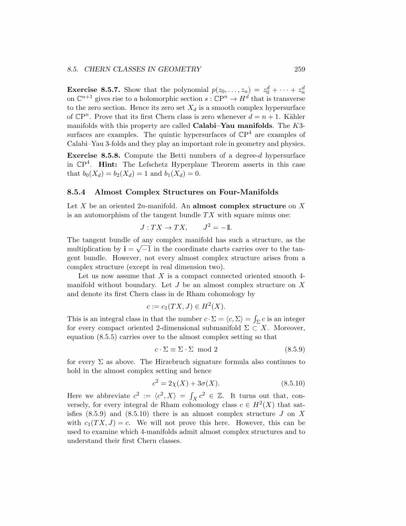
8.5. CHERN CLASSES IN GEOMETRY 259
Exercise 8.5.7. Show that the polynomial p(z0, . . . , zn) = zd0 + · · · + zdnon Cn+1 gives rise to a holomorphic section s : CPn → Hd that is transverseto the zero section. Hence its zero set Xd is a smooth complex hypersurfaceof CPn. Prove that its first Chern class is zero whenever d = n+ 1. Kahlermanifolds with this property are called Calabi–Yau manifolds. The K3-surfaces are examples. The quintic hypersurfaces of CP4 are examples ofCalabi–Yau 3-folds and they play an important role in geometry and physics.
Exercise 8.5.8. Compute the Betti numbers of a degree-d hypersurfacein CP4. Hint: The Lefschetz Hyperplane Theorem asserts in this casethat b0(Xd) = b2(Xd) = 1 and b1(Xd) = 0.
8.5.4 Almost Complex Structures on Four-Manifolds
Let X be an oriented 2n-manifold. An almost complex structure on Xis an automorphism of the tangent bundle TX with square minus one:
J : TX → TX, J2 = −1l.
The tangent bundle of any complex manifold has such a structure, as themultiplication by i =
√−1 in the coordinate charts carries over to the tan-
gent bundle. However, not every almost complex structure arises from acomplex structure (except in real dimension two).
Let us now assume that X is a compact connected oriented smooth 4-manifold without boundary. Let J be an almost complex structure on Xand denote its first Chern class in de Rham cohomology by
c := c1(TX, J) ∈ H2(X).
This is an integral class in that the number c ·Σ = 〈c,Σ〉 =∫
Σ c is an integerfor every compact oriented 2-dimensional submanifold Σ ⊂ X. Moreover,equation (8.5.5) carries over to the almost complex setting so that
c · Σ ≡ Σ · Σ mod 2 (8.5.9)
for every Σ as above. The Hirzebruch signature formula also continues tohold in the almost complex setting and hence
c2 = 2χ(X) + 3σ(X). (8.5.10)
Here we abbreviate c2 := 〈c2, X〉 =∫X c
2 ∈ Z. It turns out that, con-versely, for every integral de Rham cohomology class c ∈ H2(X) that sat-isfies (8.5.9) and (8.5.10) there is an almost complex structure J on Xwith c1(TX, J) = c. We will not prove this here. However, this can beused to examine which 4-manifolds admit almost complex structures and tounderstand their first Chern classes.

260 CHAPTER 8. CONNECTIONS AND CURVATURE
Exercise 8.5.9. Consider the 4-manifold X = CP2#kCP2
(the projectiveplane with k points blown up). This manifold admits a complex structureby a direct construction in algebraic geometry [8]. Verify that it admitsan almost complex structure by finding all integral classes c ∈ H2(X) thatsatisfy (8.5.9) and (8.5.10). Start with k = 0, 1, 2.
Exercise 8.5.10. The k-fold connected sum X = kCP2 = CP2# · · ·#CP2
admits an almost complex structure if and only if k is odd.
Exercise 8.5.11. Which integral class c ∈ H2(T4) is the first Chern classof an almost complex structure on T4.
8.6 Low-Dimensional Manifolds
The examples in the previous section show that there is a rich world ofmanifolds out there whose study is the subject of differential topology andother related areas of mathematics, including complex, symplectic, and alge-braic topology. The present notes only scratch the surface of some of theseareas. One fundamental question in differential topology is how to tell iftwo manifolds of the same dimension m are diffeomorphic, or perhaps notdiffeomorphic as the case may be. In this closing section we discuss someclassical and some more recent answers to this question.
The easiest case is of course m = 1. We have proved in Chapter 2 thatevery compact connected smooth 1-manifold without boundary is diffeomor-phic to the circle and in the case of nonempty boundary is diffeomorphic tothe closed unit interval. We have seen that this observation plays a cen-tral role in the definitions of degree and intersection number, and in factthroughout differential topology.
The next case is m = 2, where this question is also completely un-derstood, although the proof is considerably harder. Two compact con-nected oriented smooth 2-manifolds without boundary are diffeomorphic ifand only if they have the same genus. As pointed out in Example 6.4.14,a beautiful proof of this theorem, based on Morse theory, is contained inthe book of Hirsch [10]. The result generalizes to all compact 2-manifoldswith or without boundary, and orientable or not. Both in the orientableand in the nonorientable case the diffeomorphism type of a compact con-nected 2-manifold is determined by the Euler characteristic and the numberof boundary components. The proof is also contained in [10]. This doesnot mean, however, that the study of 2-manifolds has now been settled. Forexample the study of real 2-manifolds equipped with complex structures

8.6. LOW-DIMENSIONAL MANIFOLDS 261
(called Riemann surfaces) is a rich field of research with connections tomany areas of mathematics such as algebraic geometry, number theory, anddynamical systems. A classical result is the uniformization theorem,which asserts that every connected simply connected Riemann surface isholomorphically diffeomorphic to either the complex plane, or the open unitdisc in the complex plane, or the 2-sphere with its standard complex struc-ture. In particular, it is not necessary to assume that the Riemann surfaceis paracompact; paracompactness is a consequence of uniformization. Thisis a partial answer to a complex analogue of the aforementioned question.We remark that interesting objects associated to oriented 2-manifolds are,for example, the mapping class group (diffeomorphisms up to isotopy) andTeichmuller space (complex structures up to diffeomorphisms isotopic to theidentity).
The compact connected manifolds without boundary in dimensions oneand two are not simply connected except for the 2-sphere. Let us now turnto the higher-dimensional case and focus on simply connected manifolds. Indimension three a central question, which was open for about a century, isthe following.
Three-Dimensional Poincare Conjecture. Every compact connectedsimply connected 3-manifold M without boundary is diffeomorphic to S3.
This conjecture has recently (in the early years of the 21st century) beenconfirmed by Grigory Perelman. His proof is a modification of an earlier pro-gram by Richard Hamilton to use the socalled Ricci flow on the space of allRiemannian metrics on M . The idea is, roughly speaking, to start with anarbitrary Riemannian metric and use it as an initial condition for the Ricciflow. It is then a hard problem in geometry and nonlinear parabolic partialdifferential equations to understand the behavior of the metric under thisflow. The upshot is that, through lot of hard analysis and deep geometricinsight, Perelman succeded in proving that the flow does converge to a roundmetric (with constant sectional curvature). Then a standard result in dif-ferential geometry provides a diffeomorphism to the 3-sphere. The proof ofthe Poincare conjecture is one of the deepest theorems in differential topol-ogy and is an example of the power of analytical tools to settle questionsin geometry and topology. There are now many expositions of Perelman’sproof of the three-dimensional Poincare conjecture, beyond Perelman’s orig-inal papers, too numerous to discuss here. An example is the detailed bookby Morgan and Tian [17].
The higher-dimensional analogue of the the Poincare conjecture assertsthat every compact connected simply connected smooth m-manifold M

262 CHAPTER 8. CONNECTIONS AND CURVATURE
without boundary whose integral cohomology is isomorphic to that of them-sphere, i.e.
Hk(M ;Z) =
Z, for k = 0 and m,0, for 1 ≤ k ≤ m− 1,
is diffeomorphic to the m-sphere. This question is still open in dimen-sion four. However, by the work of Michael Freedman, it is known thatevery such 4-manifold is homeomorphic to the the 4-sphere. In fact onedistingushes between the smooth Poincare conjecture (which assertsthe existence of a diffeomorphism) and the topological Poincare conjec-ture (which asserts the existence of a homeomorphism). Remarkably, thehigher-dimensional Poincare conjecture is much easier to understand thanin dimensions three and four. It was settled long ago by Stephen Smale withthe methods of Morse theory. A beautiful exposition is Milnor’s book [15].The topological Poincare conjecture holds in all dimensions m ≥ 5. But incertain dimensions there are socalled exotic spheres that are homeomor-phic but not diffeomorphic to the m-sphere. Examples are Milnor’s famousexotic 7-spheres. Later work by Kervaire and Milnor showed that there areprecisely 27 exotic spheres in dimension seven.
Let us now turn to compact connected simply connected smooth 4-manifolds X without boundary and with H2(X) 6= 0. The intersection form
QX : H2(X)×H2(X)→ R
is then a diffeomorphism invariant and so are the numbers b+(X) and b−(X)(see Section 8.5.3). They are determined by the Euler characteristic andsignature of X. In fact, more is true. The intersection form can be definedon integral cohomology and Poincare duality over the integers asserts that itremains nondegenerate over the integers (which can be proved with the samemethods as Theorem 6.4.1 once an integral cohomology theory has been setup). This means that it is represented by a symmetric integer matrix withdeterminant ±1 in any integral basis of H2(X;Z).
This leads to the issue of understanding quadratic forms over the inte-gers. One must distinguish between the even and odd case, where evenmeans that Q(a, a) is even for every integer vector a and odd means thatQ(a, a) is odd for some integer vector a. Thus an oriented 4-manifold Xis called even if the self-intersection number of every compact oriented 2-dimensional submanifold Σ ⊂ X without boundary is even and it is calledodd is the self-intersection number is odd for some Σ. This property (beingeven or odd) is called the parity of X. For example, it follows from the
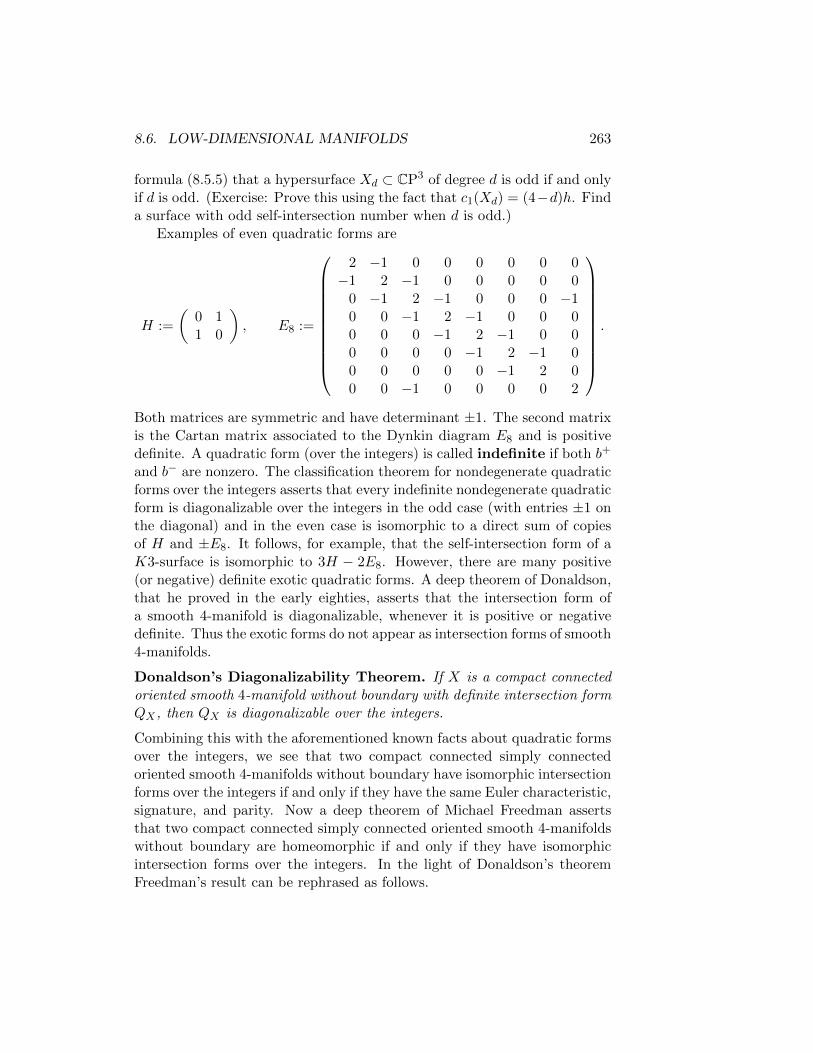
8.6. LOW-DIMENSIONAL MANIFOLDS 263
formula (8.5.5) that a hypersurface Xd ⊂ CP3 of degree d is odd if and onlyif d is odd. (Exercise: Prove this using the fact that c1(Xd) = (4−d)h. Finda surface with odd self-intersection number when d is odd.)
Examples of even quadratic forms are
H :=
(0 11 0
), E8 :=
2 −1 0 0 0 0 0 0−1 2 −1 0 0 0 0 0
0 −1 2 −1 0 0 0 −10 0 −1 2 −1 0 0 00 0 0 −1 2 −1 0 00 0 0 0 −1 2 −1 00 0 0 0 0 −1 2 00 0 −1 0 0 0 0 2
.
Both matrices are symmetric and have determinant ±1. The second matrixis the Cartan matrix associated to the Dynkin diagram E8 and is positivedefinite. A quadratic form (over the integers) is called indefinite if both b+
and b− are nonzero. The classification theorem for nondegenerate quadraticforms over the integers asserts that every indefinite nondegenerate quadraticform is diagonalizable over the integers in the odd case (with entries ±1 onthe diagonal) and in the even case is isomorphic to a direct sum of copiesof H and ±E8. It follows, for example, that the self-intersection form of aK3-surface is isomorphic to 3H − 2E8. However, there are many positive(or negative) definite exotic quadratic forms. A deep theorem of Donaldson,that he proved in the early eighties, asserts that the intersection form ofa smooth 4-manifold is diagonalizable, whenever it is positive or negativedefinite. Thus the exotic forms do not appear as intersection forms of smooth4-manifolds.
Donaldson’s Diagonalizability Theorem. If X is a compact connectedoriented smooth 4-manifold without boundary with definite intersection formQX , then QX is diagonalizable over the integers.
Combining this with the aforementioned known facts about quadratic formsover the integers, we see that two compact connected simply connectedoriented smooth 4-manifolds without boundary have isomorphic intersectionforms over the integers if and only if they have the same Euler characteristic,signature, and parity. Now a deep theorem of Michael Freedman assertsthat two compact connected simply connected oriented smooth 4-manifoldswithout boundary are homeomorphic if and only if they have isomorphicintersection forms over the integers. In the light of Donaldson’s theoremFreedman’s result can be rephrased as follows.

264 CHAPTER 8. CONNECTIONS AND CURVATURE
Freedman’s Theorem. Two compact connected simply connected orientedsmooth 4-manifold without boundary are homeomorphic if and only if theyhave the same Euler characteristic, signature, and parity.
A corollary is the Topological Poincare Conjecture in Dimension Four. Anatural question is if Freedman’s theorem can be strengthened to provide adiffeomorphism. The answer is negative. In the early 1980s, around the sametime when Freedman proved his theorem, Donaldson discovered remarkableinvariants of compact oriented smooth 4-manifolds without boundary bystudying the anti-self-dual Yang–Mills equations with structure group SU(2).He proved that the resulting invariants are nontrivial for Kahler surfaceswhereas they are trivial for every connected sum X1#X2 with b+(Xi) > 0.Thus two such manifolds cannot be diffeomorphic.
Donaldson’s Theorem. Let X be a compact connected simply connectedKahler surface without boundary and assume b+(X) ≥ 2. Then X is not
diffeomorphic to any connected sum kCP2#`CP2.
The only candidate for such a connected sum would be with k = b+(X)and ` = b−(X). Since k ≥ 2, this manifold has trivial Donaldson invariantsand so cannot be diffeomorphic to X. To make the statement interesting wealso have to assume that X is odd. Then the two manifolds are homeomor-phic, by Freedman’s theorem. An infinite sequence of examples is providedby hypersurfaces Xd ⊂ CP3 of odd degree d ≥ 5 (see Section 8.5.3). Theseare connected simply connected Kahler surfaces, satisfy b+(Xd) ≥ 2, andthey are odd. Hence Donaldson’s theorem applies, and Friedmans theorem
furnishes a homeomorphism to a connected sum of CP2’s and CP2’s.
A beautiful introduction to Donaldson theory can be found in the bookby Donaldson and Kronheimer [6]. The book includes a proof of Donald-son’s Diagonalizability Theorem, which is also based on the study of anti-self-dual SU(2)-instantons. When Seiberg–Witten theory was discovered in1994, Taubes proved that all symplectic 4-manifolds have nontrivial Seiberg–Witten invariants. Since the Seiberg–Witten invariants of connected sumshave the same vanishing properties as Donaldson invariants, this gave riseto an extension of Donaldson’s theorem with “Kahler surface” replaced by“symplectic 4-manifold”. Both Donaldson and Seiberg–Witten theory areimportant topics in the study of 3- and 4-manifolds with a wealth of resultsin various directions, the Kronheimer–Mrowka proof of the Thom conjecturebeing just one example (Section 8.5.2). In a nutshell one can think of theseas intersection theories in suitable infinite-dimensional settings. This showsagain the power of analytical methods in topology and geometry.

Appendix A
Notes
This appendix discusses some foundational material that is used through-out this book. Section A.1 examines paracompact topological spaces, Sec-tion A.2 shows how to construct partitions of unity, and Section A.3 showshow to use partitions of unity to embed second countable Hausdorff mani-folds into Euclidean space. Section A.4 explains some background materialabout geodesics and the exponential map that is used in the proof of theTubular Neighborhood Theorem. Section A.5 establishes the classificationof compact one-manifolds following Milnor [14].
A.1 Paracompactness
Definition A.1.1. Let M be a topological space and denote by U ⊂ 2M thecollection of open sets. The topological space M is called
• locally compact if for every open set U ⊂M and every p ∈ U thereexists a compact neighborhood of p that is contained in U ,
• σ-compact if there exists a sequence of compact sets Ki ⊂M suchthat Ki ⊂ int(Ki+1) for all i ∈ N and
⋃∞i=1Ki = M ,
• second countable if its topology has a countable base, i.e. there ex-ists a countable collection of open sets V ⊂ U such that every openset U ∈ U is a union of elements from the collection V ,
• paracompact if every open cover Uαα∈A of M admits a locally fi-nite refinement, i.e. there exists an open cover Vββ∈B such that everyset Vβ is contained in one of the sets Uα and every element p ∈M hasan open neighborhood W such that #β ∈ B |W ∩ Vβ 6= ∅ <∞.
265

266 APPENDIX A. NOTES
We will use the basic facts that a compact subset of a Hausdorff topo-logical space is closed and that a closed subset of a compact set is compact.We will also use the axiom of choice whenever convenient.
Lemma A.1.2. Let M be a locally compact Hausdorff space, let U ⊂M bean open set, and let K ⊂ U be a compact set. Then there exists an openset V ⊂M such that V is compact and
K ⊂ V ⊂ V ⊂ U.
Proof. Since K ⊂ U and M is locally compact, every element p ∈ K has acompact neighborhhod Bp ⊂ U . Since M is a Hausdorff space, the set Bp isclosed. Hence Vp := int(Bp) is an open neighborhood of p such that
p ∈ Vp ⊂ V p ⊂ Bp ⊂ U.
Since Vpp∈K is an open cover of K and K is compact, there exist finitelyelements p1, . . . , p` ∈ K such that
K ⊂ Vp1 ∪ · · · ∪ Vp` =: V.
This set V is open. Its closure V = V p1 ∪ · · · ∪ V p` is a closed subset ofthe compact set B := Bp1 ∪ · · · ∪Bp` and hence is itself compact. More-over, V ⊂ B ⊂ U and this proves Lemma A.1.2.
Lemma A.1.3. Let M be a second countable locally compact Hausdorffspace. Then M is σ-compact.
Proof. Let V be a countable base for the topology of M . Then the collection
Vc := V ∈ V |V is compact
is still a countable base for the topology of M by Lemma A.1.2. Enumeratethe elements of Vc as a sequence
Vc = V1, V2, V3, . . . .
Then, for every k ∈ N, the set Bk := V 1 ∪ · · · ∪ V k is compact and hence iscontained in the set U` := V1 ∪ · · · ∪ V` for some integer ` > k. For k ∈ Nlet ν(k) > k be the smallest integer bigger than k such that Bk ⊂ Uν(k). De-fine the sequence k1 < k2 < k3 < · · · inductively by ki+1 := ν(ki) for i ∈ N.Then
⋃i∈NKi =
⋃k∈N V k = M and, for every i ∈ N, the set Ki := Bki is
compact and contained in Uν(ki) ⊂ int(Ki+1). This proves Lemma A.1.3.

A.1. PARACOMPACTNESS 267
Lemma A.1.4. Let M be a second countable locally compact Hausdorffspace. Then M is paracompact.
Proof. By Lemma A.1.3 there exists a sequence of compact sets Ki ⊂Msuch that
Ki ⊂ int(Ki+1)
for all i ∈ N and ⋃i∈N
Ki = M.
Let Ki := ∅ for i ≤ 0 and, for i ∈ N, define
Bi := Ki \Ki−1, Wi := int(Ki+1) \Ki−2.
Then⋃i∈NBi = M and, for each i ∈ N, the set Bi is compact, the set Wi is
open, and Bi ∩Ki−2 ⊂ Bi ∩ int(Ki−1) = ∅, and so
Bi ⊂Wi, Wi ∩Wi+3 = ∅.
Now let Uαα∈A be an open cover of M . Then, for each i ∈ N, the collection
Wi ∩ Uαα∈A
is an open cover of Bi and so has a finite subcover
Bi ⊂mi⋃j=1
(Wi ∩ Uαij
), αi1, . . . αimi ∈ A.
It follows that the collection
V :=Wi ∩ Uαij | i ∈ N, j = 1, . . . ,mi
is a locally finite refinement of the open cover Uαα∈A of M . Namely,each p0 ∈M belongs to one of the sets Wi0 , and this set intersects only thosesets Wi ∩ Uαij with i0 − 2 ≤ i ≤ i0 + 2. This proves Lemma A.1.4.
We remark that every second countable locally compact Hausdorff spaceis metrizable by the Urysohn Metrization Theorem [19, Thm 34.1]. Usingthis fact one can deduce Lemma A.1.4 from a general theorem which assertsthat every metric space is paracompact [19, Thm 41.4].

268 APPENDIX A. NOTES
A.2 Partitions of Unity
Definition A.2.1. Let M be a smooth manifold. A partition of unityon M is a collection of smooth functions ρα : M → [0, 1], one for each α ∈ A,such that each point p ∈M has an open neighborhood V ⊂M on which onlyfinitely many ρα do not vanish, i.e.
# α ∈ A | ρα|V 6≡ 0 <∞, (A.2.1)
and, for every p ∈M , we have∑α∈A
ρα(p) = 1. (A.2.2)
If Uαα∈A is an open cover of M then a partition of unity ραα∈A (in-dexed by the same set A) is called subordinate to the cover if each ρα issupported in Uα, i.e. supp(ρα) := p ∈M | ρα(p) 6= 0 ⊂ Uα.
Theorem A.2.2 (Partitions of unity). Let M be a smooth manifoldwhose topology is paracompact and Hausdorff. Then, for every open coverof M , there exists a partition of unity subordinate to that cover.
Proof. See page 270.
Corollary A.2.3. Let M be a smooth m-manifold whose topology is para-compact and Hausdorff. Then M admits a Riemannian metric and thetopology on M is metrizable.
Proof. Choose an atlas Uα, φαα∈A on M and let ραα∈A be a partition ofunity, subordinate to the cover Uαα∈A. Then the formula
〈v, w〉 :=∑p∈Uα
ρα(p)〈dφα(p)v, dφα(p)w〉Rm
defines a Riemannian metric on M . To prove that the topology on M ismetrizable, assume first that M is connected. Then the set
Ωp,q := γ : [0, 1]→M | γ is smooth, γ(0) = p, γ(1) = q .
of smooth curves joining p to q is nonempty, and the formula
d(p, q) := infγ∈Ωp,q
L(γ), L(γ) :=
∫ 1
0|γ(t)| dt,
defines a distance function on M . That this distance function induces themanifold topology is proved in [21, Lemma 4.7.1]. If M is disconnected,define d′(p, q) := d(p, q)/(1 + d(p, q)) whenever Ωp,q 6= ∅, and d′(p, q) := 1whenever Ωp,q = ∅. Then d′ : M ×M → [0,∞) is a distance function thatinduces the manifold topology of M . This proves Corollary A.2.3.
A.2. PARTITIONS OF UNITY 269
Lemma A.2.4. Let M be a smooth manifold with a Hausdorff topology.Then, for every open set V ⊂M and every compact set K ⊂ V , there existsa smooth function κ : M → [0,∞) with compact support such that
supp(κ) ⊂ V, κ(p) > 0 for all p ∈ K.
Proof. Assume first that K = p0 is a single point. Since M is a mani-fold it is locally compact. Hence there is a compact neighborhood C ⊂ Vof p0. Since M is Hausdorff C is closed and hence the set U := int(C)is a neighborhood of p0 whose closure U ⊂ C is compact and containedin V . Shrinking U , if necessary, we may assume that there is a coordinatechart φ : U → Ω with values in some open neighborhood Ω ⊂ Rm of theorigin such that φ(p0) = 0. (Here m is the dimension of M .) Now choose asmooth function κ0 : Ω→ [0,∞) with compact support such that κ0(0) > 0.Then the function κ : M → [0, 1], defined by κ|U := κ0 φ and κ(p) := 0for p ∈M \ U is supported in V and satisfies κ(p0) > 0. This proves thelemma in the case where K is a point.
Now let K be any compact subset of V . Then, by the first part ofthe proof, there is a collection of smooth functions κp : M → [0,∞),one for every p ∈ K, such that κp(p) > 0 and supp(κp) ⊂ V . Since Kis compact there are finitely many points p1, . . . , pk ∈ K such that thesets
p ∈M |κpj (p) > 0
cover K. Hence the function κ :=
∑j κpj is sup-
ported in V and is everywhere positive on K. This proves Lemma A.2.4.
Lemma A.2.5. Let M be a topological space. If Vii∈I is a locally finitecollection of open sets in M then⋃
i∈I0
Vi =⋃i∈I0
V i
for every subset I0 ⊂ I.
Proof. The set⋃i∈I0 V i is obviously contained in the closure of
⋃i∈I0 Vi.
To prove the converse choose a point p0 ∈M \⋃i∈I0 V i. Since the collec-
tion Vii∈I is locally finite, there exists an open neighborhood U of p0 suchthat the set I1 := i ∈ I |Vi ∩ U 6= ∅ is finite. Hence the set
U0 := U \⋃
i∈I0∩I1
V i
is an open neighborhood of p0 and we have U0 ∩ Vi = ∅ for every i ∈ I0.Hence p0 /∈
⋃i∈I0 Vi. This proves Lemma A.2.5.

270 APPENDIX A. NOTES
Proof of Theorem A.2.2. Let Uαα∈A be an open cover of M . We prove infour steps that there is a partition of unity subordinate to this cover. Theproofs of steps one and two are taken from [19, Lemma 41.6].
Step 1. There is a locally finite open cover Vii∈I of M such that, forevery i ∈ I, the closure V i is compact and contained in one of the sets Uα.
Denote by V ⊂ 2M the set of all open sets V ⊂M such that V is compactand V ⊂ Uα for some α ∈ A. Since M is a locally compact Hausdorff spacethe collection V is an open cover of M . (If p ∈M then there is an α ∈ A suchthat p ∈ Uα; since M is locally compact there is a compact neighborhoodK ⊂ Uα of p; since M is Hausdorff K is closed and thus V := int(K) is anopen neighborhood of p with V ⊂ K ⊂ Uα.) Since M is paracompact theopen cover V has a locally finite refinement Vii∈I . This cover satisfies therequirements of Step 1.
Step 2. There is a collection of compact sets Ki ⊂ Vi, one for each i ∈ I,such that M =
⋃i∈I Ki.
Denote by W ⊂ 2M the set of all open sets W ⊂ M such that W ⊂ Vi forsome i. Since M is a locally compact Hausdorff space, the collection W is anopen cover of M . Since M is paracompact W has a locally finite refinementWjj∈J . By the axiom of choice there is a map
J → I : j 7→ ij
such that
W j ⊂ Vij ∀ j ∈ J.
Since the collection Wjj∈J is locally finite, we have
Ki :=⋃ij=i
Wj =⋃ij=i
W j ⊂ Vi
by Lemma A.2.5. Since V i is compact so is Ki.
Step 3. There is a partition of unity subordinate to the cover Vii∈I .
Choose a collection of compact sets Ki ⊂ Vi for i ∈ I as in Step 2. Then,by Lemma A.2.4 and the axiom of choice, there is a collection of smoothfunctions κi : M → [0,∞) with compact support such that
supp(κi) ⊂ Vi, κi|Ki > 0 ∀ i ∈ I.

A.2. PARTITIONS OF UNITY 271
Since the cover Vii∈I is locally finite the sum
κ :=∑i∈I
κi : M → R
is locally finite (i.e. each point in M has a neighborhood in which onlyfinitely many terms do not vanish) and thus defines a smooth function on M .This function is everywhere positive, because each summand is nonnegativeand, for each p ∈ M , there is an i ∈ I with p ∈ Ki so that κi(p) > 0. Thusthe funtions χi := κi/κ define a partition of unity satisfying supp(χi) ⊂ Vifor every i ∈ I as required.
Step 4. There is a partition of unity subordinate to the cover Uαα∈A.
Let χii∈I be the partition of unity constructed in Step 3. By the axiomof choice there is a map I → A : i 7→ αi such that Vi ⊂ Uαi for every i ∈ I.For α ∈ A define ρα : M → [0, 1] by
ρα :=∑αi=α
χi.
Here the sum runs over all indices i ∈ I with αi = α. This sum is locallyfinite and hence is a smooth function on M . Moreover, each point in M hasan open neighborhood in which only finitely many of the ρα do not vanish.Hence the sum of the ρα is a well defined function on M and∑
α∈Aρα =
∑α∈A
∑αi=α
χi =∑i∈I
χi ≡ 1.
This shows that the functions ρα form a partition of unity. To prove theinclusion supp(ρα) ⊂ Uα we consider the open sets
Wi := p ∈M |χi(p) > 0
for i ∈ I. Since Wi ⊂ Vi this collection is locally finite. Hence, byLemma A.2.5, we have
supp(ρα) =⋃αi=α
Wi =⋃αi=α
W i =⋃αi=α
supp(χi) ⊂⋃αi=α
Vi ⊂ Uα.
This proves Theorem A.2.2.

272 APPENDIX A. NOTES
A.3 Embedding a Manifold into Euclidean Space
Theorem A.3.1. Let M be a smooth m-manifold whose topology is secondcountable and Hausdorff. Then there exists an embedding f : M → R2m+1
with a closed image.
Proof. The proof has five steps. The first two steps deal with case where Mis compact.
Step 1. Let U ⊂M be an open set and let K ⊂ U be a compact set.Then there exists an integer k ∈ N, a smooth map f : M → Rk, and anopen set V ⊂M , such that K ⊂ V ⊂ U , the restriction f |V : V → Rk is aninjective immersion, and f(p) = 0 for all p ∈M \ U .
Choose a smooth atlas A = (φα, Uα)α∈A on M such that, for each α ∈ A,either Uα ⊂ U or Uα ∩K = ∅. Since M is a paracompact Hausdorff man-ifold, Theorem A.2.2 asserts that there exists a partition of unity ραα∈Asubordinate to the open cover Uαα∈A of M . Since the sets Uα with Uα ⊂ Uform an open cover of K and K is a compact subset of M , there exist finitelymany indices α1, . . . , α` ∈ A such that
K ⊂ Uα1 ∪ · · · ∪ Uα` =: V ⊂ U.
Let k := `(m+ 1) and, for i = 1, . . . , `, abbreviate
φi := φαi , ρi := ραi .
Define the smooth map f : M → Rk by
f(p) :=
ρ1(p)
ρ1(p)φ1(p)...
ρ`(p)ρ`(p)φ`(p)
for p ∈M.
Then the restriction f |V : V → Rk is injective. Namely, if p0, p1 ∈ V satisfy
f(p0) = f(p1)
thenI :=
i∣∣ ρi(p0) > 0
=i∣∣ ρi(p1) > 0
6= ∅
and, for i ∈ I, we have ρi(p0) = ρi(p1), hence φi(p0) = φi(p1), and so p0 = p1.Moreover, for every p ∈ K the derivative df(p) : TpM → Rk is injective, andthis proves Step 1.

A.3. EMBEDDING A MANIFOLD INTO EUCLIDEAN SPACE 273
Step 2. Let f : M → Rk be an injective immersion and let A ⊂ R(2m+1)×k
be a nonempty open set. Then there exists a matrix A ∈ A such that themap Af : M → R2m+1 is an injective immersion.
The proof of Step 2 uses the Theorem of Sard. The sets
W0 :=
(p, q) ∈M ×M∣∣ p 6= q
,
W1 :=
(p, v) ∈ TM∣∣ v 6= 0
are open subsets of smooth second countable Hausdorff 2m-manifolds andthe maps
F0 : A×W0 → R2m+1, F1 : A×W1 → R2m+1,
defined by
F0(A, p, q) := A(f(p)− f(q)), F1(A, p, v) := Adf(p)v
for A ∈ A, (p, q) ∈W0, and (p, v) ∈W1, are smooth. Moreover, the zerovector in R2m+1 is a regular value of F0 because f is injective and of F1
because f is an immersion. Hence it follows from [21, Theorem 2.2.17] thatthe sets
M0 := F−10 (0) =
(A, p, q) ∈ A×W0
∣∣Af(p) = Af(q),
M1 := F−11 (0) =
(A, p, v) ∈ A×W1
∣∣Adf(p)v = 0
are smooth manifolds of dimension
dim(M0) = dim(M1) = (2m+ 1)k − 1.
Since M is a second countable Hausdorff manifold, so are M0 and M1.Hence the Theorem of Sard asserts that the canonical projections
M0 → A : (A, p, q) 7→ A =: π0(A, p, q),
M1 → A : (A, p, v) 7→ A =: π1(A, p, v),
have a common regular value A ∈ A. Since
dim(M0) = dim(M1) < dim(A),
this impliesA ∈ A \ (π0(M0) ∪ π1(M1)) .
Hence Af : M → R2m+1 is an injective immersion and this proves Step 2.
274 APPENDIX A. NOTES
If M is compact, the result follows from Steps 1 and 2 with K = U = M .In the noncompact case the proof requires two more steps to construct anembedding into R4m+4 and a further step to reduce the dimension to 2m+ 1.
Step 3. Assume M is not compact. Then there exists a sequence of opensets Ui ⊂M , a sequence of smooth functions ρi : M → [0, 1], and a sequenceof compact sets Ki ⊂ Ui such that
supp(ρi) ⊂ Ui, Ki = ρ−1i (1) ⊂ Ui, Ui ∩ Uj = ∅
for all i, j ∈ N with |i− j| ≥ 2 and M =⋃∞i=1Ki.
Every manifold is locally compact. Since M is also second countable andHausdorff, Lemma A.1.3 asserts that there exists a sequence of compactsets Ci ⊂M such that Ci ⊂ int(Ci+1) for all i ∈ N and M =
⋃i∈NCi. As in
the proof of Lemma A.1.4 let C0 := ∅ and define
Bi := Ci \ Ci−1 (A.3.1)
for i ∈ N. Then M =⋃i∈NBi. We prove that
Bi = Ci \ int(Ci−1) (A.3.2)
for all i ∈ N. To see this, note first that every compact subset of M is closedbecause M is Hausdorff. Hence the right hand side in (A.3.2) is a closedset containing Ci \ Ci−1 and so Bi ⊂ Ci \ int(Ci−1). To prove the converseinclusion, observe that Ci \Bi ⊂ Ci−1, hence int(Ci) \Bi is an open subsetof Ci−1, hence int(Ci) \Bi ⊂ int(Ci−1), and hence int(Ci) \ int(Ci−1) ⊂ Bi.Since Ci \ int(Ci) ⊂ Ci \ Ci−1 ⊂ Bi by (A.3.1), this proves (A.3.2).
It follows from (A.3.2) that
Bi ⊂Wi := int(Ci+1) \ Ci−2, Wi ∩Bi+2 = ∅ (A.3.3)
for all i. Since the set Bi is compact, the set Wi is open, and M is a locallycompact Hausdorff space, it follows from Lemma A.1.2 by induction thatthere exists a sequence of open sets Ui ⊂M such that
Bi ⊂ Ui ⊂ U i ⊂Wi \ U i−2 (A.3.4)
for all i ∈ N. (Here we take U i−2 = ∅ for i = 1, 2.) Now M is paracom-pact by Lemma A.1.4. Hence it follows from (A.3.4) and Theorem A.2.2that, for each i ∈ N, there exists of a partition of unity subordinate to theopen cover M = Ui ∪ (M \Bi), and hence a smooth function ρi : M → [0, 1]such that supp(ρi) ⊂ Ui and ρi|Bi ≡ 1. Thus Ki := ρ−1
i (1) is a sequenceof compact sets such that Bi ⊂ Ki ⊂ Ui for all i and Ui ∩ Uj = ∅ when-ever |i− j| ≥ 2. Hence M =
⋃i∈NKi and this proves Step 3.

A.3. EMBEDDING A MANIFOLD INTO EUCLIDEAN SPACE 275
Step 4. Assume M is not compact. Then there exists an embedding
f : M → R4m+4
with a closed image and a pair of orthonormal vectors x, y ∈ R4m+4 suchthat, for every ε > 0, there exists a compact set K ⊂M with
supp∈M\K
infs,t∈R
∣∣∣∣ f(p)
|f(p)|− sx− ty
∣∣∣∣ < ε. (A.3.5)
Assume M is not compact and let Ki, Ui, ρi be as in Step 3. Then, bySteps 1 and 2, there exists a sequence of smooth maps gi : M → R2m+1 suchthat gi|M\Ui ≡ 0, the restriction gi|Ki : Ki → R2m+1 is injective, and thederivative dgi(p) : TpM → R2m+1 is injective for all p ∈ Ki and all i ∈ N.Let ξ ∈ R2m+1 be a unit vector and define the maps fi : M → R2m+1 by
fi(p) := ρi(p)
iξ +gi(p)√
1 + |gi(p)|2
(A.3.6)
for p ∈M and i ∈ N. Then the restriction fi|Ki : Ki → R2m+1 is injective,the derivative dfi(p) : TpM → R2m+1 is injective for all p ∈ Ki, and
supp(fi) ⊂ Ui, fi(Ki) ⊂ B1(iξ), fi(M) ⊂ Bi+1(0).
Define the maps fodd, f ev : M → R2m+1 and ρodd, ρev : M → R by
ρodd(p) :=
ρ2i−1(p), if i ∈ N and p ∈ U2i−1,0, if p ∈M \
⋃i∈N U2i−1,
fodd(p) :=
f2i−1(p), if i ∈ N and p ∈ U2i−1,0, if p ∈M \
⋃i∈N U2i−1,
ρev(p) :=
ρ2i(p), if i ∈ N and p ∈ U2i,0, if p ∈M \
⋃i∈N U2i,
f ev(p) :=
f2i(p), if i ∈ N and p ∈ U2i,0, if p ∈M \
⋃i∈N U2i,
and define the map f : M → R4m+4 by
f(p) :=(ρodd(p), fodd(p), ρev(p), f ev(p)
)for p ∈M .

276 APPENDIX A. NOTES
We prove that f is injective. To see this, note that
p ∈ K2i−1 =⇒
2i− 2 <∣∣fodd(p)
∣∣ < 2i,|f ev(p)| < 2i+ 1,
p ∈ K2i =⇒
2i− 1 < |f ev(p)| < 2i+ 1,∣∣fodd(p)∣∣ < 2i+ 2,
(A.3.7)
Now let p0, p1 ∈M such that f(p0) = f(p1). Assume first that p0 ∈ K2i−1.Then ρodd(p1) = ρodd(p0) = 1 and hence p1 ∈
⋃j∈NK2j−1. By (A.3.7), we
also have 2i− 2 < |fodd(p1)| = |fodd(p0)| < 2i and hence p1 ∈ K2i−1. Thisimplies f2i−1(p1) = fodd(p1) = fodd(p0) = f2i−1(p0) and so p0 = p1. Nowassume p0 ∈ K2i. Then ρev(p1) = ρev(p0) = 1 and hence p1 ∈
⋃j∈NK2j .
By (A.3.7), we also have 2i− 1 < |f ev(p1)| = |f ev(p0)| < 2i+ 1, so p1 ∈ K2i,which implies f2i(p1) = f ev(p1) = f ev(p0) = f2i(p0), and so again p0 = p1.This shows that f is injective. That f is an immersion follows from the factthat the derivative dfi(p) is injective for all p ∈ Ki and all i ∈ N.
We prove that f is proper and has a closed image. Let (pν)ν∈N be asequence in M such that the sequence (f(pν))ν∈N in R4m+4 is bounded.Choose i ∈ N such that |fodd(pν)| < 2i and |f ev(pν)| < 2i+ 1 for all ν ∈ N.Then pν ∈
⋃2ij=1Kj for all ν ∈ N by (A.3.7). Hence (pν)ν∈N has a convergent
subsequence. Thus f : M → R4m+4 is an embedding with a closed image.Next consider the pair of orthonormal vectors
x := (0, ξ, 0, 0), y := (0, 0, 0, ξ)
in R4m+4 = R× R2m+1 × R× R2m+1. Let (pν)ν∈N be a sequence in Mthat does not have a convergent subsequence and choose a sequence iν ∈ Nsuch that pν ∈ K2iν−1 ∪ K2iν for all ν ∈ N. Then iν tends to infinity.If pν ∈ K2iν−1 for all ν, then we have lim supν→∞|fodd(pν)|−1|f ev(pν)| ≤ 1by (A.3.7). Passing to a subsequence, still denoted by (pν)ν∈N, we mayassume that the limit λ := limν→∞|fodd(fν)|−1|f ev(pν)| exists. Then
0 ≤ λ ≤ 1, limν→∞
∣∣fodd(pν)∣∣
|f(pν)|=
1√1 + λ2
, limν→∞
|f ev(pν)||f(pν)|
=λ√
1 + λ2,
and it follows from (A.3.6) that
limν→∞
fodd(pν)
|fodd(pν)|= ξ, lim
ν→∞
f ev(pν)
|fodd(pν)|= λξ.
This implies
limν→∞
f(pν)
|f(pν)|=
(0,
ξ√1 + λ2
, 0,λξ√
1 + λ2
)=
1√1 + λ2
x+λ√
1 + λ2y.

A.3. EMBEDDING A MANIFOLD INTO EUCLIDEAN SPACE 277
Similarly, if pν ∈ K2iν for all ν, there exists a subsequence such that thelimit λ := limν→∞|f ev(pν)|−1|fodd(pν)| exists and, by (A.3.6), this implies
limν→∞
f(pν)
|f(pν)|=
(0,
λξ√1 + λ2
, 0,ξ√
1 + λ2
)=
λ√1 + λ2
x+1√
1 + λ2y.
This shows that the vectors x and y satisfy the requirements of Step 4.
Step 5. There exists an embedding f : M → R2m+1 with a closed image.
For compact manifolds the result was proved in Steps 1 and 2 and for m = 0the assertion is obvious, because then M is a finite or countable set withthe discrete topology. Thus assume that M is not compact and m ≥ 1.Choose f : M → R4m+4 and x, y ∈ R4m+4 as in Step 4 and define
A :=
A ∈ R(2m+1)×(4m+4)
∣∣∣∣∣ the vectors Ax and Ayare linearly independent
.
Since m ≥ 1, this is a nonempty open subset of R(2m+1)×(4m+4). We provethat the map Af : M → R2m+1 is proper and has a closed image for ev-ery A ∈ A. To see this, fix a matrix A ∈ A. Let (pν)ν∈N be a sequence in Mthat does not have a convergent subsequence. Then by Step 4 there exists asubsequence, still denoted by (pν)ν∈N, and real numbers s, t ∈ R such that
s2 + t2 = 1, limν→∞
f(pν)
|f(pν)|= sx+ ty, lim
ν→∞|f(pν)| =∞.
This implies
limν→∞
Af(pν)
|f(pν)|= sAx+ tAy 6= 0
and hence limν→∞ |Af(pν)| =∞. Thus the preimage of every compact sub-set of R2m+1 under the map Af : M → R2m+1 is a compact subset of M ,and hence Af is proper and has a closed image.
Now it follows from Step 2 that there exists a matrix A ∈ A such that themap Af : M → R2m+1 is an injective immersion. Hence it is an embeddingwith a closed image. This proves Step 5 and Theorem A.3.1.
The Whitney Embedding Theorem asserts that every second count-able Hausdorff m-manifold M admits an embedding f : M → R2m. Theproof is based on the Whitney Trick and goes beyond the scope of thisbook. The next exercise shows that Whitney’s theorem is sharp.
Remark A.3.2. The manifold RP2 cannot be embedded into R3. The sameis true for the Klein bottle K := R2/ ≡ where the equivalence relation isgiven by [x, y] ≡ [x+ k, `− y] for x, y ∈ R and k, ` ∈ Z.

278 APPENDIX A. NOTES
A.4 The Exponential Map

A.5. CLASSIFYING SMOOTH ONE-MANIFOLDS 279
A.5 Classifying Smooth One-Manifolds
Theorem A.5.1. Every nonempty compact connected smooth one-manifoldis diffeomorphic either to the unit circle S1 = z ∈ C | |z| = 1 or to the unitinterval I = [0, 1] = t ∈ R | 0 ≤ t ≤ 1.
Proof.

280 APPENDIX A. NOTES

Bibliography
[1] Ralph Abraham, Joel W. Robbin, Transversal Mappings and Flows. Benjamin Press, 1967.
[2] Raoul Bott, Loring W. Tu, Differential Forms in Algebraic Topology. Graduate Texts inMathematics, 82. Springer, 1982.
[3] L.E.J.. Brouwer, Uber Abbildungen von Mannigfaltigkeiten. Mathematische Annalen 71(1912), 97–115.
[4] A.B. Brown, Functional Dependence. Transactions of the AMS 38 (1935), 379–394.
[5] Theo Buhler & Dietmar Salamon, Functional Analysis. AMS Graduate Studies in Mathe-matics, 2018.
[6] Simon K. Donaldson, Peter B. Kronheimer The Geometry of Four-Manifolds. Oxford Uni-versity Press, 1990.
[7] A.Ya. Dubovitskii, On differentiable mappings of an n-dimensional cube into a k-dimensionalcube. Mat. Sbornik N.S. 32(74) (1953), 443–464.
[8] Phillip Griffiths, Joseph Harris, Principles of Algebraic Geometry. John Wiley & Sons, 1978.
[9] Victor Guillemin, Alan Pollack, Differential Topology. Prentice-Hall, 1974.
[10] Morris W. Hirsch, Differential Topology. Springer, 1994.
[11] John L. Kelley, General Topology. Graduate Texts in Mathematics, 27. Springer, 1975.
[12] Peter B. Kronheimer, Tomasz Mrowka, Embedded surfaces and the structure of Donaldson’spolynomial invariants. J. Diff. Geom. 41 (1995), 573–734.
[13] Peter B. Kronheimer, Tomasz Mrowka, Monopoles and Three-Manifolds. Cambridge Uni-versity Press 2008.
[14] John W. Milnor, Topology from the Differentible Viewpoint. The University Press ofVorginia, 1969.
[15] John W. Milnor, Lectures on the h-Cobordism Theorem. Princeton University Press, 1965.
[16] John W. Milnor, James D Stasheff Characteristic Classes. Princeton University Press, 1974.
[17] John W. Morgan, Gang Tian, Ricci Flow and the Poincare Conjecture. AMS, 2007.
[18] Anthony P. Morse, The behavior of a function on its critical set. Annals of Mathematics 40(1939), 62–70.
[19] James R. Munkres, Topology, Second Edition. Prentice Hall, 2000.
[20] Peter Ozsvath, Zoltan Szabo, The symplectic Thom conjecture. Ann. of Math. 151 (2000),93–124.
[21] Joel W. Robbin, Dietmar A. Salamon, Introduction to Differential Geometry. ETH, LectureNotes, 28 April 2018. https://people.math.ethz.ch/~salamon/PREPRINTS/diffgeo.pdf
[22] Dietmar A. Salamon, Measure and Integration. EMS, Textbooks in Mathematics, 2016.
[23] Arthur Sard, The measure of the critical values of differentiable maps. Bulletin of the AMS48 (1942), 883–890.
[24] Rene Thom, Quelques proprietes globales des varieetes differentiables. Commentarii Math-ematici Helvetici 28 (1954), 17–86.
[25] A. Tychonoff, Ein Fixpunktsatz. Mathematische Annalen 3 (1935), 767–776.
281

Index
adjunction formula, 250
almost complex structure, 259
alternating k-form, 78
decomposable, 82
pullback, 82
atlas, 5, 16
Betti number, 108
Betti numbers, 145
Bianchi identity, 221
bigraded complex, 160
Brouwer Fixed Point Theorem, 21
Calabi–Yau manifold, 259
Cech
cohomology, 157
complex, 156
Cech–de Rham
cohomology, 161
complex, 161
chain homotopy
equivalence, 115
equivalent, 115
chain map, 115
chain rule, 4, 11
characteristic class, 229
Chern class, 239
Chern polynomial, 240
Clifford torus, 60
codimension, 31
compact support
vertical, 179
complex
curve, 248
manifold, 248
surface, 248
complex line bundle
Hermitian, 239
over CPn, 203
over RP2, 236
over the torus, 236
tautological, 204
complex projective space, 6
connection
complex, 216
flat, 224
Hermitian, 217
on a vector bundle, 208
potential, 209
Riemannian, 216
contractible, 117
coordinate chart, 16
cotangent bundle, 174
covariant derivative, 213
critical point, 12
critical value, 12
cup product, 114
in Cech cohomology, 166
in de Rham cohomology, 91
curvature
of a connection, 219
de Rham cohomology, 91
class dual to a map, 144
282
INDEX 283
class dual to a submanifold, 144compactly supported, 130cup product, 91integral class, 205integral lattice, 205of CPn, 153of Rm, 117of RPm, 154of Tm, 151of Sm, 118vertical compact support, 179with twisted coefficients, 224
de Rham complex, 91de Rham’s Theorem, 168degree
of a differential form, 83of an alternating form, 78
Degree Theorem, 105derivative, 4, 10determinant theorem, 82diffeomorphic, 4diffeomorphism, 4, 9differential form, 83
closed, 91exact, 91with compact support, 83with values in a vector bundle,
207dual bundle, 174
endomorphismof a G-bundle, 214
Euler characteristic, 27, 145Euler class, 198, 232
pullback, 201sum formula, 201
Euler number, 196of the normal bundle, 62
exotic spheres, 262exterior differential, 86, 90
exterior powerof a vector bundle, 175
exterior product, 80of differential forms, 84
fiberof a vector bundle, 172
fixed point, 63index, 63isolated, 63nondegenerate, 63
flat connection, 224Fundamental Theorem
of Algebra, 13, 76
gaugegroup, 222transformation, 222
Gauß map, 27, 96, 107Gauß–Bonnet formula, 108Gaußian curvature, 107G-connection
on a vector bundle, 215genus, 152good cover, 125
finite, 125Grassmannian, 7
Hausdorff space, 8Hermitian
form, 217vector bundle, 217vector space, 217
Hirzebruch Signature Theorem, 255holomorphic
function, 248line bundle, 249section, 249
homotopyequivalence, 116equivalent, 116

284 INDEX
inverse, 116relative, 34
Hopf Lemma, 27horizontal lift
of a curve, 214of a vector field, 226
horizontal subbundle, 224
indefinite quadratic form, 263index
of a nondegenerate zeroof a normal vector field, 55
of a transverse intersection, 45of an isolated intersection, 49of an isolated zero
of a normal vector field, 55of a vector field, 25
integral of a differential form, 92interior product
of a vector field and a differentialform, 97
intersectionform of a 4-manifold, 254index, 45, 49, 52isolated, 49number, 45, 48, 52number modulo two, 40transverse, 31, 32, 48
invariant polynomialon a Lie algebra, 228
inverse function theorem, 11isolated
fixed point, 63intersection, 49zero of a normal vector field, 55zero of a vector field, 25
Jacobian matrix, 4
K3-surface, 258Klein bottle, 277
Lefschetz Fixed Point Theorem, 66Lefschetz Hyperplane Theorem, 256Lefschetz map, 63Lefschetz number, 64, 65, 72
local, 70Lefschetz zeta function, 150Lefschetz–Hopf Theorem, 64Lie derivatine
of a differential form, 97linear complex structure, 82local trivialization, 172locally finite
sum, 271long exact sequence, 121lower semicontinuous, 125
manifoldwith boundary, 16
Mayer–Vietoris sequencefor Ω∗, 120for Ω∗c , 134for H∗, 122for H∗c , 136
Mobius strip, 174Moreau envelope, 125Moser isotopy, 110
nondegeneratefixed point, 63zero of a normal vector field, 55
normal bundle, 53, 176normal vector field, 53
orientablevector bundle, 178
orientedintersection, 44vector bundle, 178
parallel transport, 213parity of a 4-manifold, 262

INDEX 285
partition of unity, 268
subordinate to a cover, 268
Poincare
Conjecture, 261
Poincare conjecture, 9
Poincare duality, 139
Poincare Lemma, 117
Poincare pairing, 139
Poincare–Hopf Theorem, 27
polynomial map, 48
Pontryagin class, 245
proper, 130
pullback
of a connection, 218
of a differential form, 84
of a vector bundle, 175
of an alternating form, 82
pushforward
of a differential form, 179
real projective space, 7
regular point, 12
regular value, 12
relative homotopy, 34
Riemann surface, 261
section
of a vector bundle, 176
along a curve, 213
of the normal bundle, 53
self-intersection number, 52
modulo two, 60
short exact sequence, 121
shuffle, 80
signature
of a 4-manifold, 254
smooth map, 4, 9
star shaped, 125, 187
structure group
of a vector bundle, 172
submanifold, 15with boundary, 19
supportof a differential form, 83
tangent space, 10, 17tangent vector
outward pointing, 17tensor product
of vector bundles, 175Thom class, 184Thom Conjecture, 252Thom form, 183Thom Isomorphism Theorem, 183Thom–Smale transversality, 34–39topological space
Hausdorff, 8torus, 6totally geodesic submanifold, 76transition map, 16, 172transverse, 31
intersection, 31, 32, 48to the zero section, 195
trivial bundle, 174Tubular Neighborhood Theorem, 56Tychonoff Fixed Point Theorem, 21
uniformization, 261unitary group, 217
vector bundle, 172complex, 216homomorphism, 177isomorphic, 177isomorphism, 177of finite type, 183orientable, 178oriented, 178Riemannian, 216with structure group G, 172
vector field

286 INDEX
isolated zero, 25vertical derivative
of a normal vector field, 54of a section, 194
volume form, 109on an oriented Riemannian man-
ifold, 107
Whitney Embedding Theorem, 277Whitney sum
of vector bundles, 175Whitney’s Theorem, 62
zero of a section, 194zero section, 177zero set of a section, 195zeta function
of a dynamical system, 150