introduction to distributed computing with pbdr at the umbc high performance computing facility

Introduction to Distributed Computing with pbdR at the UMBC

High Performance Computing Facility

REU Site: Interdisciplinary Program in High Performance ComputingCenter for Interdisciplinary Research and Consulting

Department of Mathematics and StatisticsUniversity of Maryland, Baltimore County

Andrew M. [email protected]

Last modified: 2013-06-26 14:42

Contents

1 Introduction 2

2 Background 2

3 High Performance Computing at UMBC with tara 33.1 Basics . . . . . . . . . . . . . . . . . . . . . . . . . . . . . . . . . . . . . . . . . . . . . . . 33.2 IMPORTANT: Setting up your environment to use pbdR . . . . . . . . . . . . . . . . . . . 33.3 Serial Hello World with R . . . . . . . . . . . . . . . . . . . . . . . . . . . . . . . . . . . . 4

4 Getting Started with pbdR MPI 54.1 Parallel Hello World . . . . . . . . . . . . . . . . . . . . . . . . . . . . . . . . . . . . . . . 5

4.1.1 Example: Simple Parallel Hello . . . . . . . . . . . . . . . . . . . . . . . . . . . . . 54.1.2 Example: Report Process Information . . . . . . . . . . . . . . . . . . . . . . . . . 64.1.3 Example: Global cat command . . . . . . . . . . . . . . . . . . . . . . . . . . . . . 6

4.2 Point-to-point communication . . . . . . . . . . . . . . . . . . . . . . . . . . . . . . . . . . 84.2.1 Example: Send Matrices . . . . . . . . . . . . . . . . . . . . . . . . . . . . . . . . . 84.2.2 Example: Summing Matrices . . . . . . . . . . . . . . . . . . . . . . . . . . . . . . 9

4.3 Collective communication . . . . . . . . . . . . . . . . . . . . . . . . . . . . . . . . . . . . 94.3.1 Example: Summing Matrices with Reduce . . . . . . . . . . . . . . . . . . . . . . . 104.3.2 Example: Scatter / Gather . . . . . . . . . . . . . . . . . . . . . . . . . . . . . . . 10

4.4 What other MPI communications are available? . . . . . . . . . . . . . . . . . . . . . . . . 13

5 Getting started with Distributed Matrices 135.1 Example: Creating a distributed diagonal matrix . . . . . . . . . . . . . . . . . . . . . . . 135.2 Example: SVD of a distributed matrix . . . . . . . . . . . . . . . . . . . . . . . . . . . . . 155.3 Example: Building a distributed matrix in parallel . . . . . . . . . . . . . . . . . . . . . . 16

6 Statistics Applications 176.1 Monte Carlo Integration . . . . . . . . . . . . . . . . . . . . . . . . . . . . . . . . . . . . . 176.2 Reading Datasets . . . . . . . . . . . . . . . . . . . . . . . . . . . . . . . . . . . . . . . . . 19

6.2.1 Reading on all processes . . . . . . . . . . . . . . . . . . . . . . . . . . . . . . . . . 196.2.2 Broadcasting from one process . . . . . . . . . . . . . . . . . . . . . . . . . . . . . 216.2.3 Reading partitioned data . . . . . . . . . . . . . . . . . . . . . . . . . . . . . . . . 21

6.3 Distributed Regression . . . . . . . . . . . . . . . . . . . . . . . . . . . . . . . . . . . . . . 236.4 Distributed Bootstrap . . . . . . . . . . . . . . . . . . . . . . . . . . . . . . . . . . . . . . 26

1

1 Introduction

pbdR (2012, ”Programming with Big Data in R”) is a recent package for high performance computingin R offered by the Remote Data Analysis and Visualization Center (RDAV) at the National Institutefor Computational Sciences (NICS). pbdR, like its predecessor Rmpi, presents the appealing possibility ofhigh level Message Passing Interface (MPI) programming in the open source math/statistics environmentR. pdbR also supports higher level functionality for distributed dense matrix operations and scalablelinear algebra. We have recently installed pbdR to the cluster tara at the High Performance ComputingFacility (www.umbc.edu/hpcf). In this tutorial, we will demonstrate running pbdR programs through thescheduler on tara and some of the basic capabilities of the software.

This tutorial will assume knowledge of a typical Windows R user — that is, a basic knowledge of theprogramming language and being able to issue commands through the GUI. We will go from this to jobsubmission on the cluster tara, to parallel jobs using pbdR.

The tutorial also assumes the reader has access to the cluster tara. However, most of the materialis not specific to tara. Job submission is shown through the SLURM scheduler (computing.llnl.gov/linux/slurm), but this is open source software and can be obtained for free. pbdR also requires an MPIinstallation which can also be obtained freely.

All programs and datasets discussed in this tutorial are available in a companion tarball namedpbdRtara2013.tar.gz. To extract the contents, use a command such as:

[araim1@tara-fe1 ~]$ tar xvzf pbdRtara2013.tar.gz

2 Background

I learned about pbdR on a trip to Knoxville, TN in March 2013. Its authors were giving a workshopat Univerity of Tennessee, Knoxville. Later in June 2013 I installed the package to tara. I found theinstallation to be straightforward, and that the package itself was a very friendly way to write MPIprograms in R.

The R Project for Statistical Computing (R Core Team, 2013) is arguably the most popular softwarepackage for statistical computing. It is open source, and has a large user community. Users mayextend the software by preparing contributed packages. The Comprehensive R Archive Network (CRAN,cran.r-project.org) is a large archive of contributed R packages, and currently contains over 4600submissions ranging from LASSO regression to MCMC simulation. Programming in R is through asimple and intuitive (in my opinion) high level language, adapted from the S programming language,with rough similarity to Matlab programming.

MPI (Message Passing Interface) is one of the most popular standards for general purpose distributedcomputing; that is, computing which is split and synchronized over multiple computers. MPI programsare traditionally written in lower level languages like C, C++, or FORTRAN. To write an MPI program,one should think from an SPMD (single program multiple data) perspective. There are some number,say np, of MPI processes we control, which are assigned IDs from 0, . . . , np − 1. Otherwise they areall considered equals and all run the same program. The program is written from the perspective of asingle MPI process and tells the process “what is my job?”. An MPI program might specify that certainIDs do something different at certain times. The program also tells the processes when to communicatewith one another. Many problems in statistics are considered “embarassingly parallel”, so that minimalcommunication is needed between processes, and perhaps only at the very end of the computation toproduce (say) a sample average. However, many problems which are interesting from a parallel computingviewpoint exist in statistics, and cannot be solved independently in parallel.

A predecessor to pbdR called Rmpi allows MPI programs to be written in R as well. The documentationin Rmpi seemed to promote a master-slave computing perspective, where one process is responsible forcontrolling the workflow of the others. This seems to go against the spirit of MPI. We found that, on tara,the performance of master-slave computation was inadequate so that a single process Rmpi program wasorders of magnitude slower than a serial R program. It is however possible to run Rmpi in SPMD mode.More information about this can be found on www.umbc.edu/hpcf/resources-tara/how-to-run-R.

html. The author of Rmpi appears to be involved in the development of pbdR. The documentation for

2

www.umbc.edu/hpcf

computing.llnl.gov/linux/slurm

computing.llnl.gov/linux/slurm

cran.r-project.org

www.umbc.edu/hpcf/resources-tara/how-to-run-R.html


pbdR is much more extensive, and the programming interface is easier as well, so pbdR seems preferableto Rmpi.

Another popular R package for parallel computing is called SNOW (Simple Network Of Workstations).SNOW uses a master-slave perspective; the programmer works from the perspective of the master anddistributes computations to available workers. SNOW is probably easier to learn than MPI, but is alsoless expressive. An example of a SNOW command is parSapply, which applies a function to each elementof a vector, and where all such computations are farmed out to available workers. For more informationon using SNOW on tara, see www.umbc.edu/hpcf/resources-tara/how-to-run-R.html. An exhaustivelist of R HPC packages, besides the few noted in this tutorial, is available at cran.r-project.org/web/views/HighPerformanceComputing.html.

As mentioned earlier, the documentation for the pbdR project is fairly extensive. For more informa-tion, good starting places are:

• rdav.nics.tennessee.edu/2012/09/pbdr

• thirteen-01.stat.iastate.edu/snoweye/pbdr

• r-pbd.org

3 High Performance Computing at UMBC with tara

3.1 Basics

UMBC High Performance Computing Facility (HPCF) is the community-based, interdisciplinary corefacility for scientific computing and research on parallel algorithms. See the center’s web page at www.

umbc.edu/hpcf for more information, including:

• Current projects• Publications based on work carried out on the HPCF’s computing clusters• Obtaining an account• How to get started on the computing cluster

The current computing cluster tara is an 86 node machine. Each node features two quad core IntelNehalem X5550 processors (2.66 GHz, 8192 kB cache) and 24 GB of memory. All nodes run the RedhatEnterprise Linux operating system. Attached to the cluster is 160 TB of central storage. For moreinformation, see:

• www.umbc.edu/hpcf/resources-tara/system-description.html

Running programs on an HPC cluster is different than running them on a standard workstation. On acluster, the user typically works on a “head node”. This is where we develop and compile our program.When the program is ready to be run, we submit it to the set of available compute nodes. We don’tspecify directly which compute nodes to use, but instead submit a special script to an entity calledthe scheduler. In the case of tara, the scheduling software is SLURM. The script specifies importantinformation such as how many compute nodes our job will need, how much time it will need to run, howmuch memory, and of course the instructions to run the job itself. The scheduler will check whether therequested resources are available, as there may be many other jobs running on the system. If resourcesare not available, the scheduler will place our job into a queue and allow it to wait. In this tutorial, wewill see some basics of interacting with the scheduler. More information is available at:

• www.umbc.edu/hpcf/resources-tara/how-to-run.html

• www.umbc.edu/hpcf/resources-tara/scheduling-policy.html

• www.umbc.edu/hpcf/resources-tara/how-to-run-R.html

3.2 IMPORTANT: Setting up your environment to use pbdR

Before we begin programming, we need to prepare our R environment. See the section “Using con-tributed libraries” of the web page www.umbc.edu/hpcf/resources-tara/how-to-run-R.html. ThepbdR library won’t load without taking these preliminary steps.

3


cran.r-project.org/web/views/HighPerformanceComputing.html

cran.r-project.org/web/views/HighPerformanceComputing.html

rdav.nics.tennessee.edu/2012/09/pbdr

thirteen-01.stat.iastate.edu/snoweye/pbdr

r-pbd.org

www.umbc.edu/hpcf

www.umbc.edu/hpcf

www.umbc.edu/hpcf/resources-tara/system-description.html

www.umbc.edu/hpcf/resources-tara/how-to-run.html

www.umbc.edu/hpcf/resources-tara/scheduling-policy.html



3.3 Serial Hello World with R

There are several ways to run R programs. Typical R users (especially when using Windows) will startthe R GUI and work interactively. Our goal is to run programs on an HPC cluster which are distributedacross multiple compute nodes. Our first step will be to run R as a batch job through the scheduler. Wewill practice with a Hello World program.

• Although there are GUIs available for R in Linux, typically the R command line is used. Let’s runa program interactively using R command line

[araim1@tara-fe1 interactive]$ R

R version x.xx.x (xxxx-xx-xx)

Copyright (C) xxxx The R Foundation for Statistical Computing

...

> cat("Hello World!\n")

Hello World!

>

• Next we’ll run the program from the Linux command line. We can issue R code, but this getsmessy with more than a few commands.

[araim1@tara-fe1 batch-cmd]$ Rscript -e ’cat("Hello World!\n")’

Hello World!

[araim1@tara-fe1 batch-cmd]$

Or we can run a script.

[araim1@tara-fe1 batch-cmd]$ cat driver.R

cat("Hello World!\n")

[araim1@tara-fe1 batch-cmd]$ Rscript driver.R

Hello World!

[araim1@tara-fe1 batch-cmd]$

• Now let’s try running our program in batch on a compute node using a submission scriptFile: code/hello-serial/batch-scheduler/run1.slurm

1 #!/bin/bash

2 #SBATCH --job-name=helloR

3 #SBATCH --output=slurm.out

4 #SBATCH --error=slurm.err

5 #SBATCH --partition=develop

6

7 # Run a command

8 Rscript -e ’cat("Hello World!\n")’

File: code/hello-serial/batch-scheduler/run2.slurm1 #!/bin/bash

2 #SBATCH --job-name=helloR




6

7 # Run a script

8 Rscript driver.R

[araim1@tara-fe1 batch-scheduler]$ sbatch run1.slurm

Submitted batch job 1327727

[araim1@tara-fe1 batch-scheduler]$ cat slurm.err

[araim1@tara-fe1 batch-scheduler]$ cat slurm.out

Hello World!

[araim1@tara-fe1 batch-scheduler]$

[araim1@tara-fe1 batch-scheduler]$ sbatch run2.slurm


4

[araim1@tara-fe1 batch-scheduler]$ cat slurm.err

[araim1@tara-fe1 batch-scheduler]$ cat slurm.out

Hello World!

[araim1@tara-fe1 batch-scheduler]$

4 Getting Started with pbdR MPI

Now that we’re comfortable running batch R jobs through the scheduler, let’s write some pbdR programs.

4.1 Parallel Hello World

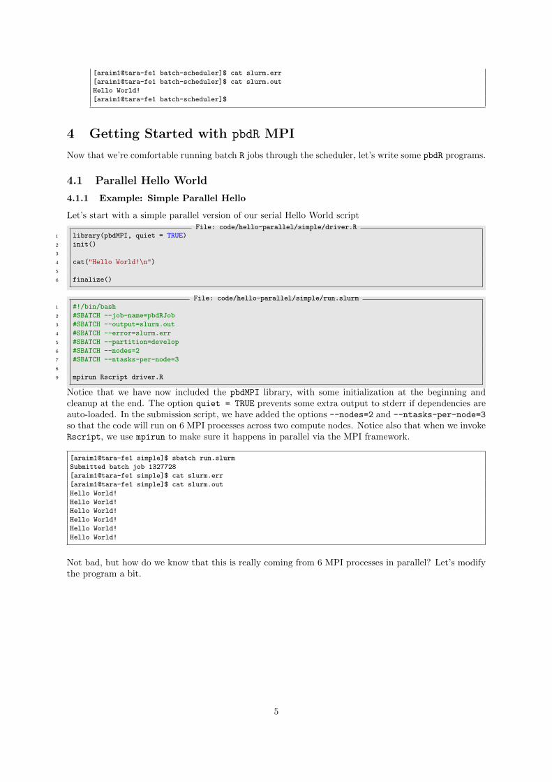
4.1.1 Example: Simple Parallel Hello

Let’s start with a simple parallel version of our serial Hello World scriptFile: code/hello-parallel/simple/driver.R

1 library(pbdMPI, quiet = TRUE)

2 init()

3

4 cat("Hello World!\n")

5

6 finalize()

File: code/hello-parallel/simple/run.slurm1 #!/bin/bash

2 #SBATCH --job-name=pbdRJob




6 #SBATCH --nodes=2

7 #SBATCH --ntasks-per-node=3

8

9 mpirun Rscript driver.R

Notice that we have now included the pbdMPI library, with some initialization at the beginning andcleanup at the end. The option quiet = TRUE prevents some extra output to stderr if dependencies areauto-loaded. In the submission script, we have added the options --nodes=2 and --ntasks-per-node=3

so that the code will run on 6 MPI processes across two compute nodes. Notice also that when we invokeRscript, we use mpirun to make sure it happens in parallel via the MPI framework.

[araim1@tara-fe1 simple]$ sbatch run.slurm


[araim1@tara-fe1 simple]$ cat slurm.err

[araim1@tara-fe1 simple]$ cat slurm.out

Hello World!

Hello World!

Hello World!

Hello World!

Hello World!

Hello World!

Not bad, but how do we know that this is really coming from 6 MPI processes in parallel? Let’s modifythe program a bit.

5

4.1.2 Example: Report Process Information

File: code/hello-parallel/process-id/driver.R1 library(pbdMPI, quiet = TRUE)

2 init()

3 .comm.size <- comm.size()

4 .comm.rank <- comm.rank()

5 .hostname <- Sys.info()["nodename"]

6

7 cat("Hello World from ID", .comm.rank, "on host", .hostname, "of",

8 .comm.size, "processes!\n")

9

10 finalize()

File: code/hello-parallel/process-id/run.slurm1 #!/bin/bash





6 #SBATCH --nodes=2


8


Now we have accessed two very useful MPI variables.

• .comm.size is the number of MPI processes available to our program• .comm.rank is the ID of the current MPI process

In addition, we have also requested the name of the machine which is hosting each process. We havemodified our cat command to print these variables as part of the “hello” greeting. We may use thesame run.slurm script as above for submission, and will continue to use the same script throughout thetutorial unless otherwise noted.

[araim1@tara-fe1 process-id]$ sbatch run.slurm


[araim1@tara-fe1 process-id]$ cat slurm.err

[araim1@tara-fe1 process-id]$ cat slurm.out

Hello World from ID 4 on host n3 of 6 processes!






[araim1@tara-fe1 process-id]$

As an alternative to the cat function, you may prefer sprintf which is useful for formatted printing

> msg <- sprintf("Hello from ID %d on host %s of %d processes!\n", .comm.rank, .hostname, .comm.size)

> cat(msg)

Hello from ID 0 on host n3 of 6 processes!

>

4.1.3 Example: Global cat command

Let’s try one more variation of parallel Hello World using pbdR’s comm.cat function. This is a convenientway to write out text from our group of MPI processes.

6

File: code/hello-parallel/comm-cat/driver.R1 library(pbdMPI, quiet = TRUE)

2 init()




6

7 comm.cat("About to say hello from all processes...\n")

8

9 msg <- sprintf("Hello from ID %d on host %s of %d processes!\n",

10 .comm.rank, .hostname, .comm.size)

11 comm.cat(msg, all.rank = TRUE)

12

13 comm.cat(msg, rank.print = 0)

14 comm.cat(msg, rank.print = 1)

15

16 finalize()

File: code/hello-parallel/comm-cat/run.slurm1 #!/bin/bash





6 #SBATCH --nodes=2


8


Notice that we can control which process prints in comm.cat; we can choose a rank or ask all ranks toprint.

[araim1@tara-fe1 comm-cat]$ sbatch run.slurm


[araim1@tara-fe1 comm-cat]$ cat slurm.err

[araim1@tara-fe1 comm-cat]$ cat slurm.out

COMM.RANK = 0

About to say hello from all processes...

COMM.RANK = 0


COMM.RANK = 1


COMM.RANK = 2


COMM.RANK = 3


COMM.RANK = 4


COMM.RANK = 5


COMM.RANK = 0

About to say hello from some specific processes...

COMM.RANK = 0


COMM.RANK = 1


[araim1@tara-fe1 comm-cat]$

Having the COMM.RANK heading can be useful, but here it is redundant. We can get rid of it with theoption quiet = TRUE

> comm.cat(msg, rank.print = 0, quiet = TRUE)

Hello from ID 0 of 6 processes!

>

7

4.2 Point-to-point communication

Having a bunch of MPI processes running independently is okay, but they’ll need to communicate todo anything really useful. Here we’ll demonstrate point-to-point communication, where processes sendmessages directly to each other.

4.2.1 Example: Send Matrices

File: code/point-to-point-comm/send-matrices/driver.R1 library(pbdMPI, quiet = TRUE)

2 init()



5

6 A <- matrix(.comm.rank, 3, 3)

7

8 if(.comm.rank == 0) {

9 cat("At ID 0, my matrix is:\n")

10 print(A)

11

12 for (id in seq(1, .comm.size-1))

13 {

14 y <- recv(rank.source = id)

15 cat("At ID 0, recv’ed matrix from ID", id, ":\n")

16 print(y)

17 }

18 } else {

19 send(A, rank.dest = 0)

20 }

21

22 finalize()

File: code/point-to-point-comm/send-matrices/run.slurm1 #!/bin/bash





6 #SBATCH --nodes=1


8


In this program, each MPI process creates a 3× 3 matrix A containing its process ID repeated 9 times.Each process sends its copy of A to process 0, who receives them and prints them in order (by processID). Notice that the send and recv commands are used, and an if statement controls the program flow:process 0 does one thing, and all other processes do something else.

Readers familiar with MPI may notice that the send and recv commands have very simple argu-ment lists. We don’t need to specify the number of elements in A being sent, or their type. This ishandled by pbdR. Some options like the MPI communicator have been set to reasonable defaults (i.e.MPI_COMM_WORLD) but may be changed by the user.

[araim1@tara-fe1 send-matrices]$ sbatch run.slurm


[araim1@tara-fe1 send-matrices]$ cat slurm.err

[araim1@tara-fe1 send-matrices]$ cat slurm.out

At ID 0, my matrix is:

[,1] [,2] [,3]

[1,] 0 0 0

[2,] 0 0 0

[3,] 0 0 0

At ID 0, recv’ed matrix from ID 1 :

[,1] [,2] [,3]

[1,] 1 1 1

[2,] 1 1 1

[3,] 1 1 1


[,1] [,2] [,3]

8

[1,] 2 2 2

[2,] 2 2 2

[3,] 2 2 2


[,1] [,2] [,3]

[1,] 3 3 3

[2,] 3 3 3

[3,] 3 3 3

[araim1@tara-fe1 send-matrices]$

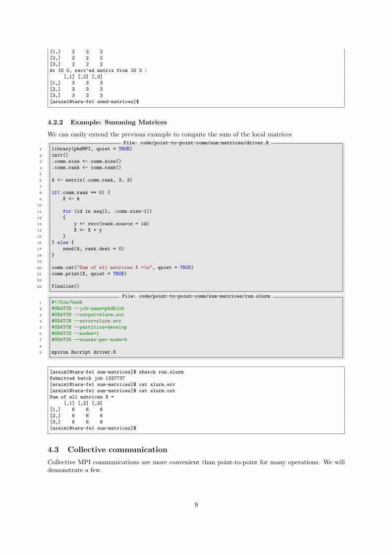
4.2.2 Example: Summing Matrices

We can easily extend the previous example to compute the sum of the local matricesFile: code/point-to-point-comm/sum-matrices/driver.R


2 init()



5


7

8 if(.comm.rank == 0) {

9 X <- A

10

11 for (id in seq(1, .comm.size-1))

12 {

13 y <- recv(rank.source = id)

14 X <- X + y

15 }

16 } else {

17 send(A, rank.dest = 0)

18 }

19

20 comm.cat("Sum of all matrices X =\n", quiet = TRUE)

21 comm.print(X, quiet = TRUE)

22

23 finalize()

File: code/point-to-point-comm/sum-matrices/run.slurm1 #!/bin/bash





6 #SBATCH --nodes=1


8


[araim1@tara-fe1 sum-matrices]$ sbatch run.slurm


[araim1@tara-fe1 sum-matrices]$ cat slurm.err

[araim1@tara-fe1 sum-matrices]$ cat slurm.out

Sum of all matrices X =

[,1] [,2] [,3]

[1,] 6 6 6

[2,] 6 6 6

[3,] 6 6 6

[araim1@tara-fe1 sum-matrices]$

4.3 Collective communication

Collective MPI communications are more convenient than point-to-point for many operations. We willdemonstrate a few.

9

4.3.1 Example: Summing Matrices with Reduce

Here is a more convenient version of the example in section 4.2File: code/collective-comm/reduce-matrix-sum/driver.R


2 init()



5


7 X <- reduce(A, op = "sum")

8

9 comm.print(A, all.rank = TRUE)

10 comm.print(X)

11

12 finalize()

File: code/collective-comm/reduce-matrix-sum/run.slurm1 #!/bin/bash





6 #SBATCH --nodes=1


8


[araim1@tara-fe1 reduce-matrix-sum]$ sbatch run.slurm


[araim1@tara-fe1 reduce-matrix-sum]$ cat slurm.err

[araim1@tara-fe1 reduce-matrix-sum]$ cat slurm.out

COMM.RANK = 0

[,1] [,2] [,3]

[1,] 0 0 0

[2,] 0 0 0

[3,] 0 0 0

COMM.RANK = 1

[,1] [,2] [,3]

[1,] 1 1 1

[2,] 1 1 1

[3,] 1 1 1

COMM.RANK = 2

[,1] [,2] [,3]

[1,] 2 2 2

[2,] 2 2 2

[3,] 2 2 2

COMM.RANK = 3

[,1] [,2] [,3]

[1,] 3 3 3

[2,] 3 3 3

[3,] 3 3 3

COMM.RANK = 0

[,1] [,2] [,3]

[1,] 6 6 6

[2,] 6 6 6

[3,] 6 6 6

[araim1@tara-fe1 reduce-matrix-sum]$

4.3.2 Example: Scatter / Gather

In the following example, we’ll compute an iid sample of 1000 observations from N(µ, σ2) for eachµ ∈ {−10,−9.5, . . . , 9.5, 10}, and return the mean of each sample. To do this, we’ll split the vector(−10,−9.5, . . . , 9.5, 10) into a list of vectors, so that the first vector will be processed by ID 0, thesecond vector will be processed by ID 1, and so forth. Here is the splitting code in serial, assuming that.comm.size has been set to 8.

10

> all.mu.levels <- seq(-10, 10, 0.5)

> idx <- 1:length(all.mu.levels) %% .comm.size

> x <- split(all.mu.levels, idx)

> print(idx)

[1] 1 2 3 4 5 6 7 0 1 2 3 4 5 6 7 0 1 2 3 4 5 6 7 0 1 2 3 4 5 6 7 0 1 2 3 4 5 6

[39] 7 0 1

> print(x)

$‘0‘

[1] -6.5 -2.5 1.5 5.5 9.5

$‘1‘

[1] -10 -6 -2 2 6 10

$‘2‘

[1] -9.5 -5.5 -1.5 2.5 6.5

$‘3‘

[1] -9 -5 -1 3 7

$‘4‘

[1] -8.5 -4.5 -0.5 3.5 7.5

$‘5‘

[1] -8 -4 0 4 8

$‘6‘

[1] -7.5 -3.5 0.5 4.5 8.5

$‘7‘

[1] -7 -3 1 5 9

>

Notice that the jth element of all.mu.levels is assigned to the process with ID ≡ j mod 8. Fromhere, we can use the scatter command so the vectors will be distributed as desired.

File: code/collective-comm/gather-vector/driver.R1 library(pbdMPI, quiet = TRUE)

2 init()



5

6 all.mu.levels <- seq(-10, 10, 0.5)

7 idx <- 1:length(all.mu.levels) %% .comm.size

8 x <- split(all.mu.levels, idx)

9

10 mu.levels <- scatter(split(all.mu.levels, idx))

11 comm.cat("\nAfter scatter, mu.levels:\n", quiet = TRUE)

12 comm.print(mu.levels, all.rank = TRUE)

13

14 m <- numeric( length(mu.levels) )

15 for (i in 1:length(mu.levels))

16 {

17 mu <- mu.levels[i]

18 x <- rnorm(n = 1000, mean = mu, sd = 1)

19 m[i] <- mean(x)

20 }

21

22 means <- gather(m, rank.dest = 0)

23

24 comm.cat("\nOur result on process 0:\n", quiet = TRUE)

25 comm.print(means, quiet = TRUE)

26

27 comm.cat("\nOur result on process 0 after unlist:\n", quiet = TRUE)

28 comm.print(unlist(means), quiet = TRUE)

29

30 finalize()

11

File: code/collective-comm/gather-vector/run.slurm1 #!/bin/bash





6 #SBATCH --nodes=1


8


[araim1@tara-fe1 gather-vector]$ sbatch run.slurm


[araim1@tara-fe1 gather-vector]$ cat slurm.err

[araim1@tara-fe1 gather-vector]$ cat slurm.out

After scatter, mu.levels:

COMM.RANK = 0

[1] -6.5 -2.5 1.5 5.5 9.5

COMM.RANK = 1

[1] -10 -6 -2 2 6 10

COMM.RANK = 2

[1] -9.5 -5.5 -1.5 2.5 6.5

COMM.RANK = 3

[1] -9 -5 -1 3 7

COMM.RANK = 4

[1] -8.5 -4.5 -0.5 3.5 7.5

COMM.RANK = 5

[1] -8 -4 0 4 8

COMM.RANK = 6

[1] -7.5 -3.5 0.5 4.5 8.5

COMM.RANK = 7

[1] -7 -3 1 5 9

Our result on process 0:

[[1]]

[1] -6.526597 -2.485492 1.528951 5.490389 9.460975

[[2]]

[1] -10.026597 -5.985492 -1.971049 1.990389 5.960975 10.045499

[[3]]

[1] -9.526597 -5.485492 -1.471049 2.490389 6.460975

[[4]]

[1] -9.0265972 -4.9854918 -0.9710489 2.9903893 6.9609750

[[5]]

[1] -8.5265972 -4.4854918 -0.4710489 3.4903893 7.4609750

[[6]]

[1] -8.02659720 -3.98549176 0.02895114 3.99038933 7.96097501

[[7]]

[1] -7.5265972 -3.4854918 0.5289511 4.4903893 8.4609750

[[8]]

[1] -7.026597 -2.985492 1.028951 4.990389 8.960975

Our result on process 0 after unlist:

[1] -6.52659720 -2.48549176 1.52895114 5.49038933 9.46097501

[6] -10.02659720 -5.98549176 -1.97104886 1.99038933 5.96097501

[11] 10.04549875 -9.52659720 -5.48549176 -1.47104886 2.49038933

[16] 6.46097501 -9.02659720 -4.98549176 -0.97104886 2.99038933

[21] 6.96097501 -8.52659720 -4.48549176 -0.47104886 3.49038933

[26] 7.46097501 -8.02659720 -3.98549176 0.02895114 3.99038933

[31] 7.96097501 -7.52659720 -3.48549176 0.52895114 4.49038933

[36] 8.46097501 -7.02659720 -2.98549176 1.02895114 4.99038933

[41] 8.96097501

12

[araim1@tara-fe1 gather-vector]$

4.4 What other MPI communications are available?

pbdR does not implement the entire MPI specification, therefore some commands that are available inC and FORTRAN MPI implementations may not be available. However, many MPI commands andoptions are available in pbdR that we have not covered. For more information, see:

• pdbMPI reference manual at: cran.r-project.org/web/packages/pbdMPI• Full MPI specification: www.mpi-forum.org/docs• Quick list of all MPI commands: www.mcs.anl.gov/research/projects/mpi/www/

5 Getting started with Distributed Matrices

pbdR supports higher level programming for distributed dense matrices using the sub-package pbdDMAT.A matrix is distributed among a group of processes using a block-cyclical distribution as in ScaLA-PACK. The details will not be discussed here, but the reader can refer to acts.nersc.gov/scalapack/

hands-on/datadist.html and the package vignette for pbdDMAT at cran.r-project.org/web/packages/pbdDMAT.

5.1 Example: Creating a distributed diagonal matrixFile: code/dmat/diag/driver.R

1 library(pbdDMAT, quiet = TRUE)

2 init.grid()

3

4 Y <- diag(1:6, type = "ddmatrix")

5

6 comm.cat("class of Y on each process:\n", quiet = TRUE)

7 comm.print(class(Y), all.rank = TRUE)

8

9 comm.cat("\nprint:\n", quiet = TRUE)

10 print(Y)

11

12 comm.cat("\nprint with all = TRUE:\n", quiet = TRUE)

13 print(Y, all = TRUE)

14

15 X <- as.matrix(Y, proc.dest = 0)

16 comm.cat("\nConverted to regular matrix:\n", quiet = TRUE)

17 comm.print(X, proc.rank = 0, quiet = TRUE)

18

19 finalize()

File: code/dmat/diag/run.slurm1 #!/bin/bash





6 #SBATCH --nodes=1


8


[araim1@tara-fe1 1]$ sbatch run.slurm


[araim1@tara-fe1 diag]$ cat slurm.err

[araim1@tara-fe1 diag]$ cat slurm.out

Using 1x3 for the default grid size

class of Y on each process:

COMM.RANK = 0

[1] "ddmatrix"

attr(,"package")

13

cran.r-project.org/web/packages/pbdMPI

www.mpi-forum.org/docs

www.mcs.anl.gov/research/projects/mpi/www/

acts.nersc.gov/scalapack/hands-on/datadist.html

acts.nersc.gov/scalapack/hands-on/datadist.html

cran.r-project.org/web/packages/pbdDMAT


[1] "pbdDMAT"

COMM.RANK = 1

[1] "ddmatrix"

attr(,"package")

[1] "pbdDMAT"

COMM.RANK = 2

[1] "ddmatrix"

attr(,"package")

[1] "pbdDMAT"

print:

DENSE DISTRIBUTED MATRIX

---------------------------

@Data: 1e+00, 0e+00, 0e+00, 0e+00, ...

Process grid: 1x3

Global dimension: 6x6

(max) Local dimension: 6x4

Blocking: 4x4

BLACS ICTXT: 0

print with all = TRUE:

dx@Data[ 1, 1]= 1.000000000000000000

dx@Data[ 2, 1]= 0.000000000000000000

dx@Data[ 3, 1]= 0.000000000000000000

dx@Data[ 4, 1]= 0.000000000000000000

dx@Data[ 5, 1]= 0.000000000000000000

dx@Data[ 6, 1]= 0.000000000000000000

dx@Data[ 1, 2]= 0.000000000000000000

dx@Data[ 2, 2]= 2.000000000000000000

dx@Data[ 3, 2]= 0.000000000000000000

...

dx@Data[ 5, 6]= 0.000000000000000000

dx@Data[ 6, 6]= 6.000000000000000000

Converted to regular matrix:

[,1] [,2] [,3] [,4] [,5] [,6]

[1,] 1 0 0 0 0 0

[2,] 0 2 0 0 0 0

[3,] 0 0 3 0 0 0

[4,] 0 0 0 4 0 0

[5,] 0 0 0 0 5 0

[6,] 0 0 0 0 0 6

[araim1@tara-fe1 diag]$

14

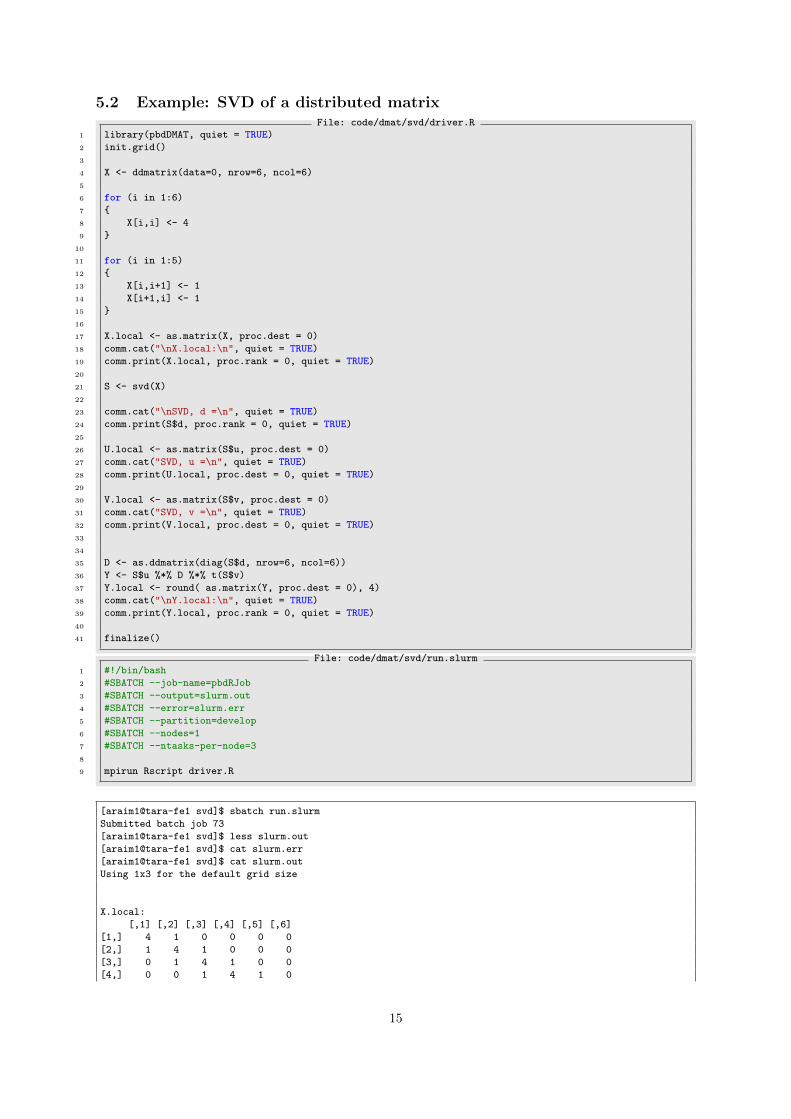
5.2 Example: SVD of a distributed matrixFile: code/dmat/svd/driver.R

1 library(pbdDMAT, quiet = TRUE)

2 init.grid()

3

4 X <- ddmatrix(data=0, nrow=6, ncol=6)

5

6 for (i in 1:6)

7 {

8 X[i,i] <- 4

9 }

10

11 for (i in 1:5)

12 {

13 X[i,i+1] <- 1

14 X[i+1,i] <- 1

15 }

16

17 X.local <- as.matrix(X, proc.dest = 0)

18 comm.cat("\nX.local:\n", quiet = TRUE)

19 comm.print(X.local, proc.rank = 0, quiet = TRUE)

20

21 S <- svd(X)

22

23 comm.cat("\nSVD, d =\n", quiet = TRUE)

24 comm.print(S$d, proc.rank = 0, quiet = TRUE)

25

26 U.local <- as.matrix(S$u, proc.dest = 0)

27 comm.cat("SVD, u =\n", quiet = TRUE)

28 comm.print(U.local, proc.dest = 0, quiet = TRUE)

29

30 V.local <- as.matrix(S$v, proc.dest = 0)

31 comm.cat("SVD, v =\n", quiet = TRUE)

32 comm.print(V.local, proc.dest = 0, quiet = TRUE)

33

34

35 D <- as.ddmatrix(diag(S$d, nrow=6, ncol=6))

36 Y <- S$u %*% D %*% t(S$v)

37 Y.local <- round( as.matrix(Y, proc.dest = 0), 4)

38 comm.cat("\nY.local:\n", quiet = TRUE)

39 comm.print(Y.local, proc.rank = 0, quiet = TRUE)

40

41 finalize()

File: code/dmat/svd/run.slurm1 #!/bin/bash





6 #SBATCH --nodes=1


8


[araim1@tara-fe1 svd]$ sbatch run.slurm


[araim1@tara-fe1 svd]$ less slurm.out

[araim1@tara-fe1 svd]$ cat slurm.err

[araim1@tara-fe1 svd]$ cat slurm.out


X.local:

[,1] [,2] [,3] [,4] [,5] [,6]

[1,] 4 1 0 0 0 0

[2,] 1 4 1 0 0 0

[3,] 0 1 4 1 0 0

[4,] 0 0 1 4 1 0

15

[5,] 0 0 0 1 4 1

[6,] 0 0 0 0 1 4

SVD, d =

[1] 5.801938 5.246980 4.445042 3.554958 2.753020 2.198062

SVD, u =

[,1] [,2] [,3] [,4] [,5] [,6]

[1,] -0.2319206 0.4179065 -0.5211209 0.5211209 -0.4179065 -0.2319206

[2,] -0.4179065 0.5211209 -0.2319206 -0.2319206 0.5211209 0.4179065

[3,] -0.5211209 0.2319206 0.4179065 -0.4179065 -0.2319206 -0.5211209

[4,] -0.5211209 -0.2319206 0.4179065 0.4179065 -0.2319206 0.5211209

[5,] -0.4179065 -0.5211209 -0.2319206 0.2319206 0.5211209 -0.4179065

[6,] -0.2319206 -0.4179065 -0.5211209 -0.5211209 -0.4179065 0.2319206

SVD, v =

[,1] [,2] [,3] [,4] [,5] [,6]

[1,] -0.2319206 0.4179065 -0.5211209 0.5211209 -0.4179065 -0.2319206

[2,] -0.4179065 0.5211209 -0.2319206 -0.2319206 0.5211209 0.4179065

[3,] -0.5211209 0.2319206 0.4179065 -0.4179065 -0.2319206 -0.5211209

[4,] -0.5211209 -0.2319206 0.4179065 0.4179065 -0.2319206 0.5211209

[5,] -0.4179065 -0.5211209 -0.2319206 0.2319206 0.5211209 -0.4179065

[6,] -0.2319206 -0.4179065 -0.5211209 -0.5211209 -0.4179065 0.2319206

Y.local:

[,1] [,2] [,3] [,4] [,5] [,6]

[1,] 4 1 0 0 0 0

[2,] 1 4 1 0 0 0

[3,] 0 1 4 1 0 0

[4,] 0 0 1 4 1 0

[5,] 0 0 0 1 4 1

[6,] 0 0 0 0 1 4

[araim1@tara-fe1 svd]$

5.3 Example: Building a distributed matrix in parallel

For a big data application such as analysis of a large distributed database, the data may not fit on asingle process. Then a natural way to build a distributed matrix will be to have each process contributetheir local piece. Again, more detail is given in the package vignette for pbdDMAT at cran.r-project.

org/web/packages/pbdDMAT.File: code/dmat/build-parallel/driver.R

1 library(pbdDMAT, quiet=TRUE)

2 init.grid()



5

6 newctxt <- minctxt()

7 init.grid(NPROW = 1, NPCOL = .comm.size, ICTXT = newctxt)

8 grid <- blacs(ICTXT = newctxt)

9 .grid.row <- grid$MYROW

10 .grid.col <- grid$MYCOL

11

12 msg <- sprintf("My row is %d and my col is %d\n", .grid.row, .grid.col)

13 comm.cat(msg, all.rank = TRUE)

14

15 x <- matrix(.grid.col, 2, 3)

16 comm.print(x, all.rank = TRUE)

17

18 A <- ddmatrix(data = x, nrow = 2, ncol = 9, bldim = c(2,3), ICTXT = newctxt)

19 print(A)

20 global.A <- as.matrix(A)

21 comm.print(global.A)

22

23 finalize()

16



File: code/dmat/build-parallel/run.slurm1 #!/bin/bash





6 #SBATCH --nodes=1


8


We’ve constructed a 1 × np grid of processes, corresponding to a matrix with 1 × np blocks. Somespecial syntax is needed to create a grid with this configuration (indexed internally by newictxt), andto retrieve information on the grid we just created. Each process retrieves its row and column positionin the grid, and subsequently creates the matrix that will be placed in that position. The distributedmatrix is created by the ddmatrix function. There are some small complications when not all blocks arethe same size; this case is shown in section 6.3.

[araim1@tara-fe1 build-parallel]$ sbatch run.slurm


[araim1@tara-fe1 build-parallel]$ cat slurm.err

[araim1@tara-fe1 build-parallel]$ cat slurm.out


Grid ICTXT=3 of size 1x3 successfully created

COMM.RANK = 0

My row is 0 and my col is 0

COMM.RANK = 1


COMM.RANK = 2


COMM.RANK = 0

[,1] [,2] [,3]

[1,] 0 0 0

[2,] 0 0 0

COMM.RANK = 1

[,1] [,2] [,3]

[1,] 1 1 1

[2,] 1 1 1

COMM.RANK = 2

[,1] [,2] [,3]

[1,] 2 2 2

[2,] 2 2 2


---------------------------

@Data: 0e+00, 0e+00, 0e+00, 0e+00, ...

Process grid: 1x3



Blocking: 2x3

BLACS ICTXT: 3

COMM.RANK = 0

[,1] [,2] [,3] [,4] [,5] [,6] [,7] [,8] [,9]

[1,] 0 0 0 1 1 1 2 2 2

[2,] 0 0 0 1 1 1 2 2 2

6 Statistics Applications

6.1 Monte Carlo Integration

Consider the probability simplex

SJ =

p ∈ [0, 1]J :

J∑j=1

pj = 1

,

17

and let p = (p1, . . . , pJ) follow a DirichletJ(α) distribution on the simplex. Suppose we would like tocompute E(p1 · · · pJ). A simple monte carlo estimator for this quantity is

1

R

R∑r=1

{p(r)1 · · · p

(r)J

}, where p(1), . . . ,p(R) iid∼ DirichletJ(α).

The following pbdR codes compute the monte carlo estimator in serial and parallel with pbdR usingR = 222 repetitions. The parallel program splits the R repetitions among np available processes. Wehave set α = (1, . . . , 1). Table 1 shows a small timing study carried out with this program on tara. Wecan see that varying J from 2 to 10 does not have a large impact on the run time, but for a fixed J , theserial code performs similarly to the pbdR code with one process, and that doubling np halves the runtime. This near-ideal behavior is expected given the embarassingly parallel nature of this problem.

Note that before running this program, you may need to install the MCMCpack library to your account.This can be done by running the following command.

> install.packages("MCMCpack")

File: code/monte-carlo/serial.R1 library(MCMCpack)

2

3 start.time <- Sys.time()

4

5 # Read J and R from the command line, e.g.

6 # Rscript driver.R 2 1048576

7 cmd <- commandArgs(TRUE)

8 J <- as.integer(cmd[1])

9 R <- as.integer(cmd[2])

10

11 alpha <- rep(1,J)

12 n <- R

13

14 # Don’t sample them all at once, or we might run out of memory

15 r <- 0

16 total <- 0

17 while (r < n)

18 {

19 X <- rdirichlet( min(1000, n-r), alpha)

20 total <- total + sum( apply(X, 1, prod) )

21 r <- r + nrow(X)

22 }

23

24 prob.mc <- total / R

25

26 cat("Monte carlo probability:\n")

27 print(prob.mc, digits = 20)

28

29 elapsed <- as.numeric(Sys.time() - start.time, units = "secs")

30 cat("Elapsed secs:", elapsed, "\n")

18

File: code/monte-carlo/driver.R1 library(pbdMPI, quiet = TRUE)

2 library(MCMCpack)

3 init()

4

5 start.time <- Sys.time()

6




10

11 msg <- sprintf("Process ID %d out of %d processes running on %s\n",

12 .comm.rank, .comm.size, .hostname)

13 comm.cat(msg, all.rank = TRUE, quiet = TRUE)

14

15 # Read J and R from the command line, e.g.

16 # Rscript driver.R 2 1048576

17 cmd <- commandArgs(TRUE)

18 J <- as.integer(cmd[1])

19 R <- as.integer(cmd[2])

20

21 alpha <- rep(1,J)

22 n <- R / .comm.size

23

24 # Don’t sample them all at once, or we might run out of memory

25 r <- 0

26 total <- 0

27 while (r < n)

28 {

29 X <- rdirichlet( min(1000, n-r), alpha)

30 total <- total + sum( apply(X, 1, prod) )

31 r <- r + nrow(X)

32 }

33

34 prob.global <- reduce(total / R, op = "sum", rank.dest = 0)

35

36 comm.cat("Monte carlo probability:\n", quiet = TRUE)

37 comm.print(prob.global, digits = 20, quiet = TRUE)

38

39 elapsed <- as.numeric(Sys.time() - start.time, units = "secs")

40 comm.cat("Elapsed secs:", elapsed, "\n", quiet = TRUE)

41

42 finalize()

Here is an example of the submission script; of course the settings for J , --nodes, and --ntasks-per-node

must be changed for each entry of the performance study.File: code/monte-carlo/run.slurm

1 #!/bin/bash





6 #SBATCH --nodes=1


8

9 mpirun Rscript driver.R 4 4194304

6.2 Reading Datasets

Real statistical applications involve data, and therefore it’s worth considering some different ways toread a data file into a parallel R program.

6.2.1 Reading on all processes

The easiest and most obvious thing to do is read the data on all processes. If there are many processesand a large amount of data, this can be very wasteful and processes may contend with each other foraccess to I/O devices.

19

Table 1: Monte Carlo timing study. Entries are elapsed seconds used to compute the approximation.The serial column represents the serial code, while the np columns represent the pbdR code with npprocesses. All runs with 8 processes used a single node, while those with 16 processes used two nodes,and those with 32 processes used four nodes.

J Serial np=1 np=2 np=4 np=8 np=16 np=322 14.0007 13.9731 7.8291 4.0788 2.2214 1.6099 0.72943 14.9866 14.7969 7.7737 4.3116 2.3701 1.3460 0.96554 16.2859 15.6357 8.3377 4.7176 2.4998 1.3869 0.91515 17.3330 16.6487 8.9406 4.8157 2.5994 1.4578 0.85446 17.8716 18.1040 9.4614 4.9742 2.7160 1.5420 0.92127 18.7773 19.1563 10.0340 4.9283 2.8270 1.7059 1.10078 20.1023 19.6903 10.2211 5.4114 2.9414 1.6890 0.93089 21.6230 20.8582 10.9944 5.6989 3.1924 1.8046 0.9473

10 22.6599 21.8145 11.4868 5.9748 3.2320 1.7895 1.0265

File: code/read-data/all-read/driver.R1 library(pbdMPI, quiet = TRUE)

2 init()



5

6 dat <- read.table("../../../data/HondaOdysseyData.csv", sep = ",", head = TRUE)

7 comm.print(dat, all.rank = TRUE)

8

9 finalize()

File: code/read-data/all-read/run.slurm1 #!/bin/bash





6 #SBATCH --nodes=1


8


[araim1@tara-fe1 all-read]$ sbatch run.slurm


[araim1@tara-fe1 all-read]$ cat slurm.err

[araim1@tara-fe1 all-read]$ cat slurm.out

COMM.RANK = 0

Model Price Color Mileage Year

1 Honda Odyssey EX 20890 Dark Cherry Pearl 41922 2008

2 Honda Odyssey EX-L 26810 Green 42533 2008

...

100 Honda Odyssey EX-L 23714 Light Blue 29293 2008

COMM.RANK = 1




...


COMM.RANK = 2




...


[araim1@tara-fe1 all-read]$

20

6.2.2 Broadcasting from one process

A better idea is to read the file on one process and broadcast the data to all other processes. Again, thisassumes the data isn’t large, and having np copies won’t be too expensive.

File: code/read-data/process0-read/driver.R1 library(pbdMPI, quiet = TRUE)

2 init()



5

6 dat0 <- NULL

7 if (.comm.rank == 0)

8 {

9 filename <- "../../../data/HondaOdysseyData.csv"

10 dat0 <- read.table(filename, sep = ",", head = TRUE)

11 }

12

13 dat <- bcast(dat0, rank.source = 0)

14 comm.print(dat, all.rank = TRUE)

15

16 finalize()

File: code/read-data/process0-read/run.slurm1 #!/bin/bash





6 #SBATCH --nodes=1


8


araim1@tara-fe1 process0-read]$ sbatch run.slurm


[araim1@tara-fe1 process0-read]$ cat slurm.err

[araim1@tara-fe1 process0-read]$ cat slurm.out

COMM.RANK = 0




...


COMM.RANK = 1




...


COMM.RANK = 2



...


6.2.3 Reading partitioned data

The data may be too large to fit on a single process. Suppose our data file has been partitionedinto three pieces, with 34 rows in the first piece, 34 in the second pieces, and 32 in the third piece.These partitioned files are named HondaOdysseyData_part0.csv, HondaOdysseyData_part1.csv, andHondaOdysseyData_part2.csv respectively. We can use three processes to build a distributed matrixas follows, without a single process ever having to store the combined data.

21

File: code/read-data/partitioned-read/driver.R1 library(pbdDMAT, quiet=TRUE)

2 init.grid()



5

6 # Create a np x 1 grid of processes where we’ll distribute our matrix


8 init.grid(NPROW = .comm.size, NPCOL = 1, ICTXT = newctxt)




12

13 msg <- sprintf("ID %d: My grid position is (%d,%d)\n",

14 .comm.rank, grid$MYROW, grid$MYCOL)


16

17 dd <- "../../../data/"

18 filename <- sprintf("%s/HondaOdysseyData_part%d.csv", dd, .grid.row)

19 dat <- read.table(filename, sep = ",", head = TRUE)

20 X.local <- cbind(dat$Price, dat$Mileage, dat$Year)

21

22 msg <- sprintf("ID %d: Read data file %s\n", .comm.rank, filename)


24 comm.print(X.local, all.rank = TRUE)

25

26 k <- ncol(X.local)

27 l.n <- nrow(X.local)

28 n <- allreduce(l.n, op = ’sum’)

29 blrows <- allreduce(l.n, op = "max")

30

31 X <- new("ddmatrix", Data=X.local, dim=c(n,k), ldim=dim(X.local),

32 bldim=c(blrows,k), ICTXT = newctxt)

33 X <- redistribute(X, bldim=c(4,4))

34

35 print(X)

36 X.global <- as.matrix(X)

37 comm.print(X.global)

38

39 finalize()

File: code/read-data/partitioned-read/run.slurm1 #!/bin/bash





6 #SBATCH --nodes=1


8


This code is a bit more complicated than before. We are again working with a process grid as in section5.3. One (realistic) complication here is that the number of rows is not equal across all pieces of thedata. Notice that the variable blrows, which represents the number of rows in each block, is taken tobe the maximum of the number of rows of the data pieces. The partitioning of the data into 34, 34,and 32 rows (where all blocks are of equal size except for the last block which has the leftovers) hasbeen selected on purpose to be compatible with the matrix blocking format. The distributed matrix isinitially created in a natural way, so that process 0 holds the first set of rows, process 1 holds the secondset, and process 2 holds the third set. This is not an ideal distribution for parallel matrix operations, sowe use redistribute to rearrange the blocking scheme.

One issue that we have avoided is that some of our columns are not numeric. As of right now, pbdRappears not to support distributed data frames or matrices of strings. We have ignored the non-numericcolumns in this example. We may code them into numeric variables, but the coding should be the sameacross all processes, and therefore would require some communication. We show one way to handle thisin section 6.3

[araim1@tara-fe1 partitioned-read]$ sbatch run.slurm

22


[araim1@tara-fe1 partitioned-read]$ cat slurm.err

[araim1@tara-fe1 partitioned-read]$ cat slurm.out



ID 0: My grid position is (0,0)



ID 0: Read data file ../../../data//HondaOdysseyData_part0.csv



COMM.RANK = 0

[,1] [,2] [,3]

[1,] 20890 41922 2008

[2,] 26810 42533 2008

...

[34,] 26846 32210 2008

COMM.RANK = 1

[,1] [,2] [,3]

[1,] 21900 51938 2008

[2,] 29491 20895 2008

...

[34,] 29990 13690 2010

COMM.RANK = 2

[,1] [,2] [,3]

[1,] 27988 46975 2008

[2,] 25900 48479 2008

...

[32,] 23714 29293 2008


---------------------------

@Data: 2.09e+04, 2.68e+04, 2.58e+04, 2.65e+04, ...

Process grid: 1x3



Blocking: 4x4

BLACS ICTXT: 0

COMM.RANK = 0

[,1] [,2] [,3]

[1,] 20890 41922 2008

[2,] 26810 42533 2008

...

[100,] 23714 29293 2008

[araim1@tara-fe1 partitioned-read]$

6.3 Distributed Regression

Now we will extend the example from section 6.2.3 into a distributed regression. Since the dataset isn’tlarge, we can first run the regression in serial and then compare the result with our parallel version.

23

File: code/parallel-regression/serial.R1 filename <- sprintf("../../data/HondaOdysseyData.csv")


3

4 Model.levels <- levels(dat$Model)

5 Year.levels <- levels(as.ordered(dat$Year))

6

7 Price <- dat$Price

8 Model <- factor(dat$Model, levels = Model.levels)

9 Year <- factor(dat$Year, levels = Year.levels)

10 Mileage <- dat$Mileage

11

12 X <- model.matrix(~ Model + Mileage + Year)

13 y <- Price

14

15 beta.hat <- solve(t(X) %*% X) %*% t(X) %*% y

16 cat("beta.hat = \n")

17 print(beta.hat)

Next is the parallel version. Notice that when we code the non-numeric variables into numbers, we needto do some communication so that the coding is the same on all processes.

24

File: code/parallel-regression/driver.R1 library(pbdDMAT, quiet=TRUE)

2 init.grid()



5

6 # Create a np x 1 grid of processes where we’ll distribute our matrix


8 init.grid(NPROW = .comm.size, NPCOL = 1, ICTXT = newctxt)




12

13 msg <- sprintf("ID %d: My grid position is (%d,%d)\n",

14 .comm.rank, .grid.row, .grid.col)


16

17 # ------------ Read data for regression ------------

18 dd <- "../../data"

19 filename <- sprintf("%s/HondaOdysseyData_part%d.csv", dd, .grid.row)


21

22 msg <- sprintf("ID %d: Read data file %s\n", .comm.rank, filename)


24

25 # We need a global coding for factor and ordered variables

26 Model.levels <- unique(unlist(allgather(levels(dat$Model))))

27 Year.levels <- unique(unlist(allgather(levels(as.ordered(dat$Year)))))

28

29 Price <- dat$Price

30 Model <- factor(dat$Model, levels = Model.levels)

31 Year <- factor(dat$Year, levels = Year.levels)

32 Mileage <- dat$Mileage

33

34 # Create a model matrix for the local regressors

35 X.local <- model.matrix(~ Model + Mileage + Year)

36 y.local <- as.matrix(Price)

37

38 # If we don’t clear the dimension names, we get an error later

39 # from redistribute

40 attributes(X.local)$dimnames <- NULL

41

42 # ------------ Create distributed matrices for X and y ------------

43 k <- ncol(X.local)

44 l.n <- nrow(X.local)

45 n <- allreduce(l.n, op = ’sum’)

46 blrows <- allreduce(l.n, op = "max")

47

48 X <- new("ddmatrix", Data=X.local, dim=c(n,k), ldim=dim(X.local),

49 bldim=c(blrows,k), ICTXT = newctxt)

50 y <- new("ddmatrix", Data=y.local, dim=c(n,1), ldim=dim(y.local),

51 bldim=c(blrows,1), ICTXT = newctxt)

52 X <- redistribute(X, bldim=c(4,4))

53 y <- redistribute(y, bldim=c(4,1))

54

55 # ------------ Fit regression in parallel ------------

56 beta.hat <- solve(t(X) %*% X) %*% t(X) %*% y

57

58 comm.cat("beta.hat =\n", quiet = TRUE)

59 global.beta.hat <- as.matrix(beta.hat, proc.dest = ’all’)

60 comm.print(global.beta.hat, quiet = TRUE)

61

62 finalize()

25

File: code/parallel-regression/run.slurm1 #!/bin/bash





6 #SBATCH --nodes=1


8


[araim1@tara-fe1 parallel-regression]$ Rscript serial.R

beta.hat =

[,1]

(Intercept) 26553.1454095

ModelHonda Odyssey EX-L 3480.7120629

ModelHonda Odyssey LX -2243.9049314

ModelHonda Odyssey Touring 6063.8962923

Mileage -0.1199107

Year2009 61.4883089

Year2010 4471.2837923

[araim1@tara-fe1 parallel-regression]$ sbatch run.slurm


[araim1@tara-fe1 parallel-regression]$ cat slurm.err

[araim1@tara-fe1 parallel-regression]$ cat slurm.out






ID 0: Read data file ../../data/HondaOdysseyData_part0.csv



beta.hat =

[,1]

[1,] 26553.1454095

[2,] 3480.7120629

[3,] -2243.9049314

[4,] 6063.8962923

[5,] -0.1199107

[6,] 61.4883089

[7,] 4471.2837923

[araim1@tara-fe1 parallel-regression]$

6.4 Distributed Bootstrap

Distributed computing could also be helpful for the bootstrap algorithm in a large data setting. Supposeagain that our dataset is too large to fit on a single process, but is split into four pieces. Four MPIprocesses will be used to compute the bootstrap in a distributed manner, where each is responsible forone piece of the data. We demonstrate on the law82 dataset which can be found in the bootstrap

package. The bootstrap package can be installed by the following command.

> install.packages("bootstrap")

The goal is to compute the standard error of the sample correlation between the variables LSAT and GPA.This example was adapted from (Rizzo, 2008, Chapter 7). A serial version is given first.

26

File: code/parallel-bootstrap/serial.R1 library(bootstrap)

2 set.seed(1234)

3

4 n <- nrow(law82)

5 B <- 500

6 T.boot <- numeric(B)

7

8 for (b in 1:B)

9 {

10 idx <- sample(1:n, replace = TRUE)

11 LSAT.boot <- law82$LSAT[idx]

12 GPA.boot <- law82$GPA[idx]

13 T.boot[b] <- cor(LSAT.boot, GPA.boot)

14 }

15

16 print(T.boot)

17

18 se.boot <- sd(T.boot)

19 cat("se.boot =", se.boot, "\n")

For our parallel version, process 0 is responsible for drawing the indices which will be included in eachbootstrap sample. These indices are the broadcast to all other processes. Note that if the number ofobservations n was very large, this might not be feasible, and we would have to reconsider doing it ina distributed way. Each process checks bootstrap indices against the list of local observations. Usingthose observations and a parallel inner product function, all processes cooperate to compute the samplecorrelation. After B = 500 bootstap iterations, all processes contain B sample correlations, which theycan then use to compute the standard error.

27

File: code/parallel-bootstrap/driver.R1 library(pbdMPI, quiet = TRUE)

2 init()



5

6 set.seed(1234)

7

8 filename <- sprintf("../../data/law82-%d.dat", .comm.rank)

9 dat <- read.table(filename)

10

11 l.n <- nrow(dat)

12 l.idx <- as.integer(rownames(dat))

13 n <- allreduce(l.n, op = "sum")

14 B <- 500

15 T.boot <- numeric(B)

16

17 inner.prod.mpi <- function(x, y, idx)

18 {

19 # idx are global indices

20 idx <- idx[idx %in% l.idx]

21

22 # jdx are local indices that index into the local data structures

23 jdx <- idx - min(l.idx) + 1

24

25 x.y <- sum(x[jdx] * y[jdx])

26

27 # Just in case this process didn’t receive any indices, use x.y = 0

28 if (is.na(x.y)) { x.y <- 0 }

29

30 x.y <- allreduce(x.y, op = "sum")

31 return(x.y)

32 }

33

34 cor.mpi <- function(x, y, idx)

35 {

36 # Compute the means for the current bootstrap sample given by idx

37 # and subtract the means from the data

38 ones <- matrix(1/n, nrow = n, ncol = 1)

39 m.x <- inner.prod.mpi(x, ones, idx)

40 m.y <- inner.prod.mpi(y, ones, idx)

41 x <- x - m.x

42 y <- y - m.y

43

44 # Compute the correlation

45 x.y <- inner.prod.mpi(x, y, idx)

46 x.x <- inner.prod.mpi(x, x, idx)

47 y.y <- inner.prod.mpi(y, y, idx)

48

49 r <- x.y / ( sqrt(x.x) * sqrt(y.y) )

50 return(r)

51 }

52

53 for (b in 1:B)

54 {

55 idx0 <- NULL

56 if (.comm.rank == 0)

57 {

58 idx0 <- as.matrix( sample(1:n, replace = TRUE) )

59 }

60

61 idx <- bcast(idx0, rank.source = 0)

62 T.boot[b] <- cor.mpi(dat$LSAT, dat$GPA, idx)

63 }

64

65 comm.cat("T.boot:\n", quiet = TRUE)

66 comm.print(T.boot)

67

68 se.boot <- sd(T.boot)

69 comm.cat("se.boot =", se.boot, "\n", quiet = TRUE)

70

71 finalize()

28

File: code/parallel-bootstrap/run.slurm1 #!/bin/bash




5 #SBATCH --partition=batch

6 #SBATCH --nodes=1


8


[araim1@tara-fe1 parallel-bootstrap]$ Rscript serial.R

[1] 0.7481419 0.6826217 0.7372387 0.7866147 0.7143817 0.8205919 0.7622383

...

[498] 0.7054161 0.6987140 0.6776666

se.boot = 0.05323558

[araim1@tara-fe1 parallel-bootstrap]$ sbatch run.slurm


[araim1@tara-fe1 parallel-bootstrap]$ cat slurm.err

[araim1@tara-fe1 parallel-bootstrap]$ cat slurm.out

T.boot:

COMM.RANK = 0

[1] 0.7481419 0.6826217 0.7372387 0.7866147 0.7143817 0.8205919 0.7622383

...

[498] 0.7054161 0.6987140 0.6776666

se.boot = 0.05323558

[araim1@tara-fe1 parallel-bootstrap]$

Acknowledgements

Thanks to Dr. George Ostrouchov at Oak Ridge National Labratory for his invitation, as well as forarranging financial support from the NICS Remote Data and Visualization Center (funded by NSF),allowing the author to attend the NICS training event in March 2013 and gain exposure to pbdR. Sections5.3, 6.2, 6.3, and 6.4 of this document were suggested by Dr. Nagaraj Neerchal after a two hour workshop(“Introduction to pbdR with tara @ HPCF”) which was held on 6/16/2013. Thanks to all attendees ofthis workshop for their participation and helpful feedback.

The hardware used in this tutorial is part of the UMBC High Performance Computing Facility(HPCF). The facility is supported by the U.S. National Science Foundation through the MRI program(grant nos. CNS–0821258 and CNS–1228778) and the SCREMS program (grant no. DMS–0821311),with additional substantial support from the University of Maryland, Baltimore County (UMBC). Seewww.umbc.edu/hpcf for more information on HPCF and the projects using its resources. The authoradditionally acknowledges financial support as HPCF RA.

References

G. Ostrouchov, W.-C. Chen, D. Schmidt, and P. Patel. Programming with Big Data in R, 2012. URLhttp://r-pbd.org.

R Core Team. R: A Language and Environment for Statistical Computing. R Foundation for StatisticalComputing, Vienna, Austria, 2013. URL http://www.R-project.org.

Maria L. Rizzo. Statistical Computing with R. Chapman & Hall/CRC, 2008.

29

www.umbc.edu/hpcf

http://r-pbd.org

http://www.R-project.org

introduction to distributed computing with pbdr at the umbc high performance computing facility

Documents