introduction to dna microarray data - mathematics and...

Introduction to DNA Microarray Data

Longhai Li

Department of Mathematics and Statistics

University of Saskatchewan

Saskatoon, SK, CANADA

Workshop “Statistical Issues in Biomarker and Drug Co-development”

Fields Institute in Toronto

7 November 2014

Introduction to DNA Microarray Data 2/44

Acknowledgements

● Thanks to the workshop organization committee for providing this great opportunity to meet so many great researchers.

● Thanks to NSERC and CFI for financial supports.


Outline

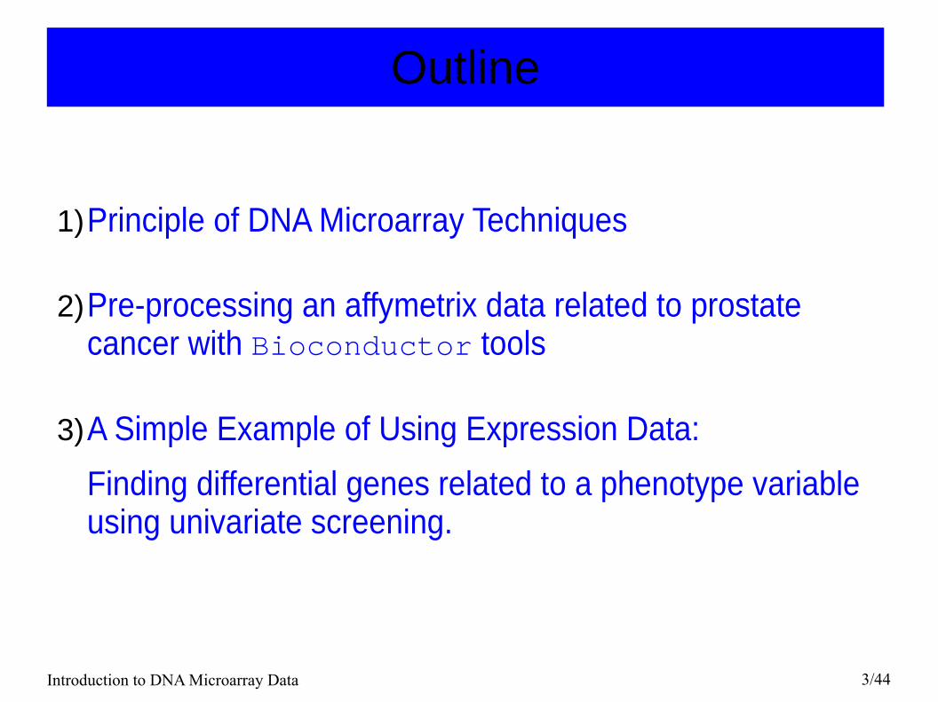
1)Principle of DNA Microarray Techniques

2)Pre-processing an affymetrix data related to prostate cancer with Bioconductor tools

3)A Simple Example of Using Expression Data:

Finding differential genes related to a phenotype variable using univariate screening.


Part I

Principle of DNA Microarray Techniques


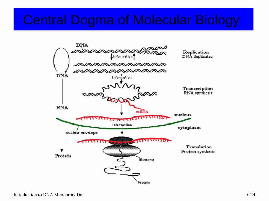
Central Dogma of Molecular Biology The genetic information is stored in the DNA molecules. When the cells are producing proteins, the expression of genetic information occurs in two stages:

1) transcription, during which DNA is transcribed into mRNA

2) translation, during which mRNA is translated to produce proteins.

DNA -> mRNA -> protein

During this process, there are other important aspects of regulation, such as methylation, alternative splicing, which controls which genes are transcribed in different cells.


Central Dogma of Molecular Biology


Transcriptome

● To investigate activities in different cells, we could measure protein levels. However, this is still very difficult.

● Alternatively, we can measure the abundance of all mRNAs (transcriptome) in cells. mRNA or transcript abundance sensitively reflect the state of a cell:

– Tissue source: cell type, organ.– Tissue activity and state:

● Stage of cell development, growth, death. ● Cell cycle.● Disease or normal.● Response to therapy, stress.


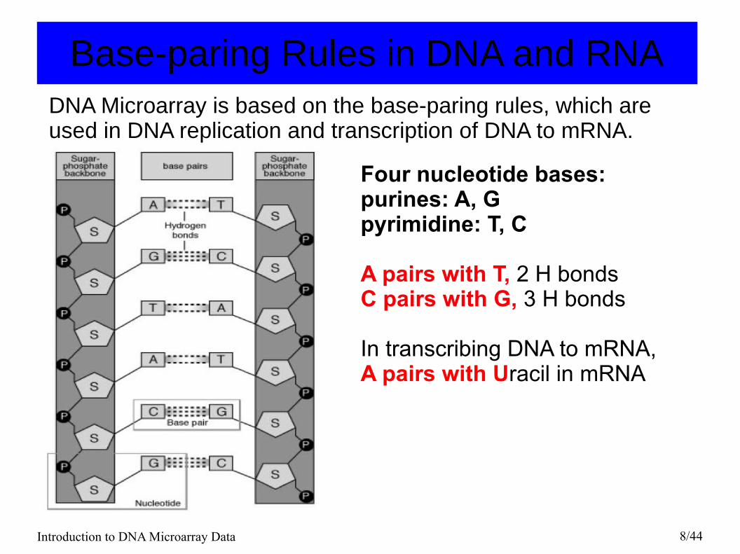
Base-paring Rules in DNA and RNA

Four nucleotide bases: purines: A, Gpyrimidine: T, C

A pairs with T, 2 H bonds C pairs with G, 3 H bonds

In transcribing DNA to mRNA, A pairs with Uracil in mRNA

DNA Microarray is based on the base-paring rules, which are used in DNA replication and transcription of DNA to mRNA.


Hybridization

● We can use DNA single strands to make probes representing different genes.

● In principle, the mRNA that complements a probe sequence by the base-paring rules will be more likely to bind (or hybridize) to the probe.

● We measure mRNA levels of a sample by looking at the hybridization levels to different probes.


Hybridization


Types of Gene Expression Assays

The main types of gene expression assays:● Serial analysis of gene expression (SAGE);● Short oligonucleotide arrays (Affymetrix);● Long oligonucleotide arrays (Agilent Inkjet); ● Fibre optic arrays (Illumina);● Spotted cDNA arrays (Brown/Botstein).● RNA-seq.


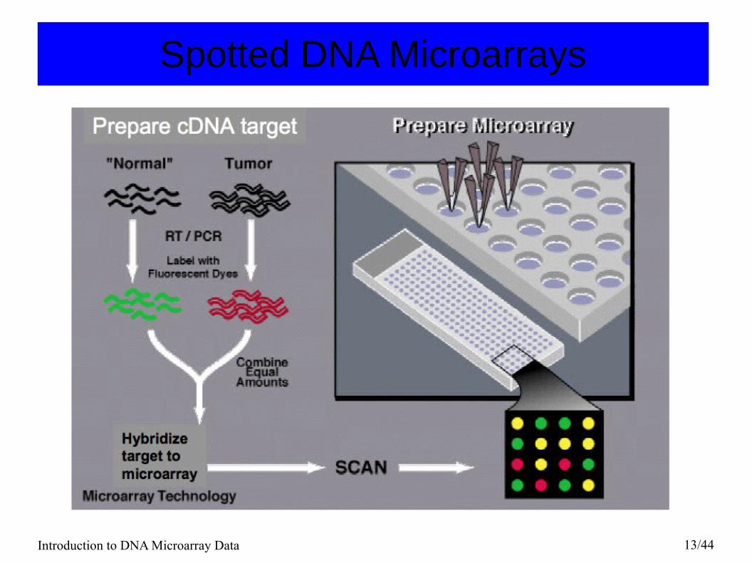
Spotted DNA Microarrays

● Probes: DNA sequences spotted on the array● Targets: Fluorescent cDNA samples synthesized from

mRNA samples following base-paring rules.● The ratio of the red and green fluorescence intensities for

each spot is indicative of the relative abundance of the corresponding DNA probe in the two nucleic acid target samples.


Spotted DNA Microarrays


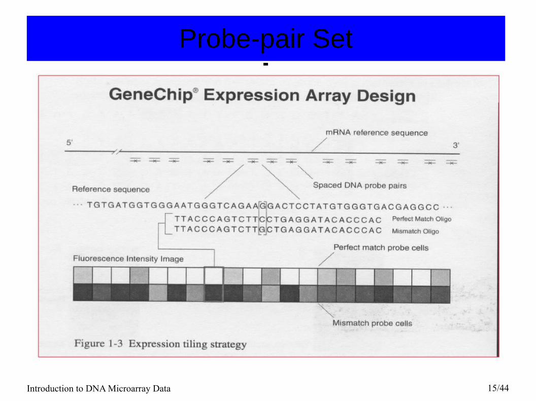
Oligonucleotide chips (Affymetrix)● Each gene or portion of a gene is represented by 16 to 20

oligonucleotides of 25 base-pairs.● Probe: an oligonucleotide of 25 base-pairs, i.e., a 25-mer.

– Perfect match (PM): A 25-mer complementary to a reference sequence of interest (e.g., part of a gene).

– Mismatch (MM): same as PM but with a single homomeric base change for the middle (13th) base (transversion purine <-> pyrimidine, G <->C, A <->T) .

● Probe-pair: a (PM,MM) pair. ● The purpose of the MM probe design is to measure non-

specific binding and background noise.● Affy ID: an identifier for a probe-pair set.


Probe-pair Set


Part II

Pre-processing an affymetrix data related to prostate cancer with Bioconductor tools

Preliminary:

Install bioconductor and packages:> source("http://bioconductor.org/biocLite.R")

> biocLite ("affy") ## install affy package

> biocLite ("oligo") ## install oligo package

7 November 2014Introduction to DNA Microarray Data 17/44

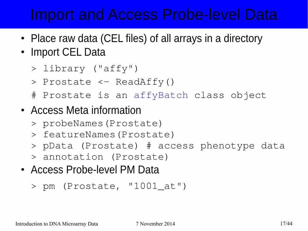
Import and Access Probe-level Data● Place raw data (CEL files) of all arrays in a directory● Import CEL Data> library ("affy")

> Prostate <- ReadAffy()

# Prostate is an affyBatch class object

● Access Meta information> probeNames(Prostate)> featureNames(Prostate) > pData (Prostate) # access phenotype data> annotation (Prostate)

● Access Probe-level PM Data> pm (Prostate, "1001_at")


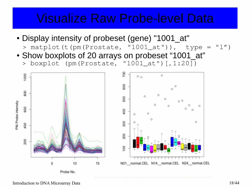
Visualize Raw Probe-level Data● Display intensity of probeset (gene) "1001_at" > matplot(t(pm(Prostate, "1001_at")), type = "l”)● Show boxplots of 20 arrays on probeset “1001_at”> boxplot (pm(Prostate, "1001_at")[,1:20])


Visualize Raw Probe-level DataDraw smoothed histograms of all probes of 50 arrays> hist (Prostate[,1:50], col = 1:50)


A Generic Error Model

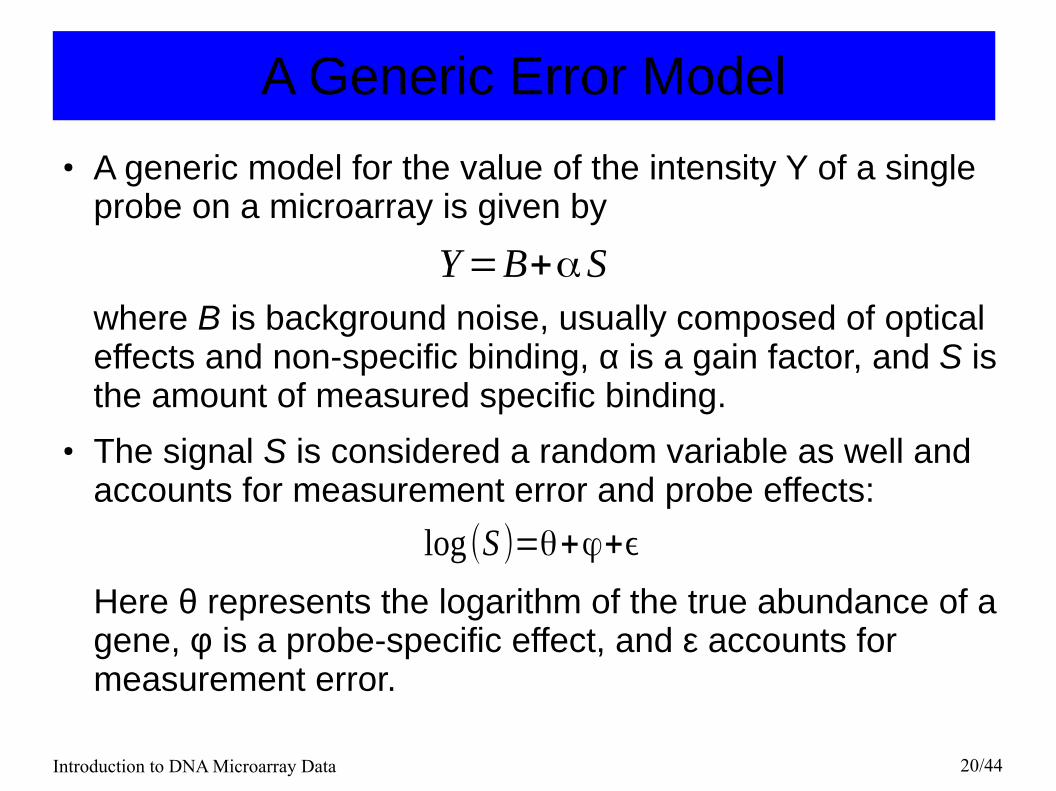
● A generic model for the value of the intensity Y of a single probe on a microarray is given by

where B is background noise, usually composed of optical effects and non-specific binding, α is a gain factor, and S is the amount of measured specific binding.

● The signal S is considered a random variable as well and accounts for measurement error and probe effects:

Here θ represents the logarithm of the true abundance of a gene, φ is a probe-specific effect, and ε accounts for measurement error.

Y=B+αS

log(S )=θ+ϕ+ϵ


Background Correction

Many background correction methods have been proposed in the microarray literature. Two examples:● MAS 5.0: The chip is divided into a grid of k (default k =

16) rectangular regions. For each region, the lowest 2% of probe intensities are used to compute a background value for that grid.

● RMA convolution: The observed PM probes are modelled as the sum of a Gaussian noise component, B, with mean μ and variance σ2 and an exponential signal component, S. Based on this model, adjust Y with:


Background Correction

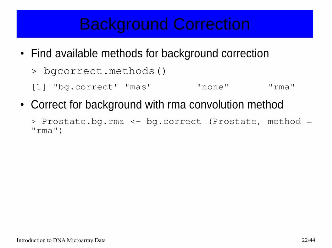
● Find available methods for background correction> bgcorrect.methods()

[1] "bg.correct" "mas" "none" "rma"

● Correct for background with rma convolution method> Prostate.bg.rma <- bg.correct (Prostate, method = "rma")


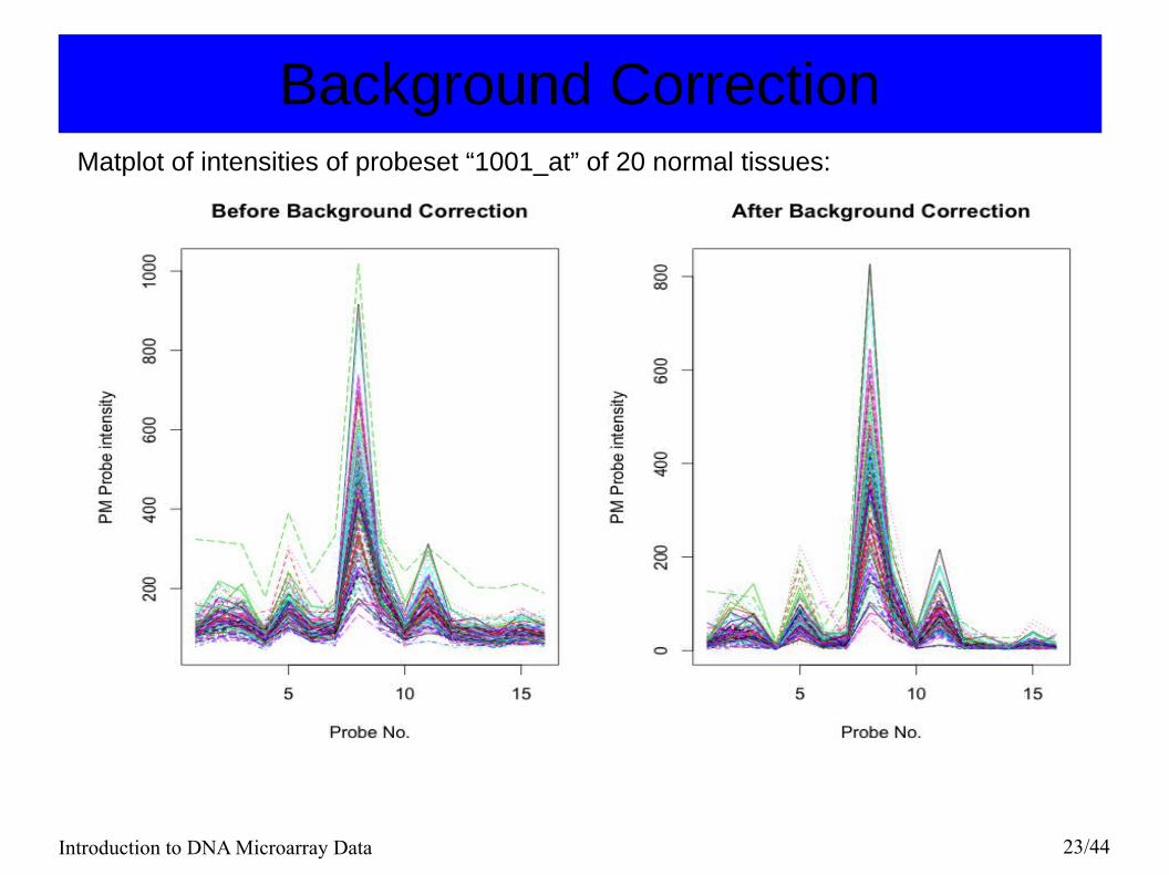
Background CorrectionMatplot of intensities of probeset “1001_at” of 20 normal tissues:


Background Correctionboxplot of intensities of probeset “1001_at” on 20 normal tissues:


Background CorrectionSmoothed histogram of all probe intensities of 50 arrays (tissues)


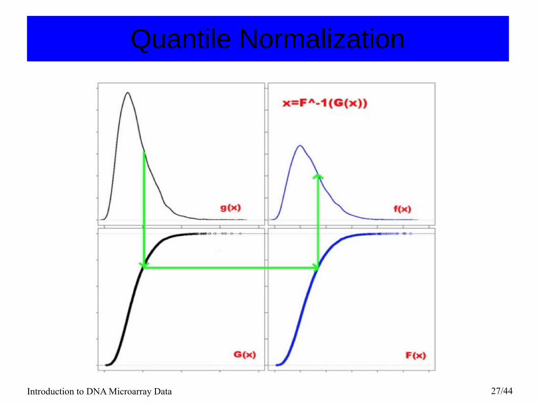
Normalization

Normalization refers to the task of manipulating data to make measurements from different arrays comparable. One characterization is that the gain factor α varies for different arrays. Many methods are proposed to normalize microarray data. Two examples:● Scaling: A baseline array is chosen and all the other arrays are

scaled to have the same mean intensity as this array. ● Quantile normalization: Impose the same empirical distribution of

intensities to all arrays.Transform each value with

xi = F−1 [G(xi)],

where G is estimated by the empirical distribution of each array and F is the empirical distribution of the averaged sample quantiles.


Quantile Normalization


Normalization

● Check available methods for normalizing> normalize.methods (Prostate)[1] "constant" "contrasts" "invariantset" [4] "loess" "methods" "qspline" [7] "quantiles" "quantiles.robust" "vsn" [10] "quantiles.probeset" "scaling"

● Normalize with quantiles method> Prostate.norm.quantile <- normalize (Prostate.bg.rma, method = "quantiles")


NormalizationMatplot of intensities of probeset “1001_at” of 20 normal tissues:


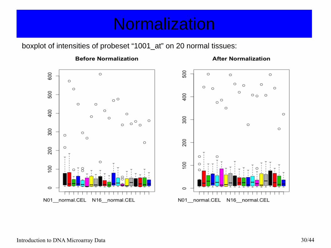
Normalizationboxplot of intensities of probeset “1001_at” on 20 normal tissues:


NormalizationSmoothed histogram of log intensities of all probes of 50 arrays (tissues)


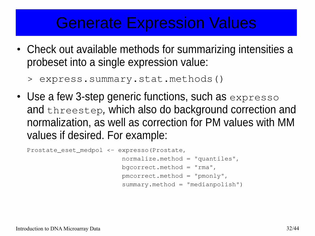
Generate Expression Values

● Check out available methods for summarizing intensities a probeset into a single expression value:> express.summary.stat.methods()

● Use a few 3-step generic functions, such as expresso and threestep, which also do background correction and normalization, as well as correction for PM values with MM values if desired. For example:Prostate_eset_medpol <- expresso(Prostate,

normalize.method = "quantiles",

bgcorrect.method = "rma",

pmcorrect.method = "pmonly",

summary.method = "medianpolish")


RMA Summary of Probe-level Intensities

● To obtain an expression measure, assume that for each probe set n, the background-adjusted, normalized, and log-transformed PM intensities, denoted with Yijn , follow a linear additive model:

Yijn =μin+αjn+εijn, i=1,...,I, j=1,...,J, n=1,...,N

with μi representing the log scale expression level for array i, αj a probe affinity effect, and εij representing an

independent identically distributed error term with mean 0.

● The estimate of μin gives the expression measures for probe set n on array i.


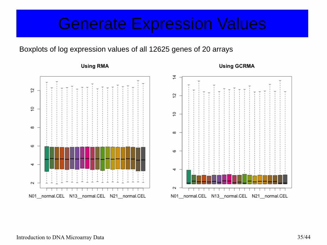
● There are also specialized functions that do all of the three steps, such as rma and gcrma. In rma function, RMA is used for background correction, quantile is used for normalization, and a robust multi-array method is used to summarize intensities of probesets.

– Using rma > Prostate_eset_rma <- rma (Prostate)

– Using gcrma> Prostate_eset_gcrma <- gcrma (Prostate)

● The results, such as Prostate_eset_rma, are an ExpressionSet object.

Generate Expression Values


Generate Expression ValuesBoxplots of log expression values of all 12625 genes of 20 arrays


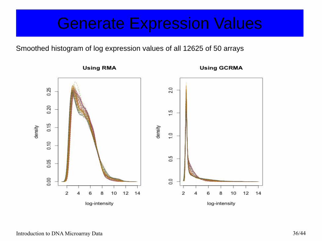
Generate Expression ValuesSmoothed histogram of log expression values of all 12625 of 50 arrays


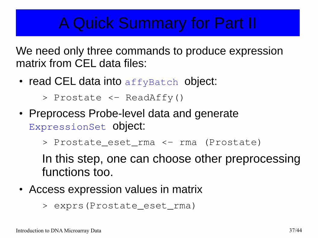
A Quick Summary for Part II

We need only three commands to produce expression matrix from CEL data files:● read CEL data into affyBatch object:

> Prostate <- ReadAffy()

● Preprocess Probe-level data and generate ExpressionSet object:

> Prostate_eset_rma <- rma (Prostate)

In this step, one can choose other preprocessing functions too.

● Access expression values in matrix> exprs(Prostate_eset_rma)


Part III

A Simple Example of Using Expression Data:

Finding differential genes related to a phenotype variable using univariate screening


Generate Top Genes Table

● Specify phenotype and design data> cancer <- c(rep (1, 50), rep (2, 52))

● Fit linear model for each gene as a response> fit_rma <- lmFit (Prostate_eset_rma, cancer)

● Compute moderated t-statistics and others by empirical Bayes moderation of the standard errors.> efit_rma <- eBayes (fit)

● Extract a table of the top-ranked genes> topTable_rma <- topTable (efit_rma, number = 20)

● Find a list of top genes (Probe ID)> topgenes_rma <- rownames (topTable_rma)


Generate Top Genes Table

A snapshot of top genes table:> head (topTable_rma)

logFC AveExpr t P.Value adj.P.Val B

41468_at 4.356643 6.920753 40.79516 5.549054e-67 7.005680e-63 142.5652

37639_at 5.087711 8.324154 39.22109 2.864858e-65 1.260118e-61 138.6458

37366_at 4.175774 6.743498 39.20376 2.994341e-65 1.260118e-61 138.6019

41706_at 3.774081 6.132773 38.32262 2.896583e-64 9.142341e-61 136.3449

36491_at 3.503627 5.665337 37.30346 4.232732e-63 1.068765e-59 133.6760

1740_g_at 3.799499 6.088183 36.83541 1.481559e-62 3.117447e-59 132.4287


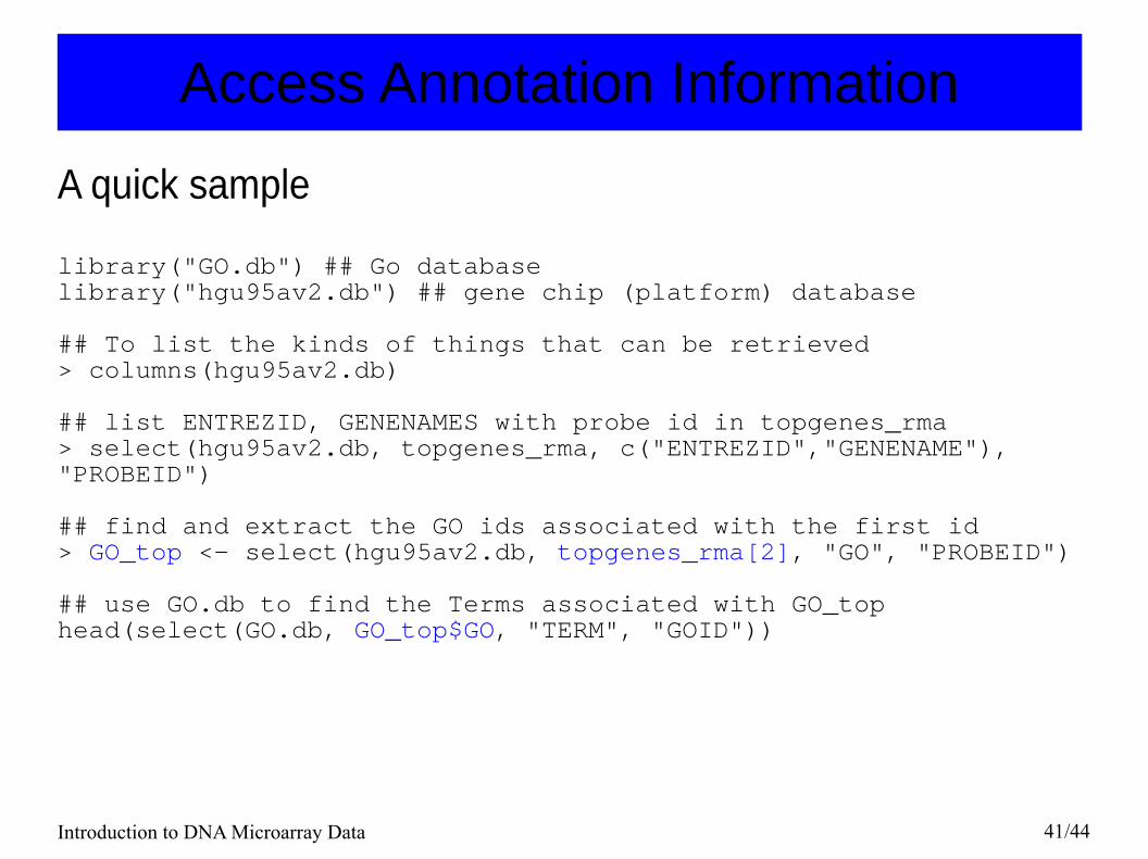
Access Annotation Information

A quick sample

library("GO.db") ## Go databaselibrary("hgu95av2.db") ## gene chip (platform) database

## To list the kinds of things that can be retrieved> columns(hgu95av2.db)

## list ENTREZID, GENENAMES with probe id in topgenes_rma> select(hgu95av2.db, topgenes_rma, c("ENTREZID","GENENAME"), "PROBEID")

## find and extract the GO ids associated with the first id> GO_top <- select(hgu95av2.db, topgenes_rma[2], "GO", "PROBEID")

## use GO.db to find the Terms associated with GO_tophead(select(GO.db, GO_top$GO, "TERM", "GOID"))


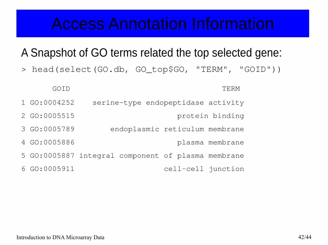
Access Annotation Information

A Snapshot of GO terms related the top selected gene:> head(select(GO.db, GO_top$GO, "TERM", "GOID"))

GOID TERM1 GO:0004252 serine-type endopeptidase activity

2 GO:0005515 protein binding

3 GO:0005789 endoplasmic reticulum membrane

4 GO:0005886 plasma membrane

5 GO:0005887 integral component of plasma membrane

6 GO:0005911 cell-cell junction


Conclusions and Discussions

● Today, it is very easy to generate and analyze micorarray expression matrix with bioconductor tools

● Microarray data have many limitations. The actual mRNA signals are contaminated by various noise, including background noise, varying gaining factor, and cross-hybridization noise. In addition, multiple probe sets represent the same gene.

● RNA-Seq is a powerful technology that is predicted to replace microarrays for transcriptome profiling. RNA-Seq avoids technical issues in microarray studies related to probe performance such as cross-hybridization. However, the cost of RNA-seq is still too high. Also, the tools for RNA-Seq data analysis are far from mature.


References

● Gentleman, Robert, Vincent J. Carey, Wolfgang Huber, Rafael A. Irizarry, and Sandrine Dudoit. Bioinformatics and Computational Biology Solutions Using R and Bioconductor. Springer, 2005.

The book is free and comprehensive. ● http://www.bioconductor.org. The website contains a large

archive of software documentations, workshop slides, and workflow examples for different tasks.

http://www.bioconductor.org/

introduction to dna microarray data - mathematics and...

Documents