introduction to econometric production analysis with r - itslearning
TRANSCRIPT

Introduction to Econometric
Production Analysis with R
(Draft Version)
Arne Henningsen
Department of Food and Resource Economics
University of Copenhagen
October 28, 2014

Foreword
This is an incomplete collection of my lecture notes for various courses in the field of econometric
production analysis. These lecture notes are still incomplete and may contain many typos, errors,
and inconsistencies. Please report any problems to [email protected]. I am grateful
to my former students who helped me to improve my teaching and these notes through their
questions, suggestions, and comments. Finally, I thank the R community for providing so many
excellent tools for econometric production analysis.
October 28, 2014
Arne Henningsen
2

Contents
1 Introduction 10
1.1 Objectives of the course and the lecture notes . . . . . . . . . . . . . . . . . . . . . 10
1.2 An extremely short introduction to R . . . . . . . . . . . . . . . . . . . . . . . . . . 10
1.2.1 Some commands for simple calculations . . . . . . . . . . . . . . . . . . . . 10
1.2.2 Creating objects and assigning values . . . . . . . . . . . . . . . . . . . . . 12
1.2.3 Vectors . . . . . . . . . . . . . . . . . . . . . . . . . . . . . . . . . . . . . . 13
1.2.4 Simple functions . . . . . . . . . . . . . . . . . . . . . . . . . . . . . . . . . 14
1.2.5 Comparing values and boolean values . . . . . . . . . . . . . . . . . . . . . 15
1.2.6 Data sets (“data frames”) . . . . . . . . . . . . . . . . . . . . . . . . . . . . 16
1.2.7 Functions . . . . . . . . . . . . . . . . . . . . . . . . . . . . . . . . . . . . . 18
1.2.8 Simple graphics . . . . . . . . . . . . . . . . . . . . . . . . . . . . . . . . . . 18
1.2.9 Other useful comands . . . . . . . . . . . . . . . . . . . . . . . . . . . . . . 19
1.2.10 Extension packages . . . . . . . . . . . . . . . . . . . . . . . . . . . . . . . . 19
1.2.11 Reading data into R . . . . . . . . . . . . . . . . . . . . . . . . . . . . . . . 20
1.2.12 Linear regression . . . . . . . . . . . . . . . . . . . . . . . . . . . . . . . . . 20
1.3 Data sets . . . . . . . . . . . . . . . . . . . . . . . . . . . . . . . . . . . . . . . . . 26
1.3.1 French apple producers . . . . . . . . . . . . . . . . . . . . . . . . . . . . . 26
1.3.1.1 Description of the data set . . . . . . . . . . . . . . . . . . . . . . 26
1.3.1.2 Abbreviating name of data set . . . . . . . . . . . . . . . . . . . . 27
1.3.1.3 Calculation of input quantities . . . . . . . . . . . . . . . . . . . . 27
1.3.1.4 Calculation of total costs and variable costs . . . . . . . . . . . . . 27
1.3.1.5 Calculation of profit and gross margin . . . . . . . . . . . . . . . . 28
1.3.2 Rice producers on the Philippines . . . . . . . . . . . . . . . . . . . . . . . 28
1.3.2.1 Description of the data set . . . . . . . . . . . . . . . . . . . . . . 28
1.3.2.2 Mean-scaling Quantities . . . . . . . . . . . . . . . . . . . . . . . . 29
1.3.2.3 Logarithmic Mean-scaled Quantities . . . . . . . . . . . . . . . . . 29
1.3.2.4 Mean-adjusting the Time Trend . . . . . . . . . . . . . . . . . . . 30
1.3.2.5 Specifying Panel Structure . . . . . . . . . . . . . . . . . . . . . . 30
1.4 Mathematical and statistical methods . . . . . . . . . . . . . . . . . . . . . . . . . 30
1.4.1 Aggregating quantities . . . . . . . . . . . . . . . . . . . . . . . . . . . . . . 30
1.4.2 Quasiconcavity . . . . . . . . . . . . . . . . . . . . . . . . . . . . . . . . . . 32
1.4.3 Delta method . . . . . . . . . . . . . . . . . . . . . . . . . . . . . . . . . . . 32
3

Contents
2 Primal Approach: Production Function 34
2.1 Theory . . . . . . . . . . . . . . . . . . . . . . . . . . . . . . . . . . . . . . . . . . . 34
2.1.1 Production function . . . . . . . . . . . . . . . . . . . . . . . . . . . . . . . 34
2.1.2 Average Products . . . . . . . . . . . . . . . . . . . . . . . . . . . . . . . . 34
2.1.3 Total Factor Productivity . . . . . . . . . . . . . . . . . . . . . . . . . . . . 34
2.1.4 Marginal Products . . . . . . . . . . . . . . . . . . . . . . . . . . . . . . . . 35
2.1.5 Output elasticities . . . . . . . . . . . . . . . . . . . . . . . . . . . . . . . . 35
2.1.6 Elasticity of scale . . . . . . . . . . . . . . . . . . . . . . . . . . . . . . . . . 35
2.1.7 Marginal rates of technical substitution . . . . . . . . . . . . . . . . . . . . 36
2.1.8 Relative marginal rates of technical substitution . . . . . . . . . . . . . . . 36
2.1.9 Elasticities of substitution . . . . . . . . . . . . . . . . . . . . . . . . . . . . 36
2.1.9.1 Direct Elasticities of Substitution . . . . . . . . . . . . . . . . . . 36
2.1.9.2 Allen Elasticities of Substitution . . . . . . . . . . . . . . . . . . . 37
2.1.9.3 Morishima Elasticities of Substitution . . . . . . . . . . . . . . . . 38
2.1.10 Profit Maximization . . . . . . . . . . . . . . . . . . . . . . . . . . . . . . . 38
2.1.11 Cost Minimization . . . . . . . . . . . . . . . . . . . . . . . . . . . . . . . . 39
2.1.12 Derived Input Demand Functions and Output Supply Functions . . . . . . 40
2.1.12.1 Derived from profit maximization . . . . . . . . . . . . . . . . . . 40
2.1.12.2 Derived from cost minimization . . . . . . . . . . . . . . . . . . . 41
2.2 Productivity Measures . . . . . . . . . . . . . . . . . . . . . . . . . . . . . . . . . . 42
2.2.1 Average Products . . . . . . . . . . . . . . . . . . . . . . . . . . . . . . . . 42
2.2.2 Total Factor Productivity . . . . . . . . . . . . . . . . . . . . . . . . . . . . 44
2.3 Linear Production Function . . . . . . . . . . . . . . . . . . . . . . . . . . . . . . . 46
2.3.1 Specification . . . . . . . . . . . . . . . . . . . . . . . . . . . . . . . . . . . 46
2.3.2 Estimation . . . . . . . . . . . . . . . . . . . . . . . . . . . . . . . . . . . . 46
2.3.3 Properties . . . . . . . . . . . . . . . . . . . . . . . . . . . . . . . . . . . . . 46
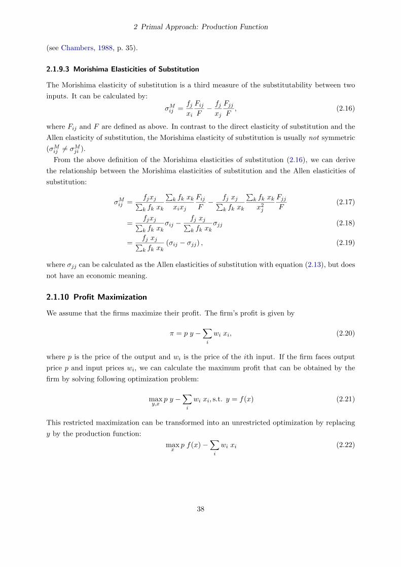
2.3.4 Predicted output quantities . . . . . . . . . . . . . . . . . . . . . . . . . . . 47
2.3.5 Marginal Products . . . . . . . . . . . . . . . . . . . . . . . . . . . . . . . . 48
2.3.6 Output Elasticities . . . . . . . . . . . . . . . . . . . . . . . . . . . . . . . . 48
2.3.7 Elasticity of Scale . . . . . . . . . . . . . . . . . . . . . . . . . . . . . . . . 51
2.3.8 Marginal rates of technical substitution . . . . . . . . . . . . . . . . . . . . 54
2.3.9 Relative marginal rates of technical substitution . . . . . . . . . . . . . . . 55
2.3.10 First-order conditions for profit maximisation . . . . . . . . . . . . . . . . . 55
2.3.11 First-order conditions for cost minimization . . . . . . . . . . . . . . . . . . 58
2.3.12 Derived Input Demand Functions and Output Supply Functions . . . . . . 60
2.4 Cobb-Douglas production function . . . . . . . . . . . . . . . . . . . . . . . . . . . 61
2.4.1 Specification . . . . . . . . . . . . . . . . . . . . . . . . . . . . . . . . . . . 61
2.4.2 Estimation . . . . . . . . . . . . . . . . . . . . . . . . . . . . . . . . . . . . 61
2.4.3 Properties . . . . . . . . . . . . . . . . . . . . . . . . . . . . . . . . . . . . . 62
4

Contents
2.4.4 Predicted output quantities . . . . . . . . . . . . . . . . . . . . . . . . . . . 62
2.4.5 Output elasticities . . . . . . . . . . . . . . . . . . . . . . . . . . . . . . . . 63
2.4.6 Marginal products . . . . . . . . . . . . . . . . . . . . . . . . . . . . . . . . 63
2.4.7 Elasticity of Scale . . . . . . . . . . . . . . . . . . . . . . . . . . . . . . . . 64
2.4.8 Marginal Rates of Technical Substitution . . . . . . . . . . . . . . . . . . . 66
2.4.9 Relative Marginal Rates of Technical Substitution . . . . . . . . . . . . . . 67
2.4.10 First and second partial derivatives . . . . . . . . . . . . . . . . . . . . . . . 68
2.4.11 Elasticities of substitution . . . . . . . . . . . . . . . . . . . . . . . . . . . . 70
2.4.11.1 Direct Elasticities of Substitution . . . . . . . . . . . . . . . . . . 70
2.4.11.2 Allen Elasticities of Substitution . . . . . . . . . . . . . . . . . . . 72
2.4.11.3 Morishima Elasticities of Substitution . . . . . . . . . . . . . . . . 73
2.4.12 Quasiconcavity . . . . . . . . . . . . . . . . . . . . . . . . . . . . . . . . . . 74
2.4.13 First-order conditions for profit maximisation . . . . . . . . . . . . . . . . . 75
2.4.14 First-order conditions for cost minimization . . . . . . . . . . . . . . . . . . 77
2.4.15 Derived Input Demand Functions and Output Supply Functions . . . . . . 79
2.4.16 Derived Input Demand Elasticities . . . . . . . . . . . . . . . . . . . . . . . 82
2.5 Quadratic Production Function . . . . . . . . . . . . . . . . . . . . . . . . . . . . . 84
2.5.1 Specification . . . . . . . . . . . . . . . . . . . . . . . . . . . . . . . . . . . 84
2.5.2 Estimation . . . . . . . . . . . . . . . . . . . . . . . . . . . . . . . . . . . . 85
2.5.3 Properties . . . . . . . . . . . . . . . . . . . . . . . . . . . . . . . . . . . . . 87
2.5.4 Predicted output quantities . . . . . . . . . . . . . . . . . . . . . . . . . . . 87
2.5.5 Marginal Products . . . . . . . . . . . . . . . . . . . . . . . . . . . . . . . . 88
2.5.6 Output Elasticities . . . . . . . . . . . . . . . . . . . . . . . . . . . . . . . . 90
2.5.7 Elasticity of Scale . . . . . . . . . . . . . . . . . . . . . . . . . . . . . . . . 90
2.5.8 Marginal Rates of Technical Substitution . . . . . . . . . . . . . . . . . . . 91
2.5.9 Relative Marginal Rates of Technical Substitution . . . . . . . . . . . . . . 93
2.5.10 Elasticities of Substitution . . . . . . . . . . . . . . . . . . . . . . . . . . . . 95
2.5.11 Quasiconcavity . . . . . . . . . . . . . . . . . . . . . . . . . . . . . . . . . . 98
2.5.12 First-order conditions for profit maximisation . . . . . . . . . . . . . . . . . 98
2.5.13 First-order conditions for cost minimization . . . . . . . . . . . . . . . . . . 99
2.6 Translog Production Function . . . . . . . . . . . . . . . . . . . . . . . . . . . . . . 102
2.6.1 Specification . . . . . . . . . . . . . . . . . . . . . . . . . . . . . . . . . . . 102
2.6.2 Estimation . . . . . . . . . . . . . . . . . . . . . . . . . . . . . . . . . . . . 102
2.6.3 Properties . . . . . . . . . . . . . . . . . . . . . . . . . . . . . . . . . . . . . 104
2.6.4 Predicted Output Quantities . . . . . . . . . . . . . . . . . . . . . . . . . . 105
2.6.5 Output Elasticities . . . . . . . . . . . . . . . . . . . . . . . . . . . . . . . . 105
2.6.6 Marginal Products . . . . . . . . . . . . . . . . . . . . . . . . . . . . . . . . 107
2.6.7 Elasticity of Scale . . . . . . . . . . . . . . . . . . . . . . . . . . . . . . . . 108
2.6.8 Marginal Rates of Technical Substitution . . . . . . . . . . . . . . . . . . . 109
5
Contents
2.6.9 Relative Marginal Rates of Technical Substitution . . . . . . . . . . . . . . 111
2.6.10 Second partial derivatives . . . . . . . . . . . . . . . . . . . . . . . . . . . . 113
2.6.11 Elasticities of Substitution . . . . . . . . . . . . . . . . . . . . . . . . . . . . 114
2.6.12 Quasiconcavity . . . . . . . . . . . . . . . . . . . . . . . . . . . . . . . . . . 117
2.6.13 First-order conditions for profit maximisation . . . . . . . . . . . . . . . . . 117
2.6.14 First-order conditions for cost minimization . . . . . . . . . . . . . . . . . . 119
2.6.15 Mean-scaled quantities . . . . . . . . . . . . . . . . . . . . . . . . . . . . . . 122
2.7 Evaluation of Different Functional Forms . . . . . . . . . . . . . . . . . . . . . . . 124
2.7.1 Goodness of Fit . . . . . . . . . . . . . . . . . . . . . . . . . . . . . . . . . . 124
2.7.2 Theoretical Consistency . . . . . . . . . . . . . . . . . . . . . . . . . . . . . 125
2.7.3 Plausible Estimates . . . . . . . . . . . . . . . . . . . . . . . . . . . . . . . 126
2.7.4 Summary . . . . . . . . . . . . . . . . . . . . . . . . . . . . . . . . . . . . . 127
2.8 Non-parametric production function . . . . . . . . . . . . . . . . . . . . . . . . . . 127
3 Dual Approach: Cost Functions 133
3.1 Theory . . . . . . . . . . . . . . . . . . . . . . . . . . . . . . . . . . . . . . . . . . . 133
3.1.1 Cost function . . . . . . . . . . . . . . . . . . . . . . . . . . . . . . . . . . . 133
3.1.2 Cost flexibility and elasticity of size . . . . . . . . . . . . . . . . . . . . . . 133
3.1.3 Short-Run Cost Functions . . . . . . . . . . . . . . . . . . . . . . . . . . . . 133
3.2 Cobb-Douglas Cost Function . . . . . . . . . . . . . . . . . . . . . . . . . . . . . . 134
3.2.1 Specification . . . . . . . . . . . . . . . . . . . . . . . . . . . . . . . . . . . 134
3.2.2 Estimation . . . . . . . . . . . . . . . . . . . . . . . . . . . . . . . . . . . . 134
3.2.3 Properties . . . . . . . . . . . . . . . . . . . . . . . . . . . . . . . . . . . . . 135
3.2.4 Estimation with linear homogeneity in input prices imposed . . . . . . . . . 136
3.2.5 Checking Concavity in Input Prices . . . . . . . . . . . . . . . . . . . . . . 138
3.2.6 Optimal Cost Shares . . . . . . . . . . . . . . . . . . . . . . . . . . . . . . . 143
3.2.7 Derived Input Demand Functions . . . . . . . . . . . . . . . . . . . . . . . . 144
3.2.8 Derived Input Demand Elasticities . . . . . . . . . . . . . . . . . . . . . . . 147
3.2.9 Cost flexibility and elasticity of size . . . . . . . . . . . . . . . . . . . . . . 149
3.2.10 Marginal Costs, Average Costs, and Total Costs . . . . . . . . . . . . . . . 149
3.3 Cobb-Douglas Short-Run Cost Function . . . . . . . . . . . . . . . . . . . . . . . . 152
3.3.1 Specification . . . . . . . . . . . . . . . . . . . . . . . . . . . . . . . . . . . 152
3.3.2 Estimation . . . . . . . . . . . . . . . . . . . . . . . . . . . . . . . . . . . . 153
3.3.3 Properties . . . . . . . . . . . . . . . . . . . . . . . . . . . . . . . . . . . . . 153
3.3.4 Estimation with linear homogeneity in input prices imposed . . . . . . . . . 154
3.4 Translog cost function . . . . . . . . . . . . . . . . . . . . . . . . . . . . . . . . . . 155
3.4.1 Specification . . . . . . . . . . . . . . . . . . . . . . . . . . . . . . . . . . . 155
3.4.2 Estimation . . . . . . . . . . . . . . . . . . . . . . . . . . . . . . . . . . . . 156
3.4.3 Linear homogeneity in input prices . . . . . . . . . . . . . . . . . . . . . . . 157
3.4.4 Estimation with linear homogeneity in input prices imposed . . . . . . . . . 159
6

Contents
3.4.5 Cost Flexibility and Elasticity of Size . . . . . . . . . . . . . . . . . . . . . 163
3.4.6 Marginal Costs and Average Costs . . . . . . . . . . . . . . . . . . . . . . . 164
3.4.7 Derived Input Demand Functions . . . . . . . . . . . . . . . . . . . . . . . . 168
3.4.8 Derived input demand elasticities . . . . . . . . . . . . . . . . . . . . . . . . 170
3.4.9 Theoretical consistency . . . . . . . . . . . . . . . . . . . . . . . . . . . . . 173
4 Dual Approach: Profit Function 177
4.1 Theory . . . . . . . . . . . . . . . . . . . . . . . . . . . . . . . . . . . . . . . . . . . 177
4.1.1 Profit functions . . . . . . . . . . . . . . . . . . . . . . . . . . . . . . . . . . 177
4.1.2 Short-run profit functions . . . . . . . . . . . . . . . . . . . . . . . . . . . . 177
4.2 Graphical illustration of profit and gross margin . . . . . . . . . . . . . . . . . . . 177
4.3 Cobb-Douglas Profit Function . . . . . . . . . . . . . . . . . . . . . . . . . . . . . . 179
4.3.1 Specification . . . . . . . . . . . . . . . . . . . . . . . . . . . . . . . . . . . 179
4.3.2 Estimation . . . . . . . . . . . . . . . . . . . . . . . . . . . . . . . . . . . . 180
4.3.3 Properties . . . . . . . . . . . . . . . . . . . . . . . . . . . . . . . . . . . . . 180
4.3.4 Estimation with linear homogeneity in all prices imposed . . . . . . . . . . 181
4.3.5 Checking Convexity in all prices . . . . . . . . . . . . . . . . . . . . . . . . 183
4.3.6 Predicted profit . . . . . . . . . . . . . . . . . . . . . . . . . . . . . . . . . . 188
4.3.7 Optimal Profit Shares . . . . . . . . . . . . . . . . . . . . . . . . . . . . . . 189
4.3.8 Derived Output Supply Input Demand Functions . . . . . . . . . . . . . . . 191
4.3.9 Derived Output Supply and Input Demand Elasticities . . . . . . . . . . . . 191
4.4 Cobb-Douglas Short-Run Profit Function . . . . . . . . . . . . . . . . . . . . . . . 193
4.4.1 Specification . . . . . . . . . . . . . . . . . . . . . . . . . . . . . . . . . . . 193
4.4.2 Estimation . . . . . . . . . . . . . . . . . . . . . . . . . . . . . . . . . . . . 194
4.4.3 Properties . . . . . . . . . . . . . . . . . . . . . . . . . . . . . . . . . . . . . 194
4.4.4 Estimation with linear homogeneity in all prices imposed . . . . . . . . . . 195
4.4.5 Returns to scale . . . . . . . . . . . . . . . . . . . . . . . . . . . . . . . . . 196
4.4.6 Shadow prices of quasi-fixed inputs . . . . . . . . . . . . . . . . . . . . . . . 196
5 Stochastic Frontier Analysis 198
5.1 Theory . . . . . . . . . . . . . . . . . . . . . . . . . . . . . . . . . . . . . . . . . . . 198
5.1.1 Different Efficiency Measures . . . . . . . . . . . . . . . . . . . . . . . . . . 198
5.1.1.1 Output-Oriented Technical Efficiency with One Output . . . . . . 198
5.1.1.2 Input-Oriented Technical Efficiency with One Input . . . . . . . . 198
5.1.1.3 Output-Oriented Technical Efficiency with Two or More Outputs 198
5.1.1.4 Input-Oriented Technical Efficiency with Two or More Inputs . . 199
5.1.1.5 Output-Oriented Allocative Efficiency and Revenue Efficiency . . 199
5.1.1.6 Input-Oriented Allocative Efficiency and Cost Efficiency . . . . . . 200
5.1.1.7 Profit Efficiency . . . . . . . . . . . . . . . . . . . . . . . . . . . . 200
5.1.1.8 Scale efficiency . . . . . . . . . . . . . . . . . . . . . . . . . . . . . 201
7

Contents
5.2 Stochastic Production Frontiers . . . . . . . . . . . . . . . . . . . . . . . . . . . . . 201
5.2.1 Specification . . . . . . . . . . . . . . . . . . . . . . . . . . . . . . . . . . . 201
5.2.1.1 Marginal products and output elasticities in SFA models . . . . . 203
5.2.2 Skewness of residuals from OLS estimations . . . . . . . . . . . . . . . . . . 203
5.2.3 Cobb-Douglas Stochastic Production Frontier . . . . . . . . . . . . . . . . . 204
5.2.4 Translog Production Frontier . . . . . . . . . . . . . . . . . . . . . . . . . . 209
5.2.5 Translog Production Frontier with Mean-Scaled Variables . . . . . . . . . . 211
5.3 Stochastic Cost Frontiers . . . . . . . . . . . . . . . . . . . . . . . . . . . . . . . . 213
5.3.1 Specification . . . . . . . . . . . . . . . . . . . . . . . . . . . . . . . . . . . 213
5.3.2 Skewness of residuals from OLS estimations . . . . . . . . . . . . . . . . . . 214
5.3.3 Estimation of a Cobb-Douglas stochastic cost frontier . . . . . . . . . . . . 215
5.4 Analyzing the Effects of z Variables . . . . . . . . . . . . . . . . . . . . . . . . . . 217
5.4.1 Production Functions with z Variables . . . . . . . . . . . . . . . . . . . . . 218
5.4.2 Production Frontiers with z Variables . . . . . . . . . . . . . . . . . . . . . 219
5.4.3 Efficiency Effects Production Frontiers . . . . . . . . . . . . . . . . . . . . . 222
6 Data Envelopment Analysis (DEA) 227
6.1 Preparations . . . . . . . . . . . . . . . . . . . . . . . . . . . . . . . . . . . . . . . 227
6.2 DEA with input-oriented efficiencies . . . . . . . . . . . . . . . . . . . . . . . . . . 227
6.3 DEA with output-oriented efficiencies . . . . . . . . . . . . . . . . . . . . . . . . . 230
6.4 DEA with “super efficiencies” . . . . . . . . . . . . . . . . . . . . . . . . . . . . . . 230
6.5 DEA with graph hyperbolic efficiencies . . . . . . . . . . . . . . . . . . . . . . . . . 230
7 Panel Data and Technological Change 231
7.1 Average Production Functions with Technological Change . . . . . . . . . . . . . . 231
7.1.1 Cobb-Douglas Production Function with Technological Change . . . . . . . 231
7.1.1.1 Pooled estimation of the Cobb-Douglas Production Function with
Technological Change . . . . . . . . . . . . . . . . . . . . . . . . . 232
7.1.1.2 Panel data estimations of the Cobb-Douglas Production Function
with Technological Change . . . . . . . . . . . . . . . . . . . . . . 233
7.1.2 Translog Production Function with Constant and Neutral Technological
Change . . . . . . . . . . . . . . . . . . . . . . . . . . . . . . . . . . . . . . 237
7.1.2.1 Pooled estimation of the Translog Production Function with Con-
stant and Neutral Technological Change . . . . . . . . . . . . . . . 238
7.1.2.2 Panel-data estimations of the Translog Production Function with
Constant and Neutral Technological Change . . . . . . . . . . . . 239
7.1.3 Translog Production Function with Non-Constant and Non-Neutral Tech-
nological Change . . . . . . . . . . . . . . . . . . . . . . . . . . . . . . . . . 245
7.1.3.1 Pooled Estimation of a Translog Production Function with Non-
Constant and Non-Neutral Technological Change . . . . . . . . . . 245
8

Contents
7.1.3.2 Panel-data estimations of a Translog Production Function with
Non-Constant and Non-Neutral Technological Change . . . . . . . 251
7.2 Frontier Production Functions with Technological Change . . . . . . . . . . . . . . 257
7.2.1 Cobb-Douglas Production Frontier with Technological Change . . . . . . . 257
7.2.1.1 Time-invariant Individual Efficiencies . . . . . . . . . . . . . . . . 257
7.2.1.2 Time-variant Individual Efficiencies . . . . . . . . . . . . . . . . . 260
7.2.1.3 Observation-specific efficiencies . . . . . . . . . . . . . . . . . . . . 265
7.2.2 Translog Production Frontier with Constant and Neutral Technological
Change . . . . . . . . . . . . . . . . . . . . . . . . . . . . . . . . . . . . . . 267
7.2.2.1 Observation-Specific Efficiencies . . . . . . . . . . . . . . . . . . . 267
7.2.3 Translog Production Frontier with Non-Constant and Non-Neutral Tech-
nological Change . . . . . . . . . . . . . . . . . . . . . . . . . . . . . . . . . 270
7.2.3.1 Observation-Specific Efficiencies . . . . . . . . . . . . . . . . . . . 270
7.2.4 Decomposition of Productivity Growth . . . . . . . . . . . . . . . . . . . . . 273
7.3 Analysing Productivity Growths with Data Envelopment Analysis (DEA) . . . . . 274
9

1 Introduction
1.1 Objectives of the course and the lecture notes
Knowledge about production technologies and producer behavior is important for politicians,
business organizations, government administrations, financial institutions, the EU, and other na-
tional and international organizations who desire to know how contemplated policies and market
conditions can affect production, prices, income, and resource utilization in agriculture as well as
in other industries. The same knowledge is relevant in consultancy of single firms who also want
to compare themselves with other firms and their technology with the best practice technology.
The participants of my courses in the field of econometric production analysis will obtain
relevant theoretical knowledge and practical skills so that they can contribute to the knowledge
about production technologies and producer behavior. After completing my courses in the field
of econometric production analysis, the students should be able to:
� use econometric production analysis and efficiency analysis to analyze various real-world
questions,
� interpret the results of econometric production analyses and efficiency analyses,
� choose a relevant approach for econometric production and efficiency analysis, and
� critically evaluate the appropriateness of a specific econometric production analysis or effi-
ciency analysis for analyzing a specific real-world question.
These lecture notes focus on practical applications of econometrics and microeconomic pro-
duction theory. Hence, they complement textbooks in microeconomic production theory (rather
than substituting them).
1.2 An extremely short introduction to R
Many tutorials for learning R are freely available on-line, e.g. the official “Introduction to R”
(http://cran.r-project.org/doc/manuals/r-release/R-intro.pdf) or the many tutorials
listed in the category“Contributed Documentation”(http://cran.r-project.org/other-docs.
html). Furthermore, many good books are available, e.g. “A Beginner’s Guide to R” (Zuur, Ieno,
and Meesters, 2009), “R Cookbook” (Teetor, 2011), or “Applied Econometrics with R” (Kleiber
and Zeileis, 2008).
10

1 Introduction
1.2.1 Some commands for simple calculations
R is my favourite “pocket calculator”. . .
> 2 + 3
[1] 5
> 2 - 3
[1] -1
> 2 * 3
[1] 6
> 2 / 3
[1] 0.6666667
> 2^3
[1] 8
R uses the standard order of evaluation (as in mathematics). One can use parenthesis (round
brackets) to change the order of evaluation.
> 2 + 3 * 4^2
[1] 50
> 2 + ( 3 * ( 4^2 ) )
[1] 50
> ( ( 2 + 3 ) * 4 )^2
[1] 400
In R, the hash symbol (#) can be used to add comments to the code, because the hash symbol
and all following characters in the same line are ignored by R.
> sqrt(2) # square root
[1] 1.414214
> 2^(1/2) # the same
11

1 Introduction
[1] 1.414214
> 2^0.5 # also the same
[1] 1.414214
> log(3) # natural logarithm
[1] 1.098612
> exp(3) # exponential function
[1] 20.08554
The commands can span multiple lines. They are executed as soon as the command can be
considered as complete.
> 2 +
+ 3
[1] 5
> ( 2
+ +
+ 3 )
[1] 5
1.2.2 Creating objects and assigning values
> a <- 2
> a
[1] 2
> b <- 3
> b
[1] 3
> a * b
[1] 6
Initially, the arrow symbol (<-, consistent of a “smaller than” sign and a dash) was used to assign
values to objects. However, in recent versions of R, also the equality sign (=) can be used for this.
12

1 Introduction
> a = 4
> a
[1] 4
> b = 5
> b
[1] 5
> a * b
[1] 20
In these lecture notes, I stick to the traditional assignment operator, i.e. the arrow symbol (<-).
Please note that R is case-sensitive, i.e. R distinguishes between upper-case and lower-case
letters. Therefore, the following commands return error messages:
> A # NOT the same as "a"
> B # NOT the same as "b"
> Log(3) # NOT the same as "log(3)"
> LOG(3) # NOT the same as "log(3)"
1.2.3 Vectors
> v <- 1:4 # create a vector with 4 elements: 1, 2, 3, and 4
> v
[1] 1 2 3 4
> 2 + v # adding 2 to each element
[1] 3 4 5 6
> 2 * v # multiplying each element by 2
[1] 2 4 6 8
> log( v ) # the natural logarithm of each element
[1] 0.0000000 0.6931472 1.0986123 1.3862944
> w <- c( 2, 4, 8, 16 ) # concatenate 4 numbers to a vector
> w
13

1 Introduction
[1] 2 4 8 16
> v + w # element-wise addition
[1] 3 6 11 20
> v * w # element-wise multiplication
[1] 2 8 24 64
> v %*% w # scalar product (inner product)
[,1]
[1,] 98
> w[2] # select the second element
[1] 4
> w[c(1,3)] # select the first and the third element
[1] 2 8
> w[2:4] # select the second, third, and fourth element
[1] 4 8 16
> w[-2] # select all but the second element
[1] 2 8 16
> length( w )
[1] 4
1.2.4 Simple functions
> sum( w )
[1] 30
> mean( w )
[1] 7.5
> median( w )
14

1 Introduction
[1] 6
> min( w )
[1] 2
> max( w )
[1] 16
> which.min( w )
[1] 1
> which.max( w )
[1] 4
1.2.5 Comparing values and boolean values
> a == 2
[1] FALSE
> a != 2
[1] TRUE
> a > 4
[1] FALSE
> a >= 4
[1] TRUE
> w > 3
[1] FALSE TRUE TRUE TRUE
> w == 2^(1:4)
[1] TRUE TRUE TRUE TRUE
> all.equal( w, 2^(1:4) )
[1] TRUE
> w > 3 & w < 6 # ampersand = and
[1] FALSE TRUE FALSE FALSE
> w < 3 | w > 6 # vertical line = or
[1] TRUE FALSE TRUE TRUE
15

1 Introduction
1.2.6 Data sets (“data frames”)
The data set “women” is included in R.
> data( "women" ) # load the data set into the workspace
> women
height weight
1 58 115
2 59 117
3 60 120
4 61 123
5 62 126
6 63 129
7 64 132
8 65 135
9 66 139
10 67 142
11 68 146
12 69 150
13 70 154
14 71 159
15 72 164
> names( women ) # display the variable names
[1] "height" "weight"
> dim( women ) # dimension of the data set (rows and columns)
[1] 15 2
> nrow( women ) # number of rows (observations)
[1] 15
> ncol( women ) # number of columns (variables)
[1] 2
> women[[ "height" ]] # display the values of variable "height"
[1] 58 59 60 61 62 63 64 65 66 67 68 69 70 71 72
> women$height # short-cut for the previous command
16

1 Introduction
[1] 58 59 60 61 62 63 64 65 66 67 68 69 70 71 72
> women$height[ 3 ] # height of the third observation
[1] 60
> women[ 3, "height" ] # the same
[1] 60
> women[ 3, 1 ] # also the same
[1] 60
> women[ 1:3, 1 ] # height of the first three observations
[1] 58 59 60
> women[ 1:3, ] # all variables of the first three observations
height weight
1 58 115
2 59 117
3 60 120
> women$cmHeight <- 2.54 * women$height # new variable: height in cm
> women$kgWeight <- women$weight / 2.205 # new variable: weight in kg
> women$bmi <- women$kgWeight / ( women$cmHeight / 100 )^2 # new variable: BMI
> women
height weight cmHeight kgWeight bmi
1 58 115 147.32 52.15420 24.03067
2 59 117 149.86 53.06122 23.62685
3 60 120 152.40 54.42177 23.43164
4 61 123 154.94 55.78231 23.23643
5 62 126 157.48 57.14286 23.04152
6 63 129 160.02 58.50340 22.84718
7 64 132 162.56 59.86395 22.65364
8 65 135 165.10 61.22449 22.46110
9 66 139 167.64 63.03855 22.43112
10 67 142 170.18 64.39909 22.23631
11 68 146 172.72 66.21315 22.19520
12 69 150 175.26 68.02721 22.14711
13 70 154 177.80 69.84127 22.09269
14 71 159 180.34 72.10884 22.17198
15 72 164 182.88 74.37642 22.23836
17

1 Introduction
1.2.7 Functions
In order to execute a function in R, the function name has to be followed by a pair of parenthesis
(round brackets). The documentation of a function (if available) can be obtained by, e.g., typing
at the R prompt a question mark followed by the name of the function.
> ?log
One can read in the documentation of the function log, e.g., that this function has a second
optional argument base, which can be used to specify the base of the logarithm. By default, the
base is equal to the Euler number (e, exp(1)). A different base can be chosen by adding a second
argument, either with or without specifying the name of the argument.
> log( 100, base = 10 )
[1] 2
> log( 100, 10 )
[1] 2
1.2.8 Simple graphics
Histograms can be created with the command hist. The optional argument breaks can be used
to specify the approximate number of cells:
> hist( women$bmi )
> hist( women$bmi, breaks = 10 )
women$bmi
Fre
quen
cy
22.0 22.5 23.0 23.5 24.0 24.5
02
46
8
women$bmi
Fre
quen
cy
22.0 22.5 23.0 23.5 24.0
01
23
4
Figure 1.1: Histogram of BMIs
The resulting histogram is shown in figure 1.1.
Scatter plots can be created with the command plot:
> plot( women$height, women$weight )
The resulting scatter plot is shown in figure 1.2.
18

1 Introduction
●●
●
●
●
●
●
●
●
●
●
●
●
●
●
58 60 62 64 66 68 70 72
120
130
140
150
160
women$height
wom
en$w
eigh
t
Figure 1.2: Scatter plot of heights and weights
1.2.9 Other useful comands
> class( a )
[1] "numeric"
> class( women )
[1] "data.frame"
> class( women$height )
[1] "numeric"
> ls() # list all objects in the workspace
[1] "a" "b" "v" "w" "women"
> rm(w) # remove an object
> ls()
[1] "a" "b" "v" "women"
1.2.10 Extension packages
Currently (June 12, 2013, 2pm GMT), 4611 extension packages for R are available on CRAN
(Comprehensive R Archive Network, http://cran.r-project.org). When an extension package
is installed, it can be loaded with the command library. The following command loads the R
package foreign that includes function for reading data in various formats.
> library( "foreign" )
19

1 Introduction
Please note that you should cite scientific software packages in your publications if you used them
for obtaining your results (as any other scientific works). You can use the command citation
to find out how an R package should be cited, e.g.:
> citation( "frontier" )
To cite package 'frontier' in publications use:
Tim Coelli and Arne Henningsen (2013). frontier: Stochastic Frontier
Analysis. R package version 1.1-0.
http://CRAN.R-Project.org/package=frontier.
A BibTeX entry for LaTeX users is
@Manual{,
title = {frontier: Stochastic Frontier Analysis},
author = {Tim Coelli and Arne Henningsen},
year = {2013},
note = {R package version 1.1-0},
url = {http://CRAN.R-Project.org/package=frontier},
}
1.2.11 Reading data into R
R can read and import data from many different file formats. This is described in the official
R manual “R Data Import/Export” (http://cran.r-project.org/doc/manuals/r-release/
R-data.pdf). I usually read my data into R from files in CSV (comma separated values) format.
This can be done by the function read.csv. The command read.csv2 can read files in the
“European CSV format” (values separated by semicolons, comma as decimal separator). The
functions read.dta, read.spss, and read.xport (all in package foreign) can read STATA binary
files, SPSS data files, and SAS “XPORT” files, respectively. Functions for reading MS-Excel files
are available, e.g., in the packages XLConnect and xlsx.
1.2.12 Linear regression
The command for estimating linear models in R is lm. The first argument of the command lm
specifies the model that should be estimated. This must be a formula object that consists of the
name of the dependent variable, followed by a tilde (~) and the name of the explanatory variable.
Argument data can be used to specify the data set:
> olsWeight <- lm( weight ~ height, data = women )
> olsWeight
20

1 Introduction
Call:
lm(formula = weight ~ height, data = women)
Coefficients:
(Intercept) height
-87.52 3.45
The summary method can be used to display summary statistics of the regression:
> summary( olsWeight )
Call:
lm(formula = weight ~ height, data = women)
Residuals:
Min 1Q Median 3Q Max
-1.7333 -1.1333 -0.3833 0.7417 3.1167
Coefficients:
Estimate Std. Error t value Pr(>|t|)
(Intercept) -87.51667 5.93694 -14.74 1.71e-09 ***
height 3.45000 0.09114 37.85 1.09e-14 ***
---
Signif. codes: 0 ‘***’ 0.001 ‘**’ 0.01 ‘*’ 0.05 ‘.’ 0.1 ‘ ’ 1
Residual standard error: 1.525 on 13 degrees of freedom
Multiple R-squared: 0.991, Adjusted R-squared: 0.9903
F-statistic: 1433 on 1 and 13 DF, p-value: 1.091e-14
The command abline can be used to add a linear (regression) line to a (scatter) plot:
> plot( women$height, women$weight )
> abline( olsWeight )
The resulting plot is shown in figure 1.3. This figure indicates that the relationship between
the height and the corresponding average weights of the women is slightly nonlinear. Therefore,
we add the squared height as additional explanatory regressor. When specifying more than one
explanatory variable, the names of the explanatory variables must be separated by plus signs (+):
> women$heightSquared <- women$height^2
> olsWeight2 <- lm( weight ~ height + heightSquared, data = women )
> summary( olsWeight2 )
21

1 Introduction
●●
●
●
●
●
●
●
●
●
●
●
●
●
●
58 60 62 64 66 68 70 72
120
130
140
150
160
women$height
wom
en$w
eigh
t
Figure 1.3: Scatter plot of heights and weights with estimated regression line
Call:
lm(formula = weight ~ height + heightSquared, data = women)
Residuals:
Min 1Q Median 3Q Max
-0.50941 -0.29611 -0.00941 0.28615 0.59706
Coefficients:
Estimate Std. Error t value Pr(>|t|)
(Intercept) 261.87818 25.19677 10.393 2.36e-07 ***
height -7.34832 0.77769 -9.449 6.58e-07 ***
heightSquared 0.08306 0.00598 13.891 9.32e-09 ***
---
Signif. codes: 0 ‘***’ 0.001 ‘**’ 0.01 ‘*’ 0.05 ‘.’ 0.1 ‘ ’ 1
Residual standard error: 0.3841 on 12 degrees of freedom
Multiple R-squared: 0.9995, Adjusted R-squared: 0.9994
F-statistic: 1.139e+04 on 2 and 12 DF, p-value: < 2.2e-16
One can use the functiom I() to calculate explanatory variables directly in the formula:
> olsWeight3 <- lm( weight ~ height + I(height^2), data = women )
> summary( olsWeight3 )
Call:
lm(formula = weight ~ height + I(height^2), data = women)
22

1 Introduction
Residuals:
Min 1Q Median 3Q Max
-0.50941 -0.29611 -0.00941 0.28615 0.59706
Coefficients:
Estimate Std. Error t value Pr(>|t|)
(Intercept) 261.87818 25.19677 10.393 2.36e-07 ***
height -7.34832 0.77769 -9.449 6.58e-07 ***
I(height^2) 0.08306 0.00598 13.891 9.32e-09 ***
---
Signif. codes: 0 ‘***’ 0.001 ‘**’ 0.01 ‘*’ 0.05 ‘.’ 0.1 ‘ ’ 1
Residual standard error: 0.3841 on 12 degrees of freedom
Multiple R-squared: 0.9995, Adjusted R-squared: 0.9994
F-statistic: 1.139e+04 on 2 and 12 DF, p-value: < 2.2e-16
The coef method for lm objects can be used to extract the vector of the estimated coefficients:
> coef( olsWeight2 )
(Intercept) height heightSquared
261.87818358 -7.34831933 0.08306399
When the coef method is applied to the object returned by the summary method for lm
objects, the matrix of the estimated coefficients, their standard errors, their t-values, and their
P -values is returned:
> coef( summary( olsWeight2 ) )
Estimate Std. Error t value Pr(>|t|)
(Intercept) 261.87818358 25.196770820 10.393323 2.356879e-07
height -7.34831933 0.777692280 -9.448878 6.584476e-07
heightSquared 0.08306399 0.005979642 13.891131 9.322439e-09
The variance covariance matrix of the estimated coefficients can be obtained by the vcov
method:
> vcov( olsWeight2 )
(Intercept) height heightSquared
(Intercept) 634.8772597 -19.586524729 1.504022e-01
height -19.5865247 0.604805283 -4.648296e-03
heightSquared 0.1504022 -0.004648296 3.575612e-05
23

1 Introduction
The residuals method for lm objects can be used to obtain the residuals:
> residuals( olsWeight2 )
1 2 3 4 5 6
-0.102941176 -0.473109244 -0.009405301 0.288170653 0.419618617 0.384938591
7 8 9 10 11 12
0.184130575 -0.182805430 0.284130575 -0.415061409 -0.280381383 -0.311829347
13 14 15
-0.509405301 0.126890756 0.597058824
The fitted method for lm objects can be used to obtain the fitted values:
> fitted( olsWeight2 )
1 2 3 4 5 6 7 8
115.1029 117.4731 120.0094 122.7118 125.5804 128.6151 131.8159 135.1828
9 10 11 12 13 14 15
138.7159 142.4151 146.2804 150.3118 154.5094 158.8731 163.4029
We can evaluate the “fit” of the model by plotting the fitted values against the observed values
of the dependent variable and adding a 45-degree line:
> plot( women$weight, fitted( olsWeight2 ) )
> abline(0,1)
●●
●
●
●
●
●
●
●
●
●
●
●
●
●
120 130 140 150 160
120
130
140
150
160
women$weight
fitte
d(ol
sWei
ght2
)
Figure 1.4: Observed and fitted values of the dependent variable
The resulting scatter plot is shown in figure 1.4.
The plot method for lm objects can be used to generate diagnostic plots
> plot( olsWeight2 )
The resulting diagnostic plots are shown in figure 1.5.
24

1 Introduction
120 130 140 150 160
−0.
6−
0.2
0.2
0.6
Fitted values
Res
idua
ls
●
●
●
●
●●
●
●
●
●
●●
●
●
●
Residuals vs Fitted
15
132
●
●
●
●
●●
●
●
●
●
●●
●
●
●
−1 0 1
−1
01
2
Theoretical Quantiles
Sta
ndar
dize
d re
sidu
als
Normal Q−Q
15
13 2
120 130 140 150 160
0.0
0.5
1.0
1.5
Fitted values
Sta
ndar
dize
d re
sidu
als
●
●
●
●
●●
● ●
●
●
●●
●
●
●
Scale−Location15
132
0.0 0.1 0.2 0.3 0.4
−1
01
2
Leverage
Sta
ndar
dize
d re
sidu
als
●
●
●
●
●●
●
●
●
●
●●
●
●
●
Cook's distance
Residuals vs Leverage
15
213
Figure 1.5: Diagnostic plots
25

1 Introduction
1.3 Data sets
In my courses in the field of econometric production analysis, I usually use two data sets: one
cross-sectional data set of French apple producers and a panel data set of rice producers on the
Philippines.
1.3.1 French apple producers
1.3.1.1 Description of the data set
In this course, we will predominantly use a cross-sectional production data set of 140 French
apple producers from the year 1986. These data are extracted from a panel data set that has
been used in an article published by Ivaldi et al. (1996) in the Journal of Applied Econometrics.
The full panel data set is available in the journal’s data archive: http://www.econ.queensu.
ca/jae/1996-v11.6/ivaldi-ladoux-ossard-simioni/.1
The cross-sectional data set that we will predominantly use in the course is available in the R
package micEcon. It has the name appleProdFr86 and can be loaded by the command:
> data( "appleProdFr86", package = "micEcon" )
The names of the variables in the data set can be obtained by the command names:
> names( appleProdFr86 )
[1] "vCap" "vLab" "vMat" "qApples" "qOtherOut" "qOut"
[7] "pCap" "pLab" "pMat" "pOut" "adv"
The data set includes following variables:2
vCap costs of capital (including land)
vLab costs of labor (including remuneration of unpaid family labor)
vMat costs of intermediate materials (e.g. seedlings, fertilizer, pesticides, fuel)
qOut quantity index of all outputs (apples and other outputs)
pCap price index of capital goods
pLab price index of labor
pMat price index of materials
pOut price index of the aggregate output∗
adv use of advisory service∗
Please note that variables indicated by ∗ are not in the original data set but are artificially
generated in order to be able to conduct some further analyses with this data set. Variable names
starting with v indicate volumes (values), variable names starting with q indicate quantities, and
variable names starting with p indicate prices.
1 In order to focus on the microeconomic analysis rather than on econometric issues in panel data analysis, weonly use a single year from this panel data set.
2 This information is also available in the documentation of this data set, which can be obtained by the command:help( "appleProdFr86", package = "micEcon" ).
26

1 Introduction
1.3.1.2 Abbreviating name of data set
In order to avoid too much typing, give the data set a much shorter name (dat) by creating a
copy of the data set and removing the original data set:
> dat <- appleProdFr86
> rm( appleProdFr86 )
1.3.1.3 Calculation of input quantities
Our data set does not contain input quantities but prices and costs (volumes) of the inputs.
As we will need to know input quantities for many of our analyses, we calculate input quantity
indices based on following identity:
vi = xi · wi, (1.1)
where wi is the price, xi is the quantity and vi is the volume of the ith input. In R, we can
calculate the input quantities with the following commands:
> dat$qCap <- dat$vCap / dat$pCap
> dat$qLab <- dat$vLab / dat$pLab
> dat$qMat <- dat$vMat / dat$pMat
1.3.1.4 Calculation of total costs and variable costs
Total costs are defined as:
c =N∑i=1
wi xi, (1.2)
where N denotes the number of inputs. We can calculate the apple producers’ total costs by
following command:
> dat$cost <- with( dat, vCap + vLab + vMat )
Alternatively, we can calculate the costs by summing up the products of the quantities and the
corresponding prices over all inputs:
> all.equal( dat$cost, with( dat, pCap * qCap + pLab * qLab + pMat * qMat ) )
[1] TRUE
Variable costs are defined as:
cv =∑i∈N1
wi xi, (1.3)
where N1 is a vector of the indices of the variable inputs. If capital is a quasi-fixed input and
labor and materials are variable inputs, the apple producers’ variable costs can be calculated by
following command:
> dat$vCost <- with( dat, vLab + vMat )
27
1 Introduction
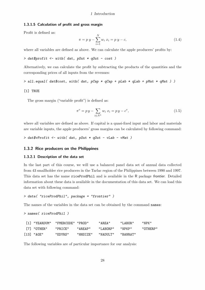
1.3.1.5 Calculation of profit and gross margin
Profit is defined as:
π = p y −N∑i=1
wi xi = p y − c, (1.4)
where all variables are defined as above. We can calculate the apple producers’ profits by:
> dat$profit <- with( dat, pOut * qOut - cost )
Alternatively, we can calculate the profit by subtracting the products of the quantities and the
corresponding prices of all inputs from the revenues:
> all.equal( dat$cost, with( dat, pCap * qCap + pLab * qLab + pMat * qMat ) )
[1] TRUE
The gross margin (“variable profit”) is defined as:
πv = p y −∑i∈N1
wi xi = p y − cv, (1.5)
where all variables are defined as above. If capital is a quasi-fixed input and labor and materials
are variable inputs, the apple producers’ gross margins can be calculated by following command:
> dat$vProfit <- with( dat, pOut * qOut - vLab - vMat )
1.3.2 Rice producers on the Philippines
1.3.2.1 Description of the data set
In the last part of this course, we will use a balanced panel data set of annual data collected
from 43 smallholder rice producers in the Tarlac region of the Philippines between 1990 and 1997.
This data set has the name riceProdPhil and is available in the R package frontier. Detailed
information about these data is available in the documentation of this data set. We can load this
data set with following command:
> data( "riceProdPhil", package = "frontier" )
The names of the variables in the data set can be obtained by the command names:
> names( riceProdPhil )
[1] "YEARDUM" "FMERCODE" "PROD" "AREA" "LABOR" "NPK"
[7] "OTHER" "PRICE" "AREAP" "LABORP" "NPKP" "OTHERP"
[13] "AGE" "EDYRS" "HHSIZE" "NADULT" "BANRAT"
The following variables are of particular importance for our analysis:
28
1 Introduction
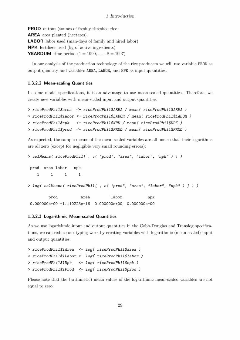
PROD output (tonnes of freshly threshed rice)
AREA area planted (hectares).
LABOR labor used (man-days of family and hired labor)
NPK fertilizer used (kg of active ingredients)
YEARDUM time period (1 = 1990, . . . , 8 = 1997)
In our analysis of the production technology of the rice producers we will use variable PROD as
output quantity and variables AREA, LABOR, and NPK as input quantities.
1.3.2.2 Mean-scaling Quantities
In some model specifications, it is an advantage to use mean-scaled quantities. Therefore, we
create new variables with mean-scaled input and output quantities:
> riceProdPhil$area <- riceProdPhil$AREA / mean( riceProdPhil$AREA )
> riceProdPhil$labor <- riceProdPhil$LABOR / mean( riceProdPhil$LABOR )
> riceProdPhil$npk <- riceProdPhil$NPK / mean( riceProdPhil$NPK )
> riceProdPhil$prod <- riceProdPhil$PROD / mean( riceProdPhil$PROD )
As expected, the sample means of the mean-scaled variables are all one so that their logarithms
are all zero (except for negligible very small rounding errors):
> colMeans( riceProdPhil[ , c( "prod", "area", "labor", "npk" ) ] )
prod area labor npk
1 1 1 1
> log( colMeans( riceProdPhil[ , c( "prod", "area", "labor", "npk" ) ] ) )
prod area labor npk
0.000000e+00 -1.110223e-16 0.000000e+00 0.000000e+00
1.3.2.3 Logarithmic Mean-scaled Quantities
As we use logarithmic input and output quantities in the Cobb-Douglas and Translog specifica-
tions, we can reduce our typing work by creating variables with logarithmic (mean-scaled) input
and output quantities:
> riceProdPhil$lArea <- log( riceProdPhil$area )
> riceProdPhil$lLabor <- log( riceProdPhil$labor )
> riceProdPhil$lNpk <- log( riceProdPhil$npk )
> riceProdPhil$lProd <- log( riceProdPhil$prod )
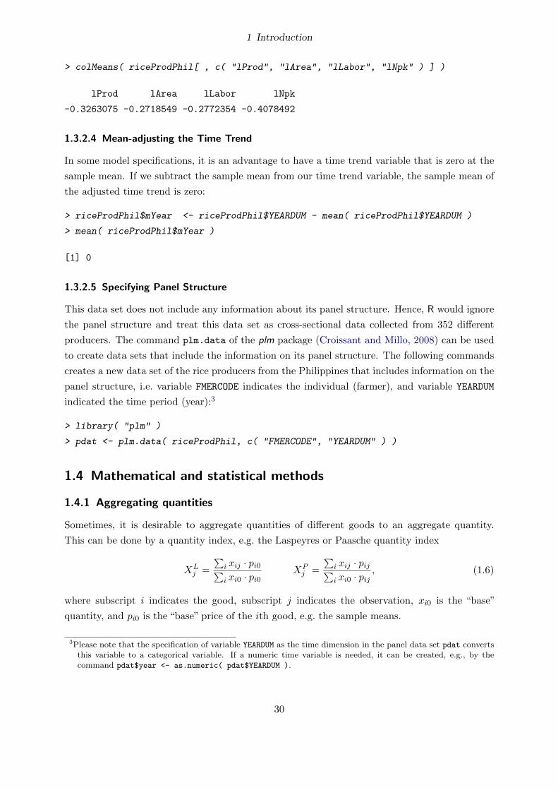
Please note that the (arithmetic) mean values of the logarithmic mean-scaled variables are not
equal to zero:
29
1 Introduction
> colMeans( riceProdPhil[ , c( "lProd", "lArea", "lLabor", "lNpk" ) ] )
lProd lArea lLabor lNpk
-0.3263075 -0.2718549 -0.2772354 -0.4078492
1.3.2.4 Mean-adjusting the Time Trend
In some model specifications, it is an advantage to have a time trend variable that is zero at the
sample mean. If we subtract the sample mean from our time trend variable, the sample mean of
the adjusted time trend is zero:
> riceProdPhil$mYear <- riceProdPhil$YEARDUM - mean( riceProdPhil$YEARDUM )
> mean( riceProdPhil$mYear )
[1] 0
1.3.2.5 Specifying Panel Structure
This data set does not include any information about its panel structure. Hence, R would ignore
the panel structure and treat this data set as cross-sectional data collected from 352 different
producers. The command plm.data of the plm package (Croissant and Millo, 2008) can be used
to create data sets that include the information on its panel structure. The following commands
creates a new data set of the rice producers from the Philippines that includes information on the
panel structure, i.e. variable FMERCODE indicates the individual (farmer), and variable YEARDUM
indicated the time period (year):3
> library( "plm" )
> pdat <- plm.data( riceProdPhil, c( "FMERCODE", "YEARDUM" ) )
1.4 Mathematical and statistical methods
1.4.1 Aggregating quantities
Sometimes, it is desirable to aggregate quantities of different goods to an aggregate quantity.
This can be done by a quantity index, e.g. the Laspeyres or Paasche quantity index
XLj =
∑i xij · pi0∑i xi0 · pi0
XPj =
∑i xij · pij∑i xi0 · pij
, (1.6)
where subscript i indicates the good, subscript j indicates the observation, xi0 is the “base”
quantity, and pi0 is the “base” price of the ith good, e.g. the sample means.
3Please note that the specification of variable YEARDUM as the time dimension in the panel data set pdat convertsthis variable to a categorical variable. If a numeric time variable is needed, it can be created, e.g., by thecommand pdat$year <- as.numeric( pdat$YEARDUM ).
30

1 Introduction
The Paasche and Laspeyres quantity indices of all three inputs in the data set of French apple
producers can be calculated by:
> dat$XP <- with( dat,
+ ( vCap + vLab + vMat ) /
+ ( mean( qCap ) * pCap + mean( qLab ) * pLab + mean( qMat ) * pMat ) )
> dat$XL <- with( dat,
+ ( qCap * mean( pCap ) + qLab * mean( pLab ) + qMat * mean( pMat ) ) /
+ ( mean( qCap ) * mean( pCap ) + mean( qLab ) * mean( pLab ) +
+ mean( qMat ) * mean( pMat ) ) )
In many cases, the choice of the formula for calculating quantity indices does not have a major
influence on the result. We demonstrate this with two scatter plots, where we set argument log
of the second plot command to the character string "xy" so that both axes are measured in
logarithmic terms and the dots (firms) are more equally spread:
> plot( dat$XP, dat$XL )
> plot( dat$XP, dat$XL, log = "xy" )
●●
●●●
●
●●
●●●
●
●
●●●
●
●
●●
●
●
●●●●
●
●
●●
●●●
●●
●●
●●
●●●●●●
●
●●●
●●●●●
●●●●●
●
●●
●
●●
●●
●
●
●
●●●●
●
●
●
●●●
●
●
●
●
●
●
●●●
●
●●
●
●
●
●
●●
●
●
●
●
●●
●●
●
●
●
●
●●
●●●
●
●●●
●
●●●
●●
●●
●
●
●
●
●
●
●
●●
●
●
●
●
1 2 3 4 5
12
34
5
XP
XL ●
●
●
● ●
●
●●
● ●
●
●
●
●●
●
●
●
●
●
●
●
●●
●●
●
●
●
●
●
● ●
●●
●
●
●
●
●●●
●
●●
●
●
●●
●●●●
●
●●●
●
●
●
●
●
●
●
●
●●
●
●
●
●●●
●
●
●
●
●●
●
●
●
●
●
●
●
●
●●
●
●●
●
●
●
●
●
●
●
●
●
●
●●
●
●
●
●
●
●
●●
●●
●
●
●
●●
●
●
●●
●●
●
●
●
●
●
●
●
●
●
●
●
●
●
●
●
0.5 1.0 2.0 5.0
0.5
1.0
2.0
5.0
XP
XL
Figure 1.6: Comparison of Paasche and Laspeyres quantity indices
The resulting scatter plots are shown in figure 1.6.
As a compromise, one can use the Fisher quantity index, which is the geometric mean of the
Paasche quantity index and the Laspeyres quantity index:
> dat$X <- sqrt( dat$XP * dat$XL )
We can can also use function quantityIndex from the micEcon package to calculate the quan-
tity index:
> library( "micEcon" )
> dat$XP2 <- quantityIndex( c( "pCap", "pLab", "pMat" ),
31

1 Introduction
+ c( "qCap", "qLab", "qMat" ), data = dat, method = "Paasche" )
> all.equal( dat$XP, dat$XP2, check.attributes = FALSE )
[1] TRUE
> dat$XL2 <- quantityIndex( c( "pCap", "pLab", "pMat" ),
+ c( "qCap", "qLab", "qMat" ), data = dat, method = "Laspeyres" )
> all.equal( dat$XL, dat$XL2, check.attributes = FALSE )
[1] TRUE
> dat$X2 <- quantityIndex( c( "pCap", "pLab", "pMat" ),
+ c( "qCap", "qLab", "qMat" ), data = dat, method = "Fisher" )
> all.equal( dat$X, dat$X2, check.attributes = FALSE )
[1] TRUE
1.4.2 Quasiconcavity
A function f(x) : RN → R is quasiconcave if its level plots (isoquants) are convex. This is the
case if
f(θxl + (1− θ)xu) ≥ min(f(xl), f(xu)) (1.7)
for any combination of xl, xu, and θ with 0 ≤ θ ≤ 1 (Chambers, 1988, p. 311).
If f(x) is a continuous and twice-continuously differentiable function, a necessary condition for
quasiconcavity is |B1| ≤ 0, |B2| ≥ 0, |B3| ≤ 0, . . . , (−1)N |BN | ≥ 0, where |Bi| is the ith principal
minor of the bordered Hessian
B =
0 f1 f2 . . . fN
f1 f11 f12 . . . f1N
f2 f12 f22 . . . f2N...
......
. . ....
fN f1N f2N . . . fNN
, (1.8)
fi denotes the partial derivative of f(x) with respect to xi, fij denotes the second partial derivative
of f(x) with respect to xi and xj , |B1| is the determinant of the upper left 2×2 sub-matrix of B,
|B2| is the determinant of the upper left 3× 3 sub-matrix of B, . . . , and |BN | is the determinant
of B (Chambers, 1988, p. 312; Chiang, 1984, p. 393f).
1.4.3 Delta method
If we have estimated a parameter vector β and its variance covariance matrix V ar(β) and we
calculate a vector of measures (e.g. elasticities) based on the estimated parameters by z = g(β),
32

1 Introduction
we can calculate the approximate variance covariance matrix of z by:
V ar(z) ≈(∂g(β)∂β
)>V ar(β) ∂g(β)
∂β, (1.9)
where ∂g(β)/∂β is the Jacobian matrix of z = g(β) with respect to β and the superscript > is
the transpose operator.
33

2 Primal Approach: Production Function
2.1 Theory
2.1.1 Production function
The production function
y = f(x) (2.1)
indicates the maximum quantity of a single output (y) that can be obtained with a vector of
given input quantities (x). It is usually assumed that production functions fulfill some properties
(see Chambers, 1988, p. 9).
2.1.2 Average Products
Very simple measures to compare the (partial) productivities of different firms are the inputs’
average products. The average product of the ith input is defined as:
APi = f(x)xi
= y
xi(2.2)
The more output one firm produces per unit of input, the more productive is this firm and
the higher is the corresponding average product. If two firms use identical input quantities,
the firm with the larger output quantity is more productive (has a higher average product).
And if two firms produce the same output quantity, the firm with the smaller input quantity is
more productive (has a higher average product). However, if these two firms use different input
combinations, one firm could be more productive regarding the average product of one input,
while the other firm could be more productive regarding the average product of another input.
2.1.3 Total Factor Productivity
As average products measure just partial productivities, it is often desirable to calculate total
factor productivities (TFP):
TFP = y
X, (2.3)
where X is a quantity index of all inputs (see section 1.4.1).
34

2 Primal Approach: Production Function
2.1.4 Marginal Products
The marginal productivities of the inputs can be measured by their marginal products. The
marginal product of the ith input is defined as:
MPi = ∂f(x)∂xi
(2.4)
2.1.5 Output elasticities
The marginal productivities of the inputs can also be measured by their output elasticities. The
output elasticity of the ith input is defined as:
εi = ∂f(x)∂xi
xif(x) = MP
AP(2.5)
In contrast to the marginal products, the changes of the input and output quantities are measured
in relative terms so that output elasticities are independent of the units of measurement. Output
elasticities are sometimes also called partial output elasticities or partial production elasticities.
2.1.6 Elasticity of scale
The returns of scale of the technology can be measured by the elasticity of scale:
ε =∑i
εi (2.6)
If the technology has increasing returns to scale (ε > 1), total factor productivity increases
when all input quantities are proportionally increased, because the relative increase of the output
quantity y is larger than the relative increase of the aggregate input quantity X in equation (2.3).
If the technology has decreasing returns to scale (ε < 1), total factor productivity decreases when
all input quantities are proportionally increased, because the relative increase of the output
quantity y is less than the relative increase of the aggregate input quantity X. If the technology
has constant returns to scale (ε = 1), total factor productivity remains constant when all input
quantities change proportionally, because the relative change of the output quantity y is equal to
the relative change of the aggregate input quantity X.
If the elasticity of scale (monotonically) decreases with firm size, the firm has the most pro-
ductive scale size at the point, where the elasticity of scale is one.
35

2 Primal Approach: Production Function
2.1.7 Marginal rates of technical substitution
The marginal rate of technical substitution between input i and input j is (Chambers, 1988,
p. 29):
MRTSi,j = ∂xi∂xj
= −
∂y
∂xj∂y
∂xi
= −MPjMPi
(2.7)
2.1.8 Relative marginal rates of technical substitution
The relative marginal rate of technical substitution between input i and input j is:
RMRTSi,j = ∂xi∂xj
xjxi
= −
∂y
∂xj∂y
∂xi
xjyxiy
= −εjεi
(2.8)
2.1.9 Elasticities of substitution
The elasticity of substitution measures the substitutability between two inputs. It is defined as:
σij =d(xixj
)d(MPjMPi
) MPjMPixixj
=d(xixj
)d (−MRTSij)
−MRTSijxixj
=d(xixj
)d MRTSij
MRTSijxixj
(2.9)
Thus, if input i is substituted for input j so that the input ratio xi/xj increases by σij%, the
marginal rate of technical substitution between input i and input j will increase by 1%.
2.1.9.1 Direct Elasticities of Substitution
The direct elasticity of substitution can be calculated by:
σDij = fi xi + fj xjxi xj
FijF, (2.10)
where F is the determinant of the bordered Hessian matrix B with
B =
0 f1 f2 . . . fN
f1 f11 f12 . . . f1N
f2 f12 f22 . . . f2N...
......
. . ....
fN f1N f2N . . . fNN
, (2.11)
36

2 Primal Approach: Production Function
Fij is the co-factor of fij , i.e.1
Fij = (−1)i+j ·
∣∣∣∣∣∣∣∣∣∣∣∣∣∣∣∣∣∣∣∣∣∣∣
0 f1 f2 . . . fj−1 fj+1 . . . fN
f1 f11 f12 . . . f1,j−1 f1,j+1 . . . f1N
f2 f12 f22 . . . f2,j−1 f2,j+1 . . . f2N...
......
. . ....
.... . .
...
fi−1 f1,i−1 f2,i−1 . . . fi−1,j−1 fi−1,j+1 . . . fi−1,N
fi+1 f1,i+1 f2,i+1 . . . fi+1,j−1 fi+1,j+1 . . . fi+1,N...
......
. . ....
.... . .
...
fN f1N f2N . . . fj−1,N fj+1,N . . . fNN
∣∣∣∣∣∣∣∣∣∣∣∣∣∣∣∣∣∣∣∣∣∣∣
, (2.12)
fi is the partial derivative of the production function f with respect to the ith input quantity
(xi), and fij is the second partial derivative of the production function f with respect to the ith
and jth input quantity (xi, xj).
As the bordered Hessian matrix is symmetric, the co-factors are also symmetric (Fij = Fji) so
that also the direct elasticities of substitution are symmetric (σDij = σDji ).
2.1.9.2 Allen Elasticities of Substitution
The Allen elasticity of substitution is another measure of the substitutability between two inputs.
It can be calculated by:
σij =∑k fk xkxi xj
FijF, (2.13)
where Fij and F are defined as above.
As with the direct elasticities of substitution, also the Allen elasticities of substitution are
symmetric (σij = σji).
The Allen elasticities of substitution are related to the direct elasticities of substitution in the
following way:
σDij = fi xi + fj xj∑k fk xk
∑k fk xkxi xj
FijF
= fi xi + fj xj∑k fk xk
σij (2.14)
As the input quantities and the marginal products should always be positive, the direct elasticities
of substitution and the Allen elasticities of substitution always have the same sign and the direct
elasticities of substitution are always smaller than the Allen elasticities of substitution in absolute
terms, i.e. |σDij | ≤ |σij |.Following condition holds for Allen elasticities of substitution:
∑i
Kiσij = 0 with Ki = fi xi∑k fk xk
(2.15)
1 The exponent of (−1) usually is the sum of the number of the deleted row (i+ 1) and the number of the deletedcolumn (j + 1), i.e. i+ j + 2. In our case, we can simplify this to i+ j, because (−1)i+j+2 = (−1)i+j · (−1)2 =(−1)i+j .
37
2 Primal Approach: Production Function
(see Chambers, 1988, p. 35).
2.1.9.3 Morishima Elasticities of Substitution
The Morishima elasticity of substitution is a third measure of the substitutability between two
inputs. It can be calculated by:
σMij = fjxi
FijF− fjxj
FjjF, (2.16)
where Fij and F are defined as above. In contrast to the direct elasticity of substitution and the
Allen elasticity of substitution, the Morishima elasticity of substitution is usually not symmetric
(σMij 6= σMji ).
From the above definition of the Morishima elasticities of substitution (2.16), we can derive
the relationship between the Morishima elasticities of substitution and the Allen elasticities of
substitution:
σMij = fjxj∑k fk xk
∑k fk xkxixj
FijF− fj xj∑
k fk xk
∑k fk xkx2j
FjjF
(2.17)
= fjxj∑k fk xk
σij −fj xj∑k fk xk
σjj (2.18)
= fj xj∑k fk xk
(σij − σjj) , (2.19)
where σjj can be calculated as the Allen elasticities of substitution with equation (2.13), but does
not have an economic meaning.
2.1.10 Profit Maximization
We assume that the firms maximize their profit. The firm’s profit is given by
π = p y −∑i
wi xi, (2.20)
where p is the price of the output and wi is the price of the ith input. If the firm faces output
price p and input prices wi, we can calculate the maximum profit that can be obtained by the
firm by solving following optimization problem:
maxy,x
p y −∑i
wi xi, s.t. y = f(x) (2.21)
This restricted maximization can be transformed into an unrestricted optimization by replacing
y by the production function:
maxx
p f(x)−∑i
wi xi (2.22)
38

2 Primal Approach: Production Function
Hence, the first-order conditions are:
∂π
∂xi= p
∂f(x)∂xi
− wi = p MPi − wi = 0 (2.23)
so that we get
wi = p MPi = MV Pi (2.24)
where MV Pi = p (∂y/∂xi) is the marginal value product of the ith input.
2.1.11 Cost Minimization
Now, we assume that the firms take total output as given (e.g. because production is restricted
by a quota) and try to produce this output quantity with minimal costs. The total cost is given
by
c =∑i
wi xi, (2.25)
where wi is the price of the ith input.
If the firm faces input prices wi and wants to produce y units of output, the minimum costs
can be obtained by
min∑i
wi xi, s.t. y = f(x) (2.26)
This restricted minimization can be solved by using the Lagrangian approach:
L =∑i
wi xi + λ (y − f(x)) (2.27)
So that the first-order conditions are:
∂L∂xi
= wi − λ∂f(x)∂xi
= wi − λ MPi = 0 (2.28)
∂L∂λ
= y − f(x) = 0 (2.29)
From the first-order conditions (2.28), we get:
wi = λMPi (2.30)
andwiwj
= λMPiλMPj
= MPiMPj
= −MRTSji (2.31)
As profit maximization implies producing the optimal output quantity with minimum costs,
the first-order conditions for the optimal input combinations (2.31) can be obtained not only
39

2 Primal Approach: Production Function
from cost minimization but also from the first-order conditions for profit maximization (2.24):
wiwj
= MV PiMV Pj
= p MPip MPj
= MPiMPj
= −MRTSji (2.32)
2.1.12 Derived Input Demand Functions and Output Supply Functions
In this section, we will analyze how profit maximizing or cost minimizing firms react on changing
prices and on changing output quantities.
2.1.12.1 Derived from profit maximization
If we replace the marginal products in the first-order conditions for profit maximization (2.24)
by the equations for calculating these marginal products and then solve this system of equations
for the input quantities, we get the input demand functions:
xi = xi(p, w), (2.33)
where w = [wi] is the vector of all input prices. The input demand functions indicate the optimal
input quantities (xi) given the output price (p) and all input prices (w). We can obtain the
output supply function from the production function by replacing all input quantities by the
corresponding input demand functions:
y = f(x(p, w)) = y(p, w), (2.34)
where x(p, w) = [xi(p, w)] is the set of all input demand functions. The output supply function
indicates the optimal output quantity (y) given the output price (p) and all input prices (w).
Hence, the input demand and output supply functions can be used to analyze the effects of prices
on the (optimal) input use and output supply. In economics, the effects of price changes are
usually measured in terms of price elasticities. These price elasticities can measure the effects of
the input prices on the input quantities:
εij(p, w) = ∂xi(p, w)∂wj
wjxi(p, w) , (2.35)
the effects of the input prices on the output quantity (expected to be non-positive):
εyj(p, w) = ∂y(p, w)∂wj
wjy(p, w) , (2.36)
the effects of the output price on the input quantities (expected to be non-negative):
εip(p, w) = ∂xi(p, w)∂p
p
xi(p, w) , (2.37)
40

2 Primal Approach: Production Function
and the effect of the output price on the output quantity (expected to be non-negative):
εyp(p, w) = ∂y(p, w)∂p
p
y(p, w) . (2.38)
The effect of an input price on the optimal quantity of the same input is expected to be non-
positive (εii(p, w) ≤ 0). If the cross-price elasticities between two inputs i and j are positive
(εij(p, w) ≥ 0, εji(p, w) ≥ 0), they are considered as gross substitutes. If the cross-price elasticities
between two inputs i and j are negative (εij(p, w) ≤ 0, εji(p, w) ≤ 0), they are considered as gross
complements.
2.1.12.2 Derived from cost minimization
If we replace the marginal products in the first-order conditions for cost minimization (2.30) by
the equations for calculating these marginal products and the solve this system of equations for
the input quantities, we get the conditional input demand functions:
xi = xi(w, y) (2.39)
These input demand functions are called “conditional,” because they indicate the optimal input
quantities (xi) given all input prices (w) and conditional on the fixed output quantity (y). The
conditional input demand functions can be used to analyze the effects of input prices on the
(optimal) input use if the output quantity is given. The effects of price changes on the optimal
input quantities can be measured by conditional price elasticities:
εij(w, y) = ∂xi(w, y)∂wj
wjxi(w, y) (2.40)
The effect of the output quantity on the optimal input quantities can also be measured in terms
of elasticities (expected to be positive):
εiy(w, y) = ∂xi(w, y)∂y
y
xi(w, y) . (2.41)
The conditional effect of an input price on the optimal quantity of the same input is expected
to be non-positive (εii(w, y) ≤ 0). If the conditional cross-price elasticities between two inputs i
and j are positive (εij(w, y) ≥ 0, εji(w, y) ≥ 0), they are considered as net substitutes. If
the conditional cross-price elasticities between two inputs i and j are negative (εij(w, y) ≤ 0,
εji(w, y) ≤ 0), they are considered as net complements.
41

2 Primal Approach: Production Function
2.2 Productivity Measures
2.2.1 Average Products
We calculate the average products of the three inputs for each firm in the data set by equation 2.2:
> dat$apCap <- dat$qOut / dat$qCap
> dat$apLab <- dat$qOut / dat$qLab
> dat$apMat <- dat$qOut / dat$qMat
We can visualize these average products with histograms that can be created with the command
hist.
> hist( dat$apCap )
> hist( dat$apLab )
> hist( dat$apMat )
apCap
Fre
quen
cy
0 50 100 150
010
2030
4050
60
apLab
Fre
quen
cy
0 5 10 15 20 25
05
1015
20
apMat
Fre
quen
cy
0 50 150 250 350
010
2030
4050
Figure 2.1: Average products
The resulting graphs are shown in figure 2.1. These graphs show that average products (partial
productivities) vary considerably between firms. Most firms in our data set produce on average
between 0 and 40 units of output per unit of capital, between 2 and 16 units of output per unit
of labor, and between 0 and 100 units of output per unit of materials. Looking at each average
product separately, There are usually many firms with medium to low productivity and only a
few firms with high productivity.
The relationships between the average products can be visualized by scatter plots:
> plot( dat$apCap, dat$apLab )
> plot( dat$apCap, dat$apMat )
> plot( dat$apLab, dat$apMat )
The resulting graphs are shown in figure 2.2. They show that the average products of the three
inputs are positively correlated.
42

2 Primal Approach: Production Function
●●
●
●
●
●
●
●
●
●
●
●●
●
●
●
●●
●
●
●
●
●
●
●
●
●
●
●
●●
●
●
●
●
●
●●
●
●
●
●
●
●
●
●
●●
●
●
●
●
●
●
●
●
●●
●
●
●
●
●
●
●
●
●
●
●
●
●●
●
●
●
●
●
●
●●
● ●
●
●
●
●
●
●
●
●●●
●
●
●
●
●
●
●
●
●
●
●
●
●
●
●
●
●
●●
●
●●
●
●
●
●
●
●
●
●
●●
●●
●●
●
●
●
●
● ●
●
●
●
●
●
●
0 50 100 150
05
1015
2025
dat$apCap
dat$
apLa
b
●●
●
●
●●
●
● ●●
●
●
●
●
●
●
●
●
●
●●
●
●●
●●
●
●
●
●
●
●
●
●
●
●
●●
●
●
●
●
●
●
●●
●
●
●
●●
●
●
●
●
●
●
●
●
●
●●
●
●
●
●
●●
●●
●
●
●
●
● ●
●
● ●●
●
●
●
●
●●
●
●●
●
●
●
●●
●
●
●
●
●
●
●
●
●
●
●
● ●
●●
●
●
●
●
●●
●
●
●
●
●
●●
●
●
●
●
●●
●
●
●
●
●●
●
●
●
●
●
●
0 50 100 150
050
100
200
300
dat$apCap
dat$
apM
at
●●
●
●
●●
●
● ●●
●
●
●
●
●
●
●
●
●
● ●
●
●●
●●
●
●
●
●
●
●
●
●
●
●
●●
●
●
●
●
●
●
●●
●
●
●
● ●
●
●
●
●
●
●
●
●
●
● ●
●
●
●
●
●●
●●
●
●
●
●
● ●
●
● ●●
●
●
●
●
●●
●
●●
●
●
●
●●
●
●
●
●
●
●
●
●
●
●
●
● ●
● ●
●
●
●
●
●●
●
●
●
●
●
●●
●
●
●
●
●●
●
●
●
●
●●
●
●
●
●
●
●
0 5 10 15 20 25
050
100
200
300
dat$apLab
dat$
apM
at
Figure 2.2: Relationships between average products
As the units of measurements of the input and output quantities in our data set cannot be
interpreted in practical terms, the interpretation of the size of the average products is practically
not useful. However, they can be used to make comparisons between firms. For instance, the
interrelation between average products and firm size can be analyzed. A possible (although not
perfect) measure of size of the firms in our data set is the total output.
> plot( dat$qOut, dat$apCap, log = "x" )
> plot( dat$qOut, dat$apLab, log = "x" )
> plot( dat$qOut, dat$apMat, log = "x" )
●
●
●
● ●
●●
●
●
●
●
●
●
●
●
●
●
●
●
●
●
●
●
●●
●
● ●
●
●
●
●
●
● ●●
●●
●
●
●
●
●
●
●
●●●
●
●●●
●
●
● ●●●●
●● ●
●
●
●
●
●●
●
●
●
●
●
●
●
●
●
●
●●●
●
●●●
●
●
●
●
●
●●
●
●
●
●
● ●
●
●
●
●
●
●
●
●
●
● ●
●
●
●
●
●
●
●●●
●
●
●
●
●
●
●
●
● ●
●
●
●
●
●
●
●●
●
●
●
●
1e+05 5e+05 5e+06
050
100
150
qOut
apC
ap
●●
●
●
●
●
●
●
●
●
●
●●
●
●
●
●●
●
●
●
●
●
●
●
●
●
●
●
●●
●
●
●
●
●
●●
●
●
●
●
●
●
●
●
●●
●
●
●
●
●
●
●
●
●●
●
●
●
●
●
●
●
●
●
●
●
●
●●
●
●
●
●
●
●
●●
● ●
●
●
●
●
●
●
●
●●●
●
●
●
●
●
●
●
●
●
●
●
●
●
●
●
●
●
●●
●
●●
●
●
●
●
●
●
●
●
●●
●●
● ●
●
●
●
●
● ●
●
●
●
●
●
●
1e+05 5e+05 5e+06
05
1015
2025
qOut
apLa
b
●●
●
●
●●
●
● ●●
●
●
●
●
●
●
●
●
●
● ●
●
●●
●●
●
●
●
●
●
●
●
●
●
●
●●
●
●
●
●
●
●
●●
●
●
●
●●
●
●
●
●
●
●
●
●
●
● ●
●
●
●
●
●●
●●
●
●
●
●
● ●
●
● ●●
●
●
●
●
●●
●
●●
●
●
●
●●
●
●
●
●
●
●
●
●
●
●
●
● ●
● ●
●
●
●
●
●●
●
●
●
●
●
●●
●
●
●
●
● ●
●
●
●
●
●●
●
●
●
●
●
●
1e+05 5e+05 5e+06
050
100
200
300
qOut
apM
at
Figure 2.3: Average products for different firm sizes
The resulting graphs are shown in figure 2.3. These graphs show that the larger firms (i.e. firms
with larger output quantities) produce also a larger output quantity per unit of each input. This
is not really surprising, because the output quantity is in the numerator of equation (2.2) so that
the average products are necessarily positively related to the output quantity for a given input
quantity.
43

2 Primal Approach: Production Function
2.2.2 Total Factor Productivity
After calculating a quantity index of all inputs (see section 1.4.1), we can use equation 2.3 to
calculate the total factor productivity, where we arbitrarily choose the Fisher quantity index:
> dat$tfp <- dat$qOut / dat$X
The variation of the total factor productivities can be visualized as before in a histogram:
> hist( dat$tfp )
TFP
Fre
quen
cy
0e+00 2e+06 4e+06 6e+06
010
2030
40
●●
●
●
● ●
●
●
●
●
●●
●
●
●
●
●
●
●
●●
●
●
●
●
●●
●
●
●
●
●
●
●
●●
●●
●
●
●
●
●
●
●
●
●
●
●●●●
●
●
●
●
●●
●
●
●
● ●
●
●
●
●
● ●
●●
●
●
●
●
●
●
●
●●
●●
●
●
●
●
●
●
●
●
●●
●
●
●
●
●
●
●
●
●
●
●
●
●
●
●●
●
●
●●
●
●
●
●
●
●
●
●
●
●
●
●●●
● ●
●
●
●
●
●
●
●
●
●●
●●
1e+05 5e+05 5e+06
0e+
002e
+06
4e+
066e
+06
qOut
TF
P
●●
●
●
● ●
●
●
●
●
●●
●
●
●
●
●
●
●
●●
●
●
●
●
●●
●
●
●
●
●
●
●
●●
●●
●
●
●
●
●
●
●
●
●
●
●●●●
●
●
●
●
●●
●
●
●
● ●
●
●
●
●
● ●
●●
●
●
●
●
●
●
●
●●
●●
●
●
●
●
●
●
●
●
●●
●
●
●
●
●
●
●
●
●
●
●
●
●
●
●●
●
●
●●
●
●
●
●
●
●
●
●
●
●
●
●●●
● ●
●
●
●
●
●
●
●
●
●●
●●
0.5 1.0 2.0 5.0
0e+
002e
+06
4e+
066e
+06
X
TF
PFigure 2.4: Total factor productivities
The resulting histogram is shown in the left panel of figure 2.4. It indicates that also total factor
productivity varies considerably between firms.
Where do these large differences in (total factor) productivity come from? We can check the
relation between total factor productivity and firm size with a scatter plot. We use two different
measures of firm size, i.e. total output and aggregate input. The following commands produce
scatter plots, where we set argument log of the plot command to the character string "x" so
that the horizontal axis is measured in logarithmic terms and the dots (firms) are more equally
spread:
> plot( dat$qOut, dat$tfp, log = "x" )
> plot( dat$X, dat$tfp, log = "x" )
The resulting scatter plots are shown in the middle and right panel of figure 2.4. This graph clearly
shows that the firms with larger output quantities also have a larger total factor productivity.
This is not really surprising, because the output quantity is in the numerator of equation (2.3) so
that the total factor productivity is necessarily positively related to the output quantity for given
input quantities. The total factor productivity is only slightly positively related to the measure
of aggregate input use.
We can also analyze whether the firms that use an advisory service have a higher total factor
productivity than firms that do not use an advisory service. We can visualize and compare the
44

2 Primal Approach: Production Function
total factor productivities of the two different groups of firms (with and without advisory service)
using boxplot diagrams:
> boxplot( tfp ~ adv, data = dat )
> boxplot( log(qOut) ~ adv, data = dat )
> boxplot( log(X) ~ adv, data = dat )
●
●
●
●
no advisory advisory
0e+
001e
+06
2e+
063e
+06
4e+
065e
+06
6e+
067e
+06
TF
P
●
●
●
●
●
●
no advisory advisory
1213
1415
1617
log(
qOut
)
●
●
●
●
no advisory advisory
−1.
0−
0.5
0.0
0.5
1.0
1.5
log(
X)
Figure 2.5: Total factor productivities and advisory service
The resulting boxplot graphic is shown on the left panel of figure 2.5. It suggests that the firms
that use advisory service are slightly more productive than firms that do not use advisory service
(at least when looking at the 25th percentile and the median).
However, these boxplots can only indicate a relationship between using advisory service and
total factor productivity but they cannot indicate whether using an advisory service increases
productivity (i.e. a causal effect). For instance, if larger firms are more likely to use an advisory
service than smaller firms and larger firms have a higher total factor productivity than smaller
firms, we expect that firms that use an advisory service have a higher productivity than smaller
firms even if using an advisory service does not affect total factor productivity. However, this
is not the case in our data set, because farms with and without advisory service use rather
similar input quantities (see right panel of figure 2.5). As farms that use advisory service use
similar input quantities but have a higher total factor productivity than farms without advisory
service (see left panel of figure 2.5), they also have larger output quantities than corresponding
farms without advisory service (see middle panel of figure 2.5). Furthermore, the causal effect
of advisory service on total factor productivity might not be equal to the productivity difference
between farms with and without advisory service, because it might be that the firms that anyway
were the most productive were more (or less) likely to use advisory service than the firms that
anyway were the least productive.
45

2 Primal Approach: Production Function
2.3 Linear Production Function
2.3.1 Specification
A linear production function with N inputs is defined as:
y = β0 +N∑i=1
βi xi (2.42)
2.3.2 Estimation
We can add a stochastic error term to this linear production function and estimate it for our data
set using the command lm:
> prodLin <- lm( qOut ~ qCap + qLab + qMat, data = dat )
> summary( prodLin )
Call:
lm(formula = qOut ~ qCap + qLab + qMat, data = dat)
Residuals:
Min 1Q Median 3Q Max
-3888955 -773002 86119 769073 7091521
Coefficients:
Estimate Std. Error t value Pr(>|t|)
(Intercept) -1.616e+06 2.318e+05 -6.972 1.23e-10 ***
qCap 1.788e+00 1.995e+00 0.896 0.372
qLab 1.183e+01 1.272e+00 9.300 3.15e-16 ***
qMat 4.667e+01 1.123e+01 4.154 5.74e-05 ***
---
Signif. codes: 0 ‘***’ 0.001 ‘**’ 0.01 ‘*’ 0.05 ‘.’ 0.1 ‘ ’ 1
Residual standard error: 1541000 on 136 degrees of freedom
Multiple R-squared: 0.7868, Adjusted R-squared: 0.7821
F-statistic: 167.3 on 3 and 136 DF, p-value: < 2.2e-16
2.3.3 Properties
As the coefficients of all three input quantities are positive, the monotonicity condition is (glob-
ally) fulfilled. However, the coefficient of the capital quantity is statistically not significantly
different from zero. Therefore, we cannot be sure that the capital quantity has a positive effect
on the output quantity.
46

2 Primal Approach: Production Function
As every linear function is concave (and convex), also our estimated linear production is concave
and hence, also quasi-concave. As the isoquants of linear productions functions are linear, the
input requirement sets are always convex (and concave).
Our estimated linear production function does not fulfill the weak essentiality assumption,
because the intercept is different from zero. The production technology described by a linear
production function with more than one (relevant) input never shows strict essentiality.
The input requirement sets derived from linear production functions are always closed and
non-empty for y > 0 if weak essentiality is fulfilled (β0 = 0) and strict monotonicity is fulfilled
for at least one input (∃ i ∈ {1, . . . , N} : βi > 0), as the input quantities must be non-negative
(xi ≥ 0 ∀ i).The linear production function always returns finite, real, and single values for all non-negative
and finite x. However, as the intercept of our estimated production function is negative, the non-
negativity assumption is not fulfilled. A linear production function would return non-negative
values for all non-negative and finite x if β0 ≥ 0 and the monotonicity condition is fulfilled
(βi ≥ 0 ∀ i = 1, . . . , N).
All linear production functions are continuous and twice-continuously differentiable.
2.3.4 Predicted output quantities
We can calculate the predicted (“fitted”) output quantities manually by taking the linear pro-
duction function (2.42), the observed input quantities, and the estimated parameters, but it is
easier to use the fitted method to obtain the predicted values of the dependent variable from
an estimated model:
> dat$qOutLin <- fitted( prodLin )
> all.equal( dat$qOutLin, coef( prodLin )[ "(Intercept)" ] +
+ coef( prodLin )[ "qCap" ] * dat$qCap +
+ coef( prodLin )[ "qLab" ] * dat$qLab +
+ coef( prodLin )[ "qMat" ] * dat$qMat )
[1] TRUE
We can evaluate the “fit” of the model by comparing the observed with the fitted output
quantities using the command compPlot (package miscTools):
> library( "miscTools" )
> compPlot( dat$qOut, dat$qOutLin )
> compPlot( dat$qOut[ dat$qOutLin > 0 ], dat$qOutLin[ dat$qOutLin > 0 ],
+ log = "xy" )
The resulting graphs are shown in figure 2.6. While the graph in the left panel uses a linear
scale for the axes, the graph in the right panel uses a logarithmic scale for both axes. Hence, the
47
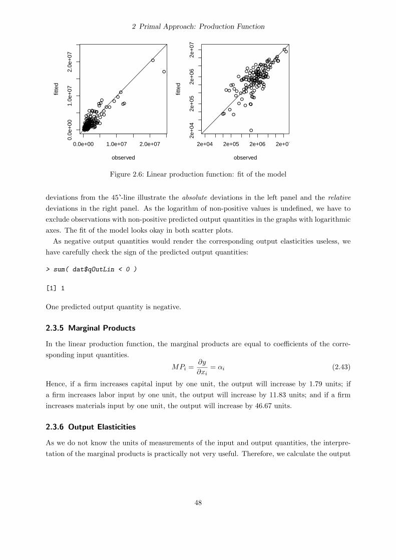
2 Primal Approach: Production Function
●●
●●●
●
●●●●●
●
●●●
●
●
●
●
●
●●●●●
●
●
●
●●●●●
●●
●●● ●●
●●● ●●●●●●●●●●●
●●●●●
●
●●
●
●●
●
●
●
●●
●● ●●●
●
●●●●●
●
●
●
●
●
●● ●
●
●●
●
●
●
●
● ●
●
●
● ●
●●●
●●
●
●●
●●●●
●●
●● ●
●
●● ●
●
●
●●
●
●
●●
●
●
●
●
●
●
●
●
●
0.0e+00 1.0e+07 2.0e+07
0.0e
+00
1.0e
+07
2.0e
+07
observed
fitte
d
●●
●
●
●
●
●● ●●
●
●
●
●●
●
●
●
●
●
●●●
●●
●
●
●
●
●●● ●
● ●
●●
●
●
●
●●
●
●●
●
●
●●●
●●
●
●
● ●●
●
●
●
● ●
●
●
●
●●
●
● ●
●●
●
●
●
●
●
●
●
●
●
●
●
●
●
●
●●
●
●●
●
●
●
●
● ●
●
●
● ●
●●
●
●
●
●
●●
●●
●●
●●
●
●●
●
●● ●
●
●
●
●
●
●
●●
●
●
●
●
●
●
●
●
●
2e+04 2e+05 2e+06 2e+07
2e+
042e
+05
2e+
062e
+07
observed
fitte
dFigure 2.6: Linear production function: fit of the model
deviations from the 45°-line illustrate the absolute deviations in the left panel and the relative
deviations in the right panel. As the logarithm of non-positive values is undefined, we have to
exclude observations with non-positive predicted output quantities in the graphs with logarithmic
axes. The fit of the model looks okay in both scatter plots.
As negative output quantities would render the corresponding output elasticities useless, we
have carefully check the sign of the predicted output quantities:
> sum( dat$qOutLin < 0 )
[1] 1
One predicted output quantity is negative.
2.3.5 Marginal Products
In the linear production function, the marginal products are equal to coefficients of the corre-
sponding input quantities.
MPi = ∂y
∂xi= αi (2.43)
Hence, if a firm increases capital input by one unit, the output will increase by 1.79 units; if
a firm increases labor input by one unit, the output will increase by 11.83 units; and if a firm
increases materials input by one unit, the output will increase by 46.67 units.
2.3.6 Output Elasticities
As we do not know the units of measurements of the input and output quantities, the interpre-
tation of the marginal products is practically not very useful. Therefore, we calculate the output
48

2 Primal Approach: Production Function
elasticities (partial production elasticities) of the three inputs.
εi = ∂y
∂xi
xiy
= MPixiy
= MPiAPi
(2.44)
As the output elasticities depend on the input and output quantities and these quantities generally
differ between firms, also the output elasticities differ between firms. Hence, we can calculate
them for each firm in the sample:
> dat$eCap <- coef(prodLin)["qCap"] * dat$qCap / dat$qOut
> dat$eLab <- coef(prodLin)["qLab"] * dat$qLab / dat$qOut
> dat$eMat <- coef(prodLin)["qMat"] * dat$qMat / dat$qOut
We can obtain their mean values by:
> colMeans( subset( dat, , c( "eCap", "eLab", "eMat" ) ) )
eCap eLab eMat
0.1202721 2.0734793 0.8631936
However, these mean values are distorted by outliers (see figure 2.7). Therefore, we calculate the
median values of the the output elasticities:
> colMedians( subset( dat, , c( "eCap", "eLab", "eMat" ) ) )
eCap eLab eMat
0.08063406 1.28627208 0.58741460
Hence, if a firm increases capital input by one percent, the output will usually increase by around
0.08 percent; if the firm increases labor input by one percent, the output will often increase by
around 1.29 percent; and if the firm increases materials input by one percent, the output will
often increase by around 0.59 percent.
We can visualize (the variation of) these output elasticities with histograms. The user can
modify the desired number of bars in the histogram by adding an integer number as additional
argument:
> hist( dat$eCap )
> hist( dat$eLab, 20 )
> hist( dat$eMat, 20 )
The resulting graphs are shown in figure 2.7. If the firms increase capital input by one percent,
the output of most firms will increase by between 0 and 0.2 percent; if the firms increase labor
input by one percent, the output of most firms will increase by between 0.5 and 3 percent;
and if the firms increase materials input by one percent, the output of most firms will increase
by between 0.2 and 1.2 percent. While the marginal effect of capital on the output is rather
49

2 Primal Approach: Production Function
eCap
Fre
quen
cy
0.0 0.4 0.8 1.2
020
4060
80
eLab
Fre
quen
cy
0 2 4 6 8 10 12 14
010
2030
40
eMat
Fre
quen
cy
0 1 2 3 4 5 6
010
2030
Figure 2.7: Linear production function: output elasticities
small for most firms, there are many firms with implausibly high output elasticities of labor and
materials (εi > 1). This might indicate that the true production technology cannot be reasonably
approximated by a linear production function.
In contrast to a pure theoretical microeconomic model, our empirically estimated model in-
cludes a stochastic error term so that the observed output quantities (y) are not necessarily equal
to the output quantities that are predicted by the model (y = f(x)). This error term comes
from, e.g., measurement errors, omitted explanatory variables, (good or bad) luck, or unusual(ly)
(good or bad) weather conditions. The better the fit of our model, i.e. the higher the R2 value,
the smaller is the difference between the observed and the predicted output quantities. If we
“believe” in our estimated model, it would be more consistent with microeconomic theory, if we
use the predicted output quantities and disregard the stochastic error term.
We can calculate the output elasticities based on the predicted output quantities (see sec-
tion 2.3.4) rather than the observed output quantities:
> dat$eCapFit <- coef(prodLin)["qCap"] * dat$qCap / dat$qOutLin
> dat$eLabFit <- coef(prodLin)["qLab"] * dat$qLab / dat$qOutLin
> dat$eMatFit <- coef(prodLin)["qMat"] * dat$qMat / dat$qOutLin
> colMeans( subset( dat, , c( "eCapFit", "eLabFit", "eMatFit" ) ) )
eCapFit eLabFit eMatFit
0.1421941 2.2142092 0.9784056
> colMedians( subset( dat, , c( "eCapFit", "eLabFit", "eMatFit" ) ) )
eCapFit eLabFit eMatFit
0.07407719 1.21044421 0.58821500
> hist( dat$eCapFit, 20 )
> hist( dat$eLabFit, 20 )
> hist( dat$eMatFit, 20 )
50

2 Primal Approach: Production Function
eCapFit
Fre
quen
cy
0.0 0.5 1.0 1.5 2.0 2.5 3.0
020
4060
8010
0
eLabFit
Fre
quen
cy
−10 0 10 20 30 40 50
020
4060
8012
0
eMatFit
Fre
quen
cy
−5 0 5 10 15 20 25
020
4060
8010
0
Figure 2.8: Linear production function: output elasticities based on predicted output quantities
The resulting graphs are shown in figure 2.8. While the choice of the variable for the output
quantity (observed vs. predicted) only has a minor effect on the mean and median values of the
output elasticities, the ranges of the output elasticities that are calculated from the predicted
output quantities are much larger than the ranges of the output elasticities that are calculated
from the observed output quantities. Due to 1 negative predicted output quantity, the output
elasticities of this observation are also negative.
2.3.7 Elasticity of Scale
The elasticity of scale is the sum of all output elasticities
ε =∑i
εi (2.45)
Hence, the elasticities of scale of all firms in the sample can be calculated by:
> dat$eScale <- with( dat, eCap + eLab + eMat )
> dat$eScaleFit <- with( dat, eCapFit + eLabFit + eMatFit )
The mean and median values of the elasticities of scale can be calculated by
> colMeans( subset( dat, , c( "eScale", "eScaleFit" ) ) )
eScale eScaleFit
3.056945 3.334809
> colMedians( subset( dat, , c( "eScale", "eScaleFit" ) ) )
eScale eScaleFit
1.941536 1.864253
Hence, if a firm increases all input quantities by one percent, the output quantity will usually
increase by around 1.9 percent. This means that most firms have increasing returns to scale and
51
2 Primal Approach: Production Function
hence, the firms could increase productivity by increasing the firm size (i.e. increasing all input
quantities).
The (variation of the) elasticities of scale can be visualized with histograms:
> hist( dat$eScale, 30 )
> hist( dat$eScaleFit, 50 )
> hist( dat$eScaleFit[ dat$eScaleFit > 0 & dat$eScaleFit < 15 ], 30 )
eScale
Fre
quen
cy
0 5 10 15
05
1015
2025
30
eScaleFit
Fre
quen
cy
0 20 40 60 80
020
4060
0 < eScaleFit < 15
Fre
quen
cy
2 4 6 8 10 12 14
010
2030
40
Figure 2.9: Linear production function: elasticities of scale
The resulting graphs are shown in figure 2.9. As the predicted output quantity of 1 firm is nega-
tive, the elasticity of scale of this observation also is negative, if the predicted output quantities
are used for the calculation. However, all remaining elasticities of scale that are based on the
predicted output quantities are larger than one, which indicates increasing returns to scale. In
contrast, 15 (out of 140) elasticities of scale that are calculated with the observed output quanti-
ties indicate decreasing returns to scale. However, both approaches indicate that most firms have
an elasticity of scale between one and two. Hence, if these firms increase all input quantities by
one percent, the output of most firms will increase by between 1 and 2 percent. Some firms even
have an elasticity of scale larger than five, which is very implausible and might indicate that the
true production technology cannot be reasonably approximated by a linear production function.
Information on the optimal firm size can be obtained by analyzing the interrelationship between
firm size and the elasticity of scale:
> plot( dat$qOut, dat$eScale, log = "x" )
> abline( 1, 0 )
> plot( dat$X, dat$eScale, log = "x" )
> abline( 1, 0 )
> plot( dat$qOut, dat$eScaleFit, log = "x", ylim = c( 0, 15 ) )
> abline( 1, 0 )
> plot( dat$X, dat$eScaleFit, log = "x", ylim = c( 0, 15 ) )
> abline( 1, 0 )
52

2 Primal Approach: Production Function
●●
●
●
● ●
●
●●
●
● ●● ●
●
●
●
●
●
● ●●
●
●
●
●●
●
●
● ●
●
●
●
●●
●
●
●●
● ●
●
●
●
●●
●
●●
●●
●
●
●
●
●
●
●
●
●
●
●
●
●
●
●●
●
●●●
●
●
●
●
●
●
●
●
● ●
●●
●●
●
●
● ●●●
●
●●
●
●
●
●
●
●
●
●
●
●
●
●
●
●●● ●
●●
●
●
●
●
●
●
●
●
●●
●●
● ●
●●
●
●● ●●
●
●●● ●
0.5 1.0 2.0 5.0
510
15
X
eSca
le
●●
●
●
● ●
●
●●
●
● ●● ●
●
●
●
●
●
● ●●
●
●
●
●●
●
●
●●
●
●
●
●●
●
●
●●
●●
●
●
●
●●●
●●●
●
●
●
●
●
●
●
●
●
●
●
●
●
●
●
●●
●
●●●
●
●
●
●
●
●
●
●
● ●
●●
●●
●
●
● ●●●
●
●●
●
●
●
●
●
●
●
●
●
●
●
●
●
●●● ●
●●
●
●
●
●
●
●
●
●
●●
●●
● ●
●●
●
●● ●●
●
●●● ●
1e+05 5e+05 2e+06 5e+06 2e+07
510
15
qOut
eSca
le
●●
●
●
●
●●●● ●
●
●
●●●
●
●
●
●
●●●●●●
●
●
●
●
● ●●●● ●
●
●
●
●
●
● ●●
●●
●
●
●●●
●
●
●
●●●
●
●
●
● ●
●
●●
●●●
● ●
●
●
●
●
●
●
●
●
●
●
●
●
●● ●●
●●
●
●●● ●
●
●
● ●●
●
● ●● ● ●
●●
●
●●● ●
●●
●●
●●●
●● ●●
●●
●
●
●
●
● ●●
●
●
●
●
●●
●
●
0.5 1.0 2.0 5.0
05
1015
X
eSca
leF
it
●●
●
●
●
●●● ●●
●
●
●●●
●
●
●
●
●●●● ●●
●
●
●
●
●●● ●● ●
●
●
●
●
●
●●●
●●
●
●
●●●
●
●
●
● ●●
●
●
●
● ●
●
●●
●●●
● ●
●
●
●
●
●
●
●
●
●
●
●
●
●●●●
●●
●
●●●●
●
●
● ●●
●
● ●●● ●
●●
●
●●● ●
●●
●●
●● ●●
●● ●
●●
●
●
●
●
●●●
●
●
●
●
●●
●
●
1e+05 5e+05 2e+06 5e+06 2e+07
05
1015
qOut
eSca
leF
it
Figure 2.10: Linear production function: elasticities of scale for different firm sizes
53

2 Primal Approach: Production Function
The resulting graphs are shown in figure 2.10. They indicate that very small firms could enor-
mously gain from increasing their size, while the benefits from increasing firm size decrease with
size. Only a few elasticities of scale that are calculated with the observed output quantities indi-
cate decreasing returns to scale so that productivity would decline when these firms increase their
size. For all firms that use at least 2.1 times the input quantities of the average firm or produces
more than 6,000,000 quantity units (approximately 6,000,000 Euros), the elasticities of scale that
are based on the observed input quantities are very close to one. From this observation we could
conclude that firms have their optimal size when they use at least 2.1 times the input quantities
of the average firm or produce at least 6,000,000 quantity units (approximately 6,000,000 Euros
turn over). In contrast, the elasticities of scale that are based on the predicted output quantities
are larger one even for the largest firms in the data set. From this observation, we could conclude
that the even the largest firms in the sample would gain from growing in size and thus, the most
productive scale size is lager than the size of the largest firms in the sample.
The high elasticities of scale explain why we found much higher partial productivities (average
products) and total factor productivities for larger firms than for smaller firms.
2.3.8 Marginal rates of technical substitution
As the marginal products based on a linear production function are equal to the coefficients, we
can calculate the MRTS (2.7) as follows:
> mrtsCapLab <- - coef(prodLin)["qLab"] / coef(prodLin)["qCap"]
qLab
-6.615934
> mrtsLabCap <- - coef(prodLin)["qCap"] / coef(prodLin)["qLab"]
qCap
-0.1511502
> mrtsCapMat <- - coef(prodLin)["qMat"] / coef(prodLin)["qCap"]
qMat
-26.09666
> mrtsMatCap <- - coef(prodLin)["qCap"] / coef(prodLin)["qMat"]
qCap
-0.03831908
> mrtsLabMat <- - coef(prodLin)["qMat"] / coef(prodLin)["qLab"]
54

2 Primal Approach: Production Function
qMat
-3.944516
> mrtsMatLab <- - coef(prodLin)["qLab"] / coef(prodLin)["qMat"]
qLab
-0.2535165
Hence, if a firm wants to reduce the use of labor by one unit, he/she has to use 6.62 additional
units of capital in order to produce the same output as before. Alternatively, the firm can replace
the unit of labor by using 0.25 additional units of materials. If the firm increases the use of labor
by one unit, he/she can reduce capital by 6.62 units whilst still producing the same output as
before. Alternatively, the firm can reduce materials by 0.25 units.
2.3.9 Relative marginal rates of technical substitution
We can calculate the RMRTS (2.8) derived from the linear production function as follows:
> dat$rmrtsCapLab <- - dat$eLab / dat$eCap
> dat$rmrtsLabCap <- - dat$eCap / dat$eLab
> dat$rmrtsCapMat <- - dat$eMat / dat$eCap
> dat$rmrtsMatCap <- - dat$eCap / dat$eMat
> dat$rmrtsLabMat <- - dat$eMat / dat$eLab
> dat$rmrtsMatLab <- - dat$eLab / dat$eMat
We can visualize (the variation of) these RMRTSs with histograms:
> hist( dat$rmrtsCapLab, 20 )
> hist( dat$rmrtsLabCap )
> hist( dat$rmrtsCapMat )
> hist( dat$rmrtsMatCap )
> hist( dat$rmrtsLabMat )
> hist( dat$rmrtsMatLab )
The resulting graphs are shown in figure 2.11. According to the RMRTS based on the linear
production function, most firms need between 20% more capital or around 2% more materials to
compensate a 1% reduction of labor.
2.3.10 First-order conditions for profit maximisation
In this section, we will check to what extent the first-order conditions for profit maximization
(2.24) are fulfilled, i.e. to what extent the firms use the optimal input quantities. We do this by
comparing the marginal value products of the inputs with the corresponding input prices. We
can calculate the marginal value products by multiplying the marginal products by the output
price:
55

2 Primal Approach: Production Function
rmrtsCapLab
Fre
quen
cy
−150 −100 −50 0
010
2030
4050
rmrtsLabCap
Fre
quen
cy
−0.20 −0.10 0.00
010
2030
rmrtsCapMat
Fre
quen
cy
−60 −40 −20 0
010
2030
4050
60
rmrtsMatCap
Fre
quen
cy
−0.5 −0.4 −0.3 −0.2 −0.1 0.0
010
2030
40
rmrtsLabMat
Fre
quen
cy
−1.5 −1.0 −0.5 0.0
010
2030
4050
rmrtsMatLab
Fre
quen
cy
−8 −6 −4 −2 0
010
2030
4050
Figure 2.11: Linear production function: relative marginal rates of technical substitution(RMRTS)
56

2 Primal Approach: Production Function
> dat$mvpCap <- dat$pOut * coef(prodLin)["qCap"]
> dat$mvpLab <- dat$pOut * coef(prodLin)["qLab"]
> dat$mvpMat <- dat$pOut * coef(prodLin)["qMat"]
The command compPlot (package miscTools) can be used to compare the marginal value products
with the corresponding input prices:
> compPlot( dat$pCap, dat$mvpCap )
> compPlot( dat$pLab, dat$mvpLab )
> compPlot( dat$pMat, dat$mvpMat )
> compPlot( dat$pCap, dat$mvpCap, log = "xy" )
> compPlot( dat$pLab, dat$mvpLab, log = "xy" )
> compPlot( dat$pMat, dat$mvpMat, log = "xy" )
●●
●
●
●
●●
●
●
●
●●
●
●●
●
●●
●
●
●
●
●
●
● ●
● ●
● ●●
●
●
●●
●
● ●
●
●
●
●
●
●
●
●● ●●
●●
● ● ●●
●
●
●
● ●●
●
●
●
●
●
●●
●
●
●
●
●
●
●● ●●● ●
●
●
●
●
●●
●
●
●
●
●●
●
●
●●
●●
●
●
●●
●
●
●
● ●●
●
●
●●
●●
●
●
●
●
●
●
●
● ●
●
●
●
●
●
●
●
●
●
●
●
●●
●
●
●
●
0 1 2 3 4 5
01
23
45
w Cap
MV
P C
ap
●●
●
●
●
●●
●
●
●
●●
●
●●
●
●●
●
●
●
●
●
●
●●
●●
●●●●
●
●●●
●●
●
●
●
●
●
●
●
●●●●●●
●●●●
●
●
●
●●●
●
●
●
●
●
●●
●
●
●
●
●
●
●●●●●●
●
●
●
●
●●
●
●
●
●
●●
●
●
●●
●●
●
●
●●
●
●
●
●●●
●
●
●●
●●
●
●
●
●
●
●
●
●●
●
●
●
●
●
●
●
●
●
●
●
●●
●
●
●
●
0 5 10 15 20 25 30 35
05
1015
2025
3035
w Lab
MV
P L
ab
●●
●
●
●
●●
●
●
●
●●
●
●●
●
●●
●
●
●
●
●
●
●●
●●
●●●
●
●
●●●
●●
●
●
●
●
●
●
●
●●●●
●●
●●●●
●
●
●
● ●●
●
●
●
●
●
●●
●
●
●
●
●
●
●●●●●●
●
●
●
●
●●
●
●
●
●
●●
●
●
●●
●●
●
●
●●
●
●
●
●●●
●
●
●●
●●
●
●
●
●
●
●
●
●●
●
●
●
●
●
●
●
●
●
●
●
●●
●
●
●
●
0 20 40 60 80 120
020
4060
8010
014
0
w Mat
MV
P M
at
●●
●
●
●
●●
●
●
●
●●
●
● ●
●
●●
●
●
●
●
●
●
● ●
● ●
● ●●
●
●
●●
●
● ●
●
●
●
●
●
●
●
●● ●
●●
●
● ● ●●
●
●
●
● ●●
●
●
●
●
●
●●
●
●
●
●
●
●
●● ●●● ●
●
●
●
●
●●
●
●
●
●
●●
●●
●●
●●
●
●
●●
●
●
●
● ●●
●
●
●●
●●
●
●
●
●
●
●
●
● ●
●
●
●
●
●
●
●
●
●
●●
●●
●
●
●
●
0.2 0.5 1.0 2.0 5.0
0.2
0.5
1.0
2.0
5.0
w Cap
MV
P C
ap
●●
●
●
●
●●
●
●
●
●●
●
● ●
●
●●
●
●
●
●
●
●
●●
●●
●●●●
●
●●
●
●●
●
●
●
●
●
●
●
●●●
●●●
●●●●
●
●
●
● ●●
●
●
●
●
●
●●
●
●
●
●
●
●● ●●●●●
●
●
●
●●●
●●
●
●
●●
●●
● ●
● ●
●
●
●●
●
●
●
● ●●
●
●
●●
●●
●
●
●
●
●
●
●
●●
●
●
●
●
●
●
●
●
●
●●
●●
●
●
●
●
0.5 1.0 2.0 5.0 20.0
0.5
1.0
2.0
5.0
10.0
w Lab
MV
P L
ab
●●
●
●
●
●●
●
●
●
● ●
●
●●
●
●●
●
●
●
●
●
●
●●
●●
● ●●
●
●
●●
●
●●
●
●
●
●
●
●
●
●●●
●●
●
●●● ●
●
●
●
● ●●
●
●
●
●
●
●●
●
●
●
●
●
●● ●● ●●●
●
●
●
●
● ●
●
●
●
●
●●
●●
● ●
●●
●
●
●●
●
●
●
●●●
●
●
●●
●●
●
●
●
●
●
●
●
● ●
●
●
●
●
●
●
●
●
●
●●
●●
●
●
●
●
5 10 20 50 100
510
2050
100
w Mat
MV
P M
at
Figure 2.12: Marginal value products and corresponding input prices
The resulting graphs are shown in figure 2.12. The graphs on the left side indicate that the
marginal value products of capital are sometimes lower but more often higher than the capital
prices. The four other graphs indicate that the marginal value products of labor and materials
are always higher than the labor prices and the materials prices, respectively. This indicates that
57

2 Primal Approach: Production Function
some firms could increase their profit by using more capital and all firms could increase their
profit by using more labor and more materials. Given that most firms operate under increasing
returns to scale, it is not surprising that most firms would gain from increasing most—or even
all—input quantities. Therefore, the question arises why the firms in the sample did not do this.
There are many possible reasons for not increasing the input quantities until the predicted op-
timal input levels, e.g. legal restrictions, environmental regulations, market imperfections, credit
(liquidity) constraints, and/or risk aversion. Furthermore, market imperfections might cause that
the (observed) average prices are lower than the marginal costs of obtaining these inputs (e.g.
Henning and Henningsen, 2007), particularly for labor and capital.
2.3.11 First-order conditions for cost minimization
As the marginal rates of technical substitution are constant for linear production functions, we
compare the input price ratios with the negative inverse marginal rates of technical substitution
by creating a histogram for each input price ratio and drawing a vertical line at the corresponding
negative marginal rate of technical substitution:
> hist( dat$pCap / dat$pLab )
> lines( rep( - mrtsLabCap, 2), c( 0, 100 ), lwd = 3 )
> hist( dat$pCap / dat$pMat )
> lines( rep( - mrtsMatCap, 2), c( 0, 100 ), lwd = 3 )
> hist( dat$pLab / dat$pMat )
> lines( rep( - mrtsMatLab, 2), c( 0, 100 ), lwd = 3 )
> hist( dat$pLab / dat$pCap )
> lines( rep( - mrtsCapLab, 2), c( 0, 100 ), lwd = 3 )
> hist( dat$pMat / dat$pCap )
> lines( rep( - mrtsCapMat, 2), c( 0, 100 ), lwd = 3 )
> hist( dat$pMat / dat$pLab )
> lines( rep( - mrtsLabMat, 2), c( 0, 100 ), lwd = 3 )
The resulting graphs are shown in figure 2.13. The upper left graph shows that the ratio between
the capital price and the labor price is larger than the absolute value of the marginal rate of
technical substitution between labor and capital (0.151) for the most firms in the sample:
wcapwlab
> −MRTSlab,cap = MPcapMPlab
(2.46)
Or taken the other way round, the lower left graph shows that the ratio between the labor
price and the capital price is smaller than the absolute value of the marginal rate of technical
substitution between capital and labor (6.616) for the most firms in the sample:
wlabwcap
< −MRTScap,lab = MPlabMPcap
(2.47)
58

2 Primal Approach: Production Function
w Cap / w Lab
Fre
quen
cy
0 1 2 3 4 5
010
2030
40
w Cap / w Mat
Fre
quen
cy
0.0 0.2 0.4 0.6 0.8
010
2030
4050
w Lab / w Mat
Fre
quen
cy
0.1 0.2 0.3 0.4
010
2030
40
w Lab / w Cap
Fre
quen
cy
0 2 4 6 8
020
4060
80
w Mat / w Cap
Fre
quen
cy
0 10 20 30 40 50 60
010
2030
4050
60
w Mat / w Lab
Fre
quen
cy
5 10 15 20
010
2030
40
Figure 2.13: First-order conditions for costs minimization
59

2 Primal Approach: Production Function
Hence, the firm can get closer to the minimum of the costs by substituting labor for capital,
because this will decrease the marginal product of labor and increase the marginal product of
capital so that the absolute value of the MRTS between labor and capital increases, the absolute
value of the MRTS between capital and labor decreases, and both of the MRTS get closer to the
corresponding input price ratios. Similarly, the graphs in the middle column indicate that almost
all firms should substitute materials for capital and the graphs on the right indicate that most of
the firms should substitute labor for materials. Hence, the firms could reduce production costs
particularly by using less capital and more labor.
2.3.12 Derived Input Demand Functions and Output Supply Functions
Given a linear production function (2.42), the input quantities chosen by a profit maximizing
producer are either zero, indeterminate, or infinity:
xi(p, w) =
0 if MV Pi < wi
indeterminate if MV Pi = wi
∞ if MV Pi > wi
(2.48)
If all input quantities are zero, the output quantity is equal to the intercept, which is zero in case
of weak essentiality. Otherwise, the output quantity is indeterminate or infinity:
y(p, w) =
β0 if MV Pi < wi ∀ i
∞ if MV Pi > wi ∃ i
indeterminate otherwise
(2.49)
A cost minimizing producer will use only a single input, i.e. the input with the lowest cost
per unit of produced output (wi/MPi). If the lowest cost per unit of produced output can be
obtained by two or more inputs, these input quantities are indeterminate.
xi(w, y) =
0 if βi
wi<
βjwj∃ j
y−β0βi
if βiwi>
βjwj∀ j 6= i
indeterminate otherwise
(2.50)
Given that the unconditional and conditional input demand functions and the output supply
functions based on the linear production function are non-continuous and often return either zero
or infinite values, it does not make much sense to use this functional form to predict the effects
of price changes when the true technology implies that firms always use non-zero finite input
quantities.
60

2 Primal Approach: Production Function
2.4 Cobb-Douglas production function
2.4.1 Specification
A Cobb-Douglas production function with N inputs is defined as:
y = AN∏i=1
xαii . (2.51)
This function can be linearized by taking the (natural) logarithm on both sides:
ln y = α0 +N∑i=1
αi ln xi, (2.52)
where α0 is equal to lnA.
2.4.2 Estimation
We can estimate this Cobb-Douglas production function for our data set using the command lm:
> prodCD <- lm( log( qOut ) ~ log( qCap ) + log( qLab ) + log( qMat ),
+ data = dat )
> summary( prodCD )
Call:
lm(formula = log(qOut) ~ log(qCap) + log(qLab) + log(qMat), data = dat)
Residuals:
Min 1Q Median 3Q Max
-1.67239 -0.28024 0.00667 0.47834 1.30115
Coefficients:
Estimate Std. Error t value Pr(>|t|)
(Intercept) -2.06377 1.31259 -1.572 0.1182
log(qCap) 0.16303 0.08721 1.869 0.0637 .
log(qLab) 0.67622 0.15430 4.383 2.33e-05 ***
log(qMat) 0.62720 0.12587 4.983 1.87e-06 ***
---
Signif. codes: 0 ‘***’ 0.001 ‘**’ 0.01 ‘*’ 0.05 ‘.’ 0.1 ‘ ’ 1
Residual standard error: 0.656 on 136 degrees of freedom
Multiple R-squared: 0.5943, Adjusted R-squared: 0.5854
F-statistic: 66.41 on 3 and 136 DF, p-value: < 2.2e-16
61

2 Primal Approach: Production Function
2.4.3 Properties
The monotonicity condition is (globally) fulfilled, as the estimated coefficients of all three (loga-
rithmic) input quantities are positive and the output quantity as well as all input quantities are
non-negative (see equation 2.54). However, the coefficient of the (logarithmic) capital quantity is
only statistically significantly different from zero at the 10% level. Therefore, we cannot be sure
that the capital quantity has a positive effect on the output quantity.
The quasi-concavity of our estimated Cobb-Douglas production function is checked in sec-
tion 2.4.12.
The production technology described by a Cobb-Douglas production function always shows
weak and strict essentiality, because the output quantity becomes zero, as soon as a single input
quantity becomes zero (see equation 2.51).
The input requirement sets derived from Cobb-Douglas production functions are always closed
and non-empty for y > 0 if strict monotonicity is fulfilled for at least one input (∃ i ∈ {1, . . . , N} :βi > 0), as the input quantities must be non-negative (xi ≥ 0 ∀ i).
The Cobb-Douglas production function always returns finite, real, and single values if the input
quantities are non-negative and finite. The predicted output quantity is non-negative as long as
A and the input quantities are non-negative, where A = exp(α0) is positive even if α0 is negative.
All Cobb-Douglas production functions are continuous and twice-continuously differentiable.
2.4.4 Predicted output quantities
We can calculate the predicted (“fitted”) output quantities manually by taking the Cobb-Douglas
function (2.51), the observed input quantities, and the estimated parameters, but it is easier
to use the fitted method to obtain the predicted values of the dependent variable from an
estimated model. As we estimated the Cobb-Douglas function in logarithms, we have to use the
exponential function to obtain the predicted values in levels (non-logarithms):
> dat$qOutCD <- exp( fitted( prodCD ) )
> all.equal( dat$qOutCD,
+ with( dat, exp( coef( prodCD )[ "(Intercept)" ] ) *
+ qCap^coef( prodCD )[ "log(qCap)" ] *
+ qLab^coef( prodCD )[ "log(qLab)" ] *
+ qMat^coef( prodCD )[ "log(qMat)" ] ) )
[1] TRUE
We can evaluate the “fit” of the Cobb-Douglas production function by comparing the observed
with the fitted output quantities:
> compPlot( dat$qOut, dat$qOutCD )
> compPlot( dat$qOut, dat$qOutCD, log = "xy" )
62

2 Primal Approach: Production Function
●●
●●●
●
●●●●●
●
●●●
●
●
●
●●
●●●●●●
●
●
● ●●●●●●
●●● ●●●●● ●●
●●●●●●●●●
●●●●●
●
●●
●
●●
●●
●
●
●
●● ●●●
●●
●●●●
●
●
●
●
●
●● ●
●
●●
●
●
●
●
●●
●
●
●●
●● ●●
●
●
●
●
●●●●
●●●● ●
●
●● ●
●●
●●●
●
●●
●
●
●
●●
●
●
●
●
0.0e+00 1.0e+07 2.0e+07
0.0e
+00
1.0e
+07
2.0e
+07
observed
fitte
d
●●
●
● ●
●
●●
●●
●
●
●
●●
●
●
●
●
●
●●
● ●●●
●
●
●
●●
● ●
●●
●
●
●
●
●
●●
●●●
●
●
●●
●●
●●
●
● ●●
●●
●
●
●
●
●
●
●●
●
●
●
●● ●
●
●
●
●
●
●
●
●
●
●
●
●
●
●
●●
●
●●
●
●
●
●
●
●
●
●
●●
●●
●
●
●
●
●
●
●
●
●●
●
●
●● ●
●
●● ●
●●
●
●
●
●
●●
●
●
●
●
●
●
●
●
●
1e+05 5e+05 5e+06
1e+
055e
+05
2e+
061e
+07
observed
fitte
dFigure 2.14: Cobb-Douglas production function: fit of the model
The resulting graphs are shown in figure 2.14. While the graph in the left panel uses a linear
scale for the axes, the graph in the right panel uses a logarithmic scale for both axes. Hence, the
deviations from the 45°-line illustrate the absolute deviations in the left panel and the relative
deviations in the right panel. The fit of the model looks okay in the scatter plot on the left-hand
side, but if we use a logarithmic scale on both axes (as in the graph on the right-hand side), we
can see that the output quantity is generally over-estimated if the the observed output quantity
is small.
2.4.5 Output elasticities
In the Cobb-Douglas function, the output elasticities of the inputs are equal to the corresponding
coefficients.
εi = ∂y
∂xi
xiy
= ∂ ln y∂ ln xi
= αi (2.53)
Hence, if a firm increases capital input by one percent, the output will increase by 0.16 percent;
if a firm increases labor input by one percent, the output will increase by 0.68 percent; and if
a firm increases materials input by one percent, the output will increase by 0.63 percent. The
output elasticity of capital is somewhat larger and the output elasticity of labor is considerably
smaller when estimated by a Cobb-Douglas production function than when estimated by a linear
production function. Indeed, the output elasticities of all three inputs are in the reasonable range,
i.e. between zero one one, now.
2.4.6 Marginal products
In the Cobb-Douglas function, the marginal products of the inputs can be calculated by following
formula:∂y
∂xi= ∂ ln y∂ ln xi
y
xi= βi
y
xi= βi APi (2.54)
63

2 Primal Approach: Production Function
As the marginal products depend on the input and output quantities and these quantities gener-
ally differ between firms, the marginal products based on Cobb-Douglas also differ between firms.
Hence, we can calculate them for each firm in the sample:
> dat$mpCapCD <- coef(prodCD)["log(qCap)"] * dat$apCap
> dat$mpLabCD <- coef(prodCD)["log(qLab)"] * dat$apLab
> dat$mpMatCD <- coef(prodCD)["log(qMat)"] * dat$apMat
We can visualize (the variation of) these marginal products with histograms:
> hist( dat$mpCapCD )
> hist( dat$mpLabCD )
> hist( dat$mpMatCD )
MP Cap
Fre
quen
cy
0 5 10 15 20 25
010
2030
4050
MP Lab
Fre
quen
cy
0 5 10 15
05
1015
2025
30
MP Mat
Fre
quen
cy
0 50 100 150 2000
1020
30
Figure 2.15: Cobb-Douglas production function: marginal products
The resulting graphs are shown in figure 2.15. If the firms increase capital input by one unit, the
output of most firms will increase by between 0 and 8 units; if the firms increase labor input by
one unit, the output of most firms will increase by between 2 and 12 units; and if the firms increase
materials input by one unit, the output of most firms will increase by between 20 and 80 units.
Not surprisingly, a comparison of these marginal effects with the marginal effects from the linear
production function confirms the results from the comparison based on the output elasticities:
the marginal products of capital are generally larger than the marginal product estimated by
the linear production function and the marginal products of labor are generally smaller than the
marginal product estimated by the linear production function, while the marginal products of
fuel are (on average) rather similar to the marginal product estimated by the linear production
function.
2.4.7 Elasticity of Scale
As the elasticity of scale is the sum of all output elasticities (see equation 2.45), we can calculate
it simply by summing up all coefficients except for the intercept:
64

2 Primal Approach: Production Function
> sum( coef( prodCD )[ -1 ] )
[1] 1.466442
Hence, if the firm increases all input quantities by one percent, output will increase by 1.47
percent. This means that the technology has strong increasing returns to scale. However, in
contrast to the results of the linear production function, the elasticity of scale based on the Cobb-
Douglas production function is (globally) constant. Hence, it does not decrease (or increase), e.g.,
with the size of the firm. This means that the optimal firm size would be infinity.
We can use the delta method (see section 1.4.3) to calculate the variance and the standard error
of the elasticity of scale. Given that the first derivatives of the elasticity of scale with respect to
the estimated coefficients are ∂ε/∂α0 = 0 and ∂ε/∂αCap = ∂ε/∂αLab = ∂ε/∂αMat = 1, we can
do this by following commands:
> ESCD <- sum( coef(prodCD)[-1] )
[1] 1.466442
> dESCD <- c( 0, 1, 1, 1 )
[1] 0 1 1 1
> varESCD <- t(dESCD) %*% vcov(prodCD) %*% dESCD
[,1]
[1,] 0.0118237
> seESCD <- sqrt( varESCD )
[,1]
[1,] 0.1087369
Now, we can apply a t test to test whether the elasticity of scale significantly differs from one.
The following commands calculate the t value and the critical value for a two-sided t test based
on a 5% significance level:
> tESCD <- (ESCD - 1) / seESCD
[,1]
[1,] 4.289645
> cvESCD <- qt( 0.975, 136 )
[1] 1.977561
65

2 Primal Approach: Production Function
Given that the t value is larger than the critical value, we can reject the null hypothesis of
constant returns to scale and conclude that the technology has significantly increasing returns to
scale. The P value for this two-sided t test is:
> pESCD <- 2 * ( 1 - pt( tESCD, 136 ) )
[,1]
[1,] 3.372264e-05
Given that the P value is close to zero, we can be very sure that the technology has increasing
returns to scale. The 95% confidence interval for the elasticity of scale is:
> c( ESCD - cvESCD * seESCD, ESCD + cvESCD * seESCD )
[1] 1.251409 1.681476
2.4.8 Marginal Rates of Technical Substitution
The MRTS based on the Cobb-Douglas production function differ between firms. They can be
calculated as follows:
> dat$mrtsCapLabCD <- - dat$mpLabCD / dat$mpCapCD
> dat$mrtsLabCapCD <- - dat$mpCapCD / dat$mpLabCD
> dat$mrtsCapMatCD <- - dat$mpMatCD / dat$mpCapCD
> dat$mrtsMatCapCD <- - dat$mpCapCD / dat$mpMatCD
> dat$mrtsLabMatCD <- - dat$mpMatCD / dat$mpLabCD
> dat$mrtsMatLabCD <- - dat$mpLabCD / dat$mpMatCD
We can visualize (the variation of) these MRTSs with histograms:
> hist( dat$mrtsCapLabCD )
> hist( dat$mrtsLabCapCD )
> hist( dat$mrtsCapMatCD )
> hist( dat$mrtsMatCapCD )
> hist( dat$mrtsLabMatCD )
> hist( dat$mrtsMatLabCD )
The resulting graphs are shown in figure 2.16. According to the MRTS based on the Cobb-
Douglas production function, most firms only need between 0.5 and 2 additional units of capital
or between 0.05 and 0.15 additional units of materials to replace one unit of labor.
66

2 Primal Approach: Production Function
mrtsCapLabCD
Fre
quen
cy
−6 −5 −4 −3 −2 −1 0
05
1015
2025
3035
mrtsLabCapCD
Fre
quen
cy
−6 −5 −4 −3 −2 −1 0
010
2030
4050
60
mrtsCapMatCD
Fre
quen
cy
−50 −40 −30 −20 −10 0
010
2030
mrtsMatCapCD
Fre
quen
cy
−0.6 −0.4 −0.2 0.0
010
2030
4050
60
mrtsLabMatCD
Fre
quen
cy
−35 −25 −15 −5 0
010
2030
4050
60
mrtsMatLabCD
Fre
quen
cy
−0.4 −0.3 −0.2 −0.1 0.0
010
2030
4050
Figure 2.16: Cobb-Douglas production function: marginal rates of technical substitution (MRTS)
2.4.9 Relative Marginal Rates of Technical Substitution
As we do not know the units of measurements of the input quantities, the interpretation of
the MRTSs is practically not very useful. To overcome this problem, we calculate the relative
marginal rates of technical substitution (RMRTS) by equation (2.8). As the output elasticities
based on a Cobb-Douglas production function are equal to the coefficients, we can calculate the
RMRTS as follows:
> rmrtsCapLabCD <- - coef(prodCD)["log(qLab)"] / coef(prodCD)["log(qCap)"]
log(qLab)
-4.147897
> rmrtsLabCapCD <- - coef(prodCD)["log(qCap)"] / coef(prodCD)["log(qLab)"]
log(qCap)
-0.241086
> rmrtsCapMatCD <- - coef(prodCD)["log(qMat)"] / coef(prodCD)["log(qCap)"]
log(qMat)
-3.847203
67
2 Primal Approach: Production Function
> rmrtsMatCapCD <- - coef(prodCD)["log(qCap)"] / coef(prodCD)["log(qMat)"]
log(qCap)
-0.2599291
> rmrtsLabMatCD <- - coef(prodCD)["log(qMat)"] / coef(prodCD)["log(qLab)"]
log(qMat)
-0.9275069
> rmrtsMatLabCD <- - coef(prodCD)["log(qLab)"] / coef(prodCD)["log(qMat)"]
log(qLab)
-1.078159
Hence, if a firm wants to reduce the use of labor by one percent, it has to use 4.15 percent more
capital in order to produce the same output as before. Alternatively, the firm can replace one
percent of labor by using 1.08 percent more materials. If the firm increases the use of labor by one
percent, it can reduce capital by 4.15 percent whilst still producing the same output as before.
Alternatively, the firm can reduce materials by 1.08 percent.
2.4.10 First and second partial derivatives
For the Cobb-Douglas production function with three inputs (2.51), the first derivatives (marginal
products) are
f1 = ∂y
∂x1= α1 A xα1−1
1 xα22 xα3
3 = α1y
x1(2.55)
f2 = ∂y
∂x2= α2 A xα1
1 xα2−12 xα3
3 = α2y
x2(2.56)
f3 = ∂y
∂x3= α3 A xα1
1 xα22 xα3−1
3 = α3y
x3(2.57)
and the second derivatives are
f11 = ∂f1∂x1
= α1f1x1− α1
y
x21
= f21y− f1x1
(2.58)
f22 = ∂f2∂x2
= α2f2x2− α2
y
x22
= f22y− f2x2
(2.59)
f33 = ∂f3∂x3
= α3f3x3− α3
y
x23
= f23y− f3x3
(2.60)
f12 = ∂f1∂x2
= α1f2x1
= f1 f2y
(2.61)
f13 = ∂f1∂x3
= α1f3x1
= f1 f3y
(2.62)
68

2 Primal Approach: Production Function
f23 = ∂f2∂x3
= α2f3x2
= f2 f3y
. (2.63)
Generally, for an N -input Cobb-Douglas function, the first and second derivatives are
fi = αiy
xi(2.64)
fij = fi fjy− δij
fixi, (2.65)
where δij denotes Kronecker’s delta with
δij =
1 if i = j
0 if i 6= j(2.66)
In the calculations of the partial derivatives (fi), we have simplified the formulas by replacing
the right-hand side of the Cobb-Douglas function (2.51) by the output quantities. When we
calculated the marginal products (partial derivatives) of the Cobb-Douglas function in in sec-
tion 2.4.6, we have used the observed output quantities for y. However, as the fit (R2 value)
of our model is not 100 %, the observed output quantities are generally not equal to the output
quantities predicted by our model, i.e. the right-hand side of the Cobb-Douglas function (2.51)
using the estimated parameters. The better the fit of our model, the smaller is the difference
between the observed and the predicted output quantities. If we“believe” in our estimated model,
it would be more consistent with microeconomic theory, if we use the predicted output quanti-
ties and disregard the stochastic error term (difference between observed and predicted output
quantities) that is caused, e.g., by measurement errors, (good or bad) luck, or unusual(ly) (good
or bad) weather conditions.
We can calculate the first derivatives (marginal products) with the predicted output quantities
(see section 2.4.4):
> dat$fCap <- coef(prodCD)["log(qCap)"] * dat$qOutCD / dat$qCap
> dat$fLab <- coef(prodCD)["log(qLab)"] * dat$qOutCD / dat$qLab
> dat$fMat <- coef(prodCD)["log(qMat)"] * dat$qOutCD / dat$qMat
Based on these first derivatives, we can also calculate the second derivatives:
> dat$fCapCap <- with( dat, fCap^2 / qOutCD - fCap / qCap )
> dat$fLabLab <- with( dat, fLab^2 / qOutCD - fLab / qLab )
> dat$fMatMat <- with( dat, fMat^2 / qOutCD - fMat / qMat )
> dat$fCapLab <- with( dat, fCap * fLab / qOutCD )
> dat$fCapMat <- with( dat, fCap * fMat / qOutCD )
> dat$fLabMat <- with( dat, fLab * fMat / qOutCD )
69

2 Primal Approach: Production Function
2.4.11 Elasticities of substitution
2.4.11.1 Direct Elasticities of Substitution
In order to calculate the elasticities of substitution, we need to construct the bordered Hessian
matrix. As the first and second derivatives of the Cobb-Douglas function differ between obser-
vations, also the bordered Hessian matrix differs between observations. As a starting point, we
construct the bordered Hessian Matrix just for the first observation:
> bhm <- matrix( 0, nrow = 4, ncol = 4 )
> bhm[ 1, 2 ] <- bhm[ 2, 1 ] <- dat$fCap[ 1 ]
> bhm[ 1, 3 ] <- bhm[ 3, 1 ] <- dat$fLab[ 1 ]
> bhm[ 1, 4 ] <- bhm[ 4, 1 ] <- dat$fMat[ 1 ]
> bhm[ 2, 2 ] <- dat$fCapCap[ 1 ]
> bhm[ 3, 3 ] <- dat$fLabLab[ 1 ]
> bhm[ 4, 4 ] <- dat$fMatMat[ 1 ]
> bhm[ 2, 3 ] <- bhm[ 3, 2 ] <- dat$fCapLab[ 1 ]
> bhm[ 2, 4 ] <- bhm[ 4, 2 ] <- dat$fCapMat[ 1 ]
> bhm[ 3, 4 ] <- bhm[ 4, 3 ] <- dat$fLabMat[ 1 ]
> print(bhm)
[,1] [,2] [,3] [,4]
[1,] 0.000000 6.229014e+00 6.031225e+00 59.0909133861
[2,] 6.229014 -6.202845e-05 1.169835e-05 0.0001146146
[3,] 6.031225 1.169835e-05 -5.423455e-06 0.0001109752
[4,] 59.090913 1.146146e-04 1.109752e-04 -0.0006462733
Based on this bordered Hessian matrix, we can calculate the co-factors Fij :
> FCapLab <- - det( bhm[ -2, -3 ] )
[1] -0.06512713
> FCapMat <- det( bhm[ -2, -4 ] )
[1] -0.006165438
> FLabMat <- - det( bhm[ -3, -4 ] )
[1] -0.02641227
So that we can calculate the direct elasticities of substitution (of the first observation):
> esdCapLab <- with( dat[1,], ( qCap * fCap + qLab * fLab ) /
+ ( qCap * qLab ) * FCapLab / det( bhm ) )
70

2 Primal Approach: Production Function
[1] 0.5723001
> esdCapMat <- with( dat[ 1, ], ( qCap * fCap + qMat * fMat ) /
+ ( qCap * qMat ) * FCapMat / det( bhm ) )
[1] 0.5388715
> esdLabMat <- with( dat[ 1, ], ( qLab * fLab + qMat * fMat ) /
+ ( qLab * qMat ) * FLabMat / det( bhm ) )
[1] 0.8888284
As all elasticities of substitution are positive, we can conclude that all pairs of inputs are substi-
tutes for each other and no pair of inputs is complementary. If the firm substitutes capital for labor
so that the ratio between the capital and labor quantity (xcap/xlab) increases by 0.57 percent,
the (absolute value of the) MRTS between capital and labor (|dxcap/dxlab| = flab/fcap) increases
by one percent. Or, the other way round, if the firm substitutes capital for labor so that the
absolute value of the MRTS between capital and labor (|dxcap/dxlab| = flab/fcap) increases by
one percent, e.g. because the price ratio between labor and capital (wlab/wcap) increases by one
percent, the ratio between the capital and labor quantity (xcap/xlab) will increase by 0.57 percent.
We can calculate the elasticities of substitution for all firms by automatically repeating the
above commands for each observation using a for loop:2
> dat$esdCapLab <- NA
> dat$esdCapMat <- NA
> dat$esdLabMat <- NA
> for( obs in 1:nrow( dat ) ) {
+ bhmLoop <- matrix( 0, nrow = 4, ncol = 4 )
+ bhmLoop[ 1, 2 ] <- bhmLoop[ 2, 1 ] <- dat$fCap[ obs ]
+ bhmLoop[ 1, 3 ] <- bhmLoop[ 3, 1 ] <- dat$fLab[ obs ]
+ bhmLoop[ 1, 4 ] <- bhmLoop[ 4, 1 ] <- dat$fMat[ obs ]
+ bhmLoop[ 2, 2 ] <- dat$fCapCap[ obs ]
+ bhmLoop[ 3, 3 ] <- dat$fLabLab[ obs ]
+ bhmLoop[ 4, 4 ] <- dat$fMatMat[ obs ]
+ bhmLoop[ 2, 3 ] <- bhmLoop[ 3, 2 ] <- dat$fCapLab[ obs ]
+ bhmLoop[ 2, 4 ] <- bhmLoop[ 4, 2 ] <- dat$fCapMat[ obs ]
+ bhmLoop[ 3, 4 ] <- bhmLoop[ 4, 3 ] <- dat$fLabMat[ obs ]
+ FCapLabLoop <- - det( bhmLoop[ -2, -3 ] )
+ FCapMatLoop <- det( bhmLoop[ -2, -4 ] )
2 As I want to use the bordered Hessian matrix and some of its co-factors after the loop, I do not want to overwritethe values in bhm, FCapLab, FCapMat, and FLabMat in the loop. Therefore, I use not the same variable namesfor the bordered Hessian matrix and the co-factors in the loop.
71

2 Primal Approach: Production Function
+ FLabMatLoop <- - det( bhmLoop[ -3, -4 ] )
+ dat$esdCapLab[ obs ] <- with( dat[obs,],
+ ( qCap * fCap + qLab * fLab ) /
+ ( qCap * qLab ) * FCapLabLoop / det( bhmLoop ) )
+ dat$esdCapMat[ obs ] <- with( dat[ obs, ],
+ ( qCap * fCap + qMat * fMat ) /
+ ( qCap * qMat ) * FCapMatLoop / det( bhmLoop ) )
+ dat$esdLabMat[ obs ] <- with( dat[ obs, ],
+ ( qLab * fLab + qMat * fMat ) /
+ ( qLab * qMat ) * FLabMatLoop / det( bhmLoop ) )
+ }
> range( dat$esdCapLab )
[1] 0.5723001 0.5723001
> range( dat$esdCapMat )
[1] 0.5388715 0.5388715
> range( dat$esdLabMat )
[1] 0.8888284 0.8888284
The direct elasticities of substitution based on the Cobb-Douglas production function are the
same for all firms.
2.4.11.2 Allen Elasticities of Substitution
The calculation of the Allen elasticities of substitution is similar to the calculation of the direct
elasticities of substitution:
> numerator <- with( dat[1,], qCap * fCap + qLab * fLab + qMat * fMat )
> esaCapLab <- numerator /
+ ( dat$qCap[ 1 ] * dat$qLab[ 1 ] ) *
+ FCapLab / det( bhm )
[1] 1
> esaCapMat <- numerator /
+ ( dat$qCap[ 1 ] * dat$qMat[ 1 ] ) *
+ FCapMat / det( bhm )
[1] 1
72

2 Primal Approach: Production Function
> esaLabMat <- numerator /
+ ( dat$qLab[ 1 ] * dat$qMat[ 1 ] ) *
+ FLabMat / det( bhm )
[1] 1
All elasticities of substitution are exactly one. This is no surprise and confirms that our calcula-
tions have been done correctly, because the Cobb-Douglas production function always has Allen
elasticities of substitution equal to one, irrespective of the input and output quantities and the
estimated parameters. Hence, the Cobb-Douglas function cannot be used to analyze the substi-
tutability of the inputs, because it will always return Allen elasticities of substitution equal to
one, no matter if the true elasticities are close to zero or close to infinity.
Although it seemed that we got “free” estimates of the direct elasticities of substitution from
the Cobb-Douglas production function in section 2.4.11.1, they are indeed forced to be (fi xi +fj xj)/(
∑k fk xk) = (εi y + εj y)/(
∑k εk y) = (εi + εj)/ε, where ε is the elasticity of scale
(see equation 2.14). Hence, the Cobb-Douglas production function cannot be used to analyze
substitutability between inputs.
2.4.11.3 Morishima Elasticities of Substitution
In order to calculate the Morishima elasticities of substitution, we need to calculate the co-factors
of the diagonal elements of the bordered Hessian matrix:
> FCapCap <- det( bhm[ -2, -2 ] )
> FLabLab <- det( bhm[ -3, -3 ] )
> FMatMat <- det( bhm[ -4, -4 ] )
> esmCapLab <- with( dat[1,], ( fLab / qCap ) * FCapLab / det( bhm ) -
+ ( fLab / qLab ) * FLabLab / det( bhm ) )
[1] 1
> esmLabCap <- with( dat[1,], ( fCap / qLab ) * FCapLab / det( bhm ) -
+ ( fCap / qCap ) * FCapCap / det( bhm ) )
[1] 1
> esmCapMat <- with( dat[1,], ( fMat / qCap ) * FCapMat / det( bhm ) -
+ ( fMat / qMat ) * FMatMat / det( bhm ) )
[1] 1
> esmMatCap <- with( dat[1,], ( fCap / qMat ) * FCapMat / det( bhm ) -
+ ( fCap / qCap ) * FCapCap / det( bhm ) )
73
2 Primal Approach: Production Function
[1] 1
> esmLabMat <- with( dat[1,], ( fMat / qLab ) * FLabMat / det( bhm ) -
+ ( fMat / qMat ) * FMatMat / det( bhm ) )
[1] 1
> esmMatLab <- with( dat[1,], ( fLab / qMat ) * FLabMat / det( bhm ) -
+ ( fLab / qLab[ 1 ] ) * FLabLab / det( bhm ) )
[1] 1
As with the Allen elasticities of substitution, all Morishima elasticities of substitution based on
Cobb-Douglas functions are exactly one.
From the condition 2.15, we can show that all Morishima elasticities of substitution are always
one (σMij = 1 ∀ i 6= j), if all Allen elasticities of substitution are one (σij = 1 ∀ i 6= j):
σMij = Kjσij −Kjσjj = Kj +∑k 6=j
Kkσkj =∑k
Kk = 1 (2.67)
2.4.12 Quasiconcavity
We start by checking whether our estimated Cobb-Douglas production function is quasiconcave
at the first observation:
> bhm
[,1] [,2] [,3] [,4]
[1,] 0.000000 6.229014e+00 6.031225e+00 59.0909133861
[2,] 6.229014 -6.202845e-05 1.169835e-05 0.0001146146
[3,] 6.031225 1.169835e-05 -5.423455e-06 0.0001109752
[4,] 59.090913 1.146146e-04 1.109752e-04 -0.0006462733
> det( bhm[ 1:2, 1:2 ] )
[1] -38.80062
> det( bhm[ 1:3, 1:3 ] )
[1] 0.003345742
> det( bhm )
[1] -1.013458e-05
74

2 Primal Approach: Production Function
The first principal minor of the bordered Hessian matrix is negative, the second principal minor is
positive, and the third principal minor is negative. This means that our estimated Cobb-Douglas
production function is quasiconcave at the first observation.
Now we check quasiconcavity at all observations:
> dat$quasiConc <- NA
> for( obs in 1:nrow( dat ) ) {
+ bhmLoop <- matrix( 0, nrow = 4, ncol = 4 )
+ bhmLoop[ 1, 2 ] <- bhmLoop[ 2, 1 ] <- dat$fCap[ obs ]
+ bhmLoop[ 1, 3 ] <- bhmLoop[ 3, 1 ] <- dat$fLab[ obs ]
+ bhmLoop[ 1, 4 ] <- bhmLoop[ 4, 1 ] <- dat$fMat[ obs ]
+ bhmLoop[ 2, 2 ] <- dat$fCapCap[ obs ]
+ bhmLoop[ 3, 3 ] <- dat$fLabLab[ obs ]
+ bhmLoop[ 4, 4 ] <- dat$fMatMat[ obs ]
+ bhmLoop[ 2, 3 ] <- bhmLoop[ 3, 2 ] <- dat$fCapLab[ obs ]
+ bhmLoop[ 2, 4 ] <- bhmLoop[ 4, 2 ] <- dat$fCapMat[ obs ]
+ bhmLoop[ 3, 4 ] <- bhmLoop[ 4, 3 ] <- dat$fLabMat[ obs ]
+ dat$quasiConc[ obs ] <- det( bhmLoop[ 1:2, 1:2 ] ) < 0 &
+ det( bhmLoop[ 1:3, 1:3 ] ) > 0 & det( bhmLoop ) < 0
+ }
> sum( dat$quasiConc )
[1] 140
Our estimated Cobb-Douglas production function is quasiconcave at all of the 140 observations.
In fact, all Cobb-Douglas production functions are quasiconcave in inputs if A ≥ 0, α1 ≥ 0,
. . . , αN ≥ 0, while Cobb-Douglas production functions are concave in inputs if A ≥ 0, α1 ≥ 0,
. . . , αN ≥ 0, and the technology has decreasing or constant returns to scale (∑Ni=1 αi ≤ 1).3
2.4.13 First-order conditions for profit maximisation
In this section, we will check to what extent the first-order conditions (2.24) for profit maximiza-
tion are fulfilled, i.e. to what extent the firms use the optimal input quantities. We do this by
comparing the marginal value products of the inputs with the corresponding input prices. We
can calculate the marginal value products by multiplying the marginal products by the output
price:
> dat$mvpCapCd <- dat$pOut * dat$fCap
> dat$mvpLabCd <- dat$pOut * dat$fLab
> dat$mvpMatCd <- dat$pOut * dat$fMat
3See, e.g., http://econren.weebly.com/uploads/9/0/1/5/9015734/lecture16.pdf or http://web.mit.edu/14.102/www/ps/ps1sol.pdf.
75

2 Primal Approach: Production Function
The command compPlot (package miscTools) can be used to compare the marginal value products
with the corresponding input prices:
> compPlot( dat$pCap, dat$mvpCapCd )
> compPlot( dat$pLab, dat$mvpLabCd )
> compPlot( dat$pMat, dat$mvpMatCd )
> compPlot( dat$pCap, dat$mvpCapCd, log = "xy" )
> compPlot( dat$pLab, dat$mvpLabCd, log = "xy" )
> compPlot( dat$pMat, dat$mvpMatCd, log = "xy" )
●
●
●
●●
●
●
●
●
●
●●
●
●●
●
●●
●
●
●
●
●
●
●
●
●●●●●
●●
●●●
●●
●
●
●
●
●
●
●●●●●●●●●
●●
●●
●●●
●
●●
●
●
●
●●
●
●●
●
●
●
●
●●
●
●●
●
●
●●●●●●
●
●
●●
●●
●●
●
●●
●
●
●
●
●●
●
●
●●
●
●●●
●●
●
●●
●●
●
●●
●
●
●
●●
●
●●
●
●
●
●
●●●
●
●
0 10 20 30
010
2030
w Cap
MV
P C
ap
●●●
●●
●●
●
●
●
●●●●
●●
●
●●●●
●
●●
●●
●●●●●●
●
●●●●●
●
●
●
●
●
●
●●
●
●●
●●
●
●●●
●
●
●●
●
●●
●●
●
●
●
●
●●
●
●
●
●●
●●
●●●
●
●
●
●●●●
●
●
●
●●
●●
●
●
●
●●
●
●●
●
●
●
●
●
●
●●
●●●●
●●●●●
●
●●●●
●
●
●●
●
●●
●
●
●
●
●
●
●●
●
0 5 10 15 20 25 30
05
1015
2025
30
w Lab
MV
P L
ab
●
●●
●●
●
●
●
●
●
●
●
●
●
●
●
●
●
●
●
●
●
●
●●●●
●●●●●
●
●●
●
●●
●
●
●
●
●
●
●
●●●
●●●●
●
●
●●●●
●
●
●
●
●
●
●
●
●
●
●
●
●
●
●
●●●
●●
●●●
●
●
●●
●●●●
●
●●
●
●
●
●
●●
●
●
●●
●
●
●
●
●
●●
●
●●
●●●●
●●
●
●●●●
●
●
●
●●
●
●
●
●
●
●
●●
●●●
●
0 50 100 150 200 250
050
100
150
200
250
w MatM
VP
Mat
●
●
●
●
●
●
●
●
●
●
●●
●
●
●
●
●
●
●
●
●
●
●
●
●
●
●●
● ●
●
● ●
●
●●
● ●
●
●
●
●
●
●
●●
●
●
●
●
●
●
● ●
●
●
●
●
●
●
●
●●
●
●
●
●●
●
●●
●
●
●
●
●
●
●
● ●
●
●
●
●
●●
●●
●
●
● ●
● ●
●●
●
●●
●
●
●
●
●●
●
●
●
●
●
●
●●
●
●
●
●
●
●
●
●
●
●
●
●
●
● ●
●
●
●
●
●
●
●
●●
●
●
●
0.2 0.5 2.0 5.0 20.0
0.2
0.5
2.0
5.0
20.0
w Cap
MV
P C
ap
●
●●
●
●
●●
●
●
●
●●●●
●●
●
● ●●●
●
●●
●●
●●
●●●
●
●
●●
●
●
●
●
●
●
●
●
●
●●
●
● ●
●●
●
●
●●
●
●
●
●
●
●
●
●●
●
●
●
●
●●
●
●
●
●
●
●
●
●
●
●
●
●
●
●●●
●
●
●●
●●
●●
●
●
●
●●
●
● ●
●
●
●
●
●
●
●●
●●●
●
●●
●
●
●
●
●●● ●
●
●
●
●
●
●
●
●
●
●
●
●
●
●●
●
0.5 1.0 2.0 5.0 20.0
0.5
1.0
2.0
5.0
10.0
w Lab
MV
P L
ab ●
●●
●
●
●
●
●
●
●
●
●
●
●
●
●
●
●
●
●
●
●●
●●●
●
●●
●●●
●
●●
●
●●
●
●
●
●
●
●
●
●
●
●
●●
●●
●
●
●
●●
●
●
●
●
●
●
●
●
●
●
●
●
●
●
●
●
●● ●
●●
●●
●
●
●
●●
●●
●●
●
●
●
●
●
●
●
●
●
●
●
● ●
●
●
●
●
●
●
●
●
●
●
●
●●
●
●●
●
●
●●
●
●
●
●
●
●
●
●
●
●
●
●
●
●
●● ●
●
5 10 20 50 200
510
2050
100
200
w Mat
MV
P M
at
Figure 2.17: Marginal value products and corresponding input prices
The resulting graphs are shown in figure 2.17. They indicate that the marginal value products
are always nearly equal to or higher than the corresponding input prices. This indicates that
(almost) all firms could increase their profit by using more of all inputs. Given that the estimated
Cobb-Douglas technology exhibits increasing returns to scale, it is not surprising that (almost)
all firms would gain from increasing all input quantities. Therefore, the question arises why the
firms in the sample did not do this. This questions has already been addressed in section 2.3.10.
76

2 Primal Approach: Production Function
2.4.14 First-order conditions for cost minimization
As the marginal rates of technical substitution differ between observations for the Cobb-Douglas
functional form, we use scatter plots for visualizing the comparison of the input price ratios with
the negative inverse marginal rates of technical substitution:
> compPlot( dat$pCap / dat$pLab, - dat$mrtsLabCapCD )
> compPlot( dat$pCap / dat$pMat, - dat$mrtsMatCapCD )
> compPlot( dat$pLab / dat$pMat, - dat$mrtsMatLabCD )
> compPlot( dat$pCap / dat$pLab, - dat$mrtsLabCapCD, log = "xy" )
> compPlot( dat$pCap / dat$pMat, - dat$mrtsMatCapCD, log = "xy" )
> compPlot( dat$pLab / dat$pMat, - dat$mrtsMatLabCD, log = "xy" )
●
●
●●
●
●
●●
●
●●●
●
●
●
●
●
●●
●
●
●
●
●●
●
●●
● ●●
●
●
●
●●
●
●
●
●
●
●●●
●●●●
●
●●
●
●
●●
●●●● ●
●
●
●
●●●●●
●
●
●●
●
●
●● ●
●
●
●
●
●
● ●●●●
●
●
●
● ●
●●
●
●●
●●
●
●
●
●●
●
●●
●
●
●
●●
●
●●
●
●●
●
●
●
●●
●
●
●
●●
●
●●
●
●
●
●
●
●
●
●
●
0 1 2 3 4 5 6
01
23
45
6
w Cap / w Lab
− M
RT
S L
ab C
ap
●
●
●
●
●
●●
●
●
●
●
●●●
●●
●
●●
●
●
●●
●
●
●
●
●
●●
●
●
●
●●
●
● ●
●
●
●
● ●●●
●
●
●
● ●●● ●
●●
●
●
● ● ●
● ●
● ●●
●
●●
●
●●
●
●
●
●
● ●
●
●●
●
●
●●
●● ●●
●
●●●
●
●
●
● ●●●
●
●
●
●●
●●
●
●●●
●
●
●●
●
●
●●●
●
●
●
●●
●
●
●●
●
●●
●
●
●
●
●
●●
●
●
0.0 0.2 0.4 0.6 0.8
0.0
0.2
0.4
0.6
0.8
w Cap / w Mat
− M
RT
S M
at C
ap
●
●●
●
●
●
●
●
●
●
●
●
●
●
●
●
●
●
●
●
●●
●
●
●
●●
● ●●
●
●
● ●●
●
●●
●●
●
●
●●●
●
●
●
●
●●
●
●
●
●
●
●
●●●
●
●●
●
●
●
●
●
●
●
● ●
●
●
●
●●
●
●●
●
●
●
●●
● ●
●
●
●
●
●
●
●
●
●●
●
●
●
●●
●
●
●
●
●
●
●
●
●
●
●
●
●
●
●●
●
●
●●
●
●
●
●●
●● ● ●
●
●●
●
●
●
●●
●
0.1 0.2 0.3 0.40.
10.
20.
30.
4
w Lab / w Mat
− M
RT
S M
at L
ab
●
●
●●
●
●
●
●
●
●●●
●
●
●
●
●
●
●
●
●
●
●
●
●
●
●
●
●●
●
●
●
●
●●
●
●
●
●
●
●
●●
●●
●●
●
●
●
●
●
●
●
●●●
●●
●
●
●
●●
●
●
●
●
●
●
●
●
●
●
●●
●
●
●
●
●
●●
●●
●
●
●
●
●●
●●
●
●
●
●
●
●
●
●
●●
●
●●
●
●
●
●
●
●
●●
●
●
●
●
●
●
●
●
●
●
●
●
●
●
●
●
●
●
●
●
●
●
●
●
●
0.2 0.5 1.0 2.0 5.0
0.2
0.5
1.0
2.0
5.0
w Cap / w Lab
− M
RT
S L
ab C
ap
●
●
●
●
●
● ●
●
●
●
●
●
●●
●●
●
●
●
●
●
●●
●
●
●
●
●
●
●
●
●
●
●
●
●
● ●
●
●
●
●●
●
●
●
●
●
●
●●
● ●
●
●
●
●
● ●
●
●●
●
●
●
●
●
●
●
●
●
●
●
●
●
●●
●
●●
●
●
●
●
●
●
●●
●
●
●
●
●
●
●
●●
●
●
●
●
●
●●
●
●
●
●●
●
●
●
●
●
●
●
●
●●
●
●
●
●
●
●
●
●
●
●
●
●
●
●
●
●
●
●
●
●
●
0.02 0.05 0.20 0.50
0.02
0.05
0.10
0.20
0.50
w Cap / w Mat
− M
RT
S M
at C
ap
●
●●
●
●
●
●
●
●
●
●
●
●
●
●
●
●
●
●
●
●
●
●
●
●●
●
●●
●
●
●
●●●
●
●
●
●
●
●
●
●●●
●
●
●
●
●
●
●
●
●
●
●
●
●
●●
●
●●
●
●
●
●
●
●
●
●●
●
●
●
●●
●
●●
●
●
●
●●
● ●
●
●
●
●
●
●
●
●
●
●
●
●
●
●●
●
●
●
●
●
●
●
●
●
●
●
●
●
●
●
●
●
●
●
●
●
●
●
●●
●● ●
●
●
●●
●
●
●
●●
●
0.05 0.10 0.20
0.05
0.10
0.20
w Lab / w Mat
− M
RT
S M
at L
ab
Figure 2.18: First-order conditions for cost minimization
The resulting graphs are shown in figure 2.18.
Furthermore, we use histograms to visualize the (absolute and relative) differences between the
input price ratios and the corresponding negative inverse marginal rates of technical substitution:
> hist( - dat$mrtsLabCapCD - dat$pCap / dat$pLab )
> hist( - dat$mrtsMatCapCD - dat$pCap / dat$pMat )
77

2 Primal Approach: Production Function
> hist( - dat$mrtsMatLabCD - dat$pLab / dat$pMat )
> hist( log( - dat$mrtsLabCapCD / ( dat$pCap / dat$pLab ) ) )
> hist( log( - dat$mrtsMatCapCD / ( dat$pCap / dat$pMat ) ) )
> hist( log( - dat$mrtsMatLabCD / ( dat$pLab / dat$pMat ) ) )
−MrtsLabCap − wCap / wLab
Fre
quen
cy
−4 −2 0 2 4
020
4060
80
−MrtsMatCap − wCap / wMat
Fre
quen
cy
−0.6 −0.4 −0.2 0.0 0.2
010
2030
4050
−MrtsMatLab − wLab / wMat
Fre
quen
cy
−0.3 −0.2 −0.1 0.0 0.1 0.2
010
2030
40
log(−MrtsLabCap / (wCap / wLab))
Fre
quen
cy
−2.0 −1.0 0.0 1.0
010
2030
4050
log(−MrtsMatCap / (wCap / wMat))
Fre
quen
cy
−2.5 −1.5 −0.5 0.5
010
2030
40
log(−MrtsMatLab / (wLab / wMat))
Fre
quen
cy
−1.5 −0.5 0.0 0.5 1.0
05
1015
20
Figure 2.19: First-order conditions for costs minimization
The resulting graphs are shown in figure 2.19. The left graphs in figures 2.18 and 2.19 show
that the ratio between the capital price and the labor price is larger than the absolute value of
the marginal rate of technical substitution between labor and capital for the most firms in the
sample:wcapwlab
> −MRTSlab,cap = MPcapMPlab
(2.68)
Hence, most firms can get closer to the minimum of their production costs by substituting labor
for capital, because this will decrease the marginal product of labor and increase the marginal
product of capital so that the absolute value of the MRTS between labor and capital increases
and gets closer to the corresponding input price ratio. Similarly, the graphs in the middle column
indicate that most firms should substitute materials for capital and the graphs on the right
indicate that the majority of the firms should substitute materials for labor. Hence, the majority
78

2 Primal Approach: Production Function
of the firms could reduce production costs particularly by using less capital and more materials4
but there might be (legal) regulations that restrict the use of materials (e.g. fertilizers, pesticides).
2.4.15 Derived Input Demand Functions and Output Supply Functions
Given a Cobb-Douglas production function (2.51), the input quantities chosen by a profit maxi-
mizing producer are
xi(p, w) =
αiwi
P A∏j
(αjwj
)αj 11−α
if α < 1
0 ∨∞ if α = 1
∞ if α > 1
(2.69)
and the output quantity is
y(p, w) =
A Pα∏j
(αjwj
)αj 11−α
if α < 1
0 ∨∞ if α = 1
∞ if α > 1
(2.70)
with α =∑j αj . Hence, if the Cobb-Douglas production function exhibits increasing returns
to scale (ε = α > 1), the optimal input and output quantities are infinity. As our estimated
Cobb-Douglas production function has increasing returns to scale, the optimal input quantities
are infinity. Therefore, we cannot evaluate the effect of prices on the optimal input quantities.
A cost minimizing producer would choose the following input quantities:
xi(w, y) =
y
A
∏j 6=i
(αi wjαj wi
)αj 1α
(2.71)
For our three-input Cobb-Douglas production function, we get following conditional input demand
functions
xcap(w, y) =
y
A
(αcapwcap
)αlab+αmat (wlabαlab
)αlab (wmatαmat
)αmat 1αcap+αlab+αmat
(2.72)
xlab(w, y) =(y
A
(wcapαcap
)αcap (αlabwlab
)αcap+αmat (wmatαmat
)αmat) 1αcap+αlab+αmat
(2.73)
4 This generally confirms the results of the linear production function for the relationships between capital andlabor and the relationship between capital and materials. However, in contrast to the linear production function,the results obtained by the Cobb-Douglas functional form indicate that most firms should substitute materialsfor labor (rather than the other way round).
79

2 Primal Approach: Production Function
xmat(w, y) =(y
A
(wcapαcap
)αcap (wlabαlab
)αlab (αmatwmat
)αcap+αlab) 1αcap+αlab+αmat
(2.74)
We can use these formulas to calculate the cost-minimizing input quantities based on the observed
input prices and the predicted output quantities. Alternatively, we could calculate the cost-
minimizing input quantities based on the observed input prices and the observed output quanti-
ties. However, in the latter case, the predicted output quantities based on the cost-minimizing
input quantities would differ from the predicted output quantities based on the observed input
quantities so that a comparison of the cost-minimizing input quantities with the observed input
quantities would be less useful.
As the coefficients of the Cobb-Douglas function repeatedly occur in the formulas for calculating
the cost-minimizing input quantities, it is convenient to define short-cuts for them:
> A <- exp( coef( prodCD )[ "(Intercept)" ] )
> aCap <- coef( prodCD )[ "log(qCap)" ]
> aLab <- coef( prodCD )[ "log(qLab)" ]
> aMat <- coef( prodCD )[ "log(qMat)" ]
Now, we can calculate the cost-minimizing input quantities:
> dat$qCapCD <- with( dat,
+ ( ( qOutCD / A ) * ( aCap / pCap )^( aLab + aMat )
+ * ( pLab / aLab )^aLab * ( pMat / aMat )^aMat
+ )^(1/( aCap + aLab + aMat ) ) )
> dat$qLabCD <- with( dat,
+ ( ( qOutCD / A ) * ( pCap / aCap )^aCap
+ * ( aLab / pLab )^( aCap + aMat ) * ( pMat / aMat )^aMat
+ )^(1/( aCap + aLab + aMat ) ) )
> dat$qMatCD <- with( dat,
+ ( ( qOutCD / A ) * ( pCap / aCap )^aCap
+ * ( pLab / aLab )^aLab * ( aMat / pMat )^( aCap + aLab )
+ )^(1/( aCap + aLab + aMat ) ) )
Before we continue, we will check whether it is indeed possible to produce the predicted output
with the calculated cost-minimizing input quantities:
> dat$qOutTest <- with( dat,
+ A * qCapCD^aCap * qLabCD^aLab * qMatCD^aMat )
> all.equal( dat$qOutCD, dat$qOutTest )
[1] TRUE
Given that the output quantities predicted from the cost-minimizing input quantities are all equal
to the output quantities predicted from the observed input quantities, we can be pretty sure that
80

2 Primal Approach: Production Function
our calculations are correct. Now, we can use scatter plots to compare the cost-minimizing input
quantities with the observed input quantities:
> compPlot( dat$qCapCD, dat$qCap )
> compPlot( dat$qLabCD, dat$qLab )
> compPlot( dat$qMatCD, dat$qMat )
> compPlot( dat$qCapCD, dat$qCap, log = "xy" )
> compPlot( dat$qLabCD, dat$qLab, log = "xy" )
> compPlot( dat$qMatCD, dat$qMat, log = "xy" )
●
●●●
●
●
●●
●
●
●
●
●
●●
●
●
●
●
●
●
●
●
●
●
●●
●
●●
●
●●
●
●
●●
●●
●
●
●●●
●●
●●
●
●●●
●●●
●●
●●
●
●
●
●
●●
●
●
●●
●
●
●
●
●
●●
●●
●●
●
●
●
●
●
●
●
●
●
●
●●
●
●
●
●
●
●
●
●
●
●
●●
●●●●
●
●●
●●
●●
●
●
●●
●
●
●●
●
●
●
●●
●
●
●
●●
●
●●
●
●
●
●
0e+00 2e+05 4e+05 6e+05
0e+
002e
+05
4e+
056e
+05
qCapCD
qCap
●
●
●●●
●
●●●●
●
●●●
●
●
●
●
●
●
●●●
●
●●
●
●
●●●●●
● ●
●●●●●
●●
●●●●
●●●●
●●
●
●
●●●●
●
●
●●
●
●●
●●
●
●
●
●●●
●●
●
●●●
●●
●
●
●
●
●
●●●
●
●●
●
●
●
●
●●●
●
●●
● ●
●
●●●
●
●
●●●
●●●
●
●●
●●● ●
●
●
● ●
●
●
●●
●
●
●
●●
●
●
●
●
200000 600000 1000000
2000
0060
0000
1000
000
qLabCD
qLab
●
●
●●
●
●
●
●
●
●
●●
●
●
●
●
●
●
●●
●●
●●
●●
●
●
●●●
●●
●●●
●●●●
●●●●●
●
●
●
●
●●●●●●
●
●
●●
●
●
●
●
●
●
●
●●
●
●
● ●●●
●
●
●
●
●●
●
●
●
●
●●
●
●
●
●
●●
●
●
●
●
●
●
●
●
●●
●
●●
●
●
●
●
●
●
●
●●
●● ●● ●
●
●●●
●
●
●●
●
●
●●
●
●
●
●
●
●
●
●
●
20000 60000 100000
2000
060
000
1000
00
qMatCD
qMat
●
●●
●
●
●
●●
●
●
●
●
●
●●
●
●
●
●
●
●
●
●
●
●
●
●
●
●
●
●
●
●
●
●
●
●
●●
●
●
●●
●
● ●
●●
●
●●●
●●
●
●
●●●
●
●
●
●
●●
●
●
●●
●
●
●
●
●
●
●
●●
●
●
●
●
●
●
●
●
●
●
●
●
●●
●
●
●
●
●
●
●
●
●
●
●●
●●
●
●
●
●●
●
●
●●
●
●
●●
●
●
●
●
●
●
●
●
●
●
●
●
●
●
●
●
●
●
●
●
●
5e+03 2e+04 1e+05 5e+05
5e+
032e
+04
1e+
055e
+05
qCapCD
qCap
●
●
●
●●
●
●
●
●
●
●
●
●●
●
●
●
●
●
●
●●●
●
●
●
●
●
●
● ●● ●
●●
●
●
●●
●
●
●
●
●●●
● ●●
●
●
●
●
●
●●●
●
●
●
●
●
●
●●
●●
●
●
●
●●
●
●●
●
●
●●
●●
●
●
●
●
●
●●
●
●
●
●
●
●
●
●
●
●
●
●
●●
● ●
●
●
●●
●
●
●●●
●●
●
●
●
●
●
●●●
●
●
●
●
●
●
●●
●
●
●
●
●
●
●
●
●
5e+04 2e+05 5e+05
5e+
042e
+05
5e+
05
qLabCD
qLab
●
●
●
●
●
●
●
●
●
●
●
●
●
●
●
●
●
●
●
●
●●
●●
●
●
●
●
●
●
●
●
●
●● ●
●
●
●●
●
●●
●●
●
●
●
●
●●
●
●
●
●
●
●
● ●
●
●
●
●
●
●
●
●●
●
●
●●●
●
●
●
●
●
●
●
●
●
●
●
●●
●
●
●
●
●
●
●●
●
●
●
●
●
●
●●
●
●
●
●
●
●
●
●
●
●
●
●
●
●●●
●
●
●●
●
●
●
●
●
●
●
●
●
●
●
●
●
●
●
●
●
●
5e+03 2e+04 5e+04
5e+
032e
+04
5e+
04
qMatCD
qMat
Figure 2.20: Optimal and observed input quantities
The resulting graphs are shown in figure 2.20. As we already found out in section 2.4.14, many
firms could reduce their costs by substituting materials for capital.
We can also evaluate the potential for cost reductions by comparing the observed costs with
the costs when using the cost-minimizing input quantities:
> dat$costProdCD <- with( dat,
+ pCap * qCapCD + pLab * qLabCD + pMat * qMatCD )
> mean( dat$costProdCD / dat$cost )
81

2 Primal Approach: Production Function
[1] 0.9308039
Our model predicts that the firms could reduce their costs on average by 7% by using cost-
minimizing input quantities. The variation of the firms’ cost reduction potentials are shown by
a histogram:
> hist( dat$costProdCD / dat$cost )
costProdCD / cost
Fre
quen
cy
0.75 0.80 0.85 0.90 0.95 1.00
05
1525
Figure 2.21: Minimum total costs as share of actual total costs
The resulting graph is shown in figure 2.21. While many firms have a rather small potential for
reducing costs by reallocating input quantities, there are some firms that could save up to 25%
of their total costs by using the optimal combination of input quantities.
We can also compare the observed input quantities with the cost-minimizing input quantities
and the observed costs with the minimum costs for each single observation (e.g. when consulting
individual firms in the sample):
> round( subset( dat, , c("qCap", "qCapCD", "qLab", "qLabCD", "qMat", "qMatCD",
+ "cost", "costProdCD") ) )[1:5,]
qCap qCapCD qLab qLabCD qMat qMatCD cost costProdCD
1 84050 33720 360066 405349 34087 38038 846329 790968
2 39663 18431 249769 334442 40819 36365 580545 545777
3 37051 14257 140286 135701 24219 32176 306040 281401
4 21222 13300 83427 69713 18893 25890 199634 191709
5 44675 28400 89223 108761 14424 13107 226578 221302
2.4.16 Derived Input Demand Elasticities
We can measure the effect of the input prices and the output quantity on the cost-minimizing
input quantities by calculating the conditional price elasticities based on the partial derivatives
of the conditional input demand functions (2.71) with respect to the input prices and the output
82

2 Primal Approach: Production Function
quantity. In case of two inputs, we can calculate the demand elasticities of the first input by:
x1(w, y) =(y
A
(α1α2
w2w1
)α2) 1α
(2.75)
ε11(w, y) =∂x1(w, y)∂w1
w1x1(w, y) (2.76)
= 1α
(y
A
(α1α2
w2w1
)α2) 1α−1 y
Aα2
(α1α2
w2w1
)α2−1 (−α1α2
w2w2
1
)w1x1
(2.77)
=− 1α
(y
A
(α1α2
w2w1
)α2) 1α−1 y
A
(α1α2
w2w1
)α2−1 α1α2
w2w1
α2x1
(2.78)
=− 1α
(y
A
(α1α2
w2w1
)α2) 1α−1 y
A
(α1α2
w2w1
)α2 α2x1
(2.79)
=− 1α
(y
A
(α1α2
w2w1
)α2) 1α α2x1
(2.80)
=− 1αx1α2x1
= −α2α
= α1 − αα
= α1α− 1 (2.81)
ε12(w, y) =∂x1(w, y)∂w2
w2x1(w, y) (2.82)
= 1α
(y
A
(α1α2
w2w1
)α2) 1α−1 y
Aα2
(α1α2
w2w1
)α2−1 α1α2
1w1
w2x1
(2.83)
= 1α
(y
A
(α1α2
w2w1
)α2) 1α−1 y
A
(α1α2
w2w1
)α2−1 α1α2
w2w1
α2x1
(2.84)
= 1α
(y
A
(α1α2
w2w1
)α2) 1α−1 y
A
(α1α2
w2w1
)α2 α2x1
(2.85)
= 1α
(y
A
(α1α2
w2w1
)α2) 1α α2x1
(2.86)
= 1αx1α2x1
= α2α
(2.87)
ε1y(w, y) =∂x1(w, y)∂y
y
x1(w, y) (2.88)
= 1α
(y
A
(α1α2
w2w1
)α2) 1α−1 1
A
(α1α2
w2w1
)α2 y
x1(2.89)
= 1α
(y
A
(α1α2
w2w1
)α2) 1α−1 y
A
(α1α2
w2w1
)α2 1x1
(2.90)
= 1α
(y
A
(α1α2
w2w1
)α2) 1α 1x1
(2.91)
= 1αx1
1x1
= 1α
(2.92)
and analogously the demand elasticities of the second input:
x2(w, y) =(y
A
(α2α1
w1w2
)α1) 1α
(2.93)
83

2 Primal Approach: Production Function
ε22(w, y) =∂x2(w, y)∂w2
w2x2(w, y) = −α1
α= α2 − α
α= α2
α− 1 (2.94)
ε21(w, y) =∂x2(w, y)∂w1
w1x2(w, y) = α1
α(2.95)
ε2y(w, y) =∂x2(w, y)∂y
y
x2(w, y) = 1α. (2.96)
One can similarly derive the input demand elasticities for the general case of N inputs:
εij(w, y) = ∂xi(w, y)∂wj
wjxi(w, y) = αj
α− δij (2.97)
εiy(w, y) = ∂xi(w, y)∂y
y
xi(w, y) = 1α, (2.98)
where δij is (again) Kronecker’s delta (2.66). We have calculated all these elasticities based on the
estimated coefficients of the Cobb-Douglas production function; these elasticities are presented in
table 2.1. If the price of capital increases by one percent, the cost-minimizing firm will decrease
the use of capital by 0.89% and increase the use of labor and materials by 0.11% each. If the
price of labor increases by one percent, the cost-minimizing firm will decrease the use of labor
by 0.54% and increase the use of capital and materials by 0.46% each. If the price of materials
increases by one percent, the cost-minimizing firm will decrease the use of materials by 0.57%
and increase the use of capital and labor by 0.43% each. If the cost-minimizing firm increases
the output quantity by one percent, (s)he will increase all input quantities by 0.68%.
Table 2.1: Conditional demand elasticities derived from Cobb-Douglas production function
wcap wlab wmat y
xcap -0.89 0.46 0.43 0.68xlab 0.11 -0.54 0.43 0.68xmat 0.11 0.46 -0.57 0.68
2.5 Quadratic Production Function
2.5.1 Specification
A quadratic production function is defined as
y = β0 +∑i
βi xi + 12∑i
∑j
βijxi xj , (2.99)
where the restriction βij = βji is required to identify all coefficients, because xi xj and xj xi are
the same regressors. Based on this general form, we can derive the specification of a quadratic
84

2 Primal Approach: Production Function
production function with three inputs:
y = β0+β1 x1+β2 x2+β3 x3+ 12β11x
21+ 1
2β22x22+ 1
2β33x23+β12x1 x2+β13x1 x3+β23x2 x3 (2.100)
2.5.2 Estimation
We can estimate this quadratic production function with the command
> prodQuad <- lm( qOut ~ qCap + qLab + qMat
+ + I( 0.5 * qCap^2 ) + I( 0.5 * qLab^2 ) + I( 0.5 * qMat^2 )
+ + I( qCap * qLab ) + I( qCap * qMat ) + I( qLab * qMat ),
+ data = dat )
> summary( prodQuad )
Call:
lm(formula = qOut ~ qCap + qLab + qMat + I(0.5 * qCap^2) + I(0.5 *
qLab^2) + I(0.5 * qMat^2) + I(qCap * qLab) + I(qCap * qMat) +
I(qLab * qMat), data = dat)
Residuals:
Min 1Q Median 3Q Max
-3928802 -695518 -186123 545509 4474143
Coefficients:
Estimate Std. Error t value Pr(>|t|)
(Intercept) -2.911e+05 3.615e+05 -0.805 0.422072
qCap 5.270e+00 4.403e+00 1.197 0.233532
qLab 6.077e+00 3.185e+00 1.908 0.058581 .
qMat 1.430e+01 2.406e+01 0.595 0.553168
I(0.5 * qCap^2) 5.032e-05 3.699e-05 1.360 0.176039
I(0.5 * qLab^2) -3.084e-05 2.081e-05 -1.482 0.140671
I(0.5 * qMat^2) -1.896e-03 8.951e-04 -2.118 0.036106 *
I(qCap * qLab) -3.097e-05 1.498e-05 -2.067 0.040763 *
I(qCap * qMat) -4.160e-05 1.474e-04 -0.282 0.778206
I(qLab * qMat) 4.011e-04 1.112e-04 3.608 0.000439 ***
---
Signif. codes: 0 ‘***’ 0.001 ‘**’ 0.01 ‘*’ 0.05 ‘.’ 0.1 ‘ ’ 1
Residual standard error: 1344000 on 130 degrees of freedom
Multiple R-squared: 0.8449, Adjusted R-squared: 0.8342
F-statistic: 78.68 on 9 and 130 DF, p-value: < 2.2e-16
85

2 Primal Approach: Production Function
Although many of the estimated coefficients are statistically not significantly different from zero,
the statistical significance of some quadratic and interaction terms indicates that the linear pro-
duction function, which neither has quadratic terms not interaction terms, is not suitable to model
the true production technology. As the linear production function is “nested” in the quadratic
production function, we can apply a “Wald test” or a likelihood ratio test to check whether the
linear production function is rejected in favor of the quadratic production function. These tests
can be done by the functions waldtest and lrtest (package lmtest):
> library( "lmtest" )
> waldtest( prodLin, prodQuad )
Wald test
Model 1: qOut ~ qCap + qLab + qMat
Model 2: qOut ~ qCap + qLab + qMat + I(0.5 * qCap^2) + I(0.5 * qLab^2) +
I(0.5 * qMat^2) + I(qCap * qLab) + I(qCap * qMat) + I(qLab *
qMat)
Res.Df Df F Pr(>F)
1 136
2 130 6 8.1133 1.869e-07 ***
---
Signif. codes: 0 ‘***’ 0.001 ‘**’ 0.01 ‘*’ 0.05 ‘.’ 0.1 ‘ ’ 1
> lrtest( prodLin, prodQuad )
Likelihood ratio test
Model 1: qOut ~ qCap + qLab + qMat
Model 2: qOut ~ qCap + qLab + qMat + I(0.5 * qCap^2) + I(0.5 * qLab^2) +
I(0.5 * qMat^2) + I(qCap * qLab) + I(qCap * qMat) + I(qLab *
qMat)
#Df LogLik Df Chisq Pr(>Chisq)
1 5 -2191.3
2 11 -2169.1 6 44.529 5.806e-08 ***
---
Signif. codes: 0 ‘***’ 0.001 ‘**’ 0.01 ‘*’ 0.05 ‘.’ 0.1 ‘ ’ 1
These tests show that the linear production function is clearly inferior to the quadratic production
function and hence, should not be used for analyzing the production technology of the firms in
this data set.
86

2 Primal Approach: Production Function
2.5.3 Properties
We cannot see from the estimated coefficients whether the monotonicity condition is fulfilled.
Unless all coefficients are non-negative (but not necessarily the intercept), quadratic production
functions cannot be globally monotone, because there will always be a set of input quantities
that result in negative marginal products. We will check the monotonicity condition at each
observation in section 2.5.5.
Our estimated quadratic production function does not fulfill the weak essentiality assumption,
because the intercept is different from zero (but its deviation from zero is not statistically signif-
icant). The production technology described by a quadratic production function with more than
one (relevant) input never shows strict essentiality.
The input requirement sets derived from quadratic production functions are always closed and
non-empty.
The quadratic production function always returns finite, real, and single values but the non-
negativity assumption is only fulfilled, if all coefficients (including the intercept), are non-negative.
All quadratic production functions are continuous and twice-continuously differentiable.
2.5.4 Predicted output quantities
We can obtain the predicted output quantities with the fitted method:
> dat$qOutQuad <- fitted( prodQuad )
We can evaluate the “fit” of the model by comparing the observed with the fitted output
quantities:
> compPlot( dat$qOut, dat$qOutQuad )
> compPlot( dat$qOut, dat$qOutQuad, log = "xy" )
●●
●●●
●
●●●●●
●
●●
●
●
●
●
●●
●●
●●●●
●
●
●●●●●
●●
●●● ●●
●●● ●● ●●●●●●●●●
●●●●●
●
●●
●
●●
●
●
●
●
●
●● ●●●
●●
●●●●
●
●
●
●
●
●● ●
●
●●
●
●
●
●
● ●●
●
●●
●● ●●
●●
●●
●●●●●● ●● ●
●
●● ●
●●
●●●
●
●●
●
●
●
●●
●
●
●
●
0.0e+00 1.0e+07 2.0e+07
0.0e
+00
1.0e
+07
2.0e
+07
observed
fitte
d
●●
●
● ●
●
●● ●●
●
●
●
●
●
●
●
●
●
●
●●
● ●●
●
●
●
●
●●●●
● ●
●●
●
●
●
●●●
●●●
●
●●
●●●●
●
● ●●
●●
●
●
●
●
●
●
●
●
●
●
●
●● ●
●
●
●
●
●
●
●
●
●
●
●
●
●
●
●●
●
●●
●
●
●
●
●●
●
●
●●
●● ●
●
●
●
●●
●●
●●
●●
●● ●
●
●● ●
●●
●
●
●
●
●
●
●
●
●
●
●
●
●
●
●
1e+05 5e+05 5e+06
1e+
055e
+05
2e+
061e
+07
observed
fitte
d
Figure 2.22: Quadratic production function: fit of the model
87

2 Primal Approach: Production Function
The resulting graphs are shown in figure 2.22. While the graph in the left panel uses a linear
scale for the axes, the graph in the right panel uses a logarithmic scale for both axes. Hence, the
deviations from the 45°-line illustrate the absolute deviations in the left panel and the relative
deviations in the right panel. The fit of the model looks okay in the scatter plot on the left-hand
side, but if we use a logarithmic scale on both axes (as in the graph on the right-hand side), we
can see that the output quantity is over-estimated if the the observed output quantity is small.
As negative output quantities would render the corresponding output elasticities useless, we
have carefully check the sign of the predicted output quantities:
> sum( dat$qOutQuad < 0 )
[1] 0
Fortunately, not a single predicted output quantity is negative.
2.5.5 Marginal Products
In case of a quadratic production function, the marginal products are
MPi = βi +∑j
βijxj (2.101)
We can simplify the code for computing the marginal products and some other figures by using
short names for the coefficients:
> b1 <- coef( prodQuad )[ "qCap" ]
> b2 <- coef( prodQuad )[ "qLab" ]
> b3 <- coef( prodQuad )[ "qMat" ]
> b11 <- coef( prodQuad )[ "I(0.5 * qCap^2)" ]
> b22 <- coef( prodQuad )[ "I(0.5 * qLab^2)" ]
> b33 <- coef( prodQuad )[ "I(0.5 * qMat^2)" ]
> b12 <- b21 <- coef( prodQuad )[ "I(qCap * qLab)" ]
> b13 <- b31 <- coef( prodQuad )[ "I(qCap * qMat)" ]
> b23 <- b32 <- coef( prodQuad )[ "I(qLab * qMat)" ]
Now, we can use the following commands to calculate the marginal products in R:
> dat$mpCapQuad <- with( dat,
+ b1 + b11 * qCap + b12 * qLab + b13 * qMat )
> dat$mpLabQuad <- with( dat,
+ b2 + b21 * qCap + b22 * qLab + b23 * qMat )
> dat$mpMatQuad <- with( dat,
+ b3 + b31 * qCap + b32 * qLab + b33 * qMat )
88
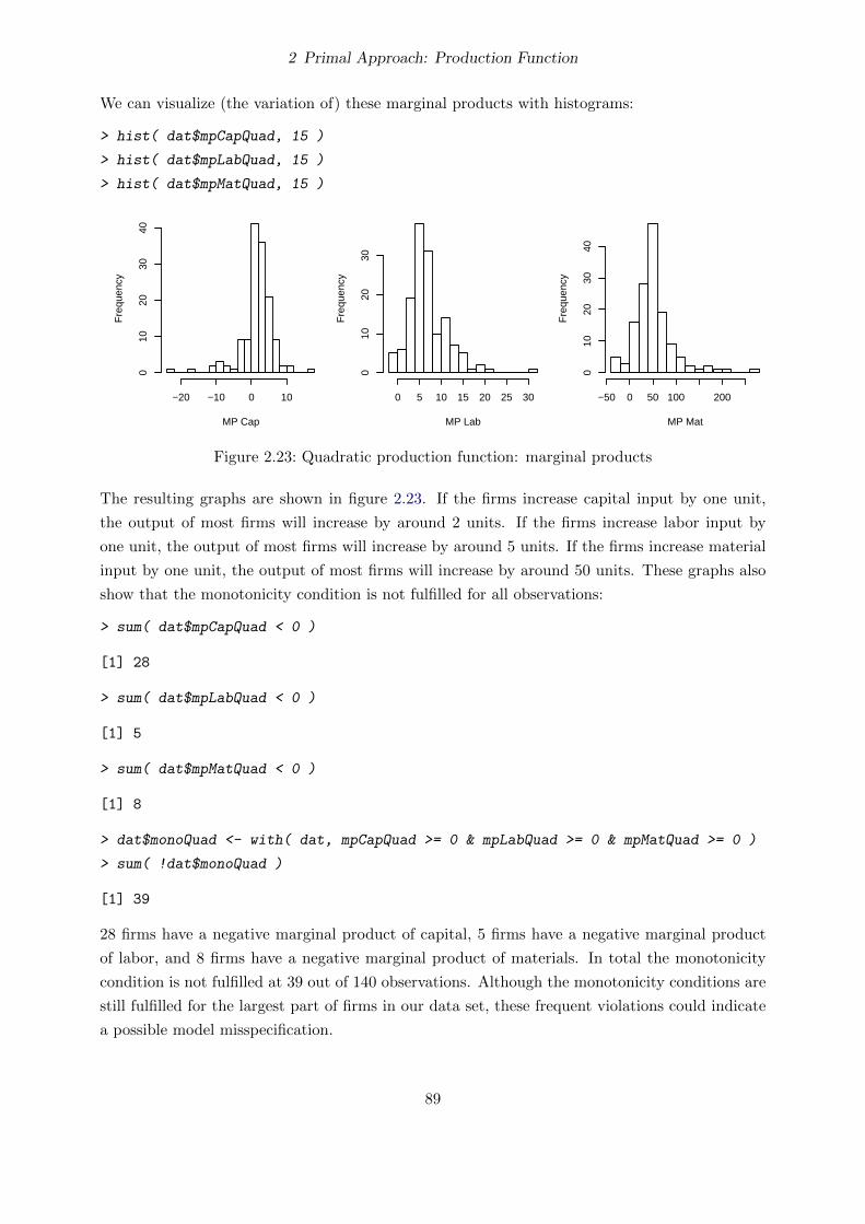
2 Primal Approach: Production Function
We can visualize (the variation of) these marginal products with histograms:
> hist( dat$mpCapQuad, 15 )
> hist( dat$mpLabQuad, 15 )
> hist( dat$mpMatQuad, 15 )
MP Cap
Fre
quen
cy
−20 −10 0 10
010
2030
40
MP Lab
Fre
quen
cy
0 5 10 15 20 25 30
010
2030
MP Mat
Fre
quen
cy
−50 0 50 100 200
010
2030
40
Figure 2.23: Quadratic production function: marginal products
The resulting graphs are shown in figure 2.23. If the firms increase capital input by one unit,
the output of most firms will increase by around 2 units. If the firms increase labor input by
one unit, the output of most firms will increase by around 5 units. If the firms increase material
input by one unit, the output of most firms will increase by around 50 units. These graphs also
show that the monotonicity condition is not fulfilled for all observations:
> sum( dat$mpCapQuad < 0 )
[1] 28
> sum( dat$mpLabQuad < 0 )
[1] 5
> sum( dat$mpMatQuad < 0 )
[1] 8
> dat$monoQuad <- with( dat, mpCapQuad >= 0 & mpLabQuad >= 0 & mpMatQuad >= 0 )
> sum( !dat$monoQuad )
[1] 39
28 firms have a negative marginal product of capital, 5 firms have a negative marginal product
of labor, and 8 firms have a negative marginal product of materials. In total the monotonicity
condition is not fulfilled at 39 out of 140 observations. Although the monotonicity conditions are
still fulfilled for the largest part of firms in our data set, these frequent violations could indicate
a possible model misspecification.
89

2 Primal Approach: Production Function
2.5.6 Output Elasticities
We can obtain output elasticities based on the quadratic production function by the standard
formula for output elasticities:
εi = MPixiy
(2.102)
As explained in section 2.4.11.1, we will use the predicted output quantities rather than the
observed output quantities. We can calculate the output elasticities with:
> dat$eCapQuad <- with( dat, mpCapQuad * qCap / qOutQuad )
> dat$eLabQuad <- with( dat, mpLabQuad * qLab / qOutQuad )
> dat$eMatQuad <- with( dat, mpMatQuad * qMat / qOutQuad )
We can visualize (the variation of) these output elasticities with histograms:
> hist( dat$eCapQuad, 15 )
> hist( dat$eLabQuad, 15 )
> hist( dat$eMatQuad, 15 )
eCap
Fre
quen
cy
−0.4 0.0 0.4 0.8
010
2030
4050
eLab
Fre
quen
cy
−0.5 0.0 0.5 1.0 1.5 2.0 2.5
010
2030
eMat
Fre
quen
cy
−1.5 −0.5 0.5 1.0 1.5
010
2030
4050
60
Figure 2.24: Quadratic production function: output elasticities
The resulting graphs are shown in figure 2.24. If the firms increase capital input by one percent,
the output of most firms will increase by around 0.05 percent. If the firms increase labor input
by one percent, the output of most firms will increase by around 0.7 percent. If the firms increase
material input by one percent, the output of most firms will increase by around 0.5 percent.
2.5.7 Elasticity of Scale
The elasticity of scale can—as always—be calculated as the sum of all output elasticities.
> dat$eScaleQuad <- dat$eCapQuad + dat$eLabQuad +
+ dat$eMatQuad
The (variation of the) elasticities of scale can be visualized with a histogram.
90

2 Primal Approach: Production Function
> hist( dat$eScaleQuad, 30 )
> hist( dat$eScaleQuad[ dat$monoQuad ], 30 )
eScaleQuad
Fre
quen
cy
0.8 1.0 1.2 1.4 1.6
05
1525
eScaleQuad[ monoQuad ]
Fre
quen
cy
1.1 1.3 1.5 1.7
02
46
812
Figure 2.25: Quadratic production function: elasticities of scale
The resulting graphs are shown in figure 2.25. Only a very few firms (4 out of 140) experience
decreasing returns to scale. If we only consider the observations where all monotonicity conditions
are fulfilled, our results suggest that all firms have increasing returns to scale. Most firms have an
elasticity of scale around 1.3. Hence, if these firms increase all input quantities by one percent,
the output of most firms will increase by around 1.3 percent. These elasticities of scale are much
more realistic than the elasticities of scale based on the linear production function.
Information on the optimal firm size can be obtained by analyzing the interrelationship between
firm size and the elasticity of scale, where we can either use the observed output or the quantity
index of the inputs as proxies of the firm size:
> plot( dat$qOut, dat$eScaleQuad, log = "x" )
> abline( 1, 0 )
> plot( dat$X, dat$eScaleQuad, log = "x" )
> abline( 1, 0 )
> plot( dat$qOut[ dat$monoQuad ], dat$eScaleQuad[ dat$monoQuad ], log = "x" )
> plot( dat$X[ dat$monoQuad ], dat$eScaleQuad[ dat$monoQuad ], log = "x" )
The resulting graphs are shown in figure 2.26. They all indicate that there are increasing returns
to scale for all firm sizes in the sample. Hence, all firms in the sample would gain from increasing
their size and the optimal firm size seems to be larger than the largest firm in the sample.
2.5.8 Marginal Rates of Technical Substitution
We can calculate the marginal rates of technical substitution (MRTS) based on our estimated
quadratic production function by following commands:
91

2 Primal Approach: Production Function
●
●●
●
●●
●●
●
●
● ●● ●
●
●
●
●
●
●●
●
●
●
●
●●
●
●
●●
●
●
●
●
●
●
●●
●
●
●
●
●●
●●
●
●
●
●
●
●
●
●
●
●
●
●
●
●
●
●
●
●
●
●●
● ●●
●●
●
●● ●●
●
●
●
●
●
●●●●●
●
●
●●
●
●
● ●
● ●
●
●●
●
●●
●●
●
●
●●●
● ●●●
●
●
●
●●
●
●
●
●
●
●
●●
●
●●
●
●
●
●
●●
●
●
●
1e+05 5e+05 2e+06 1e+07
0.8
1.0
1.2
1.4
1.6
observed output
eSca
leQ
uad
●
●●
●
●●
●●
●
●
● ●● ●
●
●
●
●
●
●●
●
●
●
●
●●
●
●
●●
●
●
●
●
●
●
●●
●
●
●
●
●●
●●
●
●
●
●
●
●
●
●
●
●
●
●
●
●
●
●
●
●
●
●●
● ●●●
●
●
●●●●
●
●
●
●
●
●● ●●●
●
●
●●
●
●
● ●
● ●
●
●●
●
● ●
●●
●
●
●●●
●●●●
●
●
●
●●
●
●
●
●
●
●
●●
●
● ●
●
●
●
●
●●
●
●
●
0.5 1.0 2.0 5.0
0.8
1.0
1.2
1.4
1.6
quantity index of inputs
eSca
leQ
uad
●
●
●
●
●
●● ●
●
●
●●
●
●
●
●
●●●
●
●
●
●
●
●
●
●
●
●
●
●
●
●
●
●
●
●
●
●
●
●
●
● ●
●
●
● ●
●
●
●●
●
●
●
● ●●
●
●
●
●
●●
●●●
●
●●
●
● ●
●
●● ●
●
● ●
●●
●
●
●
●●
●
●
●
●●
●●
●
●
●
●
●
●
●
1e+05 5e+05 2e+06 5e+06
1.1
1.3
1.5
1.7
observed output
eSca
leQ
uad[
mon
oQua
d ]
●
●
●
●
●
●● ●
●
●
● ●
●
●
●
●
●●
●
●
●
●
●
●
●
●
●
●
●
●
●
●
●
●
●
●
●
●
●
●
●
●
● ●
●
●
● ●
●
●
●●
●
●
●
●●●
●
●
●
●
●●
●●●
●
●●
●
● ●
●
●●●
●
●●
●●
●
●
●
●●
●
●
●
●●
● ●
●
●
●
●
●
●
●
0.5 1.0 2.01.
11.
31.
51.
7
quantity index of inputs
eSca
leQ
uad[
mon
oQua
d ]
Figure 2.26: Quadratic production function: elasticities of scale at different firm sizes
> dat$mrtsCapLabQuad <- with( dat, - mpLabQuad / mpCapQuad )
> dat$mrtsLabCapQuad <- with( dat, - mpCapQuad / mpLabQuad )
> dat$mrtsCapMatQuad <- with( dat, - mpMatQuad / mpCapQuad )
> dat$mrtsMatCapQuad <- with( dat, - mpCapQuad / mpMatQuad )
> dat$mrtsLabMatQuad <- with( dat, - mpMatQuad / mpLabQuad )
> dat$mrtsMatLabQuad <- with( dat, - mpLabQuad / mpMatQuad )
As the marginal rates of technical substitution (MRTS) are meaningless if the monotonicity
condition is not fulfilled, we visualize (the variation of) these MRTSs only for the observations,
where the monotonicity condition is fulfilled:
> hist( dat$mrtsCapLabQuad[ dat$monoQuad ], 30 )
> hist( dat$mrtsLabCapQuad[ dat$monoQuad ], 30 )
> hist( dat$mrtsCapMatQuad[ dat$monoQuad ], 30 )
> hist( dat$mrtsMatCapQuad[ dat$monoQuad ], 30 )
> hist( dat$mrtsLabMatQuad[ dat$monoQuad ], 30 )
> hist( dat$mrtsMatLabQuad[ dat$monoQuad ], 30 )
The resulting graphs are shown in figure 2.27. As some outliers hide the variation of the majority
of the RMRTS, we use function colMedians (package miscTools) to show the median values of
the MRTS:
92

2 Primal Approach: Production Function
mrtsCapLabQuad
Fre
quen
cy
−60 −40 −20 0
010
2030
40
mrtsLabCapQuad
Fre
quen
cy
−15 −10 −5 0
010
2030
4050
mrtsCapMatQuad
Fre
quen
cy
−1000 −600 −200 0
020
4060
80
mrtsMatCapQuad
Fre
quen
cy
−6 −5 −4 −3 −2 −1 0
020
4060
80
mrtsLabMatQuad
Fre
quen
cy
−60 −40 −20 0
05
1015
mrtsMatLabQuad
Fre
quen
cy
−3 −2 −1 0
010
2030
Figure 2.27: Quadratic production function: marginal rates of technical substitution (RMRTS)
> colMedians( subset( dat, monoQuad,
+ c( "mrtsCapLabQuad", "mrtsLabCapQuad", "mrtsCapMatQuad",
+ "mrtsMatCapQuad", "mrtsLabMatQuad", "mrtsMatLabQuad" ) ) )
mrtsCapLabQuad mrtsLabCapQuad mrtsCapMatQuad mrtsMatCapQuad mrtsLabMatQuad
-2.23505371 -0.44741654 -14.19802214 -0.07043235 -7.86423950
mrtsMatLabQuad
-0.12715788
Given that the median marginal rate of technical substitution between capital and labor is -2.24,
a typical firm that reduces the use of labor by one unit, has to use around 2.24 additional units
of capital in order to produce the same amount of output as before. Alternatively, the typical
firm can replace one unit of labor by using 0.13 additional units of materials.
2.5.9 Relative Marginal Rates of Technical Substitution
As we do not have a practical interpretation of the units of measurement of the input quantities,
the relative marginal rates of technical substitution (RMRTS) are practically more meaningful
than the MRTS. The following commands calculate the RMRTS:
93

2 Primal Approach: Production Function
> dat$rmrtsCapLabQuad <- with( dat, - eLabQuad / eCapQuad )
> dat$rmrtsLabCapQuad <- with( dat, - eCapQuad / eLabQuad )
> dat$rmrtsCapMatQuad <- with( dat, - eMatQuad / eCapQuad )
> dat$rmrtsMatCapQuad <- with( dat, - eCapQuad / eMatQuad )
> dat$rmrtsLabMatQuad <- with( dat, - eMatQuad / eLabQuad )
> dat$rmrtsMatLabQuad <- with( dat, - eLabQuad / eMatQuad )
As the (relative) marginal rates of technical substitution are meaningless if the monotonicity
condition is not fulfilled, we visualize (the variation of) these RMRTSs only for the observations,
where the monotonicity condition is fulfilled:
> hist( dat$rmrtsCapLabQuad[ dat$monoQuad ], 30 )
> hist( dat$rmrtsLabCapQuad[ dat$monoQuad ], 30 )
> hist( dat$rmrtsCapMatQuad[ dat$monoQuad ], 30 )
> hist( dat$rmrtsMatCapQuad[ dat$monoQuad ], 30 )
> hist( dat$rmrtsLabMatQuad[ dat$monoQuad ], 30 )
> hist( dat$rmrtsMatLabQuad[ dat$monoQuad ], 30 )
rmrtsCapLabQuad
Fre
quen
cy
−800 −600 −400 −200 0
020
4060
80
rmrtsLabCapQuad
Fre
quen
cy
−20 −15 −10 −5 0
020
4060
80
rmrtsCapMatQuad
Fre
quen
cy
−700 −500 −300 −100
020
4060
80
rmrtsMatCapQuad
Fre
quen
cy
−40 −30 −20 −10 0
020
4060
80
rmrtsLabMatQuad
Fre
quen
cy
−6 −4 −2 0
05
1015
20
rmrtsMatLabQuad
Fre
quen
cy
−15 −10 −5 0
05
1015
2025
3035
Figure 2.28: Quadratic production function: relative marginal rates of technical substitution(RMRTS)
The resulting graphs are shown in figure 2.28. As some outliers hide the variation of the majority
of the RMRTS, we use function colMedians (package miscTools) to show the median values of
94

2 Primal Approach: Production Function
the RMRTS:
> colMedians( subset( dat, monoQuad,
+ c( "rmrtsCapLabQuad", "rmrtsLabCapQuad", "rmrtsCapMatQuad",
+ "rmrtsMatCapQuad", "rmrtsLabMatQuad", "rmrtsMatLabQuad" ) ) )
rmrtsCapLabQuad rmrtsLabCapQuad rmrtsCapMatQuad rmrtsMatCapQuad rmrtsLabMatQuad
-5.5741780 -0.1793986 -4.2567577 -0.2349206 -0.7745132
rmrtsMatLabQuad
-1.2911336
Given that the median relative marginal rate of technical substitution between capital and labor
is -5.57, a typical firm that reduces the use of labor by one percent, has to use around 5.57 percent
more capital in order to produce the same amount of output as before. Alternatively, the typical
firm can replace one percent of labor by using 1.29 percent more materials.
2.5.10 Elasticities of Substitution
In the following, we only calculate the Allen elasticities of substitution. The calculation of
the direct elasticities of substitution and the Morishima elasticities of substitution requires only
minimal changes of the code. In order to check whether our calculations are correct, we can use
equation (2.15) to derive the following conditions:
∑i
xi MPi σij = 0 ∀ j (2.103)
In order to check this condition, we need to calculate not only (normal) elasticities of substitution
(σij ; i 6= j) but also economically not meaningful “elasticities of self-substitution” (σii):
> dat$esaCapLabQuad <- NA
> dat$esaCapMatQuad <- NA
> dat$esaLabMatQuad <- NA
> dat$esaCapCapQuad <- NA
> dat$esaLabLabQuad <- NA
> dat$esaMatMatQuad <- NA
> for( obs in 1:nrow( dat ) ) {
+ bhmLoop <- matrix( 0, nrow = 4, ncol = 4 )
+ bhmLoop[ 1, 2 ] <- bhmLoop[ 2, 1 ] <- dat$mpCapQuad[ obs ]
+ bhmLoop[ 1, 3 ] <- bhmLoop[ 3, 1 ] <- dat$mpLabQuad[ obs ]
+ bhmLoop[ 1, 4 ] <- bhmLoop[ 4, 1 ] <- dat$mpMatQuad[ obs ]
+ bhmLoop[ 2, 2 ] <- b11
+ bhmLoop[ 3, 3 ] <- b22
+ bhmLoop[ 4, 4 ] <- b33
95

2 Primal Approach: Production Function
+ bhmLoop[ 2, 3 ] <- bhmLoop[ 3, 2 ] <- b12
+ bhmLoop[ 2, 4 ] <- bhmLoop[ 4, 2 ] <- b13
+ bhmLoop[ 3, 4 ] <- bhmLoop[ 4, 3 ] <- b23
+ FCapLabLoop <- - det( bhmLoop[ -2, -3 ] )
+ FCapMatLoop <- det( bhmLoop[ -2, -4 ] )
+ FLabMatLoop <- - det( bhmLoop[ -3, -4 ] )
+ FCapCapLoop <- det( bhmLoop[ -2, -2 ] )
+ FLabLabLoop <- det( bhmLoop[ -3, -3 ] )
+ FMatMatLoop <- det( bhmLoop[ -4, -4 ] )
+ numerator <- with( dat[ obs, ],
+ qCap * mpCapQuad + qLab * mpLabQuad + qMat * mpMatQuad )
+ dat$esaCapLabQuad[ obs ] <- with( dat[obs,],
+ numerator / ( qCap * qLab ) * FCapLabLoop / det( bhmLoop ) )
+ dat$esaCapMatQuad[ obs ] <- with( dat[ obs, ],
+ numerator / ( qCap * qMat ) * FCapMatLoop / det( bhmLoop ) )
+ dat$esaLabMatQuad[ obs ] <- with( dat[ obs, ],
+ numerator / ( qLab * qMat ) * FLabMatLoop / det( bhmLoop ) )
+ dat$esaCapCapQuad[ obs ] <- with( dat[obs,],
+ numerator / ( qCap * qCap ) * FCapCapLoop / det( bhmLoop ) )
+ dat$esaLabLabQuad[ obs ] <- with( dat[ obs, ],
+ numerator / ( qLab * qLab ) * FLabLabLoop / det( bhmLoop ) )
+ dat$esaMatMatQuad[ obs ] <- with( dat[ obs, ],
+ numerator / ( qMat * qMat ) * FMatMatLoop / det( bhmLoop ) )
+ }
Before we take a look at and interpret the elasticities of substitution, we check whether the
conditions (2.103) are fulfilled:
> range( with( dat, qCap * mpCapQuad * esaCapCapQuad +
+ qLab * mpLabQuad * esaCapLabQuad + qMat * mpMatQuad * esaCapMatQuad ) )
[1] -1.117587e-08 2.533197e-07
> range( with( dat, qCap * mpCapQuad * esaCapLabQuad +
+ qLab * mpLabQuad * esaLabLabQuad + qMat * mpMatQuad * esaLabMatQuad ) )
[1] -5.587935e-09 1.862645e-09
> range( with( dat, qCap * mpCapQuad * esaCapMatQuad +
+ qLab * mpLabQuad * esaLabMatQuad + qMat * mpMatQuad * esaMatMatQuad ) )
[1] -9.313226e-09 3.725290e-09
96

2 Primal Approach: Production Function
The extremely small deviations from zero are most likely caused by rounding errors that are
unavoidable on digital computers. This test does not proof that all our calculations are done
correctly but if we had made a mistake, we would have discovered it with a very high probability.
Hence, we can be rather sure that our calculations are correct.
As the elasticities of substitution measure changes in the marginal rates of technical substitution
(MRTS) and the MRTS are meaningless if the monotonicity conditions are not fulfilled, also the
elasticities of substitution are meaningless if the monotonicity conditions are not fulfilled. Hence,
we visualize (the variation of) the Allen elasticities of substitution only for the observations,
where the monotonicity condition is fulfilled:
> hist( dat$esaCapLabQuad[ dat$monoQuad ], 30 )
> hist( dat$esaCapMatQuad[ dat$monoQuad ], 30 )
> hist( dat$esaLabMatQuad[ dat$monoQuad ], 30 )
esaCapLabQuad
Fre
quen
cy
−8 −6 −4 −2 0
010
2030
4050
esaCapMatQuad
Fre
quen
cy
−2 −1 0 1 2 3 4
05
1015
20
esaLabMatQuad
Fre
quen
cy
0.0 0.5 1.0 1.5 2.0 2.50
510
1520
25
Figure 2.29: Quadratic production function: elasticities of substitution
The resulting graphs are shown in figure 2.29. The estimated elasticities of substitution suggest
that capital and labor are always complements, labor and materials are always substitutes, and
capital and materials are partly complements and partly substitutes. The estimated elasticity
of substitution between labor and materials lies for the most firms between the value of the
Leontief production function (σ = 0) and the values of the Cobb-Douglas production function
(σ = 1). Hence, the substitutability between labor and materials seems to be between very low
and moderate. In fact, the elasticity of substitution between labor and materials is for a large
share of firms around 0.5. Hence, if labor is substituted for materials (or vice versa) so that the
MRTS between labor and materials increases (decreases) by one percent, the ratio between the
labor quantity and the quantity of materials increases (decreases) by 0.5 percent. If the firm is
minimizing costs and the price ratio between materials and labor increases by one percent, the
firm will substitute labor for materials so that ratio between the labor quantity and the quantity
of materials increases by 0.5 percent. Hence, the relative change of the quantity ratios is smaller
than the relative change of price ratios, which indicates a low substitutability between labor and
materials.
97
2 Primal Approach: Production Function
2.5.11 Quasiconcavity
We check whether our estimated quadratic production function is quasiconcave at each observa-
tion:
> dat$quasiConcQuad <- NA
> for( obs in 1:nrow( dat ) ) {
+ bhmLoop <- matrix( 0, nrow = 4, ncol = 4 )
+ bhmLoop[ 1, 2 ] <- bhmLoop[ 2, 1 ] <- dat$mpCapQuad[ obs ]
+ bhmLoop[ 1, 3 ] <- bhmLoop[ 3, 1 ] <- dat$mpLabQuad[ obs ]
+ bhmLoop[ 1, 4 ] <- bhmLoop[ 4, 1 ] <- dat$mpMatQuad[ obs ]
+ bhmLoop[ 2, 2 ] <- b11
+ bhmLoop[ 3, 3 ] <- b22
+ bhmLoop[ 4, 4 ] <- b33
+ bhmLoop[ 2, 3 ] <- bhmLoop[ 3, 2 ] <- b12
+ bhmLoop[ 2, 4 ] <- bhmLoop[ 4, 2 ] <- b13
+ bhmLoop[ 3, 4 ] <- bhmLoop[ 4, 3 ] <- b23
+ dat$quasiConcQuad[ obs ] <- det( bhmLoop[ 1:2, 1:2 ] ) < 0 &
+ det( bhmLoop[ 1:3, 1:3 ] ) > 0 & det( bhmLoop ) < 0
+ }
> sum( dat$quasiConcQuad )
[1] 0
Our estimated quadratic production function is quasiconcave at none of the 140 observations.
2.5.12 First-order conditions for profit maximisation
In this section, we will check to what extent the first-order conditions for profit maximization
(2.24) are fulfilled, i.e. to what extent the firms use the optimal input quantities. We do this by
comparing the marginal value products of the inputs with the corresponding input prices. We
can calculate the marginal value products by multiplying the marginal products by the output
price:
> dat$mvpCapQuad <- dat$pOut * dat$mpCapQuad
> dat$mvpLabQuad <- dat$pOut * dat$mpLabQuad
> dat$mvpMatQuad <- dat$pOut * dat$mpMatQuad
The command compPlot (package miscTools) can be used to compare the marginal value products
with the corresponding input prices. As the logarithm of a non-positive number is not defined,
we have to limit the comparisons on the logarithmic scale to observations with positive marginal
products:
98

2 Primal Approach: Production Function
> compPlot( dat$pCap, dat$mvpCapQuad )
> compPlot( dat$pLab, dat$mvpLabQuad )
> compPlot( dat$pMat, dat$mvpMatQuad )
> compPlot( dat$pCap[ dat$monoQuad ], dat$mvpCapQuad[ dat$monoQuad ], log = "xy" )
> compPlot( dat$pLab[ dat$monoQuad ], dat$mvpLabQuad[ dat$monoQuad ], log = "xy" )
> compPlot( dat$pMat[ dat$monoQuad ], dat$mvpMatQuad[ dat$monoQuad ], log = "xy" )
●●●●
●
●
●●●
●●●●●●
●
●●
●
●
●
●●
●●●●●●●●
●●●●●●●●●●●●
●●●●●
●
●●●●●●●●●
●●●●
●
●
●
●
●●
●
●
●●● ●●●●
●●●●
●
●●
●●●●●
●
●●
●
●
●
●
●
●● ●
●
●●●●
●●●●
●
●●●●●●●●●
●
●●●●
●
●●●
●
●●
●
●
●
●●
●
●●●
−60 −40 −20 0
−60
−40
−20
0
w Cap
MV
P C
ap
●
●●
●●
●
●
●
●
●
●
●●●
●
●
●
●
●●
●
●
●●
●●
●●●●●●
●
●●
●
●●
●
●
●
●●
●
●
●
●
●
●●●
●
●
●●
●
●
●●
●
●
●●●
●
●
●
●
●●
●
●
●
●●
●●
●
●●●
●
●
●●
●
●
●
●
●
●●
●
●
●
●
●
●
●
●
●
●
●
●●
●
●
●
●
●●
●
●●
●●
●
●●●
●
●
●●
●
●
●●
●
●
●
●
●●
●
●●●
●●
0 10 20 30 40
010
2030
40
w Lab
MV
P L
ab
●
●●●●
●
●
●●●
●
●
●
●
●
●
●
●
●
●
●
●●
●●●●●●●●●
●
●●
●
●●
●
●
●
●
●
●
●
●
●●●●●●●●●●●●●
●●
●●
●
●
●
●
●
●
●
●
●
●●●●●●●●●
●
●
●●
●●●
●
●
●●
●
●
●
●
●
●
●
●
●●
●
●
●
●
●
●
●
●
●●
●
●●
●●●
●●●●●
●
●
●
●●
●
●●
●
●
●
●●
●
●●
●
0 100 300 500
010
020
030
040
050
0
w Mat
MV
P M
at●●
●
●●
●●●
●
●
●
●
●
●
●
●
●
●
●
●
●●
●●
●
●
●●
●
●
●
●
●
●
●
●
●
●
●●
●●
●
●
●
●
●
●
●
●
●●●
●
●
●
●
●
●
●
●
●●
●●●
●
●
● ●
●
●
●●
●
●●
●
●●
● ●
●
●
●
●
●
●●
●
●
●
●●
●●
●
●
●
●
●
0.1 0.5 2.0 5.0
0.1
0.5
2.0
5.0
w Cap
MV
P C
ap
●
●●
●
●
●●●
●
●●
●
●
●
●
●●●
●
●
●
●●
●
●
●
●●
●
●
●
●
●
●
●
●
●
●
●
●
●
●
●●●
●
●
●
●
●
●
●
●
●
●
●
●
●
●●●
●
●
●
●
●
●
●
●
●
●
●
●
●
●●
●●
●
●
●
●
●
●●
●
●
●●
●
●
●●
●
●
●
●●●
● ●
0.5 1.0 2.0 5.0 20.0
0.5
1.0
2.0
5.0
10.0
w Lab
MV
P L
ab
●
●
●
●●
●
●
●
●
●
●
●
●●
●
●
●
●
●
●
●
●●
●
●
●
●
●
●
●●
●
●
●
●●
●
●
●
●●●
●
●
●
●
●
●
●
●
●
●
●
●
●●
● ●
●●
●
●
●
●
●● ●
●
●
●
●
●
●●
●●●
●
●
●
●
●
●
●
●●
●
●
●
●
●
●
●
●
●
●●
●
● ●
●
5 10 20 50 100
510
2050
100
w Mat
MV
P M
at
Figure 2.30: Marginal value products and corresponding input prices
The resulting graphs are shown in figure 2.30. They indicate that the marginal value products of
most firms are higher than the corresponding input prices. This indicates that most firms could
increase their profit by using more of all inputs. Given that the estimated quadratic function
shows that (almost) all firms operate under increasing returns to scale, it is not surprising that
most firms would gain from increasing all input quantities. Therefore, the question arises why the
firms in the sample did not do this. This questions has already been addressed in section 2.3.10.
2.5.13 First-order conditions for cost minimization
As the marginal rates of technical substitution differ between observations for the three other
functional forms, we use scatter plots for visualizing the comparison of the input price ratios
99

2 Primal Approach: Production Function
with the negative inverse marginal rates of technical substitution. As the marginal rates of
technical substitution are meaningless if the monotonicity condition is not fulfilled, we limit the
comparisons to the observations, where all monotonicity conditions are fulfilled:
> compPlot( ( dat$pCap / dat$pLab )[ dat$monoQuad ],
+ - dat$mrtsLabCapQuad[ dat$monoQuad ] )
> compPlot( ( dat$pCap / dat$pMat )[ dat$monoQuad ],
+ - dat$mrtsMatCapQuad[ dat$monoQuad ] )
> compPlot( ( dat$pLab / dat$pMat )[ dat$monoQuad ],
+ - dat$mrtsMatLabQuad[ dat$monoQuad ] )
> compPlot( ( dat$pCap / dat$pLab )[ dat$monoQuad ],
+ - dat$mrtsLabCapQuad[ dat$monoQuad ], log = "xy" )
> compPlot( ( dat$pCap / dat$pMat )[ dat$monoQuad ],
+ - dat$mrtsMatCapQuad[ dat$monoQuad ], log = "xy" )
> compPlot( ( dat$pLab / dat$pMat )[ dat$monoQuad ],
+ - dat$mrtsMatLabQuad[ dat$monoQuad ], log = "xy" )
●●●●
●
● ●● ●
●
●
●
●●●● ●●●
●●● ●●
●
●●●●
●●
●
●
●●●●●●
●
●●●
●
●
●●●●
●
●●
● ●●
●●
●
●●●
●
●●●●●
●●●
● ●●
●●●●●●●
●
●
●●
●
●
● ●● ●●
●
●
●
●
●
●
●
●●●
0 5 10 15
05
1015
w Cap / w Lab
− M
RT
S L
ab C
ap
●●●
●●●●●●
●
●●●●●●●● ●●●
● ●●●●●●●●●●
●●●●●●
●●●●●●●●●●
●
●
●●● ●●● ●●●●
●●
●
●●●●●
●
●●●
● ●●●●●●●
●●
●●●●●●●
●●●●●●● ●●●●●
0 1 2 3 4 5 6
01
23
45
6
w Cap / w Mat
− M
RT
S M
at C
ap
●
●
●
●●
●
●●
●
●
●●
●
●
●●●●
●●
●
●●●●●●●●●●
●
●●●●●
●
●●●
●●●
●●●●
●
●
●●●●●●●●●●
●
●
●
●
●●●
●
●
●
●
●
●
●
●●●●
●
●
●
●●●●●●●
●
●●●●●●●●
●●●
●
0 1 2 3
01
23
w Lab / w Mat
− M
RT
S M
at L
ab
●
●
●
●
●
●●●
●
●
●
●
●●
●
●●
●
●
●
●●
●
●
●
●
●●●
●●
●
●
●●
●●
●
●
●
●
● ●
●
●
●
●●●
●
●
●
●
●
●
●
●
●
●
●
●
●
●
●
●●●
●
●
●
●
●
●
●
●
●
●●
●●
●
●
●
●
●
●
●
●
●
●
●
●
●
●
●
●
●
●
●●
●
0.02 0.10 0.50 2.00 10.00
0.02
0.10
0.50
2.00
10.0
0
w Cap / w Lab
− M
RT
S L
ab C
ap
●
●●
●●
●
●
●
●
●
●
●●
●
●
●
●
●
●
●
●
●●
●
●
●
●
●●
●
●
●
●
●
●
●
●
●
●
●●●
●●
●
●
●●
●
●
●
●
●
●
●
●
●
●
●
●
●
●
●
●
● ●
●●
●
●
●
●
●●
●●●
●
●
●
●
●
●
●
●
●
● ●
●
●
●
●
●
●
●
●
●
●
●
●
●
0.001 0.010 0.100 1.000
0.00
10.
010
0.10
01.
000
w Cap / w Mat
− M
RT
S M
at C
ap
●
●
●
●
●
●
●
●
●
●
●
●
●
●
●
●
●
●
●
●
●
●●
●
●
●
●
●
●●
●
●
●
●
●
●
●
●
●
●
●
●
●
●
●
●
●
●
●
●
● ●
● ●●
● ●
●
●●
●
●
●
●
●
●
●
●
●
●
●
●
●
●
●●
●
●
●
●
●
●
●
●
●
●
●
●
●
●●●
●
●●
●
●
●
●
●
●
0.02 0.10 0.50 2.00
0.02
0.05
0.20
0.50
2.00
w Lab / w Mat
− M
RT
S M
at L
ab
Figure 2.31: First-order conditions for costs minimization
The resulting graphs are shown in figure 2.31.
100

2 Primal Approach: Production Function
Furthermore, we use histograms to visualize the (absolute and relative) differences between the
input price ratios and the corresponding negative inverse marginal rates of technical substitution:
> hist( ( - dat$mrtsLabCapQuad - dat$pCap / dat$pLab )[ dat$monoQuad ] )
> hist( ( - dat$mrtsMatCapQuad - dat$pCap / dat$pMat )[ dat$monoQuad ] )
> hist( ( - dat$mrtsMatLabQuad - dat$pLab / dat$pMat )[ dat$monoQuad ] )
> hist( log( - dat$mrtsLabCapQuad / ( dat$pCap / dat$pLab ) )[ dat$monoQuad ] )
> hist( log( - dat$mrtsMatCapQuad / (dat$pCap / dat$pMat ) )[ dat$monoQuad ] )
> hist( log( - dat$mrtsMatLabQuad / (dat$pLab / dat$pMat ) )[ dat$monoQuad ] )
− MrtsLabCap − wCap / wLab
Fre
quen
cy
−5 0 5 10 15
010
2030
4050
6070
− MrtsMatCap − wCap / wMat
Fre
quen
cy
0 2 4 6
020
4060
− MrtsMatLab − wLab / wMatF
requ
ency
0 1 2 3 4
010
2030
4050
60
log(−MrtsLabCap / (wCap / wLab))
Fre
quen
cy
−6 −4 −2 0 2 4
05
1015
2025
30
log(−MrtsMatCap / (wCap / wMat))
Fre
quen
cy
−6 −4 −2 0 2 4 6
05
1015
2025
log(−MrtsMatLab / (Lab / wMat))
Fre
quen
cy
−3 −2 −1 0 1 2 3 4
010
2030
40
Figure 2.32: First-order conditions for costs minimization
The resulting graphs are shown in figure 2.32. The left graphs in figures 2.31 and 2.32 show that
the ratio between the capital price and the labor price is larger than the absolute value of the
marginal rate of technical substitution between labor and capital for a majority of the firms in
the sample:wcapwlab
> −MRTSlab,cap = MPcapMPlab
(2.104)
Hence, these firms can get closer to the minimum of their production costs by substituting labor
for capital, because this will decrease the marginal product of labor and increase the marginal
101
2 Primal Approach: Production Function
product of capital so that the absolute value of the MRTS between labor and capital increases
and gets closer to the corresponding input price ratio. Similarly, the graphs in the middle column
indicate that a majority of the firms should substitute materials for capital and the graphs on
the right indicate that a little more than half of the firms should substitute materials for labor.
Hence, the majority of the firms could reduce production costs particularly by using less capital
and using more labor or more materials. 5
2.6 Translog Production Function
2.6.1 Specification
The Translog function is a more flexible extension of the Cobb-Douglas function as the quadratic
function is a more flexible extension of the linear function. Hence, the Translog function can be
seen as a combination of the Cobb-Douglas function and the quadratic function. The Translog
production function has following specification:
ln y = α0 +∑i
αi ln xi + 12∑i
∑j
αij ln xi ln xj (2.105)
with αij = αji.
2.6.2 Estimation
We can estimate this Translog production function with the command
> prodTL <- lm( log( qOut ) ~ log( qCap ) + log( qLab ) + log( qMat )
+ + I( 0.5 * log( qCap )^2 ) + I( 0.5 * log( qLab )^2 )
+ + I( 0.5 * log( qMat )^2 ) + I( log( qCap ) * log( qLab ) )
+ + I( log( qCap ) * log( qMat ) ) + I( log( qLab ) * log( qMat ) ),
+ data = dat )
> summary( prodTL )
Call:
lm(formula = log(qOut) ~ log(qCap) + log(qLab) + log(qMat) +
I(0.5 * log(qCap)^2) + I(0.5 * log(qLab)^2) + I(0.5 * log(qMat)^2) +
I(log(qCap) * log(qLab)) + I(log(qCap) * log(qMat)) + I(log(qLab) *
log(qMat)), data = dat)
Residuals:
Min 1Q Median 3Q Max
-1.68015 -0.36688 0.05389 0.44125 1.26560
5 This generally confirms the results of the Cobb-Douglas production function.
102

2 Primal Approach: Production Function
Coefficients:
Estimate Std. Error t value Pr(>|t|)
(Intercept) -4.14581 21.35945 -0.194 0.8464
log(qCap) -2.30683 2.28829 -1.008 0.3153
log(qLab) 1.99328 4.56624 0.437 0.6632
log(qMat) 2.23170 3.76334 0.593 0.5542
I(0.5 * log(qCap)^2) -0.02573 0.20834 -0.124 0.9019
I(0.5 * log(qLab)^2) -1.16364 0.67943 -1.713 0.0892 .
I(0.5 * log(qMat)^2) -0.50368 0.43498 -1.158 0.2490
I(log(qCap) * log(qLab)) 0.56194 0.29120 1.930 0.0558 .
I(log(qCap) * log(qMat)) -0.40996 0.23534 -1.742 0.0839 .
I(log(qLab) * log(qMat)) 0.65793 0.42750 1.539 0.1262
---
Signif. codes: 0 ‘***’ 0.001 ‘**’ 0.01 ‘*’ 0.05 ‘.’ 0.1 ‘ ’ 1
Residual standard error: 0.6412 on 130 degrees of freedom
Multiple R-squared: 0.6296, Adjusted R-squared: 0.6039
F-statistic: 24.55 on 9 and 130 DF, p-value: < 2.2e-16
None of the estimated coefficients is statistically significantly different from zero at the 5% sig-
nificance level and only three coefficients are statistically significant at the 10% level. As the
Cobb-Douglas production function is “nested” in the Translog production function, we can apply
a “Wald test” or “likelihood ratio test” to check whether the Cobb-Douglas production function is
rejected in favor of the Translog production function. This can be done by the functions waldtest
and lrtest (package lmtest):
> waldtest( prodCD, prodTL )
Wald test
Model 1: log(qOut) ~ log(qCap) + log(qLab) + log(qMat)
Model 2: log(qOut) ~ log(qCap) + log(qLab) + log(qMat) + I(0.5 * log(qCap)^2) +
I(0.5 * log(qLab)^2) + I(0.5 * log(qMat)^2) + I(log(qCap) *
log(qLab)) + I(log(qCap) * log(qMat)) + I(log(qLab) * log(qMat))
Res.Df Df F Pr(>F)
1 136
2 130 6 2.062 0.06202 .
---
Signif. codes: 0 ‘***’ 0.001 ‘**’ 0.01 ‘*’ 0.05 ‘.’ 0.1 ‘ ’ 1
> lrtest( prodCD, prodTL )
103

2 Primal Approach: Production Function
Likelihood ratio test
Model 1: log(qOut) ~ log(qCap) + log(qLab) + log(qMat)
Model 2: log(qOut) ~ log(qCap) + log(qLab) + log(qMat) + I(0.5 * log(qCap)^2) +
I(0.5 * log(qLab)^2) + I(0.5 * log(qMat)^2) + I(log(qCap) *
log(qLab)) + I(log(qCap) * log(qMat)) + I(log(qLab) * log(qMat))
#Df LogLik Df Chisq Pr(>Chisq)
1 5 -137.61
2 11 -131.25 6 12.727 0.04757 *
---
Signif. codes: 0 ‘***’ 0.001 ‘**’ 0.01 ‘*’ 0.05 ‘.’ 0.1 ‘ ’ 1
At the 5% significance level, the Cobb-Douglas production function is accepted by the Wald test
but rejected in favor of the Translog production function by the likelihood ratio test. In order
to reduce the chance of using a too restrictive functional form, we proceed with the Translog
production function.
2.6.3 Properties
We cannot see from the estimated coefficients whether the monotonicity condition is fulfilled. The
Translog production function cannot be globally monotone, because there will be always a set of
input quantities that result in negative marginal products.6 The Translog function would only be
globally monotone, if all first-order coefficients are positive and all second-order coefficients are
zero, which is equivalent to a Cobb-Douglas function. We will check the monotonicity condition
at each observation in section 2.6.5.
All Translog production functions fulfill the weak and the strong essentiality assumption, be-
cause as soon as a single input quantity approaches zero, the right-hand side of equation (2.105)
approaches minus infinity (if monotonicity is fulfilled), and thus, the output quantity y = exp(ln y)approaches zero. Hence, if a data set includes observations with a positive output quantity but
at least one input quantity that is zero, strict essentiality cannot be fulfilled in the underlying
true production technology so that the Translog production function is not a suitable functional
form for analyzing this data set.
The input requirement sets derived from Translog production functions are always closed and
non-empty. The Translog production function always returns finite, real, non-negative, and single
values as long as all input quantities are strictly positive. All Translog production functions are
continuous and twice-continuously differentiable.
6 Please note that ln xj is a large negative number if xj is a very small positive number.
104

2 Primal Approach: Production Function
2.6.4 Predicted Output Quantities
As before, we can easily obtain the predicted output quantities with the fitted method. As we
used the logarithmic output quantity as dependent variable in our estimated model, we must use
the exponential function to obtain the output quantities measured in levels:
> dat$qOutTL <- exp( fitted( prodTL ) )
Now, we can evaluate the “fit” of the model by comparing the observed with the fitted output
quantities:
> compPlot( dat$qOut, dat$qOutTL )
> compPlot( dat$qOut, dat$qOutTL, log = "xy" )
●●
●●●
●
●●●●●
●
●●
●
●
●
●
●●
●●
●●●
●●
●
● ●●●●●●
●●● ●●●●● ●● ●●
●●●●●●●
●●●●●
●
●●
●
●●
●●
●
●●
●● ●●●
●●
●●●●
●
●
●
●
●
●● ●
●
●●
●
●
●
●
● ●● ●
●●
●● ●● ●
●
●●
●●●●●●
●● ●
●
●● ●
●●
●●●
●
●●
●
●
●
●●
●
●
●
●
0.0e+00 1.0e+07 2.0e+07
0.0e
+00
1.0e
+07
2.0e
+07
observed
fitte
d
●●
●
●●
●
●● ●
●
●
●
●
●
●
●
●
●
●
●
●
●
●●
●
●
●
●
●
●●
● ●
●●
●
●
●
●
●
●●
●
●●●
●
●●
●●●
●●
● ●●
●●
●
●
●
●
●
●
●●
●
●●
●● ●
●
●
●
●
●
●
●●
●
●
●
●
●
●
●
●
●
●●
●
●
●
●
●●
●●
●●
●
● ●● ●
●
●●
●●
●●
●
●
●●
●
●
●
● ●
●●
●
●
●
●
●●
●
●
●
●
●
●
●
●
●
1e+05 5e+05 5e+06
1e+
055e
+05
2e+
061e
+07
observed
fitte
d
Figure 2.33: Translog production function: fit of the model
The resulting graphs are shown in figure 2.33. While the graph in the left panel uses a linear
scale for the axes, the graph in the right panel uses a logarithmic scale for both axes. Hence,
the deviations from the 45°-line illustrate the absolute deviations in the left panel and the rel-
ative deviations in the right panel. The fit of the model looks rather okay, but there are some
observations, at which the predicted output quantity is not very close to the observed output
quantity.
2.6.5 Output Elasticities
The output elasticities calculated from a Translog production function are:
εi = ∂ ln y∂ ln xi
= αi +∑j
αij ln xj (2.106)
We can simplify the code for computing these output elasticities by using short names for the
coefficients:
105

2 Primal Approach: Production Function
> a1 <- coef( prodTL )[ "log(qCap)" ]
> a2 <- coef( prodTL )[ "log(qLab)" ]
> a3 <- coef( prodTL )[ "log(qMat)" ]
> a11 <- coef( prodTL )[ "I(0.5 * log(qCap)^2)" ]
> a22 <- coef( prodTL )[ "I(0.5 * log(qLab)^2)" ]
> a33 <- coef( prodTL )[ "I(0.5 * log(qMat)^2)" ]
> a12 <- a21 <- coef( prodTL )[ "I(log(qCap) * log(qLab))" ]
> a13 <- a31 <- coef( prodTL )[ "I(log(qCap) * log(qMat))" ]
> a23 <- a32 <- coef( prodTL )[ "I(log(qLab) * log(qMat))" ]
Now, we can use the following commands to calculate the output elasticities in R:
> dat$eCapTL <- with( dat,
+ a1 + a11 * log(qCap) + a12 * log(qLab) + a13 * log(qMat) )
> dat$eLabTL <- with( dat,
+ a2 + a21 * log(qCap) + a22 * log(qLab) + a23 * log(qMat) )
> dat$eMatTL <- with( dat,
+ a3 + a31 * log(qCap) + a32 * log(qLab) + a33 * log(qMat) )
We can visualize (the variation of) these output elasticities with histograms:
> hist( dat$eCapTL, 15 )
> hist( dat$eLabTL, 15 )
> hist( dat$eMatTL, 15 )
eCap
Fre
quen
cy
−0.4 0.0 0.4 0.8
05
1015
2025
eLab
Fre
quen
cy
−1.0 0.0 0.5 1.0 1.5 2.0
05
1015
2025
eMat
Fre
quen
cy
0.0 0.5 1.0 1.5 2.0
010
2030
Figure 2.34: Translog production function: output elasticities
The resulting graphs are shown in figure 2.34. If the firms increase capital input by one percent,
the output of most firms will increase by around 0.2 percent. If the firms increase labor input by
one percent, the output of most firms will increase by around 0.5 percent. If the firms increase
material input by one percent, the output of most firms will increase by around 0.7 percent.
These graphs also show that the monotonicity condition is not fulfilled for all observations:
106

2 Primal Approach: Production Function
> sum( dat$eCapTL < 0 )
[1] 32
> sum( dat$eLabTL < 0 )
[1] 14
> sum( dat$eMatTL < 0 )
[1] 8
> dat$monoTL <- with( dat, eCapTL >= 0 & eLabTL >= 0 & eMatTL >= 0 )
> sum( !dat$monoTL )
[1] 48
32 firms have a negative output elasticity of capital, 14 firms have a negative output elasticity
of labor, and 8 firms have a negative output elasticity of materials. In total the monotonicity
condition is not fulfilled at 48 out of 140 observations. Although the monotonicity conditions
are fulfilled for a large part of firms in our data set, these frequent violations indicate a possible
model misspecification.
2.6.6 Marginal Products
The first derivatives (marginal products) of the Translog production function with respect to the
input quantities are:
MPi = ∂y
∂xi= y
xi
∂ ln y∂ ln xi
= y
xi
αi +∑j
αij ln xj
(2.107)
We can calculate the marginal products based on the output elasticities that we have calculated
above. As argued in section 2.4.11.1, we use the predicted output quantities in this calculation:
> dat$mpCapTL <- with( dat, eCapTL * qOutTL / qCap )
> dat$mpLabTL <- with( dat, eLabTL * qOutTL / qLab )
> dat$mpMatTL <- with( dat, eMatTL * qOutTL / qMat )
We can visualize (the variation of) these marginal products with histograms:
> hist( dat$mpCapTL, 15 )
> hist( dat$mpLabTL, 15 )
> hist( dat$mpMatTL, 15 )
The resulting graphs are shown in figure 2.35. If the firms increase capital input by one unit,
the output of most firms will increase by around 4 units. If the firms increase labor input by
one unit, the output of most firms will increase by around 4 units. If the firms increase material
input by one unit, the output of most firms will increase by around 70 units.
107
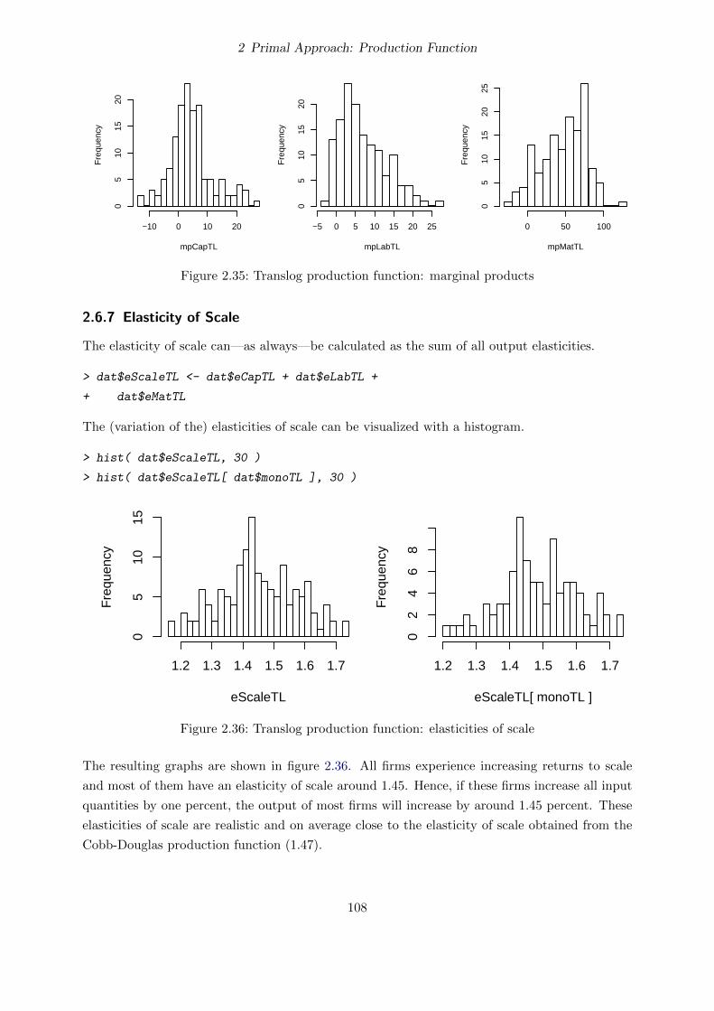
2 Primal Approach: Production Function
mpCapTL
Fre
quen
cy
−10 0 10 20
05
1015
20
mpLabTL
Fre
quen
cy
−5 0 5 10 15 20 25
05
1015
20
mpMatTL
Fre
quen
cy
0 50 100
05
1015
2025
Figure 2.35: Translog production function: marginal products
2.6.7 Elasticity of Scale
The elasticity of scale can—as always—be calculated as the sum of all output elasticities.
> dat$eScaleTL <- dat$eCapTL + dat$eLabTL +
+ dat$eMatTL
The (variation of the) elasticities of scale can be visualized with a histogram.
> hist( dat$eScaleTL, 30 )
> hist( dat$eScaleTL[ dat$monoTL ], 30 )
eScaleTL
Fre
quen
cy
1.2 1.3 1.4 1.5 1.6 1.7
05
1015
eScaleTL[ monoTL ]
Fre
quen
cy
1.2 1.3 1.4 1.5 1.6 1.7
02
46
8
Figure 2.36: Translog production function: elasticities of scale
The resulting graphs are shown in figure 2.36. All firms experience increasing returns to scale
and most of them have an elasticity of scale around 1.45. Hence, if these firms increase all input
quantities by one percent, the output of most firms will increase by around 1.45 percent. These
elasticities of scale are realistic and on average close to the elasticity of scale obtained from the
Cobb-Douglas production function (1.47).
108

2 Primal Approach: Production Function
Information on the optimal firm size can be obtained by analyzing the relationship between
firm size and the elasticity of scale. We can either use the observed or the predicted output:
> plot( dat$qOut, dat$eScaleTL, log = "x" )
> plot( dat$X, dat$eScaleTL, log = "x" )
> plot( dat$qOut[ dat$monoTL ], dat$eScaleTL[ dat$monoTL ], log = "x" )
> plot( dat$X[ dat$monoTL ], dat$eScaleTL[ dat$monoTL ], log = "x" )
●
●
●●
●
●●
●
●
●
●
●
●
●
●
●
●
●
●
●
●
●
●
●
●
●
●
●● ●●
●
●●
●
●
●
●
●
●
●
●●
●
●
●
●
●
●
●●
●
●
●●
●
●
●●
●●
●
●
●
●
●
●
● ●
●
●
●
●
●
●
●
●
●
●●
●
●
●
●●
●●
●
●
●●
●
●
●
●
●
●
●
●
●
●
●
●
●
●
●
●
●
●
●
●
●
●●
●
●
●
●●
●
●
●
●
●●
●
●
●
●
●●
●
●
●
●
● ●
●
●
●
1e+05 5e+05 2e+06 1e+07
1.2
1.4
1.6
observed output
eSca
leT
L
●
●
●●
●
●●
●
●
●
●
●
●
●
●
●
●
●
●
●
●
●
●
●
●
●
●
●● ● ●
●
●●
●
●
●
●
●
●
●
●●
●
●
●
●
●
●
●●
●
●
●●
●
●
●●
●●
●
●
●
●
●
●
● ●
●
●
●
●
●
●
●
●
●
●●
●
●
●
●●
●●
●
●
●●
●
●
●
●
●
●
●
●
●
●
●
●
●
●
●
●
●
●
●
●
●
●●
●
●
●
●●
●
●
●
●
●●
●
●
●
●
●●
●
●
●
●
● ●
●
●
●
0.5 1.0 2.0 5.0
1.2
1.4
1.6
quantity index of inputs
eSca
leT
L
●
●
●
●
●
●
●
●●
● ●
●
●
●
●
●
●● ●●●
●
●
●
●●
●
●●
●
●●
●
●
●
●
●●
●
●
●
●
●
●
●
●
●
●
●
●
●
●
●●
●
●●
●
●
●
●
●
●
●
●
●
●
●
●
●
●
●
●
●
●
●
●●
●
●
●
●
●
●
●●
●
●
●
●
●
●
1e+05 5e+05 2e+06 1e+07
1.2
1.3
1.4
1.5
1.6
1.7
observed output
eSca
leT
L[ m
onoT
L ]
●
●
●
●
●
●
●
●●
●●
●
●
●
●
●
●● ● ●●
●
●
●
●●
●
●●
●
●●
●
●
●
●
●●
●
●
●
●
●
●
●
●
●
●
●
●
●
●
●●
●
●●
●
●
●
●
●
●
●
●
●
●
●
●
●
●
●
●
●
●
●
●●
●
●
●
●
●
●
●●
●
●
●
●
●
●
0.5 1.0 2.0 5.0
1.2
1.3
1.4
1.5
1.6
1.7
quantity index of inputs
eSca
leT
L[ m
onoT
L ]
Figure 2.37: Translog production function: elasticities of scale at different firm sizes
The resulting graphs are shown in figure 2.37. Both of them indicate that the elasticity of scale
slightly decreases with firm size but there are considerable increasing returns to scale even for
the largest firms in the sample. Hence, all firms in the sample would gain from increasing their
size and the optimal firm size seems to be larger than the largest firm in the sample.
2.6.8 Marginal Rates of Technical Substitution
We can calculate the marginal rates of technical substitution (MRTS) based on our estimated
Translog production function by following commands:
> dat$mrtsCapLabTL <- with( dat, - mpLabTL / mpCapTL )
> dat$mrtsLabCapTL <- with( dat, - mpCapTL / mpLabTL )
> dat$mrtsCapMatTL <- with( dat, - mpMatTL / mpCapTL )
109

2 Primal Approach: Production Function
> dat$mrtsMatCapTL <- with( dat, - mpCapTL / mpMatTL )
> dat$mrtsLabMatTL <- with( dat, - mpMatTL / mpLabTL )
> dat$mrtsMatLabTL <- with( dat, - mpLabTL / mpMatTL )
As the marginal rates of technical substitution are meaningless if the monotonicity condition is
not fulfilled, we visualize (the variation of) these MRTS only for the observations, where the
monotonicity condition is fulfilled:
> hist( dat$mrtsCapLabTL[ dat$monoTL ], 30 )
> hist( dat$mrtsLabCapTL[ dat$monoTL ], 30 )
> hist( dat$mrtsCapMatTL[ dat$monoTL ], 30 )
> hist( dat$mrtsMatCapTL[ dat$monoTL ], 30 )
> hist( dat$mrtsLabMatTL[ dat$monoTL ], 30 )
> hist( dat$mrtsMatLabTL[ dat$monoTL ], 30 )
mrtsCapLabTL
Fre
quen
cy
−150 −100 −50 0
020
4060
mrtsLabCapTL
Fre
quen
cy
−60 −40 −20 0
010
2030
4050
60
mrtsCapMatTL
Fre
quen
cy
−800 −600 −400 −200 00
1020
3040
5060
70
mrtsMatCapTL
Fre
quen
cy
−0.6 −0.4 −0.2 0.0
05
1015
mrtsLabMatTL
Fre
quen
cy
−1200 −800 −400 0
020
4060
80
mrtsMatLabTL
Fre
quen
cy
−4 −3 −2 −1 0
010
2030
4050
Figure 2.38: Translog production function: marginal rates of technical substitution (MRTS)
The resulting graphs are shown in figure 2.39. As some outliers hide the variation of the majority
of the MRTS, we use function colMedians (package miscTools) to show the median values of the
MRTS:
> colMedians( subset( dat, monoTL,
+ c( "mrtsCapLabTL", "mrtsLabCapTL", "mrtsCapMatTL",
+ "mrtsMatCapTL", "mrtsLabMatTL", "mrtsMatLabTL" ) ) )
110

2 Primal Approach: Production Function
mrtsCapLabTL mrtsLabCapTL mrtsCapMatTL mrtsMatCapTL mrtsLabMatTL mrtsMatLabTL
-0.83929283 -1.19196521 -12.72554396 -0.07858435 -12.79850828 -0.07813810
Given that the median marginal rate of technical substitution between capital and labor is -0.84,
a typical firm that reduces the use of labor by one unit, has to use around 0.84 additional units
of capital in order to produce the same amount of output as before. Alternatively, the typical
firm can replace one unit of labor by using 0.08 additional units of materials.
2.6.9 Relative Marginal Rates of Technical Substitution
As we do not have a practical interpretation of the units of measurement of the input quantities,
the relative marginal rates of technical substitution (RMRTS) are practically more meaningful
than the MRTS. The following commands calculate the RMRTS:
> dat$rmrtsCapLabTL <- with( dat, - eLabTL / eCapTL )
> dat$rmrtsLabCapTL <- with( dat, - eCapTL / eLabTL )
> dat$rmrtsCapMatTL <- with( dat, - eMatTL / eCapTL )
> dat$rmrtsMatCapTL <- with( dat, - eCapTL / eMatTL )
> dat$rmrtsLabMatTL <- with( dat, - eMatTL / eLabTL )
> dat$rmrtsMatLabTL <- with( dat, - eLabTL / eMatTL )
As the (relative) marginal rates of technical substitution are meaningless if the monotonicity
condition is not fulfilled, we visualize (the variation of) these RMRTS only for the observations,
where the monotonicity condition is fulfilled:
> hist( dat$rmrtsCapLabTL[ dat$monoTL ], 30 )
> hist( dat$rmrtsLabCapTL[ dat$monoTL ], 30 )
> hist( dat$rmrtsCapMatTL[ dat$monoTL ], 30 )
> hist( dat$rmrtsMatCapTL[ dat$monoTL ], 30 )
> hist( dat$rmrtsLabMatTL[ dat$monoTL ], 30 )
> hist( dat$rmrtsMatLabTL[ dat$monoTL ], 30 )
The resulting graphs are shown in figure 2.39. As some outliers hide the variation of the majority
of the RMRTS, we use function colMedians (package miscTools) to show the median values of
the RMRTS:
> colMedians( subset( dat, monoTL,
+ c( "rmrtsCapLabTL", "rmrtsLabCapTL", "rmrtsCapMatTL",
+ "rmrtsMatCapTL", "rmrtsLabMatTL", "rmrtsMatLabTL" ) ) )
rmrtsCapLabTL rmrtsLabCapTL rmrtsCapMatTL rmrtsMatCapTL rmrtsLabMatTL
-2.8357239 -0.3539150 -3.0064237 -0.3331325 -1.3444115
rmrtsMatLabTL
-0.7439008
111

2 Primal Approach: Production Function
rmrtsCapLabTL
Fre
quen
cy
−500 −300 −100 0
020
4060
80
rmrtsLabCapTL
Fre
quen
cy
−25 −20 −15 −10 −5 0
020
4060
rmrtsCapMatTL
Fre
quen
cy
−400 −300 −200 −100 0
020
4060
80
rmrtsMatCapTL
Fre
quen
cy
−3.0 −2.0 −1.0 0.0
05
1015
20
rmrtsLabMatTL
Fre
quen
cy
−50 −40 −30 −20 −10 0
010
2030
4050
60
rmrtsMatLabTL
Fre
quen
cy
−35 −25 −15 −5 0
010
2030
4050
Figure 2.39: Translog production function: relative marginal rates of technical substitution(RMRTS)
112

2 Primal Approach: Production Function
Given that the median relative marginal rate of technical substitution between capital and labor
is -2.84, a typical firm that reduces the use of labor by one percent, has to use around 2.84 percent
more capital in order to produce the same amount of output as before. Alternatively, the typical
firm can replace one percent of labor by using 0.74 percent more materials.
2.6.10 Second partial derivatives
In order to compute the elasticities of substitution, we need obtain the second derivatives of the
Translog function. We can calculate them as derivatives of the first derivatives of the Translog
function:
∂2y
∂xi∂xj=∂
(∂y
∂xi
)∂xj
=∂
((αi +
∑k αik ln xk)
y
xi
)∂xj
(2.108)
= αijxj
y
xi+ αi +
∑k αik ln xkxi
∂y
∂xj− δij
(αi +
∑k
αik ln xk
)y
x2i
(2.109)
= αij y
xi xj+ αi +
∑k αik ln xkxi
(αj +
∑k
αjk ln xk
)y
xj− δij
(αi +
∑k
αik ln xk
)y
x2i
(2.110)
= αij y
xi xj+ εi εj y
xi xj− δij
εi y
x2i
(2.111)
= y
xi xj(αij + εi εj − δijεi) , (2.112)
where δij is (again) Kronecker’s delta (2.66). Alternatively, the second derivatives of the Translog
function can be expressed based on the marginal products (instead of the output elasticities):
∂2y
∂xi∂xj= αij y
xi xj+ MPi MPj
y− δij
MPixi
(2.113)
Now, we can calculate the second derivatives for each observation in our data set:
> dat$fCapCapTL <- with( dat,
+ qOutTL / qCap^2 * ( a11 + eCapTL^2 - eCapTL ) )
> dat$fLabLabTL <- with( dat,
+ qOutTL / qLab^2 * ( a22 + eLabTL^2 - eLabTL ) )
> dat$fMatMatTL <- with( dat,
+ qOutTL / qMat^2 * ( a33 + eMatTL^2 - eMatTL ) )
> dat$fCapLabTL <- with( dat,
+ qOutTL / ( qCap * qLab ) * ( a12 + eCapTL * eLabTL ) )
> dat$fCapMatTL <- with( dat,
+ qOutTL / ( qCap * qMat ) * ( a13 + eCapTL * eMatTL ) )
> dat$fLabMatTL <- with( dat,
113

2 Primal Approach: Production Function
+ qOutTL / ( qLab * qMat ) * ( a23 + eLabTL * eMatTL ) )
2.6.11 Elasticities of Substitution
As for the quadratic production function, we only calculate the Allen elasticities of substitution.
The calculation of the direct elasticities of substitution and the Morishima elasticities of substi-
tution requires only minimal changes of the code. In order to check whether our calculations are
correct, we will—as before—check if the conditions (2.103) are fulfilled. In order to check these
conditions, we need to calculate not only (normal) elasticities of substitution (σij ; i 6= j) but also
economically not meaningful “elasticities of self-substitution” (σii):
> dat$esaCapLabTL <- NA
> dat$esaCapMatTL <- NA
> dat$esaLabMatTL <- NA
> dat$esaCapCapTL <- NA
> dat$esaLabLabTL <- NA
> dat$esaMatMatTL <- NA
> for( obs in 1:nrow( dat ) ) {
+ bhmLoop <- matrix( 0, nrow = 4, ncol = 4 )
+ bhmLoop[ 1, 2 ] <- bhmLoop[ 2, 1 ] <- dat$mpCapTL[ obs ]
+ bhmLoop[ 1, 3 ] <- bhmLoop[ 3, 1 ] <- dat$mpLabTL[ obs ]
+ bhmLoop[ 1, 4 ] <- bhmLoop[ 4, 1 ] <- dat$mpMatTL[ obs ]
+ bhmLoop[ 2, 2 ] <- dat$fCapCapTL[ obs ]
+ bhmLoop[ 3, 3 ] <- dat$fLabLabTL[ obs ]
+ bhmLoop[ 4, 4 ] <- dat$fMatMatTL[ obs ]
+ bhmLoop[ 2, 3 ] <- bhmLoop[ 3, 2 ] <- dat$fCapLabTL[ obs ]
+ bhmLoop[ 2, 4 ] <- bhmLoop[ 4, 2 ] <- dat$fCapMatTL[ obs ]
+ bhmLoop[ 3, 4 ] <- bhmLoop[ 4, 3 ] <- dat$fLabMatTL[ obs ]
+ FCapLabLoop <- - det( bhmLoop[ -2, -3 ] )
+ FCapMatLoop <- det( bhmLoop[ -2, -4 ] )
+ FLabMatLoop <- - det( bhmLoop[ -3, -4 ] )
+ FCapCapLoop <- det( bhmLoop[ -2, -2 ] )
+ FLabLabLoop <- det( bhmLoop[ -3, -3 ] )
+ FMatMatLoop <- det( bhmLoop[ -4, -4 ] )
+ numerator <- with( dat[ obs, ],
+ qCap * mpCapTL + qLab * mpLabTL + qMat * mpMatTL )
+ dat$esaCapLabTL[ obs ] <- with( dat[obs,],
+ numerator / ( qCap * qLab ) * FCapLabLoop / det( bhmLoop ) )
+ dat$esaCapMatTL[ obs ] <- with( dat[ obs, ],
+ numerator / ( qCap * qMat ) * FCapMatLoop / det( bhmLoop ) )
+ dat$esaLabMatTL[ obs ] <- with( dat[ obs, ],
114

2 Primal Approach: Production Function
+ numerator / ( qLab * qMat ) * FLabMatLoop / det( bhmLoop ) )
+ dat$esaCapCapTL[ obs ] <- with( dat[obs,],
+ numerator / ( qCap * qCap ) * FCapCapLoop / det( bhmLoop ) )
+ dat$esaLabLabTL[ obs ] <- with( dat[ obs, ],
+ numerator / ( qLab * qLab ) * FLabLabLoop / det( bhmLoop ) )
+ dat$esaMatMatTL[ obs ] <- with( dat[ obs, ],
+ numerator / ( qMat * qMat ) * FMatMatLoop / det( bhmLoop ) )
+ }
Before we take a look at and interpret the elasticities of substitution, we check whether the
conditions (2.103) are fulfilled:
> range( with( dat, qCap * mpCapTL * esaCapCapTL +
+ qLab * mpLabTL * esaCapLabTL + qMat * mpMatTL * esaCapMatTL ) )
[1] -3.337860e-06 6.705523e-08
> range( with( dat, qCap * mpCapTL * esaCapLabTL +
+ qLab * mpLabTL * esaLabLabTL + qMat * mpMatTL * esaLabMatTL ) )
[1] -1.862645e-08 2.235174e-08
> range( with( dat, qCap * mpCapTL * esaCapMatTL +
+ qLab * mpLabTL * esaLabMatTL + qMat * mpMatTL * esaMatMatTL ) )
[1] -9.536743e-07 2.793968e-08
The extremely small deviations from zero are most likely caused by rounding errors that are
unavoidable on digital computers. This test does not proof that all of our calculations are done
correctly but if we had made a mistake, we probably would have discovered it. Hence, we can be
rather sure that our calculations are correct.
As the elasticities of substitution measure changes in the marginal rates of technical substitution
(MRTS) and the MRTS are meaningless if the monotonicity conditions are not fulfilled, also the
elasticities of substitution are meaningless if the monotonicity conditions are not fulfilled. Hence,
we visualize (the variation of) the Allen elasticities of substitution only for the observations,
where the monotonicity condition is fulfilled:
> hist( dat$esaCapLabTL[ dat$monoTL ], 30 )
> hist( dat$esaCapMatTL[ dat$monoTL ], 30 )
> hist( dat$esaLabMatTL[ dat$monoTL ], 30 )
> hist( dat$esaCapLabTL[ dat$monoTL & abs( dat$esaCapLabTL ) < 10 ], 30 )
> hist( dat$esaCapMatTL[ dat$monoTL & abs( dat$esaCapMatTL ) < 10 ], 30 )
> hist( dat$esaLabMatTL[ dat$monoTL & abs( dat$esaLabMatTL ) < 10 ], 30 )
115

2 Primal Approach: Production Function
esaCapLabTL
Fre
quen
cy
−400 −200 0
010
2030
4050
esaCapMatTL
Fre
quen
cy
0 500 1000 1500
010
2030
4050
esaLabMatTL
Fre
quen
cy
0 50 100 150
010
2030
4050
abs( esaCapLabTL ) < 10
Fre
quen
cy
−10 −5 0 5
05
1015
abs( esaCapMatTL ) < 10
Fre
quen
cy
−10 −5 0 5
02
46
810
12
abs( esaLabMatTL ) < 10
Fre
quen
cy
−4 −2 0 2 4 6 8
05
1015
2025
Figure 2.40: Translog production function: elasticities of substitution
The resulting graphs are shown in figure 2.40. The estimated elasticities of substitution between
capital and labor suggest that capital and labor are substitutes for almost half of the firms but
complements for the majority of firms. In contrast, capital and materials as well as labor and
materials are substitutes for the majority of firms. As some outliers hide the variation of the
majority of the elasticities of substitution, we use function colMedians (package miscTools) to
obtain the median values of the Allen elasticities of substitution:
> colMedians( subset( dat, monoTL,
+ c( "esaCapLabTL", "esaCapMatTL", "esaLabMatTL" ) ) )
esaCapLabTL esaCapMatTL esaLabMatTL
-0.2130532 2.5436068 0.4193423
The median elasticity of substitution between labor and materials (0.42) lies between the elasticity
of substitution of the Leontief production function (σ = 0) and the elasticity of substitution of
the Cobb-Douglas production function (σ = 1). Hence, the substitutability between labor and
materials seems to be rather low. A typical firm who substitutes materials for labor (or vice versa)
so that the MRTS between materials and labor increases (decreases) by one percent, has increased
(decreased) the ratio between the quantity of materials and the labor quantity by 0.42 percent. If
the firm is maximizing profit or minimizing costs and the price ratio between labor and materials
116

2 Primal Approach: Production Function
increases by one percent, the firm will substitute materials for labor so that the ratio between
the quantity of materials and the labor quantity increases by 0.42 percent. Hence, the relative
change of the quantity ratio is smaller than the relative change of price ratio, which indicates a low
substitutability between labor and materials. In contrast, the median elasticity of substitution
between capital and materials is larger than one (2.54), which indicates that it is much easier to
substitute between capital and materials.
2.6.12 Quasiconcavity
We check whether our estimated Translog production function is quasiconcave at each observa-
tion:
> dat$quasiConcTL <- NA
> for( obs in 1:nrow( dat ) ) {
+ bhmLoop <- matrix( 0, nrow = 4, ncol = 4 )
+ bhmLoop[ 1, 2 ] <- bhmLoop[ 2, 1 ] <- dat$mpCapTL[ obs ]
+ bhmLoop[ 1, 3 ] <- bhmLoop[ 3, 1 ] <- dat$mpLabTL[ obs ]
+ bhmLoop[ 1, 4 ] <- bhmLoop[ 4, 1 ] <- dat$mpMatTL[ obs ]
+ bhmLoop[ 2, 2 ] <- dat$fCapCapTL[ obs ]
+ bhmLoop[ 3, 3 ] <- dat$fLabLabTL[ obs ]
+ bhmLoop[ 4, 4 ] <- dat$fMatMatTL[ obs ]
+ bhmLoop[ 2, 3 ] <- bhmLoop[ 3, 2 ] <- dat$fCapLabTL[ obs ]
+ bhmLoop[ 2, 4 ] <- bhmLoop[ 4, 2 ] <- dat$fCapMatTL[ obs ]
+ bhmLoop[ 3, 4 ] <- bhmLoop[ 4, 3 ] <- dat$fLabMatTL[ obs ]
+ dat$quasiConcTL[ obs ] <- det( bhmLoop[ 1:2, 1:2 ] ) < 0 &
+ det( bhmLoop[ 1:3, 1:3 ] ) > 0 & det( bhmLoop ) < 0
+ }
> sum( dat$quasiConcTL )
[1] 63
Our estimated Translog production function is quasiconcave at 63 of the 140 observations.
2.6.13 First-order conditions for profit maximisation
In this section, we will check to what extent the first-order conditions for profit maximisation
(2.24) are fulfilled, i.e. to what extent the firms use the optimal input quantities. We do this by
comparing the marginal value products of the inputs with the corresponding input prices. We
can calculate the marginal value products by multiplying the marginal products by the output
price:
117

2 Primal Approach: Production Function
> dat$mvpCapTL <- dat$pOut * dat$mpCapTL
> dat$mvpLabTL <- dat$pOut * dat$mpLabTL
> dat$mvpMatTL <- dat$pOut * dat$mpMatTL
The command compPlot (package miscTools) can be used to compare the marginal value products
with the corresponding input prices. As the logarithm of a non-positive number is not defined,
we have to limit the comparisons on the logarithmic scale to observations with positve marginal
products:
> compPlot( dat$pCap, dat$mvpCapTL )
> compPlot( dat$pLab, dat$mvpLabTL )
> compPlot( dat$pMat, dat$mvpMatTL )
> compPlot( dat$pCap[ dat$monoTL ], dat$mvpCapTL[ dat$monoTL ], log = "xy" )
> compPlot( dat$pLab[ dat$monoTL ], dat$mvpLabTL[ dat$monoTL ], log = "xy" )
> compPlot( dat$pMat[ dat$monoTL ], dat$mvpMatTL[ dat$monoTL ], log = "xy" )
●
●●●●
●
●
●
●
●
●
●
●
●●
●
●
●●
●
●
●●
●●
●●●●●●
●●
●●●
●●
●
●
●
●
●●●●●●●●●●●
●
●●●●●●●
●●
●
●
●
●
●
●
●●●
●
●
●●●●●●●●
●●●●●●
●
●
●●
●
●
●
●
●
●●
●
●
●
●
●
●
●
●
●
●
●
●●
●
●●
●
●●●●
●
●●●
●
●
●●
●
●●
●
●
●
●●●
●
●
●
−40 0 20 40 60
−40
−20
020
4060
w Cap
MV
P C
ap
●
●
●
●●●
●
●
●
●
●
●
●
●
●
●
●
●●
●
●
●
●
●
●
●
●●
●●
●
●●
●●
●
●●●
●
●
●●
●
●●
●
●●
●●
●
●
●
●●
●
●●
●
●
●
●
●●
●
●
●
●
●
●●
●
●
●
●
●
●●●
●
●
●
●
●●●
●
●
●●●●
●
●
●
●
●●
●
●
●
●
●●●
●
●
●
●
●●
●
●
●
●
●●●
●
●
●●
●
●
●
●●
●
●●
●●●
●
●
●
●
●
●
−5 0 5 10 15 20 25 30
−5
05
1015
2025
30
w Lab
MV
P L
ab
●
●●
●●
●
●
●
●
●
●
●
●
●
●
●
●
●
●
●
●
●●
●●
●
●●
●●
●
●
●
●●
●
●●
●
●
●
●
●
●
●
●
●
●●
●
●
●
●
●
●
●●
●●
●
●
●
●
●
●
●
●
●
●
●
●
●
●
●
●
●●
●
●●
●●
●
●
●●
●
●●
●
●
●
●
●●
●●
●
●
●
●
●
●
●
●
●
●
●
●
●
●
●
●
●
●
●
●
●
●
●
●
●●
●
●●
●
●
●
●
●
●
●
●
●
●
●
●
●
●
0 50 100 150
050
100
150
w Mat
MV
P M
at
●
●
●
●●
●
●
●
●
●
●
●
●
●
●
●
●
●
●
●
●
●
●
●
●
●
●
●
●
●
●
●
●
●
●
●
●●
●
●
●
●
●
●
●
●
●
●
●●
●●● ●
●●●
●
●
●
●
●
●
●●
●
●
●
●
●
●
●
●
●
●
●
●
●
●
●●
● ●
●
●
●
●
●
●
●●
●
5e−02 5e−01 5e+00 5e+01
5e−
025e
−01
5e+
005e
+01
w Cap
MV
P C
ap
●
●
●
●
●
●
●
●
●
●
●
●
●●
●
●●
●●
●
●
●
●
●
●●
●
●
●
●
●
●
●
●
●
●
●
●
●
●
●●
●
●
●
●●
●
●
●
●
●
●
●
●
● ●
●
●●●
●
●
●●
●
●
●●
●
●
●
●
●●
●
●
●
●
●●●●
●
●●
●●●
●
●●
0.05 0.20 1.00 5.00 20.00
0.05
0.20
1.00
5.00
20.0
0
w Lab
MV
P L
ab
●
●
●
●
●
●
●
●
●
●
●
●
●
●
●
●●
● ●
●
●
●
●
●
●
●
●
●
●
●
●
●
●
●
●
●
●●
●
●
●
●
●
●
●
●
●
●
●
●●
●
●● ●
●
●
●●
●
●
●
●●
●
●
●
●
●
●
●
●
●
●
●
●●
●
●
●●●
●
●
●
●
●
●
●
●
●
●
5 10 20 50 100
510
2050
100
200
w Mat
MV
P M
at
Figure 2.41: Marginal value products and corresponding input prices
The resulting graphs are shown in figure 2.41. They indicate that the marginal value products of
most firms are higher than the corresponding input prices. This indicates that most firms could
118

2 Primal Approach: Production Function
increase their profit by using more of all inputs. Given that the estimated Translog function
shows that all firms operate under increasing returns to scale, it is not surprising that most firms
would gain from increasing all input quantities. Therefore, the question arises why the firms in
the sample did not do this. This questions has already been addressed in section 2.3.10.
2.6.14 First-order conditions for cost minimization
As the marginal rates of technical substitution differ between observations for the three other
functional forms, we use scatter plots for visualizing the comparison of the input price ratios
with the negative inverse marginal rates of technical substitution: As the marginal rates of
technical substitution are meaningless if the monotonicity condition is not fulfilled, we limit the
comparisons to the observations, where all monotonicity conditions are fulfilled:
> compPlot( ( dat$pCap / dat$pLab )[ dat$monoTL ],
+ - dat$mrtsLabCapTL[ dat$monoTL ] )
> compPlot( ( dat$pCap / dat$pMat )[ dat$monoTL ],
+ - dat$mrtsMatCapTL[ dat$monoTL ] )
> compPlot( ( dat$pLab / dat$pMat )[ dat$monoTL ],
+ - dat$mrtsMatLabTL[ dat$monoTL ] )
> compPlot( ( dat$pCap / dat$pLab )[ dat$monoTL ],
+ - dat$mrtsLabCapTL[ dat$monoTL ], log = "xy" )
> compPlot( ( dat$pCap / dat$pMat )[ dat$monoTL ],
+ - dat$mrtsMatCapTL[ dat$monoTL ], log = "xy" )
> compPlot( ( dat$pLab / dat$pMat )[ dat$monoTL ],
+ - dat$mrtsMatLabTL[ dat$monoTL ], log = "xy" )
The resulting graphs are shown in figure 2.42.
Furthermore, we use histograms to visualize the (absolute and relative) differences between the
input price ratios and the corresponding negative inverse marginal rates of technical substitution:
> hist( ( - dat$mrtsLabCapTL - dat$pCap / dat$pLab )[ dat$monoTL ] )
> hist( ( - dat$mrtsMatCapTL - dat$pCap / dat$pMat )[ dat$monoTL ] )
> hist( ( - dat$mrtsMatLabTL - dat$pLab / dat$pMat )[ dat$monoTL ] )
> hist( log( - dat$mrtsLabCapTL / ( dat$pCap / dat$pLab ) )[ dat$monoTL ] )
> hist( log( - dat$mrtsMatCapTL / ( dat$pCap / dat$pMat ) )[ dat$monoTL ] )
> hist( log( - dat$mrtsMatLabTL / ( dat$pLab / dat$pMat ) )[ dat$monoTL ] )
The resulting graphs are shown in figure 2.43. The graphs in the middle column of figures 2.42
and 2.43 show that the ratio between the capital price and the materials price is larger than the
absolute value of the marginal rate of technical substitution between materials and capital for a
majority of the firms in the sample:
wcapwmat
> −MRTSmat,cap = MPcapMPmat
(2.114)
119

2 Primal Approach: Production Function
●●
●●●●
●
●
●
●
●
●●●●●●●●●●●●●●●●●●●
●
●●●●
●
●●●●
●
●●●
●
●●
●●●●
●●
●
●●●●●●●
●
●●●
●
●
●
●
●
●
●
●●●
●
●
●●●●●●●
●●
●
●
●
●●●
0 20 40 60
020
4060
w Cap / w Lab
− M
RT
S L
ab C
ap
●
●
●
●●
●
●
●
●●
●●
●
● ●
●
●
●
●
●
●●
●
●●
●●
●
●●
●●
●
●●
●●●
●
●
●●
●
●
●
●●
●
●
●
●●
● ●●
●
●●
●
●
●
●
●
●
●
●
●
●
●
●●
●
●
●
●
●●
●
●
● ●●
●
●
●●
●
●
●
●
●●
0.0 0.1 0.2 0.3 0.4 0.5 0.6
0.0
0.1
0.2
0.3
0.4
0.5
0.6
w Cap / w Mat
− M
RT
S M
at C
ap
●●●●
●
●
●
●
●
●
●
●
●●●●●
●●●
●●●●●●●
●
●
●
●●
●
●●●
●●●●
●●
●●
●●
●
●●●●
●●●●
●
●
●●
●
●●
●
●●
●
●●●●●●
●
●●
●●●
●
●●●●●●
●
●●●●●●
0 1 2 3 4
01
23
4
w Lab / w Mat
− M
RT
S M
at L
ab
●
●
●
●
●
●
●
●
●
●
●
●
●
●
●
●
●●
●
●
●
●
●
●●
●●
●
●
●
●
●
●
●●
●
●
●●
●
●
●
●●
●
●
●
●
●
● ●
●●
●
●●●
●
●
●
●
●
●
●●
●
●
●
●
●
●
●
●
●
●
●
●
●
●
●
●●●
●
●
●
●
●
●
●
●
●
1e−02 1e+00 1e+02
1e−
021e
−01
1e+
001e
+01
1e+
02
w Cap / w Lab
− M
RT
S L
ab C
ap
●
●
●
●●
●
●
●
●●
●●
●
● ●
●
●
●
●
●
●●
●
●●
●●
●
●
●
●●
●
●●
●●
●
●
●
●●
●●
●
●
●
●
●
●
●
●
● ●
●
●
●●
●
●
●
●
●
●
●●
●
●
●
●●
●
●
●
●
●●●
●
●●
●
●
●
●●
●
●
●
●
●●
0.001 0.005 0.050 0.500
0.00
10.
005
0.02
00.
100
0.50
0
w Cap / w Mat
− M
RT
S M
at C
ap
●
●●
●
●
●
●
●
●
●
●
●
●
●
●
●●
●●
●
●
●●
●●
●●
●
●
●
●
●
●
●●
●
●
●
●
●
●
●
●●
●
●
●
●
●
●●
●
●
●
●
●
●
●
●
●
●
●
●
●
●
●
●
●
●
●
●
●
●
●
●
●
●
●
●
●●●
●●
●
●
●
●● ●
●
●
0.001 0.010 0.100 1.000
0.00
10.
010
0.10
01.
000
w Lab / w Mat
− M
RT
S M
at L
ab
Figure 2.42: First-order conditions for costs minimization
120
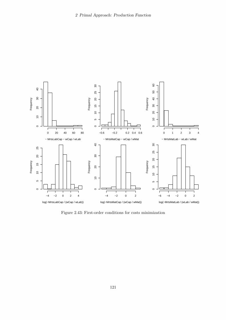
2 Primal Approach: Production Function
− MrtsLabCap − wCap / wLab
Fre
quen
cy
0 20 40 60 80
010
2030
40
− MrtsMatCap − wCap / wMat
Fre
quen
cy
−0.6 −0.2 0.2 0.4 0.6
05
1015
2025
30
− MrtsMatLab − wLab / wMat
Fre
quen
cy
0 1 2 3 4
010
2030
4050
60
log(−MrtsLabCap / (wCap / wLab))
Fre
quen
cy
−4 −2 0 2 4
05
1015
2025
log(−MrtsMatCap / (wCap / wMat))
Fre
quen
cy
−4 −2 0 2
010
2030
40
log(−MrtsMatLab / (wLab / wMat))
Fre
quen
cy
−6 −4 −2 0 2
05
1015
2025
30
Figure 2.43: First-order conditions for costs minimization
121

2 Primal Approach: Production Function
Hence, these firms can get closer to the minimum of their production costs by substituting
materials for capital, because this will decrease the marginal product of materials and increase
the marginal product of capital so that the absolute value of the MRTS between materials and
capital increases and gets closer to the corresponding input price ratio. The graphs on the left
indicate that approximately half of the firms should substitute labor for capital, while the other
half should substitute capital for labor. The graphs on the right indicate that a majority of
the firms should substitute materials for labor. Hence, the majority of the firms could reduce
production costs particularly by using more materials and using less labor or less capital but
there might be (legal) regulations that restrict the use of materials (e.g. fertilizers, pesticides).
2.6.15 Mean-scaled quantities
The Translog function is often estimated with mean-scaled variables. The following commands
create variables with mean-scaled output and input quantities:
> dat$qmOut <- with( dat, qOut / mean( qOut ) )
> dat$qmCap <- with( dat, qCap / mean( qCap ) )
> dat$qmLab <- with( dat, qLab / mean( qLab ) )
> dat$qmMat <- with( dat, qMat / mean( qMat ) )
This implies that the logarithms of the mean values of these variables are zero (except for negli-
gible very small rounding errors):
> log( colMeans( dat[ , c( "qmOut", "qmCap", "qmLab", "qmMat" ) ] ) )
qmOut qmCap qmLab qmMat
-1.110223e-16 -1.110223e-16 0.000000e+00 0.000000e+00
Please note that mean-scaling does not imply that the mean values of the logarithmic variables
are zero:
> colMeans( log( dat[ , c( "qmOut", "qmCap", "qmLab", "qmMat" ) ] ) )
qmOut qmCap qmLab qmMat
-0.4860021 -0.3212057 -0.1565112 -0.2128551
Now, we estimate the Translog production function with mean-scaled variables:
> prodTLm <- lm( log( qmOut ) ~ log( qmCap ) + log( qmLab ) + log( qmMat )
+ + I( 0.5 * log( qmCap )^2 ) + I( 0.5 * log( qmLab )^2 )
+ + I( 0.5 * log( qmMat )^2 ) + I( log( qmCap ) * log( qmLab ) )
+ + I( log( qmCap ) * log( qmMat ) ) + I( log( qmLab ) * log( qmMat ) ),
+ data = dat )
> summary( prodTLm )
122
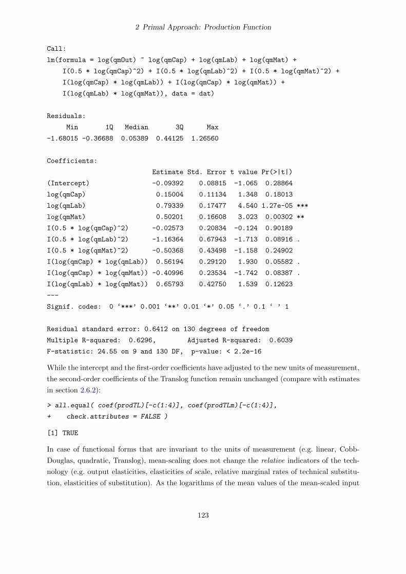
2 Primal Approach: Production Function
Call:
lm(formula = log(qmOut) ~ log(qmCap) + log(qmLab) + log(qmMat) +
I(0.5 * log(qmCap)^2) + I(0.5 * log(qmLab)^2) + I(0.5 * log(qmMat)^2) +
I(log(qmCap) * log(qmLab)) + I(log(qmCap) * log(qmMat)) +
I(log(qmLab) * log(qmMat)), data = dat)
Residuals:
Min 1Q Median 3Q Max
-1.68015 -0.36688 0.05389 0.44125 1.26560
Coefficients:
Estimate Std. Error t value Pr(>|t|)
(Intercept) -0.09392 0.08815 -1.065 0.28864
log(qmCap) 0.15004 0.11134 1.348 0.18013
log(qmLab) 0.79339 0.17477 4.540 1.27e-05 ***
log(qmMat) 0.50201 0.16608 3.023 0.00302 **
I(0.5 * log(qmCap)^2) -0.02573 0.20834 -0.124 0.90189
I(0.5 * log(qmLab)^2) -1.16364 0.67943 -1.713 0.08916 .
I(0.5 * log(qmMat)^2) -0.50368 0.43498 -1.158 0.24902
I(log(qmCap) * log(qmLab)) 0.56194 0.29120 1.930 0.05582 .
I(log(qmCap) * log(qmMat)) -0.40996 0.23534 -1.742 0.08387 .
I(log(qmLab) * log(qmMat)) 0.65793 0.42750 1.539 0.12623
---
Signif. codes: 0 ‘***’ 0.001 ‘**’ 0.01 ‘*’ 0.05 ‘.’ 0.1 ‘ ’ 1
Residual standard error: 0.6412 on 130 degrees of freedom
Multiple R-squared: 0.6296, Adjusted R-squared: 0.6039
F-statistic: 24.55 on 9 and 130 DF, p-value: < 2.2e-16
While the intercept and the first-order coefficients have adjusted to the new units of measurement,
the second-order coefficients of the Translog function remain unchanged (compare with estimates
in section 2.6.2):
> all.equal( coef(prodTL)[-c(1:4)], coef(prodTLm)[-c(1:4)],
+ check.attributes = FALSE )
[1] TRUE
In case of functional forms that are invariant to the units of measurement (e.g. linear, Cobb-
Douglas, quadratic, Translog), mean-scaling does not change the relative indicators of the tech-
nology (e.g. output elasticities, elasticities of scale, relative marginal rates of technical substitu-
tion, elasticities of substitution). As the logarithms of the mean values of the mean-scaled input
123

2 Primal Approach: Production Function
quantities are zero, the first-order coefficients are equal to the output elasticities at the sample
mean (see equation 2.106), i.e. the output elasticity of capital is 0.15, the output elasticity of
labor is 0.793, the output elasticity of materials is 0.502, and the elasticity of scale is 1.445 at
the sample mean.
2.7 Evaluation of Different Functional Forms
In this section, we will discuss the appropriateness of the four different functional forms for
analyzing the production technology in our data set. If one functional form is nested in another
functional form, we can use standard statistical tests to compare these functional forms. We have
done this already in section 2.5 (linear production function vs. quadratic production function)
and in section 2.6 (Cobb-Douglas production function vs. Translog production function). The
tests clearly reject the linear production function in favor of the quadratic production function
but it is less clear whether the Cobb-Douglas production function is rejected in favor of the
Translog production function.
It is much less straight-forward to compare non-nested models such as the quadratic and the
Translog production function.
2.7.1 Goodness of Fit
As the quadratic and the Translog models use different dependent variables (y vs. ln y), we cannot
simply compare the R2-values. However, we can calculate the hypothetical R2-value regarding y
for the Translog production function and compare it with the R2 value of the quadratic produc-
tion function. We can also calculate the hypothetical R2-value regarding ln y for the quadratic
production function and compare it with the R2 value of the Translog production function. We
can calculate the (hypothetical) R2 values with function rSquared (package miscTools). The first
argument of this function must be a vector of the observed dependent variable and the second ar-
gument must be a vector of the residuals. We start by extracting the R2 value from the quadratic
model and calculate the hypothetical R2-value regarding y for the Translog production function:
> summary(prodQuad)$r.squared
[1] 0.8448983
> rSquared( dat$qOut, dat$qOut - dat$qOutTL )
[,1]
[1,] 0.7696638
In this case, the R2 value regarding y is considerably higher for the quadratic function. Similarly,
we can extract the R2 value from the Translog model and calculate the hypothetical R2-value
regarding ln y for the quadratic production function:
124

2 Primal Approach: Production Function
> summary(prodTL)$r.squared
[1] 0.6295696
> rSquared( log( dat$qOut ), log( dat$qOut ) - log( dat$qOutQuad ) )
[,1]
[1,] 0.5481309
In contrast to the R2 value regarding y, the R2 value regarding ln y is considerably higher for
the Translog function. Hence, in our case, the R2 values do not help much to select the most
suitable functional form. We could base our comparison on the unadjusted R2 values, because
the quadratic and the Translog function have the same number of coefficients. If the compared
models have different numbers of coefficients, the comparison must be based on adjusted R2
values.
Furthermore, we can visually compare the fit of the two models by looking at figures 2.22
and 2.33. The quadratic production function is clearly over-predicting the output of small firms
so that small firms have rather large relative error terms. On the other hand, the Translog
production function has rather large absolute error terms for large firms. In total, it seems that
the fit of the Translog function is slightly better.
2.7.2 Theoretical Consistency
Furthermore, we can compare the theoretical consistency of the two models. The total number
of monotonicity violations of the quadratic production function and the Translog production
function can be obtained by
> with( dat, sum( eCapQuad < 0 ) + sum( eLabQuad < 0 ) + sum( eMatQuad < 0 ) )
[1] 41
> with( dat, sum( eCapTL < 0 ) + sum( eLabTL < 0 ) + sum( eMatTL < 0 ) )
[1] 54
Alternatively, we could look at the number of observations, at which the monotonicity condition
is violated:
> sum( !dat$monoQuad )
[1] 39
> sum( !dat$monoTL )
[1] 48
125

2 Primal Approach: Production Function
Both measures show that the monotonicity condition is more often violated in the Translog
function.
While the Translog production function always returns a positive output quantity (as long
as all input quantities are strictly positive), this is not necessarily the case for the quadratic
production function. However, we have checked this in section 2.5.6 and found that all output
quantities predicted by our quadratic production function are positive. Hence, the non-negativity
condition is fulfilled for both functional forms.
Quasiconcavity is fulfilled at 63 out of 140 observations for the Translog production function
but at no observation for the quadratic production function. However, quasiconcavity is mainly
assumed to simplify the (further) economic analysis (e.g. to obtain continuous input demand
and output supply functions) and there can be found good reasons for why the true production
technology is not quasiconcave (e.g. indivisibility of inputs).
2.7.3 Plausible Estimates
While the elasticities of scale of some observations were implausibly large when estimated with
the linear production function, no elasticities of scale estimated by the quadratic and Translog
production function are in the implausible range:
> sum( dat$eScaleQuad > 2 | dat$eScaleQuad < 0.5 )
[1] 0
> sum( dat$eScaleTL > 2 | dat$eScaleTL < 0.5 )
[1] 0
However, some of the output elasticities are implausibly large:
> with( dat, sum( eCapQuad > 1 ) + sum( eLabQuad > 1 ) + sum( eMatQuad > 1 ) )
[1] 28
> with( dat, sum( eCapTL > 1 ) + sum( eLabTL > 1 ) + sum( eMatTL > 1 ) )
[1] 56
The Translog production function results in more implausible output elasticities than the quadratic
production function.
Regarding the elasticities of substitution, it seems to be rather implausible that capital and
labor are always complements as estimated with the quadratic production function.
126

2 Primal Approach: Production Function
2.7.4 Summary
The various criteria for assessing whether the quadratic or the Translog functional form is more
appropriate for analyzing the production technology in our data set are summarized in table 2.2.
While the quadratic production function results in less monotonicity violations and less implau-
sible output elasticities, the Translog production function seems to give a better fit to the data
and results in slightly more plausible elasticities of substitution.
Table 2.2: Criteria for assessing functional forms
quadratic Translog
R2 of y 0.84 0.77R2 of ln y 0.55 0.63visual fit (−) oktotal monotonicity violations 41 54observations with monotonicity violated 39 48negative output quantities 0 0observations with quasiconcavity violated 140 77implausible elasticities of scale 0 0implausible output elasticities 28 56implausible elasticities of substitution σcap,lab —
2.8 Non-parametric production function
In order to avoid the specification of a functional form of the production function, the production
technology can be analyzed by nonparametric regression. We will use a local-linear kernel regres-
sor with an Epanechnikov kernel for the (continuous) regressors (see, e.g. Li and Racine, 2007;
Racine, 2008). “One can think of this estimator as a set of weighted linear regressions, where a
weighted linear regression is performed at each observation and the weights of the other obser-
vations decrease with the distance from the respective observation. The weights are determined
by a kernel function and a set of bandwidths, where a bandwidth for each explanatory variable
must be specified. The smaller the bandwidth, the faster the weight decreases with the distance
from the respective observation. In our study, we make the frequently used assumption that the
bandwidths can differ between regressors but are constant over the domain of each regressor.
While the bandwidths were initially determined by using a rule of thumb, nowadays increased
computing power allows us to select the optimal bandwidths for a given model and data set ac-
cording to the expected Kullback-Leibler cross-validation criterion (Hurvich, Simonoff, and Tsai,
1998). Hence, in nonparametric kernel regression, the overall shape of the relationship between
the inputs and the output is determined by the data and the (marginal) effects of the explana-
tory variables can differ between observations without being restricted by an arbitrarily chosen
functional form.” (Czekaj and Henningsen, 2012). Given that the distributions of the output
quantity and the input quantities are strongly right-skewed in our data set (many firms with
127

2 Primal Approach: Production Function
small quantities, only a few firms with large quantities), we use the logarithms of the output and
input quantities in order to achieve more uniform distributions, which are preferable in case of
fixed bandwidths. Furthermore, this allows us to interpret the gradients of the dependent vari-
able (logarithmic output quantity) with respect to the explanatory variables (logarithmic input
quantities) as output elasticities. The following commands load the R package np (Hayfield and
Racine, 2008), select the optimal bandwidths and estimate the model, and show summary results:
> library( "np" )
> prodNP <- npreg( log(qOut) ~ log(qCap) + log(qLab) + log(qMat), regtype = "ll",
+ bwmethod = "cv.aic", ckertype = "epanechnikov", data = dat,
+ gradients = TRUE )
> summary( prodNP )
Regression Data: 140 training points, in 3 variable(s)
log(qCap) log(qLab) log(qMat)
Bandwidth(s): 1.039647 332644 0.8418465
Kernel Regression Estimator: Local-Linear
Bandwidth Type: Fixed
Residual standard error: 0.6227669
R-squared: 0.6237078
Continuous Kernel Type: Second-Order Epanechnikov
No. Continuous Explanatory Vars.: 3
While the bandwidths of the logarithmic quantities of capital and materials are around one, the
bandwidth of the logarithmic labor quantity is rather large. These bandwidths indicate that the
logarithmic output quantity non-linearly changes with the logarithmic quantities of capital and
materials but it changes approximately linearly with the logarithmic labor quantity.
The estimated relationship between each explanatory variable and the dependent variable
(holding all other explanatory variables constant at their median values) can be visualized using
the plot method. We can use argument plot.errors.method to add confidence intervals:
> plot( prodNP, plot.errors.method = "bootstrap" )
The resulting graphs are shown in figure 2.44.
The estimated gradients of the dependent variable with respect to each explanatory variable
(holding all other explanatory variables constant at their median values) can be visualized using
the plot method with argument gradient set to TRUE:
> plot( prodNP, gradients = TRUE, plot.errors.method = "bootstrap" )
128

2 Primal Approach: Production Function
9 10 11 12 13
13.0
14.5
16.0
log(qCap)
log(
qOut
)
11.5 12.0 12.5 13.0 13.5 14.0
13.0
14.5
16.0
log(qLab)
log(
qOut
)
9.0 9.5 10.0 10.5 11.0 11.5
13.0
14.5
16.0
log(qMat)
log(
qOut
)
Figure 2.44: Production technology estimated by non-parametric kernel regression
9 10 11 12 13
−0.
50.
5
log(qCap)Gra
dien
t Com
pone
nt 1
of l
og(q
Out
)
11.5 12.0 12.5 13.0 13.5 14.0
−0.
50.
5
log(qLab)Gra
dien
t Com
pone
nt 2
of l
og(q
Out
)
9.0 9.5 10.0 10.5 11.0 11.5
−0.
50.
5
log(qMat)Gra
dien
t Com
pone
nt 3
of l
og(q
Out
)
Figure 2.45: Gradients (output elasticities) estimated by non-parametric kernel regression
129

2 Primal Approach: Production Function
The resulting graphs are shown in figure 2.45.
Function npsigtest can be used to obtain the statistical significance of the explanatory vari-
ables:
> npsigtest( prodNP )
Kernel Regression Significance Test
Type I Test with IID Bootstrap (399 replications, Pivot = TRUE, joint = FALSE)
Explanatory variables tested for significance:
log(qCap) (1), log(qLab) (2), log(qMat) (3)
log(qCap) log(qLab) log(qMat)
Bandwidth(s): 1.039647 332644 0.8418465
Individual Significance Tests
P Value:
log(qCap) 0.11779
log(qLab) < 2e-16 ***
log(qMat) < 2e-16 ***
---
Signif. codes: 0 '***' 0.001 '**' 0.01 '*' 0.05 '.' 0.1 ' ' 1
The results confirm the results from the parametric regressions that labor and materials have a
significant effect on the output while capital does not have a significant effect (at 10% significance
level).
The following commands plot histograms of the three output elasticities and the elasticity of
scale:
> hist( gradients( prodNP )[ ,1] )
> hist( gradients( prodNP )[ ,2] )
> hist( gradients( prodNP )[ ,3] )
> hist( rowSums( gradients( prodNP ) ) )
The resulting graphs are shown in figure 2.46. The monotonicity condition is fulfilled at almost
all observations, only 1 output elasticity of capital and 0 output elasticity of labor is negative.
All firms operate under increasing returns to scale with most farms having an elasticity of scale
around 1.4.
Finally, we visualize the relationship between firm size and the elasticity of scale based on our
non-parametric estimation results:
> plot( dat$qOut, rowSums( gradients( prodNP ) ), log = "x" )
> plot( dat$X, rowSums( gradients( prodNP ) ), log = "x" )
130

2 Primal Approach: Production Function
capital
Fre
quen
cy
−0.1 0.0 0.1 0.2 0.3
020
40
labor
Fre
quen
cy
0.0 0.2 0.4 0.6 0.8 1.0
020
40materials
Fre
quen
cy
0.4 0.6 0.8 1.0 1.2 1.4
020
40
scale
Fre
quen
cy1.3 1.4 1.5 1.6 1.7 1.8 1.9
010
30
Figure 2.46: Output elasticities and elasticities of scale estimated by non-parametric kernelregression
●●
●
●●
●●
●●
●●
●
●
●●
●
●
●
●●
●●
●
●● ●
●
●
●
●●
●●
●●
●
●
●
●
● ●●
●
●
●
●
●
●●
●●
●
●
●
● ●●
●●
●
●
●
●
●
●
●●● ●
●●
●
●
●
●
●
●
●
●
●
●
●●
●
●●●
●●
●
●●●●
●
●
●
●●
●
●
●
●
● ●●
●
●
●
●●
●
●●
●
●
●●
●
●
●
● ●
●
●
●
●
●
●
●●●
●
●
●
● ●●
●
●
1e+05 5e+05 5e+06
1.3
1.5
1.7
1.9
qOut
elaS
cale
NP
●●
●
●●
●●
●●
●●
●
●
●●
●
●
●
●●
●●
●
●●●
●
●
●
●●
●●
●●
●
●
●
●
● ●●
●
●
●
●
●
●●
●●
●
●
●
●●●
●●
●
●
●
●
●
●
●●● ●
●●●
●
●
●
●
●
●
●
●
●
●●
●
●●●
●●
●
●●● ●
●
●
●
● ●
●
●
●
●
● ●●
●
●
●
●●
●
●●
●
●
●●●
●
●
●●
●
●
●
●
●
●
● ●●
●
●
●
● ●●
●
●
0.5 1.0 2.0 5.0
1.3
1.5
1.7
1.9
X
elaS
cale
NP
Figure 2.47: Relationship between firm size and elasticities of scale estimated by non-parametrickernel regression
131

2 Primal Approach: Production Function
The resulting graph is shown in figure 2.47. The smallest firms generally would gain most from
increasing their size. However, also the largest firms would still considerably gain from increasing
their size—perhaps even more than medium-sized firms but there is probably insufficient evidence
to be sure about this.
132

3 Dual Approach: Cost Functions
3.1 Theory
3.1.1 Cost function
Total cost is defined as:
c =∑i
wi xi (3.1)
The cost function:
c(w, y) = minx
∑i
wi xi, s.t. f(x) ≥ y (3.2)
returns the minimal (total) cost that is required to produce at least the output quantity y given
input prices w.
It is important to distinguish the cost definition (3.1) from the cost function (3.2).
3.1.2 Cost flexibility and elasticity of size
The ratio between the relative change in total costs and the relative change in the output quantity
is called “cost flexibility:”∂c(w, y)∂y
y
c(w, y) (3.3)
The inverse of the cost flexibility is called “elasticity of size:”
ε∗(w, y) = ∂y
∂c(w, y)c(w, y)y
(3.4)
At the cost-minimizing points, the elasticity of size is equal to the elasticity of scale (Chambers,
1988, p. 71–72). For homothetic production technologies such as the Cobb-Douglas production
technology, the elasticity of size is always equal to the elasticity of scale (Chambers, 1988, p. 72–
74).1
3.1.3 Short-Run Cost Functions
As producers often cannot instantly adjust the quantity of the some inputs (e.g. buildings, land,
apple trees), estimating a short-run cost function with some quasi-fixed input quantities might
1 Further details about the relationship between the elasticity of size and the elasticity of scale are available, e.g.,in McClelland, Wetzstein, and Musserwetz (1986).
133

3 Dual Approach: Cost Functions
be more appropriate than estimating a (long-run) cost function which assumes that all input
quantities quantities can be adjusted instantly.
In general, a short-run cost function is defined as
cv(w1y, , x2) = minx1
∑i∈N1
wi xi, s.t. f(x1, x2) ≥ y (3.5)
where w1 denotes the vector of the prices of all variable inputs, x2 denotes the vector of the
quantities of all quasi-fixed inputs, cv denotes the variable costs defined in equation (1.3), and
N1 is a vector of the indices of the variable inputs.
3.2 Cobb-Douglas Cost Function
3.2.1 Specification
We start with estimating a Cobb-Douglas cost function. It has the following specification:
c = A
(∏i
wαii
)yαy (3.6)
This function can be linearized to
ln c = α0 +∑i
αi lnwi + αy ln y (3.7)
with α0 = lnA.
3.2.2 Estimation
The linearized Cobb-Douglas cost function can be estimated by OLS:
> costCD <- lm( log( cost ) ~ log( pCap ) + log( pLab ) + log( pMat ) + log( qOut ),
+ data = dat )
> summary( costCD )
Call:
lm(formula = log(cost) ~ log(pCap) + log(pLab) + log(pMat) +
log(qOut), data = dat)
Residuals:
Min 1Q Median 3Q Max
-0.77663 -0.23243 -0.00031 0.24439 0.74339
Coefficients:
134

3 Dual Approach: Cost Functions
Estimate Std. Error t value Pr(>|t|)
(Intercept) 6.75383 0.40673 16.605 < 2e-16 ***
log(pCap) 0.07437 0.04878 1.525 0.12969
log(pLab) 0.46486 0.14694 3.164 0.00193 **
log(pMat) 0.48642 0.08112 5.996 1.74e-08 ***
log(qOut) 0.37341 0.03072 12.154 < 2e-16 ***
---
Signif. codes: 0 ‘***’ 0.001 ‘**’ 0.01 ‘*’ 0.05 ‘.’ 0.1 ‘ ’ 1
Residual standard error: 0.3395 on 135 degrees of freedom
Multiple R-squared: 0.6884, Adjusted R-squared: 0.6792
F-statistic: 74.56 on 4 and 135 DF, p-value: < 2.2e-16
3.2.3 Properties
As the coefficients of the (logarithmic) input prices are all non-negative, this cost function is
monotonically non-decreasing in input prices. Furthermore, the coefficient of the (logarithmic)
output quantity is non-negative so that this cost function is monotonically non-decreasing in
output quantities. The Cobb-Douglas cost function always implies no fixed costs, as the costs
are always zero if the output quantity is zero. Given that A = exp(α0) is always positive,
all Cobb-Douglas cost functions that are based on its (estimated) linearized version fulfill the
non-negativity condition.
Finally, we check if the Cobb-Douglas cost function is positive linearly homogeneous in input
prices. This condition is fulfilled if
t c(w, y) = c(t w, y) (3.8)
ln(t c) = α0 +∑i
αi ln(t wi) + αy ln y (3.9)
ln t+ ln c = α0 +∑i
αi ln t+∑i
αi lnwi + αy ln y (3.10)
ln c+ ln t = α0 + ln t∑i
αi +∑i
αi lnwi + αy ln y (3.11)
ln c+ ln t = ln c+ ln t∑i
αi (3.12)
ln t = ln t∑i
αi (3.13)
1 =∑i
αi (3.14)
Hence, the homogeneity condition is only fulfilled if the coefficients of the (logarithmic) input
prices sum up to one. As they sum up to 1.03 the homogeneity condition is not fulfilled in our
estimated model.
135

3 Dual Approach: Cost Functions
3.2.4 Estimation with linear homogeneity in input prices imposed
In order to estimate a Cobb-Douglas cost function with linear homogeneity imposed, we re-arrange
the homogeneity condition to get
αN = 1−N−1∑i=1
αi (3.15)
and replace αN in the cost function (3.7) by the right-hand side of the above equation:
ln c = α0 +N−1∑i=1
αi lnwi +(
1−N−1∑i=1
αi
)lnwN + αy ln y (3.16)
ln c = α0 +N−1∑i=1
αi (lnwi − lnwN ) + lnwN + αy ln y (3.17)
ln c− lnwN = α0 +N−1∑i=1
αi (lnwi − lnwN ) + αy ln y (3.18)
ln c
wN= α0 +
N−1∑i=1
αi ln wiwN
+ αy ln y (3.19)
This Cobb-Douglas cost function with linear homogeneity in input prices imposed can be esti-
mated by following command:
> costCDHom <- lm( log( cost / pMat ) ~ log( pCap / pMat ) + log( pLab / pMat ) +
+ log( qOut ), data = dat )
> summary( costCDHom )
Call:
lm(formula = log(cost/pMat) ~ log(pCap/pMat) + log(pLab/pMat) +
log(qOut), data = dat)
Residuals:
Min 1Q Median 3Q Max
-0.77096 -0.23022 -0.00154 0.24470 0.74688
Coefficients:
Estimate Std. Error t value Pr(>|t|)
(Intercept) 6.75288 0.40522 16.665 < 2e-16 ***
log(pCap/pMat) 0.07241 0.04683 1.546 0.124
log(pLab/pMat) 0.44642 0.07949 5.616 1.06e-07 ***
log(qOut) 0.37415 0.03021 12.384 < 2e-16 ***
---
Signif. codes: 0 ‘***’ 0.001 ‘**’ 0.01 ‘*’ 0.05 ‘.’ 0.1 ‘ ’ 1
136

3 Dual Approach: Cost Functions
Residual standard error: 0.3383 on 136 degrees of freedom
Multiple R-squared: 0.5456, Adjusted R-squared: 0.5355
F-statistic: 54.42 on 3 and 136 DF, p-value: < 2.2e-16
The coefficient of the Nth (logarithmic) input price can be obtained by the homogeneity condition
(3.15). Hence, the estimate of αMat is 0.4812 in our model.
As there is no theory that says which input price should be taken for the normalization/deflation,
it is desirable that the estimation results do not depend on the price that is used for the nor-
malization/deflation. This desirable property is fulfilled for the Cobb-Douglas cost function and
we can verify this by re-estimating the cost function, while using a different input price for the
normalization/deflation, e.g. capital:
> costCDHomCap <- lm( log( cost / pCap ) ~ log( pLab / pCap ) + log( pMat / pCap ) +
+ log( qOut ), data = dat )
> summary( costCDHomCap )
Call:
lm(formula = log(cost/pCap) ~ log(pLab/pCap) + log(pMat/pCap) +
log(qOut), data = dat)
Residuals:
Min 1Q Median 3Q Max
-0.77096 -0.23022 -0.00154 0.24470 0.74688
Coefficients:
Estimate Std. Error t value Pr(>|t|)
(Intercept) 6.75288 0.40522 16.665 < 2e-16 ***
log(pLab/pCap) 0.44642 0.07949 5.616 1.06e-07 ***
log(pMat/pCap) 0.48117 0.07285 6.604 8.26e-10 ***
log(qOut) 0.37415 0.03021 12.384 < 2e-16 ***
---
Signif. codes: 0 ‘***’ 0.001 ‘**’ 0.01 ‘*’ 0.05 ‘.’ 0.1 ‘ ’ 1
Residual standard error: 0.3383 on 136 degrees of freedom
Multiple R-squared: 0.8168, Adjusted R-squared: 0.8128
F-statistic: 202.2 on 3 and 136 DF, p-value: < 2.2e-16
The results are identical to the results from the Cobb-Douglas cost function with the price of
materials used for the normalization/deflation. The coefficient of the (logarithmic) capital price
can be obtained by the homogeneity condition (3.15). Hence, the estimate of αCap is 0.0724 in
our model with the capital price as numeraire, which is identical to the corresponding estimate
from the model with the price of materials as numeraire. Both models have identical residuals:
137

3 Dual Approach: Cost Functions
> all.equal( residuals( costCDHom ), residuals( costCDHomCap ) )
[1] TRUE
However, as the two models have different dependent variables (c/pMat and c/pCap), the R2-values
differ between the two models.
We can test the restriction for imposing linear homogeneity in input prices, e.g. by a Wald
test or a likelihood ratio test. As the models without and with homogeneity imposed (costCD
and costCDHom) have different dependent variables (c and c/pMat), we cannot use the function
waldtest for conducting the Wald test but we have to use the function linearHypothesis
(package car) and specify the homogeneity restriction manually:
> library( "car" )
> linearHypothesis( costCD, "log(pCap) + log(pLab) + log(pMat) = 1" )
Linear hypothesis test
Hypothesis:
log(pCap) + log(pLab) + log(pMat) = 1
Model 1: restricted model
Model 2: log(cost) ~ log(pCap) + log(pLab) + log(pMat) + log(qOut)
Res.Df RSS Df Sum of Sq F Pr(>F)
1 136 15.563
2 135 15.560 1 0.0025751 0.0223 0.8814
> lrtest( costCDHom, costCD )
Likelihood ratio test
Model 1: log(cost/pMat) ~ log(pCap/pMat) + log(pLab/pMat) + log(qOut)
Model 2: log(cost) ~ log(pCap) + log(pLab) + log(pMat) + log(qOut)
#Df LogLik Df Chisq Pr(>Chisq)
1 5 -44.878
2 6 -44.867 1 0.0232 0.879
These tests clearly show that the data do not contradict linear homogeneity in input prices.
3.2.5 Checking Concavity in Input Prices
The last property that we have to check is the concavity in input prices. A continuous and twice
continuously differentiable function is concave, if its Hessian matrix is negative semidefinite. A
138

3 Dual Approach: Cost Functions
necessary condition for negative semidefiniteness is that all diagonal elements are non-positive,
while a sufficient condition is that the first principal minor is non-positive and all following
principal minors alternate in sign (e.g. Chiang, 1984). The first derivatives of the Cobb-Douglas
cost function with respect to the input prices are:
∂c
∂wi= ∂ ln c∂ lnwi
c
wi= αi
c
wi(3.20)
Now, we can calculate the second derivatives as derivatives of the first derivatives (3.20):
∂2c
∂wi ∂wj=∂ ∂c∂wi
∂wj=∂(αi
cwi
)∂wj
(3.21)
= αiwi
∂c
∂wj− δij αi
c
w2i
(3.22)
= αiwiαj
c
wj− δij αi
c
w2i
(3.23)
= αi(αj − δij)c
wi wj, (3.24)
where δij (again) denotes Kronecker’s delta (2.66). Alternative, the second derivatives of the
Cobb-Douglas cost function with respect to the input prices can be written as:
∂2c
∂wi ∂wj= fifj
c− δij
fiwi, (3.25)
where fi = ∂c/∂wi indicates the first derivative.
We start with checking concavity in input prices of the Cobb-Douglas cost function without
homogeneity imposed. As argued in section 2.4.11.1, we do the calculations with the predicted
dependent variables rather than with the observed dependent variables.2 We can use following
command to obtain the total costs which are predicted by the Cobb-Douglas cost function without
homogeneity imposed:
> dat$costCD <- exp( fitted( costCD ) )
To simplify the calculations, we define short-cuts for the coefficients:
> cCap <- coef( costCD )[ "log(pCap)" ]
> cLab <- coef( costCD )[ "log(pLab)" ]
> cMat <- coef( costCD )[ "log(pMat)" ]
Using these coefficients, we compute the second derivatives of our estimated Cobb-Douglas cost
function:
2 Please note that the selection of c has no effect on the test for concavity, because all elements of the Hessianmatrix include c as a multiplicative term and c is always positive so that the value of c does not change thesign of the principal minors and the determinant, as |c ·M | = c · |M |, where M denotes a quadratic matrix, cdenotes a scalar, and the two vertical bars denote the determinant function.
139

3 Dual Approach: Cost Functions
> hCapCap <- cCap * ( cCap - 1 ) * dat$costCD / dat$pCap^2
> hLabLab <- cLab * ( cLab - 1 ) * dat$costCD / dat$pLab^2
> hMatMat <- cMat * ( cMat - 1 ) * dat$costCD / dat$pMat^2
> hCapLab <- cCap * cLab * dat$costCD / ( dat$pCap * dat$pLab )
> hCapMat <- cCap * cMat * dat$costCD / ( dat$pCap * dat$pMat )
> hLabMat <- cLab * cMat * dat$costCD / ( dat$pLab * dat$pMat )
Now, we prepare the Hessian matrix for the first observation:
> hessian <- matrix( NA, nrow = 3, ncol = 3 )
> hessian[ 1, 1 ] <- hCapCap[1]
> hessian[ 2, 2 ] <- hLabLab[1]
> hessian[ 3, 3 ] <- hMatMat[1]
> hessian[ 1, 2 ] <- hessian[ 2, 1 ] <- hCapLab[1]
> hessian[ 1, 3 ] <- hessian[ 3, 1 ] <- hCapMat[1]
> hessian[ 2, 3 ] <- hessian[ 3, 2 ] <- hLabMat[1]
> print( hessian )
[,1] [,2] [,3]
[1,] -5031.9274 7323.804 775.3358
[2,] 7323.8043 -152736.317 14046.1549
[3,] 775.3358 14046.155 -1570.0447
As all diagonal elements of this Hessian matrix are negative, the necessary conditions for nega-
tive semidefiniteness are fulfilled. Now, we calculate the principal minors in order to check the
sufficient conditions for negative semidefiniteness:
> hessian[1,1]
[1] -5031.927
> det( hessian[1:2,1:2] )
[1] 714919939
> det( hessian )
[1] 121651514835
While the conditions for the first two principal minors are fulfilled, the third principal minor is
positive, while negative semidefiniteness requires a non-positive third principal minor. Hence, this
Hessian matrix is not negative semidefinite and consequently, the Cobb-Douglas cost function is
not concave at the first observation.3
3 Please note that this Hessian matrix is not positive semidefinite either, because the first principal minor isnegative. Hence, the Cobb-Douglas cost function is neither concave nor convex at the first observation.
140

3 Dual Approach: Cost Functions
We can check the semidefiniteness of a matrix more conveniently with the command semidef-
initeness (package miscTools), which (by default) checks the signs of the principal minors and
returns a logical value indicating whether the sufficient conditions for negative or positive semidef-
initeness are fulfilled:
> semidefiniteness( hessian, positive = FALSE )
[1] FALSE
In the following, we will check whether concavity in input prices is fulfilled at each observation
in the sample:
> dat$concaveCD <- NA
> for( obs in 1:nrow( dat ) ) {
+ hessianLoop <- matrix( NA, nrow = 3, ncol = 3 )
+ hessianLoop[ 1, 1 ] <- hCapCap[obs]
+ hessianLoop[ 2, 2 ] <- hLabLab[obs]
+ hessianLoop[ 3, 3 ] <- hMatMat[obs]
+ hessianLoop[ 1, 2 ] <- hessianLoop[ 2, 1 ] <- hCapLab[obs]
+ hessianLoop[ 1, 3 ] <- hessianLoop[ 3, 1 ] <- hCapMat[obs]
+ hessianLoop[ 2, 3 ] <- hessianLoop[ 3, 2 ] <- hLabMat[obs]
+ dat$concaveCD[obs] <- semidefiniteness( hessianLoop, positive = FALSE )
+ }
> sum( dat$concaveCD )
[1] 0
This shows that our Cobb-Douglas cost function without linear homogeneity imposed is concave
in input prices not at a single observation.
Now, we will check, whether our Cobb-Douglas cost function with linear homogeneity imposed
is concave in input prices. Again, we obtain the predicted total costs:
> dat$costCDHom <- exp( fitted( costCDHom ) ) * dat$pMat
We create short-cuts for the estimated coefficients:
> chCap <- coef( costCDHom )[ "log(pCap/pMat)" ]
> chLab <- coef( costCDHom )[ "log(pLab/pMat)" ]
> chMat <- 1 - chCap - chLab
We compute the second derivatives:
> hhCapCap <- chCap * ( chCap - 1 ) * dat$costCDHom / dat$pCap^2
> hhLabLab <- chLab * ( chLab - 1 ) * dat$costCDHom / dat$pLab^2
141
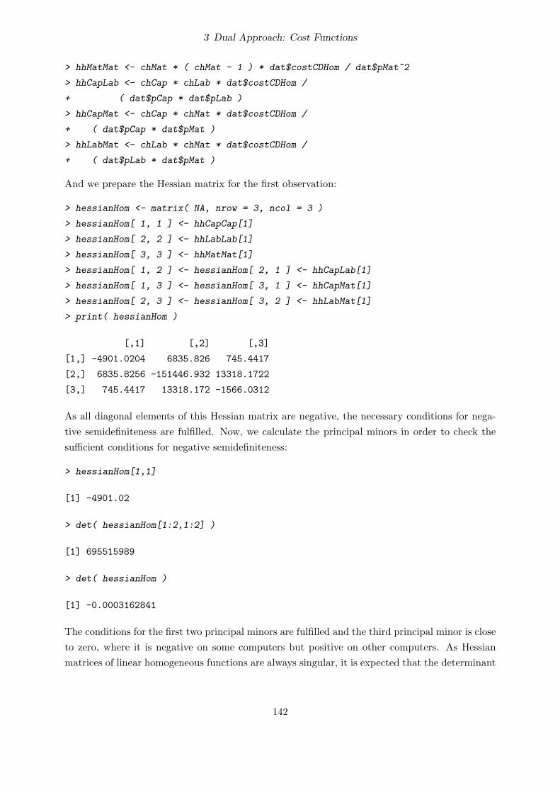
3 Dual Approach: Cost Functions
> hhMatMat <- chMat * ( chMat - 1 ) * dat$costCDHom / dat$pMat^2
> hhCapLab <- chCap * chLab * dat$costCDHom /
+ ( dat$pCap * dat$pLab )
> hhCapMat <- chCap * chMat * dat$costCDHom /
+ ( dat$pCap * dat$pMat )
> hhLabMat <- chLab * chMat * dat$costCDHom /
+ ( dat$pLab * dat$pMat )
And we prepare the Hessian matrix for the first observation:
> hessianHom <- matrix( NA, nrow = 3, ncol = 3 )
> hessianHom[ 1, 1 ] <- hhCapCap[1]
> hessianHom[ 2, 2 ] <- hhLabLab[1]
> hessianHom[ 3, 3 ] <- hhMatMat[1]
> hessianHom[ 1, 2 ] <- hessianHom[ 2, 1 ] <- hhCapLab[1]
> hessianHom[ 1, 3 ] <- hessianHom[ 3, 1 ] <- hhCapMat[1]
> hessianHom[ 2, 3 ] <- hessianHom[ 3, 2 ] <- hhLabMat[1]
> print( hessianHom )
[,1] [,2] [,3]
[1,] -4901.0204 6835.826 745.4417
[2,] 6835.8256 -151446.932 13318.1722
[3,] 745.4417 13318.172 -1566.0312
As all diagonal elements of this Hessian matrix are negative, the necessary conditions for nega-
tive semidefiniteness are fulfilled. Now, we calculate the principal minors in order to check the
sufficient conditions for negative semidefiniteness:
> hessianHom[1,1]
[1] -4901.02
> det( hessianHom[1:2,1:2] )
[1] 695515989
> det( hessianHom )
[1] -0.0003162841
The conditions for the first two principal minors are fulfilled and the third principal minor is close
to zero, where it is negative on some computers but positive on other computers. As Hessian
matrices of linear homogeneous functions are always singular, it is expected that the determinant
142

3 Dual Approach: Cost Functions
of the Hessian matrix (the Nth principal minor) is zero. However, the computed determinant of
our Hessian matrix is not exactly zero due to rounding errors, which are unavoidable on digital
computers. Given that the determinant of the Hessian matrix of our Cobb-Douglas cost function
with linear homogeneity imposed should always be zero, the Nth sufficient condition for negative
semidefiniteness (sign of the determinant of the Hessian matrix) should always be fulfilled. Con-
sequently, we can conclude that our Cobb-Douglas cost function with linear homogeneity imposed
is concave in input prices at the first observation. In order to avoid problems due to rounding
errors, we can just check the negative semidefiniteness of the first N − 1 rows and columns of the
Hessian matrix:
> semidefiniteness( hessianHom[1:2,1:2], positive = FALSE )
[1] TRUE
In the following, we will check whether concavity in input prices is fulfilled at each observation
in the sample:
> dat$concaveCDHom <- NA
> for( obs in 1:nrow( dat ) ) {
+ hessianPart <- matrix( NA, nrow = 2, ncol = 2 )
+ hessianPart[ 1, 1 ] <- hhCapCap[obs]
+ hessianPart[ 2, 2 ] <- hhLabLab[obs]
+ hessianPart[ 1, 2 ] <- hessianPart[ 2, 1 ] <- hhCapLab[obs]
+ dat$concaveCDHom[obs] <-
+ semidefiniteness( hessianPart, positive = FALSE )
+ }
> sum( !dat$concaveCDHom )
[1] 0
This result indicates that the concavity condition is violated not at a single observation. Con-
sequently, our Cobb-Douglas cost function with linear homogeneity imposed is concave in input
prices at all observations.
In fact, all Cobb-Douglas cost functions that are non-decreasing and linearly homogeneous in
all input prices are always concave (e.g. Coelli, 1995, p. 266).4
3.2.6 Optimal Cost Shares
Given Shepard’s Lemma, the optimal cost shares derived from a Cobb-Douglas cost function are
equal to the coefficients of the (logarithmic) input prices:
αi = ∂ ln c(w, y)∂ lnwi
= ∂c(w, y)∂wi
wi∂c(w, y) = xi(w, y) wi
c(w, y) = wi xi(w, y)c(w, y) = si(w, y), (3.26)
4 A proof and further details are available at http://www.econ.ucsb.edu/~tedb/Courses/GraduateTheoryUCSB/concavity.pdf.
143

3 Dual Approach: Cost Functions
where si = wi xi/c are the cost shares.
The following commands draw histograms of the observed cost shares and compare them to
the optimal cost shares, which are predicted by our Cobb-Douglas cost function with linear
homogeneity imposed:
> hist( dat$pCap * dat$qCap / dat$cost )
> lines( rep( chCap, 2), c( 0, 100 ), lwd = 3 )
> hist( dat$pLab * dat$qLab / dat$cost )
> lines( rep( chLab, 2), c( 0, 100 ), lwd = 3 )
> hist( dat$pMat * dat$qMat / dat$cost )
> lines( rep( chMat, 2), c( 0, 100 ), lwd = 3 )
cost share Cap
Fre
quen
cy
0.0 0.1 0.2 0.3 0.4
05
1015
2025
3035
cost share Lab
Fre
quen
cy
0.3 0.4 0.5 0.6 0.7 0.8
05
1015
2025
30
cost share Mat
Fre
quen
cy0.1 0.2 0.3 0.4 0.5 0.6
05
1015
2025
30
Figure 3.1: Observed and optimal costs shares
The resulting graphs are shown in figure 3.1. These results confirm results based on the production
function: most firms should increase the use of materials and decrease the use of capital goods.
3.2.7 Derived Input Demand Functions
Shepard’s Lemma says that the partial derivatives of the cost functions with respect to the input
prices are the conditional input demand functions. Therefore, the input demand functions based
on a Cobb-Douglas cost function are equal to the right-hand side of equation (3.20):
xi(w, y) = ∂c(w, y)∂wi
= αic(w, y)wi
(3.27)
Input demand functions should be homogeneous of degree zero in input prices:
xi(t w, y) = xi(w, y) (3.28)
144
3 Dual Approach: Cost Functions
This condition is fulfilled for the input demand functions derived from any linearly homogeneous
Cobb-Douglas cost function:
xi(t w, y) = αic(t w, y)t wi
= αit c(w, y)t wi
= αic(w, y)wi
= xi(w, y) (3.29)
Furthermore, input demand functions should be symmetric with respect to input prices:
∂xi(t w, y)∂wj
= ∂xj(t w, y)∂wi
(3.30)
This condition is fulfilled for the input demand functions derived from any Cobb-Douglas cost
function:
∂xi(w, y)∂wj
= αiwi
∂c(w, y)∂wj
= αiwi
αjc(w, y)wj
= αi αjwi wj
c(w, y) ∀ i 6= j (3.31)
∂xj(w, y)∂wi
= αjwj
∂c(w, y)∂wi
= αjwj
αic(w, y)wi
= αi αjwi wj
c(w, y) ∀ i 6= j (3.32)
Finally, input demand functions should fulfill the negativity condition:
∂xi(t w, y)∂wi
≤ 0 (3.33)
This condition is fulfilled for the input demand functions derived from any linearly homogeneous
Cobb-Douglas cost function that is monotonically increasing in all input prices (as this implies
0 ≤ αi ≤ 1):
∂xi(w, y)∂wi
= αiwi
∂c(w, y)∂wi
− αic(w, y)w2i
(3.34)
= αiwi
αic(w, y)wi
− αic(w, y)w2i
(3.35)
= αic(w, y)w2i
(αi − 1) ≤ 0 (3.36)
We can calculate the cost-minimizing input quantities that are predicted by a Cobb-Douglas
cost function by using equation (3.27). The following commands compare the observed input
quantities with the cost-minimizing input quantities that are predicted by our Cobb-Douglas
cost function with linear homogeneity imposed:
> compPlot( chCap * dat$costCDHom / dat$pCap, dat$qCap )
> compPlot( chLab * dat$costCDHom / dat$pLab, dat$qLab )
> compPlot( chMat * dat$costCDHom / dat$pMat, dat$qMat )
> compPlot( chCap * dat$costCDHom / dat$pCap, dat$qCap, log = "xy" )
> compPlot( chLab * dat$costCDHom / dat$pLab, dat$qLab, log = "xy" )
> compPlot( chMat * dat$costCDHom / dat$pMat, dat$qMat, log = "xy" )
145

3 Dual Approach: Cost Functions
●
●●●
●
●
●●
●
●
●
●
●
●●
●
●
●
●
●
●
●
●
●
●
●●
●
●●
●
●●
●
●
●●
● ●
●
●
●●
●
●●
●●
●
●●●
●●●
●●
●●
●
●
●
●
●●
●
●
●●
●
●
●
●
●
●●
●●
●●
●
●
●
●
●
●
●
●
●
●
●●
●
●
●
●
●
●
●
●
●
●
●●
●●●●
●
●●
●●
●●
●
●
●●
●
●
●●
●
●
●
●●
●
●
●
●
●
●
●●
●
●
●
●
0e+00 2e+05 4e+05
0e+
002e
+05
4e+
05
qCap optimal
qCap
obs
erve
d
●
●
●● ●
●
●●
●●
●
●●
●
●
●
●
●
●
●
●●●
●
●●
●
●
●●●● ●
● ●
●●● ● ●
●●
●●●●
●● ●●
●●
●
●
● ●●
●●
●
●●
●
●●
●●
●
●
●
●●●
●●
●
●●●● ●
●
●
●
●
●
●●●
●
●●
●
●
●
●
●●
●
●
●●
●●
●
●●●
●
●
●●●
●●●
●
●●
●●● ●●
●
●●
●
●
●●
●
●
●
●●
●
●
●
●
0 400000 800000 1200000
040
0000
8000
0012
0000
0
qLab optimal
qLab
obs
erve
d
●
●
●●
●
●
●
●
●
●
●●
●
●
●
●
●
●
●●
●●
● ●
●●
●
●
●●
●●●
● ● ●
●●
●●
●●●●●
●
●
●
●
●●●
●●
●●
●
●●
●
●
●
●
●
●
●
●●
●
●
● ● ●●
●
●
●
●
●●
●
●
●
●
●●
●
●
●
●
●●
●
●
●
●
●
●
●
●
●●
●
●●
●
●
●
●
●
●
●
●●
●● ●● ●
●
●●●
●
●
●●
●
●
●●
●
●
●
●
●
●
●
●
●
20000 60000 100000
2000
060
000
1000
00
qMat optimal
qMat
obs
erve
d
●
● ●
●
●
●
●●
●
●
●
●
●
●●
●
●
●
●
●
●
●
●
●
●
●
●
●
●
●
●
●
●
●
●
●
●
●●
●
●
●●
●
● ●
●●
●
●●●
●●
●
●
●●●
●
●
●
●
●●
●
●
●●
●
●
●
●
●
●
●
●●
●
●
●
●
●
●
●
●
●
●
●
●
●●
●
●
●
●
●
●
●
●
●
●
●●
●●
●
●
●
●●
●
●
●●
●
●
●●
●
●
●
●
●
●
●
●
●
●
●
●
●
●
●
●
●
●
●
●
●
5e+03 2e+04 1e+05 5e+05
5e+
032e
+04
1e+
055e
+05
qCap optimal
qCap
obs
erve
d
●
●
●
●●
●
●
●
●
●
●
●
●●
●
●
●
●
●
●
●●●
●
●
●
●
●
●
●●● ●
●●
●
●
●●
●
●●
●
●● ●
●● ●
●
●
●
●
●
● ●●
●
●
●
●
●
●
●●
●●
●
●
●
●●
●
●●
●
●
●●
●●
●
●
●
●
●
●●
●
●
●
●
●
●
●
●
●
●
●
●
●●
●●
●
●
●●
●
●
●● ●
●●
●
●
●
●
●
●●●
●
●
●
●
●
●
●●
●
●
●
●
●
●
●
●
●
5e+04 2e+05 5e+05
5e+
042e
+05
5e+
05
qLab optimal
qLab
obs
erve
d
●
●
●
●
●
●
●
●
●
●
●
●
●
●
●
●
●
●
●
●
●●
●●
●
●
●
●
●
●
●
●
●
● ● ●
●
●
●●
●
●●
●●
●
●
●
●
● ●
●
●
●
●
●
●
●●
●
●
●
●
●
●
●
●●
●
●
●● ●
●
●
●
●
●
●
●
●
●
●
●
●●
●
●
●
●
●
●
●●
●
●
●
●
●
●
●●
●
●
●
●
●
●
●
●
●
●
●
●
●
●●●
●
●
●●
●
●
●
●
●
●
●
●
●
●
●
●
●
●
●
●
●
●
5e+03 2e+04 5e+04
5e+
032e
+04
5e+
04
qMat optimal
qMat
obs
erve
d
Figure 3.2: Observed and optimal input quantities
146

3 Dual Approach: Cost Functions
The resulting graphs are shown in figure 3.2. These results confirm earlier results: most firms
should increase the use of materials and decrease the use of capital goods.
3.2.8 Derived Input Demand Elasticities
Based on the derived input demand functions (3.27), we can derive the conditional input demand
elasticities:
εij(w, y) = ∂xi(w, y)∂wj
wjxi(w, y) (3.37)
= αiwi
∂c(w, y)∂wj
wjxi(w, y) − δij αi
c(w, y)w2j
wjxi(w, y) (3.38)
= αiwi
αjc(w, y)wj
wjxi(w, y) − δij αi
c(w, y)wi xi(w, y) (3.39)
= αi αjc(w, y)
wi xi(w, y) − δijαi
si(w, y) (3.40)
= αi αjsi(w, y) − δij
αisi(w, y) (3.41)
= αj − δij (3.42)
εiy(w, y) = ∂xi(w, y)∂y
y
xi(w, y) (3.43)
= ∂c(w, y)∂y
αiwi
y
xi(w, y) (3.44)
= αyc(w, y)y
αiwi
y
xi(w, y) (3.45)
= αiαyc(w, y)y
y
wi xi(w, y) (3.46)
= αiαyc(w, y)
wi xi(w, y) (3.47)
= αyαi
si(w, y) (3.48)
= αy (3.49)
All derived input demand elasticities based on our estimated Cobb-Douglas cost function with
linear homogeneity imposed are presented in table 3.1. If the price of capital increases by one
percent, the cost-minimizing firm will decrease the use of capital by 0.93% and increase the
use of labor and materials by 0.07% each. If the price of labor increases by one percent, the
cost-minimizing firm will decrease the use of labor by 0.55% and increase the use of capital and
materials by 0.45% each. If the price of materials increases by one percent, the cost-minimizing
firm will decrease the use of materials by 0.52% and increase the use of capital and labor by
0.48% each. If the cost-minimizing firm increases the output quantity by one percent, (s)he will
147

3 Dual Approach: Cost Functions
increase all input quantities by 0.37%. The price elasticities derived from the Cobb-Douglas cost
function with linear homogeneity imposed are rather similar to the price elasticities derived from
the Cobb-Douglas production function but the elasticities with respect to the output quantity are
rather dissimilar (compare Tables 2.1 and 3.1). In theory, elasticities derived from a cost function,
which corresponds to a specific production function, should be identical to elasticities which are
directly derived from the production function. However, although our production function and
cost function are supposed to model the same production technology, their elasticities are not
the same. These differences arise from different econometric assumptions (e.g. exogeneity of
explanatory variables) and the disturbance terms, which differ between both models so that the
production technology is fitted differently.
Table 3.1: Conditional demand elasticities derived from Cobb-Douglas cost function (with linearhomogeneity imposed)
wcap wlab wmat y
xcap -0.93 0.45 0.48 0.37xlab 0.07 -0.55 0.48 0.37xmat 0.07 0.45 -0.52 0.37
Given Euler’s theorem and the cost function’s homogeneity in input prices, following condition
for the price elasticities can be obtained:
∑j
εij = 0 ∀ i (3.50)
The input demand elasticities derived from any linearly homogeneous Cobb-Douglas cost function
fulfill the homogeneity condition:
∑j
εij(w, y) =∑j
(αj − δij) =∑j
αj −∑j
δij = 1− 1 = 0 ∀ i (3.51)
As we computed the elasticities in table 3.1 based on the Cobb-Douglas function with linear
homogeneity imposed, these conditions are fulfilled for these elasticities.
It follows from the necessary conditions for the concavity of the cost function that all own-price
elasticities are non-positive:
εii ≤ 0 ∀ i (3.52)
The input demand elasticities derived from any linearly homogeneous Cobb-Douglas cost function
that is monotonically increasing in all input prices fulfill the negativity condition, because linear
homogeneity (∑i αi = 1) and monotonicity (αi ≥ 0 ∀ i) together imply that all αis (optimal cost
shares) are between zero and one (0 ≤ αi ≤ 1 ∀ i):
εii = αi − 1 ≤ 0 ∀ i (3.53)
148

3 Dual Approach: Cost Functions
As our Cobb-Douglas function with linear homogeneity imposed fulfills the homogeneity, mono-
tonicity, and concavity condition, the elasticities in table 3.1 fulfill the negativity conditions.
The symmetry condition for derived demand elasticities
siεij = sjεji ∀ i, j (3.54)
is fulfilled for any Cobb-Douglas cost function:
siεij(w, y) = αiαj = αjαi = sjεji ∀ i 6= j ∀ i, j (3.55)
Hence, the symmetry condition is also fulfilled for the elasticities in table 3.1, e.g. scap εcap,lab =αcap εcap,lab = 0.07 · 0.45 is equal to slab εlab,cap = αlab εlab,cap = 0.45 · 0.07.
3.2.9 Cost flexibility and elasticity of size
The coefficient of the (logarithmic) output quantity is equal to the “cost flexibility” (3.3). A value
of 0.37 (as in our estimated Cobb-Douglas cost function with linear homogeneity in input prices
imposed) means that a 1% increase in the output quantity results in a cost increase of 0.37%. The
“elasticity of size” is the inverse of the cost flexibility (3.4). A value of 2.67 (as derived from our
estimated Cobb-Douglas cost function with linear homogeneity in input prices imposed) means
that if costs are increased by 1%, the output quantity increases by 2.67%.
3.2.10 Marginal Costs, Average Costs, and Total Costs
Marginal costs can be calculated by
∂c(w, y)∂y
= αyc(w, y)y
(3.56)
These marginal costs should be linearly homogeneous in input prices:
∂c(t w, y)∂y
= t∂c(w, y)∂y
(3.57)
This condition is fulfilled for the marginal costs derived from a linearly homogeneous Cobb-
Douglas cost function:
∂c(t w, y)∂y
= αyc(t w, y)
y= αy
t c(w, y)y
= t αyc(w, y)y
= t∂c(w, y)∂y
(3.58)
We can compute the marginal costs by following command:
> chOut <- coef( costCDHom )[ "log(qOut)" ]
> dat$margCost <- chOut * dat$costCDHom / dat$qOut
We can visualize these marginal costs with a histogram.
149

3 Dual Approach: Cost Functions
> hist( dat$margCost, 20 )
margCost
Fre
quen
cy0.0 0.1 0.2 0.3 0.4 0.5
05
1525
Figure 3.3: Marginal costs
The resulting graph is shown in figure 3.3. It indicates that producing one additional output unit
increases the costs of most firms by around 0.08 monetary units.
Furthermore, we can check if the marginal costs are equal to the output prices, which is a
first-order condition for profit maximization:
> compPlot( dat$pOut, dat$margCost )
> compPlot( dat$pOut, dat$margCost, log = "xy" )
●● ●● ●
●●● ●● ●● ●●●
●
●●
●
●● ●●● ●●●●
●●●● ●●
●●
●●
●● ●●● ●
●
●●●●●● ●
●
●●● ●
●●
●
●
●● ●● ●● ● ●● ●● ●
●
●●●
●
●●
●● ●● ●● ●●
●●●● ●● ●●●●
● ●●● ●● ●●
●●
● ●●● ●●●
●
● ●●
● ●●●● ● ●●●●●● ●
● ●●●
● ●●●
0.0 0.5 1.0 1.5 2.0 2.5 3.0
0.0
0.5
1.0
1.5
2.0
2.5
3.0
pOut
mar
gCos
t
●●
●
●●
●●
● ●● ●●
●
●
●
●
●
●
●
●
●
●
●
●
●
●●
●
●
●●
●●●
●
●
●●
●●
●●
● ●
●
●●●
●
●●
●
●
●
●
● ●
●
●
●
●
●
●●
●
●
●●
●
●
●●
●
●
●●
●
●
●
●
●
●
●
●
●● ●
●
●
●
●●
●●
●
●
●
●
●
●●●
●
●
●
●
●
●
●
●●
● ●
●
●
●
●●
●
●
●●●
●
●
●●●
●
●●
●
●
●
●●
●
●
●
●
0.02 0.10 0.50 2.00
0.02
0.10
0.50
2.00
pOut
mar
gCos
t
Figure 3.4: Marginal costs and output prices
The resulting graphs are shown in figure 3.4. The marginal costs of all firms are considerably
smaller than their output prices. Hence, all firms would gain from increasing their output level.
This is not surprising for a technology with large economies of scale.
Now, we analyze, how the marginal costs depend on the output quantity:
> plot( dat$qOut, dat$margCost )
> plot( dat$qOut, dat$margCost, log = "xy" )
150

3 Dual Approach: Cost Functions
●●
●
●
●
●●●●
●●●
●
●
●
●
●
●
●
●●
●
●
●
●
●●
●
●
●●
●
●●
●
●
●
●
●●
●●● ●
●
●●●
●
●●
●
●
●
●
●●
●
●
●
●
●
●●
●
●●
●●
●
●●
●
●
●●
●
●
●
●
●
●
●
●
●●●
●
●●
●●
●●
●
●
●
●
●
●● ●
●
●●
●
●
●
●
●●
●●
●
●
●
●
●
●
●
●●●
●
●
●●●
●
●●
●
●
●
●●
●●
●
●
0.0e+00 1.0e+07 2.0e+07
0.1
0.2
0.3
0.4
0.5
qOut
mar
gCos
t●
●
●
●
●
●●
● ●
●● ●
●
●
●
●
●
●
●
●
●
●
●
●
●
●●
●
●
●●
●
●●
●
●
●
●
●
●
●●
● ●
●
●●●
●
●
●
●
●
●
●
●●
●
●
●
●
●
●
●●
●
●●
●
●
●
●
●
●
●●
●
●
●
●
●
●
●
●
●●●
●
●
●
●●
●
●
●
●
●
●
●
●● ●
●
●
●
●
●
●
●
●
●
●●
●
●
●
●
●
●
●
●●
●
●
●
●●●
●
●●
●
●
●
●●
●
●
●
●
1e+05 5e+05 5e+06
0.05
0.10
0.20
0.50
qOut
mar
gCos
t
Figure 3.5: Marginal costs depending on output quantity and firm size
The resulting graphs are shown in figure 3.5. Due to the large economies of size, the marginal
costs are decreasing with the output quantity.
The relation between output quantity and marginal costs in a Cobb-Douglas cost function can
be analyzed by taking the first derivative of the marginal costs (3.56) with respect to the output
quantity:
∂MC
∂y=∂(αy
c(w,y)y
)∂y
(3.59)
= αyy
∂c(w, y)∂y
− αyc(w, y)y2 (3.60)
= αyyαyc(w, y)y
− αyc(w, y)y2 (3.61)
= αyc
y2 (αy − 1) (3.62)
As αy, c, and y2 should always be positive, the marginal costs are (globally) increasing in the
output quantity, if there are decreasing returns to size (i.e. αy > 1) and the marginal costs are
(globally) decreasing in the output quantity, if there are increasing returns to size (i.e. αy < 1).
Now, we illustrate our estimated model by drawing the total cost curve for output quantities
between 0 and the maximum output level in the sample, where we use the sample means of the
input prices. Furthermore, we draw the average cost curve and the marginal cost curve for the
above-mentioned output quantities and input prices:
> y <- seq( 0, max( dat$qOut ), length.out = 200 )
> chInt <- coef(costCDHom)[ "(Intercept)" ]
> costs <- exp( chInt + chCap * log( mean( dat$pCap ) ) +
+ chLab * log( mean( dat$pLab ) ) + chMat * log( mean( dat$pMat ) ) +
+ chOut * log( y ) )
151

3 Dual Approach: Cost Functions
> plot( y, costs, type = "l" )
> # average costs
> plot( y, costs/y, type = "l" )
> # marginal costs
> lines( y, chOut * costs / y, lty = 2 )
> legend( "right", lty = c( 1, 2 ),
+ legend = c( "average costs", "marginal costs" ) )
0.0e+00 1.0e+07 2.0e+07
040
0000
8000
00
y
tota
l cos
ts
0.0e+00 1.0e+07 2.0e+07
0.0
0.4
0.8
1.2
y
aver
age
cost
s, m
argi
nal c
osts
average costsmarginal costs
Figure 3.6: Total, marginal, and average costs
The resulting graphs are shown in figure 3.6. As the marginal costs are equal to the average costs
multiplied by a fixed factor, αy (see equation 3.56), the average cost curve and the marginal cost
curve of a Cobb-Douglas cost function cannot intersect.
3.3 Cobb-Douglas Short-Run Cost Function
3.3.1 Specification
Given the general specification of a short-run cost function (3.5), a Cobb-Douglas short-run cost
function is
cv = A
∏i∈N1
wαii
∏j∈N2
xαjj
yαy , (3.63)
where cv denotes the variable costs as defined in (1.3), N1 is a vector of the indices of the variable
inputs, and N2 is a vector of the indices of the quasi-fixed inputs. The Cobb-Douglas short-run
152

3 Dual Approach: Cost Functions
cost function can be linearized to
ln cv = α0 +∑i∈N1
αi lnwi +∑j∈N2
αj ln xj + αy ln y (3.64)
with α0 = lnA.
3.3.2 Estimation
The following commands estimate a Cobb-Douglas short-run cost function with capital as a
quasi-fixed input and summarize the results:
> costCDSR <- lm( log( vCost ) ~ log( pLab ) + log( pMat ) + log( qCap ) + log( qOut ),
+ data = dat )
> summary( costCDSR )
Call:
lm(formula = log(vCost) ~ log(pLab) + log(pMat) + log(qCap) +
log(qOut), data = dat)
Residuals:
Min 1Q Median 3Q Max
-0.73935 -0.20934 -0.00571 0.20729 0.71633
Coefficients:
Estimate Std. Error t value Pr(>|t|)
(Intercept) 5.66013 0.42523 13.311 < 2e-16 ***
log(pLab) 0.45683 0.13819 3.306 0.00121 **
log(pMat) 0.44144 0.07715 5.722 6.50e-08 ***
log(qCap) 0.19174 0.04034 4.754 5.05e-06 ***
log(qOut) 0.29127 0.03318 8.778 6.49e-15 ***
---
Signif. codes: 0 ‘***’ 0.001 ‘**’ 0.01 ‘*’ 0.05 ‘.’ 0.1 ‘ ’ 1
Residual standard error: 0.3183 on 135 degrees of freedom
Multiple R-squared: 0.7265, Adjusted R-squared: 0.7183
F-statistic: 89.63 on 4 and 135 DF, p-value: < 2.2e-16
3.3.3 Properties
This short-run cost function is (significantly) increasing in the prices of the variable inputs (labor
and materials) as the coefficient of the labor price (0.457) and the coefficient of the materials
153

3 Dual Approach: Cost Functions
price (0.441) are both positive. However, this short-run cost function is not linearly homogeneous
in input prices, as the coefficient of the labor price and the coefficient of the materials price do not
sum up to one (0.457 + 0.441 = 0.898). The short-run cost function is increasing in the output
quantity with a short-run cost flexibility of 0.291, which corresponds to a short-run elasticity of
size of 3.433. However, this short-run cost function is increasing in the quantity of the fixed input
(capital), as the corresponding coefficient is (significantly) positive (0.192) which contradicts
microeconomic theory. This would mean that the apple producers could reduce variable costs
(costs from labor and materials) by reducing the capital input (e.g. by destroying their apple trees
and machinery), while still producing the same amount of apples. Producing the same output
level with less of all inputs is not plausible.
3.3.4 Estimation with linear homogeneity in input prices imposed
We can impose linear homogeneity in the prices of the variable inputs as we did with the (long-
run) cost function (see equations 3.15 to 3.19):
ln c
wk= α0 +
∑i∈N1\k
αi ln wiwk
+∑j∈N2
αj ln xj + αy ln y (3.65)
with k ∈ N1. We can estimate a Cobb-Douglas short-run cost function with capital as a quasi-
fixed input and linear homogeneity in input prices imposed by the command:
> costCDSRHom <- lm( log( vCost / pMat ) ~ log( pLab / pMat ) +
+ log( qCap ) + log( qOut ), data = dat )
> summary( costCDSRHom )
Call:
lm(formula = log(vCost/pMat) ~ log(pLab/pMat) + log(qCap) + log(qOut),
data = dat)
Residuals:
Min 1Q Median 3Q Max
-0.78305 -0.20539 -0.00265 0.19533 0.71792
Coefficients:
Estimate Std. Error t value Pr(>|t|)
(Intercept) 5.67882 0.42335 13.414 < 2e-16 ***
log(pLab/pMat) 0.53487 0.06781 7.888 9.00e-13 ***
log(qCap) 0.18774 0.03978 4.720 5.79e-06 ***
log(qOut) 0.29010 0.03306 8.775 6.33e-15 ***
---
Signif. codes: 0 ‘***’ 0.001 ‘**’ 0.01 ‘*’ 0.05 ‘.’ 0.1 ‘ ’ 1
154

3 Dual Approach: Cost Functions
Residual standard error: 0.3176 on 136 degrees of freedom
Multiple R-squared: 0.5963, Adjusted R-squared: 0.5874
F-statistic: 66.97 on 3 and 136 DF, p-value: < 2.2e-16
We can obtain the coefficient of the materials price from the homogeneity condition (3.15): 1−0.535 = 0.465. We can test the homogeneity restriction by a likelihood ratio test:
> lrtest( costCDSRHom, costCDSR )
Likelihood ratio test
Model 1: log(vCost/pMat) ~ log(pLab/pMat) + log(qCap) + log(qOut)
Model 2: log(vCost) ~ log(pLab) + log(pMat) + log(qCap) + log(qOut)
#Df LogLik Df Chisq Pr(>Chisq)
1 5 -36.055
2 6 -35.838 1 0.4356 0.5093
Given the large P -value, we can conclude that the data do not contradict the linear homogeneity
in the prices of the variable inputs.
While the linear homogeneity in the prices of all variable inputs is accepted and the short-run
cost function is still increasing in the output quantity and the prices of all variable inputs, the
estimated short-run cost function is still increasing in the capital quantity, which contradicts
microeconomic theory. Therefore, a further microeconomic analysis with this function is not
reasonable.
3.4 Translog cost function
3.4.1 Specification
The general specification of a Translog cost function is
ln c(w, y) = α0 +N∑i=1
αi lnwi + αy ln y (3.66)
+ 12
N∑i=1
N∑j=1
αij lnwi lnwj + 12αyy (ln y)2
+N∑i=1
αiy lnwi ln y
with αij = αji ∀ i, j.
155

3 Dual Approach: Cost Functions
3.4.2 Estimation
The Translog cost function can be estimated by following command:
> costTL <- lm( log( cost ) ~ log( pCap ) + log( pLab ) + log( pMat ) +
+ log( qOut ) + I( 0.5 * log( pCap )^2 ) + I( 0.5 * log( pLab )^2 ) +
+ I( 0.5 * log( pMat )^2 ) + I( log( pCap ) * log( pLab ) ) +
+ I( log( pCap ) * log( pMat ) ) + I( log( pLab ) * log( pMat ) ) +
+ I( 0.5 * log( qOut )^2 ) + I( log( pCap ) * log( qOut ) ) +
+ I( log( pLab ) * log( qOut ) ) + I( log( pMat ) * log( qOut ) ),
+ data = dat )
> summary( costTL )
Call:
lm(formula = log(cost) ~ log(pCap) + log(pLab) + log(pMat) +
log(qOut) + I(0.5 * log(pCap)^2) + I(0.5 * log(pLab)^2) +
I(0.5 * log(pMat)^2) + I(log(pCap) * log(pLab)) + I(log(pCap) *
log(pMat)) + I(log(pLab) * log(pMat)) + I(0.5 * log(qOut)^2) +
I(log(pCap) * log(qOut)) + I(log(pLab) * log(qOut)) + I(log(pMat) *
log(qOut)), data = dat)
Residuals:
Min 1Q Median 3Q Max
-0.73251 -0.18718 0.02001 0.15447 0.82858
Coefficients:
Estimate Std. Error t value Pr(>|t|)
(Intercept) 25.383429 3.511353 7.229 4.26e-11 ***
log(pCap) 0.198813 0.537885 0.370 0.712291
log(pLab) -0.024792 2.232126 -0.011 0.991156
log(pMat) -1.244914 1.201129 -1.036 0.301992
log(qOut) -2.040079 0.510905 -3.993 0.000111 ***
I(0.5 * log(pCap)^2) -0.095173 0.105158 -0.905 0.367182
I(0.5 * log(pLab)^2) -0.503168 0.943390 -0.533 0.594730
I(0.5 * log(pMat)^2) 0.529021 0.337680 1.567 0.119728
I(log(pCap) * log(pLab)) -0.746199 0.244445 -3.053 0.002772 **
I(log(pCap) * log(pMat)) 0.182268 0.130463 1.397 0.164865
I(log(pLab) * log(pMat)) 0.139429 0.433408 0.322 0.748215
I(0.5 * log(qOut)^2) 0.164075 0.041078 3.994 0.000110 ***
I(log(pCap) * log(qOut)) -0.028090 0.042844 -0.656 0.513259
I(log(pLab) * log(qOut)) 0.007533 0.171134 0.044 0.964959
156

3 Dual Approach: Cost Functions
I(log(pMat) * log(qOut)) 0.048794 0.092266 0.529 0.597849
---
Signif. codes: 0 ‘***’ 0.001 ‘**’ 0.01 ‘*’ 0.05 ‘.’ 0.1 ‘ ’ 1
Residual standard error: 0.3043 on 125 degrees of freedom
Multiple R-squared: 0.7682, Adjusted R-squared: 0.7423
F-statistic: 29.59 on 14 and 125 DF, p-value: < 2.2e-16
As the Cobb-Douglas cost function is nested in the Translog cost function, we can use a
statistical test to check whether the Cobb-Douglas cost function fits the data as good as the
Translog cost function:
> lrtest( costCD, costTL )
Likelihood ratio test
Model 1: log(cost) ~ log(pCap) + log(pLab) + log(pMat) + log(qOut)
Model 2: log(cost) ~ log(pCap) + log(pLab) + log(pMat) + log(qOut) + I(0.5 *
log(pCap)^2) + I(0.5 * log(pLab)^2) + I(0.5 * log(pMat)^2) +
I(log(pCap) * log(pLab)) + I(log(pCap) * log(pMat)) + I(log(pLab) *
log(pMat)) + I(0.5 * log(qOut)^2) + I(log(pCap) * log(qOut)) +
I(log(pLab) * log(qOut)) + I(log(pMat) * log(qOut))
#Df LogLik Df Chisq Pr(>Chisq)
1 6 -44.867
2 16 -24.149 10 41.435 9.448e-06 ***
---
Signif. codes: 0 ‘***’ 0.001 ‘**’ 0.01 ‘*’ 0.05 ‘.’ 0.1 ‘ ’ 1
Given the very small P -value, we can conclude that the Cobb-Douglas cost function is not suitable
for analyzing the production technology in our data set.
3.4.3 Linear homogeneity in input prices
Linear homogeneity of a Translog cost function requires
ln(t c(w, y)) = ln c(t w, y) (3.67)
ln t+ ln c(w, y) = α0 +N∑i=1
αi ln(t wi) + αy ln y (3.68)
+ 12
N∑i=1
N∑j=1
αij ln(t wi) ln(t wj) + 12αyy (ln y)2
+N∑i=1
αiy ln(t wi) ln y
157

3 Dual Approach: Cost Functions
= α0 +N∑i=1
αi ln(t) +N∑i=1
αi ln(wi) + αy ln y (3.69)
+ 12
N∑i=1
N∑j=1
αij ln(t) ln(t) + 12
N∑i=1
N∑j=1
αij ln(t) ln(wj)
+ 12
N∑i=1
N∑j=1
αij ln(wi) ln(t) + 12
N∑i=1
N∑j=1
αij ln(wi) ln(wj)
+ 12αyy (ln y)2 +
N∑i=1
αiy ln(t) ln y +N∑i=1
αiy ln(wi) ln y
= α0 + ln(t)N∑i=1
αi +N∑i=1
αi ln(wi) + αy ln y (3.70)
+ 12 ln(t) ln(t)
N∑i=1
N∑j=1
αij + 12 ln(t)
N∑j=1
ln(wj)N∑i=1
αij
+ 12 ln(t)
N∑i=1
ln(wi)N∑j=1
αij + 12
N∑i=1
N∑j=1
αij ln(wi) ln(wj)
+ 12αyy (ln y)2 + ln(t) ln y
N∑i=1
αiy +N∑i=1
αiy ln(wi) ln y
= ln c(w, y) + ln(t)N∑i=1
αi (3.71)
+ 12 ln(t) ln(t)
N∑i=1
N∑j=1
αij + 12 ln(t)
N∑j=1
ln(wj)N∑i=1
αij
+ 12 ln(t)
N∑i=1
ln(wi)N∑j=1
αij + ln(t) ln yN∑i=1
αiy
ln t = ln(t)N∑i=1
αi + 12 ln(t) ln(t)
N∑i=1
N∑j=1
αij + 12 ln(t)
N∑j=1
ln(wj)N∑i=1
αij (3.72)
+ 12 ln(t)
N∑i=1
ln(wi)N∑j=1
αij + ln(t) ln yN∑i=1
αiy
1 =N∑i=1
αi + 12 ln(t)
N∑i=1
N∑j=1
αij + 12
N∑j=1
ln(wj)N∑i=1
αij (3.73)
+ 12
N∑i=1
ln(wi)N∑j=1
αij + ln yN∑i=1
αiy
Hence, the homogeneity condition is only globally fulfilled (i.e. no matter which values t, w, and
y have) if the following parameter restrictions hold:
N∑i=1
αi = 1 (3.74)
158

3 Dual Approach: Cost Functions
N∑i=1
αij = 0 ∀ j αij=αji←−−−−→N∑j=1
αij = 0 ∀ i (3.75)
N∑i=1
αiy = 0 (3.76)
We can see from the estimates above that these conditions are not fulfilled in our Translog cost
function. For instance, according to condition (3.74), the first-order coefficients of the input
prices should sum up to one but our estimates sum up to 0.199 + (−0.025) + (−1.245) = −1.071.
Hence, the homogeneity condition is not fulfilled in our estimated Translog cost function.
3.4.4 Estimation with linear homogeneity in input prices imposed
In order to impose linear homogeneity in input prices, we can rearrange these restrictions to get
αN = 1−N−1∑i=1
αi (3.77)
αNj = −N−1∑i=1
αij ∀ j (3.78)
αiN = −N−1∑j=1
αij ∀ i (3.79)
αNy = −N−1∑i=1
αiy (3.80)
Replacing αN , αNy and all αiN and αjN in equation (3.66) by the right-hand sides of equa-
tions (3.77) to (3.80) and re-arranging, we get
ln c(w, y)wN
= α0 +N−1∑i=1
αi ln wiwN
+ αy ln y (3.81)
+ 12
N−1∑j=1
N−1∑i=1
αij ln wiwN
ln wjwN
+ 12αyy (ln y)2
+N−1∑i=1
αiy ln wiwN
ln y.
This Translog cost function with linear homogeneity imposed can be estimated by following
command:
> costTLHom <- lm( log( cost / pMat ) ~ log( pCap / pMat ) +
+ log( pLab / pMat ) + log( qOut ) +
+ I( 0.5 * log( pCap / pMat )^2 ) + I( 0.5 * log( pLab / pMat )^2 ) +
+ I( log( pCap / pMat ) * log( pLab / pMat ) ) +
+ I( 0.5 * log( qOut )^2 ) + I( log( pCap / pMat ) * log( qOut ) ) +
159

3 Dual Approach: Cost Functions
+ I( log( pLab / pMat ) * log( qOut ) ),
+ data = dat )
> summary( costTLHom )
Call:
lm(formula = log(cost/pMat) ~ log(pCap/pMat) + log(pLab/pMat) +
log(qOut) + I(0.5 * log(pCap/pMat)^2) + I(0.5 * log(pLab/pMat)^2) +
I(log(pCap/pMat) * log(pLab/pMat)) + I(0.5 * log(qOut)^2) +
I(log(pCap/pMat) * log(qOut)) + I(log(pLab/pMat) * log(qOut)),
data = dat)
Residuals:
Min 1Q Median 3Q Max
-0.6860 -0.2086 0.0192 0.1978 0.8281
Coefficients:
Estimate Std. Error t value Pr(>|t|)
(Intercept) 23.714976 3.445289 6.883 2.24e-10 ***
log(pCap/pMat) 0.306159 0.525789 0.582 0.561383
log(pLab/pMat) 1.093860 1.169160 0.936 0.351216
log(qOut) -1.933605 0.501090 -3.859 0.000179 ***
I(0.5 * log(pCap/pMat)^2) 0.025951 0.089977 0.288 0.773486
I(0.5 * log(pLab/pMat)^2) 0.716467 0.338049 2.119 0.035957 *
I(log(pCap/pMat) * log(pLab/pMat)) -0.292889 0.142710 -2.052 0.042144 *
I(0.5 * log(qOut)^2) 0.158662 0.039866 3.980 0.000114 ***
I(log(pCap/pMat) * log(qOut)) -0.048274 0.040025 -1.206 0.229964
I(log(pLab/pMat) * log(qOut)) 0.008363 0.096490 0.087 0.931067
---
Signif. codes: 0 ‘***’ 0.001 ‘**’ 0.01 ‘*’ 0.05 ‘.’ 0.1 ‘ ’ 1
Residual standard error: 0.3089 on 130 degrees of freedom
Multiple R-squared: 0.6377, Adjusted R-squared: 0.6126
F-statistic: 25.43 on 9 and 130 DF, p-value: < 2.2e-16
We can use a likelihood ratio test to compare this function with the unconstrained Translog cost
function (3.66):
> lrtest( costTL, costTLHom )
Likelihood ratio test
160

3 Dual Approach: Cost Functions
Model 1: log(cost) ~ log(pCap) + log(pLab) + log(pMat) + log(qOut) + I(0.5 *
log(pCap)^2) + I(0.5 * log(pLab)^2) + I(0.5 * log(pMat)^2) +
I(log(pCap) * log(pLab)) + I(log(pCap) * log(pMat)) + I(log(pLab) *
log(pMat)) + I(0.5 * log(qOut)^2) + I(log(pCap) * log(qOut)) +
I(log(pLab) * log(qOut)) + I(log(pMat) * log(qOut))
Model 2: log(cost/pMat) ~ log(pCap/pMat) + log(pLab/pMat) + log(qOut) +
I(0.5 * log(pCap/pMat)^2) + I(0.5 * log(pLab/pMat)^2) + I(log(pCap/pMat) *
log(pLab/pMat)) + I(0.5 * log(qOut)^2) + I(log(pCap/pMat) *
log(qOut)) + I(log(pLab/pMat) * log(qOut))
#Df LogLik Df Chisq Pr(>Chisq)
1 16 -24.149
2 11 -29.014 -5 9.7309 0.08323 .
---
Signif. codes: 0 ‘***’ 0.001 ‘**’ 0.01 ‘*’ 0.05 ‘.’ 0.1 ‘ ’ 1
The null hypothesis, linear homogeneity in input prices, is rejected at the 10% significance level
but not at the 5% level. Given the importance of microeconomic consistency and that 5% is the
standard significance level, we continue our analysis with the Translog cost function with linear
homogeneity in input prices imposed.
Furthermore, we can use a likelihood ratio test to compare this function with the Cobb-Douglas
cost function with homogeneity imposed (3.19):
> lrtest( costCDHom, costTLHom )
Likelihood ratio test
Model 1: log(cost/pMat) ~ log(pCap/pMat) + log(pLab/pMat) + log(qOut)
Model 2: log(cost/pMat) ~ log(pCap/pMat) + log(pLab/pMat) + log(qOut) +
I(0.5 * log(pCap/pMat)^2) + I(0.5 * log(pLab/pMat)^2) + I(log(pCap/pMat) *
log(pLab/pMat)) + I(0.5 * log(qOut)^2) + I(log(pCap/pMat) *
log(qOut)) + I(log(pLab/pMat) * log(qOut))
#Df LogLik Df Chisq Pr(>Chisq)
1 5 -44.878
2 11 -29.014 6 31.727 1.84e-05 ***
---
Signif. codes: 0 ‘***’ 0.001 ‘**’ 0.01 ‘*’ 0.05 ‘.’ 0.1 ‘ ’ 1
Again, the Cobb-Douglas functional form is clearly rejected by the data in favor of the Translog
functional form.
Some parameters of the Translog cost function with linear homogeneity imposed (3.81) have
not been directly estimated (αN , αNy, all αiN , all αjN ) but they can be retrieved from the
161

3 Dual Approach: Cost Functions
(directly) estimated parameters and equations (3.77) to (3.80). Please note that the specification
in equation (3.81) is used for the econometric estimation only; after retrieving the non-estimated
parameters, we can do our analysis based on equation (3.66). To facilitate the further analysis,
we create short-cuts of all estimated parameters and obtain the parameters that have not been
directly estimated:
> ch0 <- coef( costTLHom )[ "(Intercept)" ]
> ch1 <- coef( costTLHom )[ "log(pCap/pMat)" ]
> ch2 <- coef( costTLHom )[ "log(pLab/pMat)" ]
> ch3 <- 1 - ch1 - ch2
> chy <- coef( costTLHom )[ "log(qOut)" ]
> ch11 <- coef( costTLHom )[ "I(0.5 * log(pCap/pMat)^2)" ]
> ch22 <- coef( costTLHom )[ "I(0.5 * log(pLab/pMat)^2)" ]
> chyy <- coef( costTLHom )[ "I(0.5 * log(qOut)^2)" ]
> ch12 <- ch21 <- coef( costTLHom )[ "I(log(pCap/pMat) * log(pLab/pMat))" ]
> ch13 <- ch31 <- 0 - ch11 - ch12
> ch23 <- ch32 <- 0 - ch12 - ch22
> ch33 <- 0 - ch13 - ch23
> ch1y <- coef( costTLHom )[ "I(log(pCap/pMat) * log(qOut))" ]
> ch2y <- coef( costTLHom )[ "I(log(pLab/pMat) * log(qOut))" ]
> ch3y <- 0 - ch1y - ch2y
Hence, our estimated Translog cost function has following parameters:
> # alpha_0, alpha_i, alpha_y
> unname( c( ch0, ch1, ch2, ch3, chy ) )
[1] 23.7149761 0.3061589 1.0938598 -0.4000187 -1.9336052
> # alpha_ij
> matrix( c( ch11, ch12, ch13, ch21, ch22, ch23, ch31, ch32, ch33 ), ncol=3 )
[,1] [,2] [,3]
[1,] 0.02595083 -0.2928892 0.2669384
[2,] -0.29288920 0.7164670 -0.4235778
[3,] 0.26693837 -0.4235778 0.1566394
> # alpha_iy, alpha_yy
> unname( c( ch1y, ch2y, ch3y, chyy ) )
[1] -0.048274484 0.008362717 0.039911768 0.158661757
162

3 Dual Approach: Cost Functions
3.4.5 Cost Flexibility and Elasticity of Size
Based on the estimated parameters, we can calculate the cost flexibilities and the elasticities of
size. The cost flexibilities derived from a Translog cost function (3.66) are
∂ ln c(w, y)∂ ln y = αy +
N∑i=1
αiy lnwi + αyy ln y (3.82)
and the elasticities of size are—as always—their inverses:
∂ ln y∂ ln c =
(∂ ln c(w, y)∂ ln y
)−1(3.83)
We can calculate the cost flexibilities and the elasticities of size with following commands:
> dat$costFlex <- with( dat, chy + ch1y * log( pCap ) +
+ ch2y * log( pLab ) + ch3y * log( pMat ) + chyy * log( qOut ) )
> dat$elaSize <- 1 / dat$costFlex
Now, we can visualize these values using histograms:
> hist( dat$costFlex )
> hist( dat$elaSize )
> hist( dat$elaSize[ dat$elaSize > 0 & dat$elaSize < 10 ] )
cost flexibility
Fre
quen
cy
0.0 0.2 0.4 0.6 0.8
05
1015
2025
3035
elasticity of size
Fre
quen
cy
−20 0 20 40 60 80 100
020
4060
8012
0
elasticity of size
Fre
quen
cy
2 4 6 8 10
010
2030
4050
60
Figure 3.7: Translog cost function: cost flexibility and elasticity of size
The resulting graphs are presented in figure 3.7. Only 1 out of 140 cost flexibilities is negative.
Hence, the estimated Translog cost function is to a very large extent increasing in the output
quantity. All cost flexibilities are lower than one, which indicates that all apple producers operate
under increasing returns to size. Most cost flexibilities are around 0.5, which corresponds to an
elasticity of size of 2. Hence, if the apple producers increase their output quantity by one percent,
the total costs of most producers increases by around 0.5 percent. Or—the other way round—if
163

3 Dual Approach: Cost Functions
the apple producers increase their input use so that their costs increase by one percent, the output
quantity of most producers would increase by around two percent.
With the following commands, we visualize the relationship between output quantity and
elasticity of size
> plot( dat$qOut, dat$elaSize )
> abline( 1, 0 )
> plot( dat$qOut, dat$elaSize, ylim = c( 0, 10 ) )
> abline( 1, 0 )
> plot( dat$qOut, dat$elaSize, ylim = c( 0, 10 ), log = "x" )
> abline( 1, 0 )
●● ●●● ●●●●●●●●●
●●
●●
●
● ●●●●●●● ●
●
●●●
●●●●
●
●
●● ●●● ●●
●●●●●●●
●
●●●●●
●
●
●● ● ●● ●●● ● ●●● ●
●
● ●●●●●
● ●● ●●●●● ● ●●● ●●● ●● ●● ●● ●●● ●● ●● ●●●●●●●
●
●● ●●●● ●●●●●● ●●● ●● ●●● ●●● ●
0.0e+00 1.0e+07 2.0e+07
−20
020
4060
8010
0
qOut
dat$
elaS
ize
●
●
●
●
●
●●
●●●●
●●●
●
●
●
●●●
●
●●
●
●●
●
●
●●
●
●●●
●
●
●●●
●
●
●
●●●
●
●●●
●
●
●
●
●
●
●
●
● ●
●
●●● ●
●
●●
●
●
●●
●
●
●
●
●●●
●●●●
●
●
●●●●
●
●
●
●
●●●●●
●
●
●
●
●
●●
●●●●
●●
●
●●
●●
●●●
●●
●
●
●●●
●
●
●
●
●●
●
●
0.0e+00 1.0e+07 2.0e+07
02
46
810
qOut
dat$
elaS
ize
●
●
●
●
●
●●
● ●●●
●●
●
●
●
●
● ●●
●
●●
●
●●
●
●
●●
●
●●●
●
●
●●●
●
●
●
●●●
●
●●●
●
●
●
●
●
●
●
●
● ●
●
●●● ●
●
●●
●
●
● ●
●
●
●
●
●●●
●●●●
●
●
●●●●
●
●
●
●
●●●● ●
●
●
●
●
●
●●
●●●●
●●
●
●●
●●
●●●
●●
●
●
●●●
●
●
●
●
●●
●
●
1e+05 5e+05 5e+06
02
46
810
qOutda
t$el
aSiz
e
Figure 3.8: Translog cost function: output quantity and elasticity of size
The resulting graphs are shown in figure 3.8. With increasing output quantity, the elasticity of
size approaches one (from above). Hence, small apple producers could gain a lot from increasing
their size, while large apple producers would gain much less from increasing their size. However,
even the largest producers still gain from increasing their size so that the optimal firm size is
larger than the largest firm in the sample.
3.4.6 Marginal Costs and Average Costs
Marginal costs derived from a Translog cost function are
∂c(w, y)∂y
= ∂ ln c(w, y)∂ ln y
c(w, y)y
=(αy +
N∑i=1
αiy lnwi + αyy ln y)c(w, y)y
. (3.84)
Hence, they are—as always—equal to the cost flexibility multiplied by total costs and divided
by the output quantity. We can compute the total costs that are predicted by our estimated
Translog cost function by following command:
> dat$costTLHom <- exp( fitted( costTLHom ) ) * dat$pMat
164

3 Dual Approach: Cost Functions
Now, we can compute the marginal costs by:
> dat$margCostTL <- with( dat, costFlex * costTLHom / qOut )
We can visualize these marginal costs with a histogram.
> hist( dat$margCostTL, 15 )
margCostTL
Fre
quen
cy
−0.15 −0.05 0.05 0.15
020
40
Figure 3.9: Translog cost function: Marginal costs
The resulting graph is shown in figure 3.9. It indicates that producing one additional output unit
increases the costs of most firms by around 0.09 monetary units.
Furthermore, we can check if the marginal costs are equal to the output prices, which is a
first-order condition for profit maximization:
> compPlot( dat$pOut, dat$margCostTL )
> compPlot( dat$pOut[ dat$margCostTL > 0 ],
+ dat$margCostTL[ dat$margCostTL > 0 ], log = "xy" )
●● ●● ● ●●● ●● ●● ●●● ●●● ● ●● ●●● ●●●● ●●●●
●●●● ●
●
●● ●●● ●●●●●●●● ●
●●●● ●●●
●●● ● ●● ●● ● ●● ●● ●●●●●●●●● ●
●● ●● ●● ●●●● ●● ●●●●● ●●● ●● ●●●●● ●●● ●●●●● ●●● ●●●●
● ●●● ●●● ●● ●●● ● ● ●●
0.0 0.5 1.0 1.5 2.0 2.5 3.0
0.0
1.0
2.0
3.0
pOut
mar
gCos
tTL
●●
●
●● ●●
● ●● ●●
●●●
●●
●
●●●●
●
● ●●●
●●●
●●
●
●
●
●
●
●● ●●●
●●
●●●
●
●●
●
●
●●● ●
●
●
●●
●●
●
●
●●● ●●
●
● ●●
●
●
●
●●●●
●
●
●●●
●●
●●●●
●● ●
●●
●
●
●●
●
●
●●●
●
●
●
●●
● ●
●
●
●
● ●
●
●
●●●
●
●
●●●●
●●
●
●●
●● ●●
●
●
0.02 0.10 0.50 2.00
0.02
0.10
0.50
2.00
pOut
mar
gCos
tTL
Figure 3.10: Translog cost function: marginal costs and output prices
The resulting graphs are shown in figure 3.10. The marginal costs of all firms are considerably
smaller than their output prices. Hence, all firms would gain from increasing their output level.
This is not surprising for a technology with large economies of scale.
165

3 Dual Approach: Cost Functions
Now, we analyze, how the marginal costs depend on the output quantity:
> plot( dat$qOut, dat$margCostTL )
> plot( dat$qOut, dat$margCostTL, log = "x" )
●
●
●
●
●●
●●●●
●
●●
●●
●
●
●
●
● ●●
●
●●●●
●
● ●●
●
●
●
●
●
●
●
●● ●●●
●
●
●●●
●
●●
●
●
●
●●●
●
●
●
●
●●
●
●
●●●●
●●
●●
●
●
●
●
●
●●●
●
●
●
●●●
●
●●
●●
●
●●
●●
●
●
●●
●
●
●
●●
●
●
●
●●
●●
●
●
●
●●
●
●
●● ●
●
●
●●●
●●●
●
●
●
●● ●
●
●
●
0.0e+00 1.0e+07 2.0e+07
−0.
15−
0.05
0.05
0.15
qOut
mar
gCos
t
●
●
●
●
●●
●● ●●
●
●●
●●
●
●
●
●
● ●●
●
●●
●●
●
● ●●
●
●
●
●
●
●
●
● ● ●●●
●
●
●●●
●
●●
●
●
●
● ●●
●
●
●
●
●●
●
●
●●●●
●●
●●
●
●
●
●
●
●● ●
●
●
●
●●●
●
●●
●●
●
●●
●●
●
●
●●
●
●
●
●●
●
●
●
●●
●●
●
●
●
●●
●
●
●● ●
●
●
●●
●
●●●
●
●
●
●● ●
●
●
●
1e+05 5e+05 5e+06
−0.
15−
0.05
0.05
0.15
qOutm
argC
ost
Figure 3.11: Translog cost function: Marginal costs depending on output quantity
The resulting graphs are shown in figure 3.11. There is no clear relationship between marginal
costs and the output quantity.
Now, we illustrate our estimated model by drawing the average cost curve and the marginal
cost curve for output quantities between 0 and five times the maximum output level in the sample,
where we use the sample means of the input prices.
> y <- seq( 0, 5 * max( dat$qOut ), length.out = 200 )
> lpCap <- log( mean( dat$pCap ) )
> lpLab <- log( mean( dat$pLab ) )
> lpMat <- log( mean( dat$pMat ) )
> totalCost <- exp( ch0 + ch1 * lpCap + ch2 * lpLab + ch3 * lpMat +
+ chy * log( y ) + 0.5 * chyy * log( y )^2 +
+ 0.5 * ch11 * lpCap^2 + 0.5 * ch22 * lpLab^2 + 0.5 * ch33 * lpMat^2 +
+ ch12 * lpCap * lpLab + ch13 * lpCap * lpMat + ch23 * lpLab * lpMat +
+ ch1y * lpCap * log( y ) + ch2y * lpLab * log( y ) + ch3y * lpMat * log( y ) )
> margCost <- ( chy + chyy * log( y ) +
+ ch1y * lpCap + ch2y * lpLab + ch3y * lpMat ) * totalCost / y
> # average costs
> plot( y, totalCost/y, type = "l" )
> # marginal costs
> lines( y, margCost, lty = 2 )
166

3 Dual Approach: Cost Functions
> # maximum output level in the sample
> lines( rep( max( dat$qOut ), 2 ), c( 0, 1 ) )
> legend( "topright", lty = c( 1, 2 ),
+ legend = c( "average costs", "marginal costs" ) )
> # average costs
> plot( y, totalCost/y, type = "l", ylim = c( 0.07, 0.10 ) )
> # marginal costs
> lines( y, margCost, lty = 2 )
> # maximum output level in the sample
> lines( rep( max( dat$qOut ), 2 ), c( 0, 1 ) )
> legend( "topright", lty = c( 1, 2 ),
+ legend = c( "average costs", "marginal costs" ) )
0.0e+00 4.0e+07 8.0e+07 1.2e+08
0.1
0.2
0.3
0.4
0.5
y
aver
age
cost
s, m
argi
nal c
osts average costs
marginal costs
0.0e+00 4.0e+07 8.0e+07 1.2e+08
0.07
00.
080
0.09
00.
100
y
aver
age
cost
s, m
argi
nal c
osts average costs
marginal costs
Figure 3.12: Translog cost function: marginal and average costs
The resulting graphs are shown in figure 3.12. The average costs are decreasing until an output
level of around 70,000,000 units (1 unit ≈ 1 Euro) and they are increasing for larger output
quantities. The average cost curve intersects the marginal cost curve (of course) at its minimum.
However, as the maximum output level in the sample (approx. 25,000,000 units) is considerably
lower than the minimum of the average cost curve (approx. 70,000,000 units), the estimated
minimum of the average cost curve cannot be reliably determined because there are no data in
this region.
167

3 Dual Approach: Cost Functions
3.4.7 Derived Input Demand Functions
We can derive the cost-minimizing input quantities from the Translog cost function using Shep-
ard’s lemma:
xi(w, y) = ∂c(w, y)∂wi
(3.85)
= ∂ ln c(w, y)∂ lnwi
c
wi(3.86)
=
αi +N∑j=1
αij lnwj + αiy ln y
c
wi(3.87)
And we can re-arrange these derived input demand functions in order to obtain the cost-minimizing
cost shares:
si(w, y) ≡ wi xi(w, y)c
= αi +N∑j=1
αij lnwj + αiy ln y (3.88)
We can calculate the cost-minimizing cost shares based on our estimated Translog cost function
by following commands:
> dat$shCap <- with( dat, ch1 + ch11 * log( pCap ) +
+ ch12 * log( pLab ) + ch13 * log( pMat ) + ch1y * log( qOut ) )
> dat$shLab <- with( dat, ch2 + ch21 * log( pCap ) +
+ ch22 * log( pLab ) + ch23 * log( pMat ) + ch2y * log( qOut ) )
> dat$shMat <- with( dat, ch3 + ch31 * log( pCap ) +
+ ch32 * log( pLab ) + ch33 * log( pMat ) + ch3y * log( qOut ) )
We visualize the cost-minimizing cost shares with histograms:
> hist( dat$shCap )
> hist( dat$shLab )
> hist( dat$shMat )
The resulting graphs are shown in figure 3.13. As the signs of the derived optimal cost shares are
equal to the signs of the first derivatives of the cost function with respect to the input prices, we
can check whether the cost function is non-decreasing in input prices by checking if the derived
optimal cost shares are non-negative. Counting the negative derived optimal cost shares, we find
that our estimated cost function is decreasing in the capital price at 24 observations, decreasing
in the labor price at 10 observations, and decreasing in the materials price at 3 observations.
Given that out data set has 140 observations, our estimated cost function is to a large extent
non-decreasing in input prices.
As our estimated cost function is (forced to be) linearly homogeneous in all input prices, the
derived optimal cost shares always sum up to one:
> range( with( dat, shCap + shLab + shMat ) )
168

3 Dual Approach: Cost Functions
shCap
Fre
quen
cy
−0.1 0.0 0.1 0.2 0.3 0.4
05
1015
2025
shLab
Fre
quen
cy
0.0 0.5 1.0
010
2030
shMat
Fre
quen
cy
−0.2 0.2 0.4 0.6 0.8 1.0
05
1015
2025
30
Figure 3.13: Translog cost function: cost-minimizing cost shares
[1] 1 1
We can use the following commands to compare the observed cost shares with the derived
cost-minimizing cost shares:
> compPlot( dat$shCap, dat$vCap / dat$cost )
> compPlot( dat$shLab, dat$vLab / dat$cost )
> compPlot( dat$shMat, dat$vMat / dat$cost )
●
●
●
● ●
●
●
●
●
●
● ●●
●
●
●
●
●
● ●
●
●●
●
●
●●
●
●
●
●●
●
●
●
●
●
●
●
●
●●
●
●
●
●●
● ●●
●
●●
●
●●
●
●
●
●
●
●
●
●●
●
●
● ●
●
●
●
● ●
●
●
●
●
●●
●
●
●
●
● ●●
●●●
●
●
●
●
●●
●
●
●
●
●
●
●●
●
●●
●
●●
●
● ●●
●
●
●●
●
●
●
●
●
●
●
●
●
●
●●●●
●●●
●
●
●
●
●
−0.1 0.0 0.1 0.2 0.3 0.4
−0.
10.
10.
20.
30.
4
shCap
optimal
obse
rved
●●
●
●
●●
●
●●●
●
●● ●
●
●
●
●
●●
●●●
●●
● ●●
●
●●
●
●
●
●
●
●
● ●
●●●
●●
● ●
●
●●
●●
●
●
●● ●
●●●
●
●
●
●
●●
●● ●
●
●●
●
●
●
●●
●
● ●●
●
●
●
●●●
●●
●
●●
●
●●
●●
●
●●●
●
●
●
●● ●●
●
●●●
●●
●
●
●
●●
● ●● ●
●●
●
●
●
●●
● ●●●●
●
●●
●
●
●
0.0 0.5 1.0
0.0
0.5
1.0
shLab
optimal
obse
rved
●
●
●●
● ●
●
●
●
●
●
●●
●●
●
●
●
●●
●
●
●●
● ●●
●●
●
●
● ●●●
●● ●
●●
●●
●
●●
●
●
●
●
●●
●
●
●
●●
●
●
●
●
●●
●
●
●
●●
●
●
●
●
●●
●●
●
●●
●●●
●
●
●
● ●
●
●
●
●
● ●
●
●
●● ●
●●
●●●
●
●●
●
●
●
● ●●
●
●
●
●
●●
●●
●●
●
●●
●
●
● ●
●
●●●●●
●●
●
●
●
●
−0.2 0.0 0.2 0.4 0.6 0.8 1.0
−0.
20.
20.
61.
0shMat
optimal
obse
rved
Figure 3.14: Translog cost function: observed and cost-minimizing cost shares
The resulting graphs are shown in figure 3.14. Most firms use less than optimal materials, while
there is a tendency to use more than optimal capital and a very slight tendency to use more than
optimal labor.
Similarly, we can compare the observed input quantities with the cost-minimizing input quan-
tities:
> compPlot( dat$shCap * dat$costTLHom / dat$pCap,
+ dat$vCap / dat$pCap )
169

3 Dual Approach: Cost Functions
> compPlot( dat$shLab * dat$costTLHom / dat$pLab,
+ dat$vLab / dat$pLab )
> compPlot( dat$shMat * dat$costTLHom / dat$pMat,
+ dat$vMat / dat$pMat )
●
●●●●
●●●
●
●
●
●
●●
●●●
●
●
●
●
●●
●
●●
●
●
●●
●
●●
●
●
●●● ●
●
●
●●●
●●●●
●
●● ●●●
●●
● ●●
●
●●
●
●●
●
●
●●
●
●●
●●
●●
● ●●●
●●
●
●
●
●
●●
●
●
● ●
●
●
●
●
●
●
●
●●
●
●●●●●
●
●
●●
●●
●●
●
●
●●
●
●
●●
●
●
●
●●
●
●
●
●●
●
●●
●
●
●
●
−1e+05 1e+05 3e+05 5e+05
−1e
+05
2e+
054e
+05
qCap
optimal
obse
rved
●
●
●●●
●
●●
●●
●
●● ●
●
●
●
●
●
●
●●●
●●●
●
●
●●●●●
●●
●●● ● ●●●● ●● ●●●●●
●●●
●
●● ●●●
●
●●
●
●●
●●
●
●
●
● ●●●●
●●
●●●●
●
●
●
●
●
●●●
●
●●
●
●
●
●
●●
●●
●●
●●●
●●●
●
●
● ●●●●
●
●●
●●
● ●●●
●
●●●
●
● ●
●
●
●
●●
●
●
●●
0e+00 5e+05 1e+06
0e+
005e
+05
1e+
06
qLab
optimal
obse
rved
●●
●●●
●
●
●●
●
●●
●●
●
●●
●
● ●●●●●
● ●●
●
● ●● ● ●● ●●
● ●●●●●●●●
●
●
●●
●● ●● ●●●●
●●●
●●
●
●●
●●●
●
●
●● ●●●
●●
●●●
●
●
●
●
●●
●●
●
●
● ●
●●
●
●
●●
●
●
●●
●● ●●
●
●
●
●●
●
●●●● ●●●
●●● ●
●●
●●●
●
●●
●
●
●
●●
●
●●
●
0 50000 150000 250000
010
0000
2000
00
qMat
optimal
obse
rved
Figure 3.15: Translog cost function: observed and cost-minimizing input quantities
The resulting graphs are shown in figure 3.15. Of course, the conclusions derived from these
graphs are the same as conclusions derived from figure 3.14.
3.4.8 Derived input demand elasticities
Based on the derived input demand functions (3.87), we can derive the input demand elasticities
with respect to input prices:
εij(w, y) = ∂xi(w, y)∂wj
wjxi(w, y) (3.89)
=∂((αi +
∑Nk=1 αik lnwk + αiy ln y
)cwi
)∂wj
wjxi
(3.90)
=[αijwj
c
wi+(αi +
N∑k=1
αik lnwk + αiy ln y)xjwi
(3.91)
−δij
(αi +
N∑k=1
αik lnwk + αiy ln y)
c
w2i
]wjxi
=[αij c
wiwj+ xiwi
c
xjwi− δij
xiwic
c
w2i
]wjxi
(3.92)
= αij c
wi xi+ wj xj
c− δij
wjwi
(3.93)
= αijsi
+ sj − δij , (3.94)
170
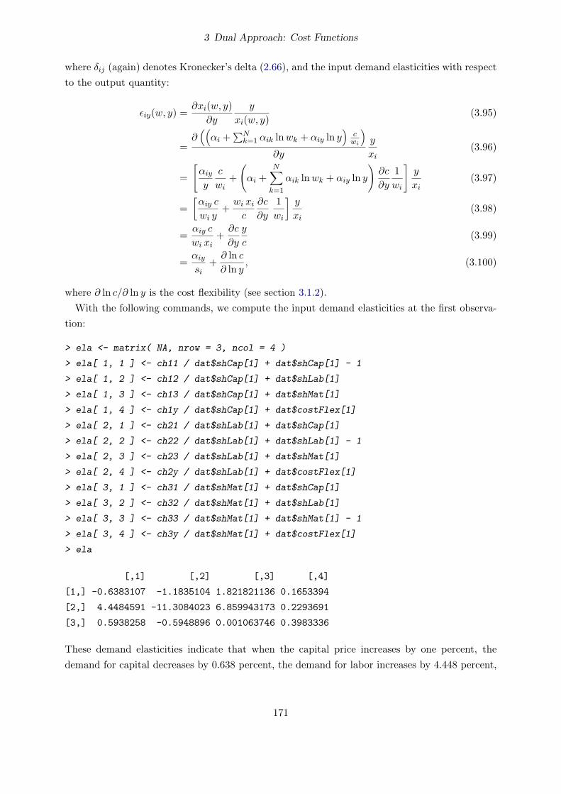
3 Dual Approach: Cost Functions
where δij (again) denotes Kronecker’s delta (2.66), and the input demand elasticities with respect
to the output quantity:
εiy(w, y) = ∂xi(w, y)∂y
y
xi(w, y) (3.95)
=∂((αi +
∑Nk=1 αik lnwk + αiy ln y
)cwi
)∂y
y
xi(3.96)
=[αiyy
c
wi+(αi +
N∑k=1
αik lnwk + αiy ln y)∂c
∂y
1wi
]y
xi(3.97)
=[αiy c
wi y+ wi xi
c
∂c
∂y
1wi
]y
xi(3.98)
= αiy c
wi xi+ ∂c
∂y
y
c(3.99)
= αiysi
+ ∂ ln c∂ ln y , (3.100)
where ∂ ln c/∂ ln y is the cost flexibility (see section 3.1.2).
With the following commands, we compute the input demand elasticities at the first observa-
tion:
> ela <- matrix( NA, nrow = 3, ncol = 4 )
> ela[ 1, 1 ] <- ch11 / dat$shCap[1] + dat$shCap[1] - 1
> ela[ 1, 2 ] <- ch12 / dat$shCap[1] + dat$shLab[1]
> ela[ 1, 3 ] <- ch13 / dat$shCap[1] + dat$shMat[1]
> ela[ 1, 4 ] <- ch1y / dat$shCap[1] + dat$costFlex[1]
> ela[ 2, 1 ] <- ch21 / dat$shLab[1] + dat$shCap[1]
> ela[ 2, 2 ] <- ch22 / dat$shLab[1] + dat$shLab[1] - 1
> ela[ 2, 3 ] <- ch23 / dat$shLab[1] + dat$shMat[1]
> ela[ 2, 4 ] <- ch2y / dat$shLab[1] + dat$costFlex[1]
> ela[ 3, 1 ] <- ch31 / dat$shMat[1] + dat$shCap[1]
> ela[ 3, 2 ] <- ch32 / dat$shMat[1] + dat$shLab[1]
> ela[ 3, 3 ] <- ch33 / dat$shMat[1] + dat$shMat[1] - 1
> ela[ 3, 4 ] <- ch3y / dat$shMat[1] + dat$costFlex[1]
> ela
[,1] [,2] [,3] [,4]
[1,] -0.6383107 -1.1835104 1.821821136 0.1653394
[2,] 4.4484591 -11.3084023 6.859943173 0.2293691
[3,] 0.5938258 -0.5948896 0.001063746 0.3983336
These demand elasticities indicate that when the capital price increases by one percent, the
demand for capital decreases by 0.638 percent, the demand for labor increases by 4.448 percent,
171

3 Dual Approach: Cost Functions
and the demand for materials increases by 0.594 percent. When the labor price increases by one
percent, the elasticities indicate that the demand for all inputs decreases, which is not possible
when the output quantity should be maintained. Furthermore, the symmetry condition for the
elasticities (3.54) indicates that the cross-price elasticities of each input pair must have the same
sign. However, this is not the case for the pairs capital–labor and materials–labor. The reason
for this is the negative predicted input share of labor:
> dat[ 1, c( "shCap", "shLab", "shMat" ) ]
shCap shLab shMat
1 0.2630271 -0.06997825 0.8069511
Finally, the negativity constraint (3.52) is violated, because the own-price elasticity of materials
is positive (0.001).
When the output quantity is increased by one percent, the demand for capital increases by
0.165 percent, the demand for labor increases by 0.229 percent, and the demand for materials
increases by 0.398 percent.
Now, we create a three-dimensional array and compute the demand elasticities for all observa-
tions:
> elaAll <- array( NA, c( 3, 4, nrow( dat ) ) )
> elaAll[ 1, 1, ] <- ch11 / dat$shCap + dat$shCap - 1
> elaAll[ 1, 2, ] <- ch12 / dat$shCap + dat$shLab
> elaAll[ 1, 3, ] <- ch13 / dat$shCap + dat$shMat
> elaAll[ 1, 4, ] <- ch1y / dat$shCap + dat$costFlex
> elaAll[ 2, 1, ] <- ch21 / dat$shLab + dat$shCap
> elaAll[ 2, 2, ] <- ch22 / dat$shLab + dat$shLab - 1
> elaAll[ 2, 3, ] <- ch23 / dat$shLab + dat$shMat
> elaAll[ 2, 4, ] <- ch2y / dat$shLab + dat$costFlex
> elaAll[ 3, 1, ] <- ch31 / dat$shMat + dat$shCap
> elaAll[ 3, 2, ] <- ch32 / dat$shMat + dat$shLab
> elaAll[ 3, 3, ] <- ch33 / dat$shMat + dat$shMat - 1
> elaAll[ 3, 4, ] <- ch3y / dat$shMat + dat$costFlex
We can visualize the elasticities using histograms but we will include only observations, at
which the cost function is non-decreasing in all input prices so that the optimal input shares are
always positive.
> monoObs <- with( dat, shCap >= 0 & shLab >= 0 & shMat >= 0 )
> hist( elaAll[1,1,monoObs] )
> hist( elaAll[1,2,monoObs] )
172

3 Dual Approach: Cost Functions
> hist( elaAll[1,3,monoObs] )
> hist( elaAll[2,1,monoObs] )
> hist( elaAll[2,2,monoObs] )
> hist( elaAll[2,3,monoObs] )
> hist( elaAll[3,1,monoObs] )
> hist( elaAll[3,2,monoObs] )
> hist( elaAll[3,3,monoObs] )
> hist( elaAll[1,4,monoObs] )
> hist( elaAll[2,4,monoObs] )
> hist( elaAll[3,4,monoObs] )
The resulting graphs are shown in figure 3.16. While the conditional own-price elasticities of
capital and materials are negative at almost all observations, the conditional own-price elasticity
of labor is positive at almost all observations. These violations of the negativity constraint (3.52)
originate from the violation of the concavity condition. As all conditional elasticities of the capital
demand with respect to the materials price as well as all conditional elasticities of the materials
demand with respect to the capital price are positive, we can conclude that capital and materials
are net substitutes. In contrast, all cross-price elasticities between capital and labor as well as
between labor and materials are negative. This indicates that the two pairs capital and labor as
well as labor and materials are net complements.
When the output quantity is increased by one percent, most farms would increase both the
labor quantity and the materials quantity by around 0.5% and either increase or decrease the
capital quantity.
3.4.9 Theoretical consistency
The Translog cost function (3.66) is always continuous for positive input prices and a positive
output quantity.
The non-negativity is always fulfilled for the Translog cost function, because the predicted cost
is equal to the exponential function of the right-hand side of equation (3.66) and the exponential
function always returns a non-negative value (also when the right-hand side of equation (3.66) is
negative).
If the output quantity approaches zero (from above), the right-hand side of the Translog cost
functions (equation 3.66) approaches:
limy→0+
α0 +N∑i=1
αi lnwi + αy ln y + 12
N∑i=1
N∑j=1
αij lnwi lnwj + 12αyy (ln y)2 +
N∑i=1
αiy lnwi ln y
(3.101)
= limy→0+
(αy ln y + 1
2αyy (ln y)2 +N∑i=1
αiy lnwi ln y)
(3.102)
173

3 Dual Approach: Cost Functions
E cap cap
Fre
quen
cy
0 5 10 15 20
020
4060
80
E cap lab
Fre
quen
cy
−300 −200 −100 0
020
4060
8010
0
E cap mat
Fre
quen
cy
0 50 100 150 200 250
020
4060
8010
0
E lab cap
Fre
quen
cy
−40 −30 −20 −10 0
020
4060
8010
0
E lab lab
Fre
quen
cy
0 20 40 60 80 100
020
4060
8010
0
E lab mat
Fre
quen
cy
−70 −50 −30 −10 0
020
4060
8010
0
E mat cap
Fre
quen
cy
0 1 2 3 4 5 6 7
020
4060
80
E mat lab
Fre
quen
cy
−8 −6 −4 −2 0
020
4060
8010
0
E mat mat
Fre
quen
cy
−0.5 0.5 1.5 2.5
020
4060
8010
0
E cap y
Fre
quen
cy
−40 −30 −20 −10 0
010
2030
4050
E lab y
Fre
quen
cy
0.0 0.5 1.0 1.5
010
2030
40
E mat y
Fre
quen
cy
0.0 0.4 0.8 1.2
010
2030
4050
Figure 3.16: Translog cost function: derived demand elasticities
174

3 Dual Approach: Cost Functions
= limy→0+
((αy + 1
2αyy ln y +N∑i=1
αiy lnwi
)ln y
)(3.103)
= limy→0+
(αy + 1
2αyy ln y +N∑i=1
αiy lnwi
)limy→0+
ln y (3.104)
= limy→0+
(αyy ln y) limy→0+
ln y = (−αyy∞)(−∞) = αyy∞ (3.105)
Hence, if coefficientt αyy is negativ and the output quantity approaches zero (from above), the
predicted cost (exponential function of the right-hand side of equation 3.66) approaches zero so
that the “no fixed costs” property is asymptotically fulfilled.
Our estimated Translog cost function with linear homogeneity in input prices imposed (of
course) is linearly homogeneous in input prices. Hence, the linear homogeneity property is globally
fulfilled.
A cost function is non-decreasing in the output quantity if the cost flexibility and the elasticity
of size are non-negative. As we can see from figure 3.7, only a single cost flexibility and thus,
only a single elasticity of size is negative. Hence, our estimated Translog cost function with linear
homogeneity in input prices imposed violates the monotonicity condition regarding the output
quantity only at a single observation.
Given Shepard’s lemma, a cost function is non-decreasing in input prices if the derived cost-
minimizing input quantities and the corresponding cost shares are non-negative. As we can see
from figure 3.13, our estimated Translog cost function with linear homogeneity in input prices
imposed predicts that 24 cost shares of capital, 10 cost shares of labor, and 3 cost shares of
materials are negative. In total, the monotonicity condition regarding the input prices is violated
at 36 observations:
> sum( dat$shCap < 0 | dat$shLab < 0 | dat$shMat < 0 )
[1] 36
Concavity in input prices of the cost function requires that the Hessian matrix of the cost
function with respect to the input prices is negative semidefinite. The elements of the Hessian
matrix are:
Hij = ∂2c(w, y)∂wi ∂wj
= ∂xi(w, y)∂wj
(3.106)
=∂((αi +
∑Nk=1 αik lnwk + αiy ln y
)cwi
)∂wj
(3.107)
= αijwj
c
wi+(αi +
N∑k=1
αik lnwk + αiy ln y)xjwi− δij
(αi +
N∑k=1
αik lnwk + αiy ln y)
c
w2i
(3.108)
= αij c
wiwj+ xiwi
c
xjwi− δij
xiwic
c
w2i
(3.109)
175
3 Dual Approach: Cost Functions
= αij c
wiwj+ xi xj
c− δij
xiwi, (3.110)
where δij (again) denotes Kronecker’s delta (2.66). As the elements of the Hessian matrix have
the same sign as the corresponding elasticities (Hij = εij(w, y) xi/wj), the positive own-price
elasticities of labor in figure 3.16 indicate that the element Hlab,lab is positive at all observa-
tions, where the monotonicity conditions regarding the input prices are fulfilled. As negative
semidefiniteness requires that all diagonal elements of the (Hessian) matrix are negative, we can
conclude that the estimated Translog cost function is concave at not a single observation where
the monotonicity conditions regarding the input prices are fulfilled.
This means that our estimated Translog cost function is inconsistent with microeconomic theory
at all observations.
176

4 Dual Approach: Profit Function
4.1 Theory
4.1.1 Profit functions
The profit function:
π(p, w) = maxy,x
p y −∑i
wi xi, s.t. y = f(x) (4.1)
returns the maximum profit that is attainable given the output price p and input prices w.
It is important to distinguish the profit definition (1.4) from the profit function (4.1).
4.1.2 Short-run profit functions
As producers often cannot instantly adjust the quantity of the some inputs (e.g. capital, land,
apple trees), estimating a short-run profit function with some quasi-fixed input quantities might
be more appropriate than a (long-run) profit function which assumes that all input quantities
and output quantities can be adjusted instantly. Furthermore, a short-run profit function can
model technologies with increasing returns to scale, if the sum over the output elasticities of the
variable inputs is lower than one.
In general, a short-run profit function is defined as
πv(p, w1, x2) = maxy≥0
{p y − cs(w1, y, x2)
}, (4.2)
where w1 denotes the vector of the prices of all variable inputs, x2 denotes the vector of the
quantities of all quasi-fixed inputs, cs(w1, y, x2) is the short-run cost function (see section 3.3),
πv denotes the gross margin defined in equation (1.5), and N1 is a vector of the indices of the
variable inputs.
4.2 Graphical illustration of profit and gross margin
We use the following commands to visualize the variation of the profits and the relationship
between profits and firm size:
> hist( dat$profit, 30 )
> plot( dat$X, dat$profit, log = "xy" )
177

4 Dual Approach: Profit Function
profit
Fre
quen
cy
0e+00 2e+07 4e+07 6e+07
020
4060
80
●
●
●
●
●
●●
●
●
●
●●
● ●
●
●
● ●●
●●
●
●
●
●●
●
●
●
●
●
●
●●
●
●
●
●
●● ●●●●
●●
●●●
●
●
●
●
●
●
●●
● ●
●
●
●
●
●
●
●
●
●
●
●● ●
● ●
●
●
●
●
●●
●●
●
●
●
●
●
● ●
●
●
●
●
●
●
●●
●●
●
●
●
●●
●
●
●
●
●
●
●
●
●
●
●
●
●
●
●
●
●
●
●
●
● ●
0.5 1.0 2.0 5.0
2e+
045e
+05
1e+
07
X
prof
it
Figure 4.1: Profit
The resulting graphs are shown in figure 4.1. The histogram shows that 14 out of 140 apple
producers (10%) have (slightly) negative profits. Although this seems to be not unrealistic, this
contradicts the non-negativity condition of the profit function. However, the observed negative
profits might have been caused by deviations from the theoretical assumptions that we have made
to derive the profit function, e.g. that all inputs can be instantly adjusted and that there are no
unexpected events such as severe weather conditions or pests. We will deal with these deviations
from our assumptions later and for now just ignore the observations with negative profits in
our analyses with the profit function. The right part of figure 4.1 shows that the profit clearly
increases with firm size.
The following commands graphically illustrate the variation of the gross margins and their
relationship to the firm size and the quantity of the quasi-fixed input:
> hist( dat$vProfit, 30 )
> plot( dat$X, dat$vProfit, log = "xy" )
> plot( dat$qCap, dat$vProfit, log = "xy" )
The resulting graphs are shown in figure 4.2. The histogram on the left shows that 8 out of
140 apple producers (6%) have (slightly) negative gross margins. Although this does not seem
to be unrealistic, this contradicts the non-negativity condition of the short-run profit function.
However, the observed negative gross margins might have been caused by deviations from the
theoretical assumptions, e.g. that there are no unexpected events such as severe weather condi-
tions or pests. The center part of figure 4.2 shows that the gross margin clearly increases with
the firm size (as expected). However, the right part of this figure shows that the gross margin is
only weakly positively correlated with the fixed input.
178
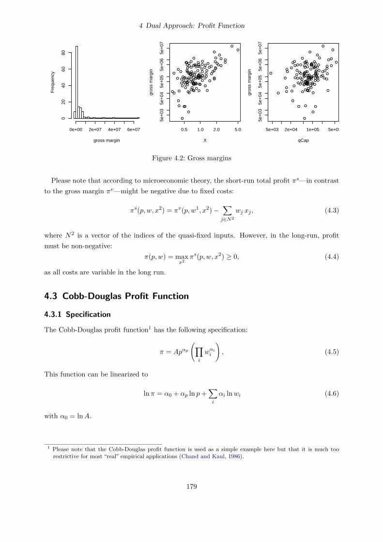
4 Dual Approach: Profit Function
gross margin
Fre
quen
cy
0e+00 2e+07 4e+07 6e+07
020
4060
80
●●
●
●
●
●●
●
●
●
●●
●●
●
●
●
●
● ●●
●●
●
●
●
●
●
●●
●
●
●
●
●
●●
●
●
●
●
●
●● ●●
●●
●●
●●●
●
●
●
●
●
●
●
●●
● ●
●
●
●
●
●
●
●
●
●
●
●
●●●
● ●
●
●
●
●
●●
●●
●
●
●
●
●
●●
●
●
●
●
●
●
●●
●●
●
●
●
●●
●
●
●
●
●
●
●
●
●
●
●
●
●
●
●
●
●
●
●
●
● ●
0.5 1.0 2.0 5.0
5e+
035e
+04
5e+
055e
+06
5e+
07
X
gros
s m
argi
n
●●
●
●
●
●●
●
●
●
●●
●●
●
●
●
●
● ●●
●●
●
●
●
●
●
●●
●
●
●
●
●
●●
●
●
●
●
●
●●●●
●●
●●
●●
●
●
●
●
●
●
●
●
●●
● ●
●
●
●
●
●
●
●
●
●
●
●
● ●●
● ●
●
●
●
●
●●
●●
●
●
●
●
●
●●
●
●
●
●
●
●
●●
●●
●
●
●
●●
●
●
●
●
●
●
●
●
●
●
●
●
●
●
●
●
●
●
●
●
● ●
5e+03 2e+04 1e+05 5e+05
5e+
035e
+04
5e+
055e
+06
5e+
07
qCap
gros
s m
argi
n
Figure 4.2: Gross margins
Please note that according to microeconomic theory, the short-run total profit πs—in contrast
to the gross margin πv—might be negative due to fixed costs:
πs(p, w, x2) = πv(p, w1, x2)−∑j∈N2
wj xj , (4.3)
where N2 is a vector of the indices of the quasi-fixed inputs. However, in the long-run, profit
must be non-negative:
π(p, w) = maxx2
πs(p, w, x2) ≥ 0, (4.4)
as all costs are variable in the long run.
4.3 Cobb-Douglas Profit Function
4.3.1 Specification
The Cobb-Douglas profit function1 has the following specification:
π = Apαp
(∏i
wαii
), (4.5)
This function can be linearized to
ln π = α0 + αp ln p+∑i
αi lnwi (4.6)
with α0 = lnA.
1 Please note that the Cobb-Douglas profit function is used as a simple example here but that it is much toorestrictive for most “real” empirical applications (Chand and Kaul, 1986).
179

4 Dual Approach: Profit Function
4.3.2 Estimation
The linearized Cobb-Douglas profit function can be estimated by OLS. As the logarithm of a
negative number is not defined and function lm automatically removes observations with missing
data, we do not have to remove the observations (apple producers) with negative profits manually.
> profitCD <- lm( log( profit ) ~ log( pOut ) + log( pCap ) + log( pLab ) +
+ log( pMat ), data = dat )
> summary( profitCD )
Call:
lm(formula = log(profit) ~ log(pOut) + log(pCap) + log(pLab) +
log(pMat), data = dat)
Residuals:
Min 1Q Median 3Q Max
-3.6183 -0.2778 0.1261 0.5986 2.0442
Coefficients:
Estimate Std. Error t value Pr(>|t|)
(Intercept) 13.9380 0.4921 28.321 < 2e-16 ***
log(pOut) 2.7117 0.2340 11.590 < 2e-16 ***
log(pCap) -0.7298 0.1752 -4.165 5.86e-05 ***
log(pLab) -0.1940 0.4623 -0.420 0.676
log(pMat) 0.1612 0.2543 0.634 0.527
---
Signif. codes: 0 ‘***’ 0.001 ‘**’ 0.01 ‘*’ 0.05 ‘.’ 0.1 ‘ ’ 1
Residual standard error: 0.9815 on 121 degrees of freedom
(14 observations deleted due to missingness)
Multiple R-squared: 0.5911, Adjusted R-squared: 0.5776
F-statistic: 43.73 on 4 and 121 DF, p-value: < 2.2e-16
As expected, lm reports that 14 observations have been removed due to missing data (logarithms
of negative numbers).
4.3.3 Properties
A Cobb-Douglas profit function is always continuous and twice continuously differentiable for all
p > 0 and wi > 0 ∀i. Furthermore, a Cobb-Douglas profit function automatically fulfills the
non-negativity property, because the profit predicted by equation (4.5) is always positive as long
as coefficient A is positive (given that all input prices and the output price are positive). As A
180

4 Dual Approach: Profit Function
is usually obtained by applying the exponential function to the estimate of α0, i.e. A = exp(α0),A and hence, also the predicted profit, are always positive (even if α0 is non-positive).
The estimated coefficients of the output price and the input prices indicate that profit is
increasing in the output price and decreasing in the capital and labor price but it is increasing in
the price of materials, which contradicts microeconomic theory. However, the positive coefficient
of the (logarithmic) price of materials is statistically not significantly different from zero.
The Cobb-Douglas profit function is linearly homogeneous in all prices (output price and all
input prices) if the following condition is fulfilled:
t π(p, w) = π(t p, t w) (4.7)
ln(t π) = α0 + αp ln(t p) +∑i
αi ln(t wi) (4.8)
ln t+ ln π = α0 + αp ln t+ αp ln p+∑i
αi ln t+∑i
αi lnwi (4.9)
ln t+ ln π = α0 + αp ln p+∑i
αi lnwi + ln t(αp +
∑i
αi
)(4.10)
ln π = ln π + ln t(αp +
∑i
αi − 1)
(4.11)
0 = ln t(αp +
∑i
αi − 1)
(4.12)
0 = αp +∑i
αi − 1 (4.13)
1 = αp +∑i
αi (4.14)
Hence, the homogeneity condition is only fulfilled if the coefficient of the (logarithmic) output
price and the coefficients of the (logarithmic) input prices sum up to one. As they sum up to
2.71+(−0.73)+(−0.19)+0.16 = 1.95, the homogeneity condition is not fulfilled in our estimated
model.
4.3.4 Estimation with linear homogeneity in all prices imposed
In order to derive a Cobb-Douglas profit function with linear homogeneity in input prices imposed,
we re-arrange the homogeneity condition (4.14) to get
αp = 1−N∑i=1
αi (4.15)
and replace αp in the profit function (4.6) by the right-hand side of the above equation:
ln π = α0 +(
1−∑i
αi
)ln p+
∑i
αi lnwi (4.16)
181

4 Dual Approach: Profit Function
ln π = α0 + ln p−∑i
αi ln p+∑i
αi lnwi (4.17)
ln π − ln p = α0 +∑i
αi (lnwi − ln p) (4.18)
ln πp
= α0 +∑i
αi ln wip
(4.19)
This Cobb-Douglas profit function with linear homogeneity imposed can be estimated by following
command:
> profitCDHom <- lm( log( profit / pOut ) ~ log( pCap / pOut ) +
+ log( pLab / pOut ) + log( pMat / pOut ), data = dat )
> summary( profitCDHom )
Call:
lm(formula = log(profit/pOut) ~ log(pCap/pOut) + log(pLab/pOut) +
log(pMat/pOut), data = dat)
Residuals:
Min 1Q Median 3Q Max
-3.6045 -0.2724 0.0972 0.6013 2.0385
Coefficients:
Estimate Std. Error t value Pr(>|t|)
(Intercept) 14.27961 0.45962 31.068 < 2e-16 ***
log(pCap/pOut) -0.82114 0.16953 -4.844 3.78e-06 ***
log(pLab/pOut) -0.90068 0.25591 -3.519 0.000609 ***
log(pMat/pOut) -0.02469 0.23530 -0.105 0.916610
---
Signif. codes: 0 ‘***’ 0.001 ‘**’ 0.01 ‘*’ 0.05 ‘.’ 0.1 ‘ ’ 1
Residual standard error: 0.9909 on 122 degrees of freedom
(14 observations deleted due to missingness)
Multiple R-squared: 0.3568, Adjusted R-squared: 0.341
F-statistic: 22.56 on 3 and 122 DF, p-value: 1.091e-11
The coefficient of the (logarithmic) output price can be obtained by the homogeneity restric-
tion (4.15). Hence, it is 1− (−0.82)− (−0.9)− (−0.02) = 2.75. Now, all monotonicity conditions
are fulfilled: profit is increasing in the output price and decreasing in all input prices. We can
use a Wald test or a likelihood-ratio test to test whether the model and the data contradict the
homogeneity assumption:
182

4 Dual Approach: Profit Function
> library( "car" )
> linearHypothesis( profitCD, "log(pOut) + log(pCap) + log(pLab) + log(pMat) = 1" )
Linear hypothesis test
Hypothesis:
log(pOut) + log(pCap) + log(pLab) + log(pMat) = 1
Model 1: restricted model
Model 2: log(profit) ~ log(pOut) + log(pCap) + log(pLab) + log(pMat)
Res.Df RSS Df Sum of Sq F Pr(>F)
1 122 119.78
2 121 116.57 1 3.2183 3.3407 0.07005 .
---
Signif. codes: 0 ‘***’ 0.001 ‘**’ 0.01 ‘*’ 0.05 ‘.’ 0.1 ‘ ’ 1
> lrtest( profitCD, profitCDHom )
Likelihood ratio test
Model 1: log(profit) ~ log(pOut) + log(pCap) + log(pLab) + log(pMat)
Model 2: log(profit/pOut) ~ log(pCap/pOut) + log(pLab/pOut) + log(pMat/pOut)
#Df LogLik Df Chisq Pr(>Chisq)
1 6 -173.88
2 5 -175.60 -1 3.4316 0.06396 .
---
Signif. codes: 0 ‘***’ 0.001 ‘**’ 0.01 ‘*’ 0.05 ‘.’ 0.1 ‘ ’ 1
Both tests reject the null hypothesis, linear homogeneity in all prices, at the 10% significance
level but not at the 5% level. Given the importance of microeconomic consistency and that 5%
is the standard significance level, we continue our analysis with the Cobb-Douglas profit function
with linear homogeneity imposed.
4.3.5 Checking Convexity in all prices
The last property that we have to check is the convexity in all prices. A continuous and twice
continuously differentiable function is convex, if its Hessian matrix is positive semidefinite. A
necessary condition for positive semidefiniteness is that all diagonal elements are non-negative,
while a sufficient condition is that all principal minors are non-negative (e.g. Chiang, 1984). The
183

4 Dual Approach: Profit Function
first derivatives of the Cobb-Douglas profit function with respect to the input prices are:
∂π
∂wi= ∂ ln π∂ lnwi
π
wi= αi
π
wi(4.20)
and the first derivative with respect to the output price is:
∂π
∂p= ∂ ln π∂ ln p
π
p= αp
π
p(4.21)
Now, we can calculate the second derivatives as derivatives of the first derivatives (4.20)
and (4.21):
∂2π
∂wi ∂wj=∂ ∂π∂wi
∂wj=∂(αi
πwi
)∂wj
(4.22)
= αiwi
∂π
∂wj− δij αi
π
w2i
(4.23)
= αiwiαj
π
wj− δij αi
π
w2i
(4.24)
= αi(αj − δij)π
wi wj(4.25)
∂2π
∂wi ∂p=∂ ∂π∂wi
∂p=∂(αi
πwi
)∂p
(4.26)
= αiwi
∂π
∂p(4.27)
= αiwiαpπ
p(4.28)
= αiαpπ
wi p(4.29)
∂2π
∂p2 =∂ ∂π∂p∂p
=∂(αp
πp
)∂p
(4.30)
= αpp
∂π
∂p− αp
π
p2 (4.31)
= αppαpπ
p− αp
π
p2 (4.32)
= αp(αp − 1) πp2 , (4.33)
where δij (again) denotes Kronecker’s delta (2.66).
As all elements of the Hessian matrix include π as a multiplicative term, we can ignore this
variable in the calculation of the Hessian matrix, because the value π neither changes the signs of
the (diagonal) elements of the matrix, nor the signs of the principal minors and the determinant
(as long as π is positive, i.e. the non-negativity condition is fulfilled) given the general rule that
|π ·M | = π · |M |, where M denotes a quadratic matrix, π denotes a scalar, and the two vertical
bars denote the determinant function.
184

4 Dual Approach: Profit Function
We start with checking convexity in all prices of the Cobb-Douglas profit function without
homogeneity imposed.
To simplify the calculations, we define short-cuts for the coefficients:
> gCap <- coef( profitCD )[ "log(pCap)" ]
> gLab <- coef( profitCD )[ "log(pLab)" ]
> gMat <- coef( profitCD )[ "log(pMat)" ]
> gOut <- coef( profitCD )[ "log(pOut)" ]
Using these coefficients, we compute the second derivatives of our estimated Cobb-Douglas profit
function:
> hpCapCap <- gCap * ( gCap - 1 ) / dat$pCap^2
> hpLabLab <- gLab * ( gLab - 1 ) / dat$pLab^2
> hpMatMat <- gMat * ( gMat - 1 ) / dat$pMat^2
> hpCapLab <- gCap * gLab / ( dat$pCap * dat$pLab )
> hpCapMat <- gCap * gMat / ( dat$pCap * dat$pMat )
> hpLabMat <- gLab * gMat / ( dat$pLab * dat$pMat )
> hpCapOut <- gCap * gOut / ( dat$pCap * dat$pOut )
> hpLabOut <- gLab * gOut / ( dat$pLab * dat$pOut )
> hpMatOut <- gMat * gOut / ( dat$pMat * dat$pOut )
> hpOutOut <- gOut * ( gOut - 1 ) / dat$pOut^2
Now, we prepare the Hessian matrix for the first observation:
> hessian <- matrix( NA, nrow = 4, ncol = 4 )
> hessian[ 1, 1 ] <- hpCapCap[1]
> hessian[ 2, 2 ] <- hpLabLab[1]
> hessian[ 3, 3 ] <- hpMatMat[1]
> hessian[ 1, 2 ] <- hessian[ 2, 1 ] <- hpCapLab[1]
> hessian[ 1, 3 ] <- hessian[ 3, 1 ] <- hpCapMat[1]
> hessian[ 2, 3 ] <- hessian[ 3, 2 ] <- hpLabMat[1]
> hessian[ 1, 4 ] <- hessian[ 4, 1 ] <- hpCapOut[1]
> hessian[ 2, 4 ] <- hessian[ 4, 2 ] <- hpLabOut[1]
> hessian[ 3, 4 ] <- hessian[ 4, 3 ] <- hpMatOut[1]
> hessian[ 4, 4 ] <- hpOutOut[1]
> print( hessian )
[,1] [,2] [,3] [,4]
[1,] 0.185633270 0.060331020 -0.005072286 -1.14920901
[2,] 0.060331020 0.286060178 -0.003907371 -0.88527867
[3,] -0.005072286 -0.003907371 -0.001709437 0.07442915
[4,] -1.149209014 -0.885278673 0.074429148 10.64451706
185

4 Dual Approach: Profit Function
As the third element on the diagonal of this Hessian matrix is negative, the necessary condition
for positive semidefiniteness is not fulfilled. Hence, we do not need to calculate the principal
minors of the Hessian matrix, as we already can conclude that the Hessian matrix is not positive
semidefinite and hence, the estimated profit function is not convex at the first observation.2
We can check whether the third element on the diagonal of the Hessian matrix is non-negative
at other observations:
> sum( hpMatMat >= 0, na.rm = TRUE )
[1] 0
As it is non-negative not at a single observation, we must conclude that the estimated Cobb-
Douglas profit function without homogeneity imposed violates the convexity property at all ob-
servations.
Now, we will check, whether our Cobb-Douglas profit function with linear homogeneity imposed
is convex in all prices. Again, we create short-cuts for the estimated coefficients:
> ghCap <- coef( profitCDHom )["log(pCap/pOut)"]
> ghLab <- coef( profitCDHom )["log(pLab/pOut)"]
> ghMat <- coef( profitCDHom )["log(pMat/pOut)"]
> ghOut <- 1- ghCap - ghLab - ghMat
We compute the second derivatives:
> hphCapCap <- ghCap * ( ghCap - 1 ) / dat$pCap^2
> hphLabLab <- ghLab * ( ghLab - 1 ) / dat$pLab^2
> hphMatMat <- ghMat * ( ghMat - 1 ) / dat$pMat^2
> hphCapLab <- ghCap * ghLab / ( dat$pCap * dat$pLab )
> hphCapMat <- ghCap * ghMat / ( dat$pCap * dat$pMat )
> hphLabMat <- ghLab * ghMat / ( dat$pLab * dat$pMat )
> hphCapOut <- ghCap * ghOut / ( dat$pCap * dat$pOut )
> hphLabOut <- ghLab * ghOut / ( dat$pLab * dat$pOut )
> hphMatOut <- ghMat * ghOut / ( dat$pMat * dat$pOut )
> hphOutOut <- ghOut * ( ghOut - 1 ) / dat$pOut^2
And we prepare the Hessian matrix for the first observation:
> hessianHom <- matrix( NA, nrow = 4, ncol = 4 )
> hessianHom[ 1, 1 ] <- hphCapCap[1]
> hessianHom[ 2, 2 ] <- hphLabLab[1]
> hessianHom[ 3, 3 ] <- hphMatMat[1]
2 Please note that this Hessian matrix is not negative semidefinite either, because the other three principal minorsare positive. Hence, the Cobb-Douglas profit function is neither concave nor convex at the first observation.
186

4 Dual Approach: Profit Function
> hessianHom[ 1, 2 ] <- hessianHom[ 2, 1 ] <- hphCapLab[1]
> hessianHom[ 1, 3 ] <- hessianHom[ 3, 1 ] <- hphCapMat[1]
> hessianHom[ 2, 3 ] <- hessianHom[ 3, 2 ] <- hphLabMat[1]
> hessianHom[ 1, 4 ] <- hessianHom[ 4, 1 ] <- hphCapOut[1]
> hessianHom[ 2, 4 ] <- hessianHom[ 4, 2 ] <- hphLabOut[1]
> hessianHom[ 3, 4 ] <- hessianHom[ 4, 3 ] <- hphMatOut[1]
> hessianHom[ 4, 4 ] <- hphOutOut[1]
> print( hessianHom )
[,1] [,2] [,3] [,4]
[1,] 0.2198994186 0.315188197 0.0008740851 -1.30964735
[2,] 0.3151881974 2.114366248 0.0027786041 -4.16320062
[3,] 0.0008740851 0.002778604 0.0003198275 -0.01154546
[4,] -1.3096473550 -4.163200623 -0.0115454561 11.00022565
As all diagonal elements of this Hessian matrix are positive, the necessary conditions for posi-
tive semidefiniteness are fulfilled. Now, we calculate the principal minors in order to check the
sufficient conditions for positive semidefiniteness:
> hessianHom[1,1]
[1] 0.2198994
> det( hessianHom[1:2,1:2] )
[1] 0.3656043
> det( hessianHom[1:3,1:3] )
[1] 0.0001151481
> det( hessianHom )
[1] -1.129906e-19
The conditions for the first three principal minors are fulfilled and the fourth principal minor is
close to zero, where it is positive on some computers but negative on other computers. As Hessian
matrices of linear homogeneous functions are always singular, it is expected that the determinant
of the Hessian matrix (the Nth principal minor) is zero. However, the computed determinant
of our Hessian matrix is not exactly zero due to rounding errors, which are unavoidable on
digital computers. Given that the determinant of the Hessian matrix of our Cobb-Douglas cost
function with linear homogeneity imposed should always be zero, the Nth sufficient condition for
positive semidefiniteness (sign of the determinant of the Hessian matrix) should always be fulfilled.
187
4 Dual Approach: Profit Function
Consequently, we can conclude that our Cobb-Douglas profit function with linear homogeneity
imposed is convex in all prices at the first observation. In order to avoid problems due to rounding
errors, we can just check the positive semidefiniteness of the first N − 1 rows and columns of the
Hessian matrix:
> semidefiniteness( hessianHom[1:3,1:3], positive = TRUE )
[1] TRUE
In the following, we will check whether convexity in all prices is fulfilled at each observation in
the sample:
> dat$convexCDHom <- NA
> for( obs in 1:nrow( dat ) ) {
+ hessianPart <- matrix( NA, nrow = 3, ncol = 3 )
+ hessianPart[ 1, 1 ] <- hphCapCap[obs]
+ hessianPart[ 2, 2 ] <- hphLabLab[obs]
+ hessianPart[ 3, 3 ] <- hphMatMat[obs]
+ hessianPart[ 1, 2 ] <- hessianPart[ 2, 1 ] <- hphCapLab[obs]
+ hessianPart[ 1, 3 ] <- hessianPart[ 3, 1 ] <- hphCapMat[obs]
+ hessianPart[ 2, 3 ] <- hessianPart[ 3, 2 ] <- hphLabMat[obs]
+ dat$convexCDHom[obs] <-
+ semidefiniteness( hessianPart, positive = TRUE )
+ }
> sum( !dat$convexCDHom, na.rm = TRUE )
[1] 0
This result indicates that the convexity condition is violated not at a single observation. Conse-
quently, our Cobb-Douglas profit function with linear homogeneity imposed is convex in all prices
at all observations.
4.3.6 Predicted profit
As the dependent variable of the Cobb-Douglas profit function without homogeneity imposed is
ln(π), we have to apply the exponential function to the fitted dependent variable, in order obtain
the fitted profit π. Furthermore, we have to be aware of that the fitted method only returns
the predicted values for the observations that were included in the estimation. Hence, we have
to make sure that the predicted profits are only assigned to the observations that have a positive
profit and hence, were included in the estimation:
> dat$profitCD[ dat$profit > 0 ] <- exp( fitted( profitCD ) )
188

4 Dual Approach: Profit Function
We obtain the predicted profit from the Cobb-Douglas profit function with homogeneity im-
posed by:
> dat$profitCDHom[ dat$profit > 0 ] <- exp( fitted( profitCDHom ) ) * dat$pOut
4.3.7 Optimal Profit Shares
Given Hotelling’s Lemma, the coefficients of the (logarithmic) output price and the (logarithmic)
input prices are equal to the optimal “profit shares” derived from a Cobb-Douglas profit function:
αp = ∂ ln π(p, w)∂ ln p = ∂π(p, w)
∂p
p
π(p, w) = y(p, w) p
π(p, w) = p y(p, w)π(w, y) ≡ r(p, w) ≥ 1 (4.34)
αi = ∂ ln π(p, w)∂ lnwi
= ∂π(p, w)∂wi
wiπ(p, w) = −xi(p, w) wi
π(p, w) = −wi xi(p, w)π(w, y) ≡ ri(p, w) ≤ 0 (4.35)
In contrast to “real” shares, these “profit shares” are never between zero and one but they sum
up to one, as do “real” shares:
r +∑i
ri = p y
π+∑i
(−wi xi
π
)= p y −
∑iwi xi
π= π
π= 1 (4.36)
For instance, an optimal profit share of the output of αp = 2.75 means that profit maximization
would result in a total revenue that is 2.75 times as large as the profit, which corresponds to
a return on sales of 1/2.75 = 36%. Similarly, an optimal profit share of the capital input of
αcap = −0.82 means that profit maximization would result in total capital costs that are 0.82
times as large as the profit.
The following commands draw histograms of the observed profit shares and compare them to
the optimal profit shares, which are predicted by our Cobb-Douglas profit function with linear
homogeneity imposed:
> hist( ( dat$pOut * dat$qOut / dat$profit )[
+ dat$profit > 0 ], 30 )
> lines( rep( ghOut, 2), c( 0, 100 ), lwd = 3 )
> hist( ( - dat$pCap * dat$qCap / dat$profit )[
+ dat$profit > 0 ], 30 )
> lines( rep( ghCap, 2), c( 0, 100 ), lwd = 3 )
> hist( ( - dat$pLab * dat$qLab / dat$profit )[
+ dat$profit > 0 ], 30 )
> lines( rep( ghLab, 2), c( 0, 100 ), lwd = 3 )
> hist( ( - dat$pMat * dat$qMat / dat$profit )[
+ dat$profit > 0 ], 30 )
> lines( rep( ghMat, 2), c( 0, 100 ), lwd = 3 )
The resulting graphs are shown in figure 4.3. These results somewhat contradict previous results.
189

4 Dual Approach: Profit Function
profit share out
Fre
quen
cy
5 10 15 20
020
4060
80
profit share cap
Fre
quen
cy
−6 −5 −4 −3 −2 −1 00
2040
6080
profit share lab
Fre
quen
cy
−6 −4 −2 0
020
4060
profit share mat
Fre
quen
cy
−5 −4 −3 −2 −1 0
020
4060
80
Figure 4.3: Cobb-Douglas profit function: observed and optimal profit shares
190

4 Dual Approach: Profit Function
While the results based on production functions and cost functions indicate that the apple pro-
ducers on average use too much capital and too few materials, the results of the Cobb-Douglas
profit function indicate that almost all apple producers use too much materials and most apple
producers use too less capital and labor. However, the results of the Cobb-Douglas profit function
are consistent with previous results regarding the output quantity: all results suggest that most
apple producers should produce more output.
4.3.8 Derived Output Supply Input Demand Functions
Hotelling’s Lemma says that the partial derivative of a profit function with respect to the output
price is the output supply function and that the partial derivatives of a profit function with
respect to the input prices are the negative (unconditional) input demand functions:
y(p, w) = ∂π(p, w)∂p
= αpπ(p, w)p
(4.37)
xi(p, w) = −∂π(p, w)∂wi
= −αiπ(p, w)wi
(4.38)
These output supply and input demand functions should be homogeneous of degree zero in all
prices:
y(t p, t w) = y(p, w) (4.39)
xi(t p, t w) = xi(p, w) (4.40)
This condition is fulfilled for the output supply and input demand functions derived from a
linearly homogeneous Cobb-Douglas profit function:
y(t p, t w) = αpπ(t p, t w)
t p= αp
t π(p, w)t p
= αpπ(p, w)p
= y(p, w) (4.41)
xi(t p, t w) = −αiπ(t p, t w)
t wi= −αi
t π(p, w)t wi
= −αiπ(p, w)wi
= xi(p, w) (4.42)
4.3.9 Derived Output Supply and Input Demand Elasticities
Based on the derived output supply function (4.37) and the derived input demand functions (4.38),
we can derive the output supply elasticities and the (unconditional) input demand elasticities:
εyp(p, w) = ∂y(p, w)∂p
p
y(p, w) (4.43)
= αpp
∂π(p, w)∂p
p
y(p, w) − αpπ(p, w)p2
p
y(p, w) (4.44)
= αppy(p, w) p
y(p, w) − αpπ(p, w)p y(p, w) (4.45)
= αp −αp
r(w, y) (4.46)
191

4 Dual Approach: Profit Function
= αp − 1 (4.47)
εyj(p, w) = ∂y(p, w)∂wj
wjy(p, w) (4.48)
= αpp
∂π(p, w)∂wj
wjy(p, w) (4.49)
= −αppxj(p, w) wj
y(p, w) (4.50)
= −αpπ(p, w)p y(p, w)
wj xj(p, w)π(p, w) (4.51)
= αp rj(w, y)r(w, y) (4.52)
= αj (4.53)
εip(p, w) = ∂xi(p, w)∂p
p
xi(p, w) (4.54)
= −αiwi
∂π(p, w)∂p
p
xi(p, w) (4.55)
= −αiwi
y(p, w) p
xi(p, w) (4.56)
= −αiπ(p, w)
wi xi(p, w)p y(p, w)π(p, w) (4.57)
= αi αpri(w, y) (4.58)
= αp (4.59)
εij(p, w) = ∂xi(p, w)∂wj
wjxi(p, w) (4.60)
= −αiwi
∂π(p, w)∂wj
wjxi(p, w) + δij αi
π(p, w)w2j
wjxi(p, w) (4.61)
= αiwi
xj(p, w) wjxi(p, w) + δij αi
π(p, w)wi xi(p, w) (4.62)
= αiπ(p, w)
wi xi(p, w)wjxj(p, w)π(p, w) − δij
αiri(w, y) (4.63)
= αi rj(w, y)ri(w, y) − δij
αiri(w, y) (4.64)
= αj − δij (4.65)
All derived input demand elasticities based on our Cobb-Douglas profit function with linear
192

4 Dual Approach: Profit Function
homogeneity imposed are presented in table 4.1. If the output price increases by one percent, the
profit-maximizing firm will increase the use of capital, labor, and materials by 2.75% each, which
increases the production by 1.75%. The proportional increase of the input quantities (+2.75%)
results in a less than proportional increase in the output quantity (+1.75%). This indicates
that the model exhibits decreasing returns to scale, which is not surprising, because a profit
maximum cannot be in an area of increasing returns to scale (if all inputs are variable and all
markets function perfectly). If the price of capital increases by one percent, the profit-maximizing
firm will decrease the use of capital by 1.82% and decrease the use of labor and materials by 0.82%
each, which decreases the production by 0.82%. If the price of labor increases by one percent,
the profit-maximizing firm will decrease the use of labor by 1.9% and decrease the use of capital
and materials by 0.9% each, which decreases the production by 0.9%. If the price of materials
increases by one percent, the profit-maximizing firm will decrease the use of materials by 1.02%
and decrease the use of capital and labor by 0.02% each, which will decrease the production by
0.02%.
Table 4.1: Output supply and input demand elasticities derived from Cobb-Douglas profit func-tion (with linear homogeneity imposed)
p wcap wlab wmaty 1.75 -0.82 -0.9 -0.02xcap 2.75 -1.82 -0.9 -0.02xlab 2.75 -0.82 -1.9 -0.02xmat 2.75 -0.82 -0.9 -1.02
4.4 Cobb-Douglas Short-Run Profit Function
4.4.1 Specification
The specification of a Cobb-Douglas short-run profit function is
πv = A pαp
∏i∈N1
wαii
∏j∈N2
xαjj
, (4.66)
This Cobb-Douglas short-run profit function can be linearized to
ln πv = α0 + αp ln p+∑i∈N1
αi lnwi +∑j∈N2
αj ln xj (4.67)
with α0 = lnA.
193

4 Dual Approach: Profit Function
4.4.2 Estimation
We can estimate a Cobb-Douglas short-run profit function with capital as a quasi-fixed input
using the following commands. Again, function lm automatically removes the observations (apple
producers) with negative gross margin:
> profitCDSR <- lm( log( vProfit ) ~ log( pOut ) + log( pLab ) + log( pMat ) +
+ log( qCap ), data = dat )
> summary( profitCDSR )
Call:
lm(formula = log(vProfit) ~ log(pOut) + log(pLab) + log(pMat) +
log(qCap), data = dat)
Residuals:
Min 1Q Median 3Q Max
-4.7422 -0.0646 0.2578 0.4931 0.8989
Coefficients:
Estimate Std. Error t value Pr(>|t|)
(Intercept) 3.2739 1.2261 2.670 0.008571 **
log(pOut) 3.1745 0.2263 14.025 < 2e-16 ***
log(pLab) -1.6188 0.4434 -3.651 0.000381 ***
log(pMat) -0.7637 0.2687 -2.842 0.005226 **
log(qCap) 1.0960 0.1245 8.802 8.31e-15 ***
---
Signif. codes: 0 ‘***’ 0.001 ‘**’ 0.01 ‘*’ 0.05 ‘.’ 0.1 ‘ ’ 1
Residual standard error: 0.9659 on 127 degrees of freedom
(8 observations deleted due to missingness)
Multiple R-squared: 0.6591, Adjusted R-squared: 0.6484
F-statistic: 61.4 on 4 and 127 DF, p-value: < 2.2e-16
4.4.3 Properties
This short-run profit function fulfills all microeconomic monotonicity conditions: it is increasing
in the output price, it is decreasing in the prices of all variable inputs, and it is increasing in the
quasi-fixed input quantity. However, the homogeneity condition is not fulfilled, as the coefficient
of the output price and the coefficients of the prices of the variable inputs do not sum up to one
but to 3.17 + (−1.62) + (−0.76) = 0.79.
194

4 Dual Approach: Profit Function
4.4.4 Estimation with linear homogeneity in all prices imposed
We can impose the homogeneity condition on the Cobb-Douglas short-run profit function using
the same method as for the Cobb-Douglas (long-run) profit function:
> profitCDSRHom <- lm( log( vProfit / pOut ) ~ log( pLab / pOut ) +
+ log( pMat / pOut ) + log( qCap ), data = dat )
> summary( profitCDSRHom )
Call:
lm(formula = log(vProfit/pOut) ~ log(pLab/pOut) + log(pMat/pOut) +
log(qCap), data = dat)
Residuals:
Min 1Q Median 3Q Max
-4.7302 -0.0677 0.2598 0.5160 0.8916
Coefficients:
Estimate Std. Error t value Pr(>|t|)
(Intercept) 3.3145 1.2184 2.720 0.00743 **
log(pLab/pOut) -1.4574 0.2252 -6.471 1.88e-09 ***
log(pMat/pOut) -0.7156 0.2427 -2.949 0.00380 **
log(qCap) 1.0847 0.1212 8.949 3.50e-15 ***
---
Signif. codes: 0 ‘***’ 0.001 ‘**’ 0.01 ‘*’ 0.05 ‘.’ 0.1 ‘ ’ 1
Residual standard error: 0.9628 on 128 degrees of freedom
(8 observations deleted due to missingness)
Multiple R-squared: 0.5227, Adjusted R-squared: 0.5115
F-statistic: 46.73 on 3 and 128 DF, p-value: < 2.2e-16
We can obtain the coefficient of the output price from the homogeneity condition (4.15): 1 −(−1.457) − (−0.716) = 3.173. All microeconomic monotonicity conditions are still fulfilled: the
Cobb-Douglas short-run profit function with homogeneity imposed is increasing in the output
price, decreasing in the prices of all variable inputs, and increasing in the quasi-fixed input
quantity.
We can test the homogeneity restriction by a likelihood ratio test:
> lrtest( profitCDSRHom, profitCDSR )
Likelihood ratio test
195

4 Dual Approach: Profit Function
Model 1: log(vProfit/pOut) ~ log(pLab/pOut) + log(pMat/pOut) + log(qCap)
Model 2: log(vProfit) ~ log(pOut) + log(pLab) + log(pMat) + log(qCap)
#Df LogLik Df Chisq Pr(>Chisq)
1 5 -180.27
2 6 -180.17 1 0.1859 0.6664
Given the large P -value, we can conclude that the data do not contradict the linear homogeneity
in the output price and the prices of the variable inputs.
4.4.5 Returns to scale
The sum over the coefficients of all quasi-fixed inputs indicates the percentage change of the gross
margin if the quantities of all quasi-fixed inputs are increased by one percent: If this sum is larger
than one, the increase in gross margin is more than proportional to the increase in the quasi-fixed
inputs. Hence, the technology has increasing returns to scale. If this sum over the coefficients of
all quasi-fixed inputs is smaller than one, the increase in gross margin is less than proportional
to the increase in the quasi-fixed inputs and the technology has decreasing returns to scale. As
the coefficient of our (single) quasi-fixed input is larger than one (1.085), we can conclude that
the technology has increasing returns to scale.
4.4.6 Shadow prices of quasi-fixed inputs
The partial derivatives of the short-run profit function with respect to the quantities of the
quasi-fixed inputs denote the additional gross margins that can be earned by an additional unit
of these quasi-fixed inputs. These internal marginal values of the quasi-fixed inputs are usually
called “shadow prices”. In case of the Cobb-Douglas short-run profit function, the shadow prices
can be computed by∂πv
∂xj= ∂ ln πv
∂ ln xjπv
xj= αj
πv
xj(4.68)
Before we can calculate the shadow price of the capital input, we need to calculate the predicted
gross margin πv. As the dependent variable of the Cobb-Douglas short-run profit function with
homogeneity imposed is ln(πv/ ln p), we have to apply the exponential function to the fitted
dependent variable and then we have to multiply the result with p, in order obtain the fitted
gross margins πv. Furthermore, we have to be aware of that the fitted method only returns
the predicted values for the observations that were included in the estimation. Hence, we have
to make sure that the predicted gross margins are only assigned to the observations that have a
positive gross margin and hence, were included in the estimation:
> dat$vProfitCDHom[ dat$vProfit > 0 ] <-
+ exp( fitted( profitCDSRHom ) ) * dat$pOut[ dat$vProfit > 0 ]
Now, we can calculate the shadow price of the capital input for each apple producer who has a
positive gross margin and hence, was included in the estimation:
196

4 Dual Approach: Profit Function
> dat$pCapShadow <- with( dat, coef(profitCDSRHom)["log(qCap)"] *
+ vProfitCDHom / qCap )
The following commands show the variation of the shadow prices of capital and compare them
to the observed capital prices:
> hist( dat$pCapShadow, 30 )
> hist( dat$pCapShadow[ dat$pCapShadow < 30 ], 30 )
> compPlot( dat$pCap, dat$pCapShadow, log = "xy" )
shadow price of capital
Fre
quen
cy
0 100 200 300 400
010
2030
4050
60
shadow price of capital
Fre
quen
cy
0 5 10 15 20 25 30
02
46
810
●
●
●
●
●
●●
●
●
●
●
●
●
●
●
●●
●
●
●
●
●
●
●●
● ●
● ●
●
●
●
●
●
●
●
●
●
●
●
●
●
●●●
●
●●●
●
●
●
●
●
●
●
●
●
●
●
●●
●
●
●
●
●
●●
●
●
●● ●
●
●●
●●●
●
●
●
●
●●
●
●
●
●
●●
●
●
●
●
●
●
●●●
●
●
●●
●
●
●
●
●
●●
●
●●
●
●
●
●
●
●
●
●
●
●
●
●●
●
●
●
●
0.2 1.0 5.0 20.0 200.0
0.2
1.0
5.0
50.0
500.
0
observed prices
shad
ow p
rices
Figure 4.4: Shadow prices of capital
The resulting graphs are shown in figure 4.4. The two histograms show that most shadow prices
are below 30 and many shadow prices are between 3 and 11 but there are also some apple
producers who would gain much more from increasing their capital input. Indeed, all apple
producers have a higher shadow price of capital than the observed price of capital, where the
difference is small for some producers and large for other producers. These differences can be
explained by risk aversion and market failures on the credit market or land market (e.g. marginal
prices are not equal to average prices).
197

5 Stochastic Frontier Analysis
5.1 Theory
5.1.1 Different Efficiency Measures
5.1.1.1 Output-Oriented Technical Efficiency with One Output
The output-oriented technical efficiency according to Shepard is defined as
TE = y
y∗⇔ y = TE · y∗ 0 ≤ TE ≤ 1, (5.1)
where y is the observed output quantity and y∗ is the maximum output quantity that can be
produced with the observed input quantities x.
The output-oriented technical efficiency according to Farrell is defined as
TE = y∗
y⇔ y∗ = TE · y TE ≥ 1. (5.2)
These efficiency measures are graphically illustrated in Bogetoft and Otto (2011, p. 26, fig-
ure 2.2).
5.1.1.2 Input-Oriented Technical Efficiency with One Input
The input-oriented technical efficiency according to Shepard is defined as
TE = x
x∗⇔ x = TE · x∗ TE ≥ 1, (5.3)
where x is the observed input quantity and x∗ is the minimum input quantity at which the
observed output quantities y can be produced.
The input-oriented technical efficiency according to Farrell is defined as
TE = x∗
x⇔ x∗ = TE · x 0 ≤ TE ≤ 1. (5.4)
These efficiency measures are graphically illustrated in Bogetoft and Otto (2011, p. 26, fig-
ure 2.2).
198

5 Stochastic Frontier Analysis
5.1.1.3 Output-Oriented Technical Efficiency with Two or More Outputs
The output-oriented technical efficiencies according to Shepard and Farrell assume a proportional
increase of all output quantities, while all input quantities are held constant.
Hence, the output-oriented technical efficiency according to Shepard is defined as
TE = y1y∗1
= y2y∗2
= . . . = yMy∗M
⇔ yi = TE · y∗i ∀ i 0 ≤ TE ≤ 1, (5.5)
where y1, y2, . . . , yM are the observed output quantities, y∗1, y∗2, . . . , y∗M are the maximum output
quantities (given a proportional increase of all output quantities) that can be produced with the
observed input quantities x, and M is the number of outputs.
The output-oriented technical efficiency according to Farrell is defined as
TE = y∗1y1
= y∗2y2
= . . . = y∗MyM
⇔ y∗i = TE · yi ∀ i TE ≥ 1. (5.6)
These efficiency measures are graphically illustrated in Bogetoft and Otto (2011, p. 27, fig-
ure 2.3, right panel).
5.1.1.4 Input-Oriented Technical Efficiency with Two or More Inputs
The input-oriented technical efficiencies according to Shepard and Farrell assume a proportional
reduction of all inputs, while all outputs are held constant.
Hence, the input-oriented technical efficiency according to Shepard is defined as
TE = x1x∗1
= x2x∗2
= . . . = xNx∗N
⇔ xi = TE · x∗i ∀ i TE ≥ 1 (5.7)
where x1, x2, . . . , xN are the observed input quantities, x∗1, x∗2, . . . , x∗N are the minimum input
quantities (given a proportional decrease of all input quantities) at which the observed output
quantities y can be produced, and N is the number of inputs.
The input-oriented technical efficiency according to Farrell is defined as
TE = x∗1x1
= x∗2x2
= . . . = x∗NxN
⇔ x∗i = TE · xi ∀ i 0 ≤ TE ≤ 1. (5.8)
These efficiency measures are graphically illustrated in Bogetoft and Otto (2011, p. 27, fig-
ure 2.3, left panel).
5.1.1.5 Output-Oriented Allocative Efficiency and Revenue Efficiency
According to equation (5.6), the output-oriented technical efficiency according to Farrell is
TE = y1y1
= y2y2
= . . . = yMyM
= p y
p y, (5.9)
199

5 Stochastic Frontier Analysis
where y is the vector of technically efficient output quantities and p is the vector of output prices.
The output-oriented allocative efficiency according to Farrell is defined as
AE = p y∗
p y= p y
p y, (5.10)
where y∗ is the vector of technically efficient and allocatively efficient output quantities and y is
the vector of output quantities so that p y = p y∗ and yi/yi = AE ∀ i.Finally, the revenue efficiency according to Farrell is
RE = p y∗
p y= p y∗
p y
p y
p y= AE · TE (5.11)
All these efficiency measures can also be specified according to Shepard by just taking the in-
verse of the Farrell specifications. These efficiency measures are graphically illustrated in Bogetoft
and Otto (2011, p. 40, figure 2.11).
5.1.1.6 Input-Oriented Allocative Efficiency and Cost Efficiency
According to equation (5.8), the input-oriented technical efficiency according to Farrell is
TE = x1x1
= x2x2
= . . . = xNxN
= w x
w x, (5.12)
where x is the vector of technically efficient input quantities and w is the vector of output prices.
The input-oriented allocative efficiency according to Farrell is defined as
AE = w x∗
w x= w x
w x, (5.13)
where x∗ is the vector of technically efficient and allocatively efficient input quantities and x is
the vector of output quantities so that w x = w x∗ and xi/xi = AE ∀ i.Finally, the cost efficiency according to Farrell is
CE = w x∗
w x= w x∗
w x
w x
w x= AE · TE (5.14)
All these efficiency measures can also be specified according to Shepard by just taking the in-
verse of the Farrell specifications. These efficiency measures are graphically illustrated in Bogetoft
and Otto (2011, p. 36, figure 2.9).
5.1.1.7 Profit Efficiency
The profit efficiency according to Farrell is defined as
PE = p y∗ − w x∗
p y − w x, (5.15)
200
5 Stochastic Frontier Analysis
where y∗ and x∗ denote the profit maximizing output quantities and input quantities, respectively
(assuming full technical efficiency). The profit efficiency according to Shepard is just the inverse
of the Farrell specifications.
5.1.1.8 Scale efficiency
In case of one input x and one output y = f(x), the scale efficiency according to Farrell is defined
as
SE = AP ∗
AP, (5.16)
where AP = f(x)/x is the observed average product AP ∗ = f(x∗)/x∗ is the maximum average
product, and x∗ is the input quantity that results in the maximum average product.
The first-order condition for a maximum of the average product is
∂AP
∂x= ∂f(x)
∂x
1x− f(x)
x2 = 0 (5.17)
This condition can be re-arranged to
∂f(x)∂x
x
f(x) = 1 (5.18)
Hence, a necessary (but not sufficient) condition for a maximum of the average product is an
elasticity of scale equal to one.
5.2 Stochastic Production Frontiers
5.2.1 Specification
In section 2, we have estimated average production functions, where about half of the observations
were below the estimated production function and about half of the observations were above the
estimated production function (see left panel of figure 5.1). However, in microeconomic theory,
the production function indicates the maximum output quantity for each given set of input
quantities. Hence, theoretically, no observation could be above the production function and an
observations below the production function would indicate technical inefficiency.
This means that all residuals must be negative or zero. A production function with only
non-positive residuals could look like:
ln y = ln f(x)− u with u ≥ 0, (5.19)
where −u ≤ 0 are the non-positive residuals. One solution to achieve this could be to estimate
an average production function by ordinary least squares and then simply shift the production
function up until all residuals are negative or zero (see right panel of figure 5.1). However, this
201

5 Stochastic Frontier Analysis
y
x
oo
o
o
o
o
o
oo
o
o o
o
oo
o
o
o
y
x
oo
o
o
o
o
o
oo
o
o o
o
oo
o
o
o
Source: Bogetoft and Otto (2011)
Figure 5.1: Production function estimation: ordinary regression and with intercept correction
procedure does not account for statistical noise and is very sensitive to positive outliers.1 As
virtually all data sets and models are flawed with statistical noise, e.g. due to measurement
errors, omitted variables, and approximation errors, Meeusen and van den Broeck (1977) and
Aigner, Lovell, and Schmidt (1977) independently proposed the stochastic frontier model that
simultaneously accounts for statistical noise and technical inefficiency:
ln y = ln f(x)− u+ v with u ≥ 0, (5.20)
where −u ≤ 0 accounts for technical inefficiency and v accounts for statistical noise. This model
can be re-written (see, e.g. Coelli et al., 2005, p. 243):
y = f(x) e−u ev (5.21)
Output-oriented technical efficiencies are usually defined as the ratio between the observed
output and the (individual) stochastic frontier output (see, e.g. Coelli et al., 2005, p. 244):
TE = y
f(x) ev = f(x) e−u ev
f(x) ev = e−u (5.22)
The stochastic frontier model is usually estimated by an econometric maximum likelihood
estimation, which requires distributional assumptions of the error terms. Most often, it is assumed
that the noise term v follows a normal distribution with zero mean and constant variance σ2v ,
the inefficiency term u follows a positive half-normal distribution or a positive truncated normal
1 This is also true for the frequently-used Data Envelopment Analysis (DEA).
202

5 Stochastic Frontier Analysis
distribution with constant scale parameter σ2u, and all vs and all us are independent:
v ∼ N(0, σ2v) (5.23)
u ∼ N+(µ, σ2u), (5.24)
where µ = 0 for a positive half-normal distribution and µ 6= 0 for a positive truncated normal
distribution. These assumptions result in a left-skewed distribution of the total error terms ε =−u + v, i.e. the density function is flat on the left and steep on the right. Hence, it is very rare
that a firm has a large positive residual (much higher output than the production function) but
it is not so rare that a firm has a large negative residual (much lower output than the production
function).
5.2.1.1 Marginal products and output elasticities in SFA models
Given the multiplicative specification of stochastic production frontier models (5.21) and assuming
that the random error v is zero, we can see that the marginal products are downscaled by the
level of the technical efficiency:
∂y
∂xi= ∂f(x)
∂xie−u = TE
∂f(x)∂xi
= TE αif(x)xi
(5.25)
However, the partial production elasticities are unaffected by the efficiency level:
∂y
∂xi
xiy
= ∂f(x)∂xi
e−uxi
f(x)e−u = ∂f(x)∂xi
xif(x) = ∂ ln f(x)
∂ ln xi= αi (5.26)
As the output elasticities do not depend on the firm’s technical efficiency, also the elasticity of
scale does not depend on the firm’s technical efficiency.
5.2.2 Skewness of residuals from OLS estimations
The following commands plot histograms of the residuals taken from the Cobb-Douglas and the
Translog production function:
> hist( residuals( prodCD ), 15 )
> hist( residuals( prodTL ), 15 )
The resulting graphs are shown in figure 5.2. The residuals of both production functions are
left-skewed. This visual assessment of the skewness can be confirmed by calculating the skewness
using the function skewness that is available in the package moments:
> library( "moments" )
> skewness( residuals( prodCD ) )
[1] -0.4191323
203

5 Stochastic Frontier Analysis
residuals prodCD
Fre
quen
cy
−1.5 −0.5 0.5 1.0 1.5
05
1015
20
residuals prodTL
Fre
quen
cy
−1.5 −0.5 0.5 1.0 1.5
05
1015
20
Figure 5.2: Residuals of Cobb-Douglas and Translog production functions
> skewness( residuals( prodTL ) )
[1] -0.3194211
As a negative skewness means that the residuals are left-skewed, it is likely that not all apple
producers are fully technically efficient.
However, the distribution of the residuals does not always have the expected skewness. Possible
reasons for an unexpected skewness of OLS residuals are explained in section 5.3.2.
5.2.3 Cobb-Douglas Stochastic Production Frontier
We can use the command sfa (package frontier) to estimate stochastic production frontiers. The
basic syntax of the command sfa is similar to the syntax of the command lm. The following
command estimates a Cobb-Douglas stochastic production frontier assuming that the inefficiency
term u follows a positive halfnormal distribution:
> library( "frontier" )
> prodCDSfa <- sfa( log( qOut ) ~ log( qCap ) + log( qLab ) + log( qMat ),
+ data = dat )
> summary( prodCDSfa )
Error Components Frontier (see Battese & Coelli 1992)
Inefficiency decreases the endogenous variable (as in a production function)
The dependent variable is logged
Iterative ML estimation terminated after 12 iterations:
log likelihood values and parameters of two successive iterations
are within the tolerance limit
final maximum likelihood estimates
204

5 Stochastic Frontier Analysis
Estimate Std. Error z value Pr(>|z|)
(Intercept) 0.228813 1.247739 0.1834 0.8544981
log(qCap) 0.160934 0.081883 1.9654 0.0493668 *
log(qLab) 0.684777 0.146797 4.6648 3.089e-06 ***
log(qMat) 0.465871 0.131588 3.5404 0.0003996 ***
sigmaSq 1.000040 0.202456 4.9395 7.830e-07 ***
gamma 0.896664 0.070952 12.6375 < 2.2e-16 ***
---
Signif. codes: 0 ‘***’ 0.001 ‘**’ 0.01 ‘*’ 0.05 ‘.’ 0.1 ‘ ’ 1
log likelihood value: -133.8893
cross-sectional data
total number of observations = 140
mean efficiency: 0.5379937
The parameters of the Cobb-Douglas production frontier can be interpreted as before. The
estimated production function is monotonically increasing in all inputs. The output elasticity of
capital is 0.161, the output elasticity of labor is 0.685, The output elasticity of materials is 0.466,
and the elasticity of scale is 1.312.
The estimation algorithm re-parameterizes the variance parameter of the noise term (σ2v) and
the scale parameter of the inefficiency term (σ2u) and instead estimates the parameters σ2 = σ2
v+σ2u
and γ = σ2u/σ
2. The parameter γ lies between zero and one and indicates the importance of the
inefficiency term. If γ is zero, the inefficiency term u is irrelevant and the results should be equal
to OLS results. In contrast, if γ is one, the noise term v is irrelevant and all deviations from the
production frontier are explained by technical inefficiency. As the estimate of γ is 0.897, we can
conclude that both statistical noise and inefficiency are important for explaining deviations from
the production function but that inefficiency is more important than noise. As σ2u is not equal to
the variance of the inefficiency term u, the estimated parameter γ cannot be interpreted as the
proportion of the total variance that is due to inefficiency. In fact, the variance of the inefficiency
term u is
V ar(u) = σ2u
1−µσuφ(µσu
)Φ(µσu
) −
φ(µσu
)Φ(µσu
)2 , (5.27)
where Φ(.) indicates the cumulative distribution function and φ(.) the probability density function
of the standard normal distribution. If the inefficiency term u follows a positive halfnormal
distribution (i.e. µ = 0), the above equation reduces to
V ar(u) = σ2u
[1− (2 φ (0))2
], (5.28)
205

5 Stochastic Frontier Analysis
We can calculate the estimated variances of the inefficiency term u and the noise term v by
following commands:
> gamma <- unname( coef(prodCDSfa)["gamma"] )
[1] 0.8966641
> sigmaSq <- unname( coef(prodCDSfa)["sigmaSq"] )
[1] 1.00004
> sigmaSqU <- gamma * sigmaSq
[1] 0.8966997
> varU <- sigmaSqU * ( 1 - ( 2 * dnorm(0) )^2 )
[1] 0.3258429
> varV <- sigmaSqV <- ( 1 - gamma ) * sigmaSq
[1] 0.10334
Hence, the proportion of the total variance (V ar(−u+ v) = V ar(u) + V ar(v))2 that is due to
inefficiency is estimated to be:
> varU / ( varU + varV )
[1] 0.7592169
This indicates that around 75.9% of the total variance is due to inefficiency.
The frontier package calculates these additonal variance parameters (and some further variance
parameters) automatically, if argument extraPar of the summary() method is set to TRUE:
> summary( prodCDSfa, extraPar = TRUE )
Error Components Frontier (see Battese & Coelli 1992)
Inefficiency decreases the endogenous variable (as in a production function)
The dependent variable is logged
Iterative ML estimation terminated after 12 iterations:
log likelihood values and parameters of two successive iterations
are within the tolerance limit
2 This equation relies on the assumption that the inefficiency term u and the noise term v are independent, i.e.their covariance is zero.
206

5 Stochastic Frontier Analysis
final maximum likelihood estimates
Estimate Std. Error z value Pr(>|z|)
(Intercept) 0.228813 1.247739 0.1834 0.8544981
log(qCap) 0.160934 0.081883 1.9654 0.0493668 *
log(qLab) 0.684777 0.146797 4.6648 3.089e-06 ***
log(qMat) 0.465871 0.131588 3.5404 0.0003996 ***
sigmaSq 1.000040 0.202456 4.9395 7.830e-07 ***
gamma 0.896664 0.070952 12.6375 < 2.2e-16 ***
sigmaSqU 0.896700 0.241715 3.7097 0.0002075 ***
sigmaSqV 0.103340 0.055831 1.8509 0.0641777 .
sigma 1.000020 0.101226 9.8791 < 2.2e-16 ***
sigmaU 0.946942 0.127629 7.4195 1.176e-13 ***
sigmaV 0.321465 0.086838 3.7019 0.0002140 ***
lambdaSq 8.677179 6.644543 1.3059 0.1915829
lambda 2.945705 1.127836 2.6118 0.0090061 **
varU 0.325843 NA NA NA
sdU 0.570827 NA NA NA
gammaVar 0.759217 NA NA NA
---
Signif. codes: 0 ‘***’ 0.001 ‘**’ 0.01 ‘*’ 0.05 ‘.’ 0.1 ‘ ’ 1
log likelihood value: -133.8893
cross-sectional data
total number of observations = 140
mean efficiency: 0.5379937
The additionally returned parameter are defined as follows: sigmaSqU = σ2u = σ2 · γ, sigmaSqV
= σ2v = σ2 · (1 − γ) = Var (v), sigma = σ =
√σ2, sigmaU = σu =
√σ2u, sigmaV = σv =
√σ2v ,
lambdaSq = λ2 = σ2u/σ
2v , lambda = λ = σu/σv, varU = Var (u), sdU =
√Var (u), and gammaVar
= Var (u)/(Var (u) + Var (v)).The t-test for the coefficient γ (e.g. reported in the output of the summary method) is not valid,
because γ is bound to the interval [0, 1] and hence, cannot follow a t-distribution. However, we can
use a likelihood ratio test to check whether adding the inefficiency term u significantly improves
the fit of the model. If the lrtest method is called just with a single stochastic frontier model,
it compares the stochastic frontier model with the corresponding OLS model (i.e. a model with
γ equal to zero):
> lrtest( prodCDSfa )
207

5 Stochastic Frontier Analysis
Likelihood ratio test
Model 1: OLS (no inefficiency)
Model 2: Error Components Frontier (ECF)
#Df LogLik Df Chisq Pr(>Chisq)
1 5 -137.61
2 6 -133.89 1 7.4387 0.003192 **
---
Signif. codes: 0 ‘***’ 0.001 ‘**’ 0.01 ‘*’ 0.05 ‘.’ 0.1 ‘ ’ 1
Under the null hypothesis (no inefficiency, only noise), the test statistic asymptotically follows a
mixed χ2-distribution (Coelli, 1995).3 The rather small P-value indicates that the data clearly
reject the OLS model in favor of the stochastic frontier model, i.e. there is significant technical
inefficiency.
As neither the noise term v nor the inefficiency term u but only the total error term ε = −u+v
is known, the technical efficiencies TE = e−u are generally unknown. However, given that the
parameter estimates (including the parameters σ2 and γ or σ2v and σ2
u) and the total error term ε
are known, it is possible to determine the expected value of the technical efficiency (see, e.g.
Coelli et al., 2005, p. 255):
TE = E[e−u
](5.29)
These efficiency estimates can be obtained by the efficiencies method:
> dat$effCD <- efficiencies( prodCDSfa )
Now, we visualize the variation of the efficiency estimates using a histogram and we explore
the correlation between the efficiency estimates and the output as well as the firm size (measured
as aggregate input use by a Fisher quantity index of all inputs):
> hist( dat$effCD, 15 )
> plot( dat$qOut, dat$effCD, log = "x" )
> plot( dat$X, dat$effCD, log = "x" )
The resulting graphs are shown in figure 5.3. The efficiency estimates are rather low: the firms
only produce between 10% and 90% of the maximum possible output quantities. As the efficiency
directly influences the output quantity, it is not surprising that the efficiency estimates are highly
correlated with the output quantity. On the other hand, the efficiency estimates are only slightly
correlated with firm size. However, the largest firms all have an above-average efficiency estimate,
while only a very few of the smallest firms have an above-average efficiency estimate.
3 As a standard likelihood ratio test assumes that the test statistic follows a (standard) χ2-distribution under thenull hypothesis, a test that is conducted by the command lrtest( prodCD, prodCDSfa ) returns an incorrectP-value.
208

5 Stochastic Frontier Analysis
effCD
Fre
quen
cy
0.2 0.4 0.6 0.8
05
1015
●●
●
●
●
●
●
●
●
●
●
●
●
●
●
●
● ●
●
●●
●
●
●
●
●
●
●
●
●
●
●
●
●
●
●
●●
●●
●●
●
●
●
●
●
●
●●
●●
●
●
●
●
●
●
●
●
●
● ●
●
●
●
●
●
●
●
●
●
●
●
● ●
●
●
●●
●
●
●
●●
●
●
●
●
●●●
●
●
●
●●
●
●
●
●
●
●
●
●
●
●●
●
●●●
●
●
●
●
●
●
●
●
●
●
●
●●
●
●
●
●●
●
●●
●
●
●
●
●
●
●
1e+05 5e+05 5e+06
0.2
0.4
0.6
0.8
qOut
effC
D
●●
●
●
●
●
●
●
●
●
●
●
●
●
●
●
● ●
●
●●
●
●
●
●
●
●
●
●
●
●
●
●
●
●
●
●●
●●
●●
●
●
●
●
●
●
●●
●●
●
●
●
●
●
●
●
●
●
● ●
●
●
●
●
●
●
●
●
●
●
●
● ●
●
●
●●
●
●
●
●●
●
●
●
●
●●●
●
●
●
●●
●
●
●
●
●
●
●
●
●
●●
●
●●●
●
●
●
●
●
●
●
●
●
●
●
●●
●
●
●
●●
●
●●
●
●
●
●
●
●
●
0.5 1.0 2.0 5.0
0.2
0.4
0.6
0.8
X
effC
D
Figure 5.3: Efficiency estimates of Cobb-Douglas production frontier
5.2.4 Translog Production Frontier
As the Cobb-Douglas functional form is very restrictive, we additionally estimate a Translog
stochastic production frontier:
> prodTLSfa <- sfa( log( qOut ) ~ log( qCap ) + log( qLab ) + log( qMat )
+ + I( 0.5 * log( qCap )^2 ) + I( 0.5 * log( qLab )^2 )
+ + I( 0.5 * log( qMat )^2 ) + I( log( qCap ) * log( qLab ) )
+ + I( log( qCap ) * log( qMat ) ) + I( log( qLab ) * log( qMat ) ),
+ data = dat )
> summary( prodTLSfa, extraPar = TRUE )
Error Components Frontier (see Battese & Coelli 1992)
Inefficiency decreases the endogenous variable (as in a production function)
The dependent variable is logged
Iterative ML estimation terminated after 23 iterations:
log likelihood values and parameters of two successive iterations
are within the tolerance limit
final maximum likelihood estimates
Estimate Std. Error z value Pr(>|z|)
(Intercept) -8.8110424 19.9181626 -0.4424 0.6582271
log(qCap) -0.6332521 2.0855273 -0.3036 0.7614012
log(qLab) 4.4511064 4.4552358 0.9991 0.3177593
log(qMat) -1.3976309 3.8097808 -0.3669 0.7137284
I(0.5 * log(qCap)^2) 0.0053258 0.1866174 0.0285 0.9772324
I(0.5 * log(qLab)^2) -1.5030433 0.6812813 -2.2062 0.0273700 *
I(0.5 * log(qMat)^2) -0.5113559 0.3733348 -1.3697 0.1707812
I(log(qCap) * log(qLab)) 0.4187529 0.2747251 1.5243 0.1274434
209

5 Stochastic Frontier Analysis
I(log(qCap) * log(qMat)) -0.4371561 0.1902856 -2.2974 0.0215978 *
I(log(qLab) * log(qMat)) 0.9800294 0.4216638 2.3242 0.0201150 *
sigmaSq 0.9587307 0.1968009 4.8716 1.107e-06 ***
gamma 0.9153387 0.0647478 14.1370 < 2.2e-16 ***
sigmaSqU 0.8775633 0.2328364 3.7690 0.0001639 ***
sigmaSqV 0.0811674 0.0497448 1.6317 0.1027476
sigma 0.9791480 0.1004960 9.7432 < 2.2e-16 ***
sigmaU 0.9367835 0.1242744 7.5380 4.771e-14 ***
sigmaV 0.2848989 0.0873025 3.2634 0.0011010 **
lambdaSq 10.8117752 9.0334818 1.1969 0.2313628
lambda 3.2881264 1.3736519 2.3937 0.0166789 *
varU 0.3188892 NA NA NA
sdU 0.5647027 NA NA NA
gammaVar 0.7971103 NA NA NA
---
Signif. codes: 0 ‘***’ 0.001 ‘**’ 0.01 ‘*’ 0.05 ‘.’ 0.1 ‘ ’ 1
log likelihood value: -128.0684
cross-sectional data
total number of observations = 140
mean efficiency: 0.5379939
A likelihood ratio test confirms that the stochastic frontier model fits the data much better than
an average production function estimated by OLS:
> lrtest( prodTLSfa )
Likelihood ratio test
Model 1: OLS (no inefficiency)
Model 2: Error Components Frontier (ECF)
#Df LogLik Df Chisq Pr(>Chisq)
1 11 -131.25
2 12 -128.07 1 6.353 0.005859 **
---
Signif. codes: 0 ‘***’ 0.001 ‘**’ 0.01 ‘*’ 0.05 ‘.’ 0.1 ‘ ’ 1
A further likelihood ratio test indicates that it is not really clear whether the Translog stochastic
frontier model fits the data significantly better than the Cobb-Douglas stochastic frontier model:
> lrtest( prodCDSfa, prodTLSfa )
210

5 Stochastic Frontier Analysis
Likelihood ratio test
Model 1: prodCDSfa
Model 2: prodTLSfa
#Df LogLik Df Chisq Pr(>Chisq)
1 6 -133.89
2 12 -128.07 6 11.642 0.07045 .
---
Signif. codes: 0 ‘***’ 0.001 ‘**’ 0.01 ‘*’ 0.05 ‘.’ 0.1 ‘ ’ 1
While the Cobb-Douglas functional form is accepted at the 5% significance level, it is rejected in
favor of the Translog functional form at the 10% significance level.
The efficiency estimates based on the Translog stochastic production frontier can be obtained
(again) by the efficiencies method:
> dat$effTL <- efficiencies( prodTLSfa )
The following commands illustrate their variation, their correlation with the output level, and
their correlation with the firm size (measured as input use):
> hist( dat$effTL, 15 )
> plot( dat$qOut, dat$effTL, log = "x" )
> plot( dat$X, dat$effTL, log = "x" )
effTL
Fre
quen
cy
0.2 0.4 0.6 0.8
02
46
810
12
●●
●
●
●
●
●
●
●
●
●
●
●
●
●
●
● ●
●
●
●
●
●●
●
●
●
●
●
●
●
●
●
●
●
●
●
●
●
●
●●
●
●
●
●
●
●
●
●●
●
●
●
●
●
●
●
●
●
●
●●
●
●
●
●
●
●
●●
●
●
●
● ●
●
●
●●
●
●
●
●
●
●
●
●
●
●
●
●●
●
●
●●
●
●
●
●
●
●
●
●
●
●
●
●
●●●
●●
●
●
●
●
●
●
●
●
●
●
●
●
●
●
●●
●
●●
●
●
●
●
●●
●
1e+05 5e+05 5e+06
0.2
0.4
0.6
0.8
qOut
effT
L
●●
●
●
●
●
●
●
●
●
●
●
●
●
●
●
● ●
●
●
●
●
●●
●
●
●
●
●
●
●
●
●
●
●
●
●
●
●
●
●●
●
●
●
●
●
●
●
●●●
●
●
●
●
●
●
●
●
●
●●
●
●
●
●
●
●
●●
●
●
●
● ●
●
●
●●
●
●
●
●
●
●
●
●
●
●
●
●●
●
●
●●
●
●
●
●
●
●
●
●
●
●
●
●
●●●
●●
●
●
●
●
●
●
●
●
●
●
●
●
●
●
●●
●
●●
●
●
●
●
●●
●
0.5 1.0 2.0 5.0
0.2
0.4
0.6
0.8
X
effT
L
Figure 5.4: Efficiency estimates of Translog production frontier
The resulting graphs are shown in figure 5.4. These efficiency estimates are rather similar to the
efficiency estimates based on the Cobb-Douglas stochastic production frontier. This is confirmed
by a direct comparison of these efficiency estimates:
> compPlot( dat$effCD, dat$effTL )
211

5 Stochastic Frontier Analysis
●●
●
●
●
●
●
●
●
●
●
●
●
●
●
●
●●
●
●
●
●
●
●
●
●
●
●
●
●
●
●
●
●
●
●
●
●
●
●
●
●
●
●
●
●
●
●
●
●●
●
●
●
●
●
●
●
●
●
●
●●
●
●
●
●
●
●
● ●
●
●
●
●●
●
●
●●
●
●
●
●
●
●
●
●
●
●
●
●
●
●
●
● ●
●
●
●
●
●
●
●
●
●
●
●
●
●
●●
●●
●
●
●
●
●
●
●
●
●
●
●
●
●
●
●
●
●
●●
●
●
●
●
●●
●
0.2 0.4 0.6 0.8
0.2
0.4
0.6
0.8
effCD
effT
L
Figure 5.5: Efficiency estimates of Cobb-Douglas and Translog production frontier
The resulting graph is shown in figure 5.5. Most efficiency estimates only slightly differ between
the two functional forms but a few efficiency estimates are considerably higher for the Translog
functional form. The inflexibility of the Cobb-Douglas functional form probably resulted in an
insufficient adaptation of the frontier to some observations, which lead to larger negative residuals
and hence, lower efficiency estimates in the Cobb-Douglas model.
5.2.5 Translog Production Frontier with Mean-Scaled Variables
As argued in section 2.6.15, it is sometimes convenient to estimate a Translog production (frontier)
function with mean-scaled variables. The following command estimates a Translog production
function with mean-scaled output and input quantities:
> prodTLmSfa <- sfa( log( qmOut ) ~ log( qmCap ) + log( qmLab ) + log( qmMat )
+ + I( 0.5 * log( qmCap )^2 ) + I( 0.5 * log( qmLab )^2 )
+ + I( 0.5 * log( qmMat )^2 ) + I( log( qmCap ) * log( qmLab ) )
+ + I( log( qmCap ) * log( qmMat ) ) + I( log( qmLab ) * log( qmMat ) ),
+ data = dat )
> summary( prodTLmSfa )
Error Components Frontier (see Battese & Coelli 1992)
Inefficiency decreases the endogenous variable (as in a production function)
The dependent variable is logged
Iterative ML estimation terminated after 17 iterations:
log likelihood values and parameters of two successive iterations
212

5 Stochastic Frontier Analysis
are within the tolerance limit
final maximum likelihood estimates
Estimate Std. Error z value Pr(>|z|)
(Intercept) 0.6388793 0.1311531 4.8712 1.109e-06 ***
log(qmCap) 0.1308903 0.1003318 1.3046 0.192038
log(qmLab) 0.7065404 0.1555606 4.5419 5.575e-06 ***
log(qmMat) 0.4657266 0.1516483 3.0711 0.002133 **
I(0.5 * log(qmCap)^2) 0.0053227 0.1848995 0.0288 0.977034
I(0.5 * log(qmLab)^2) -1.5030266 0.6761522 -2.2229 0.026222 *
I(0.5 * log(qmMat)^2) -0.5113617 0.3749803 -1.3637 0.172661
I(log(qmCap) * log(qmLab)) 0.4187571 0.2686428 1.5588 0.119047
I(log(qmCap) * log(qmMat)) -0.4371473 0.1886950 -2.3167 0.020521 *
I(log(qmLab) * log(qmMat)) 0.9800162 0.4201674 2.3324 0.019677 *
sigmaSq 0.9587158 0.1967744 4.8722 1.104e-06 ***
gamma 0.9153349 0.0659588 13.8774 < 2.2e-16 ***
---
Signif. codes: 0 ‘***’ 0.001 ‘**’ 0.01 ‘*’ 0.05 ‘.’ 0.1 ‘ ’ 1
log likelihood value: -128.0684
cross-sectional data
total number of observations = 140
mean efficiency: 0.5379969
> all.equal( coef( prodTLmSfa )[-c(1:4)], coef( prodTLmSfa )[-c(1:4)] )
[1] TRUE
> all.equal( efficiencies( prodTLmSfa ), efficiencies( prodTLSfa ) )
[1] "Mean relative difference: 7.059776e-06"
While the intercept and the first-order parameters have adjusted to the new units of measure-
ment, the second-order parameters, the variance parameters, and the efficiency estimates re-
main (nearly) unchanged. From the estimated coefficients of the Translog production frontier
with mean-scaled input quantities, we can immediately see that the monotonicity condition is
fulfilled at the sample mean, that the output elasticities of capital, labor, and materials are
0.131, 0.707, and 0.466, respectively, at the sample mean, and that the elasticity of scale is
0.131 + 0.707 + 0.466 = 1.303 at the sample mean.
213

5 Stochastic Frontier Analysis
5.3 Stochastic Cost Frontiers
5.3.1 Specification
The general specification of a stochastic cost frontier is
ln c = ln c(w, y) + u+ v with u ≥ 0, (5.30)
where u ≥ 0 accounts for cost inefficiency and v accounts for statistical noise. This model can be
re-written as:
c = c(w, y) eu ev (5.31)
The cost efficiency according to Shepard is
CE = c
c(w, y) ev = f(x) eu ev
c(w, y) ev = eu, (5.32)
while the cost efficiency according to Farrell is
CE = c(w, y) ev
c= c(w, y) ev
f(x) eu ev = e−u. (5.33)
Assuming a normal distribution of the noise term v and a positive half-normal distribution of
the inefficiency term u, the distribution of the residuals from a cost function is expected to be
right-skewed in the case of cost inefficiencies.
5.3.2 Skewness of residuals from OLS estimations
The following commands visualize the distribution of the residuals of the OLS estimations of the
Cobb-Douglas and Translog cost functions with linear homogeneity in input prices imposed:
> hist( residuals( costCDHom ) )
> hist( residuals( costTLHom ) )
The resulting graphs are shown in figure 5.6. The distributions of the residuals look approximately
symmetric and rather a little left-skewed than right-skewed (although we expected the latter).
This visual assessment of the skewness can be confirmed by calculating the skewness using the
function skewness that is available in the package moments:
> library( "moments" )
> skewness( residuals( costCDHom ) )
[1] -0.05788105
> skewness( residuals( costTLHom ) )
[1] -0.03709506
214

5 Stochastic Frontier Analysis
residuals costCDHom
Fre
quen
cy
−0.5 0.0 0.5
05
1525
residuals costTLHom
Fre
quen
cy
−0.5 0.0 0.5 1.0
010
2030
40
Figure 5.6: Residuals of Cobb-Douglas and Translog cost functions
The residuals of the two cost functions have both a small (in absolute terms) but negative
skewness, which means that the residuals are slightly left-skewed, although we expected right-
skewed residuals. It could be that the distribution of the unknown true total error term (u+ v)
in the sample is indeed symmetric or slightly left-skewed, e.g. because
� there is no cost inefficiency (but only noise) (the distribution of residuals is “correct”),
� the distribution of the noise term is left-skewed, which neutralizes the right-skewed distri-
bution of the inefficiency term (misspecification of the distribution of the noise term in the
SFA model),
� the distribution of the inefficiency term is symmetric or left-skewed (misspecification of the
distribution of the inefficiency term in the SFA model),
� the sampling of the observations by coincidence resulted in a symmetric or left-skewed dis-
tribution of the true total error term (u+v) in this specific sample, although the distribution
of the true total error term (u+ v) in the population is right-skewed, and/or
� the farm managers do not aim at maximizing profit (which implies minimizing costs) but
have other objectives.
It could also be that the distribution of the unknown true residuals in the sample is right-skewed,
but the OLS estimates are left-skewed, e.g. because
� the parameter estimates are imprecise (but unbiased),
� the estimated functional forms (Cobb-Douglas and Translog) are poor approximations of
the unknown true functional form (functional-form misspecification),
� there are further relevant explanatory variables that are not included in the model specifi-
cation (omitted-variables bias),
� there are measurement errors in the variables, particularly in the explanatory variables
(errors-in-variables problem), and/or
� the output quantity or the input prices are not exogenously given (endogeneity bias).
215

5 Stochastic Frontier Analysis
Hence, a left-skewed distribution of the residuals does not necessarily mean that there is no
cost inefficiency, but it could also mean that the model is misspecified or that this is just by
coincidence.
5.3.3 Estimation of a Cobb-Douglas stochastic cost frontier
The following command estimates a Cobb-Douglas stochastic cost frontier with linear homogene-
ity in input prices imposed:
> costCDHomSfa <- sfa( log( cost / pMat ) ~ log( pCap / pMat ) +
+ log( pLab / pMat ) + log( qOut ), data = dat,
+ ineffDecrease = FALSE )
> summary( costCDHomSfa )
Error Components Frontier (see Battese & Coelli 1992)
Inefficiency increases the endogenous variable (as in a cost function)
The dependent variable is logged
Iterative ML estimation terminated after 63 iterations:
log likelihood values and parameters of two successive iterations
are within the tolerance limit
final maximum likelihood estimates
Estimate Std. Error z value Pr(>|z|)
(Intercept) 6.75019293 0.68299735 9.8832 < 2.2e-16 ***
log(pCap/pMat) 0.07241373 0.04552092 1.5908 0.1117
log(pLab/pMat) 0.44642053 0.07939730 5.6226 1.881e-08 ***
log(qOut) 0.37415322 0.02998349 12.4786 < 2.2e-16 ***
sigmaSq 0.11116990 0.01404204 7.9169 2.434e-15 ***
gamma 0.00010221 0.04300042 0.0024 0.9981
---
Signif. codes: 0 ‘***’ 0.001 ‘**’ 0.01 ‘*’ 0.05 ‘.’ 0.1 ‘ ’ 1
log likelihood value: -44.87812
cross-sectional data
total number of observations = 140
mean efficiency: 0.9973161
The parameter γ, which indicates the proportion of the total residual variance that is caused by
inefficiency is close to zero and a t-test suggests that it is statistically not significantly different
from zero. As the t-test for the parameter γ is not always reliable, we use a likelihood ratio test
to verify this result:
216

5 Stochastic Frontier Analysis
> lrtest( costCDHomSfa )
Likelihood ratio test
Model 1: OLS (no inefficiency)
Model 2: Error Components Frontier (ECF)
#Df LogLik Df Chisq Pr(>Chisq)
1 5 -44.878
2 6 -44.878 1 0 0.499
This test confirms that the fit of the OLS model (which assumes that γ is zero and hence, that
there is no inefficiency) is not significantly worse than the fit of the stochastic frontier model.
In fact, the cost efficiency estimates are all very close to one. By default, the efficiencies()
method calculates the efficiency estimates as E [e−u], which means that we obtain estimates
of Farrell-type cost efficiencies (5.33). Given that E [eu] is not equal to 1/E [e−u] (as the ex-
pectation operator is an additive operator), we cannot obtain estimates of Shepard-type cost
efficiencies (5.32) by taking the inverse of the estimates of the Farrell-type cost efficiencies (5.33).
However, we can obtain estimates of Shepard-type cost efficiencies (5.32) by setting argument
minusU of the efficiencies() method equal to FALSE, which tells the efficiencies() method
to calculate the efficiency estimates as E [eu].
> dat$costEffCDHomFarrell <- efficiencies( costCDHomSfa )
> dat$costEffCDHomShepard <- efficiencies( costCDHomSfa, minusU = FALSE )
> hist( dat$costEffCDHomFarrell, 15 )
> hist( dat$costEffCDHomShepard, 15 )
costEffCDHomFarrell
Fre
quen
cy
0.99729 0.99731 0.99733
05
15
costEffCDHomShepard
Fre
quen
cy
1.00267 1.00269 1.00271
05
1525
Figure 5.7: Efficiency estimates of Cobb-Douglas cost frontier
The resulting graphs are shown in figure 5.7. While the Farrell-type cost efficiencies are all slightly
below one, the Shepard-type cost efficiencies are all slightly above one. Both graphs show that
we do not find any relevant cost inefficiencies, although we have found considerable technical
inefficiencies.
217

5 Stochastic Frontier Analysis
5.4 Analyzing the Effects of z Variables
In many empirical cases, the output quantity does not only depend on the input quantities but
also on some other variables, e.g. the manager’s education and experience and in agricultural
production also the soil quality and rainfall. If these factors influence the production process,
they must be included in applied production analyses in order to avoid an omitted-variables bias.
Our data set on French apple producers includes the variable adv, which is a dummy variable
and indicates whether the apple producer uses an advisory service. In the following, we will
apply different methods to figure out whether the production process differs between users and
non-users of an advisory service.
5.4.1 Production Functions with z Variables
Additional factors that influence the production process (z) can be included as additional ex-
planatory variables in the production function:
y = f(x, z). (5.34)
This function can be used to analyze how the additional explanatory variables (z) affect the
output quantity for given input quantities, i.e. how they affect the productivity.
In case of a Cobb-Douglas functional form, we get following extended production function:
ln y = α0 +∑i
αi ln xi + αz z (5.35)
Based on this Cobb-Douglas production function and our data set on French apple producers,
we can check whether the apple producers who use an advisory service produce a different output
quantity than non-users with the same input quantities, i.e. whether the productivity differs
between users and non-users. This extended production function can be estimated by following
command:
> prodCDAdv <- lm( log( qOut ) ~ log( qCap ) + log( qLab ) + log( qMat ) + adv,
+ data = dat )
> summary( prodCDAdv )
Call:
lm(formula = log(qOut) ~ log(qCap) + log(qLab) + log(qMat) +
adv, data = dat)
Residuals:
Min 1Q Median 3Q Max
-1.7807 -0.3821 0.0022 0.4709 1.3323
218

5 Stochastic Frontier Analysis
Coefficients:
Estimate Std. Error t value Pr(>|t|)
(Intercept) -2.33371 1.29590 -1.801 0.0740 .
log(qCap) 0.15673 0.08581 1.826 0.0700 .
log(qLab) 0.69225 0.15190 4.557 1.15e-05 ***
log(qMat) 0.62814 0.12379 5.074 1.26e-06 ***
adv 0.25896 0.10932 2.369 0.0193 *
---
Signif. codes: 0 ‘***’ 0.001 ‘**’ 0.01 ‘*’ 0.05 ‘.’ 0.1 ‘ ’ 1
Residual standard error: 0.6452 on 135 degrees of freedom
Multiple R-squared: 0.6105, Adjusted R-squared: 0.599
F-statistic: 52.9 on 4 and 135 DF, p-value: < 2.2e-16
The estimation result shows that users of an advisory service produce significantly more than
non-users with the same input quantities. Given the Cobb-Douglas production function (5.35),
the coefficient of an additional explanatory variable can be interpreted as the marginal effect on
the relative change of the output quantity:
αz = ∂ ln y∂z
= ∂ ln y∂y
∂y
∂z= ∂y
∂z
1y
(5.36)
Hence, our estimation result indicates that users of an advisory service produce approximately
25.9% more output than non-users with the same input quantity but the large standard error
of this coefficient indicates that this estimate is rather imprecise. Given that the change of a
dummy variable from zero to one is not marginal and that the coefficient of the variable adv is
not close to zero, the above interpretation of this coefficient is a rather poor approximation. In
fact, our estimation results suggest that the output quantity of apple producers with advisory
service is on average exp(αz) = 1.296 times as large as (29.6% larger than) the output quantity of
apple producers without advisory service given the same input quantities. As users and non-users
of an advisory service probably differ in some unobserved variables that affect the productivity
(e.g. motivation and effort to increase productivity), the coefficient az is not necessarily the
causal effect of the advisory service but describes the difference in productivity between users
and non-users of the advisory service.
5.4.2 Production Frontiers with z Variables
A production function that includes additional factors that influence the production process (5.34)
can also be estimated as a stochastic production frontier. In this specification, it is assumed that
the additional explanatory variables influence the production frontier.
The following command estimates the extended Cobb-Douglas production function (5.35) using
the stochastic frontier method:
219

5 Stochastic Frontier Analysis
> prodCDAdvSfa <- sfa( log( qOut ) ~ log( qCap ) + log( qLab ) + log( qMat ) + adv,
+ data = dat )
> summary( prodCDAdvSfa )
Error Components Frontier (see Battese & Coelli 1992)
Inefficiency decreases the endogenous variable (as in a production function)
The dependent variable is logged
Iterative ML estimation terminated after 14 iterations:
log likelihood values and parameters of two successive iterations
are within the tolerance limit
final maximum likelihood estimates
Estimate Std. Error z value Pr(>|z|)
(Intercept) -0.247751 1.357917 -0.1824 0.8552301
log(qCap) 0.156906 0.081337 1.9291 0.0537222 .
log(qLab) 0.695977 0.148793 4.6775 2.904e-06 ***
log(qMat) 0.491840 0.139348 3.5296 0.0004162 ***
adv 0.150742 0.111233 1.3552 0.1753583
sigmaSq 0.916031 0.231604 3.9552 7.648e-05 ***
gamma 0.861029 0.114087 7.5471 4.450e-14 ***
---
Signif. codes: 0 ‘***’ 0.001 ‘**’ 0.01 ‘*’ 0.05 ‘.’ 0.1 ‘ ’ 1
log likelihood value: -132.8679
cross-sectional data
total number of observations = 140
mean efficiency: 0.5545099
The estimation result still indicates that users of an advisory service have a higher productivity
than non users, but the coefficient is smaller and no longer statistically significant. The result of
the t-test is confirmed by a likelihood-ratio test:
> lrtest( prodCDSfa, prodCDAdvSfa )
Likelihood ratio test
Model 1: prodCDSfa
Model 2: prodCDAdvSfa
#Df LogLik Df Chisq Pr(>Chisq)
1 6 -133.89
2 7 -132.87 1 2.0428 0.1529
220

5 Stochastic Frontier Analysis
The model with advisory service as additional explanatory variable indicates that there are
significant inefficiencies (at 5% significance level):
> lrtest( prodCDAdvSfa )
Likelihood ratio test
Model 1: OLS (no inefficiency)
Model 2: Error Components Frontier (ECF)
#Df LogLik Df Chisq Pr(>Chisq)
1 6 -134.76
2 7 -132.87 1 3.78 0.02593 *
---
Signif. codes: 0 ‘***’ 0.001 ‘**’ 0.01 ‘*’ 0.05 ‘.’ 0.1 ‘ ’ 1
The following commands compute the technical efficiency estimates and compare them to the
efficiency estimates obtained from the Cobb-Douglas production frontier without advisory service
as an explanatory variable:
> dat$effCDAdv <- efficiencies( prodCDAdvSfa )
> compPlot( dat$effCD[ dat$adv == 0 ],
+ dat$effCDAdv[ dat$adv == 0 ] )
> points( dat$effCD[ dat$adv == 1 ],
+ dat$effCDAdv[ dat$adv == 1 ], pch = 20 )
The resulting graph is shown in figure 5.8. It appears as if the non-users of an advisory service
became somewhat more efficient. This is because the stochastic frontier model that includes
the advisory service as an explanatory variable has in fact two production frontiers: a lower
frontier for the non-users of an advisory service and a higher frontier for the users of an advisory
service. The coefficient of the dummy variable adv, i.e. αadv, can be interpreted as a quick
estimate of the difference between the two frontier functions. In our empirical case, the difference
is approximately 15.1%. However, a precise calculation indicates that the frontier of the users of
the advisory service is exp (αadv) = 1.163 times (16.3% higher than) the frontier of the non-users
of advisory service. And the frontier of the non-users of the advisory service is exp (−αadv) =0.86 times (14% lower than) the frontier of the users of advisory service. As the non-users of
an advisory service are compared to a lower frontier now, they appear to be more efficient now.
While it is reasonable to have different frontier functions for different soil types, it does not seem
to be too reasonable to have different frontier functions for users and non-users of an advisory
service, because there is no physical reasons, why users of an advisory service should have a
maximum output quantity that is different from the maximum output quantity of non-users.
221

5 Stochastic Frontier Analysis
●●
●
●
●
●
●
●
●●
●
●
●
●
●
●
●
●
●
●
●
●
●
●
●
●●
●
●●
●
●
●
●
●
●
●
●
●
●
●
●
●
●
●
●
●
●
●
●●
●
●
●
●
●
●
●
●
●
●
●
●
●
●
●
●
0.2 0.4 0.6 0.8
0.2
0.4
0.6
0.8
Production frontier without advisory service
Pro
duct
ion
fron
tier
with
adv
isor
y se
rvic
e
●
●
●
●
●
●
●
●
●
●
●
●
●
●
●
●
●
●
●
●
●
●
●
●
●
●
●
●
●
●
●
●
●
●
●
●
●
●
●
●●●
●
●
●
●
●
●
●
●●
●
●
●
●
●
●
●
●
●
●
●
●
●
●
●
●
●
●●
●
●
●
Figure 5.8: Technical efficiency estimates of Cobb-Douglas production frontier with and withoutadvisory service as additional explanatory variable (circles = producers who do notuse an advisory service, solid dots = producers who use an advisory service
5.4.3 Efficiency Effects Production Frontiers
As explained above, it does not seem to be too reasonable to have different frontier functions for
users and non-users of an advisory service. However, it seems to be reasonable to assume that
users of an advisory service have on average different efficiencies than non-users. A model that
can account for this has been proposed by Battese and Coelli (1995). In this stochastic frontier
model, the efficiency level might be affected by additional explanatory variables: The inefficiency
term u follows a positive truncated normal distribution with constant scale parameter σ2u and a
location parameter µ that depends on additional explanatory variables:
u ∼ N+(µ, σ2u) with µ = δ z, (5.37)
where δ is an additional parameter (vector) to be estimated. Function sfa can also estimate
these “efficiency effects frontiers”. The additional variables that should explain the efficiency
level must be specified at the end of the model formula, where a vertical bar separates them from
the (regular) input variables:
> prodCDSfaAdvInt <- sfa( log( qOut ) ~ log( qCap ) + log( qLab ) + log( qMat ) |
+ adv, data = dat )
> summary( prodCDSfaAdvInt )
Efficiency Effects Frontier (see Battese & Coelli 1995)
Inefficiency decreases the endogenous variable (as in a production function)
222

5 Stochastic Frontier Analysis
The dependent variable is logged
Iterative ML estimation terminated after 19 iterations:
log likelihood values and parameters of two successive iterations
are within the tolerance limit
final maximum likelihood estimates
Estimate Std. Error z value Pr(>|z|)
(Intercept) -0.090700 1.235454 -0.0734 0.941476
log(qCap) 0.168623 0.081284 2.0745 0.038034 *
log(qLab) 0.653860 0.146054 4.4768 7.576e-06 ***
log(qMat) 0.513533 0.132236 3.8835 0.000103 ***
Z_(Intercept) -0.016812 1.255298 -0.0134 0.989314
Z_adv -1.077590 1.053764 -1.0226 0.306492
sigmaSq 1.096521 0.789599 1.3887 0.164922
gamma 0.863095 0.099424 8.6809 < 2.2e-16 ***
---
Signif. codes: 0 ‘***’ 0.001 ‘**’ 0.01 ‘*’ 0.05 ‘.’ 0.1 ‘ ’ 1
log likelihood value: -130.516
cross-sectional data
total number of observations = 140
mean efficiency: 0.6004358
One can use the lrtest() method to test the statistical significance of the entire inefficiency
model, i.e. the null hypothesis is H0: γ = 0 and δj = 0 ∀ j:
> lrtest( prodCDSfaAdvInt )
Likelihood ratio test
Model 1: OLS (no inefficiency)
Model 2: Efficiency Effects Frontier (EEF)
#Df LogLik Df Chisq Pr(>Chisq)
1 5 -137.61
2 8 -130.52 3 14.185 0.001123 **
---
Signif. codes: 0 ‘***’ 0.001 ‘**’ 0.01 ‘*’ 0.05 ‘.’ 0.1 ‘ ’ 1
The test indicates that the fit of this model is significantly better than the fit of the OLS model
(without advisory service as explanatory variable).
223

5 Stochastic Frontier Analysis
The coefficient of the advisory service in the inefficiency model is negative but statistically
insignificant. By default, an intercept is added to the inefficiency model but it is completely
statistically insignificant. In many econometric estimations of the efficiency effects frontier model,
the intercept of the inefficiency model (δ0) is only weakly identified, because the values of δ0 can
often be changed with only marginally reducing the log-likelihood value, if the slope parameters of
the inefficiency model (δi, i 6= 0) and the variance parameters (σ2 and γ) are adjusted accordingly.
This can be checked by taking a look at the correlation matrix of the estimated parameters:
> round( cov2cor( vcov( prodCDSfaAdvInt ) ), 2 )
(Intercept) log(qCap) log(qLab) log(qMat) Z_(Intercept) Z_adv
(Intercept) 1.00 -0.06 -0.50 -0.18 0.02 0.05
log(qCap) -0.06 1.00 -0.37 -0.15 -0.15 -0.16
log(qLab) -0.50 -0.37 1.00 -0.58 0.24 0.27
log(qMat) -0.18 -0.15 -0.58 1.00 -0.12 -0.19
Z_(Intercept) 0.02 -0.15 0.24 -0.12 1.00 0.90
Z_adv 0.05 -0.16 0.27 -0.19 0.90 1.00
sigmaSq 0.09 0.12 -0.20 0.02 -0.95 -0.86
gamma 0.33 -0.01 0.00 -0.30 -0.59 -0.46
sigmaSq gamma
(Intercept) 0.09 0.33
log(qCap) 0.12 -0.01
log(qLab) -0.20 0.00
log(qMat) 0.02 -0.30
Z_(Intercept) -0.95 -0.59
Z_adv -0.86 -0.46
sigmaSq 1.00 0.76
gamma 0.76 1.00
The estimate of the intercept of the inefficiency model (δ0) is very highly correlated with the
estimate of the (slope) coefficient of the advisory service in the inefficiency model (δ1) and the
estimate of the parameter σ2 and it is considerably correlated with the estimate of the parame-
ter γ.
The intercept can be suppressed by adding a “-1” to the specification of the inefficiency model:
> prodCDSfaAdv <- sfa( log( qOut ) ~ log( qCap ) + log( qLab ) + log( qMat ) |
+ adv - 1, data = dat )
> summary( prodCDSfaAdv )
Efficiency Effects Frontier (see Battese & Coelli 1995)
Inefficiency decreases the endogenous variable (as in a production function)
The dependent variable is logged
224
5 Stochastic Frontier Analysis
Iterative ML estimation terminated after 14 iterations:
log likelihood values and parameters of two successive iterations
are within the tolerance limit
final maximum likelihood estimates
Estimate Std. Error z value Pr(>|z|)
(Intercept) -0.090455 1.247496 -0.0725 0.94220
log(qCap) 0.168471 0.077008 2.1877 0.02869 *
log(qLab) 0.654341 0.139669 4.6849 2.800e-06 ***
log(qMat) 0.513291 0.130854 3.9226 8.759e-05 ***
Z_adv -1.064859 0.545950 -1.9505 0.05112 .
sigmaSq 1.086417 0.255371 4.2543 2.097e-05 ***
gamma 0.862306 0.081468 10.5845 < 2.2e-16 ***
---
Signif. codes: 0 ‘***’ 0.001 ‘**’ 0.01 ‘*’ 0.05 ‘.’ 0.1 ‘ ’ 1
log likelihood value: -130.5161
cross-sectional data
total number of observations = 140
mean efficiency: 0.599406
A likelihood ratio test against the corresponding OLS model indicates that the fit of this SFA
model is significantly better than the fit of the corresponding OLS model (without advisory
service as explanatory variable):
> lrtest( prodCDSfaAdv )
Likelihood ratio test
Model 1: OLS (no inefficiency)
Model 2: Efficiency Effects Frontier (EEF)
#Df LogLik Df Chisq Pr(>Chisq)
1 5 -137.61
2 7 -130.52 2 14.185 0.0002907 ***
---
Signif. codes: 0 ‘***’ 0.001 ‘**’ 0.01 ‘*’ 0.05 ‘.’ 0.1 ‘ ’ 1
A likelihood ratio test confirms the t-test that the intercept in the inefficiency model is statistically
insignificant:
> lrtest( prodCDSfaAdv, prodCDSfaAdvInt )
225
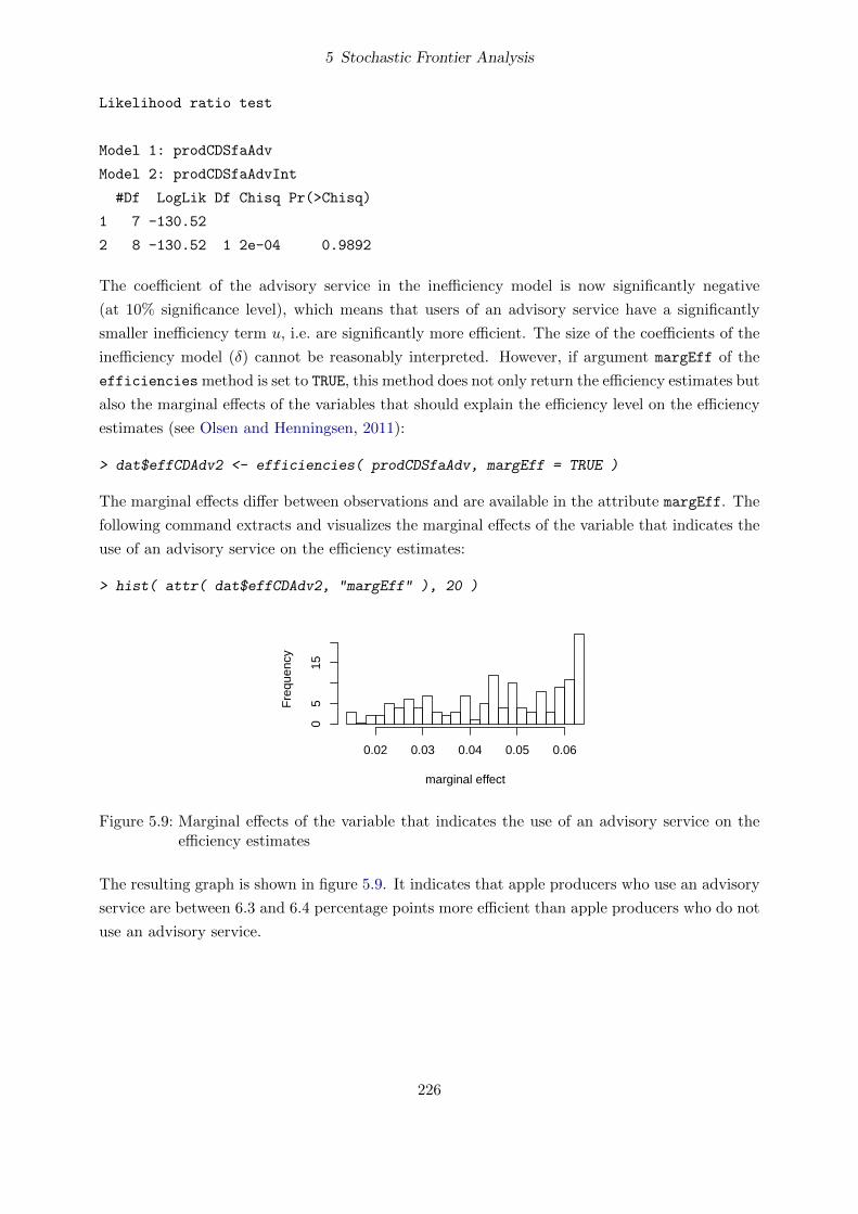
5 Stochastic Frontier Analysis
Likelihood ratio test
Model 1: prodCDSfaAdv
Model 2: prodCDSfaAdvInt
#Df LogLik Df Chisq Pr(>Chisq)
1 7 -130.52
2 8 -130.52 1 2e-04 0.9892
The coefficient of the advisory service in the inefficiency model is now significantly negative
(at 10% significance level), which means that users of an advisory service have a significantly
smaller inefficiency term u, i.e. are significantly more efficient. The size of the coefficients of the
inefficiency model (δ) cannot be reasonably interpreted. However, if argument margEff of the
efficiencies method is set to TRUE, this method does not only return the efficiency estimates but
also the marginal effects of the variables that should explain the efficiency level on the efficiency
estimates (see Olsen and Henningsen, 2011):
> dat$effCDAdv2 <- efficiencies( prodCDSfaAdv, margEff = TRUE )
The marginal effects differ between observations and are available in the attribute margEff. The
following command extracts and visualizes the marginal effects of the variable that indicates the
use of an advisory service on the efficiency estimates:
> hist( attr( dat$effCDAdv2, "margEff" ), 20 )
marginal effect
Fre
quen
cy
0.02 0.03 0.04 0.05 0.06
05
15
Figure 5.9: Marginal effects of the variable that indicates the use of an advisory service on theefficiency estimates
The resulting graph is shown in figure 5.9. It indicates that apple producers who use an advisory
service are between 6.3 and 6.4 percentage points more efficient than apple producers who do not
use an advisory service.
226
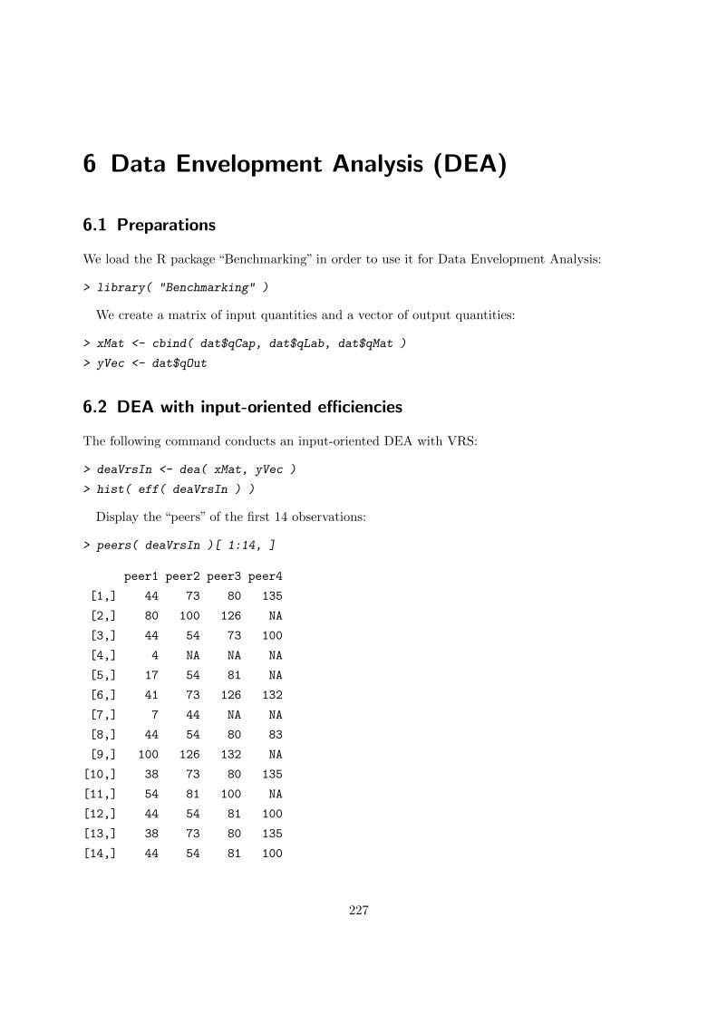
6 Data Envelopment Analysis (DEA)
6.1 Preparations
We load the R package “Benchmarking” in order to use it for Data Envelopment Analysis:
> library( "Benchmarking" )
We create a matrix of input quantities and a vector of output quantities:
> xMat <- cbind( dat$qCap, dat$qLab, dat$qMat )
> yVec <- dat$qOut
6.2 DEA with input-oriented efficiencies
The following command conducts an input-oriented DEA with VRS:
> deaVrsIn <- dea( xMat, yVec )
> hist( eff( deaVrsIn ) )
Display the “peers” of the first 14 observations:
> peers( deaVrsIn )[ 1:14, ]
peer1 peer2 peer3 peer4
[1,] 44 73 80 135
[2,] 80 100 126 NA
[3,] 44 54 73 100
[4,] 4 NA NA NA
[5,] 17 54 81 NA
[6,] 41 73 126 132
[7,] 7 44 NA NA
[8,] 44 54 80 83
[9,] 100 126 132 NA
[10,] 38 73 80 135
[11,] 54 81 100 NA
[12,] 44 54 81 100
[13,] 38 73 80 135
[14,] 44 54 81 100
227

6 Data Envelopment Analysis (DEA)
Display the λs of the first 14 observations:
> lambda( deaVrsIn )[ 1:14, ]
L4 L7 L17 L19 L38 L41 L44 L54 L61 L64
[1,] 0 0 0.00000000 0 0.00000000 0.0000000 8.707089e-02 0.00000000 0 0
[2,] 0 0 0.00000000 0 0.00000000 0.0000000 0.000000e+00 0.00000000 0 0
[3,] 0 0 0.00000000 0 0.00000000 0.0000000 5.466873e-02 0.34157362 0 0
[4,] 1 0 0.00000000 0 0.00000000 0.0000000 0.000000e+00 0.00000000 0 0
[5,] 0 0 0.07874218 0 0.00000000 0.0000000 0.000000e+00 0.62716635 0 0
[6,] 0 0 0.00000000 0 0.00000000 0.9520817 0.000000e+00 0.00000000 0 0
[7,] 0 1 0.00000000 0 0.00000000 0.0000000 2.000151e-12 0.00000000 0 0
[8,] 0 0 0.00000000 0 0.00000000 0.0000000 3.922860e-01 0.34818591 0 0
[9,] 0 0 0.00000000 0 0.00000000 0.0000000 0.000000e+00 0.00000000 0 0
[10,] 0 0 0.00000000 0 0.06541405 0.0000000 0.000000e+00 0.00000000 0 0
[11,] 0 0 0.00000000 0 0.00000000 0.0000000 0.000000e+00 0.52820862 0 0
[12,] 0 0 0.00000000 0 0.00000000 0.0000000 4.407646e-01 0.09749327 0 0
[13,] 0 0 0.00000000 0 0.01725343 0.0000000 0.000000e+00 0.00000000 0 0
[14,] 0 0 0.00000000 0 0.00000000 0.0000000 3.593759e-01 0.44329381 0 0
L73 L74 L78 L80 L81 L83 L100 L103
[1,] 0.243735897 0 0 0.6423537 0.00000000 0.00000000 0.0000000 0
[2,] 0.000000000 0 0 0.5147430 0.00000000 0.00000000 0.3620871 0
[3,] 0.153372277 0 0 0.0000000 0.00000000 0.00000000 0.4503854 0
[4,] 0.000000000 0 0 0.0000000 0.00000000 0.00000000 0.0000000 0
[5,] 0.000000000 0 0 0.0000000 0.29409147 0.00000000 0.0000000 0
[6,] 0.002769034 0 0 0.0000000 0.00000000 0.00000000 0.0000000 0
[7,] 0.000000000 0 0 0.0000000 0.00000000 0.00000000 0.0000000 0
[8,] 0.000000000 0 0 0.2101886 0.00000000 0.04933947 0.0000000 0
[9,] 0.000000000 0 0 0.0000000 0.00000000 0.00000000 0.6917918 0
[10,] 0.068686498 0 0 0.2825911 0.00000000 0.00000000 0.0000000 0
[11,] 0.000000000 0 0 0.0000000 0.25455055 0.00000000 0.2172408 0
[12,] 0.000000000 0 0 0.0000000 0.29388540 0.00000000 0.1678567 0
[13,] 0.383969646 0 0 0.5669254 0.00000000 0.00000000 0.0000000 0
[14,] 0.000000000 0 0 0.0000000 0.04033289 0.00000000 0.1569974 0
L126 L129 L132 L135 L137
[1,] 0.000000000 0 0.00000000 0.02683954 0
[2,] 0.123169836 0 0.00000000 0.00000000 0
[3,] 0.000000000 0 0.00000000 0.00000000 0
[4,] 0.000000000 0 0.00000000 0.00000000 0
[5,] 0.000000000 0 0.00000000 0.00000000 0
[6,] 0.008468157 0 0.03668108 0.00000000 0
228

6 Data Envelopment Analysis (DEA)
[7,] 0.000000000 0 0.00000000 0.00000000 0
[8,] 0.000000000 0 0.00000000 0.00000000 0
[9,] 0.249102366 0 0.05910586 0.00000000 0
[10,] 0.000000000 0 0.00000000 0.58330837 0
[11,] 0.000000000 0 0.00000000 0.00000000 0
[12,] 0.000000000 0 0.00000000 0.00000000 0
[13,] 0.000000000 0 0.00000000 0.03185153 0
[14,] 0.000000000 0 0.00000000 0.00000000 0
The following commands display the “slack” of the first 14 observations in an input-oriented
DEA with VRS:
> deaVrsIn <- dea( xMat, yVec, SLACK = TRUE )
> sum( deaVrsIn$slack )
[1] 62
> deaVrsIn$sx[ 1:14, ]
sx1 sx2 sx3
[1,] 0 0 0.00000
[2,] 0 0 345.70719
[3,] 0 0 0.00000
[4,] 0 0 0.00000
[5,] 0 0 38.54949
[6,] 0 0 0.00000
[7,] 0 0 0.00000
[8,] 0 0 0.00000
[9,] 0 0 1624.33417
[10,] 0 0 0.00000
[11,] 0 0 12993.07250
[12,] 0 0 0.00000
[13,] 0 0 0.00000
[14,] 0 0 0.00000
> deaVrsIn$sy[ 1:14, ]
[1] 0 0 0 0 0 0 0 0 0 0 0 0 0 0
The following command conducts an input-oriented DEA with CRS:
> deaCrsIn <- dea( xMat, yVec, RTS = "crs" )
> hist( eff( deaCrsIn ) )
229

6 Data Envelopment Analysis (DEA)
We can calculate the scale efficiencies by:
> se <- eff( deaCrsIn ) / eff( deaVrsIn )
> hist( se )
The following command conducts an input-oriented DEA with DRS
> deaDrsIn <- dea( xMat, yVec, RTS = "drs" )
> hist( eff( deaDrsIn ) )
And we check if firms are too small or too large. This is the number of observations that
produce at the scale below the optimal scale size:
> sum( eff( deaVrsIn ) - eff( deaDrsIn ) > 1e-4 )
[1] 117
6.3 DEA with output-oriented efficiencies
The following command conducts an output-oriented DEA with VRS:
> deaVrsOut <- dea( xMat, yVec, ORIENTATION = "out" )
> hist( efficiencies( deaVrsOut ) )
The following command conducts an output-oriented DEA with CRS:
> deaCrsOut <- dea( xMat, yVec, RTS = "crs", ORIENTATION = "out" )
> hist( eff( deaCrsOut ) )
In case of CRS, input-oriented efficiencies are equivalent to output-oriented efficiencies:
> all.equal( eff( deaCrsIn ), 1 / eff( deaCrsOut ) )
[1] TRUE
6.4 DEA with “super efficiencies”
The following command obtains “super efficiencies” for an input-oriented DEA with CRS:
> sdeaVrsIn <- sdea( xMat, yVec )
> hist( eff( sdeaVrsIn ) )
6.5 DEA with graph hyperbolic efficiencies
The following command conducts a DEA with graph hyperbolic efficiencies and VRS:
> deaVrsGraph <- dea( xMat, yVec, ORIENTATION = "graph" )
> hist( eff( deaVrsGraph ) )
> plot( eff( deaVrsIn ), eff( deaVrsGraph ) )
> abline(0,1)
230

7 Panel Data and Technological Change
Until now, we have only analyzed cross-sectional data, i.e. all observations refer to the same period
of time. Hence, it was reasonable to assume that the same technology is available to all firms
(observations). However, when analyzing time series data or panel data, i.e. when observations
can originate from different time periods, different technologies might be available in the different
time periods due to technological change. Hence, the state of the available technologies must be
included as an explanatory variable in order to conduct a reasonable production analysis. Often,
a time trend is used as a proxy for a gradually changing state of the available technologies.
We will demonstrate how to analyze production technologies with data from different time
periods by using a balanced panel data set of annual data collected from 43 smallholder rice
producers in the Tarlac region of the Philippines between 1990 and 1997. We loaded this data set
(riceProdPhil) in section 1.3.2. As it does not contain information about the panel structure,
we created a copy of the data set (pdat) that includes information on the panel structure.
7.1 Average Production Functions with Technological Change
In case of an applied production analysis with time-series data or panel data, usually the time (t)
is included as additional explanatory variable in the production function:
y = f(x, t). (7.1)
This function can be used to analyze how the time (t) affects the (available) production technol-
ogy.
The average production technology (potentially depending on the time period) can be estimated
from panel data sets by the OLS method (i.e. “pooled”) or by any of the usual panel data methods
(e.g. fixed effects, random effects).
7.1.1 Cobb-Douglas Production Function with Technological Change
In case of a Cobb-Douglas production function, usually a linear time trend is added to account
for technological change:
ln y = α0 +∑i
αi ln xi + αt t (7.2)
231

7 Panel Data and Technological Change
Given this specification, the coefficient of the (linear) time trend can be interpreted as the rate
of technological change per unit of the time variable t:
αt = ∂ ln y∂t
= ∂ ln y∂y
∂y
∂t≈
∆yy
∆x (7.3)
7.1.1.1 Pooled estimation of the Cobb-Douglas Production Function with Technological
Change
The pooled estimation can be done by:
> riceCdTime <- lm( log( PROD ) ~ log( AREA ) + log( LABOR ) + log( NPK ) +
+ mYear, data = riceProdPhil )
> summary( riceCdTime )
Call:
lm(formula = log(PROD) ~ log(AREA) + log(LABOR) + log(NPK) +
mYear, data = riceProdPhil)
Residuals:
Min 1Q Median 3Q Max
-1.83351 -0.16006 0.05329 0.22110 0.86745
Coefficients:
Estimate Std. Error t value Pr(>|t|)
(Intercept) -1.665096 0.248509 -6.700 8.68e-11 ***
log(AREA) 0.333214 0.062403 5.340 1.71e-07 ***
log(LABOR) 0.395573 0.066421 5.956 6.48e-09 ***
log(NPK) 0.270847 0.041027 6.602 1.57e-10 ***
mYear 0.010090 0.008007 1.260 0.208
---
Signif. codes: 0 ‘***’ 0.001 ‘**’ 0.01 ‘*’ 0.05 ‘.’ 0.1 ‘ ’ 1
Residual standard error: 0.3299 on 339 degrees of freedom
Multiple R-squared: 0.86, Adjusted R-squared: 0.8583
F-statistic: 520.6 on 4 and 339 DF, p-value: < 2.2e-16
The estimation result indicates an annual rate of technical change of 1%, but this is not statisti-
cally different from 0%, which means no technological change.
The command above can be simplified by using the pre-calculated logarithmic (and mean-
scaled) quantities:
232

7 Panel Data and Technological Change
> riceCdTimeS <- lm( lProd ~ lArea + lLabor + lNpk + mYear, data = riceProdPhil )
> summary( riceCdTimeS )
Call:
lm(formula = lProd ~ lArea + lLabor + lNpk + mYear, data = riceProdPhil)
Residuals:
Min 1Q Median 3Q Max
-1.83351 -0.16006 0.05329 0.22110 0.86745
Coefficients:
Estimate Std. Error t value Pr(>|t|)
(Intercept) -0.015590 0.019325 -0.807 0.420
lArea 0.333214 0.062403 5.340 1.71e-07 ***
lLabor 0.395573 0.066421 5.956 6.48e-09 ***
lNpk 0.270847 0.041027 6.602 1.57e-10 ***
mYear 0.010090 0.008007 1.260 0.208
---
Signif. codes: 0 ‘***’ 0.001 ‘**’ 0.01 ‘*’ 0.05 ‘.’ 0.1 ‘ ’ 1
Residual standard error: 0.3299 on 339 degrees of freedom
Multiple R-squared: 0.86, Adjusted R-squared: 0.8583
F-statistic: 520.6 on 4 and 339 DF, p-value: < 2.2e-16
The intercept has changed because of the mean-scaling of the input and output quantities but
all slope parameters are unaffected by using the pre-calculated logarithmic (and mean-scaled)
quantities:
> all.equal( coef( riceCdTime )[-1], coef( riceCdTimeS )[-1],
+ check.attributes = FALSE )
[1] TRUE
7.1.1.2 Panel data estimations of the Cobb-Douglas Production Function with
Technological Change
The panel data estimation with fixed individual effects can be done by:
> riceCdTimeFe <- plm( lProd ~ lArea + lLabor + lNpk + mYear, data = pdat )
> summary( riceCdTimeFe )
Oneway (individual) effect Within Model
233

7 Panel Data and Technological Change
Call:
plm(formula = lProd ~ lArea + lLabor + lNpk + mYear, data = pdat)
Balanced Panel: n=43, T=8, N=344
Residuals :
Min. 1st Qu. Median 3rd Qu. Max.
-1.5900 -0.1570 0.0456 0.1780 0.8180
Coefficients :
Estimate Std. Error t-value Pr(>|t|)
lArea 0.5607756 0.0785370 7.1403 7.195e-12 ***
lLabor 0.2549108 0.0690631 3.6910 0.0002657 ***
lNpk 0.1748528 0.0484684 3.6076 0.0003625 ***
mYear 0.0130908 0.0071824 1.8226 0.0693667 .
---
Signif. codes: 0 ‘***’ 0.001 ‘**’ 0.01 ‘*’ 0.05 ‘.’ 0.1 ‘ ’ 1
Total Sum of Squares: 43.632
Residual Sum of Squares: 24.872
R-Squared : 0.42995
Adj. R-Squared : 0.3712
F-statistic: 56.0008 on 4 and 297 DF, p-value: < 2.22e-16
And the panel data estimation with random individual effects can be done by:
> riceCdTimeRan <- plm( lProd ~ lArea + lLabor + lNpk + mYear, data = pdat,
+ model = "random" )
> summary( riceCdTimeRan )
Oneway (individual) effect Random Effect Model
(Swamy-Arora's transformation)
Call:
plm(formula = lProd ~ lArea + lLabor + lNpk + mYear, data = pdat,
model = "random")
Balanced Panel: n=43, T=8, N=344
Effects:
var std.dev share
234

7 Panel Data and Technological Change
idiosyncratic 0.08375 0.28939 0.8
individual 0.02088 0.14451 0.2
theta: 0.4222
Residuals :
Min. 1st Qu. Median 3rd Qu. Max.
-1.7500 -0.1430 0.0485 0.1910 0.8520
Coefficients :
Estimate Std. Error t-value Pr(>|t|)
(Intercept) -0.0213044 0.0292268 -0.7289 0.4665
lArea 0.4563002 0.0662979 6.8826 2.854e-11 ***
lLabor 0.3190041 0.0647524 4.9265 1.311e-06 ***
lNpk 0.2268399 0.0426651 5.3168 1.921e-07 ***
mYear 0.0115453 0.0071921 1.6053 0.1094
---
Signif. codes: 0 ‘***’ 0.001 ‘**’ 0.01 ‘*’ 0.05 ‘.’ 0.1 ‘ ’ 1
Total Sum of Squares: 117.05
Residual Sum of Squares: 29.195
R-Squared : 0.75058
Adj. R-Squared : 0.73968
F-statistic: 255.045 on 4 and 339 DF, p-value: < 2.22e-16
A variable-coefficient model for panel model with individual-specific coefficients can be esti-
mated by:
> riceCdTimeVc <- pvcm( lProd ~ lArea + lLabor + lNpk + mYear, data = pdat )
> summary( riceCdTimeVc )
Oneway (individual) effect No-pooling model
Call:
pvcm(formula = lProd ~ lArea + lLabor + lNpk + mYear, data = pdat)
Balanced Panel: n=43, T=8, N=344
Residuals:
Min. 1st Qu. Median Mean 3rd Qu. Max.
-0.817500 -0.081970 0.006677 0.000000 0.093980 0.554100
235

7 Panel Data and Technological Change
Coefficients:
(Intercept) lArea lLabor lNpk
Min. :-3.8110 Min. :-5.2850 Min. :-2.72761 Min. :-1.3094
1st Qu.:-0.3006 1st Qu.:-0.4200 1st Qu.:-0.30989 1st Qu.:-0.1867
Median : 0.1145 Median : 0.6978 Median : 0.08778 Median : 0.1050
Mean : 0.1839 Mean : 0.5896 Mean : 0.06079 Mean : 0.1265
3rd Qu.: 0.5617 3rd Qu.: 1.8914 3rd Qu.: 0.61479 3rd Qu.: 0.3808
Max. : 3.7270 Max. : 4.7633 Max. : 1.75595 Max. : 1.7180
NA's :18
mYear
Min. :-0.471049
1st Qu.:-0.044359
Median :-0.008111
Mean :-0.012327
3rd Qu.: 0.054743
Max. : 0.275875
Total Sum of Squares: 2861.8
Residual Sum of Squares: 8.9734
Multiple R-Squared: 0.99686
A pooled estimation can also be done by
> riceCdTimePool <- plm( lProd ~ lArea + lLabor + lNpk + mYear, data = pdat,
+ model = "pooling" )
This gives the same estimated coefficients as the model estimated by lm:
> all.equal( coef( riceCdTimeS ), coef( riceCdTimePool ) )
[1] TRUE
A Hausman test can be used to check the consistency of the random-effects estimator:
> phtest( riceCdTimeRan, riceCdTimeFe )
Hausman Test
data: lProd ~ lArea + lLabor + lNpk + mYear
chisq = 14.6204, df = 4, p-value = 0.005557
alternative hypothesis: one model is inconsistent
236

7 Panel Data and Technological Change
The Hausman test clearly shows that the random-effects estimator is inconsistent (due to corre-
lation between the individual effects and the explanatory variables).
Now, we test the poolability of the model:
> pooltest( riceCdTimePool, riceCdTimeFe )
F statistic
data: lProd ~ lArea + lLabor + lNpk + mYear
F = 3.4175, df1 = 42, df2 = 297, p-value = 4.038e-10
alternative hypothesis: unstability
> pooltest( riceCdTimePool, riceCdTimeVc )
F statistic
data: lProd ~ lArea + lLabor + lNpk + mYear
F = 1.9113, df1 = 210, df2 = 129, p-value = 4.022e-05
alternative hypothesis: unstability
> pooltest( riceCdTimeFe, riceCdTimeVc )
F statistic
data: lProd ~ lArea + lLabor + lNpk + mYear
F = 1.3605, df1 = 168, df2 = 129, p-value = 0.03339
alternative hypothesis: unstability
The pooled model (riceCdTimePool) is clearly rejected in favour of the model with fixed indi-
vidual effects (riceCdTimeFe) and the variable-coefficient model (riceCdTimeVc). The model
with fixed individual effects (riceCdTimeFe) is rejected in favor of the variable-coefficient model
(riceCdTimeVc) at 5% significance level but not at 1% significance level.
7.1.2 Translog Production Function with Constant and Neutral Technological
Change
A Translog production function that accounts for constant and neutral (unbiased) technological
change has following specification:
ln y = α0 +∑i
αi ln xi + 12∑i
∑j
αij ln xi ln xj + αt t (7.4)
In this specification, the rate of technological change is
∂ ln y∂t
= αt (7.5)
237

7 Panel Data and Technological Change
and the output elasticities are the same as in the time-invariant Translog production func-
tion (2.105):
εi = ∂ ln y∂ ln xi
= αi +∑j
αij ln xj (7.6)
In order to be able to interpret the first-order coefficients of the (logarithmic) input quantities
(αi) as output elasticities (εi) at the sample mean, we use the mean-scaled input quantities. We
also use the mean-scaled output quantity in order to use the same variables as Coelli et al. (2005,
p. 250).
7.1.2.1 Pooled estimation of the Translog Production Function with Constant and Neutral
Technological Change
The following command estimates a Translog production function that can account for constant
and neutral technical change:
> riceTlTime <- lm( lProd ~ lArea + lLabor + lNpk +
+ I( 0.5 * lArea^2 ) + I( 0.5 * lLabor^2 ) + I( 0.5 * lNpk^2 ) +
+ I( lArea * lLabor ) + I( lArea * lNpk ) + I( lLabor * lNpk ) + mYear,
+ data = riceProdPhil )
> summary( riceTlTime )
Call:
lm(formula = lProd ~ lArea + lLabor + lNpk + I(0.5 * lArea^2) +
I(0.5 * lLabor^2) + I(0.5 * lNpk^2) + I(lArea * lLabor) +
I(lArea * lNpk) + I(lLabor * lNpk) + mYear, data = riceProdPhil)
Residuals:
Min 1Q Median 3Q Max
-1.52184 -0.18121 0.04356 0.22298 0.87019
Coefficients:
Estimate Std. Error t value Pr(>|t|)
(Intercept) 0.013756 0.024645 0.558 0.57712
lArea 0.588097 0.085162 6.906 2.54e-11 ***
lLabor 0.191764 0.080876 2.371 0.01831 *
lNpk 0.197875 0.051605 3.834 0.00015 ***
I(0.5 * lArea^2) -0.435547 0.247491 -1.760 0.07935 .
I(0.5 * lLabor^2) -0.742242 0.303236 -2.448 0.01489 *
I(0.5 * lNpk^2) 0.020367 0.097907 0.208 0.83534
I(lArea * lLabor) 0.678647 0.216594 3.133 0.00188 **
238

7 Panel Data and Technological Change
I(lArea * lNpk) 0.063920 0.145613 0.439 0.66097
I(lLabor * lNpk) -0.178286 0.138611 -1.286 0.19926
mYear 0.012682 0.007795 1.627 0.10468
---
Signif. codes: 0 ‘***’ 0.001 ‘**’ 0.01 ‘*’ 0.05 ‘.’ 0.1 ‘ ’ 1
Residual standard error: 0.3184 on 333 degrees of freedom
Multiple R-squared: 0.8719, Adjusted R-squared: 0.868
F-statistic: 226.6 on 10 and 333 DF, p-value: < 2.2e-16
In the Translog production function that accounts for constant and neutral technological change,
the monotonicity conditions are fulfilled at the sample mean and the estimated output elasticities
of land, labor and fertilizer are 0.588, 0.192, and 0.198, respectively, at the sample mean. The
estimated (constant) annual rate of technological progress is around 1.3%.
Conduct a Wald test to test whether the Translog production function outperforms the Cobb-
Douglas production function:
> library( "lmtest" )
> waldtest( riceCdTimeS, riceTlTime )
Wald test
Model 1: lProd ~ lArea + lLabor + lNpk + mYear
Model 2: lProd ~ lArea + lLabor + lNpk + I(0.5 * lArea^2) + I(0.5 * lLabor^2) +
I(0.5 * lNpk^2) + I(lArea * lLabor) + I(lArea * lNpk) + I(lLabor *
lNpk) + mYear
Res.Df Df F Pr(>F)
1 339
2 333 6 5.1483 4.451e-05 ***
---
Signif. codes: 0 ‘***’ 0.001 ‘**’ 0.01 ‘*’ 0.05 ‘.’ 0.1 ‘ ’ 1
The Cobb-Douglas specification is clearly rejected in favour of the Translog specification for the
pooled estimation.
7.1.2.2 Panel-data estimations of the Translog Production Function with Constant and
Neutral Technological Change
The following command estimates a Translog production function that can account for constant
and neutral technical change with fixed individual effects:
> riceTlTimeFe <- plm( lProd ~ lArea + lLabor + lNpk +
+ I( 0.5 * lArea^2 ) + I( 0.5 * lLabor^2 ) + I( 0.5 * lNpk^2 ) +
239

7 Panel Data and Technological Change
+ I( lArea * lLabor ) + I( lArea * lNpk ) + I( lLabor * lNpk ) + mYear,
+ data = pdat, model = "within" )
> summary( riceTlTimeFe )
Oneway (individual) effect Within Model
Call:
plm(formula = lProd ~ lArea + lLabor + lNpk + I(0.5 * lArea^2) +
I(0.5 * lLabor^2) + I(0.5 * lNpk^2) + I(lArea * lLabor) +
I(lArea * lNpk) + I(lLabor * lNpk) + mYear, data = pdat,
model = "within")
Balanced Panel: n=43, T=8, N=344
Residuals :
Min. 1st Qu. Median 3rd Qu. Max.
-1.0100 -0.1450 0.0191 0.1680 0.7460
Coefficients :
Estimate Std. Error t-value Pr(>|t|)
lArea 0.5828102 0.1173298 4.9673 1.16e-06 ***
lLabor 0.0473355 0.0848594 0.5578 0.577402
lNpk 0.1211928 0.0610114 1.9864 0.047927 *
I(0.5 * lArea^2) -0.8543901 0.2861292 -2.9860 0.003067 **
I(0.5 * lLabor^2) -0.6217163 0.2935429 -2.1180 0.035025 *
I(0.5 * lNpk^2) 0.0429446 0.0987119 0.4350 0.663849
I(lArea * lLabor) 0.5867063 0.2125686 2.7601 0.006145 **
I(lArea * lNpk) 0.1167509 0.1461380 0.7989 0.424995
I(lLabor * lNpk) -0.2371219 0.1268671 -1.8691 0.062619 .
mYear 0.0165309 0.0069206 2.3887 0.017547 *
---
Signif. codes: 0 ‘***’ 0.001 ‘**’ 0.01 ‘*’ 0.05 ‘.’ 0.1 ‘ ’ 1
Total Sum of Squares: 43.632
Residual Sum of Squares: 21.912
R-Squared : 0.49781
Adj. R-Squared : 0.42111
F-statistic: 28.8456 on 10 and 291 DF, p-value: < 2.22e-16
And the panel data estimation with random individual effects can be done by:
240

7 Panel Data and Technological Change
> riceTlTimeRan <- plm( lProd ~ lArea + lLabor + lNpk +
+ I( 0.5 * lArea^2 ) + I( 0.5 * lLabor^2 ) + I( 0.5 * lNpk^2 ) +
+ I( lArea * lLabor ) + I( lArea * lNpk ) + I( lLabor * lNpk ) + mYear,
+ data = pdat, model = "random" )
> summary( riceTlTimeRan )
Oneway (individual) effect Random Effect Model
(Swamy-Arora's transformation)
Call:
plm(formula = lProd ~ lArea + lLabor + lNpk + I(0.5 * lArea^2) +
I(0.5 * lLabor^2) + I(0.5 * lNpk^2) + I(lArea * lLabor) +
I(lArea * lNpk) + I(lLabor * lNpk) + mYear, data = pdat,
model = "random")
Balanced Panel: n=43, T=8, N=344
Effects:
var std.dev share
idiosyncratic 0.07530 0.27440 0.79
individual 0.01997 0.14130 0.21
theta: 0.434
Residuals :
Min. 1st Qu. Median 3rd Qu. Max.
-1.3900 -0.1620 0.0456 0.1840 0.7980
Coefficients :
Estimate Std. Error t-value Pr(>|t|)
(Intercept) 0.0213211 0.0347371 0.6138 0.539776
lArea 0.6831045 0.0922069 7.4084 1.061e-12 ***
lLabor 0.0974523 0.0804060 1.2120 0.226370
lNpk 0.1708366 0.0546853 3.1240 0.001941 **
I(0.5 * lArea^2) -0.4275328 0.2468086 -1.7322 0.084156 .
I(0.5 * lLabor^2) -0.6367899 0.2872825 -2.2166 0.027326 *
I(0.5 * lNpk^2) 0.0307547 0.0957745 0.3211 0.748324
I(lArea * lLabor) 0.5666863 0.2059076 2.7521 0.006245 **
I(lArea * lNpk) 0.1037657 0.1421739 0.7299 0.465995
I(lLabor * lNpk) -0.2055786 0.1277476 -1.6093 0.108508
mYear 0.0142202 0.0070184 2.0261 0.043549 *
241

7 Panel Data and Technological Change
---
Signif. codes: 0 ‘***’ 0.001 ‘**’ 0.01 ‘*’ 0.05 ‘.’ 0.1 ‘ ’ 1
Total Sum of Squares: 114.08
Residual Sum of Squares: 26.624
R-Squared : 0.76662
Adj. R-Squared : 0.74211
F-statistic: 109.386 on 10 and 333 DF, p-value: < 2.22e-16
The Translog production function cannot be estimated by a variable-coefficient model for panel
model with our data set, because the number of time periods in the data set is smaller than the
number of the coefficients.
A pooled estimation can be done by
> riceTlTimePool <- plm( lProd ~ lArea + lLabor + lNpk +
+ I( 0.5 * lArea^2 ) + I( 0.5 * lLabor^2 ) + I( 0.5 * lNpk^2 ) +
+ I( lArea * lLabor ) + I( lArea * lNpk ) + I( lLabor * lNpk ) + mYear,
+ data = pdat, model = "pooling" )
> summary(riceTlTimePool)
Oneway (individual) effect Pooling Model
Call:
plm(formula = lProd ~ lArea + lLabor + lNpk + I(0.5 * lArea^2) +
I(0.5 * lLabor^2) + I(0.5 * lNpk^2) + I(lArea * lLabor) +
I(lArea * lNpk) + I(lLabor * lNpk) + mYear, data = pdat,
model = "pooling")
Balanced Panel: n=43, T=8, N=344
Residuals :
Min. 1st Qu. Median 3rd Qu. Max.
-1.5200 -0.1810 0.0436 0.2230 0.8700
Coefficients :
Estimate Std. Error t-value Pr(>|t|)
(Intercept) 0.0137557 0.0246454 0.5581 0.5771201
lArea 0.5880972 0.0851622 6.9056 2.542e-11 ***
lLabor 0.1917638 0.0808764 2.3711 0.0183052 *
lNpk 0.1978747 0.0516045 3.8344 0.0001505 ***
I(0.5 * lArea^2) -0.4355466 0.2474913 -1.7598 0.0793520 .
242

7 Panel Data and Technological Change
I(0.5 * lLabor^2) -0.7422415 0.3032362 -2.4477 0.0148916 *
I(0.5 * lNpk^2) 0.0203673 0.0979072 0.2080 0.8353358
I(lArea * lLabor) 0.6786472 0.2165937 3.1333 0.0018822 **
I(lArea * lNpk) 0.0639200 0.1456135 0.4390 0.6609677
I(lLabor * lNpk) -0.1782859 0.1386111 -1.2862 0.1992559
mYear 0.0126820 0.0077947 1.6270 0.1046801
---
Signif. codes: 0 ‘***’ 0.001 ‘**’ 0.01 ‘*’ 0.05 ‘.’ 0.1 ‘ ’ 1
Total Sum of Squares: 263.52
Residual Sum of Squares: 33.761
R-Squared : 0.87189
Adj. R-Squared : 0.84401
F-statistic: 226.623 on 10 and 333 DF, p-value: < 2.22e-16
This gives the same estimated coefficients as the model estimated by lm:
> all.equal( coef( riceTlTime ), coef( riceTlTimePool ) )
[1] TRUE
A Hausman test can be used to check the consistency of the random-effects estimator:
> phtest( riceTlTimeRan, riceTlTimeFe )
Hausman Test
data: lProd ~ lArea + lLabor + lNpk + I(0.5 * lArea^2) + I(0.5 * lLabor^2) + ...
chisq = 66.071, df = 10, p-value = 2.528e-10
alternative hypothesis: one model is inconsistent
The Hausman test clearly rejects the consistency of the random-effects estimator.
The following command tests the poolability of the model:
> pooltest( riceTlTimePool, riceTlTimeFe )
F statistic
data: lProd ~ lArea + lLabor + lNpk + I(0.5 * lArea^2) + I(0.5 * lLabor^2) + ...
F = 3.7469, df1 = 42, df2 = 291, p-value = 1.525e-11
alternative hypothesis: unstability
243

7 Panel Data and Technological Change
The pooled model (riceCdTimePool) is clearly rejected in favour of the model with fixed indi-
vidual effects (riceCdTimeFe), i.e. the individual effects are statistically significant.
The following commands test if the fit of Translog specification is significantly better than the
fit of the Cobb-Douglas specification:
> waldtest( riceCdTimeFe, riceTlTimeFe )
Wald test
Model 1: lProd ~ lArea + lLabor + lNpk + mYear
Model 2: lProd ~ lArea + lLabor + lNpk + I(0.5 * lArea^2) + I(0.5 * lLabor^2) +
I(0.5 * lNpk^2) + I(lArea * lLabor) + I(lArea * lNpk) + I(lLabor *
lNpk) + mYear
Res.Df Df Chisq Pr(>Chisq)
1 297
2 291 6 39.321 6.191e-07 ***
---
Signif. codes: 0 ‘***’ 0.001 ‘**’ 0.01 ‘*’ 0.05 ‘.’ 0.1 ‘ ’ 1
> waldtest( riceCdTimeRan, riceTlTimeRan )
Wald test
Model 1: lProd ~ lArea + lLabor + lNpk + mYear
Model 2: lProd ~ lArea + lLabor + lNpk + I(0.5 * lArea^2) + I(0.5 * lLabor^2) +
I(0.5 * lNpk^2) + I(lArea * lLabor) + I(lArea * lNpk) + I(lLabor *
lNpk) + mYear
Res.Df Df Chisq Pr(>Chisq)
1 339
2 333 6 30.077 3.8e-05 ***
---
Signif. codes: 0 ‘***’ 0.001 ‘**’ 0.01 ‘*’ 0.05 ‘.’ 0.1 ‘ ’ 1
> waldtest( riceCdTimePool, riceTlTimePool )
Wald test
Model 1: lProd ~ lArea + lLabor + lNpk + mYear
Model 2: lProd ~ lArea + lLabor + lNpk + I(0.5 * lArea^2) + I(0.5 * lLabor^2) +
I(0.5 * lNpk^2) + I(lArea * lLabor) + I(lArea * lNpk) + I(lLabor *
lNpk) + mYear
Res.Df Df Chisq Pr(>Chisq)
244

7 Panel Data and Technological Change
1 339
2 333 6 30.89 2.66e-05 ***
---
Signif. codes: 0 ‘***’ 0.001 ‘**’ 0.01 ‘*’ 0.05 ‘.’ 0.1 ‘ ’ 1
The Cobb-Douglas functional form is rejected in favour of the Translog functional for for all three
panel-specifications that we estimated above. The Wald test for the pooled model differs from
the Wald test that we did in section 7.1.2.1, because waldtest by default uses a finite sample
F statistic for models estimated by lm but uses a large sample Chi-squared statistic for models
estimated by plm. The test statistic used by waldtest can be specified by argument test.
7.1.3 Translog Production Function with Non-Constant and Non-Neutral
Technological Change
Technological change is not always constant and is not always neutral (unbiased). Therefore,
it might be more suitable to estimate a production function that can account for increasing or
decreasing rates of technological change as well as biased (e.g. labor saving) technological change.
This can be done by including a quadratic time trend and interaction terms between time and
input quantities:
ln y = α0 +∑i
αi ln xi + 12∑i
∑j
αij ln xi ln xj + αt t+∑i
αti ln xi + 12αtt t
2 (7.7)
In this specification, the rate of technological change depends on the input quantities and the
time period:
∂ ln y∂t
= αt +∑i
αti ln xi + αtt t (7.8)
and the output elasticities might change over time:
εi = ∂ ln y∂ ln xi
= αi +∑j
αij ln xj + αti t. (7.9)
7.1.3.1 Pooled Estimation of a Translog Production Function with Non-Constant and
Non-Neutral Technological Change
The following command estimates a Translog production function that can account for non-
constant rates of technological change as well as biased technological change:
> riceTlTimeNn <- lm( lProd ~ lArea + lLabor + lNpk +
+ I( 0.5 * lArea^2 ) + I( 0.5 * lLabor^2 ) + I( 0.5 * lNpk^2 ) +
+ I( lArea * lLabor ) + I( lArea * lNpk ) + I( lLabor * lNpk ) +
+ mYear + I( mYear * lArea ) + I( mYear * lLabor ) + I( mYear * lNpk ) +
245
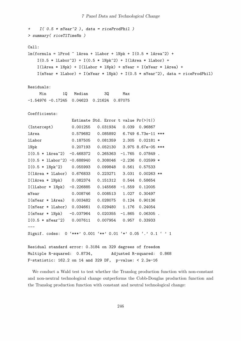
7 Panel Data and Technological Change
+ I( 0.5 * mYear^2 ), data = riceProdPhil )
> summary( riceTlTimeNn )
Call:
lm(formula = lProd ~ lArea + lLabor + lNpk + I(0.5 * lArea^2) +
I(0.5 * lLabor^2) + I(0.5 * lNpk^2) + I(lArea * lLabor) +
I(lArea * lNpk) + I(lLabor * lNpk) + mYear + I(mYear * lArea) +
I(mYear * lLabor) + I(mYear * lNpk) + I(0.5 * mYear^2), data = riceProdPhil)
Residuals:
Min 1Q Median 3Q Max
-1.54976 -0.17245 0.04623 0.21624 0.87075
Coefficients:
Estimate Std. Error t value Pr(>|t|)
(Intercept) 0.001255 0.031934 0.039 0.96867
lArea 0.579682 0.085892 6.749 6.73e-11 ***
lLabor 0.187505 0.081359 2.305 0.02181 *
lNpk 0.207193 0.052130 3.975 8.67e-05 ***
I(0.5 * lArea^2) -0.468372 0.265363 -1.765 0.07849 .
I(0.5 * lLabor^2) -0.688940 0.308046 -2.236 0.02599 *
I(0.5 * lNpk^2) 0.055993 0.099848 0.561 0.57533
I(lArea * lLabor) 0.676833 0.223271 3.031 0.00263 **
I(lArea * lNpk) 0.082374 0.151312 0.544 0.58654
I(lLabor * lNpk) -0.226885 0.145568 -1.559 0.12005
mYear 0.008746 0.008513 1.027 0.30497
I(mYear * lArea) 0.003482 0.028075 0.124 0.90136
I(mYear * lLabor) 0.034661 0.029480 1.176 0.24054
I(mYear * lNpk) -0.037964 0.020355 -1.865 0.06305 .
I(0.5 * mYear^2) 0.007611 0.007954 0.957 0.33933
---
Signif. codes: 0 ‘***’ 0.001 ‘**’ 0.01 ‘*’ 0.05 ‘.’ 0.1 ‘ ’ 1
Residual standard error: 0.3184 on 329 degrees of freedom
Multiple R-squared: 0.8734, Adjusted R-squared: 0.868
F-statistic: 162.2 on 14 and 329 DF, p-value: < 2.2e-16
We conduct a Wald test to test whether the Translog production function with non-constant
and non-neutral technological change outperforms the Cobb-Douglas production function and
the Translog production function with constant and neutral technological change:
246

7 Panel Data and Technological Change
> waldtest( riceCdTimeS, riceTlTimeNn )
Wald test
Model 1: lProd ~ lArea + lLabor + lNpk + mYear
Model 2: lProd ~ lArea + lLabor + lNpk + I(0.5 * lArea^2) + I(0.5 * lLabor^2) +
I(0.5 * lNpk^2) + I(lArea * lLabor) + I(lArea * lNpk) + I(lLabor *
lNpk) + mYear + I(mYear * lArea) + I(mYear * lLabor) + I(mYear *
lNpk) + I(0.5 * mYear^2)
Res.Df Df F Pr(>F)
1 339
2 329 10 3.488 0.00022 ***
---
Signif. codes: 0 ‘***’ 0.001 ‘**’ 0.01 ‘*’ 0.05 ‘.’ 0.1 ‘ ’ 1
> waldtest( riceTlTime, riceTlTimeNn )
Wald test
Model 1: lProd ~ lArea + lLabor + lNpk + I(0.5 * lArea^2) + I(0.5 * lLabor^2) +
I(0.5 * lNpk^2) + I(lArea * lLabor) + I(lArea * lNpk) + I(lLabor *
lNpk) + mYear
Model 2: lProd ~ lArea + lLabor + lNpk + I(0.5 * lArea^2) + I(0.5 * lLabor^2) +
I(0.5 * lNpk^2) + I(lArea * lLabor) + I(lArea * lNpk) + I(lLabor *
lNpk) + mYear + I(mYear * lArea) + I(mYear * lLabor) + I(mYear *
lNpk) + I(0.5 * mYear^2)
Res.Df Df F Pr(>F)
1 333
2 329 4 0.9976 0.4089
The fit of the Translog specification with non-constant and non-neutral technological change is
significantly better than the fit of the Cobb-Douglas specification but it is not significantly better
than the fit of the Translog specification with constant and neutral technological change.
In order to simplify the calculation of the output elasticities (with equation 7.9) and the
annual rates of technological change (with equation 7.8), we create shortcuts for the estimated
coefficients:
> a1 <- coef( riceTlTimeNn )[ "lArea" ]
> a2 <- coef( riceTlTimeNn )[ "lLabor" ]
> a3 <- coef( riceTlTimeNn )[ "lNpk" ]
> at <- coef( riceTlTimeNn )[ "mYear" ]
247

7 Panel Data and Technological Change
> a11 <- coef( riceTlTimeNn )[ "I(0.5 * lArea^2)" ]
> a22 <- coef( riceTlTimeNn )[ "I(0.5 * lLabor^2)" ]
> a33 <- coef( riceTlTimeNn )[ "I(0.5 * lNpk^2)" ]
> att <- coef( riceTlTimeNn )[ "I(0.5 * mYear^2)" ]
> a12 <- a21 <- coef( riceTlTimeNn )[ "I(lArea * lLabor)" ]
> a13 <- a31 <- coef( riceTlTimeNn )[ "I(lArea * lNpk)" ]
> a23 <- a32 <- coef( riceTlTimeNn )[ "I(lLabor * lNpk)" ]
> a1t <- at1 <- coef( riceTlTimeNn )[ "I(mYear * lArea)" ]
> a2t <- at2 <- coef( riceTlTimeNn )[ "I(mYear * lLabor)" ]
> a3t <- at3 <- coef( riceTlTimeNn )[ "I(mYear * lNpk)" ]
Now, we can use the following commands to calculate the partial output elasticities:
> riceProdPhil$eArea <- with( riceProdPhil,
+ a1 + a11 * lArea + a12 * lLabor + a13 * lNpk + a1t * mYear )
> riceProdPhil$eLabor <- with( riceProdPhil,
+ a2 + a21 * lArea + a22 * lLabor + a23 * lNpk + a2t * mYear )
> riceProdPhil$eNpk <- with( riceProdPhil,
+ a3 + a31 * lArea + a32 * lLabor + a33 * lNpk + a3t * mYear )
We can calculate the elasticity of scale by taken the sum over all partial output elasticities:
> riceProdPhil$eScale <- with( riceProdPhil, eArea + eLabor + eNpk )
We can visualize (the variation of) the output elasticities and the elasticity of scale with
histograms:
> hist( riceProdPhil$eArea, 15 )
> hist( riceProdPhil$eLabor, 15 )
> hist( riceProdPhil$eNpk, 15 )
> hist( riceProdPhil$eScale, 15 )
The resulting graphs are shown in figure 7.1. If the firms increase the land area by one percent,
the output of most firms will increase by around 0.6 percent. If the firms increase labor input by
one percent, the output of most firms will increase by around 0.2 percent. If the firms increase
fertilizer input by one percent, the output of most firms will increase by around 0.25 percent. If
the firms increase all input quantities by one percent, the output of most firms will also increase
by around 1 percent. These graphs also show that the monotonicity condition is not fulfilled for
some observations:
> sum( riceProdPhil$eArea < 0 )
[1] 20
248

7 Panel Data and Technological Change
eArea
Fre
quen
cy
−0.5 0.0 0.5 1.0
020
4060
eLabor
Fre
quen
cy−0.5 0.0 0.5 1.0 1.5
020
40
eNpk
Fre
quen
cy
−0.1 0.1 0.3 0.5
020
40
eScale
Fre
quen
cy
0.8 1.0 1.2 1.4
020
60
Figure 7.1: Output elasticities and elasticities of scale
249

7 Panel Data and Technological Change
> sum( riceProdPhil$eLabor < 0 )
[1] 63
> sum( riceProdPhil$eNpk < 0 )
[1] 7
> riceProdPhil$monoTl <- with( riceProdPhil, eArea >0 & eLabor > 0 & eNpk > 0 )
> sum( !riceProdPhil$monoTl )
[1] 85
20 firms have a negative output elasticity of the land area, 63 firms have a negative output elastic-
ity of labor, and 7 firms have a negative output elasticity of fertilizers. In total the monotonicity
condition is not fulfilled at 85 out of 344 observations. Although the monotonicity conditions
are fulfilled for a large part of firms in our data set, these frequent violations indicate a possible
model misspecification.
We can use the following command to calculate the annual rates of technological change:
> riceProdPhil$tc <- with( riceProdPhil,
+ at + at1 * lArea + at2 * lLabor + at3 * lNpk + att * mYear )
We can visualize (the variation of) the annual rates of technological change with a histogram:
> hist( riceProdPhil$tc, 15 )
tc
Fre
quen
cy
−0.05 0.00 0.05 0.10
020
40
Figure 7.2: Annual rates of technological change
The resulting graph is shown in figure 7.2. For most observations, the annual rate of technological
change was between 0% and 3%.
250

7 Panel Data and Technological Change
7.1.3.2 Panel-data estimations of a Translog Production Function with Non-Constant and
Non-Neutral Technological Change
The panel data estimation with fixed individual effects can be done by:
> riceTlTimeNnFe <- plm( lProd ~ lArea + lLabor + lNpk +
+ I( 0.5 * lArea^2 ) + I( 0.5 * lLabor^2 ) + I( 0.5 * lNpk^2 ) +
+ I( lArea * lLabor ) + I( lArea * lNpk ) + I( lLabor * lNpk ) +
+ mYear + I( mYear * lArea ) + I( mYear * lLabor ) + I( mYear * lNpk ) +
+ I( 0.5 * mYear^2 ), data = pdat )
> summary( riceTlTimeNnFe )
Oneway (individual) effect Within Model
Call:
plm(formula = lProd ~ lArea + lLabor + lNpk + I(0.5 * lArea^2) +
I(0.5 * lLabor^2) + I(0.5 * lNpk^2) + I(lArea * lLabor) +
I(lArea * lNpk) + I(lLabor * lNpk) + mYear + I(mYear * lArea) +
I(mYear * lLabor) + I(mYear * lNpk) + I(0.5 * mYear^2), data = pdat)
Balanced Panel: n=43, T=8, N=344
Residuals :
Min. 1st Qu. Median 3rd Qu. Max.
-1.0100 -0.1430 0.0175 0.1670 0.7490
Coefficients :
Estimate Std. Error t-value Pr(>|t|)
lArea 0.5857359 0.1191164 4.9173 1.479e-06 ***
lLabor 0.0336966 0.0869044 0.3877 0.698494
lNpk 0.1276970 0.0623919 2.0467 0.041599 *
I(0.5 * lArea^2) -0.8588620 0.2952677 -2.9088 0.003912 **
I(0.5 * lLabor^2) -0.6154568 0.2979094 -2.0659 0.039733 *
I(0.5 * lNpk^2) 0.0673038 0.1014542 0.6634 0.507613
I(lArea * lLabor) 0.6016538 0.2164953 2.7791 0.005811 **
I(lArea * lNpk) 0.1205064 0.1549834 0.7775 0.437479
I(lLabor * lNpk) -0.2660519 0.1353699 -1.9654 0.050336 .
mYear 0.0148796 0.0076143 1.9542 0.051654 .
I(mYear * lArea) 0.0105012 0.0270130 0.3887 0.697752
I(mYear * lLabor) 0.0230156 0.0286066 0.8046 0.421743
I(mYear * lNpk) -0.0279542 0.0199045 -1.4044 0.161277
251

7 Panel Data and Technological Change
I(0.5 * mYear^2) 0.0058526 0.0069948 0.8367 0.403458
---
Signif. codes: 0 ‘***’ 0.001 ‘**’ 0.01 ‘*’ 0.05 ‘.’ 0.1 ‘ ’ 1
Total Sum of Squares: 43.632
Residual Sum of Squares: 21.733
R-Squared : 0.50189
Adj. R-Squared : 0.41872
F-statistic: 20.6552 on 14 and 287 DF, p-value: < 2.22e-16
And the panel data estimation with random individual effects can be done by:
> riceTlTimeNnRan <- plm( lProd ~ lArea + lLabor + lNpk +
+ I( 0.5 * lArea^2 ) + I( 0.5 * lLabor^2 ) + I( 0.5 * lNpk^2 ) +
+ I( lArea * lLabor ) + I( lArea * lNpk ) + I( lLabor * lNpk ) +
+ mYear + I( mYear * lArea ) + I( mYear * lLabor ) + I( mYear * lNpk ) +
+ I( 0.5 * mYear^2 ), data = pdat, model = "random" )
> summary( riceTlTimeNnRan )
Oneway (individual) effect Random Effect Model
(Swamy-Arora's transformation)
Call:
plm(formula = lProd ~ lArea + lLabor + lNpk + I(0.5 * lArea^2) +
I(0.5 * lLabor^2) + I(0.5 * lNpk^2) + I(lArea * lLabor) +
I(lArea * lNpk) + I(lLabor * lNpk) + mYear + I(mYear * lArea) +
I(mYear * lLabor) + I(mYear * lNpk) + I(0.5 * mYear^2), data = pdat,
model = "random")
Balanced Panel: n=43, T=8, N=344
Effects:
var std.dev share
idiosyncratic 0.07573 0.27518 0.796
individual 0.01941 0.13933 0.204
theta: 0.4275
Residuals :
Min. 1st Qu. Median 3rd Qu. Max.
-1.3900 -0.1620 0.0456 0.1800 0.7900
252

7 Panel Data and Technological Change
Coefficients :
Estimate Std. Error t-value Pr(>|t|)
(Intercept) 0.0101183 0.0389961 0.2595 0.795434
lArea 0.6809764 0.0930789 7.3161 1.965e-12 ***
lLabor 0.0865327 0.0813309 1.0640 0.288128
lNpk 0.1800677 0.0554226 3.2490 0.001278 **
I(0.5 * lArea^2) -0.4749163 0.2627102 -1.8078 0.071557 .
I(0.5 * lLabor^2) -0.6146891 0.2907148 -2.1144 0.035232 *
I(0.5 * lNpk^2) 0.0614961 0.0980315 0.6273 0.530891
I(lArea * lLabor) 0.5916989 0.2113078 2.8002 0.005409 **
I(lArea * lNpk) 0.1224789 0.1488815 0.8227 0.411297
I(lLabor * lNpk) -0.2531048 0.1350400 -1.8743 0.061776 .
mYear 0.0116511 0.0077140 1.5104 0.131907
I(mYear * lArea) 0.0028675 0.0265731 0.1079 0.914134
I(mYear * lLabor) 0.0355897 0.0279156 1.2749 0.203242
I(mYear * lNpk) -0.0344049 0.0195392 -1.7608 0.079198 .
I(0.5 * mYear^2) 0.0069525 0.0071510 0.9722 0.331650
---
Signif. codes: 0 ‘***’ 0.001 ‘**’ 0.01 ‘*’ 0.05 ‘.’ 0.1 ‘ ’ 1
Total Sum of Squares: 115.71
Residual Sum of Squares: 26.417
R-Squared : 0.77169
Adj. R-Squared : 0.73804
F-statistic: 79.4317 on 14 and 329 DF, p-value: < 2.22e-16
The Translog production function cannot be estimated by a variable-coefficient model for panel
model with our data set, because the number of time periods in the data set is smaller than the
number of the coefficients.
A pooled estimation can be done by
> riceTlTimeNnPool <- plm( lProd ~ lArea + lLabor + lNpk +
+ I( 0.5 * lArea^2 ) + I( 0.5 * lLabor^2 ) + I( 0.5 * lNpk^2 ) +
+ I( lArea * lLabor ) + I( lArea * lNpk ) + I( lLabor * lNpk ) +
+ mYear + I( mYear * lArea ) + I( mYear * lLabor ) + I( mYear * lNpk ) +
+ I( 0.5 * mYear^2 ), data = pdat, model = "pooling" )
This gives the same estimated coefficients as the model estimated by lm:
> all.equal( coef( riceTlTimeNn ), coef( riceTlTimeNnPool ) )
[1] TRUE
253

7 Panel Data and Technological Change
A Hausman test can be used to check the consistency of the random-effects estimator:
> phtest( riceTlTimeNnRan, riceTlTimeNnFe )
Hausman Test
data: lProd ~ lArea + lLabor + lNpk + I(0.5 * lArea^2) + I(0.5 * lLabor^2) + ...
chisq = 21.7306, df = 14, p-value = 0.08432
alternative hypothesis: one model is inconsistent
The Hausman test rejects the consistency of the random-effects estimator at the 10% significance
level but it cannot reject the consistency of the random-effects estimator at the 5% significance
level.
The following command tests the poolability of the model:
> pooltest( riceTlTimeNnPool, riceTlTimeNnFe )
F statistic
data: lProd ~ lArea + lLabor + lNpk + I(0.5 * lArea^2) + I(0.5 * lLabor^2) + ...
F = 3.6544, df1 = 42, df2 = 287, p-value = 4.266e-11
alternative hypothesis: unstability
The pooled model (riceCdTimePool) is clearly rejected in favor of the model with fixed individual
effects (riceCdTimeFe), i.e. the individual effects are statistically significant.
The following commands test if the fit of Translog specification is significantly better than the
fit of the Cobb-Douglas specification:
> waldtest( riceTlTimeNnFe, riceCdTimeFe )
Wald test
Model 1: lProd ~ lArea + lLabor + lNpk + I(0.5 * lArea^2) + I(0.5 * lLabor^2) +
I(0.5 * lNpk^2) + I(lArea * lLabor) + I(lArea * lNpk) + I(lLabor *
lNpk) + mYear + I(mYear * lArea) + I(mYear * lLabor) + I(mYear *
lNpk) + I(0.5 * mYear^2)
Model 2: lProd ~ lArea + lLabor + lNpk + mYear
Res.Df Df Chisq Pr(>Chisq)
1 287
2 297 -10 41.45 9.392e-06 ***
---
Signif. codes: 0 ‘***’ 0.001 ‘**’ 0.01 ‘*’ 0.05 ‘.’ 0.1 ‘ ’ 1
254

7 Panel Data and Technological Change
> waldtest( riceTlTimeNnRan, riceCdTimeRan )
Wald test
Model 1: lProd ~ lArea + lLabor + lNpk + I(0.5 * lArea^2) + I(0.5 * lLabor^2) +
I(0.5 * lNpk^2) + I(lArea * lLabor) + I(lArea * lNpk) + I(lLabor *
lNpk) + mYear + I(mYear * lArea) + I(mYear * lLabor) + I(mYear *
lNpk) + I(0.5 * mYear^2)
Model 2: lProd ~ lArea + lLabor + lNpk + mYear
Res.Df Df Chisq Pr(>Chisq)
1 329
2 339 -10 33.666 0.0002103 ***
---
Signif. codes: 0 ‘***’ 0.001 ‘**’ 0.01 ‘*’ 0.05 ‘.’ 0.1 ‘ ’ 1
> waldtest( riceTlTimeNnPool, riceCdTimePool )
Wald test
Model 1: lProd ~ lArea + lLabor + lNpk + I(0.5 * lArea^2) + I(0.5 * lLabor^2) +
I(0.5 * lNpk^2) + I(lArea * lLabor) + I(lArea * lNpk) + I(lLabor *
lNpk) + mYear + I(mYear * lArea) + I(mYear * lLabor) + I(mYear *
lNpk) + I(0.5 * mYear^2)
Model 2: lProd ~ lArea + lLabor + lNpk + mYear
Res.Df Df Chisq Pr(>Chisq)
1 329
2 339 -10 34.88 0.0001309 ***
---
Signif. codes: 0 ‘***’ 0.001 ‘**’ 0.01 ‘*’ 0.05 ‘.’ 0.1 ‘ ’ 1
Finally, we test whether the fit of Translog specification with non-constant and non-neutral
technological change is significantly better than the fit of Translog specification with constant
and neutral technological change:
> waldtest( riceTlTimeNnFe, riceTlTimeFe )
Wald test
Model 1: lProd ~ lArea + lLabor + lNpk + I(0.5 * lArea^2) + I(0.5 * lLabor^2) +
I(0.5 * lNpk^2) + I(lArea * lLabor) + I(lArea * lNpk) + I(lLabor *
lNpk) + mYear + I(mYear * lArea) + I(mYear * lLabor) + I(mYear *
lNpk) + I(0.5 * mYear^2)
255
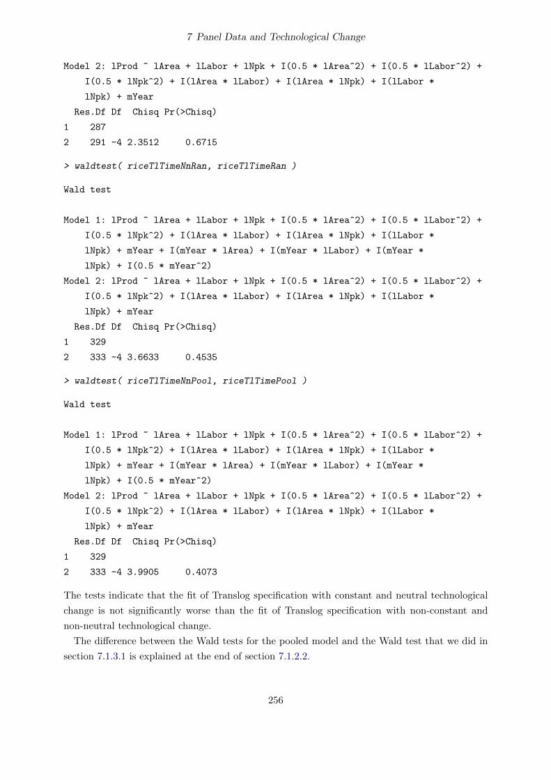
7 Panel Data and Technological Change
Model 2: lProd ~ lArea + lLabor + lNpk + I(0.5 * lArea^2) + I(0.5 * lLabor^2) +
I(0.5 * lNpk^2) + I(lArea * lLabor) + I(lArea * lNpk) + I(lLabor *
lNpk) + mYear
Res.Df Df Chisq Pr(>Chisq)
1 287
2 291 -4 2.3512 0.6715
> waldtest( riceTlTimeNnRan, riceTlTimeRan )
Wald test
Model 1: lProd ~ lArea + lLabor + lNpk + I(0.5 * lArea^2) + I(0.5 * lLabor^2) +
I(0.5 * lNpk^2) + I(lArea * lLabor) + I(lArea * lNpk) + I(lLabor *
lNpk) + mYear + I(mYear * lArea) + I(mYear * lLabor) + I(mYear *
lNpk) + I(0.5 * mYear^2)
Model 2: lProd ~ lArea + lLabor + lNpk + I(0.5 * lArea^2) + I(0.5 * lLabor^2) +
I(0.5 * lNpk^2) + I(lArea * lLabor) + I(lArea * lNpk) + I(lLabor *
lNpk) + mYear
Res.Df Df Chisq Pr(>Chisq)
1 329
2 333 -4 3.6633 0.4535
> waldtest( riceTlTimeNnPool, riceTlTimePool )
Wald test
Model 1: lProd ~ lArea + lLabor + lNpk + I(0.5 * lArea^2) + I(0.5 * lLabor^2) +
I(0.5 * lNpk^2) + I(lArea * lLabor) + I(lArea * lNpk) + I(lLabor *
lNpk) + mYear + I(mYear * lArea) + I(mYear * lLabor) + I(mYear *
lNpk) + I(0.5 * mYear^2)
Model 2: lProd ~ lArea + lLabor + lNpk + I(0.5 * lArea^2) + I(0.5 * lLabor^2) +
I(0.5 * lNpk^2) + I(lArea * lLabor) + I(lArea * lNpk) + I(lLabor *
lNpk) + mYear
Res.Df Df Chisq Pr(>Chisq)
1 329
2 333 -4 3.9905 0.4073
The tests indicate that the fit of Translog specification with constant and neutral technological
change is not significantly worse than the fit of Translog specification with non-constant and
non-neutral technological change.
The difference between the Wald tests for the pooled model and the Wald test that we did in
section 7.1.3.1 is explained at the end of section 7.1.2.2.
256

7 Panel Data and Technological Change
7.2 Frontier Production Functions with Technological Change
The frontier production technology can be estimated by many different specifications of the
stochastic frontier model. We will focus on three specifications that are all nested in the general
specification:
ln ykt = ln f(xkt, t)− ukt + vkt, (7.10)
where the subscript k = 1, . . . ,K indicates the firm, t = 1, . . . , T indicates the time period, and
all other variables are defined as before. We will apply the following three model specifications:
1. time-invariant individual efficiencies, i.e. ukt = uk, which means that each firm has an
individual fixed efficiency that does not vary over time;
2. time-variant individual efficiencies, i.e. ukt = uk exp(−η (t − T )), which means that each
firm has an individual efficiency and the efficiency terms of all firms can vary over time
with the same rate (and in the same direction); and
3. observation-specific efficiencies, i.e. no restrictions on ukt, which means that the efficiency
term of each observation is estimated independently from the other efficiencies of the firm
so that basically the panel structure of the data is ignored.
7.2.1 Cobb-Douglas Production Frontier with Technological Change
We will use the specification in equation (7.2).
7.2.1.1 Time-invariant Individual Efficiencies
We start with estimating a Cobb-Douglas production frontier with time-invariant individual
efficiencies. The following commands estimate two Cobb-Douglas production frontiers with time-
invariant individual efficiencies, the first does not account for technological change, while the
second does:
> riceCdSfaInv <- sfa( lProd ~ lArea + lLabor + lNpk, data = pdat )
> summary( riceCdSfaInv )
Error Components Frontier (see Battese & Coelli 1992)
Inefficiency decreases the endogenous variable (as in a production function)
The dependent variable is logged
Iterative ML estimation terminated after 10 iterations:
log likelihood values and parameters of two successive iterations
are within the tolerance limit
final maximum likelihood estimates
Estimate Std. Error z value Pr(>|z|)
257

7 Panel Data and Technological Change
(Intercept) 0.182630 0.035164 5.1937 2.062e-07 ***
lArea 0.453898 0.064471 7.0404 1.918e-12 ***
lLabor 0.288923 0.063856 4.5246 6.051e-06 ***
lNpk 0.227543 0.040718 5.5882 2.294e-08 ***
sigmaSq 0.155377 0.024204 6.4195 1.368e-10 ***
gamma 0.464311 0.087487 5.3072 1.113e-07 ***
---
Signif. codes: 0 ‘***’ 0.001 ‘**’ 0.01 ‘*’ 0.05 ‘.’ 0.1 ‘ ’ 1
log likelihood value: -86.43042
panel data
number of cross-sections = 43
number of time periods = 8
total number of observations = 344
thus there are 0 observations not in the panel
mean efficiency: 0.8187966
> riceCdTimeSfaInv <- sfa( lProd ~ lArea + lLabor + lNpk + mYear, data = pdat )
> summary( riceCdTimeSfaInv )
Error Components Frontier (see Battese & Coelli 1992)
Inefficiency decreases the endogenous variable (as in a production function)
The dependent variable is logged
Iterative ML estimation terminated after 11 iterations:
log likelihood values and parameters of two successive iterations
are within the tolerance limit
final maximum likelihood estimates
Estimate Std. Error z value Pr(>|z|)
(Intercept) 0.1832751 0.0345895 5.2986 1.167e-07 ***
lArea 0.4625174 0.0644245 7.1792 7.011e-13 ***
lLabor 0.3029415 0.0641323 4.7237 2.316e-06 ***
lNpk 0.2098907 0.0418709 5.0128 5.364e-07 ***
mYear 0.0116003 0.0071758 1.6166 0.106
sigmaSq 0.1556806 0.0242951 6.4079 1.475e-10 ***
gamma 0.4706143 0.0869549 5.4122 6.227e-08 ***
---
Signif. codes: 0 ‘***’ 0.001 ‘**’ 0.01 ‘*’ 0.05 ‘.’ 0.1 ‘ ’ 1
log likelihood value: -85.0743
258

7 Panel Data and Technological Change
panel data
number of cross-sections = 43
number of time periods = 8
total number of observations = 344
thus there are 0 observations not in the panel
mean efficiency: 0.8176333
In the Cobb-Douglas production frontier that accounts for technological change, the monotonicity
conditions are globally fulfilled and the (constant) output elasticities of land, labor and fertilizer
are 0.463, 0.303, and 0.21, respectively. The estimated (constant) annual rate of technological
progress is around 1.2%. However, both the t-test for the coefficient of the time trend and a
likelihood ratio test give rise to doubts whether the production technology indeed changes over
time (P-values around 10%):
> lrtest( riceCdTimeSfaInv, riceCdSfaInv )
Likelihood ratio test
Model 1: riceCdTimeSfaInv
Model 2: riceCdSfaInv
#Df LogLik Df Chisq Pr(>Chisq)
1 7 -85.074
2 6 -86.430 -1 2.7122 0.09958 .
---
Signif. codes: 0 ‘***’ 0.001 ‘**’ 0.01 ‘*’ 0.05 ‘.’ 0.1 ‘ ’ 1
Further likelihood ratio tests show that OLS models are clearly rejected in favor of the cor-
responding stochastic frontier models (no matter whether the production frontier accounts for
technological change or not):
> lrtest( riceCdSfaInv )
Likelihood ratio test
Model 1: OLS (no inefficiency)
Model 2: Error Components Frontier (ECF)
#Df LogLik Df Chisq Pr(>Chisq)
1 5 -104.91
2 6 -86.43 1 36.953 6.051e-10 ***
---
Signif. codes: 0 ‘***’ 0.001 ‘**’ 0.01 ‘*’ 0.05 ‘.’ 0.1 ‘ ’ 1
259

7 Panel Data and Technological Change
> lrtest( riceCdTimeSfaInv )
Likelihood ratio test
Model 1: OLS (no inefficiency)
Model 2: Error Components Frontier (ECF)
#Df LogLik Df Chisq Pr(>Chisq)
1 6 -104.103
2 7 -85.074 1 38.057 3.434e-10 ***
---
Signif. codes: 0 ‘***’ 0.001 ‘**’ 0.01 ‘*’ 0.05 ‘.’ 0.1 ‘ ’ 1
This model estimates only a single efficiency estimate for each of the 43 firms. Hence, the vector
returned by the efficiencies method only has 43 elements by default:
> length( efficiencies( riceCdSfaInv ) )
[1] 43
One can obtain the efficiency estimates for each observation by setting argument asInData equal
to TRUE:
> pdat$effCdInv <- efficiencies( riceCdSfaInv, asInData = TRUE )
Please note that the efficiency estimates for each firm still do not vary between time periods.
7.2.1.2 Time-variant Individual Efficiencies
Now we estimate a Cobb-Douglas production frontier with time-variant individual efficiencies.
Again, we estimate two Cobb-Douglas production frontiers, the first does not account for tech-
nological change, while the second does:
> riceCdSfaVar <- sfa( lProd ~ lArea + lLabor + lNpk,
+ timeEffect = TRUE, data = pdat )
> summary( riceCdSfaVar )
Error Components Frontier (see Battese & Coelli 1992)
Inefficiency decreases the endogenous variable (as in a production function)
The dependent variable is logged
Iterative ML estimation terminated after 11 iterations:
log likelihood values and parameters of two successive iterations
are within the tolerance limit
final maximum likelihood estimates
260

7 Panel Data and Technological Change
Estimate Std. Error z value Pr(>|z|)
(Intercept) 0.182016 0.035251 5.1635 2.424e-07 ***
lArea 0.474919 0.066213 7.1726 7.360e-13 ***
lLabor 0.300094 0.063872 4.6983 2.623e-06 ***
lNpk 0.199461 0.042740 4.6669 3.058e-06 ***
sigmaSq 0.129957 0.021098 6.1598 7.285e-10 ***
gamma 0.369639 0.104045 3.5527 0.0003813 ***
time 0.058909 0.030863 1.9087 0.0563017 .
---
Signif. codes: 0 ‘***’ 0.001 ‘**’ 0.01 ‘*’ 0.05 ‘.’ 0.1 ‘ ’ 1
log likelihood value: -84.55036
panel data
number of cross-sections = 43
number of time periods = 8
total number of observations = 344
thus there are 0 observations not in the panel
mean efficiency of each year
1 2 3 4 5 6 7 8
0.7848433 0.7950303 0.8048362 0.8142652 0.8233226 0.8320146 0.8403483 0.8483313
mean efficiency: 0.817874
> riceCdTimeSfaVar <- sfa( lProd ~ lArea + lLabor + lNpk + mYear,
+ timeEffect = TRUE, data = pdat )
> summary( riceCdTimeSfaVar )
Error Components Frontier (see Battese & Coelli 1992)
Inefficiency decreases the endogenous variable (as in a production function)
The dependent variable is logged
Iterative ML estimation terminated after 13 iterations:
log likelihood values and parameters of two successive iterations
are within the tolerance limit
final maximum likelihood estimates
Estimate Std. Error z value Pr(>|z|)
(Intercept) 0.1817471 0.0360859 5.0365 4.741e-07 ***
lArea 0.4761177 0.0657003 7.2468 4.267e-13 ***
lLabor 0.2987917 0.0647805 4.6124 3.981e-06 ***
261

7 Panel Data and Technological Change
lNpk 0.1991399 0.0428877 4.6433 3.429e-06 ***
mYear -0.0031907 0.0155009 -0.2058 0.83692
sigmaSq 0.1255592 0.0295753 4.2454 2.182e-05 ***
gamma 0.3478660 0.1507342 2.3078 0.02101 *
time 0.0711165 0.0674356 1.0546 0.29162
---
Signif. codes: 0 ‘***’ 0.001 ‘**’ 0.01 ‘*’ 0.05 ‘.’ 0.1 ‘ ’ 1
log likelihood value: -84.52871
panel data
number of cross-sections = 43
number of time periods = 8
total number of observations = 344
thus there are 0 observations not in the panel
mean efficiency of each year
1 2 3 4 5 6 7 8
0.7780285 0.7905809 0.8025753 0.8140187 0.8249202 0.8352907 0.8451431 0.8544916
mean efficiency: 0.8181311
In the Cobb-Douglas production frontier that accounts for technological change, the monotonicity
conditions are globally fulfilled and the (constant) output elasticities of land, labor and fertilizer
are 0.476, 0.299, and 0.199, respectively. The estimated (constant) annual rate of technologi-
cal change is around -0.3%, which indicates technological regress. However, the t-test for the
coefficient of the time trend and a likelihood ratio test indicate that the production technology
(frontier) does not change over time, i.e. there is neither technological regress nor technological
progress:
> lrtest( riceCdTimeSfaVar, riceCdSfaVar )
Likelihood ratio test
Model 1: riceCdTimeSfaVar
Model 2: riceCdSfaVar
#Df LogLik Df Chisq Pr(>Chisq)
1 8 -84.529
2 7 -84.550 -1 0.0433 0.8352
A positive sign of the coefficient η (named time) indicates that efficiency is increasing over
time. However, in the model without technological change, the t-test for the coefficient η and
262
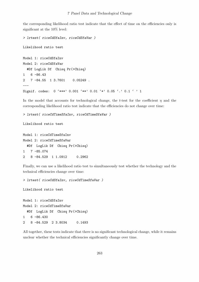
7 Panel Data and Technological Change
the corresponding likelihood ratio test indicate that the effect of time on the efficiencies only is
significant at the 10% level:
> lrtest( riceCdSfaInv, riceCdSfaVar )
Likelihood ratio test
Model 1: riceCdSfaInv
Model 2: riceCdSfaVar
#Df LogLik Df Chisq Pr(>Chisq)
1 6 -86.43
2 7 -84.55 1 3.7601 0.05249 .
---
Signif. codes: 0 ‘***’ 0.001 ‘**’ 0.01 ‘*’ 0.05 ‘.’ 0.1 ‘ ’ 1
In the model that accounts for technological change, the t-test for the coefficient η and the
corresponding likelihood ratio test indicate that the efficiencies do not change over time:
> lrtest( riceCdTimeSfaInv, riceCdTimeSfaVar )
Likelihood ratio test
Model 1: riceCdTimeSfaInv
Model 2: riceCdTimeSfaVar
#Df LogLik Df Chisq Pr(>Chisq)
1 7 -85.074
2 8 -84.529 1 1.0912 0.2962
Finally, we can use a likelihood ratio test to simultaneously test whether the technology and the
technical efficiencies change over time:
> lrtest( riceCdSfaInv, riceCdTimeSfaVar )
Likelihood ratio test
Model 1: riceCdSfaInv
Model 2: riceCdTimeSfaVar
#Df LogLik Df Chisq Pr(>Chisq)
1 6 -86.430
2 8 -84.529 2 3.8034 0.1493
All together, these tests indicate that there is no significant technological change, while it remains
unclear whether the technical efficiencies significantly change over time.
263

7 Panel Data and Technological Change
In econometric estimations of frontier models, where one variable (e.g. time) can affect both the
frontier and the efficiency, the two effects of this variable can often be hardly separated, because
the corresponding parameters can be simultaneous adjusted with only marginally reducing the
log-likelihood value. This can be checked by taking a look at the correlation matrix of the
estimated parameters:
> round( cov2cor( vcov( riceCdTimeSfaVar ) ), 2 )
(Intercept) lArea lLabor lNpk mYear sigmaSq gamma time
(Intercept) 1.00 0.18 -0.12 0.01 0.06 0.44 0.47 -0.19
lArea 0.18 1.00 -0.68 -0.39 -0.06 0.04 0.06 0.07
lLabor -0.12 -0.68 1.00 -0.27 0.08 -0.07 -0.09 0.00
lNpk 0.01 -0.39 -0.27 1.00 0.01 0.02 0.00 -0.11
mYear 0.06 -0.06 0.08 0.01 1.00 0.71 0.70 -0.88
sigmaSq 0.44 0.04 -0.07 0.02 0.71 1.00 0.94 -0.85
gamma 0.47 0.06 -0.09 0.00 0.70 0.94 1.00 -0.85
time -0.19 0.07 0.00 -0.11 -0.88 -0.85 -0.85 1.00
The estimate of the parameter for technological change (mYear) is highly correlated with the
estimate of the parameter that indicates the change of the efficiencies (time).
Again, further likelihood ratio tests show that OLS models are clearly rejected in favor of the
corresponding stochastic frontier models:
> lrtest( riceCdSfaVar )
Likelihood ratio test
Model 1: OLS (no inefficiency)
Model 2: Error Components Frontier (ECF)
#Df LogLik Df Chisq Pr(>Chisq)
1 5 -104.91
2 7 -84.55 2 40.713 4.489e-10 ***
---
Signif. codes: 0 ‘***’ 0.001 ‘**’ 0.01 ‘*’ 0.05 ‘.’ 0.1 ‘ ’ 1
> lrtest( riceCdTimeSfaVar )
Likelihood ratio test
Model 1: OLS (no inefficiency)
Model 2: Error Components Frontier (ECF)
#Df LogLik Df Chisq Pr(>Chisq)
264

7 Panel Data and Technological Change
1 6 -104.103
2 8 -84.529 2 39.149 9.85e-10 ***
---
Signif. codes: 0 ‘***’ 0.001 ‘**’ 0.01 ‘*’ 0.05 ‘.’ 0.1 ‘ ’ 1
In case of time-variant efficiencies, the efficiencies method returns a matrix, where each row
corresponds to one of the 43 firms and each column corresponds to one of the 0 time periods:
> dim( efficiencies( riceCdSfaVar ) )
[1] 43 8
One can obtain a vector of efficiency estimates for each observation by setting argument asInData
equal to TRUE:
> pdat$effCdVar <- efficiencies( riceCdSfaVar, asInData = TRUE )
7.2.1.3 Observation-specific efficiencies
Finally, we estimate a Cobb-Douglas production frontier with observation-specific efficiencies.
The following commands estimate two Cobb-Douglas production frontiers, the first does not
account for technological change, while the second does:
> riceCdSfa <- sfa( lProd ~ lArea + lLabor + lNpk, data = riceProdPhil )
> summary( riceCdSfa )
Error Components Frontier (see Battese & Coelli 1992)
Inefficiency decreases the endogenous variable (as in a production function)
The dependent variable is logged
Iterative ML estimation terminated after 9 iterations:
log likelihood values and parameters of two successive iterations
are within the tolerance limit
final maximum likelihood estimates
Estimate Std. Error z value Pr(>|z|)
(Intercept) 0.333747 0.024468 13.6400 < 2.2e-16 ***
lArea 0.355511 0.060125 5.9128 3.363e-09 ***
lLabor 0.333302 0.063026 5.2883 1.234e-07 ***
lNpk 0.271277 0.035364 7.6709 1.708e-14 ***
sigmaSq 0.238627 0.025941 9.1987 < 2.2e-16 ***
gamma 0.885382 0.033524 26.4103 < 2.2e-16 ***
---
Signif. codes: 0 ‘***’ 0.001 ‘**’ 0.01 ‘*’ 0.05 ‘.’ 0.1 ‘ ’ 1
265
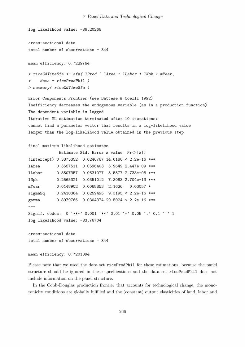
7 Panel Data and Technological Change
log likelihood value: -86.20268
cross-sectional data
total number of observations = 344
mean efficiency: 0.7229764
> riceCdTimeSfa <- sfa( lProd ~ lArea + lLabor + lNpk + mYear,
+ data = riceProdPhil )
> summary( riceCdTimeSfa )
Error Components Frontier (see Battese & Coelli 1992)
Inefficiency decreases the endogenous variable (as in a production function)
The dependent variable is logged
Iterative ML estimation terminated after 10 iterations:
cannot find a parameter vector that results in a log-likelihood value
larger than the log-likelihood value obtained in the previous step
final maximum likelihood estimates
Estimate Std. Error z value Pr(>|z|)
(Intercept) 0.3375352 0.0240787 14.0180 < 2.2e-16 ***
lArea 0.3557511 0.0596403 5.9649 2.447e-09 ***
lLabor 0.3507357 0.0631077 5.5577 2.733e-08 ***
lNpk 0.2565321 0.0351012 7.3083 2.704e-13 ***
mYear 0.0148902 0.0068853 2.1626 0.03057 *
sigmaSq 0.2418364 0.0259495 9.3195 < 2.2e-16 ***
gamma 0.8979766 0.0304374 29.5024 < 2.2e-16 ***
---
Signif. codes: 0 ‘***’ 0.001 ‘**’ 0.01 ‘*’ 0.05 ‘.’ 0.1 ‘ ’ 1
log likelihood value: -83.76704
cross-sectional data
total number of observations = 344
mean efficiency: 0.7201094
Please note that we used the data set riceProdPhil for these estimations, because the panel
structure should be ignored in these specifications and the data set riceProdPhil does not
include information on the panel structure.
In the Cobb-Douglas production frontier that accounts for technological change, the mono-
tonicity conditions are globally fulfilled and the (constant) output elasticities of land, labor and
266

7 Panel Data and Technological Change
fertilizer are 0.356, 0.351, and 0.257, respectively. The estimated (constant) annual rate of tech-
nological change is around 1.5%.
A likelihood ratio test confirms the t-test for the coefficient of the time trend, i.e. the production
technology significantly changes over time:
> lrtest( riceCdTimeSfa, riceCdSfa )
Likelihood ratio test
Model 1: riceCdTimeSfa
Model 2: riceCdSfa
#Df LogLik Df Chisq Pr(>Chisq)
1 7 -83.767
2 6 -86.203 -1 4.8713 0.02731 *
---
Signif. codes: 0 ‘***’ 0.001 ‘**’ 0.01 ‘*’ 0.05 ‘.’ 0.1 ‘ ’ 1
7.2.2 Translog Production Frontier with Constant and Neutral Technological
Change
The specification of a Translog production function that accounts for constant and neutral (un-
biased) technological change is given in (7.4).1
7.2.2.1 Observation-Specific Efficiencies
The following commands estimate a two Translog production frontiers with observation-specific
efficiencies, the first does not account for technological change, while the second can account for
constant and neutral technical change:
> riceTlSfa <- sfa( log( prod ) ~ log( area ) + log( labor ) + log( npk ) +
+ I( 0.5 * log( area )^2 ) + I( 0.5 * log( labor )^2 ) + I( 0.5 * log( npk )^2 ) +
+ I( log( area ) * log( labor ) ) + I( log( area ) * log( npk ) ) +
+ I( log( labor ) * log( npk ) ), data = riceProdPhil )
> summary( riceTlSfa )
Error Components Frontier (see Battese & Coelli 1992)
Inefficiency decreases the endogenous variable (as in a production function)
The dependent variable is logged
Iterative ML estimation terminated after 16 iterations:
1We use not only mean-scaled input quantities but also the mean-scaled output quantity in order to obtainthe same estimates as Coelli et al. (2005, p. 250). Please note that the order of coefficients/regressors isdifferent in Coelli et al. (2005, p. 250): intercept, mYear, log(area), log(labor), log(npk), 0.5*log(area)^2,log(area)*log(labor), log(area)*log(npk), 0.5*log(labor)^2, log(labor)*log(npk), 0.5*log(npk)^2.
267

7 Panel Data and Technological Change
log likelihood values and parameters of two successive iterations
are within the tolerance limit
final maximum likelihood estimates
Estimate Std. Error z value Pr(>|z|)
(Intercept) 3.3719e-01 2.8747e-02 11.7298 < 2.2e-16 ***
log(area) 5.3429e-01 7.9139e-02 6.7513 1.466e-11 ***
log(labor) 2.0910e-01 7.4439e-02 2.8090 0.0049699 **
log(npk) 2.2145e-01 4.5141e-02 4.9057 9.309e-07 ***
I(0.5 * log(area)^2) -5.1502e-01 2.0692e-01 -2.4889 0.0128124 *
I(0.5 * log(labor)^2) -5.6134e-01 2.7039e-01 -2.0761 0.0378885 *
I(0.5 * log(npk)^2) -7.1029e-05 9.4128e-02 -0.0008 0.9993979
I(log(area) * log(labor)) 6.2604e-01 1.7284e-01 3.6221 0.0002922 ***
I(log(area) * log(npk)) 8.1749e-02 1.3867e-01 0.5895 0.5555218
I(log(labor) * log(npk)) -1.5750e-01 1.4027e-01 -1.1228 0.2615321
sigmaSq 2.1856e-01 2.4990e-02 8.7458 < 2.2e-16 ***
gamma 8.6930e-01 3.9456e-02 22.0319 < 2.2e-16 ***
---
Signif. codes: 0 ‘***’ 0.001 ‘**’ 0.01 ‘*’ 0.05 ‘.’ 0.1 ‘ ’ 1
log likelihood value: -76.95413
cross-sectional data
total number of observations = 344
mean efficiency: 0.7326115
> riceTlTimeSfa <- sfa( log( prod ) ~ log( area ) + log( labor ) + log( npk ) +
+ I( 0.5 * log( area )^2 ) + I( 0.5 * log( labor )^2 ) + I( 0.5 * log( npk )^2 ) +
+ I( log( area ) * log( labor ) ) + I( log( area ) * log( npk ) ) +
+ I( log( labor ) * log( npk ) ) + mYear, data = riceProdPhil )
> summary( riceTlTimeSfa )
Error Components Frontier (see Battese & Coelli 1992)
Inefficiency decreases the endogenous variable (as in a production function)
The dependent variable is logged
Iterative ML estimation terminated after 17 iterations:
log likelihood values and parameters of two successive iterations
are within the tolerance limit
final maximum likelihood estimates
268

7 Panel Data and Technological Change
Estimate Std. Error z value Pr(>|z|)
(Intercept) 0.3423626 0.0285089 12.0090 < 2.2e-16 ***
log(area) 0.5313816 0.0786313 6.7579 1.400e-11 ***
log(labor) 0.2308950 0.0744167 3.1027 0.0019174 **
log(npk) 0.2032741 0.0448189 4.5355 5.748e-06 ***
I(0.5 * log(area)^2) -0.4758612 0.2021533 -2.3540 0.0185745 *
I(0.5 * log(labor)^2) -0.5644708 0.2652593 -2.1280 0.0333374 *
I(0.5 * log(npk)^2) -0.0072200 0.0923371 -0.0782 0.9376756
I(log(area) * log(labor)) 0.6088402 0.1658019 3.6721 0.0002406 ***
I(log(area) * log(npk)) 0.0617400 0.1383298 0.4463 0.6553627
I(log(labor) * log(npk)) -0.1370538 0.1407360 -0.9738 0.3301377
mYear 0.0151111 0.0069164 2.1848 0.0289024 *
sigmaSq 0.2217092 0.0251305 8.8223 < 2.2e-16 ***
gamma 0.8835549 0.0367095 24.0688 < 2.2e-16 ***
---
Signif. codes: 0 ‘***’ 0.001 ‘**’ 0.01 ‘*’ 0.05 ‘.’ 0.1 ‘ ’ 1
log likelihood value: -74.40992
cross-sectional data
total number of observations = 344
mean efficiency: 0.7294192
In the Translog production frontier that accounts for constant and neutral technological change,
the monotonicity conditions are fulfilled at the sample mean and the estimated output elasticities
of land, labor and fertilizer are 0.531, 0.231, and 0.203, respectively, at the sample mean. The
estimated (constant) annual rate of technological progress is around 1.5%. A likelihood ratio test
confirms the t-test for the coefficient of the time trend, i.e. the production technology (frontier)
significantly changes over time:
> lrtest( riceTlTimeSfa, riceTlSfa )
Likelihood ratio test
Model 1: riceTlTimeSfa
Model 2: riceTlSfa
#Df LogLik Df Chisq Pr(>Chisq)
1 13 -74.410
2 12 -76.954 -1 5.0884 0.02409 *
---
Signif. codes: 0 ‘***’ 0.001 ‘**’ 0.01 ‘*’ 0.05 ‘.’ 0.1 ‘ ’ 1
269

7 Panel Data and Technological Change
Two further likelihood ratio tests indicate that the Translog specification is superior to the Cobb-
Douglas specification, no matter whether the two models allow for technological change or not.
> lrtest( riceTlSfa, riceCdSfa )
Likelihood ratio test
Model 1: riceTlSfa
Model 2: riceCdSfa
#Df LogLik Df Chisq Pr(>Chisq)
1 12 -76.954
2 6 -86.203 -6 18.497 0.005103 **
---
Signif. codes: 0 ‘***’ 0.001 ‘**’ 0.01 ‘*’ 0.05 ‘.’ 0.1 ‘ ’ 1
> lrtest( riceTlTimeSfa, riceCdTimeSfa )
Likelihood ratio test
Model 1: riceTlTimeSfa
Model 2: riceCdTimeSfa
#Df LogLik Df Chisq Pr(>Chisq)
1 13 -74.410
2 7 -83.767 -6 18.714 0.004674 **
---
Signif. codes: 0 ‘***’ 0.001 ‘**’ 0.01 ‘*’ 0.05 ‘.’ 0.1 ‘ ’ 1
7.2.3 Translog Production Frontier with Non-Constant and Non-Neutral
Technological Change
The specification of a Translog production function with non-Constant and non-Neutral techno-
logical change is given in (7.7).
7.2.3.1 Observation-Specific Efficiencies
The following command estimates a Translog production frontier with observation-specific effi-
ciencies that can account for non-constant rates of technological change as well as biased techno-
logical change:
> riceTlTimeNnSfa <- sfa( log( prod ) ~ log( area ) + log( labor ) + log( npk ) +
+ I( 0.5 * log( area )^2 ) + I( 0.5 * log( labor )^2 ) + I( 0.5 * log( npk )^2 ) +
+ I( log( area ) * log( labor ) ) + I( log( area ) * log( npk ) ) +
+ I( log( labor ) * log( npk ) ) + mYear + I( mYear * log( area ) ) +
270
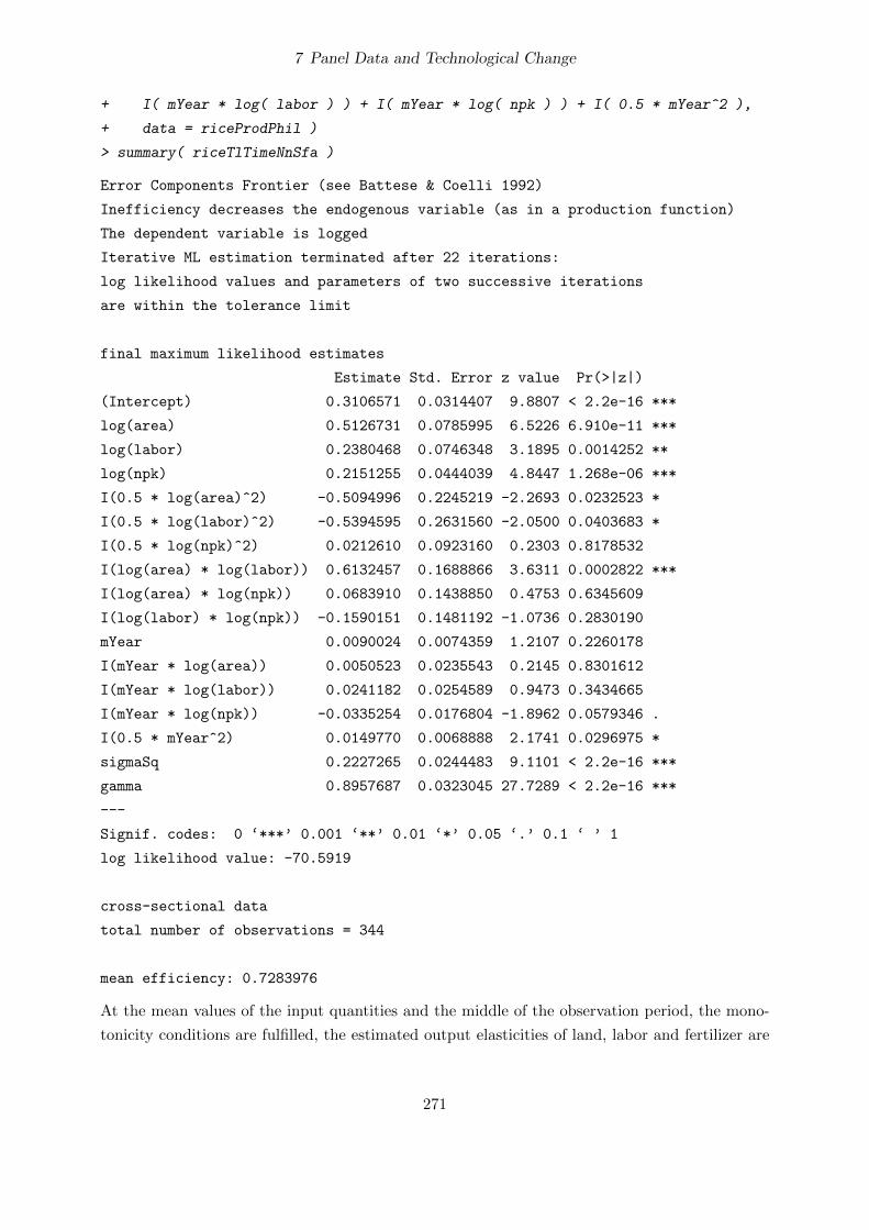
7 Panel Data and Technological Change
+ I( mYear * log( labor ) ) + I( mYear * log( npk ) ) + I( 0.5 * mYear^2 ),
+ data = riceProdPhil )
> summary( riceTlTimeNnSfa )
Error Components Frontier (see Battese & Coelli 1992)
Inefficiency decreases the endogenous variable (as in a production function)
The dependent variable is logged
Iterative ML estimation terminated after 22 iterations:
log likelihood values and parameters of two successive iterations
are within the tolerance limit
final maximum likelihood estimates
Estimate Std. Error z value Pr(>|z|)
(Intercept) 0.3106571 0.0314407 9.8807 < 2.2e-16 ***
log(area) 0.5126731 0.0785995 6.5226 6.910e-11 ***
log(labor) 0.2380468 0.0746348 3.1895 0.0014252 **
log(npk) 0.2151255 0.0444039 4.8447 1.268e-06 ***
I(0.5 * log(area)^2) -0.5094996 0.2245219 -2.2693 0.0232523 *
I(0.5 * log(labor)^2) -0.5394595 0.2631560 -2.0500 0.0403683 *
I(0.5 * log(npk)^2) 0.0212610 0.0923160 0.2303 0.8178532
I(log(area) * log(labor)) 0.6132457 0.1688866 3.6311 0.0002822 ***
I(log(area) * log(npk)) 0.0683910 0.1438850 0.4753 0.6345609
I(log(labor) * log(npk)) -0.1590151 0.1481192 -1.0736 0.2830190
mYear 0.0090024 0.0074359 1.2107 0.2260178
I(mYear * log(area)) 0.0050523 0.0235543 0.2145 0.8301612
I(mYear * log(labor)) 0.0241182 0.0254589 0.9473 0.3434665
I(mYear * log(npk)) -0.0335254 0.0176804 -1.8962 0.0579346 .
I(0.5 * mYear^2) 0.0149770 0.0068888 2.1741 0.0296975 *
sigmaSq 0.2227265 0.0244483 9.1101 < 2.2e-16 ***
gamma 0.8957687 0.0323045 27.7289 < 2.2e-16 ***
---
Signif. codes: 0 ‘***’ 0.001 ‘**’ 0.01 ‘*’ 0.05 ‘.’ 0.1 ‘ ’ 1
log likelihood value: -70.5919
cross-sectional data
total number of observations = 344
mean efficiency: 0.7283976
At the mean values of the input quantities and the middle of the observation period, the mono-
tonicity conditions are fulfilled, the estimated output elasticities of land, labor and fertilizer are
271

7 Panel Data and Technological Change
0.513, 0.238, and 0.215, respectively, and the estimated annual rate of technological progress is
around 0.9%.
The following likelihood ratio tests compare the Translog production frontier that can account
for non-constant rates of technological change as well as biased technological change with the
Translog production frontier that does not account for technological change and with the Translog
production frontier that only accounts for constant and neutral technological change:
> lrtest( riceTlTimeNnSfa, riceTlSfa )
Likelihood ratio test
Model 1: riceTlTimeNnSfa
Model 2: riceTlSfa
#Df LogLik Df Chisq Pr(>Chisq)
1 17 -70.592
2 12 -76.954 -5 12.725 0.0261 *
---
Signif. codes: 0 ‘***’ 0.001 ‘**’ 0.01 ‘*’ 0.05 ‘.’ 0.1 ‘ ’ 1
> lrtest( riceTlTimeNnSfa, riceTlTimeSfa )
Likelihood ratio test
Model 1: riceTlTimeNnSfa
Model 2: riceTlTimeSfa
#Df LogLik Df Chisq Pr(>Chisq)
1 17 -70.592
2 13 -74.410 -4 7.636 0.1059
These tests indicate that the Translog production frontier that can account for non-constant
rates of technological change as well as biased technological change is superior to the Translog
production frontier that does not account for any technological change but it is not significantly
better than the Translog production frontier that accounts for constant and neutral technological
change. Although it seems to be unnecessary to use the Translog production frontier that can
account for non-constant rates of technological change as well as biased technological change, we
use it in our further analysis for demonstrative purposes.
The following commands create short-cuts for some of the estimated coefficients and calculate
the rates of technological change at each observation:
> at <- coef(riceTlTimeNnSfa)["mYear"]
> atArea <- coef(riceTlTimeNnSfa)["I(mYear * log(area))"]
> atLabor <- coef(riceTlTimeNnSfa)["I(mYear * log(labor))"]
272

7 Panel Data and Technological Change
> atNpk <- coef(riceTlTimeNnSfa)["I(mYear * log(npk))"]
> att <- coef(riceTlTimeNnSfa)["I(0.5 * mYear^2)"]
> riceProdPhil$tc <- with( riceProdPhil, at + atArea * log( area ) +
+ atLabor * log( labor ) + atNpk * log( npk ) + att * mYear )
The following command visualizes the variation of the individual rates of technological change:
> hist( riceProdPhil$tc, 20 )
technological change
Fre
quen
cy
−0.05 0.00 0.05 0.10
010
30
Figure 7.3: Annual rates of technological change
The resulting graph is shown in figure 7.3. Most individual rates of technological change are
between −4% and +7%, i.e. there is technological regress at some observations, while there
is strong technological progress at other observations. This wide variation of annual rates of
technological change is not unusual in applied agricultural production analysis because of the
stochastic nature of agricultural production.
7.2.4 Decomposition of Productivity Growth
In the beginning of this course, we have discussed and calculated different productivity mea-
sures, of which the total factor productivity (TFP ) is a particularly important determinant of a
firm’s competitiveness. During this course, we have—amongst other things—analyzed all three
measures that affect a firm’s total factor productivity, i.e.
� the current state of the technology (T ) in the firm’s sector, which might change due to
technological change,
� the firm’s technical efficiency (TE), which might change if the firm’s distance to the current
technology changes, and
� the firm’s scale efficiency (SE), which might change if the firm’s size relative to the optimal
firm size changes.
Hence, changes of a firm’s (or a sector’s) total factor productivity (∆TFP ) can be decom-
posed into technological changes (∆T ), technical efficiency changes (∆TE), and scale efficiency
273

7 Panel Data and Technological Change
changes (∆SE):
∆TFP ≈ ∆T + ∆TE + ∆SE (7.11)
This decomposition often helps to understand the reasons for improved or reduced total factor
productivity and competitiveness.
7.3 Analysing Productivity Growths with Data Envelopment Analysis
(DEA)
> library( "Benchmarking" )
We create a matrix of input quantities and a vector of output quantities:
> xMat <- cbind( riceProdPhil$AREA, riceProdPhil$LABOR, riceProdPhil$NPK )
> yVec <- riceProdPhil$PROD
The following commands calculate and decompose productivity changes:
> xMat0 <- xMat[ riceProdPhil$YEARDUM == 1, ]
> xMat1 <- xMat[ riceProdPhil$YEARDUM == 2, ]
> yVec0 <- yVec[ riceProdPhil$YEARDUM == 1 ]
> yVec1 <- yVec[ riceProdPhil$YEARDUM == 2 ]
> c00 <- eff( dea( xMat0, yVec0, RTS = "crs" ) )
> c01 <- eff( dea( xMat0, yVec0, XREF = xMat1, YREF = yVec1, RTS = "crs" ) )
> c11 <- eff( dea( xMat1, yVec1, RTS = "crs" ) )
> c10 <- eff( dea( xMat1, yVec1, XREF = xMat0, YREF = yVec0, RTS = "crs" ) )
Productivity changes (Malmquist):
> dProd0 <- c10 / c00
> hist( dProd0 )
> dProd1 <- c11 / c01
> plot( dProd0, dProd1 )
> dProd <- sqrt( dProd0 * dProd1 )
> hist( dProd )
Technological changes:
> dTech0 <- c00 / c01
> dTech1 <- c10 / c11
> plot( dTech0, dTech1 )
> dTech <- sqrt( dTech0 * dTech1 )
> hist( dTech )
274

7 Panel Data and Technological Change
Efficiency changes:
> dEff <- c11 / c00
> hist( dEff )
Checking Malmquist decomposition:
> all.equal( dProd, dTech * dEff )
[1] TRUE
275

Bibliography
Aigner, D., C.A.K. Lovell, and P. Schmidt. 1977. “Formulation and Estimation of Stochastic
Frontier Production Function Models.” Journal of Econometrics 6:21–37.
Battese, G.E., and T.J. Coelli. 1995. “A Model for Technical Inefficiency Effects in a Stochastic
Frontier Production Function for Panel Data.” Empirical Economics 20:325–332.
Bogetoft, P., and L. Otto. 2011. Benchmarking with DEA, SFA, and R, vol. 157 of International
Series in Operations Research & Management Science. Springer.
Chambers, R.G. 1988. Applied Production Analysis. A Dual Approach. Cambridge University
Press, Cambridge.
Chand, R., and J.L. Kaul. 1986. “A Note on the Use of the Cobb-Douglas Profit Function.”
American Journal of Agricultural Economics 68:162–164.
Chiang, A.C. 1984. Fundamental Methods of Mathematical Economics, 3rd ed. McGraw-Hill.
Coelli, T.J. 1995. “Estimators and Hypothesis Tests for a Stochastic: A Monte Carlo Analysis.”
Journal of Productivity Analysis 6:247–268.
Coelli, T.J., D.S.P. Rao, C.J. O’Donnell, and G.E. Battese. 2005. An Introduction to Efficiency
and Productivity Analysis, 2nd ed. New York: Springer.
Croissant, Y., and G. Millo. 2008. “Panel Data Econometrics in R: The plm Package.” Journal
of Statistical Software 27:1–43.
Czekaj, T., and A. Henningsen. 2012. “Comparing Parametric and Nonparametric Regression
Methods for Panel Data: the Optimal Size of Polish Crop Farms.” FOI Working Paper No.
2012/12, Institute of Food and Resource Economics, University of Copenhagen.
Hayfield, T., and J.S. Racine. 2008. “Nonparametric Econometrics: The np Package.” Journal of
Statistical Software 27:1–32.
Henning, C.H.C.A., and A. Henningsen. 2007. “Modeling Farm Households’ Price Responses in
the Presence of Transaction Costs and Heterogeneity in Labor Markets.” American Journal of
Agricultural Economics 89:665–681.
276

Bibliography
Hurvich, C.M., J.S. Simonoff, and C.L. Tsai. 1998. “Smooting Parameter Selection in Nonpara-
metric Regression Using an Improved Akaike Information Criterion.” Journal of the Royal
Statistical Society Series B 60:271–293.
Ivaldi, M., N. Ladoux, H. Ossard, and M. Simioni. 1996. “Comparing Fourier and Translog
Specifications of Multiproduct Technology: Evidence from an Incomplete Panel of French
Farmers.” Journal of Applied Econometrics 11:649–667.
Kleiber, C., and A. Zeileis. 2008. Applied Econometrics with R. New York: Springer.
Li, Q., and J.S. Racine. 2007. Nonparametric Econometrics: Theory and Practice. Princeton:
Princeton University Press.
McClelland, J.W., M.E. Wetzstein, and W.N. Musserwetz. 1986. “Returns to Scale and Size in
Agricultural Economics.” Western Journal of Agricultural Economics 11:129–133.
Meeusen, W., and J. van den Broeck. 1977.“Efficiency Estimation from Cobb-Douglas Production
Functions with Composed Error.” International Economic Review 18:435–444.
Olsen, J.V., and A. Henningsen. 2011. “Investment Utilization and Farm Efficiency in Danish
Agriculture.” FOI Working Paper No. 2011/13, Institute of Food and Resource Economics,
University of Copenhagen.
Racine, J.S. 2008. “Nonparametric Econometrics: A Primer.” Foundations and Trends in Econo-
metrics 3:1–88.
Teetor, P. 2011. R Cookbook . O’Reilly Media.
Zuur, A., E.N. Ieno, and E. Meesters. 2009. A Beginner’s Guide to R. Use R!, Springer.
277