introduction to factor analysis for marketing - skim...
TRANSCRIPT
Introduction to Factor Analysis for MarketingSKIM/Sawtooth Software Conference 2016, Rome
Chris Chapman, Google. April 2016.
Special thanks to Josh Lewandowski at Google for helpfulfeedback (errors are mine!)

1 Introduction
2 Exploratory Factor Analysis
3 Does rotation work? Comparisons
4 Break!
5 Confirmatory Factor Analysis
6 Finally

Introduction

Overview
This presentation is primarily a conceptual introduction to factoranalysis. We will focus more on concepts and best practices than ontechnical details.
Motivation & BasicsExploratory Factor Analysis (EFA)Confirmatory Factor Analysis (CFA)Further Learning
Examples are shown in R, but the process and results are similar inSPSS and other statistics packages.
Motivation: Example
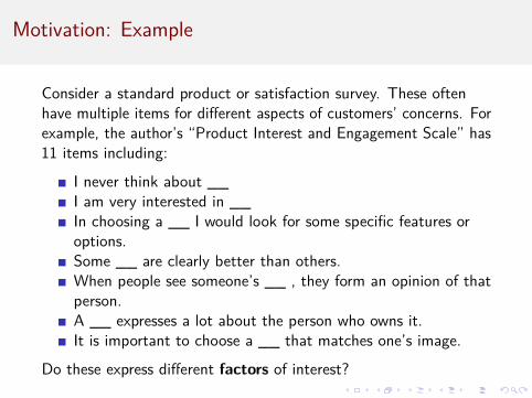
Consider a standard product or satisfaction survey. These oftenhave multiple items for different aspects of customers’ concerns. Forexample, the author’s “Product Interest and Engagement Scale” has11 items including:
I never think about __I am very interested in __In choosing a __ I would look for some specific features oroptions.Some __ are clearly better than others.When people see someone’s __ , they form an opinion of thatperson.A __ expresses a lot about the person who owns it.It is important to choose a __ that matches one’s image.
Do these express different factors of interest?

Exploratory Factor Analysis

The General Concept (version 1)
From the original variables, factor analysis (FA) tries to find asmaller number of derived variables (factors) that meet theseconditions:
1 Maximally capture the correlations among the original variables(after accounting for error)
2 Each factor is associated clearly with a subset of the variables3 Each variable is associated clearly with (ideally) only one factor4 The factors are maximally differentiated from one another
These are rarely met perfectly in practice, but when they areapproximated, the solution is close to “simple structure” that is veryinterpretable.

The General Concept, version 1 example
Consider (fictonal) factor analysis of a standardized school test:
Variable Factor 1 Factor 2 Factor 3
Arithmetic score 0.45 0.88 0.25Algebra score 0.51 0.82 0.03Logic score 0.41 0.50 0.11Puzzle score 0.25 0.42 0.07Vocabulary score 0.43 0.09 0.93Reading score 0.50 0.14 0.85
We might interpret this as showing:
Factor 1: general aptitudeFactor 2: mathematical skillsFactor 3: language skills

The General Concept in Simplified Math
In short: the factor loading matrix, times itself (its own transpose),closely recreates the variable-variable covariance matrix.
LL′(+E ) = C
LoadingsLoadings ′(+Error) = CovarianceF1.v1 F2.v1F1.v2 F2.v2F1.v3 F2.v3
[F1.v1 F1.v2 F1.v3F1.v2 F2.v2 F2.v3
]=
v1.v1 v1.v2 v1.v3v2.v1 v2.v2 v2.v3v3.v1 v3.v2 v3.v3

The General Concept (version 2)
Another way to look at FA is that it seeks latent variables. A latentvariable is an unobservable data generating process — such as amental state — that is manifested in measurable quantities (such assurvey items).The product interest survey was designed to assess three latentvariables:
General interest in a product categoryDetailed interest in specific featuresInterest in the product as an “image” product
Each of those is assessed with multiple items because any singleitem is imperfect.

Visual Example for Product Interest
i1 i2 i3 i4 i5 i6 i7 i8 i9 i10 i11
Gnr Ftr Img

Very Different Modes of Factor Analysis
Exploratory Factor Analysis (EFA)
Asks what the factors are in observed dataRequires interpretation of usefulnessBefore assuming it’s correct, confirm with CFA
Confirmatory Factor Analysis (CFA)
Asks how well a proposed model fits given dataIs a flavor of structural equation modeling (SEM)Doesn’t give an absolute answer; should compare models
Key terms and symbols
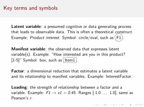
Latent variable: a presumed cognitive or data generating processthat leads to observable data. This is often a theoretical construct.Example: Product interest. Symbol: circle/oval, such as F1 .
Manifest variable: the observed data that expresses latentvariable(s). Example: “How interested are you in this product?[1-5]” Symbol: box, such as Item1 .
Factor: a dimensional reduction that estimates a latent variableand its relationship to manifest variables. Example: InterestFactor.
Loading: the strength of relationship between a factor and avariable. Example: F1 → v1 = 0.45. Ranges [-1.0 . . . 1.0], same asPearson’s r.

Visual model, again
i1 i2 i3 i4 i5 i6 i7 i8 i9 i10 i11
Gnr Ftr Img

EFA vs Principal Components
Factor analysis is often advantageous over PCA because:- It’s more interpretable; FA aims for clear factor/variablerelationships- FA does this by mathematically rotating the components to haveclearer loadings (and by omitting non-shared “error” variance)- FA estimates latent variables in presence of error
Principal components is advantageous when:- You want an exact reduction of the data regardless of error- You want to maximize variance explained by the first Kcomponents

General Steps for EFA
1 Load and clean the data. Put it on a common scale (e.g.,standardize) and address extreme skew.
2 Examine correlation matrix to get a sense of possible factors3 Determine the number of factors4 Choose a factor rotation model (more in a moment)5 Fit the model and interpret the resulting factors6 Repeat 3-5 if unclear, and select the most useful7 Use factor scores for best estimate of construct/latent variable

Now . . . data!
11 items for simulated product interest and engagement data(PIES), rated on 7 point Likert type scale. We will determine theright number of factors and their variable loadings.
Items:
Paraphrased item
not important [reversed] never think [reversed]very interested look for specific featuresinvestigate in depth some are clearly betterlearn about options others see, form opinionexpresses person tells about personmatch one’s image

Step 1: Load and clean data
pies.data <- read.csv("http://goo.gl/yT0XwJ")
## vars n mean sd median trimmed mad min max range## NotImportant 1 3600 4.34 1.00 4 4.32 1.48 1 7 6## NeverThink 2 3600 4.10 1.05 4 4.09 1.48 1 7 6## VeryInterested 3 3600 4.11 1.02 4 4.10 1.48 1 7 6## LookFeatures 4 3600 4.04 1.05 4 4.04 1.48 1 7 6## InvestigateDepth 5 3600 4.00 1.08 4 4.00 1.48 1 7 6## SomeAreBetter 6 3600 3.92 1.04 4 3.94 1.48 1 7 6## LearnAboutOptions 7 3600 3.87 1.04 4 3.88 1.48 1 7 6## OthersOpinion 8 3600 3.90 1.11 4 3.92 1.48 1 7 6## ExpressesPerson 9 3600 4.02 1.01 4 4.01 1.48 1 7 6## TellsAbout 10 3600 3.90 1.02 4 3.92 1.48 1 7 6## MatchImage 11 3600 3.85 1.01 4 3.86 1.48 1 7 6## skew kurtosis se## NotImportant -0.07 -0.01 0.02## NeverThink -0.01 -0.07 0.02## VeryInterested -0.01 -0.13 0.02## LookFeatures -0.07 -0.05 0.02## InvestigateDepth -0.02 -0.07 0.02## SomeAreBetter -0.08 0.02 0.02## LearnAboutOptions 0.02 -0.10 0.02## OthersOpinion 0.02 -0.12 0.02## ExpressesPerson 0.07 -0.05 0.02## TellsAbout -0.04 0.05 0.02## MatchImage 0.01 -0.01 0.02
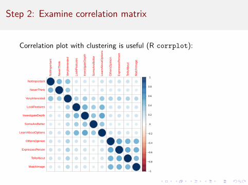
Step 2: Examine correlation matrix
Correlation plot with clustering is useful (R corrplot):
−1
−0.8
−0.6
−0.4
−0.2
0
0.2
0.4
0.6
0.8
1
Not
Impo
rtan
t
Nev
erT
hink
Ver
yInt
eres
ted
Look
Fea
ture
s
Inve
stig
ateD
epth
Som
eAre
Bet
ter
Lear
nAbo
utO
ptio
ns
Oth
ersO
pini
on
Exp
ress
esP
erso
n
Tells
Abo
ut
Mat
chIm
age
NotImportant
NeverThink
VeryInterested
LookFeatures
InvestigateDepth
SomeAreBetter
LearnAboutOptions
OthersOpinion
ExpressesPerson
TellsAbout
MatchImage

Step 3: Determine number of factors (1)
There is usually not a definitive answer. Choosing number of factorsis partially a matter of usefulness.
Generally, look for consensus among:- Theory: how many do you expect?- Correlation matrix: how many seem to be there?- Eigenvalues: how many Factors have Eigenvalue > 1?- Eigenvalue scree plot: where is the “bend” in extraction?- Parallel analysis and acceleration [advanced; less used; not coveredtoday]

Step 3: Number of factors: Eigenvalues
In factor analysis, an eigenvalue is the proportion of total shared(i.e., non-error) variance explained by each factor. You might thinkof it as volume in multidimensional space, where each variable adds1.0 to the volume (thus, sum(eigenvalues) = # of variables).
A factor is only useful if it explains more than 1 variable . . . andthus has eigenvalue > 1.0.
eigen(cor(pies.data))$values
## [1] 3.6606016 1.6422691 1.2749132 0.6880529 0.5800595 0.5719967 0.5607506## [8] 0.5387749 0.5290039 0.4834441 0.4701335
This rule of thumb suggests 3 factors for the present data.

Step 3: Eigenvalue scree plot
prcomp(pies.data)
Var
ianc
es
0.5
1.0
1.5
2.0
2.5
3.0
3.5
4.0
1 2 3 4 5 6 7 8 9 10

Step 4: Choose a factor rotation model
EFA can be thought of as slicing a pizza. The same material(variance) can be carved up in ways that are mathematicallyidentical, but might be more or less useful for a given situation.
Key decision: do you want the extracted factors to be correlated ornot? In FA jargon, orthogonal or oblique?
By default, EFA looks for orthogonal factors that have r=0correlation. This maximizes the interpretability, so I recommendusing an orthogonal rotation in most cases, at least to start. (Asa practical matter, it often makes little difference.)
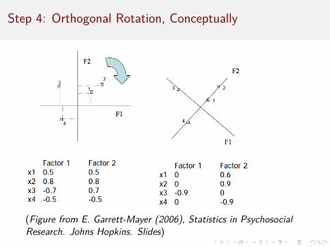
Step 4: Orthogonal Rotation, Conceptually
(Figure from E. Garrett-Mayer (2006), Statistics in PsychosocialResearch. Johns Hopkins. Slides)
Step 4: Some rotation options
Default: varimax: orthogonal rotation that aims for clearfactor/variable structure. Generally recommended.
Oblique: oblimin: finds correlated factors while aiming forinterpretability. Recommended if you want an oblique solution.
Oblique: promax: finds correlated factors similarly, butcomputationally different (good alternative). Recommendedalternative if oblimin is not available or has difficulty.
many others . . . : dozens have been developed. IMO they areuseful mostly when you’re very concerned about psychometrics(e.g., the College Board)

Step 5: Fit the model and interpret the solution
We’ve decided on 3 factors and orthogonal rotation:
library(psych)pies.fa <- fa(pies.data, nfactors=3, rotate="varimax")
Check the eigenvalues (aka sum of squares of loadings)
MR1 MR2 MR3SS loadings 1.94 1.83 1.17Proportion Var 0.18 0.17 0.11Cumulative Var 0.18 0.34 0.45Proportion Explained 0.39 0.37 0.24Cumulative Proportion 0.39 0.76 1.00

Step 5: Check loadings (L > 0.20 shown)
A rule of thumb is to interpret loadings when |L| > 0.30.
Loadings:Factor1 Factor2 Factor3
NotImportant 0.675NeverThink 0.614VeryInterested 0.277 0.362 0.476LookFeatures 0.608InvestigateDepth 0.715SomeAreBetter 0.519LearnAboutOptions 0.678OthersOpinion 0.665ExpressesPerson 0.706TellsAbout 0.655MatchImage 0.632

Step 5: Visual representation
fa.diagram(pies.fa)
Factor Analysis
ExpressesPerson
OthersOpinion
TellsAbout
MatchImage
InvestigateDepth
LearnAboutOptions
LookFeatures
SomeAreBetter
NotImportant
NeverThink
VeryInterested
MR1
0.7
0.7
0.7
0.6
MR2
0.7
0.7
0.6
0.5
MR30.7
0.6
0.5

Step 5: Interpret
We choose names that reflect the factors:
Image Feature GeneralNotImportant 0.675NeverThink 0.614VeryInterested 0.277 0.362 0.476 # Higher order?LookFeatures 0.608InvestigateDepth 0.715SomeAreBetter 0.519LearnAboutOptions 0.678OthersOpinion 0.665ExpressesPerson 0.706TellsAbout 0.655MatchImage 0.632

Step 6: Repeat and compare if necessary
We’ll omit this today, but we might also want to try some of these:- More or fewer factors: is the fitted model most interpretable?- Oblique rotation vs. orthogonal: are the orthogonal factors clearenough?- Different rotation methods (whether oblique or orthogonal)
And more broadly . . .- Repeat for samples & different item sets: field other items and cutor keep them according to loadings

Step 7: Use factor scores for respondents
The factor scores are the best estimate for the latent variables foreach respondent.
fa.scores <- data.frame(pies.fa$scores)names(fa.scores) <- c("ImageF", "FeatureF", "GeneralF")head(fa.scores)
## ImageF FeatureF GeneralF## 1 0.5101632 -1.23897253 0.79137661## 2 -0.0710621 0.27993881 0.66318390## 3 -0.3044523 -0.10334393 -0.87769935## 4 -0.8640251 -1.10904748 0.42338377## 5 -0.6915477 -0.08739992 -0.40436752## 6 1.5312085 -0.38443243 -0.06743736

Does rotation work? Comparisons

Compare Rotation: PCA
Difficult to interpret; item variance is spread across components.
princomp(pies.data)$loadings[ , 1:3]
## Comp.1 Comp.2 Comp.3## NotImportant -0.2382915 0.002701817 -0.5494300## NeverThink -0.2246788 -0.010479513 -0.6591112## VeryInterested -0.3381471 -0.057999494 -0.2780453## LookFeatures -0.3067349 -0.322365785 0.1806022## InvestigateDepth -0.3345691 -0.388068434 0.1827942## SomeAreBetter -0.2487583 -0.345378333 0.1532197## LearnAboutOptions -0.3265734 -0.348505290 0.1168231## OthersOpinion -0.3504562 0.395258058 0.1629491## ExpressesPerson -0.3190419 0.340101339 0.1297465## TellsAbout -0.3087084 0.345485125 0.1058713## MatchImage -0.2897089 0.331665758 0.1692330

Compare Rotation: EFA without rotation
Difficult to interpret; most items load on 2 factors.
print(fa(pies.data, nfactors=3, rotate="none")$loadings, cut=0.3)
#### Loadings:## MR1 MR2 MR3## NotImportant 0.451 0.533## NeverThink 0.386 0.495## VeryInterested 0.609## LookFeatures 0.517 0.334## InvestigateDepth 0.567 0.428## SomeAreBetter 0.406 0.324## LearnAboutOptions 0.571 0.399## OthersOpinion 0.581 -0.359## ExpressesPerson 0.610 -0.387## TellsAbout 0.569 -0.365## MatchImage 0.534 -0.347#### MR1 MR2 MR3## SS loadings 3.120 1.103 0.719## Proportion Var 0.284 0.100 0.065## Cumulative Var 0.284 0.384 0.449

Compare Rotation: EFA with rotation
Easier to interpret; clear item/factor loadings.
print(fa(pies.data, nfactors=3, rotate="varimax")$loadings, cut=0.3)
#### Loadings:## MR1 MR2 MR3## NotImportant 0.675## NeverThink 0.613## VeryInterested 0.362 0.476## LookFeatures 0.608## InvestigateDepth 0.715## SomeAreBetter 0.519## LearnAboutOptions 0.678## OthersOpinion 0.665## ExpressesPerson 0.706## TellsAbout 0.655## MatchImage 0.632#### MR1 MR2 MR3## SS loadings 1.937 1.833 1.172## Proportion Var 0.176 0.167 0.107## Cumulative Var 0.176 0.343 0.449

Break!
Confirmatory Factor Analysis
CFA primary uses
CFA is a special case of structural equation modeling (SEM), appliedto latent variable assessment, usually for surveys and similar data.
1 Assess the structure of survey scales — do items load whereone would hope?
2 Evaluate the fit / appropriateness of a factor model — is aproposed model better than alternatives?
3 Evaluate the weights of items relative to one another and ascale — do they contribute equally?
4 Model other effects such as method effects and hierarchicalrelationships.

General Steps for CFA
1 Define your hypothesized/favored model with relationships oflatent variables to manifest variables.
2 Define 1 or more alternative models that are reasonable, butwhich you believe are inferior.
3 Fit the models to your data.4 Determine whether your model is good enough (fit indices,
paths)5 Determine whether your model is better than the alternative6 Intepret your model (Optional: do a little dance. You deserve
it!)

Target CFA Model for PIES
We’ll define a 3-factor model with potentially correlated factors.
i1 i2 i3 i4 i5 i6 i7 i8 i9 i10 i11
Gnr Ftr Img

Comparative model for PIES
Compare a 1-factor model where all variables load on one interestfactor. Our 3-factor model must fit better than this to be ofinterest!
i1 i2 i3 i4 i5 i6 i7 i8 i9 i10 i11
Int
Model fit: Fit Measures
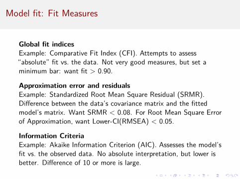
Global fit indicesExample: Comparative Fit Index (CFI). Attempts to assess“absolute” fit vs. the data. Not very good measures, but set aminimum bar: want fit > 0.90.
Approximation error and residualsExample: Standardized Root Mean Square Residual (SRMR).Difference between the data’s covariance matrix and the fittedmodel’s matrix. Want SRMR < 0.08. For Root Mean Square Errorof Approximation, want Lower-CI(RMSEA) < 0.05.
Information CriteriaExample: Akaike Information Criterion (AIC). Assesses the model’sfit vs. the observed data. No absolute interpretation, but lower isbetter. Difference of 10 or more is large.

R code to fit the 3-factor model
It is very simple to define and fit a CFA in R!
library(lavaan)
piesModel3 <- " General =~ i1 + i2 + i3Feature =~ i4 + i5 + i6 + i7Image =~ i8 + i9 + i10 + i11 "
pies.fit3 <- cfa(piesModel3, data=pies.data)
summary(pies.fit3, fit.measures=TRUE)
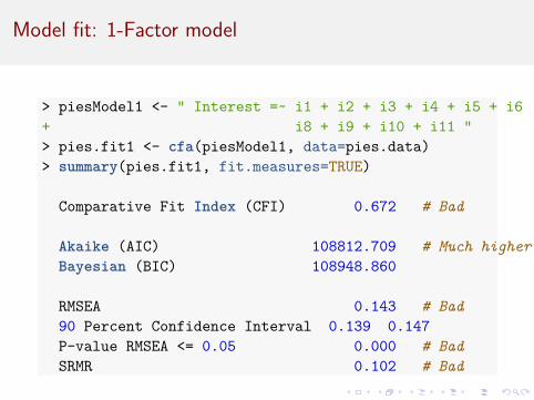
Model fit: 1-Factor model
> piesModel1 <- " Interest =~ i1 + i2 + i3 + i4 + i5 + i6 + i7 ++ i8 + i9 + i10 + i11 "> pies.fit1 <- cfa(piesModel1, data=pies.data)> summary(pies.fit1, fit.measures=TRUE)
Comparative Fit Index (CFI) 0.672 # Bad
Akaike (AIC) 108812.709 # Much higherBayesian (BIC) 108948.860
RMSEA 0.143 # Bad90 Percent Confidence Interval 0.139 0.147P-value RMSEA <= 0.05 0.000 # BadSRMR 0.102 # Bad

Model fit: 3-Factor model
> piesModel3 <- " General =~ i1 + i2 + i3+ Feature =~ i4 + i5 + i6 + i7+ Image =~ i8 + i9 + i10 + i11 "> pies.fit3 <- cfa(piesModel3, data=pies.data)> summary(pies.fit3, fit.measures=TRUE)
Comparative Fit Index (CFI) 0.975 # Excellent
Akaike (AIC) 105821.776 # Much lowerBayesian (BIC) 105976.494
RMSEA 0.041 # Excellent90 Percent Confidence Interval 0.036 0.045P-value RMSEA <= 0.05 1.000 # GoodSRMR 0.030 # Excellent
The 3-factor model is a much better fit to these data!

Model Paths
Latent Variables Estimate Std.Err Z-value P(>|z|)General =~
i1 1.000i2 0.948 0.042 22.415 0.000i3 1.305 0.052 25.268 0.000
Feature =~i4 1.000i5 1.168 0.037 31.168 0.000i6 0.822 0.033 25.211 0.000i7 1.119 0.036 31.022 0.000
Image =~i8 1.000i9 0.963 0.028 34.657 0.000i10 0.908 0.027 33.146 0.000i11 0.850 0.027 31.786 0.000

Visualize it
0.200.22
0.23
0.82 0.850.910.95 0.961.00 1.00 1.001.121.171.31
i1 i2 i3 i4 i5 i6 i7 i8 i9 i10 i11
Gnr Ftr Img

A few other points on CFA
Fixing pathsTo make a model identifiable, one path must be fixed between afactor and a variable. This makes paths interpretable relative tothat variable. Standardizing predictors is important so they’recomparable!
Modeling Factor CorrelationsYou might specify some factor correlations as low (e.g., 0.10) orhigh (e.g., 0.50). This is easy to do in R; differs in other packages.
Hierarchical ModelsYou can model higher-order factors, such as overall “productinterest”. CFA allows latent variables associated with other latentvariables . . . easy, but too complex for today! (See Chapter 10 inChapman & Feit for an example.)
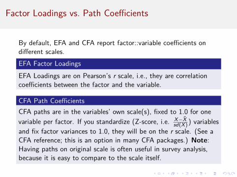
Factor Loadings vs. Path Coefficients
By default, EFA and CFA report factor::variable coefficients ondifferent scales.EFA Factor LoadingsEFA Loadings are on Pearson’s r scale, i.e., they are correlationcoefficients between the factor and the variable.
CFA Path CoefficientsCFA paths are in the variables’ own scale(s), fixed to 1.0 for onevariable per factor. If you standardize (Z-score, i.e. X−X̄
sd(X)) variablesand fix factor variances to 1.0, they will be on the r scale. (See aCFA reference; this is an option in many CFA packages.) Note:Having paths on original scale is often useful in survey analysis,because it is easy to compare to the scale itself.

Finally

The Main Points
1 If you use scales with multiple items, check them with EFA &CFA! Don’t just assume that your scales are correct, or thatitems load where you expect.
2 If you have multiple item scores – such as items that add up toa “satisfaction” score – consider using factor scores instead.
3 If you propose a complex model, prove with CFA that it’sbetter than alternatives.
4 This area has a lot of jargon but is not intrinsically difficult . . .and is much better than ignoring it and hoping for the best!SPSS, R, SAS, and Stata all have excellent factor analysistools.

Workflow for scale development
1 Identify factors of possible interest2 Write many items for those factors and field a survey3 Use EFA to identify whether the factors hold up, and which
items load on them4 Repeat 1-3 until you believe you have reliable factors and good
items5 Use CFA to demonstrate that the factors and items hold up in
a new sample
Example: PIES scale development paper, Chapman et al, 2009

Learning more: Books
1 Chapman & Feit (2015), R for Marketing Research andAnalytics. Chapters 8 and 10 present EFA and CFA inmarketing contexts, with detailed R code.
2 Pett, Lackey, & Sullivan (2003), Making Sense of FactorAnalysis. A practical guide to EFA with emphasis on(healthcare) survey development.
3 Brown (2015), Confirmatory Factor Analysis for AppliedResearch. An excellent & practical text on CFA for the socialsciences.
4 Kline (2015), Principles and Practice of Structural EquationModeling. The definitive guide for social science usage of CFAand SEM.
5 DeVellis (2011), Scale Development. A very practical andreadable guide to building good survey scales.
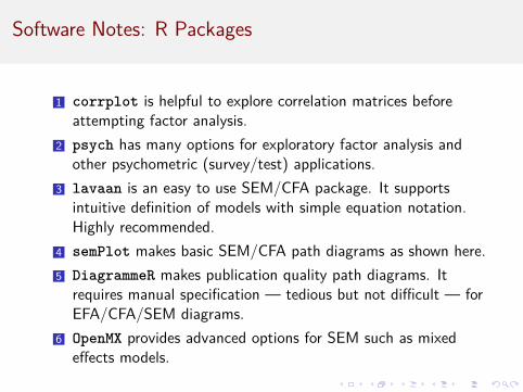
Software Notes: R Packages
1 corrplot is helpful to explore correlation matrices beforeattempting factor analysis.
2 psych has many options for exploratory factor analysis andother psychometric (survey/test) applications.
3 lavaan is an easy to use SEM/CFA package. It supportsintuitive definition of models with simple equation notation.Highly recommended.
4 semPlot makes basic SEM/CFA path diagrams as shown here.5 DiagrammeR makes publication quality path diagrams. It
requires manual specification — tedious but not difficult — forEFA/CFA/SEM diagrams.
6 OpenMX provides advanced options for SEM such as mixedeffects models.
