introduction to farm management - k.k.wagh n/3.farm management-i.pdf · introduction to farm...
TRANSCRIPT
Fdeveand diffetheirresouecon
Treaso
i) Faimpr
ii) Tare s
iii) Tpolit
iv) T
Ffarmcapitfarmsatisbetwand respe
Tskilldefin
A. D
Funde
INTRODUCTION TO FARM MANAGEMENT
arm business management has assumed greater importance not only in loped and commercial agriculture all round the world but also in developing subsistence type of agriculture. A farm manager must not only understand rent methods of agricultural production, but also he must be concerned with costs and returns. He must know how to allocate scarce productive rces on the farm business to meet his goals and at the same time react to
omic forces that arise from both within and outside the farm.
he need for managing an individual farm arises due to the following ns:
rmers have the twin objectives, viz., maximization of farm profit and ovement of standard of living of their families.
he means available to achieve the objectives, i.e., the factors of production, carce in supply.
he farm profit is influenced by biological, technological, social, economic, ical and institutional factors.
he resources or factors of production can be put to alternative uses.
arm management is concerned with resource allocation. On one hand, a er has a set of farm resources such as land, labour, farm buildings, working al, farm equipments, etc. that are relatively scarce. On the other hand, the er has a set of goals or objectives to achieve may be maximum family faction through increasing net farm income and employment generation. In een these two ends, the farmer himself is with a specific degree of ability awareness. This gap is bridged by taking a series of rational decisions in ct of farm resources having alternative uses and opportunities.
he study of farm management would be useful to impart knowledge and for optimizing the resource use and maximizing the profit. The following itions would throw light on the meaning of farm management:
EFINITIONS
arm means a piece of land where crop and livestock enterprises are taken up r a common management and has specific boundaries. All farm management
102
economists can be categorized into three groups on the basis of whether they consider farm management as an art, science or business.
The first group of farm management economists comprising of Andrew Boss, H.C.Taylor and L.C. Gray viewed farm management as “an art of organization and operation of the farm successfully as measured by the test of profitableness”.
The second group comprising of G.F. Warner and J.N. Effersen considered farm management “as a science of organization and operation of the farm enterprises for the purpose of securing the maximum profit on a continuous basis”.
The third group of economists like L.A. Moorehouse and W.J. Spillman defined farm management “as a study of the business phase of farming”.
The most acceptable definition of farm management is given below:
Farm Management is a science that deals with the organization and operation of a farm as a firm from the point of view of continuous maximum profit consistent with the family welfare of the farmer. Thus, in an environment where a farmer desires to achieve objectives like profit maximization and improvement of family standard of living with a limited stock of factors of production which can be put to alternative uses, farm management in an essential tool.
B. FARM MANAGEMENT DECISIONS
Farmers must be able to take appropriate decisions at appropriate time. Incorrect judgement and decisions would result in the failure of execution of farm plan and in turn economic loss. The farm management decisions can be broadly categorized into two ways.
i) The first method of classifications is according to the following criteria: a) Importance, b) Frequency, c) Imminence, d) Revocability and e) Alternatives available. Each of the above criteria is discussed briefly.
a) Importance: Farm management decisions vary as to the degree of importance measured generally through the magnitude of profit or loss involved. For example, a decision to engage in poultry is relatively more important than a decision regarding the type and location of poultry shed.
b) Frequency: Many decisions assume importance on the farm because of their high frequency and repetitive nature. The decision about what and how much to
103
feed to the dairy animals is made more frequently than that regarding the method or time of harvesting of paddy.
c) Imminence: It refers to the penalty or cost of waiting with respect to different decisions on the farm. Experience shows that while it pays to act quite promptly in some cases, postponement is necessary in other cases till the required complete information becomes available. For example, the decision to harvest paddy is much more imminent than a decision about buying a tractor.
d) Revocability: Some decisions can be altered at a much lower cost as compared to others. For example, it is relatively easier to replace paddy with groundnut, which perhaps becomes more profitable, than to convert a mango orchard into a sugarcane plantation.
e) Alternatives available: The number of alternatives can also be used for classifying farm management decisions. The decisions become more complicated as the number of alternatives increase. For example, threshing of paddy can be done manually or with thresher.
Classification of decisions based on the above criteria is not mutually exclusive and is changing from individual to individual and from place to place for the same individual.
ii) The second method classifies farm management decisions into: a) what to produce? b) when to produce? c) how much to produce? and d) how to produce?
The farm manager should choose the enterprises based on availability of resources on the farms and expected profitability of the enterprise. This is studied through product-product relationship. Once the farmer decides on what to produce, he must also decide on when to produce, as most of the agricultural commodities are season bound in nature. Then, he should decide how much of each enterprise to produce, since the supply of agricultural inputs is limited. This can be studied through factor-product relationship. In order to minimize the cost of production, i.e., decisions relating to how to produce, factor-factor relationship has to be studied. The farm manager should also take marketing decisions like a) what to buy? b) when to buy? c) how much to buy? d) how to buy? e) what to sell? f) when to sell? g) how much to sell? and h) how to sell?
iii) Factors Influencing Farm Management Decisions: Farm management decisions continuously undergo a change overtime because of the changing environment around the farm, farmer and his family. The factors which influence the decision making process are:
a) Economic factors like prices of factors and products.
104
b) Biological characteristics of plants and animals.
c) Technological factors like technological advancements in the field of agriculture and suitability of different varieties and farm practices to varied agro - climatic conditions.
d) Institutional factors like availability of infrastructural facilities which include storage, processing, grading, transport, marketing of inputs and outputs, etc, government policies on farm practices, input subsides, taxes, export and import, marketing, procurement of produces and so on.
e) Personal factors like customs, attitude, awareness, personal capabilities and so on.
One or more changes of the above categories in the environment around the farmer may cause imperfections in decision-making. The process of decision-making, therefore, has to be dynamic so as to adjust in such changes.
iv) Decision Making Process
Every farmer has to make decisions about his farm organization and operation from time to time. Decisions on the farms are often made by the following three methods:
a) Traditional method: In this method, the decision is influenced by traditions in the family or region or community.
b) Technical method: In this method, the decisions require the use of technical knowledge. For example, a decision is to be made about the quantity of nitrogen requirement to obtain maximum yield of paddy.
c) Economic method: All the problems are considered in relation to the expected costs and returns. This method is undoubtedly the most useful of all the methods for taking a decision on a farm.
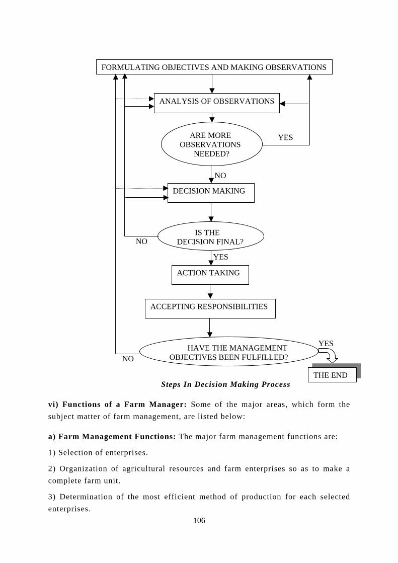
v) Steps in Decision Making
The steps in decision - making can also be shown schematically through a flow chart. The important steps involved in the decision-making process are formulating objectives and making observations, analyses of observations, decision-making, action taking or execution of the decisions and accepting the responsibilities. The evaluation and monitoring should be done at each and every stage of the decision making process.
105
vi) Functionsubject matte
a) Farm Man
1) Selection o
2) Organizaticomplete farm
3) Determinaenterprises.
FORMULATING OBJECTIVES AND MAKING OBSERVATIONS
S
S
NO
Steps In Decision Making Process
ANALYSIS OF OBSERVATIONS
ARE MORE OBSERVATIONS NEEDED?
DECISION MAKING
ACTION TAKING
ACCEPTING RESPONSIBILITIES
IS THE DECISION FINAL?
HAVE THE MANAGEMENT OBJECTIVES BEEN FULFILLED?
s of a Farm Manager: Some of the major areas, whicr of farm management, are listed below:
agement Functions: The major farm management functio
f enterprises.
on of agricultural resources and farm enterprises so as unit.
tion of the most efficient method of production for eac
106
THE END
YE
YES
h
n
t
h
YE
NO
NO
form the
s are:
o make a
selected
4) Management of capital and financing the farm business.
5) Maintenance of farm records and accounts and determination of various efficiency parameters.
6) Efficient marketing of farm products and purchasing of input supplies.
7) Adjustments against time and uncertainty elements on farm production and purchasing of input supplies.
8) Evaluation of agricultural policies of the government.
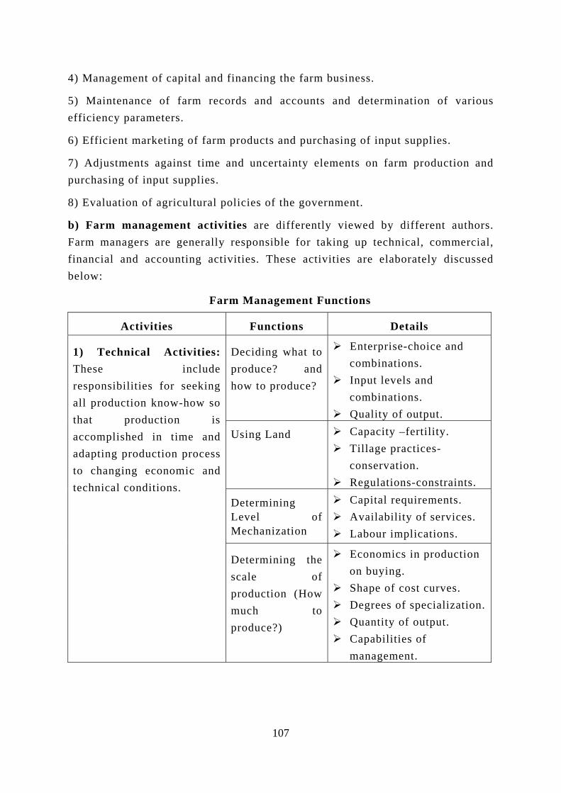
b) Farm management activities are differently viewed by different authors. Farm managers are generally responsible for taking up technical, commercial, financial and accounting activities. These activities are elaborately discussed below:
Farm Management Functions
Activities Functions Details
Dproduce?
eciding what to and
how to produce?
Enterprise-choice and combinations. Input levels and
combinations. Quality of output.
Using Land Capacity –fertility. Tillage practices-
conservation. Regulations-constraints.
Determining Level of Mechanization
Capital requirements. Availability of services. Labour implications.
1) Technical Activities: These include responsibilities for seeking all production know-how so that production is accomplished in time and adapting production process to changing economic and technical conditions.
Determining the scale of production (How much to produce?)
Economics in production on buying. Shape of cost curves. Degrees of specialization. Quantity of output. Capabilities of
management.
107
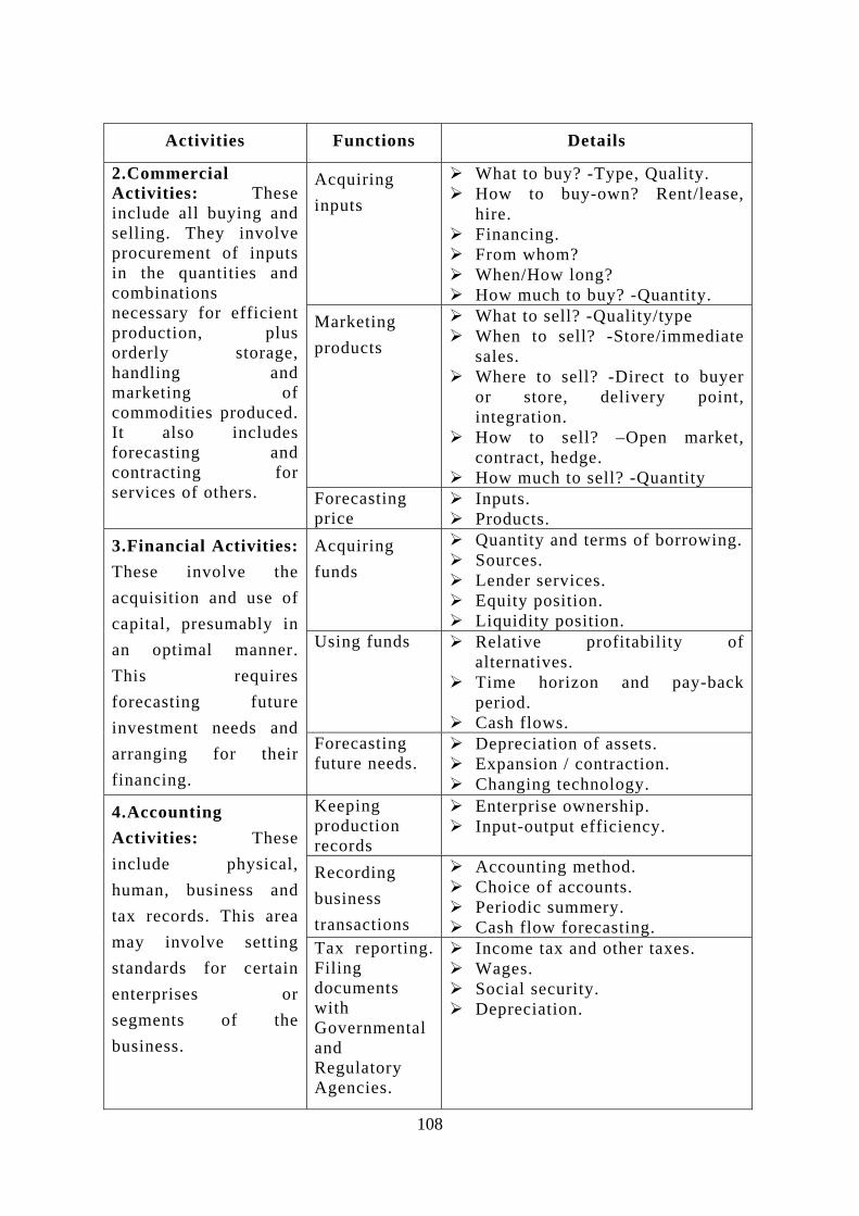
Activities Functions Details
Acquiring inputs
What to buy? -Type, Quality. How to buy-own? Rent/lease,
hire. Financing. From whom? When/How long? How much to buy? -Quantity.
Markeproduc
ting ts
What to sell? -Quality/type When to sell? -Store/immediate
sales. Where to sell? -Direct to buyer
or store, delivery point, integration. How to sell? –Open market,
contract, hedge. How much to sell? -Quantity
2.Commercial Activities: These include all buying and selling. They involve procurement of inputs in the quantities and combinations necessary for efficient production, plus orderly storage, handling and marketing of commodities produced. It also includes forecasting and contracting for services of others. Forecasting
price Inputs. Products.
Acquiring nds fu
Quantity and terms of borrowing. Sources. Lender services. Equity position. Liquidity position.
Using funds Relative profitability of alternatives. Time horizon and pay-back
period. Cash flows.
3.Financial Activities: These involve the acquisition and use of capital, presumably in an optimal manner. This requires forecasting future investment needs and arranging for their financing.
Forecasting future needs.
Depreciation of assets. Expansion / contraction. Changing technology.
Keeping production
ds recor
Enterprise ownership. Input-output efficiency.
Recobusiness
rding
transactions
Accounting method. Choice of accounts. Periodic summery. Cash flow forecasting.
4.Accounting Activities: These include physical, human, business and tax records. This area may involve setting standards for certain enterprises or segments of the business.
Tax reporting. Filing documents with Governmental and Regulatory Agencies.
Income tax and other taxes. Wages. Social security. Depreciation.
108
c) The third classification of farm management functions indicates that the farm management decisions or functions can be categorized into production, administration and marketing functions as depicted in the chart.
1) Production and Organization Decisions: The farm manager has to take vital decisions on production of enterprises and organization of his business. His decisions centre on what to produce and how to produce. Such decisions can be further classified into i) strategic and ii) operational decisions.
i. Strategic Management Decisions: These are the management decisions, which involve heavy investment and have long lasting effect. These decisions give shape to overall organization of the business.
a) Deciding the best size of the farm: The size of farm depends upon type of farm business, irrigation potential, level of mechanization, intensity of usage of land and managerial ability of the farmer. The economic efficiency of each crop/or live stock enterprise and their combinations, when they are operated on different scales, are considered to decide upon the optimum size of the holding.
b) Decisions on farm labour and machinery programmes: Deciding the most profitable combination of the factors to be used in producing a commodity is one of the important farm management decisions. What combination of farm labour and machinery should be adopted to get maximum returns? Would it be profitable to vary labour or land to better utilize a given set of machinery? These decisions are to be taken so as to reduce the cost of production.
c) Decisions on construction of buildings: Decisions on size and type of buildings involve heavy investment, which become fixed resource for the business. Type of buildings, for the present pattern and level of production depends upon the kind and level of crops or livestock produced.
d) Decisions regarding irrigation, conservation and reclamation programmes: As improvements of alkalinity, salinity and other soil defects require heavy investments, soil conservation and reclamation programmes often have to be spread over years. The choice of most economical method or a combination of methods of reclamation has to be made from among mulching, contouring, bunding, terracing and application of soil amendments, laying down of proper drainage and so on. Decision on irrigation programme is also very crucial because it involves heavy investment and it gives a flow service over long period of time and also improves the productivity of other related inputs.
109
PRODUCTION
AND
ORGANIZATION
PROBLEM
DECISIONS
ADMINISTRATIVE
PROBLEM
DECISIONS
MARKETING PROBLEM DECISIONS
FARM PROBLEMS REQUIRING DECISIONS OF THE FARMER
Farm Managemen
110
A. Strategic Decisions: (These involveheavy investment and have long lastingeffects) 1. Size of the Farm 2. Machinery and Livestock
Progranmmes 3. Construction of Building 4. Irrigation, Conservation and
Reclamation Programme. B. Operational Decisions: (morefrequent and involve relatively smallinvestments) 1. What to Produce? -Selection of
Enterprises 2. How much to Produce? - Enterprise
Mix and Production Process 3. How to Produce? – Selection of
Least Cost Method. 4. When to Produce? - Timing of
Production.
1. Financing the Farm Business: a) Optimum Utilization of Funds
b) Acquisition of Funds-Proper Agency and Time
2. Supervision of Work – Operational Timing 3. Accounting and Book Keeping 4. Adjustment of Farming Business to
Government Programmes and Policies
5. Production for Home Consumption and the Market.
t De
1.Buying a) What to buy? b) When to buy? c) From whom to buy? d) How to buy? e) How much to buy? 2.Selling a) What to sell? b) When to sell? c) To whom to sell? d) How to sell? e) How much to sell?
cisions
2. Operational Management Decisions: Operational management decisions are continuously made to carry out the day-to-day operations of the farm business. The investment involved in such decisions is relatively small and hence, the impact of such decisions is short-lived. These decisions are generally: i) what to produce? ii) how much to produce? how to produce? and when to produce? A brief discussion is made on these decisions below:
i) What to produce? (Selection of enterprises): The objective of the farm business, i.e., maximization of returns, could be achieved through the best combination of different enterprises. The relative profitability of these enterprises will be useful to determine what to produce and what not to produce.
ii) How much to produce? (Enterprise mix): This decision has two aspects: Enterprise mix and resource use.
a) Enterprise Mix: Combination of crop and livestock enterprises will depend upon the level of resources available, fertility of the soil, prices of factors and products in addition to the existence of complementary and supplementary relationship. Principle of substitution is used to decide the level of each enterprise, i.e., the scarce farm resources are first used for the most profitable enterprise and then the next best profitable enterprise is considered for inclusion. However, apart from profitability of each enterprise, factors like labour availability for each enterprise, size of land holding, use of by-products, maintenance of soil fertility, relative risks, distribution of incomes over time and efficiency in the use of machine power and building are considered to decide the level of each enterprise.
b) Resource Use: The best combination and optimum level of inputs can be determined based on the substitution principle and these have to be decided for minimizing the cost of production and maximization of returns.
iii) How to produce? (Selection of least - cost / efficient method or practice): Decisions, here, are made on the best practice or combination of practices and methods, which involve the least cost. The choice making from among the various alternatives has become a management problem. Although the objective generally is to select the least cost combination of inputs methods, consideration has to be given on the availability of resources in required quality and quantity at right time.
iv) When to produce? (Timing of production): Since the agricultural production is season-bound, it’s timing has to be properly decided. However,
111
farmer faces difficulty in selecting season, i.e., normal, early or late, for a particular crop due to non-availability of inputs in time and as a result he could not fetch maximum price for the produce.
3. Administrative Decisions
Along with production and organization decision, the former has to see that the work is done in a right way. Such administrative decisions are briefly discussed below:
i) Financing the farm business: While some farmers have their own sufficient funds, others may have to borrow. The problem is two fold, viz., a) utilization of funds within the farm business, and b) acquisition of funds, i.e., proper agency, time, type, and terms of credit. Cash flow analysis would be used to decide the timing and quantum of credit required.
ii) Supervision of work: The farm manager has to ensure that each job is scrupulously done as planned.
iii) Accounting and book keeping: Collection, analysis and evaluation of data have to be done in order to assess the performance of the farm at any point of time. Here decision is to be made on the kinds of farm records, time allocation and money to be spent on this activity.
iv) Adjustments to government programmes and policies: Government programmes and policies on food zones, restriction on product movements, price support policy, input subsidy, etc. influence farm production and marketing. The farmer has to decide on the level of production and resource-use with the maximum economic efficiency at the farm level consistent with the government policies concerned.
4. Marketing Decisions
A farm manager has to buy various farm inputs and sell out the produces in which he has to take rational decisions. While purchasing inputs he has to consider the following aspects: a) what to buy? b) when to buy? c) from whom to buy? d) how to buy? and e) how much to buy? Similarly, in selling out the farm produces he has to carefully ponder over the following points in order to maximize his farm income: a) what to sell? b) when to sell? c) to whom to sell? d) how to sell? and e) how much to sell?
vii) Relationship between Farm Management and Other Sciences
Farm management is an integral part of agricultural production economics. Farm management is an intra farm science whereas agricultural production economics is an inter farm or inter region science. The distinction sometimes
112
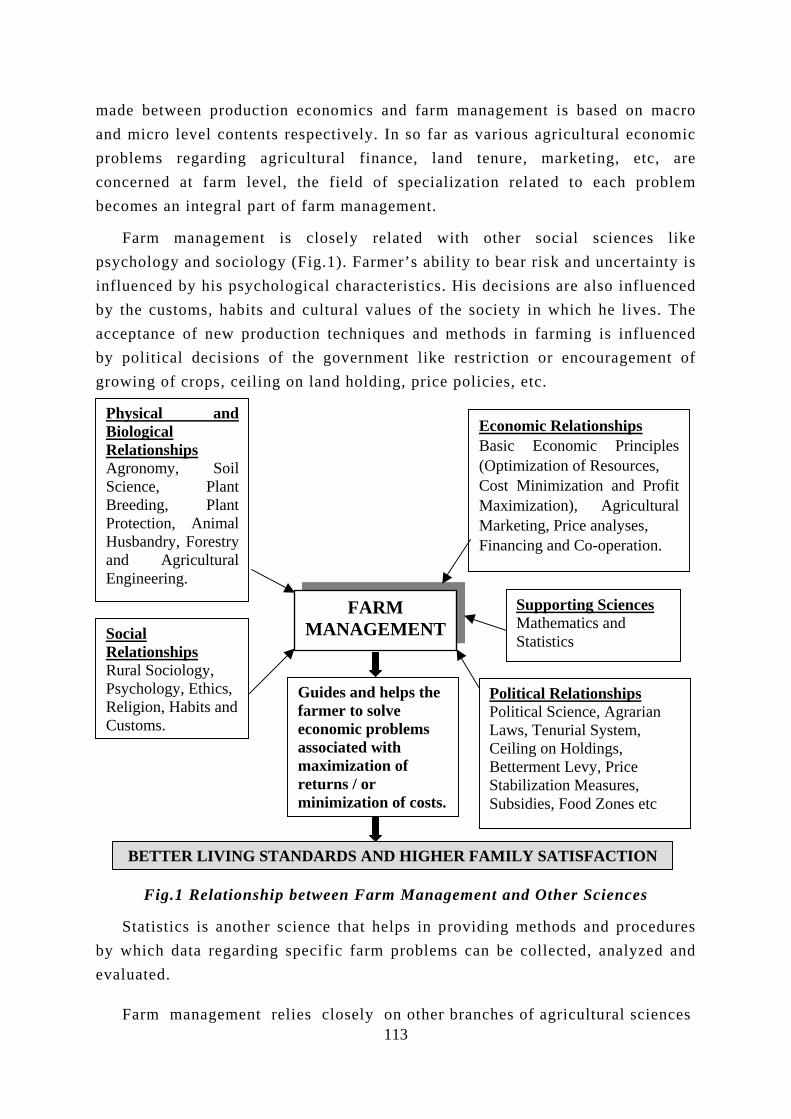
made between production economics and farm management is based on macro and micro level contents respectively. In so far as various agricultural economic problems regarding agricultural finance, land tenure, marketing, etc, are concerned at farm level, the field of specialization related to each problem becomes an integral part of farm management.
Farm management is closely related with other social sciences like psychology and sociology (Fig.1). Farmer’s ability to bear risk and uncertainty is influenced by his psychological characteristics. His decisions are also influenced by the customs, habits and cultural values of the society in which he lives. The acceptance of new production techniques and methods in farming is influenced by political decisions of the government like restriction or encouragement of growing of crops, ceiling on land holding, price policies, etc.
FARM MANAGEMENT
Physical andBiological Relationships Agronomy, SoilScience, PlantBreeding, PlantProtection, AnimalHusbandry, Forestryand AgriculturalEngineering.
Economic Relationships Basic Economic Principles(Optimization of Resources, Cost Minimization and ProfitMaximization), AgriculturalMarketing, Price analyses, Financing and Co-operation.
Supporting Sciences Mathematics and Statistics
Political Relationships Political Science, Agrarian Laws, Tenurial System,
be
Social Relationships Rural Sociology, Psychology, Ethics,Religion, Habits and Customs.
Ceiling on Holdings, Betterment Levy, Price Stabilization Measures, Subsidies, Food Zones etc
Fig.1 Relationship
Statistics is another scy which data regarding svaluated.
Farm management rel
Guides and helps the farmer to solve economic problems associated with maximization of returns / or minimization of costs.
N
BETTER LIVING STANDARDS AND HIGHER FAMILY SATISFACTIO
between Farm Management and Other Sciences
ience that helps in providing methods and procedures pecific farm problems can be collected, analyzed and
113ies closely on other branches of agricultural sciences
such as agronomy, soil science, plant protection studies, animal husbandry, agricultural engineering, forestry, etc. These physical and biological sciences are not directly concerned with economic efficiency. They provide input-output relationships in their respective areas in physical terms, i.e., they define production possibilities within which various choices can be made. It is the task of the farm management specialist and agricultural economist to determine how and to what extent the findings of these sciences should be used in farm business management.
viii) Characteristics of Farming as Business: Farming as a business has many distinguishing features from most of other industries in their management methods and practices. The major differences between farming and other industries are:
1) Agricultural production is biological is nature.
2) Agricultural production heavily depends on agro-climatic conditions.
3) Agricultural production is carried out mostly in small - sized holdings.
4) Frequent and speedy decisions are to be taken up in agricultural production. For instance, there is no time to consider the merits of paying more wages to drain the field when there is a sudden monsoon floods.
5) Agricultural prices and production usually move in opposite direction.
6) Lack of standardization of practices and products: By the use of machines and trained personnel, it is possible to produce large volume of products exactly the same in size, form and quality. Such standardization of practices and products is not possible in agriculture. Grading system for agricultural commodities is also very weak.
7) Slow turn -over: It takes long time to recover the investment.
8) Farm financing is more risky due to drought, pest and disease attack, yield variations, etc.
9) The proportion of fixed cost is more in agriculture and so adjustment and substitution of resources are more difficult.
10) Inelastic income demand for farm products: As income increases, the demand for agricultural products will increase in lesser proportion when compared with industrial goods.
11) Perishable and bulky nature of agricultural commodities cause storage, processing and transportation problems.
114
12) Lack of Knowledge: All farmers do not know the latest developments in agricultural technologies.
13) Agricultural markets are not regulated properly and there are too many middlemen in the agricultural marketing system, whereas in industry, the distribution channels are well defined and controlled by producers.
14) Agriculture is considered not only a means of livelihood but also a way of life to the farmers in all the under developed countries.
ix) Farm Management Problems under Indian Conditions
Farm management problems in India vary from place to place depending mostly on the degree of infrastructural development and the availability of resources. The following are some of the most common problems in the field of farm management:
1) Small size of farm business: The average size of operational holding in India was 1.55 ha in 1990-91. The holdings are fragmented, too. Unfavourable land-man ratio due to excessive family labour depending upon agriculture have weakened the financial position of the farmers and limited the scope for farm business expansion.
2) Farm as a household: In most parts of the country, farmers, especially dry land farmers, follow the traditional combinations of crops and methods of cultivation. Work habits are closely associated with food commodities consumed and living conditions. Farm has become the means of livelihood of farmers and hence, subsistence farming is followed. Home management, thus, heavily influences and gets influenced by farm management decisions.
3) Inadequate capital: The new technology demands costlier inputs such as fertilizer, plant protection measures, irrigation and high yielding variety seeds as well as investment on power and machinery. But perpetual debt and low marketable surplus prevent the farmers from adopting new technologies. 4) Under employment: Unemployment results from 1) small size of farm, 2) large supply of family labour, 3) seasonal nature of production and 4) lack of subsidiary or supporting rural industries. It reduces efficiency and productivity of rural manpower. 5) Slow adoption innovations: Small farmers are usually conservative and sometimes skeptical of new techniques and methods. However, once they try a new idea and find it effective, they are eager to adopt that. The rate of adoption, however, depends on farmer’s willingness and his ability to use the new information.
115

6) Inadequacy of input supplies: Farmers may be willing to introduce change, yet they may face the difficulty in obtaining the required inputs of proper quality, in sufficient quantity and on time in order to sustain the introduced changes.
7) Lack of managerial skill: Due to lack of managerial skill among small farmers, adoption of new techniques and use of costly inputs could not be followed up by them.
8) Lack of infrastructural facilities: Infrastructural facilities such as marketing, transport, and communication are either inadequate or inefficient and this results in the shortage of capital and quality inputs and non-availability of inputs in time. Chapter 8: Questions for Review. 1. Fill up the blanks i) Farmers have the objectives like and improvement of their family living standards. ii) Farm management is the study of phase of farming. iii) Management decisions, which involve heavy investment and have long lasting effect are called . iv) Perishable and bulky nature of agricultural commodities cause storage, processing and problems. v) Farm management is an intra farm science while, agricultural production economics is science. 2. i) Define Farm Management as a science. ii) Define agricultural production economics. 3. Write short notes i) Different methods of farm management decisions. ii) Factors influencing decision-making process. iii) Farm management goals. iv) Strategic decisions. 4. Answer the following: i) Explain the functions of farm manager. ii) What are the steps involved in the decision making process? iii) Explain the scope of farm management. iv) Explain how farm management is related to different disciplines. v) Explain the farm management problems faced by the Indian farmers. vi) Explain the characteristics of farming as a business. vii) Explain the different operational management decisions. viii) Explain the marketing decisions to be taken up by the farm manager.
116
BASIC CONCEPTS OF FARM MANAGEMENT
The basic concepts that are frequently used in farm management are discussed below:
i) Farm-Firm: Farm means a piece of land where crop and livestock enterprises are taken up under a common management. A farm is a firm which combines resources in the production of agricultural products on the lines of a business firm, i.e., with the objective of profit maximization.
ii) Resources or Inputs or Factors of Production: Resources are those which get consumed or transformed into products in the process of production. Services of resources are also used up in the production process. All agricultural resources can be classified into two types. They are i) fixed resources and ii) variable resources.
a) Fixed resources: Level of some resources like buildings, machinery, etc. is fixed over a production-planning period irrespective of the level of enterprises taken up. These are called fixed farm resources, E.g. Land, building, machineries, etc. The quantum of fixed resources does not change with the level of production. Some of the resources, which are fixed during a short period, may become variable during a long term.
b) Variable resources: Some resources like seed, fertilizer, labour, etc vary with the level of output. These are variable resources.
Resources can also be classified into stock and flow resources as detailed below:
a) Stock resources: They are resources which are used up entirely in the production process. Fertilizer, seed, feed, etc., are such resources that can be stored up for using at later period.
b) Flow resources: Contrary to stock resources, there are factors of production which give only flow of services in the production process. Hence, they are called the flow resources. If the services of this category of resources are not utilized, they go waste, as they cannot be stored up for later use. For example, if the services of a farm building or machinery are not used in a particular day, they go waste, as they cannot be stored up for future use.
iii) Ways of Mobilizing Farm Resources: The different types of farm resources and ways of mobilizing them by a farm manager are discussed here.
117
a) Owning: Resources like land, machinery, implements, tools, work bullocks, etc, can be acquired by purchasing them. Farmers can own these resources due to the following reasons:
1) The resources are to be continuously or more frequently used throughout the year. The size of holding should be large enough to effectively use such assets.
2) If the farmer could not engage work bullocks, tractors/power tillers, power sprayers, bullock cart and so on in his own farm economically, adequate demand should be there for hiring out these resources.
3) The farmer should have either adequate owned funds or borrowed funds to acquire these resources.
Owning of resources would be convenient to the farmer especially during peak season so as to carry out the farm operation in time. However, during lean season, it may be uneconomical to maintain owned resources. E,g. Bullocks, thresher, etc. Hiring would be cheaper than owning the resource especially, when the size of holding is too small.
b) Leasing: The immovable resources like land and buildings can be acquired by leasing. Rent has to be paid based on the terms agreed by the lessees (tenants) to the owner of such resources. The land owner may lease-out his lands to land less agricultural labourers or to farmers who are capable of cultivating larger area. The land owner leases out due to 1) his absenteeism at the village where his land is located, 2) inefficiency in running farm and 3) running of other more profitable enterprise in the same village. Sometimes, the widows and invalids may lease out due to their physical inability. Leasing-in helps lessees (tenants) to augment their farm returns. However, leasing-out becomes complicated due to improper implementation of agrarian laws which are more favourable to tenants. The fertility status of the leased-out land is gradually deteriorating because the tenants do not apply organic manure and they do not properly maintain the farm assets out of the fear of eviction from the land by the owner. Therefore, the productivity of leased-out land is lesser than that of owned land. On the contrary, as the tenancy legislations are more favourable to tenants, some of them refuse to surrender their tenancy rights to the owners and hence, the owners are reluctant to lease out their lands.
c) Hiring: The farmer can acquire human labour and bullock power through hiring. The magnitude of employment of hired human labour and bullock power
118
depends upon: a) size of farm holding, b) number of family labourers available, c) availability of owned bullocks, d) resourcefulness of the farmer to replace labour with capital and e) diversification of crop activities practiced in the farm. Hiring of human labour and bullock power is also difficult and costly during peak season due to either costly human labour as a result of heavy demand for such labour or difficulty in carrying the operations with human labour in time. However, hiring of human labour and bullock power is more economical than that of hired machinery to small and marginal farms, especially in areas where the labour is cheaper.
d) Joint ownership: When the land, buildings and well are inherited by legal heirs, the land gets sub-divided and buildings and wells are jointly owned among them. Joint ownership is convenient and economical to those who have small and fragmented inherited land. However, disputes arise due to lack of understanding among joint owners in sharing the services and also in the maintenance of the jointly owned assets.
e) Custom Services: Farmers could acquire custom services of machineries like tractor, power tillers, threshers, power sprayers, etc. by paying custom hire charges. Hiring of custom services of machineries depends upon 1) size of farm holding, 2) availability of alternatives such as human labour and bullock power, 3) hire charges for human labour and bullock power, 4) custom hire charges, 5) time of operation (peak or lean season), 6) availability of time to carry out the farm operation and 7) quantum of work to be carried out. Custom services would be more economical for small and marginal farms as they cannot afford to buy or maintain costlier equipments and machineries.
iv) Product or Output: It is the result of the use of resources or services of resources. The resources get transformed into what is known as output. E.g. Paddy, groundnut, sugarcane, milk, etc.
v) Production: It is a process of transformation of resources or inputs like labour, seed, fertilizer, water, etc. into products like paddy, wheat etc.
vi) Transformation or Production Period: The time required for a resource to be completely transformed into a product is called transformation or production period. E.g. Paddy is harvested in 3½ to 6 months.
vii) Production Economics: Farm production economics is a field of specialization within the subject of agricultural economics. It is concerned with
119
choosing of available alternatives or their combinations in order to maximize the returns or to minimize the costs. Agricultural production economics is an applied field of science, wherein the principles of choice are applied to the use of land, labour, capital and management in farming. The subject matter of production economics explains the conditions under which the profit, output, etc. that can be maximized and the cost, use of physical inputs, etc. that can be minimized. The main objectives of production economics are:
a) to determine and define the conditions which provide for optimum use of resources; b) to determine the extent to which the current use of resources deviates from the optimum use; c) to analyze the factors which influence the existing production patterns and resources use; and d) to identify the means and methods for optimal use of resources.
The principles that help attain these objectives are the same on a micro as on a regional or national level. On micro level where intra-farm resource allocation and production pattern are involved, it is the subject matter of farm management. When choice principles involve a broader field on a macro-level, the subject is known as production economics. The economist who focuses his attention on individual farm cannot make rational recommendations unless he considers the aggregate or overall aspect of production. Similarly, government programmes and policies affect the decisions on the individual farms. Production economist, therefore, must be able to integrate both individual and aggregate aspects of agricultural resource use and levels and patterns of production.
viii) Production Function: Production function refers to input-output relationship in the production process. Production function is a technical and mathematical relationship describing the manner and extent to which a particular product depends upon the quantities of inputs or services of inputs used in the production process. It describes the rate at which resources are transformed into products. There are numerous input-output relationships in agriculture because the rates at which inputs are transformed into outputs will vary among soil types, animals, technologies, rainfall, etc. Any given input-output relationship specifies the quantities and qualities of resources needed to produce a particular product.
a) Types of Production Function: There are different types of production functions, viz., 1) continuous function and 2) discontinuous function.
1) Continuous function: The doses or levels of input and output can be split up into small units. E.g. Fertilizers or seed can be applied to a hectare of land in quantities ranging from a fraction of a kilogram upto hundreds of kilograms.
120
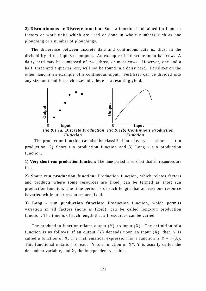
2) Discontinuous or Discrete function: Such a function is obtained for input or factors or work units which are used or done in whole numbers such as one ploughing or a number of ploughings.
The difference between discrete data and continuous data is, thus, in the divisibility of the inputs or outputs. An example of a discrete input is a cow. A dairy herd may be composed of two, three, or most cows. However, one and a half, three and a quarter, etc, will not be found in a dairy herd. Fertilizer on the other hand is an exampl of a continuous input. Fertilizer can be divided into any size unit and for ch si e unit, there is a resulting yield.
Out
put
Out
put
The prodproduction, 2function.
1) Very short fixed.
2) Short runand productsproduction fuis varied whil
3) Long - variation in function. The
The produfunction is acalled a funcThis functiondependent va
.
uc)run
p wncte o
runall tim
ctis fotional riab
.
tioSho
p
rodheionthe
p fae
onllo o
notle
.
n frt
rod
ure . r
rct
is
fuw
f Xat
, a
.ea
unc ru
uct
ctiosom
Thereso
oduorsof s
ncts: I. T
ion nd X
.e
tion
ion
n fe
timur
cti (nuc
ionf aheis , t
.z
0 Input 0 Input Fig.9.1 (a) Discrete Production Fig.9.1(b) Continuous Production
Function Function
n can also be classified into 1) very short run production function and 3) Long - run productionfunction: The time period is so short that all resources are
unction: Production function, which relates factors resources are fixed, can be termed as short run
e period is of such length that at least one resource ces are fixed.
on function: Production function, which permits one is fixed), can be called long-run production
h length that all resources can be varied.
relates output (Y), to input (X). The definition of a n output (Y) depends upon an input (X), then Y is
mathematical expression for a function is Y = f (X). read, “Y is a function of X”. Y is usually called the he independent variable.
121
b) Subscripts: Subscripts are useful when symbols are used. Consider, for example, the notation for the production function Y = f (X), where X is the amount of input and Y, the resulting amount of output. In this, there can be no confusion about identification of input or output because there is only one input and one output. When more than one input or output is included in a problem, subscripts can be used as a means of identification. For example, when output is a function of three inputs, the production function can be written Y = f (X1, X2, X3), where X1, X2 and X3 are distinct and different inputs. X1 may be seeds; X2 may denote labour and X3 may indicate fertilizer. If amounts are to be denoted, additional subscripts must be used. X11 is an amount of X1; X12 is a greater amount of X1; X21 is an amount of X2; X22 is a greater amount of X2; etc. Subscripts can also be used to identify outputs or any other variable. Thus, Y1, Y2 and Y3 can be distinct outputs and the amounts can be shown by adding
another subscript.
c) The “∆” (Delta) Notation: The change in any variable is denoted by “∆” (the Greek letter “delta”) placed before the variable. For example, the change in the variable X is denoted by ∆X. Production function is written as: Y = f (X1, X2, X3,..., Xn) where, Y is output and X1, ..., Xn are different inputs that are used in
the production of a product or output. The functional symbol “f” indicates the form of relationship that transforms inputs into output. For each combination of inputs, there will be a unique level of output. For example, Y may represent paddy yield, X1, quantity of seed, X2, quantity of fertilizer, X3, labour and so on.
The above notation for a production function does not specify which inputs are fixed and which are variable. For example, seed or fertilizers are variable inputs that are combined with fixed input such as acre of land. Symbolically, fixed inputs can be included in the notation for a production function by inserting a vertical line between the fixed and variable inputs. For example, Y = f (X1, X2, X3, ... Xn-1 | Xn) states that Xn is the fixed input while all other inputs are
variable.
d) Forms of Production Function: The technical functional relationship between resources/inputs and product can be expressed by a functional form, a few of which are given below:
n
1) Linear: The simplest form of linear production function is Y = a + bX with one variable input and Y = a + b1X1 + b2X2 + b3X3 + ... + bnXn with n variables.
Σ bi Xi . i = 1
Symbolically, Y= a + where, Y is output, a - constant, bi – unknown
122
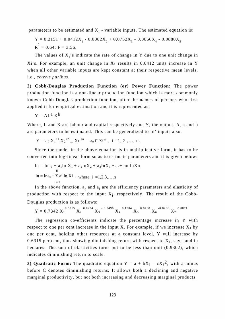
parameters to be estimated and Xi - variable inputs. The estimated equation is:
Y = 0.2151 + 0.0412X1 - 0.0002X2 + 0.0752X3 - 0.0066X4 - 0.0880X5
R2 = 0.64; F = 3.56.
The values of Xi’s indicate the rate of change in Y due to one unit change in
Xi’s. For example, an unit change in X1 results in 0.0412 units increase in Y when all other variable inputs are kept constant at their respective mean levels, i.e., ceteris paribus.
2) Cobb-Douglas Production Function (or) Power Function: The power production function is a non-linear production function which is more commonly known Cobb-Douglas production function, after the names of persons who first applied it for empirical estimation and it is represented as:
Y = ALa Kb
Where, L and K are labour and capital respectively and Y, the output. A, a and b are parameters to be estimated. This can be generalized to ‘n’ inputs also.
Y = a0 X1a1
X2a2
… Xnan = a0 Π Xia i
, i =1, 2 ,…, n.
Since the model in the above equation is in multiplicative form, it has to be converted into log-linear form so as to estimate parameters and it is given below:
n ln = lna0 + a1ln X1 + a2lnX2 + a3lnX3 +…+ an lnXn
ln = lna0 + Σ ai ln Xi , where, i =1,2,3,…,n i = 1
In the above function, a0 and ai are the efficiency parameters and elasticity of production with respect to the input Xi, respectively. The result of the Cobb-
Douglas production is as follows:
Y = 0.7342 X10.6315
X2 0.0234
X3 - 0.0496
X4 0.1904
X5 0.0760
X6 -0.0286
X7 0.0871
The regression co-efficients indicate the percentage increase in Y with respect to one per cent increase in the input X. For example, if we increase X1 by one per cent, holding other resources at a constant level, Y will increase by 0.6315 per cent, thus showing diminishing return with respect to X1, say, land in hectares. The sum of elasticities turns out to be less than unit (0.9302), which indicates diminishing return to scale.
3) Quadratic Form: The quadratic equation Y = a + bX1 – cX12, with a minus before C denotes diminishing returns. It allows both a declining and negative marginal productivity, but not both increasing and decreasing marginal products.
123

ix) Total Physical Product (TPP): TPP is the quantum of output (Y) produced by a given level of input (X).
x) Average Physical Product (APP): APP is the quantity of output produced per unit of input i.e., ratio of the total product to the quantity of input used in producing that amount of product.
xi) Marginal Physical Product (MPP): The term marginal refers to an additional unit. If we use ∆ (delta) to mean “change in “, then ∆Y and ∆X represent change in Y (output) and change in X (input) respectively. Marginal physical product, therefore, refers to the change in output, which results from applying an additional unit of input.
Change in Output ∆ Y Marginal Physical Product (MPP) = =
Change in Input ∆ X Chapter 9: Questions for Review: 1. Fill up the following blanks: i) The level of fixed resources will with the level of output. ii) In long run, no cost is . iii) Farm management is generally considered to fall in the field of economics. iv) In Cobb-Douglas production function, the regression co-efficient are the of production with respect to their respective inputs. v) Interest on operational expenses falls under resource. vi) In linear regression function, the regression co-efficients indicate . vii) In the very short run production function, all resources are .
Number of Units of Output Y APP = = Number of Units of Input X
2. Define the following: i) Farm. ii) Short run and long run. iii)Continuous and Discrete Production functions. iv) Stock and flow resources. v) Product and production period. 3. Write short notes: i) Production function. ii) Total, Average and Marginal Physical Products. iii)Fixed and variable resources. iv) Production economics and Farm management. 4. Answer the following: i) Explain the different types of production functions and indicate how they are useful in farm decision-making. ii)Explain the different ways of mobilizing various farm inputs and indicate their merits and demerits. iii)How leasing is different from custom hire service of a resource?
124
The objective of factor-product relationship is to determine the optimum quantity of the variable input that will be used in combination with fixed inputs in order to produce optimal level of output. Further questions such as, how much fertilizer to be applied per acre? how much irrigation to be given? and so on are all within the scope of factor – product relationship. There can be three types of input-output relationships in producing a commodity where one input is varied and the quantities of other inputs are fixed. The nature of relationships between a single input and a single output can either be of the one or a combination of types given below:
i) Constant Marginal Rate of Returns or Law of Constant Returns.
ii) Increasing Marginal Rate of Returns or Law of Increasing Returns.
iii) Decreasing Marginal Rate of Returns or Law of Decreasing Returns.
A. LAWS OF RETURNS
Let us consider the simplest case where one product is produced by varying the level of only one factor of production at a time.
Out
put (
Y)
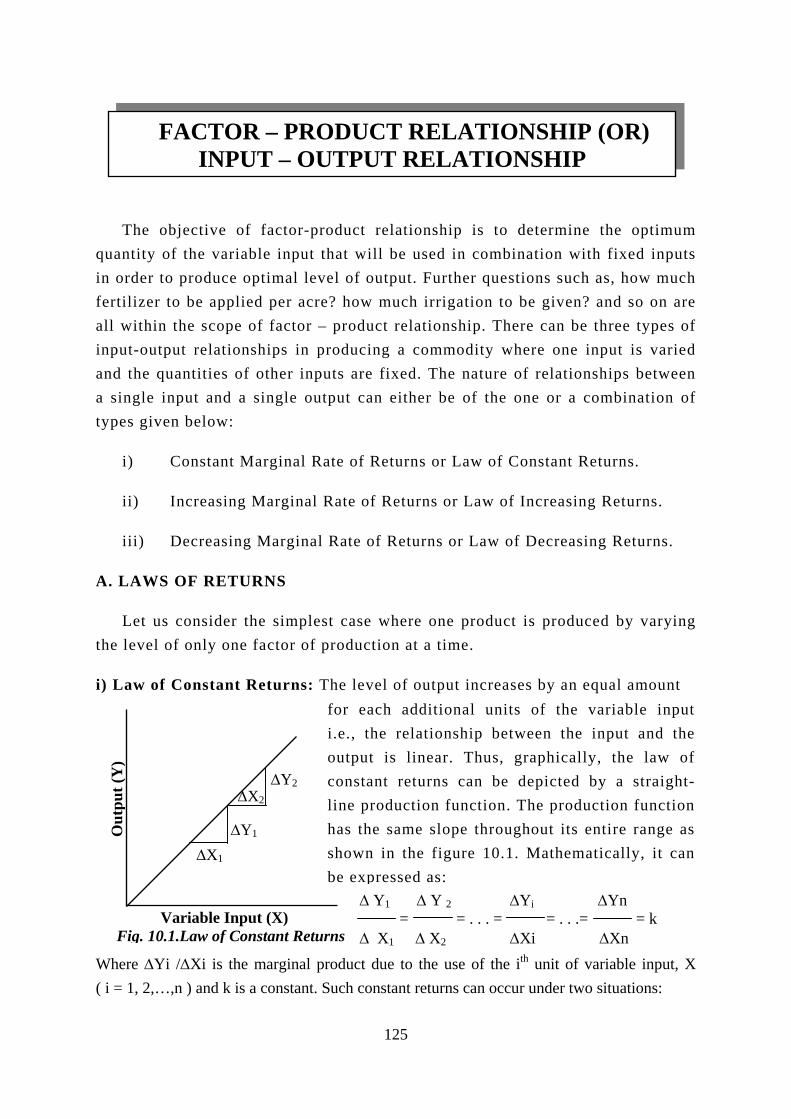
i) Law of Constant Returns:
∆ Y1 ∆ Y 2 ∆Yi ∆Yn = = . . . = = . . .= = k ∆ X1 ∆ X2 ∆Xi ∆Xn
W( i
Variable Input (X) Fig. 10.1.Law of Constant Returns
here ∆Yi /∆ = 1, 2,…,n )
∆X1
Xi is t and k
∆X2
∆Y1
he m is a c
∆Y2
FACTOR – PRODUCT RELATIONSHIP (OR) INPUT – OUTPUT RELATIONSHIP
arginal ponstant.
for each additional units of the variable inputi.e., the relationship between the input and theoutput is linear. Thus, graphically, the law ofconstant returns can be depicted by a straight-line production function. The production functionhas the same slope throughout its entire range asshown in the figure 10.1. Mathematically, it canbe expressed as:
The level of output increases by an equal amount
roduct due to the use of the ith unit of variable input, X Such constant returns can occur under two situations:
125
a) No resource is fixed and all the inputs are varied, increased or decreased together.
b) One or more factors of production may be fixed but they have surplus (unutilized) capacity. The constant returns may be explained with the data given below:
Table 10.1 Yield of Maize at Varying Levels of Nitrogen per Hectare
Variable Inputs
(Kg of N per ha)
∆Xi Output (quintals of
Maize per ha)
∆Yi
0 - 25 - -
25 25 26 1 0.04
50 25 27 1 0.04
75 25 28 1 0.04
100 25 29 1 0.04
The table (10.1) shows that every addition of 25 Kg of nitrogen ∆Xi causes exactly the same increase of one quintal in the yield of maize per ha (∆Yi) during the process of production.
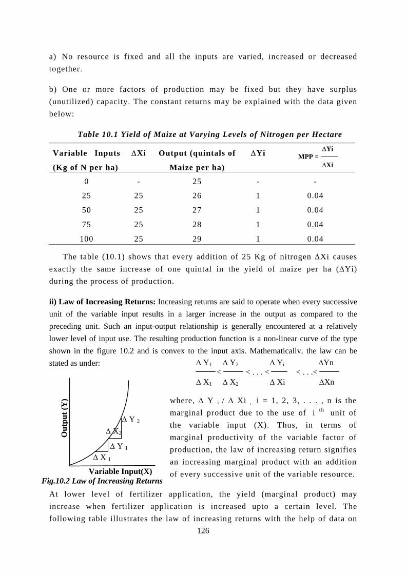
ii) Law of Increasing Returns: Increasing returns are said to operate when every successive unit of the variable input results in a larger increase in the output as compared to the preceding unit. Such an input-output relationship is generally encountered at a relatively lower level of input use. The resulting production function is a non-linear curve of the type shown in the figure 10.2 and is convex to e stated as under:
Out
put (
Y)
VariaFig.10.2 Law of Inc
where, ∆ Y i / ∆ Xi , .i = 1, 2, 3, . . . , n is themarginal product due to the use of .i th unit ofthe variable input (X). Thus, in terms ofmarginal productivity of the variable factor ofproduction, the law of increasing return signifies
At lower leveincrease when following table
∆ Y 1
2
an increasing marginal product with an addition
∆ X 1 blereal ofe ill
∆ Y 2
∆ XInput(X) sing Returns
of eve
f fertilizer applicartilizer applicationustrates the law of
the input axis. Mathematically, the law can b∆ Y1 ∆ Y2 ∆ Yi ∆Yn < < . . . < < . . .< ∆ X1 ∆ X2 ∆ Xi ∆Xn
ry successive unit of the va
tion, the yield (margina is increased upto a cerincreasing returns with the126
∆Yi MPP =
∆Xi
riable resource.
l product) may tain level. The help of data on
paddy yield at varying levels of nitrogen application. The example given in the table (10.2) indicates the response of paddy yield to increasing nitrogen
application at a very low level of the input–use. It may be observed that as the input is increased from 0 to 25 kgs per hectare, a dose of 5 kg at each step, the
Table 10.2 Yield of Paddy at Varying Levels of Nitrogen per Hectare Table 10.2 Yield of Paddy at Varying Levels of Nitrogen per Hectare
Variable Input (Kg of nitrogen per Ha) Variable Input (Kg of nitrogen per Ha)
∆ Xi ∆ Xi Output (Quintals of paddy per Ha) Output (Quintals of paddy per Ha)
∆ Y i∆ Y i
0 - 20.0 - - 5 5 21.0 1.00 0.20 10 5 22.5 1.50 0.30 15 5 24.5 2.00 0.40 20 5 27.0 2.50 0.50 25 5 29.7 2.70 0.54
yield increases by 1.0, 1.5, 2.0, 2.5 and 2.7 quintals per hectare. Thus, every successive dose of 5 Kgs of nitrogen results in more output of paddy signifying the operation of the law of increasing returns.
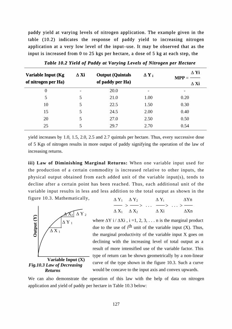
iii) Law of Diminishing Marginal Returns: When one variable input used for the production of a certain commodity is increased relative to other inputs, the physical output obtained from each added unit of the variable input(s), tends to decline after a certain point has been reached. Thus, each additional unit of the variable input results in less figure 10.3. Mathematically,
Out
put (
Y)
We can also demonstraapplication and yield of p
∆ Y 2
∆ X2∆ Y 1
∆ X 1
Variable Input (X) Fig.10.3 Law of Decreasing Returns
te the operation of this law with the help of daddy per hectare in Table 10.3 below:
127
∆ YiMPP =
∆ Xi
and less addition to the total output as shown in the
where ∆Y i / ∆Xi , i =1, 2, 3, . . . n is the marginal productdue to the use of ith unit of the variable input (X). Thus,the marginal productivity of the variable input X goes ondeclining with the increasing level of total output as aresult of more intensified use of the variable factor. Thistype of return can be shown geometrically by a non-linearcurve of the type shown in the figure 10.3. Such a curvewould be concave to the input axis and convex upwards.
∆ Y1 ∆ Y2 ∆ Yi ∆Yn > > . . . > . . . > ∆ X1 ∆ X2 ∆ Xi ∆Xn
ata on nitrogen
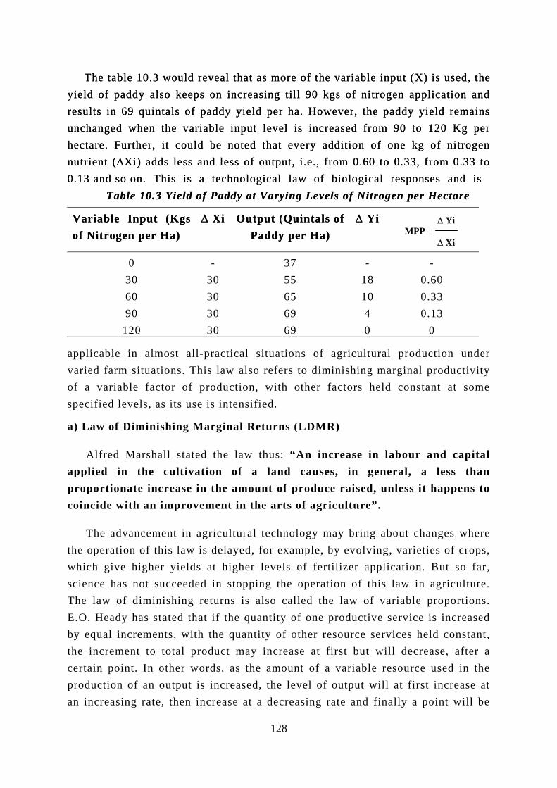
The table 10.3 would reveal that as more of the variable input (X) is used, the yield of paddy also keeps on increasing till 90 kgs of nitrogen application and results in 69 quintals of paddy yield per ha. However, the paddy yield remains unchanged when the variable input level is increased from 90 to 120 Kg per hectare. Further, it could be noted that every addition of one kg of nitrogen nutrient (∆Xi) adds less and less of output, i.e., from 0.60 to 0.33, from 0.33 to 0.13 and so on. This is a technological law of biological responses and is
The table 10.3 would reveal that as more of the variable input (X) is used, the yield of paddy also keeps on increasing till 90 kgs of nitrogen application and results in 69 quintals of paddy yield per ha. However, the paddy yield remains unchanged when the variable input level is increased from 90 to 120 Kg per hectare. Further, it could be noted that every addition of one kg of nitrogen nutrient (∆Xi) adds less and less of output, i.e., from 0.60 to 0.33, from 0.33 to 0.13 and so on. This is a technological law of biological responses and is
Table 10.3 Yield of Paddy at Varying Levels of Nitrogen per Hectare Table 10.3 Yield of Paddy at Varying Levels of Nitrogen per Hectare
Variable Input (Kgs of Nitrogen per Ha) Variable Input (Kgs of Nitrogen per Ha)
∆ Xi ∆ Xi Output (Quintals of Paddy per Ha)
Output (Quintals of Paddy per Ha)
∆ Yi∆ Yi ∆ YiMPP =
∆ Xi
0 - 37 - - 30 30 55 18 0.60 60 30 65 10 0.33 90 30 69 4 0.13
120 30 69 0 0
applicable in almost all-practical situations of agricultural production under varied farm situations. This law also refers to diminishing marginal productivity of a variable factor of production, with other factors held constant at some specified levels, as its use is intensified.
a) Law of Diminishing Marginal Returns (LDMR)
Alfred Marshall stated the law thus: “An increase in labour and capital applied in the cultivation of a land causes, in general, a less than proportionate increase in the amount of produce raised, unless it happens to coincide with an improvement in the arts of agriculture”.
The advancement in agricultural technology may bring about changes where the operation of this law is delayed, for example, by evolving, varieties of crops, which give higher yields at higher levels of fertilizer application. But so far, science has not succeeded in stopping the operation of this law in agriculture. The law of diminishing returns is also called the law of variable proportions. E.O. Heady has stated that if the quantity of one productive service is increased by equal increments, with the quantity of other resource services held constant, the increment to total product may increase at first but will decrease, after a certain point. In other words, as the amount of a variable resource used in the production of an output is increased, the level of output will at first increase at an increasing rate, then increase at a decreasing rate and finally a point will be
128
reached, where further applications of the variable resource will result in a decline in the total output of the production.
b) Relationship between Total, Average and Marginal products (or) Three Stages or Phases or Zones of Production Function: Since both average and marginal products are derived from total product, the average and marginal product curves are closely related to the total product curve. The input-output relationship showing total, average and marginal productivity can be divided into three regions in such a manner, that one can locate the portion of the production function, in which the production decisions are rational. A non-linear total product curve and the three zones of production are shown in the figure 10.4.
Stage I: As we increase the level of a variable input, say seed rate per hectare, the total production (yield per hectare) increases at an increasing rate till point ‘L’ is reached on the TPP curve. Thus, upto this point (L) the marginal physical product (MPP) is shown as increasing and then it starts declining. Point L is the point of inflection on the TPP curve where the curvature changes from convex to concave to the input axis as we move away from origin. The TPP curve is continuously increasing but at a decreasing rate as we move from the point L to M on TPP by increasing the seed rate from Xi to Xm. The stage I ends at the point N where marginal product is equal to average product when the latter is at its maximum. In this stage, APP keeps on increasing and MPP remains greater than APP. It is not reasonable to stop t
YmOut
put (
Y)
M
N
L .
O Xi Xm Variable Input (X1) Fig 10.4 Three Zones of Production Function
MPP
TPP = Y = f (X)
APP
Stage I
Stage II
Stage IIIhe use of an input when it’s efficiency-in-use is increasing (This is indicated bycontinuous increase in APP). In thisstage, more use of variable inputincreases its physical productionefficiency in combination with fixedinputs. So it is irrational to stopincreasing the use of variable input, aslong as fixed inputs are not fullyutilized. For this reason, it is calledirrational stage of production.
Stage II: The Stage II occurs when MPPis decreasing and is less than APP. InStage II, MPP is equal to or less thanAPP but equal to or greater than zero. It
129
starts at a point where APP is at its maximum and ends where the total product is at its maximum. Within the boundaries of this region is the area of economic relevance. It is only in this region that marginal product of variable and fixed factors are positive. Optimum point of input-use must be somewhere in this region. Hence, it is called rational stage of production. The optimum point can, however, be located only when input and output prices are known. It needs to be emphasized that this region of rational production embodies diminishing returns phase. Both average and marginal products are decreasing in this region.
Stage III: A part of TPP curve beyond the point M is called the third phase of production. As variable input use is extended beyond Xm, the marginal product beyond point M is negative. It is irrational to increase the input level for obtaining lower total product. Thus, Stage III is also called irrational stage of production. The difference between the irrationality in Stage I and Stage III can be explained in terms of scarcity of the variable input in Stage I and its excess use in Stage III in relation to the fixed factors of production. Thus, while the marginal product of the variable factor is negative in the third stage of production, the same is precisely true for the fixed factor in the first stage of production. E.g.) more fertilizer dosage, excessive irrigation, etc. would result in reduction of yield.
Total physical product function (TPP): Y = 4X+2X2- 0.1X3
Average physical product function (APP): Y /X = 4+2X-0.1X2
Marginal physical product function (MPP): = dY / dX = 4 + 4X - 0.3X2
c) Relationship between APP, MPP and Elasticity of Production
The elasticity of production refers to the percentage change in output in respcom
ThuknoincrstagMPP
∆Y × 100 ∆Y Y Y ∆Y X ∆Y 1 MPP Ep = = = × . Therefore, Ep = × = ∆X × 100 ∆X ∆X Y ∆X Y / X APP X X
onse to the percentage change in input. It can be denoted by Ep and can be puted as:
s, elasticity of production can also be worked out if MPP and APP are wn. In the figure 10.4, at the end of stage I, the Ep is unity (a one per cent ease in input is always accompanied by a one per cent increase in output). In e I, MPP is greater than APP. Therefore, Ep is greater than 1. In stage II, is lesser than APP and Ep is lesser than one, but greater than zero,
130
(0 ≤ Ep ≤ 1). In stage III, MPP is negative and Ep is hen X increases from 0 to 1 unit and Y increases from 0 to 5,
When X increase ases f sticity method),
3
Out
put
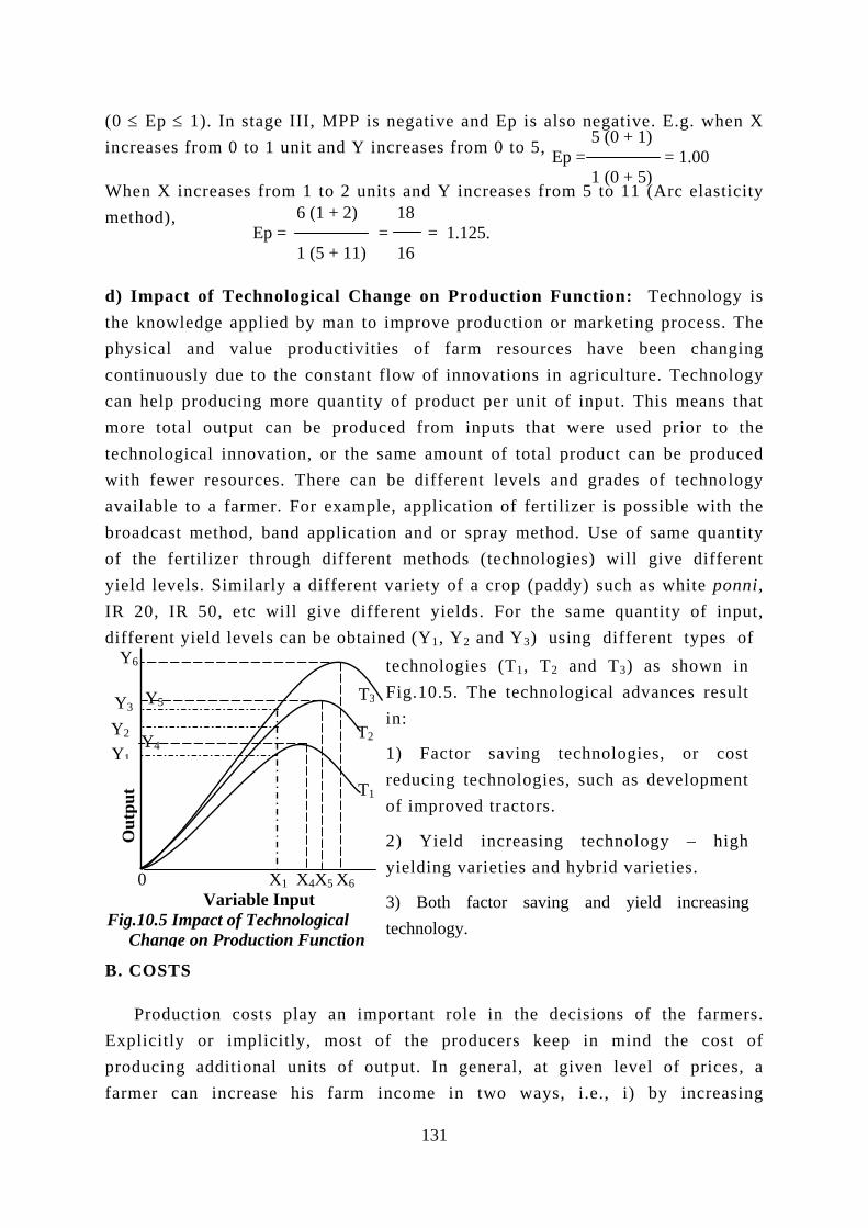
d) Impact of Technological Change on Production the knowledge applied by man to improve productionphysical and value productivities of farm resourcontinuously due to the constant flow of innovations can help producing more quantity of product per unitmore total output can be produced from inputs thatechnological innovation, or the same amount of totawith fewer resources. There can be different levels available to a farmer. For example, application of ferbroadcast method, band application and or spray metof the fertilizer through different methods (technolyield levels. Similarly a different variety of a crop (pIR 20, IR 50, etc will give different yields. For thd erent yield levels can be obtained (Y1, Y2 and Y3)
technologies (T1, TFig.10.5. The technin:
1) Factor saving reducing technologiof improved tractors
2) Yield increasiyielding varieties an
5
3) Both factor savtechnology.
B. COSTS
Production costs play an important role in the Explicitly or implicitly, most of the producers kproducing additional units of output. In general, atfarmer can increase his farm income in two way
131
5 (0 + 1) Ep = = 1.00 1 (0 + 5)
also negative. E.g. w
rom 5 to 11 (Arc ela
6 (1 + 2) 18 Ep = = = 1.125.s from 1 to 2 units and Y incre
1 (5 + 11) 16
Function: Technology is or marketing process. The ces have been changing in agriculture. Technology of input. This means that t were used prior to the l product can be produced and grades of technology tilizer is possible with the hod. Use of same quantity ogies) will give different addy) such as white ponni, e same quantity of input, using different types of
2 and T3) as shown inological advances result
YY2
technologies, or cost
Y1T3
T2
es, such as development.
T1
ng technology – highd hybrid varieties.
ing and yield increasing
0 X1 X4X5 X6 Variable Input Fig.10.5 Impact of TechnologicalChange on Production Function
Y4
Y
Y6
iff
decisions of the farmers. eep in mind the cost of given level of prices, a s, i.e., i) by increasing
production and / or ii) by reducing the cost of production. Since cost minimization is an individual skill, degree of success in this direction directly adds to the profits of the farm.
Costs refer to the money value of effort extended or sacrifice made in producing an article or rendering a service or achieving a specific purpose. Costs, thus, are the expenses incurred in organizing and carrying out the production process. They include outlays of funds for inputs and services used in production. Money value of all inputs used in the production process is termed as the total cost. If the inputs used are represented by X1, X2,..., Xn and the respective prices by Px1, Px2, ..., Pxn, then the total cost (TC) can be expressed as: TC = Px1.X1 + Px2.X2 + ... + Pxn Xn.
Cos
t (R
s)
TC
TVC
TFC
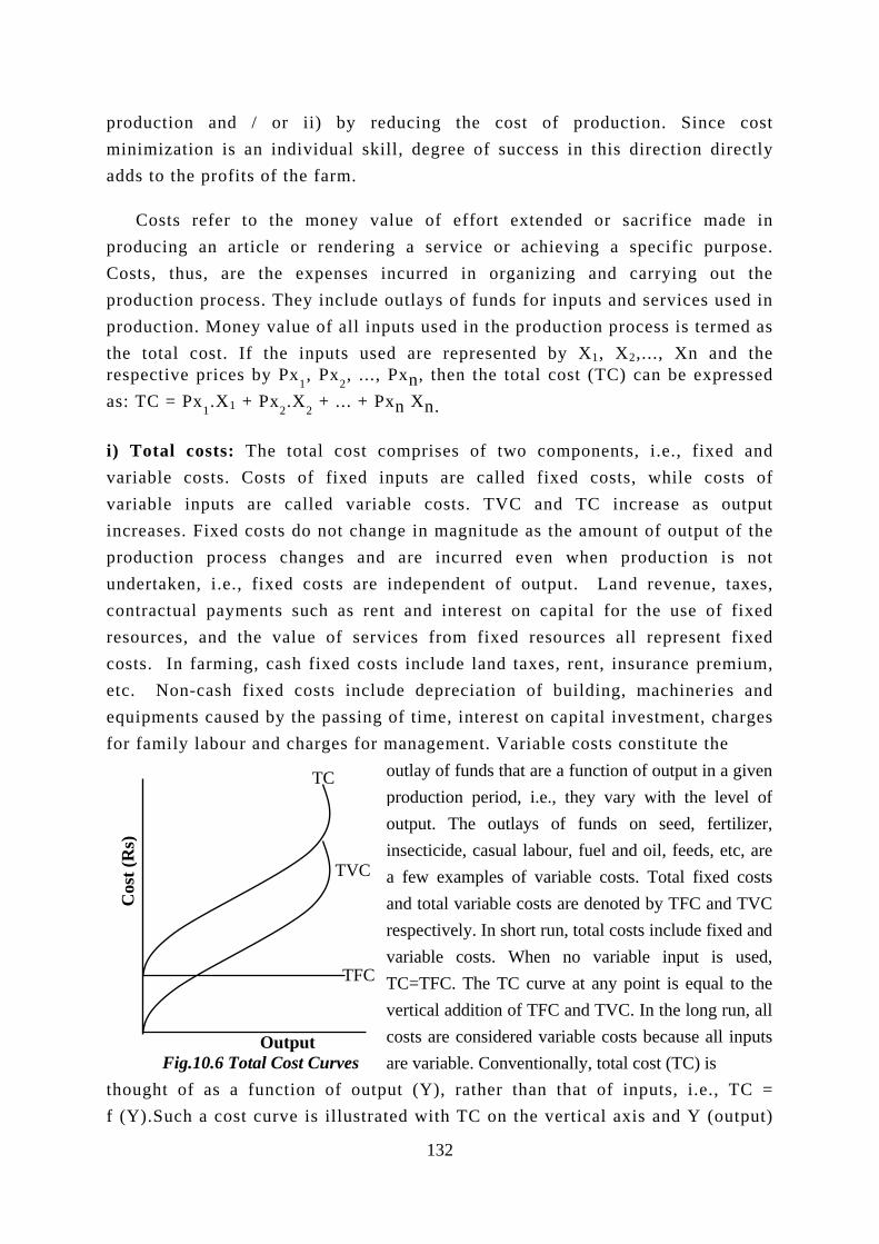
i) Total costs: The total cost comprises of two components, i.e., fixed and variable costs. Costs of fixed inputs are called fixed costs, while costs of variable inputs are called variable costs. TVC and TC increase as output increases. Fixed costs do not change in magnitude as the amount of output of the production process changes and are incurred even when production is not undertaken, i.e., fixed costs are independent of output. Land revenue, taxes, contractual payments such as rent and interest on capital for the use of fixed resources, and the value of services from fixed resources all represent fixed costs. In farming, cash fixed costs include land taxes, rent, insurance premium, etc. Non-cash fixed costs include depreciation of building, machineries and equipments caused by the passing of time, interest on capital investment, charges for family labour and charges for management. Variable costs constitute the
outlay of funds that are a function of output in a givenproduction period, i.e., they vary with the level ofoutput. The outlays of funds on seed, fertilizer,insecticide, casual labour, fuel and oil, feeds, etc, area few examples of variable costs. Total fixed costsand total variable costs are denoted by TFC and TVCrespectively. In short run, total costs include fixed andvariable costs. When no variable input is used,TC=TFC. The TC curve at any point is equal to thevertical addition of TFC and TVC. In the long run, allcosts are considered variable costs because all inputsare variable. Conventionally, total cost (TC) is
thof (Y
Output Fig.10.6 Total Cost Curves
ught of as a function of output (Y), rather than that of inputs, i.e., TC = ).Such a cost curve is illustrated with TC on the vertical axis and Y (output)
132
on the horizontal axis. The total cost curve is similar to the production curve, when the physical units of X (input) have been replaced with the corresponding cost (PxX). Hence, the shape of the TC curve, like that of the TVC curve,
depends upon the production function. In symbolic notation, TC can be written as:
TC = TFC + TVC = TFC + Px X, where TVC = PxX.
ii) Average Fixed Cost, Average Variable Cost and Average Total Cost a) Average Fixed Costs (AFC): Average fixed costs, (AFC) are computed by dividing total fixed costs by are amount of output. AFC varies depending on the amount of production.
b) Average variable cost, Aby the amount of output. AThe shape of the AVC curvewhile AFC always has the sam
c) Average Variable Cost cost is inversely related to aAVC is decreasing. When APWhen APP is decreasing, AAPP measures the efficiency measure for cost curves. Whinput is increasing; efficiencand is decreasing when AVCfollows:
TVC PxX AVC = = Y Y
d) Average Total Costs, ATbe divided by output or AFC
ATC = TC / Y. (or) ATC =
e) Nature and Relationship depends upon the shape of tincreases from zero, attainsreferred to as unit cost of poutput. The initial decrease
TFCAFC = Y
VC: It is computed by dividing total variable cost VC varies depending on the amount of production. depends upon the shape of the production functione shape regardless of the production function.
and Average Physical Product: Average variable verage physical product. When APP is increasing, P is at its maximum, AVC attains a minimum value. VC is increasing. Thus, for a production function, of the variable input, while AVC provides the same en AVC is decreasing, the efficiency of the variable y is at a maximum level when AVC is a minimum is increasing. The relationship algebraically is as
X Px X 1 = Px = , because = Y APP Y APP
C: It can be computed in two ways. Total costs can and AVC can be added.
AFC+AVC.
between Cost Curves: The shape of the ATC curve he production function. ATC decreases as output a minimum, and increases thereafter. ATC is roduction, i.e., the cost of producing one unit of in ATC is caused by the spreading of fixed costs
133

MC ATC
AVC
AFC
Cos
t (R
s)
among an increasing number of unitsof output and the increasingefficiency with which the variableunits is used (as indicated by thedecreasing AVC curve). As outputincreases further, AVC attains aminimum and begins to increase;when these increases in AVC can nolonger be offset by decreases in AFC,ATC begins to rise. AVC reaches itslowest point earlier than ATC.
Output Fig.10.7 Average and Marginal Cost Curves
iii) Marginal Cost, MC: It is defined as the change in total cost per unit increase in output. It is the cost of producing an additional unit of output. MC is computed by dividing the change in total costs, ∆TC, by the corresponding change in output, ∆Y, i.e., MC =∆TC / ∆Y. By definition, the only change possible in total costs is the change in variable cost, because fixed cost does not vary as output varies. Thus, ∆TC =∆TVC. Therefore, MC could also be computed by dividing the change in total variable cost by the change in output. Geometrically, MC is the slope of the TC and the TVC curve. The shape of the MC curve is in an inverse relationship to that of MPP. For lower levels of output, MC is decreasing while MPP is increasing. Algebraically, the relationship betwe
MC and AVC areMC is less than AAVC and ATC. output greater thato ATC at the laATC curves at the
Costs need be
stages I and II o
rational manager
and continues to t
TC = 100 + 8Y
TFC = 100
∆ TC ∆TVC Px (∆X) ∆X Px MC = = = = Px . = ∆Y ∆ Y ∆Y ∆Y MPP
en MPP and MC can be shown as:
equal, where MPP is equal to APP. For lower output levels, VC and ATC and for higher output levels, MC is greater than
As long as there is some fixed costs, MC crosses ATC at an n the output at which AVC is at the minimum and MC is equal tter’s minimum point. MC curve will intersect the AVC and ir lowest point from below.
computed and graphed for input and output amounts only in
f the production function; stage III is an area in which no
would produce. Stage II begins at the point where MC=AVC
he point where output is a maximum.
- 0.4Y2 + 0.02Y3
134
TVC = 8Y - 0.4Y2 + 0.02Y3
AVC = TVC = 8 – 0.4Y + 0.02Y2
Y AFC = TFC = 100 Y Y ATC = AFC + AVC = 100Y-1 + 8 – 0.4 Y + 0.02Y2
MC = dTVC = 8 – 0.8 Y + 0.06Y2 dY
iv) Methods of Determining the Optimum Level
The problem here is to determine the most profitable point of operation for an enterprise in the short-run. This can be done by determining either the most profitable amount of input or the most profitable level of output. As the production function relates the input to output in a unique manner in stage II, either method results ultimately the same answer. In economic terminology, the “most profitable” amount can be called the “optimum” amount. a) Determining the Optimum using Total Value Product and Total Costs: Total Value Product, TVP, is the total value of the production of an enterprise. TVP = Py. Y, where Py is the price per unit of the output and Y is the amount of output at any level of input X. Total value product minus total cost is the profit which is also called net returns or net revenue. As output increases, profit increases and reach a maximum of Rs.30 at 8 units of input and 28 units of output as could be seen from the table 10.4. Maximum profit from an enterprise does not necessarily occur where output is at its maximum. Output reaches a maximum of 29 units at 9 units of input. Therefore, the point of maximum yield is not necessarily the same as the point of maximum profit. Profit = TVP – TC = TVP –TVC – TFC = Py.Y – Px X – TFC.
b) Determining the Optimum Amount of Input
The criterion for determining the optimum amount of input is derived from the slopes of total value product and total cost curves, when those curves are plotted as functions of the input, X. First, consider the profit equation as the function of input.
Profit = Py. f(X) – Px X – TFC, where, Y = f(X).
d (Profit) dY
In order to maximize this function with respect to the variable input, the first derivative is set to zero as follows:
= Py Px = 0 dX dX
= Py.MPP – Px = 0 Py.MPP = Px , i.e., VMP = Px.
135
But, the term Py. MPP is the slope of TVP curve and is called the Value of Marginal Product (VMP). The term Px is the slope of the total cost function. In
etition, Px will always be constant. Dividing both sides of Py, we get,
. So, another method of stating the marginal criterion is to say that
the marginal product of variable input must equal the inverse ratio of prices (input - output price ratio).
c) Determining the Optimum Amount of Output
The marginal conditions for the maximization of profit as a function of output can be derived from the following profit function:
Profit = TR – TC = Py.Y – Px. X – TFC =Py.Y – Px.f -1 (Y) – TFC
d (profit) dX = Py – Px = 0 d Y dY Px = Py – = 0 MPP Px Py = MC⋅ Since MC =
where, the concept of the inverse production function must be used to express X as a function of Y. That is, X = f -1 (Y) in stages I and II. Taking the derivatives of profit with respect to Y results in:
MPP
.d ( Profit) d TR d TC = − = 0
Therefore, Py = MC at the optimum output level. Differentiation of profit equation with respect to Y would give
d Y dY dY d TR d TC = i.e., MR=MC d Y dY
where, the change in TR with respect to Y is defined as Marginal Revenue, MR, while the change in TC with respect to Y is the Marginal Cost, MC. In pure competition Py = MR. d) Comparison of Input and Output Criteria: All methods of determining the most profitable level of output or input lead to comparable answers. The input criterion VMP = Px can be written as Py. MPP = Px (or)
∆ Y Py. = Px . That is, Py. ∆Y = Px. ∆X ∆ X
Px MPP =
pure comp
Py
136

Input (Units)
Total Output (Units)
Average Product =Y/X (Units)
Marginal Product = ∆Y/∆X (Units)
Total Fixed Costs (TFC) (Rs)
Total Variable Cost (TVC) @ Rs.2/Unit
Total Cost=TFC+TVC (Rs)
Average Fixed Cost (AFC) =TFC/Y
Average Variable Cost (AVC) = TVC/Y
Average Total Cost (ATC) = TC/Y
Marginal Cost (MC) =∆TC/∆Y
Marginal Revenue (MR) =∆TR/∆Y
0 0 0 0 10 0 10 0 0 0 - -
1 2 2.00 2 10
2 12 5.00 1.00 6.00 1.00 2
2 5 2.50 3 10 4 14 2.00 0.80 2.80 0.67 2
3 9 3.00 4 10 6 16 1.11 0.67 1.78 0.50 2
4 14 3.50 5 10 8 18 0.71 0.57 1.28 0.40 2
5 19 3.80 5 10 10 20 0.53 0.53 1.06 0.40 2
6 23 3.83 4 10 12 22 0.43 0.52 0.95 0.50 2
7 26 3.71 3 10 14 24 0.38 0.54 0.92 0.67 2
8 28 3.50 2 10 16 26 0.36 0.57 0.93 1.00 2
9 29 3.22 1 10 18 28 0.34 0.62 0.96 2.00 2
10 29 2.90 0 10 20 30 0.34 0.69 1.03 - 2
11 28 2.55 -1 10 22 32 0.36 0.79 1.15 - 2
12 26 2.17 -2 10 24 34 0.38 0.92 1.30 - 2
Table 10.4 Product-Cost Relationships
137
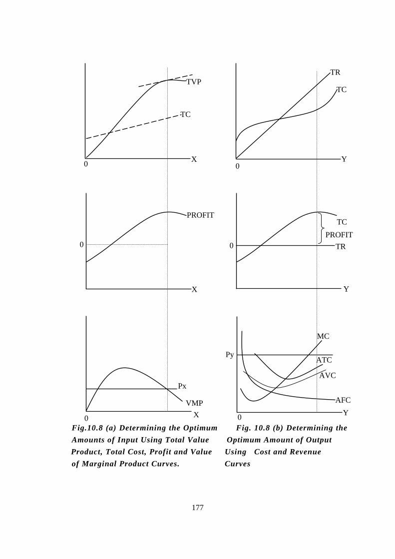
P
Fig.10.8 (a) Determining the Amounts of Input Using Tota
Product, Total Cost, Profit anof Marginal Product Curves.
TV
C
TOl d
X
177
P
ptimum Fig. 10.8 (b) DetermininValue Optimum Amount of Outpu Value Using Cost and Revenue Curves
TR
C
gt
TC
t
Y
PROFIT
T
X
TC
TRO
PR FIXM
Px
V
h
YF
MC
Py
ATAVC
A C
0
0
00
0
0Y
e
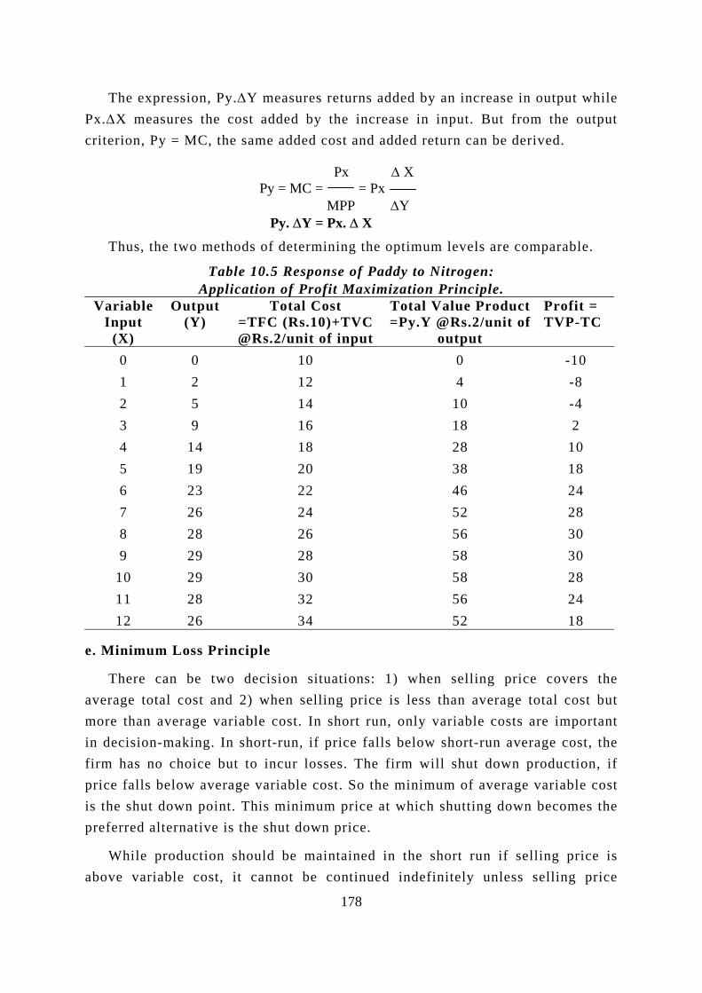
The expression, Py.∆Y measures returns added by an increase in output while Px.∆X measures the cost added by the increase in input. But from the output criterion, Py = MC, the same added cost and added return can be derived.
178
Px ∆ X Py = MC = = Px MPP ∆Y Py. ∆Y = Px. ∆ X
Thus, the two methods of determining the optimum levels are comparable.
Table 10.5 Response of Paddy to Nitrogen: Application of Profit Maximization Principle.
Variable Input
(X)
Output (Y)
Total Cost =TFC (Rs.10)+TVC @Rs.2/unit of input
Total Value Product =Py.Y @Rs.2/unit of
output
Profit = TVP-TC
0 0 10 0 -10 1 2 12 4 -8 2 5 14 10 -4 3 9 16 18 2 4 14 18 28 10 5 19 20 38 18 6 23 22 46 24 7 26 24 52 28 8 28 26 56 30 9 29 28 58 30
10 29 30 58 28 11 28 32 56 24 12 26 34 52 18
e. Minimum Loss Principle
There can be two decision situations: 1) when selling price covers the average total cost and 2) when selling price is less than average total cost but more than average variable cost. In short run, only variable costs are important in decision-making. In short-run, if price falls below short-run average cost, the firm has no choice but to incur losses. The firm will shut down production, if price falls below average variable cost. So the minimum of average variable cost is the shut down point. This minimum price at which shutting down becomes the preferred alternative is the shut down price.
While production should be maintained in the short run if selling price is above variable cost, it cannot be continued indefinitely unless selling price
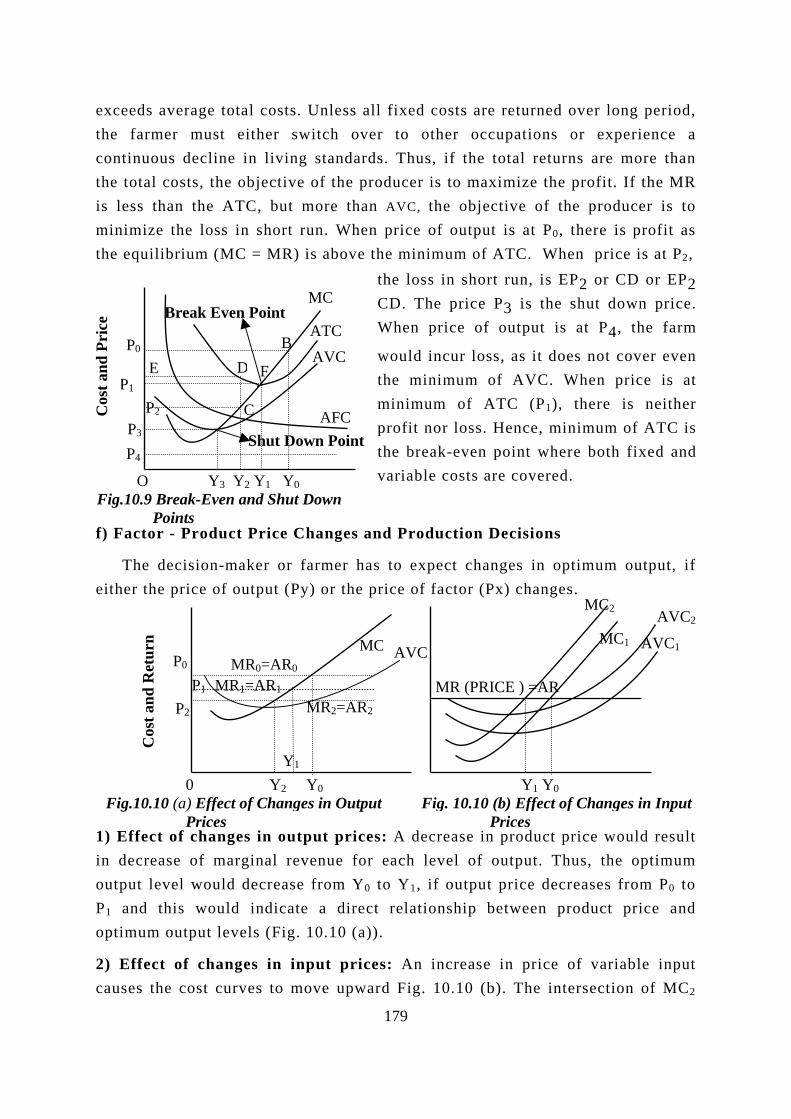
Fig
C
Break Even Point
exceeds average total costs. Unless all fixed costs are returned over long period, the farmer must either switch over to other occupations or experience a continuous decline in living standards. Thus, if the total returns are more than the total costs, the objective of the producer is to maximize the profit. If the MR is less than the ATC, but more than AVC, the objective of the producer is to minimize the loss in short run. When price of output is at P0, there is profit as the equilibrium (MC = MR) is above the minimum of ATC. When price is at P2,
the loss in short run, is EP2 or CD or EP2CD. The price P3 is the shut down price.When price of output is at P4, the farm
would incur loss, as it does not cover even
Cos
t and
Pri
ce
f) F
eith
Fi
1) Ein outP1 opt
2) cau
P0
O.10.
the minimum of AVC. When price is at
ac
Ther
g.10
ffdecputandimu
Effses
E
P1minimum of ATC (P1), there is neither
P2profit nor loss. Hence, minimum of ATC is
P3the break-even point where both fixed and
P4Y3 Y2 Y1 Y0 9 Break-Even and Shut Points tor - Product Price C
e decision-maker or fthe price of output (Py
0 Y2 .10 (a) Effect of Chang
Prices
1
Cos
t and
Ret
urn
ect of changes in outrease of marginal re level would decrease this would indicatm output levels (Fig.
ect of changes in in the cost curves to m
MC
e
v
e
ATC
D
p
o
AV
h
a)
Ys
e f 1
p
AFC
B
F
DC
Shut Down Point
own variable costs are covered.
anges and Production Decisions
rmer has to expect changes in optimum output, if or the price of factor (Px) changes.
2
P0
MR (PRICE ) =AR
P1P2
0 in Ou ut prnue rom a di
0.10
ut prve up
MC
1
tput ices:for eY0 torect (a)).
icesward
AVC
Y
MR0=AR0MR2=AR2
79
Y1 Y0 Fig. 10.10 (b) Effect of Ch Prices A decrease in product priceach level of output. Thus, Y1, if output price decreasrelationship between produ
: An increase in price of v Fig. 10.10 (b). The interse
MC1
anges i
woul the oes fromct pri
ariablction
AVC2AVC1
AV
MC2n
dp
c
eo
C
MR1=AR1
MR0=A
R0Input
result timum P0 to e and
input f MC2
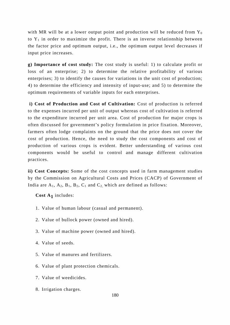
180
with MR will be at a lower output point and production will be reduced from Y0 to Y1 in order to maximize the profit. There is an inverse relationship between the factor price and optimum output, i.e., the optimum output level decreases if input price increases.
g) Importance of cost study: The cost study is useful: 1) to calculate profit or loss of an enterprise; 2) to determine the relative profitability of various enterprises; 3) to identify the causes for variations in the unit cost of production; 4) to determine the efficiency and intensity of input-use; and 5) to determine the optimum requirements of variable inputs for each enterprises.
i) Cost of Production and Cost of Cultivation: Cost of production is referred to the expenses incurred per unit of output whereas cost of cultivation is referred to the expenditure incurred per unit area. Cost of production for major crops is often discussed for government’s policy formulation in price fixation. Moreover, farmers often lodge complaints on the ground that the price does not cover the cost of production. Hence, the need to study the cost components and cost of production of various crops is evident. Better understanding of various cost components would be useful to control and manage different cultivation practices.
ii) Cost Concepts: Some of the cost concepts used in farm management studies by the Commission on Agricultural Costs and Prices (CACP) of Government of India are A1, A2, B1, B2, C1 and C2, which are defined as follows:
Cost A1 includes:
1. Value of human labour (casual and permanent).
2. Value of bullock power (owned and hired).
3. Value of machine power (owned and hired).
4. Value of seeds.
5. Value of manures and fertilizers.
6. Value of plant protection chemicals.
7. Value of weedicides.
8. Irrigation charges.
181
9. Land revenue and other taxes.
10. Depreciation on farm implement and farm buildings.
11. Interest on working capital.
12. Other miscellaneous expenses.
The following concepts can be used for easy calculation of the cost of cultivation.
1) Depreciation for buildings: 2 per cent for pucca building; 5 per cent for tiled building and 10 per cent for katcha building.
2) Depreciation for implements: 10 per cent for major implements and 20 per cent for minor implements.
3) Depreciation for cattle: Appreciation in the value of animals during the first 3 years would be at the ratio of 1:3:5.It remains constant during 4th and 5th year. Then it is assumed that the value of animal depreciates @ 12.5 per cent per year from 6th to 14th year in straight-line method.
4) Interest on working capital: 12 per cent per annum or opportunity cost of capital.
Cost A2 = Cost A1 + Rent paid for leased in land.
Cost B1 = Cost A1 + Interest on the value of owned capital assets (excluding
land).
Interest rate of long - term government floated loans or securities: 10 per cent.
Cost B2 = Cost B1 + Rental value of owned land (less land revenue) and Rent
paid for leased in land.
Cost C1 = Cost B1 + Imputed value of family labour.
Cost C2 = Cost B2 + Imputed value of family labour.
iii) Income measures in relation to different cost concepts
1. Farm Business Income = Gross Return - Cost A1.
2. Owned Farm Business Income = Gross Return - Cost A2.

182
3. Family Labour Income = Gross Return - Cost B2.
4. Net Income = Gross Return - Cost C2.
5. Farm Investment Income = Net Income + Imputed rental value of owned land + Interest on fixed capital.
iv) Opportunity Cost
Every resource used in the production process has but one true cost; its opportunity cost. The opportunity cost of a resource is the return, the resource can earn when put to its best alternative use. Suppose, a farmer applies fertilizer (50 kgs) to paddy will add Rs.500 and application of fertilizer (50 kgs) to sugarcane would add Rs.600. Now, if he fertilizes sugarcane, the opportunity cost of fertilizer is Rs.500; he has foregone Rs.500 to earn Rs.600. Every resource used in the production process, thus, has but one true cost; opportunity cost, the next best alternative foregone.
v) Economic Efficiency
Economic efficiency refers to the combinations of inputs that maximize an individual’s objectives. Economic efficiency is defined in terms of two conditions, namely, necessary and sufficient.
a) Necessary condition: This condition is met in a production process where there is (1) no possibility of producing the same amount of product with fewer inputs (reducing one or more resources) and (2) no possibility of producing more product with the same amount of inputs. In production function analysis, this condition is met in stage II; that is, when the elasticity of production is equal to or greater than zero and is equal to or less than one (0 ≤ εp ≤ 1). The necessary condition refers only to the physical relationship. It is universal because it is applicable in any economic system. No one would knowingly produce in stage III because the same or larger output could be obtained by moving to stage II with lesser input. In a given input-output relationship, many input-output combinations will satisfy the necessary condition. For this reason, an additional condition is needed to single out one alternative from the many that meet the necessary condition.
b) Sufficient Condition: Unlike the necessary condition, which is objective, the sufficient condition for efficiency encompasses individual or social goals and values. In abstract theory, the sufficient condition is often called a choice
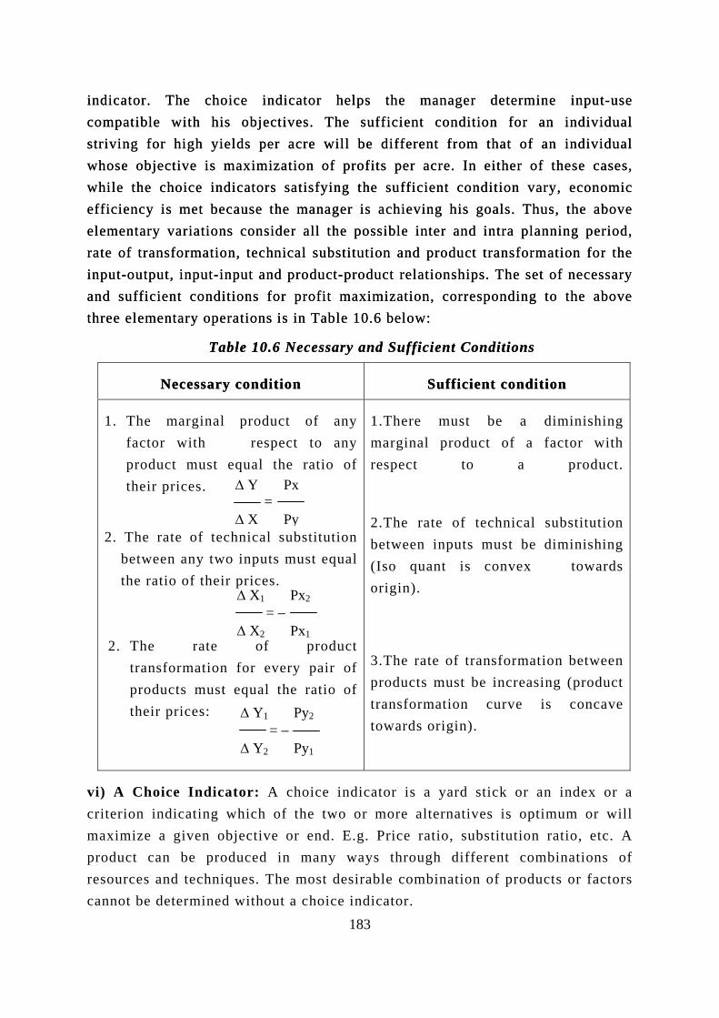
indicator. The choice indicator helps the manager determine input-use compatible with his objectives. The sufficient condition for an individual striving for high yields per acre will be different from that of an individual whose objective is maximization of profits per acre. In either of these cases, while the choice indicators satisfying the sufficient condition vary, economic efficiency is met because the manager is achieving his goals. Thus, the above elementary variations consider all the possible inter and intra planning period, rate of transformation, technical substitution and product transformation for the input-output, input-input and product-product relationships. The set of necessary and sufficient conditions for profit maximization, corresponding to the above three elementary operations is in Table 10.6 below:
indicator. The choice indicator helps the manager determine input-use compatible with his objectives. The sufficient condition for an individual striving for high yields per acre will be different from that of an individual whose objective is maximization of profits per acre. In either of these cases, while the choice indicators satisfying the sufficient condition vary, economic efficiency is met because the manager is achieving his goals. Thus, the above elementary variations consider all the possible inter and intra planning period, rate of transformation, technical substitution and product transformation for the input-output, input-input and product-product relationships. The set of necessary and sufficient conditions for profit maximization, corresponding to the above three elementary operations is in Table 10.6 below:
Table 10.6 Necessary and Sufficient Conditions Table 10.6 Necessary and Sufficient Conditions
Necessary condition Necessary condition Sufficient condition Sufficient condition
1. The marginal product of any factor with respect to any product must io of their prices.
2. The rate of tec
between any twothe ratio of their
2. The rate transformationproducts must their prices:
1.There must be a diminishing marginal product of a factor with respect to a product.
2.The rate of technical substitution
vi) A Choice Indicacriterion indicating wmaximize a given obproduct can be proresources and techniqcannot be determined
∆ Y Px = ∆ X Py
equal the rat
hnical substitution inputs must equal
between inputs must be diminishing (Iso quant is convex towards origin).
d
∆ X1 Px2
= − ∆ X2 Px1
prices.
of product for every pair of
of
3.The rate of transformation between products must be increasing (product transformation curve is concave towards origin).
t
u
equal the ratio∆ Y1 Py2
= − ∆ Y2 Py1
183
or: A choice indicator is a yard stick or an index or a hich of the two or more alternatives is optimum or will
jective or end. E.g. Price ratio, substitution ratio, etc. A uced in many ways through different combinations of es. The most desirable combination of products or factors
without a choice indicator.
a) Optimum Input: Py MPP = Px (or) VMP = Px
b) Optimum Output: Py = MC
c) Least Cost Combination:
d) Maximum Revenue Yieldin
A choice must be made withusually expressed in monetary terlikes and dislikes of the farmers. Fmight ask himself whether paddy ias much as a competing crop, production economics, the commeconomic efficiency, which womaximization.
Chapter 10: Questions for Review
1. Fill up the following:
i) The co-efficient of elasticity of the second stage of production.
ii) Average physical product is invinversely related to marginal cost.
iii) Law of diminishing marginal rechange in .
iv) MPP =APP, when APP is at its
v) Slope of the total physical produ
vi) MC cuts AVC at its lev
vii) In the short run, the objective
viii) Gross return is equal to total
ix) When output increases, the ave
x) The ratio between MPP and APP
∆X1 Px2 MPPx2y = = ∆X2 Px1 MPPx1y
g Combination:
the help of anms, but could beor example, whis yielding the ret
say irrigated gonly assumed guld subsume th
:
production range
ersely related to
turns will not op
level.
ct is indicated b
el.
in farming shoul
production times
rage fixed cost
is called
184
∆Y1 Py2 MPPxy1 = = ∆Y2 Py1 MPPxy2
indicator listed above. It is any other index that reflects
le making a decision, a farmer urn twice as much or one-half round-nut. In the study of oal of the farm manager is e narrower goal of profit
s from to in
, while is
erate, unless there is a
y .
d be to cover cost.
.
continuously.
.

185
2. Define the following:
i) Cost.
ii) Optimum Input level and Optimum Output level.
iii) Average Variable Cost.
iv) Marginal cost and Marginal revenue.
v) Elasticity of production.
vi) Opportunity Cost.
vii) Cost of cultivation and Cost of production.
viii) Law of increasing returns and law of constant returns.
ix) Physical optimum and Economic optimum.
x) Value of Marginal Product.
xi) Choice indicator.
3.Write short notes on the following:
i) Objectives of factor-product relationship
ii) Impact of technological change on production function (or) Impact of improvement in technology on optimum levels of input and output.
iii) Shut down point and Break-even point (or) Minimum loss principle.
iv) Impact of prices of input and output on optimum quantity of output to be produced.
v) Necessary and Sufficient conditions of optimality.
3. Answer the following:
i) Define the law of diminishing marginal returns. Explain the three zones of production function with illustration. How Zone II is rational when compared to the other Zones of production function?
ii) Explain the seven cost curves with suitable illustrations.
iii) Discuss the various components cost of cultivation.
iv) What is the significance studying of cost concepts? How will you derive the following income measures using these cost concepts: a) Farm business income, b) Family labour income and c) Farm investment income?
In factor-product relationship, we studied the situation where only one input is varied and all other variables are held constant. But in most real world situations, two or more inputs are often varied simultaneously. So a farmer must choose the particular combination of inputs which would minimize the cost for a given output level. Thus, the main objective here is minimization of cost at a given level of output. When two or more inputs are variables, a given amount of output may be produced in more than one way, i.e., there is a possibility of substituting one factor (X1) for another (X2) as product level (Y) is held constant. The objectives of factor-factor relationship are i) minimization of cost at a given level of output and ii) optimization of output to the fixed factors through alternative resource-use combinations. In this case, the production function is given by Y = (X1, X2 / X3 ,..., Xn), i.e., the production depends on the amounts of X1 and X2 while the other inputs are held constant.
INP
A. ISOQUANT (OR) ISO PRODUCT CURVE
An isoquant is defined as the locus of all combinations of inputs, X1 and X2, for obtaining a given level of output, say, Y(0). Mathematically, such an isoquant is written as: X1 = f (X2, Y(0)) or X2= f (X1, Y(0)). Some of the important types of isoquants depending upon the degree of substitutability between the inputs, are given in figures below:
i) Linear Isoquant: In this case, two inputs substitute at constant rates. Labour input supplied by different persons substitutes at a constant rate. Ammonium sulphate containing 20.6 per cent nitrogen and urea containing 46 per cent
186
∆ X
FACTOR – FACTOR (OR) UT – INPUT RELATIONSHIP
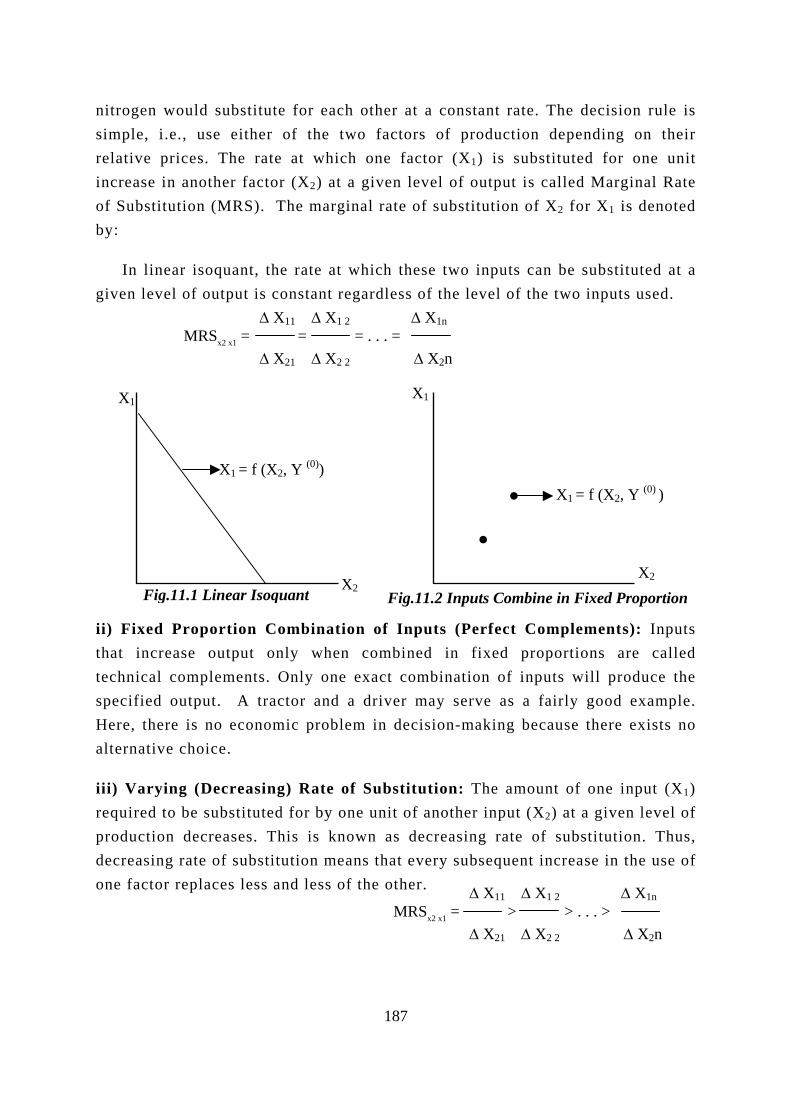
nitrogen would substitute for each other at a constant rate. The decision rule is simple, i.e., use either of the two factors of production depending on their relative prices. The rate at which one factor (X1) is substituted for one unit increase in another factor (X2) at a given level of output is called Marginal Rate of Substitution (MRS). The marginal rate of substitution of X2 for X1 is denoted by:
In linear isoquant, the rate at which these two inputs can be substituted at a given level level of the two inputs used.
ii) Fixed Pthat increatechnical cspecified oHere, therealternative
iii) Varyinrequired toproduction decreasing one factor r
of output is constant regardless of the ∆ X11 ∆ X1 2 ∆ X1nMRSx2 x1 = = = . . . = ∆ X21 ∆ X2 2 ∆ X2n
X1
..
2
Fig.11.2 Inputs Combine in Fixed Proportion
roportion Combinase output only whomplements. Only onutput. A tractor and is no economic probchoice.
g (Decreasing) Rate be substituted for bydecreases. This is k
rate of substitution meplaces less and less
X2
Fig.11.1 Linear IsoquantX1 = f (X2, Y (0))
187
tion of Inputs (Perfect Comen combined in fixed prope exact combination of inpu a driver may serve as a falem in decision-making beca
of Substitution: The amoun one unit of another input (X2
nown as decreasing rate of eans that every subsequent inof the
X1 = f (X2, Y (0) )
X1
plementsortions arts will proirly good use there
t of one in) at a givensubstitutiocrease in t
X
): Inputs e called duce the example. exists no
put (X1) level of n. Thus, he use of
∆ X11 ∆ X1 2 ∆ X1nMRSx2 x1 = > > . . . > ∆ X21 ∆ X2 2 ∆ X2n
other.
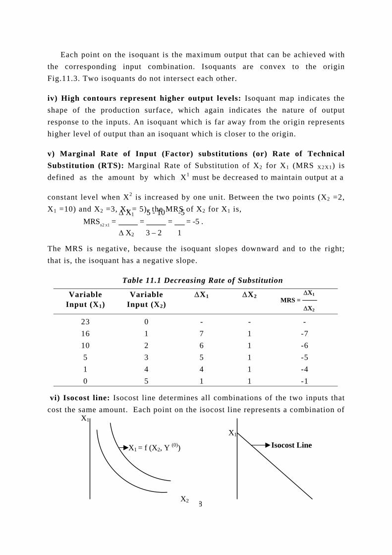
Each point on the isoquant is the maximum output that can be achieved with the corresponding input combination. Isoquants are convex to the origin Fig.11.3. Two isoquants do not intersect each other.
iv) High contours represent higher output levels: Isoquant map indicates the shape of the production surface, which again indicates the nature of output response to the inputs. An isoquant which is far away from the origin represents higher level of output than an isoquant which is closer to the origin.
v) Marginal Rate of Input (Factor) substitutions (or) Rate of Technical Substitution (RTS): Marginal Rate of Substitution of X2 for X1 (MRS X2X1) is defined as the amount by which X1 must be decreased to maintain output at a
∆ X1 5 - 10 -5 MRSx2 x1 = = = = -5 . ∆ X2 3 – 2 1
constant level when X2 is increased by one unit. Between the two points (X2 =2, X1 =10) and X2 =3, X1 = 5), the MRS of X2 for X1 is,
The MRS is negative, because the isoquant slopes downward and to the right; that is, the isoquant has a negative slope.
188
Table 11.1 Decreasing Rate of Substitutio
Variable Input (X1)
Variable Input (X2)
∆X1 ∆X2
23 0 - - 16 1 7 1 10 2 6 1 5 3 5 1 1 4 4 1 0 5 1 1
X1
vi) Isocost line: Isocost line determines all combinations of tcost the same amount. Each point on the isocost line represent
X1
X2
n ∆X1 MRS = ∆X2
- -7 -6 -5 -4 -1
he two inputs that s a combination of
X1 = f (X2, Y (0)) Isocost Line
189
2 Fig.11.3 Convex Isoquant. Fig.11.4 Isocost Line
inputs that can be purchased with the same outlay of funds (Fig.11.4). Uconstant price situation, each possible total outlay has a different isocostAs total outlay increases, isocost line moves higher and higher and moves faaway from the origin. Changes in the input prices will change the sloisocost line as the slope indicates the ratio of input prices. A decrease iinput price means that more of that input can be purchased with the samevariable cost; an increase means that less can be purchased.
Total Outlay = Rs.36; Price of X1 = Rs. 4; Price of X2 = When X1 = 0, X2 = 12; When X2 = 0, X1 = 9.
The equation of the isocost line can be found by solving the TVC equfor X1 as an explic 1 = TVC – Px2X2 and
From this expression, it can be seen that the slope of isocost line is –Px1 while the intercept on X1 is TVC / Px1.
vii) Least cost combination: The problem here is to find out a combinatiinputs, which should cost the least, i.e., minimization of cost. The tangenisocost and isoquant would indicate the least cost combination of X1 and X2
slope of isoquant = sloalgebraically, by equating
Least Cost Combination
coscoudecunof betPx
producing the specified quantity of output can be reduced by using less Xadding X1.
The marginal physical product equations can be used to determine the reper rupee spent at the least cost point. Rewriting the least cost combination
X
nder line. rther
pe of n the total
Rs.3;
ation
TVC Px2 X1= X2 Px1 Px1
it function of X2.Px1X
Px2 /
on of cy of , i.e., iven,
X1
X2
Iso Cost Line
Isoquant
pe of isocost. Least cost combination is gth 1e MRS X2 X to price ratio. ∆ X1 Px2
MRSx2 x1 = = ,i.e., - Px1 (∆ X1) = Px2 (∆ X2) ∆ X2 Px1
Fig.11.5 Least Cost Combination
If - Px1 (∆X1) > Px2 (∆X2), then, thet of producing the given output amountld be reduced by increasing X2 andreasing X1 because the cost of an added
it of X2 is less than the cost of the unitsX1, it replaces. On the other hand, ifween two points of the isoquant,
1 (∆X1) < - Px2 (∆X2), then the cost of
2 and
turns as:
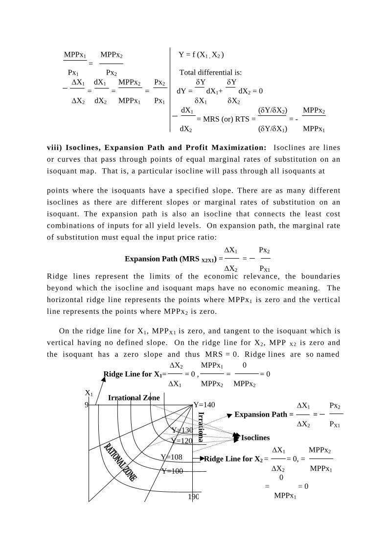
e
viii) Isoclines, Expansion Path and Profit Maximization: Isoclines are lines or curves that pass through points of equal marginal rates of substitution on an isoquant map. That is, a particular isocline will pass through all isoquants at
points where the isoquants have a specified slope. There are as many different isoclines as there are different slopes or marginal rates of substitution on an isoquant. The expansion path is also an isocline that connects the least cost combinations of inputs for all yield levels. On expansion path, the marginal rate of substitution must
Ridge lines represe e, the boundaries beyond which the isocline and isoquant maps have no economic meaning. The horizontal ridge line represents the points where MPPx1 is zero and the vertical line represents the points where MPPx2 is zero.
On the ridge line for X1, MPPX1 is zero, and tangent to the isoquant which is vertical having no defined slope. On the ridge line for X2, MPP X2 is zero and the isoquant h nes are so named
MPPx1 MPPx2 Y = f (X1 , X2 ) = Px1 Px2 Total differential is: ∆X1 dX1 MPPx2 Px2 δY δY = = = dY = dX1+ dX2 = 0 ∆X2 dX2 MPPx1 Px1 δX1 δX2
dX1 (δY/δX2) MPPx2
= MRS (or) RTS = = - dX2 (δY/δX1) MPPx1
X1
1
0
Y=140Ir
rationaY=130
l Z
Y=120one
∆X1 MPPx2Ridge Line for X2 = = 0, =
Y=108 ∆X2 MPPx10
Y=10Irrational Zon
∆X2 MPPx1 0 Ridge Line for X1= = 0 , = = 0 ∆X1 MPPx2 MPPx2
as a zero slope and thus MRS = 0. Ridge li
90
∆X1 Px2Expansion Path = = ∆X2 PX1
Isoclines
∆X1 Px2 Expansion Path (MRS X2X1) = = ∆X2 PX1
equal the input price ratio:
nt the limits of the economic relevanc
9
= = 0 MPPx1
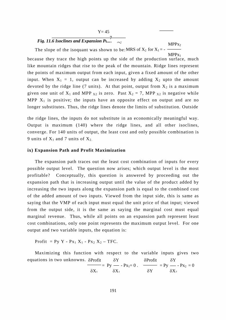
191
The slope of the isoquant was shown t
because they trace the high points up thlike mountain ridges that rise to the peakthe points of maximum output from each input. When X1 = 1, output can be incdevoted by the ridge line (7 units). At thgiven one unit of X1 and MPP X2 is zero.MPP X1 is positive; the inputs have anlonger substitutes. Thus, the ridge lines d
the ridge lines, the inputs do not substituOutput is maximum (140) where the converge. For 140 units of output, the lea9 units of X1 and 7 units of X2.
ix) Expansion Path and Profit Maximiza
The expansion path traces out the leapossible output level. The question nowprofitable? Conceptually, this questionexpansion path that is increasing output increasing the two inputs along the expanof the added amount of two inputs. Viewsaying that the VMP of each input must efrom the output side, it is the same asmarginal revenue. Thus, while all pointcost combinations, only one point represeoutput and two variable inputs, the equati
Profit = Py Y - Px1 X1 - Px2 X2 – TFC
Maximizing this functiequations in two unknowns.
X2
Y= 45
o be
e sid of tinpureasat p
Pas oppenot
te inridg
st co
tion
st co aris is
untilsioned f
qual says onnts ton is
.
MPPx2 MRS of X2 for X1 = - MPPx1
:
e of the production surface, much he mountain. Ridge lines represent t, given a fixed amount of the other ed by adding X2 upto the amount oint, output from X2 is a maximum t X2 = 7, MPP X2 is negative while osite effect on output and are no
e the limits of substitution. Outside
an economically meaningful way. e lines, and all other isoclines, st and only possible combination is
st combination of inputs for every es; which output level is the most answered by proceeding out the
the value of the product added by path is equal to the combined cost rom the input side, this is same as the unit price of that input; viewed ing the marginal cost must equal an expansion path represent least he maximum output level. For one :
o
on with respect to the variable inputs gives tw δProfit δY δProfit δY= Py - Px1= 0 . = Py - Px2 = 0 δX1 δX1 δY δX2
Fig. 11.6 Isoclines and Expansion Path7
The above two equations can be written as: VMPx1 = Px1 (or) VMPx2 = Px2. Thus, the profit-maximizing criterion requires that the marginal earnings of each input must be equal to its cost.
Y = 18X1 - X12 + 14X2 - X22 The marginal physical products of X1 and X2 are multiplied by Py = Rs.
0.65. Then, VMPx1 = (18 - 2X1) 0.65; VMPx2 = (14 - 2X2) 0.65 Equating VMP’s with the input prices of Rs.9 and Rs.7 for X1 and X2
respectively, we get, (18 – 2X1) 0.65 = 9; (14 – 2X2) 0.65 = 7 The solutions are 2.08 for X1 and 1.6 for X2. Substituting these values in the
production function predicts a value of Y equal to 53 units. Then, Profit = 0.65 (53) - 9 (2.08) - 7 (1.60) - TFC= Rs. 4.53 - TFC The optimum criterion for two variable inputs is often expressed as:
A
Rewri
The ab
B. EC
Thproduc‘advanscale rinto i)
i) Inte
Inproduoutpuadvanown eon thethe ef
VMPx1 VMPx2 VMPx1 VMPx2 = 1 ; = 1 or because both equal 1, = = 1 Px1 Px2 Px1 Px2
192
Px1 MPPx1 1 1 MPPx1= ; = = , Since Py =MC Py Px1 Py MC Px2 MPPx2 1 1 MPPx2z= ; = = Py Px2 Py MC
ll variable inputs must be earning as much as they cost on the margin. ting in a different form, yields :
ove expression is the same as MR = MC under perfect competition.
ONOMIES OF SCALE
e scale of production influences the cost of production. In general, larger the scale of tion, the lower is the average cost of production. The term ‘economies’ means tages’ and the term ‘scale’, here, means ‘large-scale production’. Thus, economies of efer to the advantages of large-scale production. Economies of scale can be categorized internal economies and (ii) external economies of scale.
rnal Economies
ternal economies are those economies in production (those reductions in ction costs), which occur in the farm (firm) itself when it expands its t or enlarges its scale of production. Internal economics are those tages that are exclusively available to a particular firm, as a result of its xpansion in the scale of production. The internal economies are dependent resources of the individual house of business, on their organization and
ficiency of their management. Internal economies are of the following five
193
types: a) Technical economies, b) Managerial economies, c) Marketing economies, d) Financial Economies, and e) Risk bearing economies.
a) Technical Economies: A large-scale production unit can use large and modern or sophisticated machines so as to reduce production costs. A large establishment can prevent wastage by utilizing the by-products efficiently. Latest technologies can be used in larger units to reduce the cost of production (E.g.) A big vegetable oil mill can have a cattle feed industry and a big dairy unit.
b) Managerial Economies: These economies arise from the creation of special (separate) departments for different functions like production, maintenance, purchase, sales etc. In a small factory, a manager is a worker, organizer and salesman. Much of his time is wasted on things of little economic importance. In a big concern, such jobs can be allotted to junior employees and the manager can concentrate on jobs which bring more profits. Such kind of division of labour is possible in large units. Thus, the job can be done more efficiently and more economically in large units.
c) Marketing Economies: They arise from the purchase of materials and sale of goods. Large business firms have better bargaining advantages and are provided with a preferential treatment by the firms they deal with. They are able to secure freight concessions from railways and road transport firms, prompt delivery and careful attention from all dealers. A large firm can employ expert purchase managers and sales managers. In selling, it can cut down selling costs and in purchasing, it can have a wider choice.
d) Financial Economies: A big firm has better credit facilities and can borrow on more favourable terms. It encourages prospective investors with incentives and higher returns and therefore, its shares have a wider market. A big firm can issue its shares and debentures more easily than an unknown small firm.
e) Risk-Bearing Economies: A big firm can spread risks and can often eliminate them. It can diversify the output. It can also establish wider marketing net work for its products. If demand for any one of its products slackens in any one market, it may increase it in other markets. Thus, it can reduce the risk of fluctuations in the demand for its product.
ii) External Economies
194
External economies are those economies, which are available to each member firm as a result of the expansion of the industry as a whole. Expansion of industry may lead to the availability of new and cheaper raw materials, machineries and to the use of superior technical knowledge. External economies are advantages available to all the firms. For instance, construction of a new railway line benefits all firms set up in that locality and not to any particular firm alone. Various types of external economies are given below:
a) Economies of concentration: These economies arise from the availability of skilled workers, the provision of better transport and credit facilities, benefits from subsidiary units and so on. Scattered firms cannot enjoy such economies. Concentration of firms enables the transport system to reduce the cost.
b) Economies of Information: All big-sized units can join together to publish trade journals and also to set up research and development facilities, which would benefit all firms.
c) Economies of Disintegration: When an industry grows, it becomes possible to split up some of the processes which are taken up by specialist firms. This may be beneficial to all the firms.
iii) Diseconomies of Scale
Large-scale production also has some disadvantages, which are known as diseconomies of scale. They are as follows: a) If the growth of the firm expands beyond the optimum limit, it will become unwieldy. As a result, the management becomes inefficient. (b) There may be frequent breakdown of machines due to poor maintenance. (c) There may be indiscipline among labourers and this would result in frequent strikes and lock outs. (d) Some times the over production exceeds demand and causes depression and unemployment. (e) The average cost of production will be more.
C. ECONOMIES OF SIZE
A study on economies of size would be useful to assess the optimum size of the plant. The collection of all durable assets owned by a farm is called the plant and this term, therefore, includes land, machinery, buildings and other durable assets found on farms. An increase in any one of these durable assets would increase plant size.
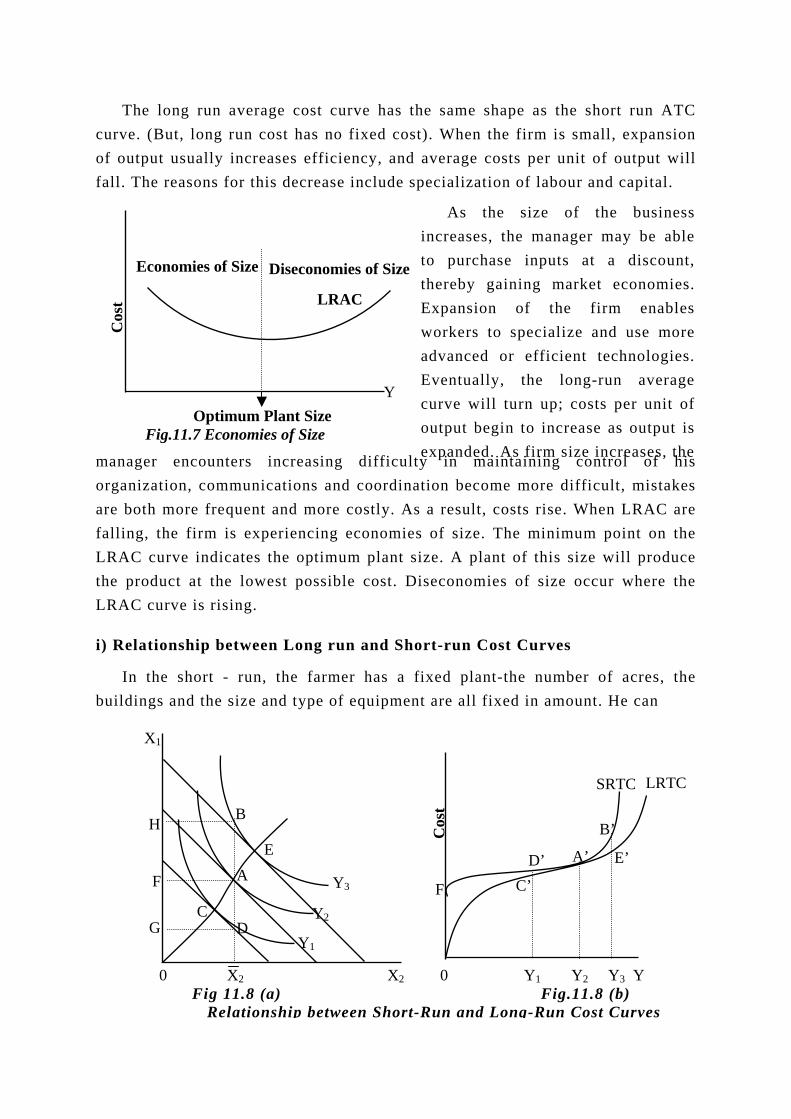
Cos
t
Optimum Plant Size Fig.11.7 Economies of Size
Economies of Size Diseconomies of Size
The long run average cost curve has the same shape as the short run ATC curve. (But, long run cost has no fixed cost). When the firm is small, expansion of output usually increases efficiency, and average costs per unit of output will fall. The reasons for this decrease include spec
incto theExwoadvEvcur
manager encounters increasing diforganization, communications and cooare both more frequent and more costlfalling, the firm is experiencing econLRAC curve indicates the optimum plthe product at the lowest possible coLRAC curve is rising.
i) Relationship between Long run an
In the short - run, the farmer habuildings and the size and type of equi
1
Y
LRAC
outexpficulty
rdination become more difficult, mistakes y. As a result, costs rise. When LRAC are omies of size. The minimum point on the ant size. A plant of this size will produce st. Diseconomies of size occur where the
d Short-run Cost Curves
s a fixed plant-the number of acres, the pment are all fixed in amount. He can
X
ost
C C
B
C
H F G195
0 X2 X2 0 Y1 Y2 Y3 Y Fig 11.8 (a) Fig.11.8 (b) Relationship between Short-Run and Long-Run Cost Curves
E
AC
DY3
Y2
Y1
D’
C’A’
B’
E’
SRT
LRTF
ialization of labour and capital.
As the size of the businessreases, the manager may be ablepurchase inputs at a discount,
reby gaining market economies.pansion of the firm enablesrkers to specialize and use moreanced or efficient technologies.
entually, the long-run averageve will turn up; costs per unit ofput begin to increase as output isanded. As firm size increases, the in maintaining control of his
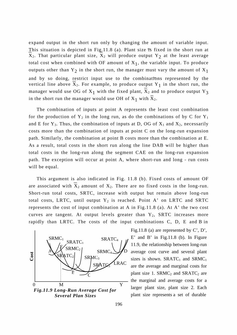
expand output in the short run only by changing the amount of variable input. This situation is depicted in Fig.11.8 (a). Plant size is fixed in the short run at X2. That particular plant size, X2 will produce output Y2 at the least average total cost when combined with OF amount of X1, the variable input. To produce outputs other than Y2 in the short run, the manager must vary the amount of X1
and by so doing, restrict input use to the combinations represented by the vertical line above X2. For example, to produce output Y1 in the short run, the manager would use OG of X1 with the fixed plant, X2 and to produce output Y3 in the short run the manager would use OH of X1 with X2.
The combination of inputs at point A represents the least cost combination for the production of Y2 in the long run, as do the combinations of by C for Y1 and E for Y3. Thus, the combination of inputs at D, OG of X1 and X2, necessarily costs more than the combination of inputs at point C on the long-run expansion path. Similarly, the combination at point B costs more than the combination at E. As a result, total costs in the short run along the line DAB will be higher than total costs in the long-run along the segment CAE on the long-run expansion path. The exception will occur at point A, where short-run and long - run costs will be equal.
Cos
t
This argument is also indicated in Fig. 11.8 (b). Fixed costs of amount OF are associated with X2 amount of X2. There are no fixed costs in the long-run. Short-run total costs, SRTC, increase with output but remain above long-run total costs, LRTC, until output Y2 is reached. Point A’ on LRTC and SRTC represents the cost of input combination at A in Fig.11.8 (a). At A’ the two cost curves are tangent. At output levels greater than Y2, SRTC increases more rapidly than LRTC. The costs of the input combinations C, D, E and B in
Fig.11.8 (a) are represented by C’, D’,E’ and B’ in Fig.11.8 (b). In Figure
SRMC1
11.9, the relationship between long-run
SRATC1average cost curve and several plant
SRMC2sizes is shown. SRATC1 and SRMC1
SRATC2 SRMC3S
3C are the average and marginal costs for
SRATCRMC4
SRATC4
LRA
A
plant size 1. SRMC2 and SRATC2 are
B C196
D
the marginal and average costs for alarger plant size, plant size 2. Eachplant size represents a set of durable
0 M Y Fig.11.9 Long-Run Average Cost for Several Plan Sizes
F
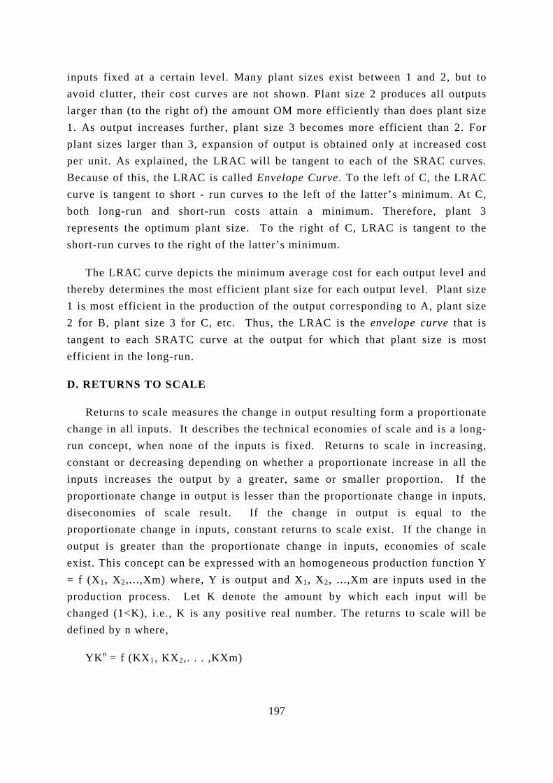
197
inputs fixed at a certain level. Many plant sizes exist between 1 and 2, but to avoid clutter, their cost curves are not shown. Plant size 2 produces all outputs larger than (to the right of) the amount OM more efficiently than does plant size 1. As output increases further, plant size 3 becomes more efficient than 2. For plant sizes larger than 3, expansion of output is obtained only at increased cost per unit. As explained, the LRAC will be tangent to each of the SRAC curves. Because of this, the LRAC is called Envelope Curve. To the left of C, the LRAC curve is tangent to short - run curves to the left of the latter’s minimum. At C, both long-run and short-run costs attain a minimum. Therefore, plant 3 represents the optimum plant size. To the right of C, LRAC is tangent to the short-run curves to the right of the latter’s minimum.
The LRAC curve depicts the minimum average cost for each output level and thereby determines the most efficient plant size for each output level. Plant size 1 is most efficient in the production of the output corresponding to A, plant size 2 for B, plant size 3 for C, etc. Thus, the LRAC is the envelope curve that is tangent to each SRATC curve at the output for which that plant size is most efficient in the long-run.
D. RETURNS TO SCALE
Returns to scale measures the change in output resulting form a proportionate change in all inputs. It describes the technical economies of scale and is a long-run concept, when none of the inputs is fixed. Returns to scale in increasing, constant or decreasing depending on whether a proportionate increase in all the inputs increases the output by a greater, same or smaller proportion. If the proportionate change in output is lesser than the proportionate change in inputs, diseconomies of scale result. If the change in output is equal to the proportionate change in inputs, constant returns to scale exist. If the change in output is greater than the proportionate change in inputs, economies of scale exist. This concept can be expressed with an homogeneous production function Y = f (X1, X2,...,Xm) where, Y is output and X1, X2, ...,Xm are inputs used in the production process. Let K denote the amount by which each input will be changed (1<K), i.e., K is any positive real number. The returns to scale will be defined by n where,
YKn = f (KX1, KX2,. . . ,KXm)
The factor Kn represents the change in output when all inputs are changed by the factor K. For example, if n equals one, the change in output is equal to the changes in the inputs and the returns to scale are constant. If n is greater than one, the change in output exceeds the proportionate change in all the inputs and returns to scale are increasing. Conversely, if n is less than one, the returns to scale are decreasing. In case of constant returns to scale, the distance between successive isoquants is constant, i.e., AB=BC=CD (Fig. 11.10 (a)). The distance goes on widening between isoquants when diminishing returns operate, i.e., AB<BC<CD (Fig.11.10 (b)). Finally, in case of increasing returns to scale, the distance between the successive isoquants becomes smaller and smaller as we move away from the origin on the isoquant map i.e., AB>BC>CD (Fig.11.10 (c)).
Returns to scale must be measured along a scale line, that is a straight line, passing through the origin. Proportionate input changes are possible only on such a line or ray. Thus, economies (diseconomies) of size are the same as economies (diseconomies) of scale only when the long long-run expansion path is a straight line passing through the origin. In most agricultural production situations, input proportions representing least cost combinations vary with the level of output. Therefore, strict interpretations of scale concepts are probably not of great value in agriculture.
X1e
E. ELASTICITY OF FA
In the factor-facdefined as the percentagchange in other input, X
X1
CTOR SUBSTITUTION
tor relationship, the elaste chang
2. Thus,
X1
0 X2 0 X2 0 X2Fig.11.10 (a) Constant Return Fig.11.10 (b) Decreasing Fig.11.10 (c) Increasing to Scale Return to Scale Return to Scale
Y=100 Y=100 Y=100
A
BD
A
BC
D
icity
A
of f
B
act
C
or
D
Y=
200Y=3 00Y=
400Y=175Y=
275Y=400
subs
Y=225Y
titu
=325=400
YScale Lin
tion is tage
198
e in one input, X1, in response to the percen ∆X1
X1 ∆X1X2 X2Es = = = (MRS of X2 for X1) ∆X2 ∆X2X1 X1
X2
C
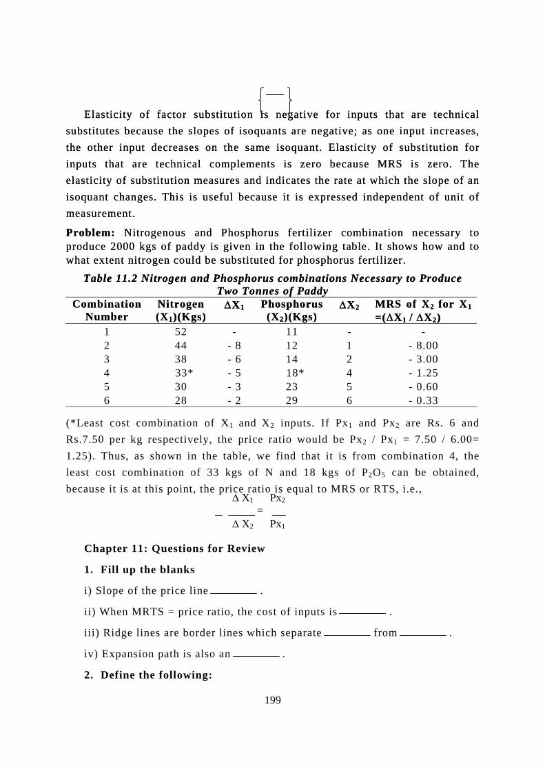
Elasticity of factor substitution is negative for inputs that are technical
substitutes because the slopes of isoquants are negative; as one input increases, the other input decreases on the same isoquant. Elasticity of substitution for inputs that are technical complements is zero because MRS is zero. The elasticity of substitution measures and indicates the rate at which the slope of an isoquant changes. This is useful because it is expressed independent of unit of measurement.
Elasticity of factor substitution is negative for inputs that are technical substitutes because the slopes of isoquants are negative; as one input increases, the other input decreases on the same isoquant. Elasticity of substitution for inputs that are technical complements is zero because MRS is zero. The elasticity of substitution measures and indicates the rate at which the slope of an isoquant changes. This is useful because it is expressed independent of unit of measurement.
Problem: Nitrogenous and Phosphorus fertilizer combination necessary to produce 2000 kgs of paddy is given in the following table. It shows how and to what extent nitrogen could be substituted for phosphorus fertilizer.
Problem: Nitrogenous and Phosphorus fertilizer combination necessary to produce 2000 kgs of paddy is given in the following table. It shows how and to what extent nitrogen could be substituted for phosphorus fertilizer.
Table 11.2 Nitrogen and Phosphorus combinations Necessary to Produce Table 11.2 Nitrogen and Phosphorus combinations Necessary to Produce Two Tonnes of Paddy Two Tonnes of Paddy
Combination Number
Combination Number
Nitrogen (X1)(Kgs) Nitrogen (X
∆X1 Phosphorus (X2)(Kgs)
Phosphorus (X
∆X2 MRS of X2 for X1
=(∆X1 / ∆X2) MRS of X
1)(Kgs) ∆X1
2)(Kgs) ∆X2 2 for X1
=(∆X1 / ∆X2) 1 52 - 11 - - 2 44 - 8 12 1 - 8.00 3 38 - 6 14 2 - 3.00 4 33* - 5 18* 4 - 1.25 5 30 - 3 23 5 - 0.60 6 28 - 2 29 6 - 0.33
(*Least cost combination of X1 and X2 inputs. If Px1 and Px2 are Rs. 6 and Rs.7.50 per kg respectively, the price ratio would be Px2 / Px1 = 7.50 / 6.00= 1.25). Thus, as shown in the table, we find that it is from combination 4, the least cost combination of 33 kgs of N and 18 kgs of P2O5 can be obtained, because it is at this point, the al to MRS or RTS, i.e.,
Chapter 11: Questions fo
1. Fill up the blanks
i) Slope of the price line
ii) When MRTS = price ra
iii) Ridge lines are border
iv) Expansion path is also
2. Define the following:
∆ X1 Px2
= ∆ X2 Px1
price ratio is equ
199
r Review
.
tio, the cost of inputs is .
lines which separate from .
an .
i) Least cost combination. i) Least cost combination.
ii) Elasticity of factor substitution. ii) Elasticity of factor substitution.
iii) Expansion path. iii) Expansion path.
iv) Returns to scale. iv) Returns to scale.
v) Isoproduct / Isoquant curve. v) Isoproduct / Isoquant curve.
vi) Marginal rate of factor substitution. vi) Marginal rate of factor substitution.
vii) Isocost line. vii) Isocost line.
viii) Isocline. viii) Isocline.
ix) Ridge line. ix) Ridge line.
x) Envelope curve. x) Envelope curve.
3. Write short notes on the following: 3. Write short notes on the following:
i) Perfect complements and Perfect substitutes. i) Perfect complements and Perfect substitutes.
ii) Economies of scale and Diseconomies of scale. ii) Economies of scale and Diseconomies of scale.
iii) Relationship between short run and Long run cost curves. iii) Relationship between short run and Long run cost curves.
4. Answer the following: 4. Answer the following:
i) Explain the least cost combination of inputs with illustration. i) Explain the least cost combination of inputs with illustration.
ii) Discuss the internal and external economies of scale. ii) Discuss the internal and external economies of scale.
PRODUCT-PRODUCT (OR) OUTPUT - OUTPUT RELATIONSHIP
In this section, instead of considering the allocation of inputs to an enterprise or among enterprises, we discuss enterprise combinations or product- mix involving product-product relationships. We deal with what combination of enterprises should be produced from a given level of fixed and variable inputs.
In this section, instead of considering the allocation of inputs to an enterprise or among enterprises, we discuss enterprise combinations or product- mix involving product-product relationships. We deal with what combination of enterprises should be produced from a given level of fixed and variable inputs.
A. PRODUCTION POSSIBILITY CURVE (ISO-RESOURCE CURVE) A. PRODUCTION POSSIBILITY CURVE (ISO-RESOURCE CURVE)
200
The production possibility curve or product transformation curve is the locus of maximum amounts of two products, say Y1 and Y2, that can be produced from a given quantity of resources (X(0)). Mathematically, such product transformation curve is represented by: Y1 = f (Y2, X(0) ) or Y2 = f ( Y1, X(0) ). The Rate of Product Transformation (RPT) (or) Marginal Rate Product Substitution (MRPS)
The production possibility curve or product transformation curve is the locus of maximum amounts of two products, say Y1 and Y2, that can be produced from a given quantity of resources (X(0)). Mathematically, such product transformation curve is represented by: Y1 = f (Y2, X(0) ) or Y2 = f ( Y1, X(0) ). The Rate of Product Transformation (RPT) (or) Marginal Rate Product Substitution (MRPS)
dY1 ∆Y1 (Point concept) (or) (Average or arc concept) dY2 ∆Y2
between two products, Y1 and Y2, is given by the negative slope of this curve. The RPT of Y2 for Y1 can either be expressed as:
dY1 / dY2 , the slope of the product transformation curve can be defined as the change (increase or decrease ) in the level of Y1 that must be accompanied by a unit change (decrease or increase ) in the product (Y2) at a given level of resource.
i) Relationship among Products: The basic product relationships can be: joint, complementary, supplementary and competitiveness.
a) Joint Products: Products, which result from the same production process, are termed joint products. In the extreme case, two products are combined in fixed proportions and the production of one without the other is impossible. E.g. Grain and straw. Production possibility curves for joint products of this type are presented in Figure 12.1 (a). No substitution is possible in this case. However, for example, different varieties of paddy produce varying proportions of straw and grain. Thus, the proportions may be changed by technologies or cropping practices usually associated with the fixed inputs. For such products, a narrow range of product substitution may exist as presented in Figure12.1 (b).
.
.
.
0
b) Competitive Products: Products are termed competitive when the output of one product can be increased only by reducing the output of the other product. Outputs are competitive because they require the same inputs at the same time. E.g. the manager can expand production of one output only by diver s-land, labour, capital and management-from one enterprise to another.
A
Fig.12
B
.1 (a)
C
Y120
Y Joint Pr
Y1
1
2 0 oducts Fig.12.1 (b)
∆Y1 ing
< 0 ∆Y2
t input
Y2
∆Y11
∆Y12
∆Y21
∆Y22
When the production concerned are competitiveeither at a constant or incfor another product at a csuch a relationship may ninputs held constant, durinsubstitution. Economic dwould produce only one Whenever a decreasing RPone product, say Y2 repltransformation curve is coThis type of relationship iin very small farms wheretwo competitive commoproduction. Decision-makproduce only one of the twincreasing rate of producboth products are productransformation curve is cY1 must be sacrificed forfor a given level of input.
c) Complementary Produin one product causes an of inpu sed on the two
Y1
∆Y11
202
∆Y21
∆Y22
∆Y12
possibility curve has a n. Two competitive produ
reasing or decreasing rateonstant rate is only a shot hold for long. Two vg any single season provi
ecision-making is easy inof these products dependT exists between two pro
aces less and less of othncave away from origin as quite rare. This type of capital is very limited andities can be extended ing is simple in this co products depending on t transformation betweened in the stage of decr
oncave towards the origin each successive gain of o
1
cts: Two products are coincrease in the second proare held consta
Y1
∆Y11
∆Y21
∆Y22∆Y12
Y2
Y2egative slope, the prodcts can substitute each o. Substitution of one prodort-run phenomenon becaarieties of any crop withde an example of this typ this case, i.e., the faring upon yields and priducts, every unit additioer product, Y1.The prod
nd convex toward the oridecreasing RPT can be fod the produce of none ofbeyond the first stage
ase, i.e., the farmer worelative yields and prices. two products occurs weasing returns. The prod, i.e., increasing amountne unit of other product
mplementary, if an increduct, when the total amo
Y
2Fig.12.2(a)Constant RPTY2Y1.Fig.12.2(b)Decreasing RPTY2Y1.Fig.12.2(c)Increasing RPTY2Y1
∆Y11 ∆Y12 ∆Y1n ∆Y11 ∆Y12 ∆Y1n ∆Y11 ∆Y12 ∆Y1n = =. . . = > >. . . > < < . . . <
∆Y21 ∆Y22 ∆Y2n ∆Y21 ∆Y22 ∆Y2n ∆Y21 ∆Y22 ∆Y2n
ucts ther uct use all e of mer ces. n of uct
gin. und the of uld An hen uct
s of , Y2
ase unt
C
Y1ts u
Ynt.
1
Fig
In the figureached. To theproduce the maof Y2. When lcompetitive. Incomplementarycomplementaryproducts becom
Complemenused by the othwith cash crop.and improve wecash crops thuincrease in theeventually becoyear rotation mproduced only b
d) Supplementamount of one the other. In figzero to OH amotwo outputs supplementary
Supplementa
A
203
.12.3 (a) Complementary
re 12.3(a), Y2 is comple right of A, both are com
ximum possible amount ofarger quantities of Y2 ar Fig.12.3 (b), there is
to the other output to Y1, upto C, and Y1 is e competitive between C a
tary usually occurs when er product. An example o The legume may add nitred and insect control. Thes causing, over a period production of cash crome competitive. For examay be complementary, twoy successive reductions in
ary Products: Two prodcan be increased without ure 12.4 (a) Y2 is supplemunt without affecting the
become competitive. Into the other and competitiv
ry enterprises arise
A
Products Fig.12.3(b)
mentary with Y1 untipetitive. Thus, if the Y1, he should grow at e produced, the two p a situation where
over a certain rangecomplementary to Y2 nd D.
one of the products pf this is the use of a leogen and improve soil se factors, in turn, serv of time required by p. The complementarple, while one year of , three or four yea the cash crops.
ucts are called supplincreasing or decreasinentary to Y1. Y2 can bamount of Y1 produce Fig.12.4 (b), eache between FG.
D
B
Y2l thefarmleastrodueach. T
upto
roducgumstruce as the y pralfal
emeng the incd. Be en
Y2
point A is er wishes to OB amount cts become output is
hus, Y2 is D. The two
es an input e in rotation ture or tilth “inputs” for rotation, an oducts may fa in a four-
ld be
∆Y1 MRPS = > 0. ∆Y2rs of alfalfa cou
tary, if the e amount of reased from yond E, the terprise is
Y
Y1E
E Ft
G
0
0 BBetween EF, Y2 is supplementary to Y1.Between GH, Y1 is supplementary to Y2Be ween FG, Y1 and Y2 are substitutes
through time or when surplus resources are
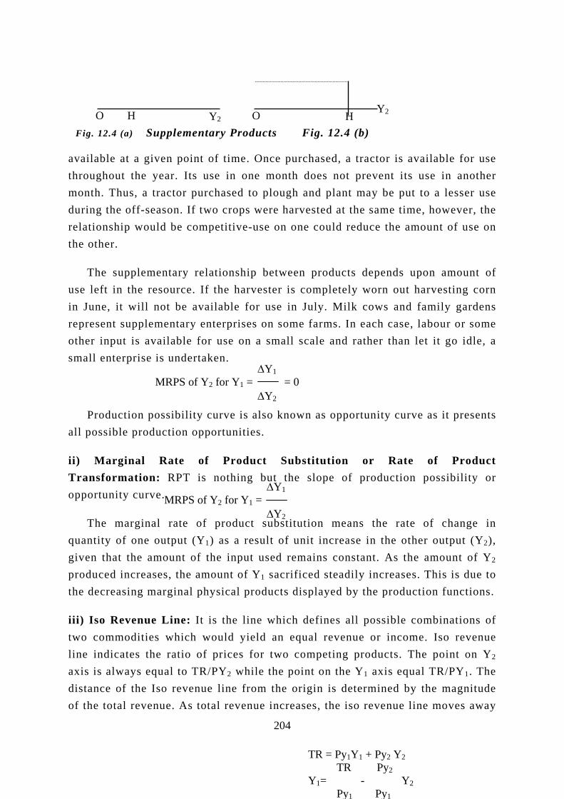
available at a given pointthroughout the year. Its month. Thus, a tractor puduring the off-season. If trelationship would be comthe other.
The supplementary reuse left in the resource. Iin June, it will not be avrepresent supplementary eother input is available fosmall enterprise
Production possibilityall possible production op
ii) Marginal Rate oTransformation:opportunity curve
The marginalquantity of one output (Ygiven that the amount of produced increases, the amthe decreasing marginal p
iii) Iso Revenue Line: Ittwo commodities which wline indicates the ratio ofaxis is always equal to TRdistance of the Iso revenuof the total revenue. As to
Y2
204
of time. Once purchased, a tracuse in one month does not prerchased to plough and plant mawo crops were harvested at the spetitive-use on one could reduc
lationship between products def the harvester is completely wailable for use in July. Milk conterprises on some farms. In ear use on a small scale and rath
curve is also known as opportunportunities.
f Product Substitution ore slope of pro
ution means 1) as a result of unit increase inthe input used remains constanount of Y1 sacrificed steadily i
hysical products displayed by th
is the line which defines all poould yield an equal revenue o
prices for two competing pro/PY2 while the point on the Y1 e line from the origin is determtal revenue increases, the iso re
Y2
H H O Otor is available for use vent its use in another y be put to a lesser use ame time, however, the e the amount of use on
pends upon amount of orn out harvesting corn ws and family gardens
ch case, labour or some er than let it go idle, a
∆Y1 MRPS of Y2 for Y1 = = 0 ∆Y2
is undertaken.
ity curve as it presents
Rate of Product duction possibility or
the rate of change in the other output (Y2),
t. As the amount of Y2 ncreases. This is due to e production functions.
ssible combinations of r income. Iso revenue
ducts. The point on Y2 axis equal TR/PY1. The ined by the magnitude
venue line moves away
TR = Py1Y1 + Py2 Y2 TR Py2 Y1= - Y2 Py1 Py1
∆Y1 MRPS of Y2 for Y1 =
RPT is nothing but th.
∆Y2 rate of product substit
Fig. 12.4 (a) Supplementary Products Fig. 12.4 (b)

from the origin. The slope of the iso revenue line is determined by the output prices.
sirec
iv
c
shshthee
Change in Py1
Y
F
Thus, the gn means tvenue lines
ost minimiza
) Revenue M
The maxi
urve can be d
MRPS of Y2 f
ould be decould be ince line conne
ach level of xpansion pat
1
20
0 Change in Py2 ig.12.5 Iso Revenue Line
output prices ratio is the slohat the iso revenue line sare used for revenue optimtion.
aximizing Combination o
mum revenue combination MR
etermined using the criteri
e
∆Y1 Py2 or Y1 = = - . ∆Y2 Py1
reased in favour of Y1. Wreased at the expense of Ycting maximum revenue poinput, the maximum revenuh.
Y2
pe of the iso revenue line. The negative lopes downward to the right. The iso ization, while iso cost lines are used for
f Outputs
of outputs on the production possibility ∆Y1 Py2
PS of Y2 for Y1 = = - ∆Y2 Py1
on.
Y1
Y2
Production Possibility Curve
Iso Revenue Lin
Fig.12.6 Maximum Revenue Yielding Combination
This can be rewritten as follows: Py1(∆Y1) = - Py2(∆Y2 ). This criterionstates that at the maximum revenue point,the increase in revenue due to adding aminute quantity of Y2 is exactly equal tothe decrease in revenue caused by thereduction in Y1. Thus, there is no incentiveto change the output combination. WhenPy1 (∆Y1) > - Py2 (∆Y2), the amount of Y2
5
hen Py1 (∆Y1) < - Py2 (∆Y2), then Y2 1. As could be seen in the Figure 12.7, ints is called output expansion path. For e combination of outputs will fall on the
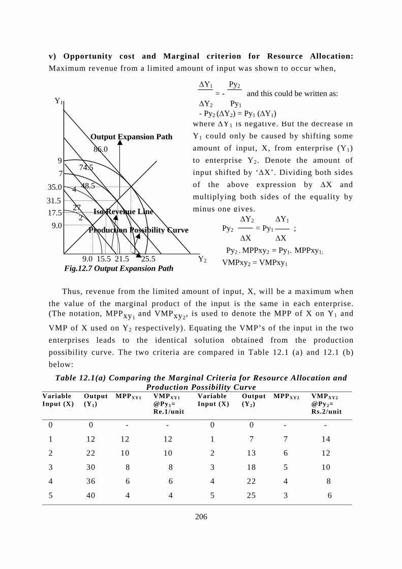
v) Opportunity cost and Marginal criterion for Resource Allocation: Maximum revenue from a limited amount of input was shown to occur when,
1
9Fig.12
Thus, rthe value (The notat
VMP of Xenterprisespossibilitybelow:
Table 12
Variable Input (X)
O(
0
1
2
3
4
5
∆Y1 Py2 = - and this could be written as: ∆Y2 Py1
Output Expansion Path
Y
∆Y2 ∆Y1 Py2 = Py1 ;
e
e
Production Possibility Curv
.0
.7
eoi
.
Y
0
1
2
3
3
4
Iso Revenue Lin
15.5 21.5 25.5 Output Expansion Path
venue from the limited amf the marginal product ofon, MPPxy1 and VMPxy2,
used on Y2 respectively). leads to the identical curve. The two criteria ar
1(a) Comparing the MargProduction
utput 1)
MPPXY1 VMPXY1 @Py1= Re.1/unit
- -
2 12 12
2 10 10
0 8 8
6 6 6
0 4 4
where ∆Y1 is negative. But the decrease inY1 could only be caused by shifting someamount of input, X, from enterprise (Y1)to enterprise Y2. Denote the amount ofinput shifted by ‘∆X’. Dividing both sidesof the above expression by ∆X andmultiplying both sides of the equality byminus one gives.
- Py2 (∆Y2) = Py1 (∆Y1)
9
74
27
35.0
31.5
17.5 9.02
48.5
74.5
86.0
206
Y2
∆X ∆X Py2 . MPPxy2 = Py1. MPPxy1;
VMPxy2 = VMPxy1
ount of input, X, will be a maximum when the input is the same in each enterprise. is used to denote the MPP of X on Y1 and
Equating the VMP’s of the input in the two solution obtained from the production
e compared in Table 12.1 (a) and 12.1 (b)
inal Criteria for Resource Allocation and Possibility Curve
Variable Input (X)
Output (Y2)
MPPXY2 VMPXY2 @Py2= Rs.2/unit
0 0 - -
1 7 7 14
2 13 6 12
3 18 5 10
4 22 4 8
5 25 3 6

207
6 42 2 2 6 27 2 4
7 43 1 1 7 28 1 2
For two units of input, one to Y1 where it would earn Rs.12 and the second to Y2 for an earning of Rs.14, the total revenue would be Rs.26. The second unit could also go to Y2 and the earning would be unchanged. From the production possibility curve for 2 units of input, in Fig.12.7, maximum revenue combination
Table 12.1(b) Comparing the Marginal Criteria for Resource Allocation and Production Possibility Curve
Solution Equating VMP Solution using Production Possibility Curve
Units of Inputs
Available Y2 Y1 TR Y2 Y1 TR 2 7 12 26 9 9 27.0
4 13 22 48 15.5 17.5 48.5
7 22 30 74 21.5 31.5 74.5
9 25 36 86 25.5 35.0 86.0
Py1 = Re.1; Py2 = Rs.2.
of outputs is 9 each of Y1 and Y2 and the total revenue is Rs.27 which is slightly more than the allocation using “average” marginal criteria. The numbers 2, 4, 7 and 9 given the fig.12.7 are input levels of production possibility curves. The numbers 27, 48.5, 74.5 and 86 are revenue levels of iso revenue lines. Thus, the geometric approach is more accurate. This allocation of inputs between products can also be viewed in terms of opportunity cost. It demonstrates the cost in terms of the value of an alternative product that is given up rather than the purchase price of variable input. As long as VMP in one enterprise, that is sacrificed, equals the VMP in the other enterprise, that is gained, the opportunity costs for both enterprises are equal and total returns are maximum.
B. EQUI - MARGINAL PRINCIPLE
In input-output relationship, MC=MR is the economic principle used to determine the most profitable level of variable input. But it is under the assumption of unlimited availability of variable input. Such an assumption of unlimited resources is unrealistic. So, in real world situations, the equi-marginal principle is useful in determining how to allocate limited resources among two or more alternatives. The principle says: If a scarce resource is to be distributed among two or more uses, the highest total return is obtained when the marginal return per unit of resource is equal in all alternative uses.
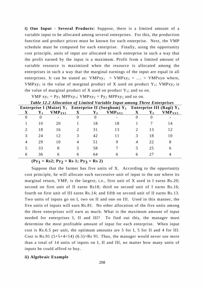
208
i) One Input - Several Products: Suppose, there is a limited amount of a variable input to be allocated among several enterprises. For this, the production function and product prices must be known for each enterprise. Next, the VMP schedule must be computed for each enterprise. Finally, using the opportunity cost principle, units of input are allocated to each enterprise in such a way that the profit earned by the input is a maximum. Profit from a limited amount of variable resource is maximized when the resource is allocated among the enterprises in such a way that the marginal earnings of the input are equal in all enterprises. It can be stated as: VMPxy1 = VMPxy2 = .... = VMPxyn where, VMPxy1 is the value of marginal product of X used on product Y1; VMPxy2 is the value of marginal product of X used on product Y2; and so on.
VMP xy1 = Py1 MPPxy1; VMPxy2 = Py2 MPPxy2 and so on. Table 12.2 Allocation of Limited Variable Input among Three Enterprises
Enterprise I (Maize) Y1 Enterprise II (Sorghum) Y2 Enterprise III (Ragi) Y3X Y1 VMPXY1 X Y2 VMPXY2 X Y3 VMPXY30 0 - 0 0 - 0 0 - 1 10 20 1 18 18 1 7 14 2 18 16 2 31 13 2 13 12 3 24 12 3 42 11 3 18 10 4 29 10 4 51 9 4 22 8 5 33 8 5 58 7 5 25 6 6 36 6 6 64 6 6 27 4
(Py1 = Rs2; Py2 = Rs 1; Py3 = Rs 2)
Suppose that the farmer has five units of X. According to the opportunity cost principle, he will allocate each successive unit of input to the use where its marginal return, VMP, is the largest; i.e., first unit of X used in I earns Rs.20; second on first unit of II earns Rs18; third on second unit of I earns Rs.16; fourth on first unit of III earns Rs.14; and fifth on second unit of II earns Rs.13. Two units of inputs go on I, two on II and one on III. Used in this manner, the five units of inputs will earn Rs.81. No other allocation of the five units among the three enterprises will earn as much. What is the maximum amount of input needed for enterprises I, II and III? To find out this, the manager must determine the most profitable amount of input for each enterprise. When input cost is Rs.6.5 per unit, the optimum amounts are 5 for I, 5 for II and 4 for III. Cost is Rs.91 (5+5+4=14) (6.5)=Rs 91. Thus, the manager would never use more than a total of 14 units of inputs on I, II and III, no matter how many units of inputs he could afford to buy.
ii) Algebraic Example

Corn response to nitrogen production function is: C=65.54+1.084NC – 0.003NC2. . .(1) Corn response to nitrogen production function is: C=65.54+1.084NC – 0.003NC2. . .(1)
Sorghum response to nitrogen function is: S = 68.07+0.830NS – 0.002 NS2 . . . . . . (2) Sorghum response to nitrogen function is: S = 68.07+0.830NS – 0.002 NS2 . . . . . . (2)
Assume that the farmer has 100 kgs of nitrogen available for 2 acres- one acre to be used for corn and one to be used for sorghum and that the price of corn is Rs.3 per kg and the price of grain sorghum is Rs2.50 per kg.
Assume that the farmer has 100 kgs of nitrogen available for 2 acres- one acre to be used for corn and one to be used for sorghum and that the price of corn is Rs.3 per kg and the price of grain sorghum is Rs2.50 per kg.
Th =Ps MPPns Th =Ps MPPns
NcNc
kglaVMVM
kglaVMVM
iiicafir
iiicafir
evbese
evbese
enen
ChCh
e allocative equations would be VMPNC =VMPNS (or) Pc MPPnce allocative equations would be VMPNC =VMPNS (or) Pc MPPnc
From (1), dC = 1.084 – 0.006 NC and from (2), dS = 0.830 – 0.004Ns d Ns dNc
VMP Nc =(1.084 – 0.006 Nc ) (3) = Rs. (3.252 – 0.018 Nc) VMP Nc =(1.084 – 0.006 Nc ) (3) = Rs. (3.252 – 0.018 Nc)
VMP Ns = (0.830 – 0.004 Ns) (2.50) =Rs. (2.075 – 0.01 Ns) VMP Ns = (0.830 – 0.004 Ns) (2.50) =Rs. (2.075 – 0.01 Ns)2.177 Nc = = 77.8 0.028
Substituting Ns = 100 – Nc, we get, 3.252 – 0.018Nc = 2.075 – 0.01 (100 – ), and Ns = 100 – 77.8 = 22.2. Substituting Ns = 100 – Nc, we get, 3.252 – 0.018Nc = 2.075 – 0.01 (100 –
), and Ns = 100 – 77.8 = 22.2.
C = 65.54 + 1.084 Nc + 0.003 Nc2 = 131.71668 x 3 = Rs.395.15 C = 65.54 + 1.084 Nc + 0.003 Nc2 = 131.71668 x 3 = Rs.395.15 S = 68.07 + 0.83 Ns – 0.002 Ns2 = 85.51o32 x 2.5 =Rs. 213.78 S = 68.07 + 0.83 Ns – 0.002 Ns2 = 85.51o32 x 2.5 =Rs. 213.78 Thus, the corn would get 77.8 kgs of nitrogen and sorghum would get 22.2
s. This allocation equates the value of marginal products and assures the rgest return from 100 kgs of nitrogen. Substituting 77.8 Kgs of nitrogen into
PNc equation and 22.2 Kgs into VMPNs equation, demonstrates that the P’s are equal to Rs.1.85.
Thus, the corn would get 77.8 kgs of nitrogen and sorghum would get 22.2 s. This allocation equates the value of marginal products and assures the
rgest return from 100 kgs of nitrogen. Substituting 77.8 Kgs of nitrogen into PNc equation and 22.2 Kgs into VMPNs equation, demonstrates that the P’s are equal to Rs.1.85.
) Two inputs - Two outputs: Consider the case in which two inputs X1 and X2 n be used to produce two products, Y1 and Y2. When the inputs are used in the st enterp g equality:
) Two inputs - Two outputs: Consider the case in which two inputs X1 and X2 n be used to produce two products, Y1 and Y2. When the inputs are used in the st enterp g equality:
Thus, t e per unit cost, en withinen reachecond ente
Thus, t e per unit cost, en withinen reachecond ente
MarginaterprisesMargina
terprises
apter 12apter 12
Py1. MPPx1y1 Py1.MPPx2y1 (or) VMPx1y1 VMPx2y1 = = Px1 Px2 Px1 Px2
rise, the equi-marginal principle dictates the followinrise, the equi-marginal principle dictates the followin
he marginal earnings of each input must be the samhe marginal earnings of each input must be the sam
a specific enterprise. When both ratios equal one, the optimum has d. The s for the use of the two inputs in the rprise.a specific enterprise. When both ratios equal one, the optimum has d. The s for the use of the two inputs in the rprise.
l returns ut must be same for both inputs in l returns ut must be same for both inputs in
: Questi: Questi
VMPx1y2 VMPx2y2 = Px1 Px2
ame condition must holdame condition must hold
per rupee spent on inp per rupee spent on inp
. Thus, the general condition is: . Thus, the general condition is: VMPx1y1 VMPx2y1 VMPx1y2 VMPx2y2 = = = Px1 Px2 Px1 Px2209
ons for Review ons for Review
1. Fill up the blanks i) Marginal rate of product substitution means the rate of change in quantity of one as a result of an unit increase in the other , given that the amount of input used remains the same. ii) An increasing rate of product transformation between two products occurs when both products are produced in the stage of returns. iii) Beyond certain level of production, both supplementary as well as complementary products become . iv) The slope of the iso revenue line is determined by the . v) When the input is scarce, it is allocated to each enterprise in such a way that the profit earned by the input is . vi) At maximum revenue yielding combination of outputs, the slope of production possibility curve is equal to the slope of . vii) Complementary occurs when one of the products produces an used by the other product. viii) In case of complementary products the value of MRPS will be . 2. Define the following: i) Production possibility curve. ii) Iso revenue line. iii) Marginal Rate of Product Transformation. 3. Write short notes or short answers on the following: i) Distinguish between Iso product curve and Iso resource curve. ii) Law of equi marginal returns. iii) Output expansion path. 4. Answer the following: i) Explain the maximum revenue yielding combination of outputs with
illustration. ii) Explain the different types of relationships between products.
A. CLASS
Farminproducts, cfunctioningproducts oproductionfunctioningorganizatiowith questpooled or
TYPES AND SYSTEMS OF FARMING
IFICATION OF FARMING
g may be classified on the basis of similarity in i) combinations of rop and livestock raised and ii) the mode of economic and social - private, co-operative, state or collective, etc. The combinations of n a given farm and the methods or practices that are used in the of these products based on the ways of economic and social in farming are known as system of farming. It is concerned with the nal set up under which the farm is being run. Systems mainly deal ions like who is the owner of the land, whether the resources are used individually, and who makes the managerial decisions. It is
210
211
classified into five groups, namely, peasant, co-operative, state, capitalistic and collective farming. When farms in a group are quite similar in the kinds and productions of the crops and livestock that are produced and the methods and practices followed in production, the group is described as type of farming. It includes specialized, diversified, mixed and ranching.
i) Type of Farming
a) Specialized Farm: Specialization means that the farmers specialize in one enterprise such as crop, dairying, poultry or tea estate, etc.
1) Advantages of specialized farming
i) Better use of land: It is more profitable to grow a crop on a land best suited to it. E.g.) Jute cultivation on a swampy land.
ii) Better Marketing: Specialization allows for better assembling, grading, processing, storing, transporting and financing of the produce.
iii) Better Management: As there are fewer enterprises, wastage can easily be detected and they can be better managed.
iv) Less equipment and labour are needed.
v) Costly and efficient machinery can be used. vi) Efficiency and skills are increased: Specialization allows a man to be more efficient and expert at doing a few things.
2) Disadvantages of specialized farming
i) There is a greater risk - failure of crop and market together may ruin the farmer.
ii) Productive resources – land, labour and capital are not fully utilized.
iii) Fertility of soil cannot be properly maintained due to lack of suitable rotations.
iv) By products of the farm cannot be fully utilized due to lack of sufficient livestock on the farm.
v) Farm returns in cash are not generally received more than once in a year, i.e., there is no regular farm return.
b) Diversified Farming
212
A Farm on which no single or source of income yields 50 per cent of the total receipt is called a diversified farm. More number of enterprises are taken up on the farm and no single enterprise is relatively much more important.
1) Advantages of diversified farming
i) Better use of land, labour and capital: Better use of land through adoption of crop rotations, steady employment generation and more efficient use of equipment are obtained.
ii) Business risk is reduced due to a crop failure or unfavourable market prices.
iii) Regular and quicker returns are obtained from various enterprises.
2) Disadvantages of diversified farming.
i) Because of varied jobs in diversified farming, a farmer can efficiently supervise only limited number of workers.
ii) Better equipping of the farm is not possible because it is not economical to have extensive implements and machinery for each enterprise.
c) Mixed Farming
Mixed farming is a type of farming under which crop production is combined with livestock rearing. The livestock enterprise is complementary to crop production programme so as to provide a balanced and productive system of farming. In mixed farming, the contribution of livestock activities to gross farm income should be a minimum of 10 per cent and a maximum of 49 per cent.
1) Advantage of Mixed Farming
i) Mixed farming helps in the maintenance of soil fertility. By products of crop production, namely, green and dry fodder, rice bran, gram husk and so on are better used for live stock. On the other hand, farm yard manure enriches the soil with important nutrients.
ii) Draught animals are used in crop production and transport.
iii) It provides regular income and employment.
d) Ranching
A ranch differs from other type of crop and livestock farming in that the livestock graze the natural vegetation. Ranch land is not utilized by tilling or
213
raising crops. The ranchers have no land of their own and make use of the public grazing land. Ranching is followed in Australia, America, Tibet and certain parts of India (Bikaner in Rajesthan).
e) Determinants of Type of Farming
The type of farming is determined by 1) Physical, 2) Economic and 3) Social factors.
1) Physical Factors: The physical factors namely climate, soil and topography have influence in determining the type of farming.
2) Economic Factors: Marketing cost, changes in input and output prices, availability of resources like land, labour and capital, competition between enterprises, miscellaneous factors such as personal likes and dislikes, prevalence of pest and diseases, etc. influence type of farming.
3) Social Factors: The kind of people in the community and the provision of protection of crops against the hazards of bird and animal ravages may influence the farming community to change the pattern of cropping. The co-operative spirit in providing security to crops, benefits resulting from low transport costs through collective sale and better marketing facilities permit farmers to expand some enterprises like fruit farming, dairying or poultry rearing.
ii) System of Farming
System of farming is generally referred to the method of agriculture and the type of ownership to land. The system of farming is comprised of i) co operative farming, ii) collective farming, iii) capitalistic farming, iv) state farming and v) peasant farming.
i) Co-operative Farming
Co-operative farming means a system under which all agricultural operations or part of them are carried on jointly by the farmers on a voluntary basis in order to exploit modern cultivation practices and economies of scale. Co-operative farming societies have four different forms:
a) Forms of co-operative Farming: There are four different forms of co-operative farming. They are: Co-operative Better farming, Co-operative Joint farming, Co-operative Tenant farming and Co-operative Collective farming.
214
1) Under the system of co-operative better farming, the land is not pooled and cultivation is carried on by each farmer separately. The co-operative better farming society promotes the interest of the members through the adoption of better farming practices. It arranges for the purchase of seeds, manure, joint use of machinery etc. A member is free to follow his own way of farming except in respect of the purpose for which he joins the society, e.g. irrigation, purchase of seeds or marketing of produce, etc.
2) In co-operative joint farming, the land of the members is pooled for joint cultivation. The ownership of each member over his own land is recognized by payment of a divided in proportion to the value of his land. Members work on the land under the direction of managing committee and each member receives wages for his daily labour.
3) Under the system of co-operative tenant farming, the land is held by the society and not by the members individually. The land is divided into plots which are leased out for cultivation to individual members. The society also arranges for inputs like credit, seeds and manure besides arranging for marketing of the produce. Each member pays rent of his plot to the society.
4) In co-operative collective farming, the land is owned by the society and cultivation is done jointly. The method of work of the society is similar to that of co-operative joint farming society. But the right or share of individual members in the land is not recognized by the co-operative collective farming societies and hence, they have no appeal to the farmers due to their strong attachment to the ownership of land.
ii) Collective Farming
In collective farming, the members surrender their land, livestock and dead stock to the society. The members work together under a management committee elected by them. The committee allocates work to members, distributes income and market surpluses and puts all members into labour to see that the work is done. The main source of income is through labour earnings.
iii) Capitalistic Farming
The capitalistic farming is based on capitalistic methods where land lordism exists as in America or England. The role of capital is more; wage (hired) labour is more than family labour under this farming. In India, this type of farming can be seen in commercialized agricultural areas where farm production is market
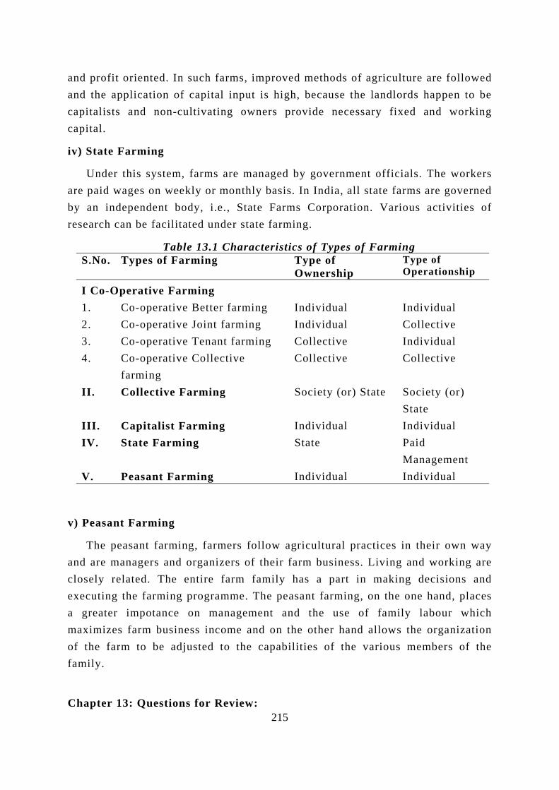
215
and profit oriented. In such farms, improved methods of agriculture are followed and the application of capital input is high, because the landlords happen to be capitalists and non-cultivating owners provide necessary fixed and working capital.
iv) State Farming
Under this system, farms are managed by government officials. The workers are paid wages on weekly or monthly basis. In India, all state farms are governed by an independent body, i.e., State Farms Corporation. Various activities of research can be facilitated under state farming.
Table 13.1 Characteristics of Types of Farming S.No. Types of Farming Type of
Ownership Type of Operationship
I Co-Operative Farming 1. Co-operative Better farming Individual Individual 2. Co-operative Joint farming Individual Collective 3. Co-operative Tenant farming Collective Individual 4. Co-operative Collective
farming Collective Collective
II. Collective Farming Society (or) State Society (or) State
III. Capitalist Farming Individual Individual IV. State Farming State Paid
Management V. Peasant Farming Individual Individual
v) Peasant Farming
The peasant farming, farmers follow agricultural practices in their own way and are managers and organizers of their farm business. Living and working are closely related. The entire farm family has a part in making decisions and executing the farming programme. The peasant farming, on the one hand, places a greater impotance on management and the use of family labour which maximizes farm business income and on the other hand allows the organization of the farm to be adjusted to the capabilities of the various members of the family.
Chapter 13: Questions for Review:
1. Fill up the Blanks i) The contribution of income from livestock enterprise to gross farm income ranges from per cent to per cent. ii) In Co-operative better farming, the type of ownership and operatorship are
and respectively. iii) In ranching, the farmers have their own land for grazing the animals. iv) In Mixed farming, crop and livestock production are to each other. v) In farming, the risk is minimized.
2. Define the following: i) Systems of farming and Types of farming. ii) Capitalistic farming. iii) Peasant farming. iv) Ranching. v) Mixed farming.
3. Distinguish between the following: i) Co-operative Collective Farming and Collective Farming. ii) Collective farming and State farming. iii) Specialization and Diversification. iv) Co-operative tenant farming and Co-operative better farming. v) Capitalistic farming and Collective farming. vi) Ranching and Mixed farming.
4. Answer the following: i) Explain the functioning of different types of co-operative farming. ii) Explain the factors influencing the type of farming. iii) Explain the advantages and disadvantages of different types of farming.
216
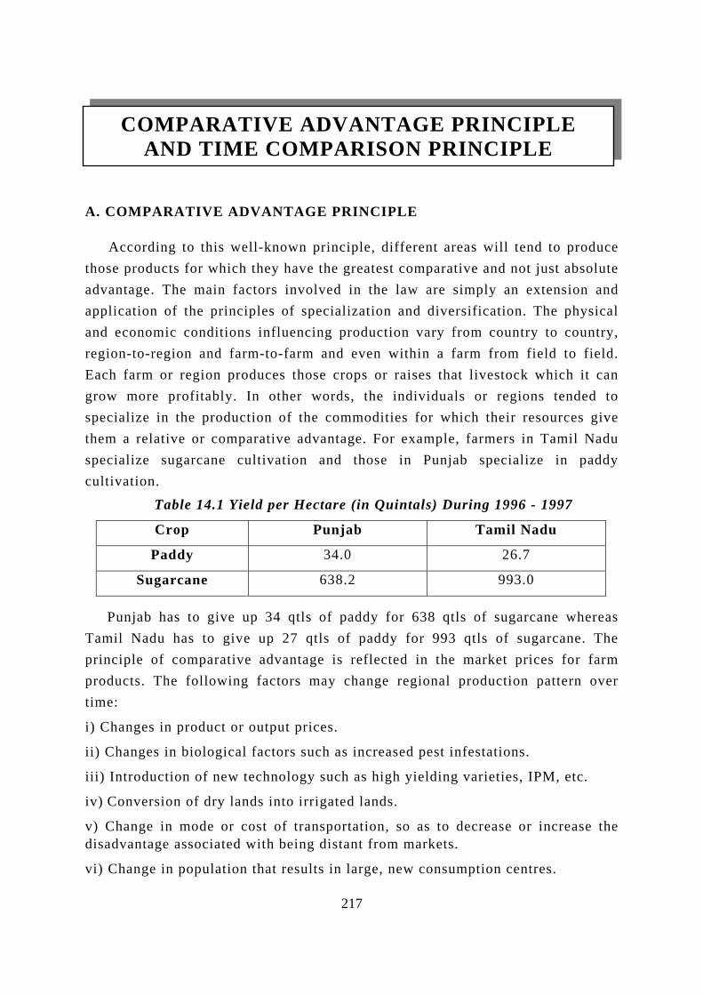
A. C
Athoseadvaappliand regioEachgrowspecthemspecculti
PTamprincprodtime
i) Ch
ii) C
iii) I
iv) C
v) Cdisad
vi) C
COMPARATIVE ADVANTAGE PRINCIPLE
AND TIME COMPARISON PRINCIPLE
OMPARATIVE ADVANTAGE PRINCIPLE
ccording to this well-known principle, different areas will tend to produce products for which they have the greatest comparative and not just absolute
ntage. The main factors involved in the law are simply an extension and cation of the principles of specialization and diversification. The physical economic conditions influencing production vary from country to country, n-to-region and farm-to-farm and even within a farm from field to field. farm or region produces those crops or raises that livestock which it can more profitably. In other words, the individuals or regions tended to
ialize in the production of the commodities for which their resources give a relative or comparative advantage. For example, farmers in Tamil Nadu ialize sugarcane cultivation and those in Punjab specialize in paddy vation.
Table 14.1 Yield per Hectare (in Quintals) During 1996 - 1997
Crop Punjab Tamil Nadu
Paddy 34.0 26.7
Sugarcane 638.2 993.0
unjab has to give up 34 qtls of paddy for 638 qtls of sugarcane whereas il Nadu has to give up 27 qtls of paddy for 993 qtls of sugarcane. The iple of comparative advantage is reflected in the market prices for farm
ucts. The following factors may change regional production pattern over :
anges in product or output prices.
hanges in biological factors such as increased pest infestations.
ntroduction of new technology such as high yielding varieties, IPM, etc.
onversion of dry lands into irrigated lands.
hange in mode or cost of transportation, so as to decrease or increase the vantage associated with being distant from markets.
hange in population that results in large, new consumption centres.
217
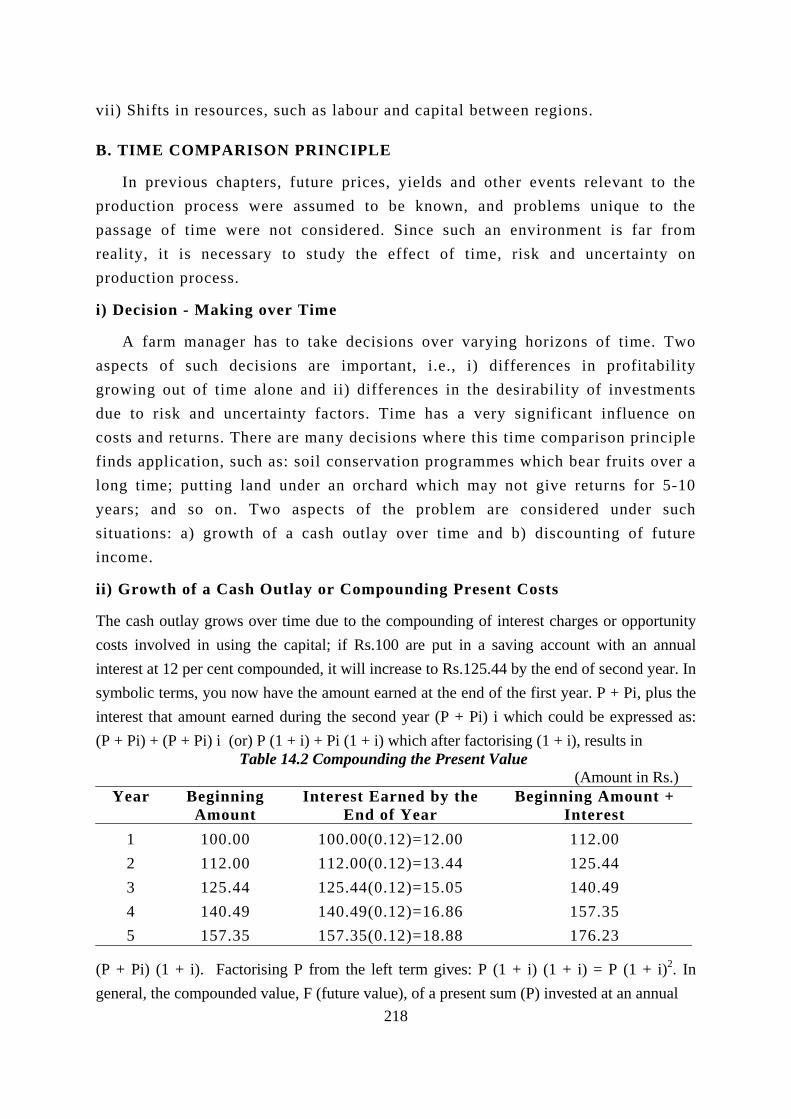
218
vii) Shifts in resources, such as labour and capital between regions.
B. TIME COMPARISON PRINCIPLE
In previous chapters, future prices, yields and other events relevant to the production process were assumed to be known, and problems unique to the passage of time were not considered. Since such an environment is far from reality, it is necessary to study the effect of time, risk and uncertainty on production process.
i) Decision - Making over Time
A farm manager has to take decisions over varying horizons of time. Two aspects of such decisions are important, i.e., i) differences in profitability growing out of time alone and ii) differences in the desirability of investments due to risk and uncertainty factors. Time has a very significant influence on costs and returns. There are many decisions where this time comparison principle finds application, such as: soil conservation programmes which bear fruits over a long time; putting land under an orchard which may not give returns for 5-10 years; and so on. Two aspects of the problem are considered under such situations: a) growth of a cash outlay over time and b) discounting of future income.
ii) Growth of a Cash Outlay or Compounding Present Costs
The cash outlay grows over time due to the compounding of interest charges or opportunity costs involved in using the capital; if Rs.100 are put in a saving account with an annual interest at 12 per cent compounded, it will increase to Rs.125.44 by the end of second year. In symbolic terms, you now have the amount earned at the end of the first year. P + Pi, plus the interest that amount earned during the second year (P + Pi) i which could be expressed as: (P + Pi) + (P + Pi) i (or) P (1 + i) + Pi (1 + i) which after factorising (1 + i), results in
Table 14.2 Compounding the Present Value (Amount in Rs.)
Year Beginning Amount
Interest Earned by the End of Year
Beginning Amount + Interest
1 100.00 100.00(0.12)=12.00 112.00 2 112.00 112.00(0.12)=13.44 125.44 3 125.44 125.44(0.12)=15.05 140.49 4 140.49 140.49(0.12)=16.86 157.35 5 157.35 157.35(0.12)=18.88 176.23
(P + Pi) (1 + i). Factorising P from the left term gives: P (1 + i) (1 + i) = P (1 + i)2. In general, the compounded value, F (future value), of a present sum (P) invested at an annual
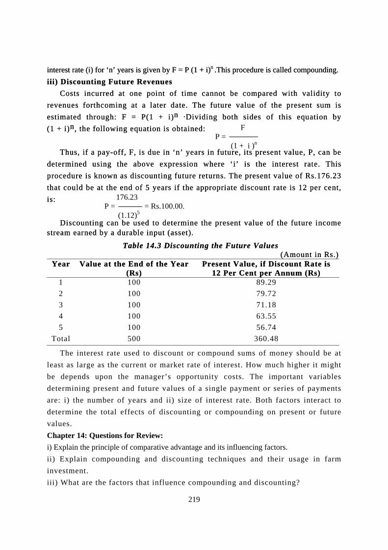
interest rate (i) for ‘n’ years is given by F = P (1 + i)n .This procedure is called compounding. interest rate (i) for ‘n’ years is given by F = P (1 + i)n .This procedure is called compounding.
iii) Discounting Future Revenues iii) Discounting Future Revenues
219
F P = (1 + .i )n
Costs incurred at one point of time cannot be compared with validity to revenues forthcoming at a later date. The future value of the present sum is estimated through: F = P(1 + i)n .Dividing both sides of this equation by (1 + i)n, the following equation is obtained:
Costs incurred at one point of time cannot be compared with validity to revenues forthcoming at a later date. The future value of the present sum is estimated through: F = P(1 + i)n .Dividing both sides of this equation by (1 + i)n, the following equation is obtained:
176.23 P = = Rs.100.00. (1.12)5
Thus, if a pay-off, F, is due in ‘n’ years in future, its present value, P, can be determined using the above expression where ‘i’ is the interest rate. This procedure is known as discounting future returns. The present value of Rs.176.23 that could be at the end of 5 years if the appropriate discount rate is 12 per cent, is:
Thus, if a pay-off, F, is due in ‘n’ years in future, its present value, P, can be determined using the above expression where ‘i’ is the interest rate. This procedure is known as discounting future returns. The present value of Rs.176.23 that could be at the end of 5 years if the appropriate discount rate is 12 per cent, is:
Discounting can be used to determine the present value of the future income stream earned by a durable input (asset).
Discounting can be used to determine the present value of the future income stream earned by a durable input (asset).
Table 14.3 Discounting the Future Values Table 14.3 Discounting the Future Values (Amount in Rs.) (Amount in Rs.) Year Year Value at the End of the Year Value at the End of the Year
(Rs) (Rs) Present Value, if Discount Rate is
12 Per Cent per Annum (Rs) Present Value, if Discount Rate is
12 Per Cent per Annum (Rs) 1 100 89.29 2 100 79.72 3 100 71.18 4 100 63.55 5 100 56.74
Total 500 360.48
The interest rate used to discount or compound sums of money should be at least as large as the current or market rate of interest. How much higher it might be depends upon the manager’s opportunity costs. The important variables determining present and future values of a single payment or series of payments are: i) the number of years and ii) size of interest rate. Both factors interact to determine the total effects of discounting or compounding on present or future values. Chapter 14: Questions for Review: i) Explain the principle of comparative advantage and its influencing factors. ii) Explain compounding and discounting techniques and their usage in farm investment. iii) What are the factors that influence compounding and discounting?
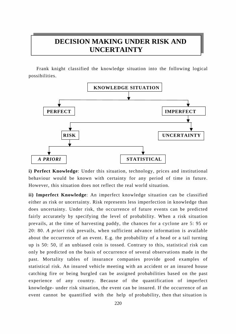
220
DECISION MAKING UNDER RISK AND UNCERTAINTY
Frank knight classified the knowledge situation into the following logical possibilities.
KNOWLEDGE SITUATION
PERFECT IMPERFECT
RISK UNCERTAINTY
A PRIORI STATISTICAL
i) Perfect Knowledge: Under this situation, technology, prices and institutional behaviour would be known with certainty for any period of time in future. However, this situation does not reflect the real world situation.
ii) Imperfect Knowledge: An imperfect knowledge situation can be classified either as risk or uncertainty. Risk represents less imperfection in knowledge than does uncertainty. Under risk, the occurrence of future events can be predicted fairly accurately by specifying the level of probability. When a risk situation prevails, at the time of harvesting paddy, the chances for a cyclone are 5: 95 or 20: 80. A priori risk prevails, when sufficient advance information is available about the occurrence of an event. E.g. the probability of a head or a tail turning up is 50: 50, if an unbiased coin is tossed. Contrary to this, statistical risk can only be predicted on the basis of occurrence of several observations made in the past. Mortality tables of insurance companies provide good examples of statistical risk. An insured vehicle meeting with an accident or an insured house catching fire or being burgled can be assigned probabilities based on the past experience of any country. Because of the quantification of imperfect knowledge- under risk situation, the event can be insured. If the occurrence of an event cannot be quantified with the help of probability, then that situation is
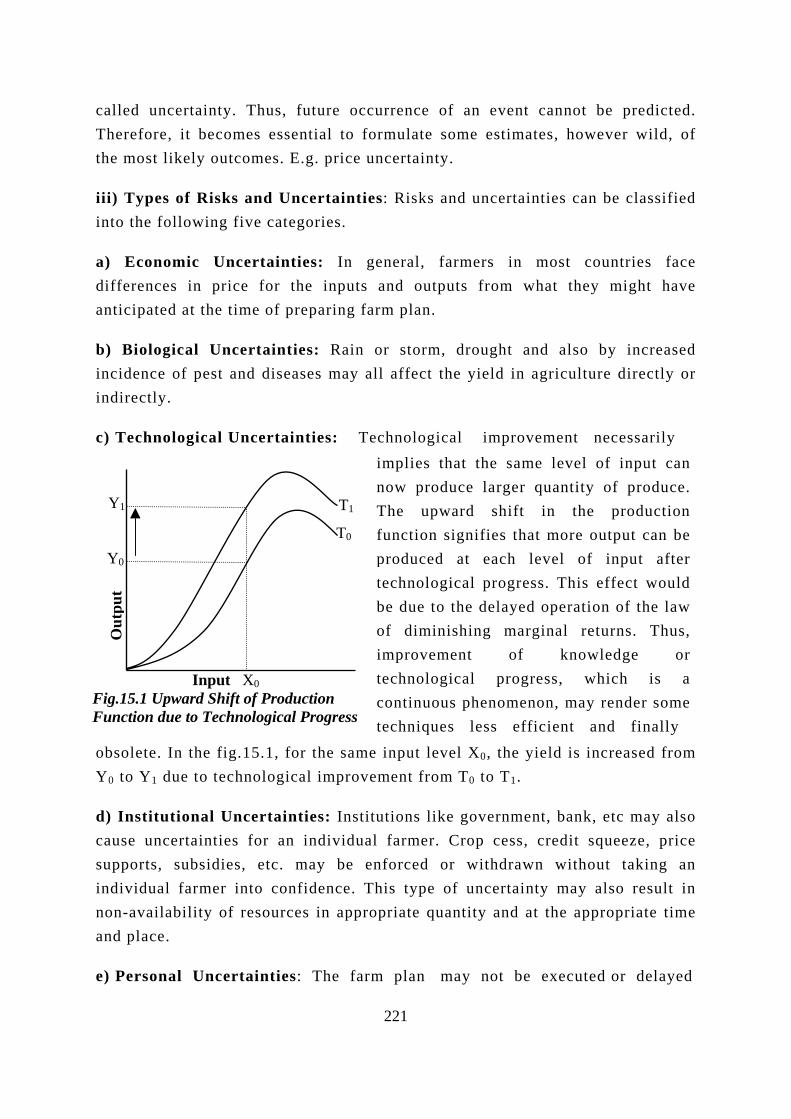
called uncertainty. Thus, future occurrence of an event cannot be predicted. Therefore, it becomes essential to formulate some estimates, however wild, of the most likely outcomes. E.g. price uncertainty.
iii) Types of Risks and Uncertainties: Risks and uncertainties can be classified into the following five categories.
a) Economic Uncertainties: In general, farmers in most countries face differences in price for the inputs and outputs from what they might have anticipated at the time of preparing farm plan.
b) Biological Uncertainties: Rain or storm, drought and also by increased incidence of pest and diseases may all affect the yield in agriculture directly or indirectly.
1
c) Technological Uncertainties: T
oY
dcsina
e
Y
0
0
YOut
put
bsolete. In the fig.15.1, for the0 to Y1 due to technological im
) Institutional Uncertainties:ause uncertainties for an indiupports, subsidies, etc. may ndividual farmer into confidenon-availability of resources innd place.
) Personal Uncertainties: Th
T1
T
Input X0Fig.15.1 Upward Shift of Production Function due to Technological Progress
samprov
Instividuabe ece. T
appr
e far
echnological improvement necessarily implies that the same level of input cannow produce larger quantity of produce.The upward shift in the productionfunction signifies that more output can beproduced at each level of input aftertechnological progress. This effect wouldbe due to the delayed operation of the lawof diminishing marginal returns. Thus,improvement of knowledge ortechnological progress, which is acontinuous phenomenon, may render sometechniques less efficient and finally
221
e input level X0, the yield is increased from ement from T0 to T1.
tutions like government, bank, etc may also l farmer. Crop cess, credit squeeze, price nforced or withdrawn without taking an his type of uncertainty may also result in
opriate quantity and at the appropriate time
m plan may not be executed or delayed
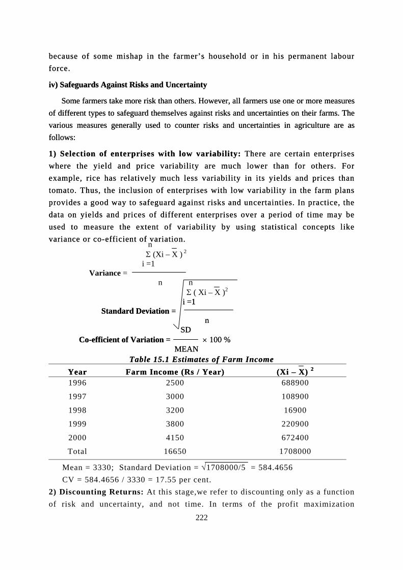
because of some mishap in the farmer’s household or in his permanent labour force. because of some mishap in the farmer’s household or in his permanent labour force.
iv) Safeguards Against Risks and Uncertainty iv) Safeguards Against Risks and Uncertainty
Some farmers take more risk than others. However, all farmers use one or more measures of different types to safeguard themselves against risks and uncertainties on their farms. The various measures generally used to counter risks and uncertainties in agriculture are as follows:
Some farmers take more risk than others. However, all farmers use one or more measures of different types to safeguard themselves against risks and uncertainties on their farms. The various measures generally used to counter risks and uncertainties in agriculture are as follows:
222
n or co-efficient of v
Σ (Xi – X ) 2. i =1 Variance = .n n Σ ( Xi – X ) 2
. i =1 i =1 Standard Deviation =
Standard Deviation = n . n . SD SD Co-efficient of Variation = × 100 % Co-efficient of Variation = × 100 % MEAN MEAN
1) Selection of enterprises with low variability: There are certain enterprises where the yield and price variability are much lower than for others. For example, rice has relatively much less variability in its yields and prices than tomato. Thus, the inclusion of enterprises with low variability in the farm plans provides a good way to safeguard against risks and uncertainties. In practice, the data on yields and prices of different enterprises over a period of time may be used to measure the extent of variability by using statistical concepts like variance ariation.
1) Selection of enterprises with low variability: There are certain enterprises where the yield and price variability are much lower than for others. For example, rice has relatively much less variability in its yields and prices than tomato. Thus, the inclusion of enterprises with low variability in the farm plans provides a good way to safeguard against risks and uncertainties. In practice, the data on yields and prices of different enterprises over a period of time may be used to measure the extent of variability by using statistical concepts like variance or co-efficient of variation.
Table 15.1 Estimates of Farm Income Table 15.1 Estimates of Farm Income
Year Year Farm Income (Rs / Year) Farm Income (Rs / Year) (Xi – X) 2(Xi – X) 2
1996 2500 688900
1997 3000 108900
1998 3200 16900
1999 3800 220900
2000 4150 672400
Total 16650 1708000
Mean = 3330; Standard Deviation = √1708000/5 = 584.4656 CV = 584.4656 / 3330 = 17.55 per cent.
2) Discounting Returns: At this stage,we refer to discounting only as a function of risk and uncertainty, and not time. In terms of the profit maximization

223
condition of VMP = Px, discounting means that either the output price (Py) is decreased or input price (Px) is increased by some proportion or it can be of both. Thus, the profit maximization level of the variable input X1 may now be lower with discounting than otherwise.
3) Insurance: Insurance covers the cost to some extent so as to minimize the loss.
4) Forward Contracts: They reduce the future prices of both inputs and outputs into certainty. Pre-harvest contracts of mango, share cropping, i.e., forward contract in kind are some examples for this.
5) Flexibility: This refers to the convenience with which the organization of production on a farm can be changed.
a) Time Flexibility: Time flexibility may be introduced either through proper selection of products or production methods or partly by both. Orchard plantation is a relatively rigid enterprise than annual crops. A short-lived farm structure is more flexible that the durable.
b) Cost flexibility: Wherever time flexibility is of limited use, cost flexibility becomes important. Cost flexibility refers to variations in output within the structure of a plant of a longer life. Extension or concentration of output, whenever desired by favourable prices or yields can be brought about at lower cost for a given farm (plant). Owning rather than custom hiring a power tiller may have more cost flexibility.
c) Product flexibility: Product flexibility aims at changes in production in response to price changes. In this category, machines, farm structure, etc, can be readily shifted from one product to another.
6) Liquidity: This refers to the case with which assets in a farm can be converted into cash, the most “liquid” of all assets. If some of the assets are held in the form, which can be easily converted, into cash, it provides a safeguard to the farmer by enabling him to make necessary adjustments in response to risks and uncertainties of various types.
7) Diversification: It is a means of stabilizing incomes rather than profit maximizing technique relating to receive benefits of complementarity or supplementarity. Under risky environment, a farmer may not specialize in a single enterprise over a period of time even if substitution and price ratios may so dictate as discussed under product-product relationship. Instead, he may
choose several enterprises in some proportion overtime, so as to distribute the risk factor. Like flexibility, it has no provision to reap large gains due to high prices or yields over time, but serves as a good method to prevent heavy losses. However, the diversification of farm activities may deprive the entrepreneur of all the advantages of specialization.
8) Maintenance of resources in reserve: Many a time, there is a risk or uncertainty about the availability of the right inputs, in the required quantity at the right time and place and at a reasonable price. This may be due to the imbalance between demand and supply of the resources. To overcome this problem, the best way is to maintain sufficient stocks of such inputs. Maintenance of sufficient stocks depends on the availability of funds, his ability to fore cast prices and the availability of resources and storage facilities in the farm.
9) Adjustment to uncertain of Inputs: When a resource is not available, the best way the farmer can safeguard against such risk and uncertainty is by exploring the use of some other resource as a substitute. If a farmer is uncertain about the availability of inputs, he would do better by choosing the best alternatives, i.e., sowing the second best variety, using the second best fertilizer, using the second best method of harvesting etc. Chapter 15: Questions for Review: 1. Fill up the blanks. i) If the occurrence of an event cannot be quantified with the help of probability, then that situation is called ; while the occurrence of an event can be quantified with the help of probability, in case of . ii) Inclusion of enterprises with low variability in the farm plans reduces . iii) Diversification is a means of stabilizing rather than profit maximizing technique. 2.Define the following: i) Risk and Uncertainty. ii) Forward contract. 3.Write short notes i) Perfect knowledge and imperfect knowledge situations ii) Technological uncertainty iii) Flexibility. iv) Diversification of enterprise as a measure of reducing risk 2. Answer the following: i) Explain the different types of uncertainties with suitable examples. ii) Explain the different measures to safeguard against risk and uncertainty.
224
A. FARM BUSIN
Efficient manaany point of timegoing on. This heobjectives of farm
i) to evaluate
ii) to identify
iii) to remove
iv) to prepareso as to acquire c
i) Steps or Stages
a) Proper reco
b) Analysis of
c) Interpretati
a. Recording ofaspects of the farsound knowledge
b. Analysis of dsheet and income efficiency.
c. Interpretationperformance of interpretation of the business.
ii) Advantages of
a) They are the m
FARM BUSINESS ANALYSIS
ESS AND CONTROL
gers want to be able to determine the position of a business at . They also want a basis for evaluating where the business is lps their control of the business operations overtime. Thus, the business at a particular point of time are:
the performance of the business at a particular point of time;
the weakness of the business;
the hurdles and improve the business; and
financial documents like balance sheet and income statement redit, design farm policies and prepare tax statement.
of Farm Business Analysis
rding of accounts and activities.
the data.
on of the results.
data: A systematic recording of information on financial m is essential for farm business analysis and for this purpose, a on book keeping and accounting is essential.
ata: The data collected would be useful to construct balance statement. Financial ratio analysis would also increase the farm
of the results: The financial analysis would indicate the the business and suggest measures for improvement. The results would be more useful to understand the performance of
Farm Records and Accounts
eans to increase the farm income.
225
226
b) They are the basis for diagnosis and planning.
c) They show the ways to improve the managerial ability of the farmer.
d) They are useful for credit acquisition and management.
e) They provide database for conducting research in agricultural economics.
f) They form the basis for designing government policies - land policy, price policy, national farm policies, etc.
iii) Problems in Farm Accounting
a) As Indian farmers carry out only subsistence nature of farming, recording is not essential to them.
b) Indian farmer acts as an owner, manager and labourer. Hence, recording becomes complex.
c) Illiteracy and lack of business awareness of farmers prohibit them to have farm records.
d) Fear of taxation prevents farmers from recording and accounting the information.
e) Forecasting becomes complicated because of very high risk and uncertainties involved in farming.
iv) Types of Farm Records: Farm records can be classified into three categories, i.e., inventories, production records and financial records.
a) Inventory: Farm inventory includes a complete listing of all that a farm owns and owes at a particular date, generally at the beginning and the end of each agricultural year. It includes not only the listing of physical assets but also assigning values of all such assets, liabilities and debts as well. There are two steps involved in taking a farm inventory.
1) Examination of Physical Assets: It includes a complete listing of all the physical assets including a verification of weights and measurements. The losses, wastages, shrinkages or gains, which accrue over time, are all accounted for.
2) Valuation of Physical Assets: A few common methods of valuation are discussed below:
i) Valuation at Cost: The amount of money actually invested on the asset when
it was acquired is entered in the inventory. This method has the following limitations: a) it cannot be used for the valuation of farm products; b) the effects of inflation and deflation are ignored; and c) original investment value has only a limited use, when valuation is taken up somewhere in the middle of the business.
ii) Cost or market prices whichever is lower: This is used for valuing the purchased farm supplies.
iii) Net Selling Price: It represents market price less the selling costs. For all assets that will be sold within the year, the net selling price is used. Crops or livestock produced for the market can be valued with this method.
iv) Cost Less Depreciation: The value of asset in subsequent years can be estimated by subtracting the depreciation from its cost. Machinery, breeding livestock and buildings constructed recently can be evaluated with this method. But this method cannot be applied for products produced from the farm.
v) Replacement Cost: It represents a value of an asset, which is equal to the cost needed to reproduce the asset at the present prices and under the existing technological improvements. This method may be successfully employed for the valuation of fixed and long-lived assets.
vi) Replacement Cost less Depreciation: It represents an improvement over the previous method as it provides a more realistic valuation of fixed and long-lived assets like buildings, particularly, when wide price changes occur. However, this method should be used very carefully as it may often lead to over valuation.
vii) Income Capitalization: For assets like land whose contribution towards the income can be measured for each production period and which has long life, income capitalization is an ideal method of valuation. If a certain piece of land is expected to give an uniform income of Rs.1,000 per year indefinitely and the rate of interest is 10 per cent per annum, the present value of the land, then, can be easily assessed by using this method, i.e.,
Return per Year ( R ) 1,000 Present Value (PV) = = = Rs. 10,000 Interest Rate per Annum ( r ) 0.10
227
Thus, the piece of land in question would be valued at Rs.10,000.
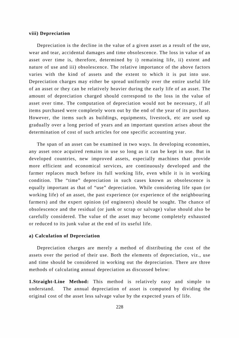
228
viii) Depreciation
Depreciation is the decline in the value of a given asset as a result of the use, wear and tear, accidental damages and time obsolescence. The loss in value of an asset over time is, therefore, determined by i) remaining life, ii) extent and nature of use and iii) obsolescence. The relative importance of the above factors varies with the kind of assets and the extent to which it is put into use. Depreciation charges may either be spread uniformly over the entire useful life of an asset or they can be relatively heavier during the early life of an asset. The amount of depreciation charged should correspond to the loss in the value of asset over time. The computation of depreciation would not be necessary, if all items purchased were completely worn out by the end of the year of its purchase. However, the items such as buildings, equipments, livestock, etc are used up gradually over a long period of years and an important question arises about the determination of cost of such articles for one specific accounting year.
The span of an asset can be examined in two ways. In developing economies, any asset once acquired remains in use so long as it can be kept in use. But in developed countries, new improved assets, especially machines that provide more efficient and economical services, are continuously developed and the farmer replaces much before its full working life, even while it is in working condition. The “time” depreciation in such cases known as obsolescence is equally important as that of “use” depreciation. While considering life span (or working life) of an asset, the past experience (or experience of the neighbouring farmers) and the expert opinion (of engineers) should be sought. The chance of obsolescence and the residual (or junk or scrap or salvage) value should also be carefully considered. The value of the asset may become completely exhausted or reduced to its junk value at the end of its useful life.
a) Calculation of Depreciation
Depreciation charges are merely a method of distributing the cost of the assets over the period of their use. Both the elements of depreciation, viz., use and time should be considered in working out the depreciation. There are three methods of calculating annual depreciation as discussed below:
1.Straight-Line Method: This method is relatively easy and simple to understand. The annual depreciation of asset is computed by dividing the original cost of the asset less salvage value by the expected years of life.
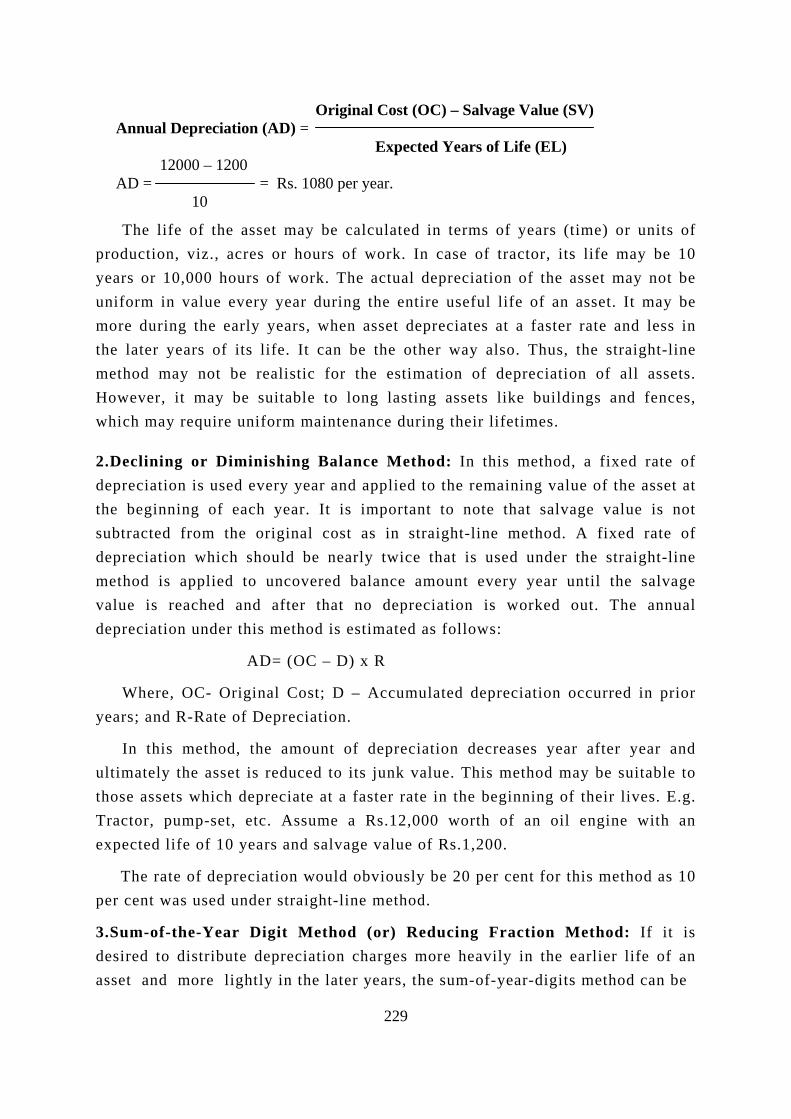
pryeunmthmHw
2.dethsudemvade
ye
ulthTrex
pe
3.deas
Original Cost (OC) – Salvage Value (SV) Annual Depreciation (AD) = Expected Years of Life (EL) 12000 – 1200 AD = = Rs. 1080 per year. 10
229
The life of the asset may be calculated in terms of years (time) or units of oduction, viz., acres or hours of work. In case of tractor, its life may be 10 ars or 10,000 hours of work. The actual depreciation of the asset may not be iform in value every year during the entire useful life of an asset. It may be
ore during the early years, when asset depreciates at a faster rate and less in e later years of its life. It can be the other way also. Thus, the straight-line ethod may not be realistic for the estimation of depreciation of all assets. owever, it may be suitable to long lasting assets like buildings and fences, hich may require uniform maintenance during their lifetimes.
Declining or Diminishing Balance Method: In this method, a fixed rate of preciation is used every year and applied to the remaining value of the asset at e beginning of each year. It is important to note that salvage value is not btracted from the original cost as in straight-line method. A fixed rate of preciation which should be nearly twice that is used under the straight-line ethod is applied to uncovered balance amount every year until the salvage lue is reached and after that no depreciation is worked out. The annual preciation under this method is estimated as follows:
AD= (OC – D) x R
Where, OC- Original Cost; D – Accumulated depreciation occurred in prior ars; and R-Rate of Depreciation.
In this method, the amount of depreciation decreases year after year and timately the asset is reduced to its junk value. This method may be suitable to ose assets which depreciate at a faster rate in the beginning of their lives. E.g. actor, pump-set, etc. Assume a Rs.12,000 worth of an oil engine with an pected life of 10 years and salvage value of Rs.1,200.
The rate of depreciation would obviously be 20 per cent for this method as 10 r cent was used under straight-line method.
Sum-of-the-Year Digit Method (or) Reducing Fraction Method: If it is sired to distribute depreciation charges more heavily in the earlier life of an set and more lightly in the later years, the sum-of-year-digits method can be
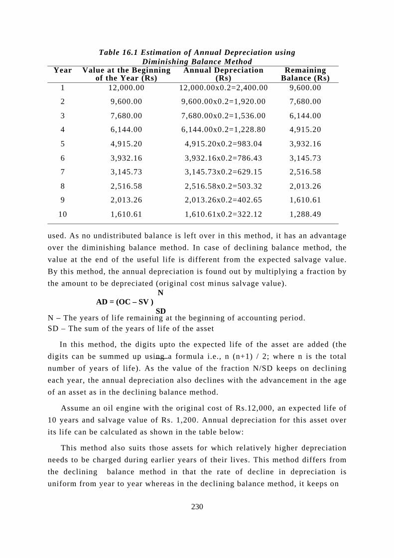
Table 16.1 Estimation of Annual Depreciation using Diminishing Balance Method
Year Value at the Beginning of the Year (Rs)
Annual Depreciation (Rs)
Remaining Balance (Rs)
1 12,000.00 12,000.00x0.2=2,400.00 9,600.00
2 9,600.00 9,600.00x0.2=1,920.00 7,680.00
3 7,680.00 7,680.00x0.2=1,536.00 6,144.00
4 6,144.00 6,144.00x0.2=1,228.80 4,915.20
5 4,915.20 4,915.20x0.2=983.04 3,932.16
6 3,932.16 3,932.16x0.2=786.43 3,145.73
7 3,145.73 3,145.73x0.2=629.15 2,516.58
8 2,516.58 2,516.58x0.2=503.32 2,013.26
9 2,013.26 2,013.26x0.2=402.65 1,610.61
10 1,610.61 1,610.61x0.2=322.12 1,288.49
230
N
used. As no undistributed balance is left over in this method, it has an advantage over the diminishing balance method. In case of declining balance method, the value at the end of the useful life is different from the expected salvage value. By this method, the annual depreciation is found out by multiplying a fraction by the amount to be depreciated (original cost minus salvage value).
AD = (OC – SV ) SD
N – The years of life remaining at the beginning of accounting period. SD – The sum of the years of life of the asset
In this method, the digits upto the expected life of the asset are added (the digits can be summed up using a formula i.e., n (n+1) / 2; where n is the total number of years of life). As the value of the fraction N/SD keeps on declining each year, the annual depreciation also declines with the advancement in the age of an asset as in the declining balance method.
Assume an oil engine with the original cost of Rs.12,000, an expected life of 10 years and salvage value of Rs. 1,200. Annual depreciation for this asset over its life can be calculated as shown in the table below:
This method also suits those assets for which relatively higher depreciation needs to be charged during earlier years of their lives. This method differs from the declining balance method in that the rate of decline in depreciation is uniform from year to year whereas in the declining balance method, it keeps on