introduction to group theory for physicists to group theory for physicists marina von steinkirch...
TRANSCRIPT

Introduction to Group Theory
for Physicists
Marina von Steinkirch
State University of New York at Stony Brook
January 12, 2011

2

Preface
These notes started after a great course in group theory by Dr. Van Nieuwen-huizen [8] and were constructed mainly following Georgi’s book [3], and otherclassical references. The purpose was merely educative. This book is madeby a graduate student to other graduate students. I had a lot of fun put-ing together my readings and calculations and I hope it can be useful forsomeone else.
Marina von Steinkirch,
August of 2010.
3

4

Contents
1 Finite Groups 9
1.1 Subgroups and Definitions . . . . . . . . . . . . . . . . . . . . 9
1.2 Representations . . . . . . . . . . . . . . . . . . . . . . . . . . 12
1.3 Reality of Irreducible Representations . . . . . . . . . . . . . 16
1.4 Transformation Groups . . . . . . . . . . . . . . . . . . . . . 16
2 Lie Groups 19
2.1 Lie Algebras . . . . . . . . . . . . . . . . . . . . . . . . . . . . 19
2.2 Representations . . . . . . . . . . . . . . . . . . . . . . . . . . 22
2.3 The Defining Representation . . . . . . . . . . . . . . . . . . 24
2.4 The Adjoint Representation . . . . . . . . . . . . . . . . . . . 25
2.5 The Roots . . . . . . . . . . . . . . . . . . . . . . . . . . . . . 26
2.6 The Cartan Matrix and Dynkin Diagrams . . . . . . . . . . . 30
2.7 Casimir Operators . . . . . . . . . . . . . . . . . . . . . . . . 32
2.8 *Weyl Group . . . . . . . . . . . . . . . . . . . . . . . . . . . 34
2.9 *Compact and Non-Compact Generators . . . . . . . . . . . . 35
2.10 *Exceptional Lie Groups . . . . . . . . . . . . . . . . . . . . . 36
3 SU(N), the An series 37
3.1 The Defining Representation . . . . . . . . . . . . . . . . . . 37
3.2 The Cartan Generators H . . . . . . . . . . . . . . . . . . . . 38
3.3 The Weights µ . . . . . . . . . . . . . . . . . . . . . . . . . . 39
3.4 The Roots α . . . . . . . . . . . . . . . . . . . . . . . . . . . 39
3.5 The Fundamental Weights ~q . . . . . . . . . . . . . . . . . . . 40
3.6 The Killing Metric . . . . . . . . . . . . . . . . . . . . . . . . 41
3.7 The Cartan Matrix . . . . . . . . . . . . . . . . . . . . . . . . 41
3.8 SU(2) . . . . . . . . . . . . . . . . . . . . . . . . . . . . . . . 42
3.9 SU(3) . . . . . . . . . . . . . . . . . . . . . . . . . . . . . . . 43
5

6 CONTENTS
4 SO(2N), the Dn series 49
4.1 The Defining Representation . . . . . . . . . . . . . . . . . . 49
4.2 The Cartan Generators H . . . . . . . . . . . . . . . . . . . . 50
4.3 The Weights µ . . . . . . . . . . . . . . . . . . . . . . . . . . 51
4.4 The Raising and Lowering Operators E± . . . . . . . . . . . 51
4.5 The Roots α . . . . . . . . . . . . . . . . . . . . . . . . . . . 52
4.6 The Fundamental Weights ~q . . . . . . . . . . . . . . . . . . . 53
4.7 The Cartan Matrix . . . . . . . . . . . . . . . . . . . . . . . . 53
5 SO(2N+1), the Bn series 55
5.1 The Cartan Generators H . . . . . . . . . . . . . . . . . . . . 55
5.2 The Weights µ . . . . . . . . . . . . . . . . . . . . . . . . . . 56
5.3 The Raising and Lowering Operators E± . . . . . . . . . . . 56
5.4 The Roots α . . . . . . . . . . . . . . . . . . . . . . . . . . . 57
5.5 The Fundamental Weights ~q . . . . . . . . . . . . . . . . . . . 57
5.6 The Cartan Matrix . . . . . . . . . . . . . . . . . . . . . . . . 58
6 Spinor Representations 59
6.1 The Dirac Group . . . . . . . . . . . . . . . . . . . . . . . . . 60
6.2 Spinor Irreps on SO(2N+1) . . . . . . . . . . . . . . . . . . . 60
6.3 Spinor Irreps on SO(2N+2) . . . . . . . . . . . . . . . . . . . 63
6.4 Reality of the Spinor Irrep . . . . . . . . . . . . . . . . . . . . 64
6.5 Embedding SU(N) into SO(2N) . . . . . . . . . . . . . . . . . 66
7 Sp(2N), the Cn series 67
7.1 The Cartan Generators H . . . . . . . . . . . . . . . . . . . . 68
7.2 The Weights µ . . . . . . . . . . . . . . . . . . . . . . . . . . 69
7.3 The Raising and Lowering Operators E± . . . . . . . . . . . 69
7.4 The Roots α . . . . . . . . . . . . . . . . . . . . . . . . . . . 70
7.5 The Fundamental Weights q . . . . . . . . . . . . . . . . . . . 71
7.6 The Cartan Matrix . . . . . . . . . . . . . . . . . . . . . . . . 71
8 Young Tableaux 73
8.1 Invariant Tensors . . . . . . . . . . . . . . . . . . . . . . . . . 76
8.2 Dimensions of Irreps of SU(N) . . . . . . . . . . . . . . . . . 77
8.3 Dimensions of Irreps of SO(2N) . . . . . . . . . . . . . . . . . 79
8.4 Dimensions of Irreps of SO(2N+1) . . . . . . . . . . . . . . . 81
8.5 Dimensions of Irreps of Sp(2N) . . . . . . . . . . . . . . . . . 83
8.6 Branching Rules . . . . . . . . . . . . . . . . . . . . . . . . . 83

CONTENTS 7
9 The Gauge Group SU(5) as a simple GUT 859.1 The Representation of the Standard Model . . . . . . . . . . 859.2 SU(5) Unification of SU(3)× SU(2)× U(1) . . . . . . . . . . 879.3 Anomalies . . . . . . . . . . . . . . . . . . . . . . . . . . . . . 929.4 Physical Consequences of using SU(5) as a GUT Theory . . . 92
10 Geometrical Proprieties of Groups and Other Nice Features 9510.1 Covering Groups . . . . . . . . . . . . . . . . . . . . . . . . . 9510.2 Invariant Integration . . . . . . . . . . . . . . . . . . . . . . . 98
A Table of Groups 103

8 CONTENTS

Chapter 1
Finite Groups
A finite group is a group with finite number of elements, which is called theorder of the group. A group G is a set of elements, g ∈ G, which under someoperation rules follows the common proprieties
1. Closure: g1 and g2 ∈ G, then g1g2 ∈ G.
2. Associativity: g1(g2g3) = (g1g2)g3.
3. Inverse element: for every g ∈ G there is an inverse g−1 ∈ G, andg−1g = gg−1 = e.
4. Identity Element: every groups contains e ∈ G, and eg = ge = g.
1.1 Subgroups and Definitions
A subgroup H of a group G is a set of elements of G that for any giveng1, g2 ∈ H and the multiplication g1g2 ∈ H,G, one has again the previousfour group proprieties. For example, S3 has Z3 as a subgroup1. The trivialsubgroups are the identity e and the group G.
Cosets
The right coset of the subgroup H in G is a set of elements formed by theaction of H on the left of a element of g ∈ G, i.e. Hg. The left coset is gH.If each coset has [H] elements2 and for two cosets of the same group one hasgH1 = gH2, then H1 = H2, meaning that cosets do not overlap.
1These groups will be defined on the text, and they are quickly summarized on tableA.1, in the end of this notes.
2[G] is the notation for number of elements (order) of the group G.
9

10 CHAPTER 1. FINITE GROUPS
Lagrange’s Theorem
The order of the coset H, [H] is a divisor of [G],
[G] = [H]× ncosets,
where ncosets is the number of cosets on G.
For example, the permutation group S3 has order N ! = 3! = 6, conse-quently it can only have subgroups of order 1, 2, 3 and 6. Another directconsequence is that groups of prime order have no proper (non-trivial) sub-groups, i.e. prime groups only have the trivial H = e and H = H subgroups.
Invariant or Normal or Self-conjugated Subgroup3
If for every element of the group, g ∈ G, one has the equality gH = Hg,i.e. the right coset is equal to the left coset, the subgroup is invariant. Thetrivial e and G are invariant subgroups of every group.
If H is a invariant coset of a group, we can see the coset-space as a group,regarding each coset as a element of the space. The coset space G/H, whichis the sets of cosets, is a factor group given by the factor of G by H.
Conjugate Classes
Classes are the set of elements (not necessary a subgroup) of a group G thatobey g−1Sg = S, for all g ∈ G. The term gSg−1 is the conjugate of S. Fora finite group, the number of classes of a group is equal to the number ofirreducible representations (irreps). For example, the conjugate classes ofS3 are [e, (a1, a2), (a3, a4, a5)].
An invariant subgroup is composed of the union of all (entire) classes ofG. Conversely, a subgroup of entire classes is an invariant of the group.
Equivalence Relations
The equivalence relations between two sets (which can be classes) are givenby
1. Reflexivity: a ∼ a.
2. Symmetry: if a ∼ b, then b ∼ a.
3. Transitivity: if a ∼ c and b ∼ c, then a ∼ b.3We shall use the term invariant in this text.

1.1. SUBGROUPS AND DEFINITIONS 11
Quotient Group
A quotient group is a group obtained by identifying elements of a larger groupusing an equivalence relation. The resulting quotient is written G/N4, whereG is the original group and N is the invariant subgroup.
The set of cosets G/H can be endowed with a group structure by asuitable definition of two cosets, (g1H)(g2H) = g1g2H, where g1g2 is a newcoset. A group G is a direct product of its subgroups A and B written asG = A×B if
1. All elements of A commute to B.
2. Every element of G can be written in a unique way as g = ab witha ∈ A, b ∈ B.
3. Both A and B are invariant subgroups of G.
Center of a Group Z(G)
The center of a group G is the set of elements of G that commutes with allelements of this group. The center can be trivial consisting only of e or G.The center forms an abelian 5 invariant subgroup and the whole group G isabelian only if Z(G) = G.
For example, for the Lie group SU(N), the center is isomorphic to thecyclic group Zn, i.e. the largest group of commuting elements of SU(N) is' Zn. For instance, for SU(3), the center is the three matrices 3 × 3, with
diag(1, 1, 1), diag(e2πi3 , e
2πi3 , e
2πi3 ) and diag(e
4πi3 , e
4πi3 , e
4πi3 ), which clearly is a
phase and has determinant equals to one. On the another hand, the centerof U(N) is an abelian invariant subgroup and for this reason the unitarygroup is not semi-simple6.
Concerning finite groups, the center is isomorphic to the trivial groupfor Sn, N ≥ 3 and An, N ≥ 4.
Centralizer of an Element of a Group cG(a)
The centralizer of a, cG(a) is a new subgroup in G formed by ga = ag, i.e.the set of elements of G which commutes with a.
4This is pronounced G mod N .5An abelian group is one which the multiplication law is commutative g1g2 = g2g1.6We will see that semi-simple Lie groups are direct sum of simple Lie algebras, i.e.
non-abelian Lie algebras.

12 CHAPTER 1. FINITE GROUPS
An element a of G lies in the center Z(G) of G if and only if its conjugacyclass has only one element, a itself. The centralizer is the largest subgroupof G having a as it center and the order of the centralizer is related to G by[G] = [cG(a)] × [class(a)].
Commutator Subgroup C(G)
The commutator group is the group generated from all commutators of thegroup. For elements g1 and g2 of a group G, the commutator is defined as
[g1, g2] = g−11 g−1
2 g1g2.
This commutator is equal to the identity element e if g1g2 = g2g1, thatis, if g1 and g2 commute. However, in general, g1g2 = g2g1[g1, g2].
From g1g2g−11 g−1
2 one forms finite products and generates an invari-ant subgroup, where the invariance can be proved by inserting a unit ong(g1g2g
−11 g−1
2 )g−1 = g′g′−1.
The commutator group is the smallest invariant subgroup of G such thatG/C(G) is abelian, which means that the large the commutator subgroupis, the ”less abelian” the group is. For example, the commutator subgroupof Sn is An.
1.2 Representations
A representation is a mapping D(g) of G onto a set, respecting the followingrules:
1. D(e) = 1 is the identity operator.
2. D(g1)D(g2) = D(g1g2).
The dimension of a representation is the dimension of the space on whereit acts. A representation is faithful when for D(g1) 6= D(g2), g1 6= g2, for allg1, g2.
The Schur’s Lemmas
Concerning to representation theory of groups, the Schur’s Lemma are
1. If D1(g)A = AD2(g) or A−1D1(g)A = D2(g), ∀g ∈ G, where D1(g)and D2 are inequivalent irreps, then A = 0.

1.2. REPRESENTATIONS 13
2. If D(g)A = AD(g) or A−1D(g)A = D(g), ∀g ∈ G, where D(g) is afinite dimensional irrep, then A ∝ I. In other words, any matrix Acommutes with all matrices D(g) if it is proportional to the unitarymatrix. One consequence is that the form of the basis of an irrep isunique, ∀g ∈ G.
Unitary Representation
A representation is unitary if all matrices D(g) are unitary. Every represen-tation of a compact finite group is equivalent to a unitary representation,D† = D−1.
Proof. Let D(g) be a representation of a finite group G. Constructing
S =∑g∈G
D(g)†D(g),
it can be diagonalized with non-negative eigenvalues S = U−1dU , with d di-agonal. One then makes x = S1/2 = U−1
√dU , from this, one defines the uni-
taryD′(g) = xD(g)x−1. Finally, one hasD′(g)†D′(g) = x−1D(g)†SD(g)x−1 =S.
Reducible and Irreducible Representation
A representation is reducible if it has an invariant subspace, which meansthat an action of a D(g) on any vector in the subspace is still a subspace,for example by using a projector on the regular representation (such asPD(g) = P,∀g). An irrep is a representation that has no nontrivial invariantsubspaces.
Every representation of a finite group is completely reducible and it isequivalent to the block diagonal form. For this reason, any representationof a finite or semi-simple group can breaks up into a direct sum of irreps.One can always construct a new representation by a transformation
D(g)→ D′(g) = A−1D(g)A, (1.2.1)
where D(g) and D′(g) are equivalent representations, only differing by choiceof basis. This new representation can be made diagonal, with blocks repre-senting its irreps. The criterium of diagonalization of a matrix D(g) is thatit commutes to D(g)†.

14 CHAPTER 1. FINITE GROUPS
Characters
The character of a representation of a group G is given by the trace ofthis representation. The application of the theory of characters is given byorthogonality relation for groups,∑
g
Di(g−1)νµDj(g)σρ = δσµδ
ρνδij [G]
ni, (1.2.2)
where ni is the dimension of the representation Di(g). An alternative wayof writing (1.2.2) is∑
g
D∗i(g)νµDj(g)σρ = δσµδ
ρνδij [G]
ni. (1.2.3)
The character on this representation is given by
χi(g) = Di(g)µµ, (1.2.4)
and using back (1.2.2), δσµδρν = δijδij = δii = ni, one can check that charac-
ters of irreps are orthonormal
1
[G]
∑g
χi(g)χj∗(g) = δij . (1.2.5)
Because of the cyclic propriety of the trace, χ is the same for all equiva-lent representations, given by (1.2.1). The character is also the same for con-jugate elements tr [D(hgh−1)] = tr [D(h)D(g)D(h)−1] = tr D(g). There-fore, we just proved the statement that the number of irreps is equal to thenumber of conjugate classes.
For finite groups, one can construct a character table of a group:
1. The number of irreps are equal to the number of conjugacy classes,therefore, one can label the table by the irreps D1(g), D2(g), ... andthe conjugacy classes of elements of this group.
2. In the case of an abelian groups, all irreps are one-dimensional andfrom Schur’s theorem, all matrices are diagonal. If the representationis greater than one-dimensional, the representation is reducible.
3. To complete the columns, one can use the that (from the orthogonallyrelation), [G] =
∑c nc, where the sum is over all classes c and nc is
the dimension of the classes.

1.2. REPRESENTATIONS 15
Regular Representations
The Caley’s theorem says that there is an isomorphism between the groupG and a subgroup of the symmetric group S[G]. The [G]× [G] permutationmatrices D(g) form a representation of the group, the regular representation.The dimension of the regular representation is the order of the group.Thisrepresentation can be decomposed on N blocks 7,
Dreg = Dp ⊗ ...⊗Dp. (1.2.6)
Each irrep appears in the regular representation a number times equal to itsdimension, e.g. if the dimension of a Dp1 is 2, then Dreg has the two blocksDp1 ⊗Dp1 .
One can take the trace in each block to find the character of the regularrepresentation
χreg(g) = a1χp + a2χp... (1.2.7)
=
p∑apχ
p(g), (1.2.8)
giving the important result,
χreg(g) = [G], if g = e;
χreg(g) = 0, otherwise.
Therefore, it is possible to decompose (1.2.6) as
Dreg =∑⊕apDp, (1.2.9)
where ap is giving by (1.2.8), thus
ap =1
[G]
∑g
χreg(g)χp(g−1). (1.2.10)
One consequence of the orthogonality relation is that the order of thegroup G is the sum of the square of all irreps (or classes) of this group,
[G] =∑p
n2p, (1.2.11)
where np is the dimension of the of each irrep. The number of one-dimensionalirreps of a finite group is equal to the order of G/[C(G)], where C(G) is thecommutator subgroup.
7The index p denotes irreps.
16 CHAPTER 1. FINITE GROUPS
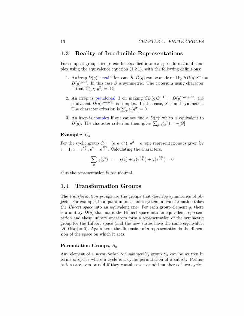
1.3 Reality of Irreducible Representations
For compact groups, irreps can be classified into real, pseudo-real and com-plex using the equivalence equation (1.2.1), with the following definitions:
1. An irrepD(g) is real if for some S, D(g) can be made real by SD(g)S−1 =D(g)real. In this case S is symmetric. The criterium using characteris that
∑g χ(g2) = [G],
2. An irrep is pseudoreal if on making SD(g)S−1 = D(g)complex, theequivalent D(g)complex is complex. In this case, S is anti-symmetric.The character criterion is
∑g χ(g2) = 0.
3. An irrep is complex if one cannot find a D(g)′ which is equivalent toD(g). The character criterium them gives
∑g χ(g2) = −[G]
Example: C3
For the cyclic group C3 = (e, a, a2), a3 = e, one representations is given by
e = 1, a = e2πi3 , a2 = e
4πi3 . Calculating the characters,∑
g
χ(g2) = χ(1) + χ(e4πi3 ) + χ(e
8πi3 ) = 0
thus the representation is pseudo-real.
1.4 Transformation Groups
The transformation groups are the groups that describe symmetries of ob-jects. For example, in a quantum mechanics system, a transformation takesthe Hilbert space into an equivalent one. For each group element g, thereis a unitary D(g) that maps the Hilbert space into an equivalent represen-tation and these unitary operators form a representation of the symmetricgroup for the Hilbert space (and the new states have the same eigenvalue,[H,D(g)] = 0). Again here, the dimension of a representation is the dimen-sion of the space on which it acts.
Permutation Groups, Sn
Any element of a permutation (or symmetric) group Sn can be written interms of cycles where a cycle is a cyclic permutation of a subset. Permu-tations are even or odd if they contain even or odd numbers of two-cycles.

1.4. TRANSFORMATION GROUPS 17
For example, S3 is the permutation on 3 objects, [e, a1 = (1, 2, 3), a2 =(3, 2, 1), a3 = (1, 2), a4 = (2, 3), a5 = (3, 1)], and (123)→ (12)(23) is even.
The order of Sn is N !. There is a simple N-dimensional representation ofSn called the defining representation, where permuted objects are the basisof a N vector space. Permutation groups appears on the relation of thespecial orthogonal groups as
Sn =SO(n+ 1)
SO(n).
Dihedral Group, D2n
The dihedral group is the group symmetry of a regular polygon, and thegroup has two basic transformations (called isometries), rotation , withdet=1,
gk =
(cos2πk
n −sin2πkn
sin2πkn cos2πk
n
),
and reflection, with det= -1,
σ =
(−1 00 1
).
The dihedral group is non-abelian8 if N > 2. A polyhedra in accordingto its dimension is categorized on table 1.1. The transformation groups actson vertices, half of vertices and cross-lines of symmetrical objects.
Dimension Object
d=0 Pointd=1 Lined=2 D2N
d=3 Polyhedrad=4 Polytopes
Table 1.1: Geometric objects related to their dimensions.
8For non-abelian groups, at least some of the representations must be in a matrix form,since only matrices can reproduce non-abelian multiplication law.

18 CHAPTER 1. FINITE GROUPS
Cyclic Groups, Zn
A cyclic group is a group that can be generated by a single element, g(called the generator of the group), such that when written multiplicatively,every element of the group is a power of g. For example, for the group Z3,described on section 1.3, the regular representation is
D(e) =
1 0 00 1 00 0 1
, D(a) =
0 0 11 0 00 1 0
, D(a2) =
0 1 00 0 11 0 0
.
One can see that for both, this above representation and the regularrepresentation of Zn, they can be made cyclic by the multiplication of thegenerator.
Another example is the parity operator on quantum mechanics [e, p],where p2 = 1. This group is Z2 and has two irreps, the trivial D(p) = 1and one in which D(e) = 1, D(p) = −1. On one-dimensional potentialsthat are symmetric on x = 0, their eigenvalues are either symmetric or anti-symmetric under x→ −x, corresponding to those two irreps respectively.
Alternating Groups, An
The alternating group is the group of even permutations of a finite set. Itis the commutator subgroup of Sn such that Sn/An = S2 = C2.

Chapter 2
Lie Groups
A Lie Group is a group which is also a manifold, thus there is a smallneighborhood around the identity which looks like a piece of RN , whereN is the dimension of the group. The coordinate unit vector Ta are theelements of the Lie algebra and an arbitrary element g close to the identitycan be always expanded into these coordinates as in (2.1.1). A Lie groupcan have several disconnected pieces and the Lie algebra specifies only theconnected pieces containing the identity.
2.1 Lie Algebras
In compact1 Lie Algebras, that are the interest here, the number of gen-erators T a is finite and the structure constant on the (2.1.2) are real andantisymmetric. Any infinitesimal group element g close to the identity canbe written as
g(a) = 1 + iaaTa +O(a2), (2.1.1)
where the multiplication of two group elements g(a), g(b),
[T a, T b] = ifabcT c, (2.1.2)
1In general, a set is compact if every infinite subset of it contains a sequence whichconverges to an element of the same set. A closed group, whose parameters vary over afinite range, is compact, every continuous function defined on a compact set is bounded.It defines a connected algebras, for example SO(4) is compact but SO(3,1) is not, or forinstance, a region of finite extension in an euclidian space is compact. The integral of acontinuous function over the compact group is well defined and every representation of acompact group is equivalent to a unitary representation.
19

20 CHAPTER 2. LIE GROUPS
is given by the non-abelian generators commutation relation. All the fourproprieties defined for finite groups verify for this continuous definition ofelements of groups. For instance, the closure is proved by making
eiλa1Taeiλ
b2Tb = eiλ
c3Tc = ei(λ
a1Ta+λb2Tb+
12
[λa1Taλb2Tb]).
U(N) Group of all N ×N unitary matrices.Lie algebra Set of N2 − 1 hermitians N ×N -matrices.
SO(N) Group of all N ×N orthogonal matrices.Lie algebra Set of 2N2 ±N complex antisymmetric N ×N matrices.
Table 2.1: Distinction among the elements of the group and the elements ofthe representation (the generators), for Lie groups.
Semi-Simple Lie Algebra
If one of the generators of the algebra commutes with all the others, itgenerates an independent continuous abelian group ψ → eiθψ, called U(1).If the algebra contains this elements it is semi-simple. This is the case ofalgebras without abelian invariant subalgebras, but constructed by puttingsimple algebras together. Invariant subalgebras (as defined before) are setsof generators that goes into themselves under commutation. A mathematicalway of expressing it is by means of ideals. A normal/invariant subgroup isgenerated by an invariant subalgebra, or ideal, I, where for any element ofthe algebra, L, [I, L] ⊂ I. A semi-simple group has no abelian ideals.
Non semi-simple Algebra Contains ideals I where [I, L] ⊂ ISemi-simple Algebra All ideals I are non-abelian [I, L] 6= 0 ⊂ I
Simple Algebra No Ideals, only trivial invariant subalgebra.
Table 2.2: Definition algebras in terms of ideals.
A generic element of U(1) is eiθ and any irrep is a 1× 1 complex matrix,which is a complex number. The representation is determined by a chargeq, with the group element g = eiθ represented by eiqθ. In a lagrangian withU(1) symmetry, each term on the lagrangian must have the charges add upto zero.

2.1. LIE ALGEBRAS 21
Every complex semi-simple Lie algebra has precisely one compact realform. In semi-simple Lie algebras every representation of finite degrees isfully reducible. The necessary and sufficient condition for a algebra to besemi-simple is that the Killing metric is non-singular, (2.4.4), gαβ 6= 0, i.e.it has an inverse gαβgβν = δαν . If gαβ is negative definite, the algebra iscompact, thus it can be rescaled in a suitable basis gαβ = −δαβ.
Non Semi-Simple Lie Algebra
A non semi-simple Lie algebra A is a direct sum of a solvable Lie algebra(P) and a semi-simple Lie algebra (S). The definition of solvable Lie algebrais giving by the relation of commutation of the generators,
[A,A] = A1
[A1, A1] = AK ,
....
where if at some point one finds [An, An] = An+1 = 0, the algebra is solvable.
Example: The Poincare Group
Recalling the generators of the Poincare group SO(1,3), one has the semi-simple (simple + abelian) and the solvable:
[M,M ] = M, Simple,
[P, P ] = 0, Abelian,
[M,P ] = P, Solvable sector.
Simple Lie Algebra
A simple Lie algebra contains no deals (it cannot be divided into two mu-tually commuting sets). It has no nontrivial invariant subalgebras.
The generators are split into a set H, which commutes to each other,and the rest, E, which are the generalized raising and lowering operators.The classification of the algebra is specified by the number of simple roots,whose lengths and scalar products are restricted and can be summarized bythe Cartan matrix and the Dynkin diagrams.

22 CHAPTER 2. LIE GROUPS
For simple compact Lie groups, the Lie algebra gives an unique simplyconnected group and any other connected group with same algebra must bea quotient of this group over a discrete identification map. For instance,the Lie algebra of rotations SU(2) and the group SO(3) have the same Liealgebra but they differ by 2π, which is represented in SU(2) by diag (-1,1)2.
The condition that a Lie Algebra is compact and simple restricts it to 4infinity families (An, Bn, Cn, Dn) and 5 exceptions (G5, F4, E6, E7, E8). Thefamilies are based on the following transformations:
Unitary Transformations of N-dimensional vectors For η, ξ, N-vectors,with linear transformations ηa → Uabηb and ξa → Uabξb, this subgrouppreserves the unitarity of these transformations, i.e. preserves η∗aξ
a.The pure phase transformation ξae
iαξa is removed to form SU(N),consisting of all N ×N hermitian matrices satisfying det(U)=1. TheN2 − 1 generators of the group are the N ×N matrices T a under thecondition tr[T a] = 0.
Orthogonal Transformations of 2N-dimensional vectors The subgroupof orthogonal 2N × 2N transformations that preserves the symmetricinner product: ηaEabξb with Eab = δab, which is the rotation group in2N dimensions, SO(n) (we will use n = 2N and n = 2N + 1). Thereis an independent rotation to each plane in n dimensions, thus thenumber of generators are n(n−1)
2 , or 2N2 ±N .
Symplectic Transformations of N-dimensional vectors The subgroupof unitary N × N transformations where for N even, it preserves theantisymmetric inner product ηaEabξb, where
Eab =
(0 1−1 0
).
The elements of the matrix are N2 ×
N2 blocks, defining the symplectic
group Sp(n), with n(n+1)2 or 2N2 +N generators.
2.2 Representations
Matrices associated with elements of a group are a representation of thisgroup. Every group has a representation that is singlet or trivial, in which
2SO(3)/SU(2) ' Z2.
2.2. REPRESENTATIONS 23
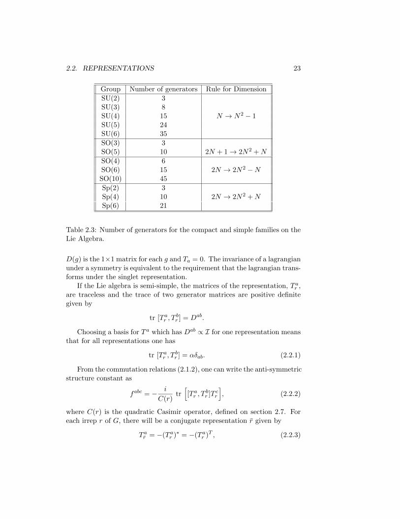
Group Number of generators Rule for Dimension
SU(2) 3SU(3) 8SU(4) 15 N → N2 − 1SU(5) 24SU(6) 35
SO(3) 3SO(5) 10 2N + 1→ 2N2 +N
SO(4) 6SO(6) 15 2N → 2N2 −NSO(10) 45
Sp(2) 3Sp(4) 10 2N → 2N2 +NSp(6) 21
Table 2.3: Number of generators for the compact and simple families on theLie Algebra.
D(g) is the 1×1 matrix for each g and Ta = 0. The invariance of a lagrangianunder a symmetry is equivalent to the requirement that the lagrangian trans-forms under the singlet representation.
If the Lie algebra is semi-simple, the matrices of the representation, T ar ,are traceless and the trace of two generator matrices are positive definitegiven by
tr [T ar , Tbr ] = Dab.
Choosing a basis for T a which has Dab ∝ I for one representation meansthat for all representations one has
tr [T ar , Tbr ] = αδab. (2.2.1)
From the commutation relations (2.1.2), one can write the anti-symmetricstructure constant as
fabc = − i
C(r)tr[[T ar , T
br ]T cr
], (2.2.2)
where C(r) is the quadratic Casimir operator, defined on section 2.7. Foreach irrep r of G, there will be a conjugate representation r given by
T ar = −(T ar )∗ = −(T ar )T , (2.2.3)

24 CHAPTER 2. LIE GROUPS
if r ∼ r then T ar = UT ar U† and the representation is real or pseudo-real, if
there is no such equivalence, the representation is complex.The two most important irreducible representations are the fundamental
and the adjoint representations:
Fundamental In SU(N) the basic irrep is the N-dimensional complex vec-tor, and for N > 2, this irrep is complex. In SO(N) it is real and inSp(N) it is pseudo-real.
Adjoint It is the representation of the generators, [r] = [G], and the repre-sentation’s matrices are given by the structure constants (Ta)bc = −fabcwhere ([T bG, T
cG])ae = if bcd(T dG)ae. Since the structure constants are
real and anti-symmetric, this irrep is always real.
2.3 The Defining Representation
A subset of commuting hermitian generators which is as large as possible iscalled the Cartan subalgebra, and it is always unique. The basis are calleddefining (fundamental) representation and are given by the colum -vectors(1, 0, 0, .., 0)N , etc. In an irrep, D, there will be a number of hermitiangenerators, Hi for i = 1 to k, where k is the rank of the algebra, that arethe Cartan Generators:
Hi = H†i ,
[Hi, Hj ] = 0. (2.3.1)
The Cartan generators commute with every other generator and forma linear space. One can choose a basis satisfying the normalization (from(2.2.1)),
tr (HiHj) = λδij ,
for i, j = 1 to N − 1. For the group SU(N) λ = 12 . The states of the
representation D can be written as
Hi|µ, x,D〉 = µi|µ, x,D〉, (2.3.2)
where µi are the weights. The number of weights the fundamental represen-tion is equal to the number of vectors on the fundamental representation,but their dimension is the dimension of the rank. For example on SU(3),

2.4. THE ADJOINT REPRESENTATION 25
one has 3 orthogonal vectors (v1 = (1, 0, 0), for instance) on the fundamentalrepresentation and 3 weights (µ1 = (1
2 ,1
2√
3), for instance).
The contraction of a fundamental and an anti-fundamental field form assinglet is N ⊗N = (N2 − 1)⊕ 1.
2.4 The Adjoint Representation
The adjoint representation of the algebra is given by the structure constants,which are always real,
[Xa, Xb] = ifbcdXc. (2.4.1)
[Xa, [Xb, Xc]] = ifbcd[Xa, Xd] = −fbcdfadeXe.
If there are N generators, then we find a N ×N matrix representationin the adjoint representation. From the Jacobi identity,
[Xa[Xb, Xc]] + [Xb[Xc, Xa]] + [Xc[Xa, Xb]] = 0, (2.4.2)
one has similar relation for the structure constants,
fbcdfade + fabdfcde + fcadfbde = 0.
Defining a set of matrices Ta as
[Ta]bc ≡ −ifabc,
it is possible to recover (2.1.2):
[Ta, Tb] = ifbcdTc.
The states of the adjoint representation correspond to the generators|Xa〉. A convenient scalar product is:
〈Xa|Xb〉 = λ−1 tr (X†aXb).
The action of a generator in a state is:
Xa|Xb〉 = |Xc〉〈Xc|Xa|Xb〉= |Xc〉[Ta]cb= ifabc|Xc〉= |ifabcXc〉= |[Xa, Xb]〉.
26 CHAPTER 2. LIE GROUPS
The Killing Form
The Killing form is the scalar product of the algebra, defined in terms of theadjoint representation. Applying it to the generators themselves, it gives themetric gαβ of the Cartan matrices. The anti-symmetrical structure constants
fαβγ = fγ′
αβgγ′γ have the Killing metric given by
gγ′γ = fpγ′fpγ (2.4.3)
= tr T adjγ′ Tadjγ , (2.4.4)
recalling (T adjα )γβ = fγβα, the trace is independent of the choice of basis.
Application on Fields
A good way of seeing the direct application of this theory on fields is, forexample, the covariant derivative acting on a field in the adjoint represen-tation:
(Dµφ)a = ∂µφa − igAbµ(taG)bcφc,
= ∂µφa + gfabcAbµφ
c,
and the vector field transformation is
Aaµ → Aaµ +1
g(Dµ)a.
2.5 The Roots
The roots are weights (states) of the adjoint representation, in the same waythey were defined to the Cartan generators, (2.3.2), where from (2.3.1), wesee that
Hi|Hj〉 = |[Hi, Hj ]〉 = 0.
Therefore, all states in the adjoint representation with zero weight vectorsare Cartan generators (and they are orthonormal). The other states havenon-zero weight vectors α,
Hi|Eα〉 = αiEα. (2.5.1)

2.5. THE ROOTS 27
The non-zero roots uniquely specify the corresponding states, Eα, and theyare the non-hermitian raising/lowering operators:
[Hi, Eα] = αiEα, (2.5.2)
[Hi, E†α] = −αiE†α, (2.5.3)
E†α = E−α, (2.5.4)
[Eα, E−α] = −αH, (2.5.5)
where we can set the normalization (in the same fashion as (2.4.3)) as
〈Eα|Eβ〉 = λ−1 Tr (E†αEβ) = δαβ.
From (2.5.5), for any weight µ of a representation D, setting H = E3,one has
E3|µ, x,D〉 =αµ
|α|2|µ, x,D〉, (2.5.6)
which are always integers or half-integers and it is the origin of the MasterFormula. From this equation, we can see that all roots are non-degenerated,
2α.µ
α2= −p+ q, (2.5.7)
where p is the number of times the operator Eα may raise the state and q,the number of times the operator E−α may lower it.
Roots α
The roots can be directly calculated from the the weights of the Cartangenerators by ±αij = µi ± µj .
Positive Roots
When labeling roots in either negative or the positive, one can set the wholeraising/lowering algebra. It is convention, for instance one can set for SU(N)the positive root to be the first non-vanishing entry when it is positive.
One can define an ordering of roots in the way that if µ > ν than µ− νis positive, and from this finde the highest weight of the irrep. In the adjointrepresentation, positive roots correspond to raising operators and negativeto lowering operators.

28 CHAPTER 2. LIE GROUPS
Simple Roots ~α
Some of the roots can be built out of others, and simple roots are the positiveroots that cannot be written as a sum of other positive roots. A positiveroot is called a simple root if it raises weights by a minimal amount. Everypositive root can be written as a positive sum of simple roots. If a weight isannihilated by the generator of all the simple roots, it is the highest weight,ν, of an irreducible representation. From the geometry of the simple roots,it is possible to construct the whole algebra,
• If ~α and ~β are simple roots, then ~α− ~β is not a root (the difference oftwo roots is not a root).
• The angles between roots are π2 ≤ θ < π.
• The simple roots are linear independent and complete.
Fundamental Weights ~q
Every algebra has k (rank of the algebra) fundamental weights that are abasis orthogonal to the simple roots α, and they can be constructed fromthe master formula, (2.5.7), with a metric gij , (2.4.4), to be defined,
2qIi g
ijαJj
αJj gijαJj
= δIJ , (2.5.8)
If we use of the Killing metric defined on (??), for SU(N), the relationbecomes
2qjαk
|αk|2= δjk. (2.5.9)
All irreps can be written in terms of the fundamental weight and thehighest weight as
νHW =k∑i=1
aiqi = a1q
1 + a2q2 + ...+ aNq
k, (2.5.10)
where ai are the Dynkin coefficients, ai = qi − pi.

2.5. THE ROOTS 29
The Master Formula
We have already seen the role of the master formula on equations (2.5.6)and (2.5.7), now let us derive it properly. Supposing that the highest stateis j, there is some non-negative integer p such that (E+)p|µ, x,D〉 6= 0, withweight µ + pα, and which (E+)p+1|µ, x,D〉 = 0. The former is the higheststate of the algebra.The value of E3 is then
α(µ+ pα)
α2=αµ
α2+ p = j. (2.5.11)
On another hand, there is a non-negative integer q such that (E−)q|µ, x,D〉 6=0, with weight µ − qα, being the lowest state, with (E−)q+1|µ, x,D〉 = 0.The value of E3 is then
α.(µ− qα)
α2=α.µ
α2− q = −j. (2.5.12)
Adding (9.2.2) and (9.3.4) one has the formulation of the master formula,as in (2.5.7),
α.µ
α2= −1
2(p− q).
Subtracting (9.2.2) from (9.3.4) one have the important relation
p+ q = 2j. (2.5.13)
Construction of Irreps of SU(3) from the Highest Weight ν 3
It is possible to construct all representations of an irrep of any Lie algebrarepresented by its highest weight. One needs only to know a basis for thefundamental weights and their orthogonal simple roots of the group and tomake use of the theory of lowering and raising operators. Let us show anexample of a irrep of SU(3) with highest weight ν = q1 + 2q2, where q1, q2
are the fundamental weight of SU(3).Recalling from table 3.4, the simple roots and the fundamental weights
of SU(3), the highest weight of the irrep we are going to construct is
ν = q1 + 2q2 = (3
2,− 1
2√
3).
3Exercise proposed by Prof. Nieuwenhuizen[?].

30 CHAPTER 2. LIE GROUPS
From the master formula, (2.5.7), for each of the two simple roots (wherewe consider them normalized |α1|2 = 1 = |α2|2),
2αiν =1
2q,
where p = 0 since this is the highest weight. Calculating for the both simpleroots,
α1ν = q1 = 1,
α2ν = q2 = 2.
The first vectors are then
|ν〉, |ν − α1〉, |ν − α2〉, |ν − 2α2〉.
We now lower, in the same fashion, |ν − α1〉, with E−α2 , and |ν − α2〉,|ν − 2α2〉 with E−α1 ,
2α2(ν − α1) = q12 = 3,
giving 3 more vectors, |ν − α1 − α2〉, |ν − α1 − 2α2〉, |ν − α1 − 3α2〉.
2α1(ν − α2) = q21 = 2,
giving 2 more vectors, but only one new, |ν − α1 − 2α2〉.
2α1(ν − 2α2) = q211 = 2,
giving two more new vectors, |ν − 2α1 − 2α2〉, ν − 3α1 − 2α2〉.The weights will sum up 15, which is exact the dimension of this irrep
on SU(3).
2.6 The Cartan Matrix and Dynkin Diagrams
The Cartan matrices represent directly the proprieties of the algebra of eachLie family and are constructed from the master formula, (2.5.7), multiplyingall simple roots αi among themselves,
Aij = 2αiαj
|αi|2. (2.6.1)
The off-diagonal elements can only be 0, -1, -2 and -3. If all roots havethe same length, A is symmetric, and if Aij 6= 0 then Aji 6= 0. The rowsof the Cartan matrix are the Dynkin coefficients (labels) of the simple root,and are directly used on the constructed of the algebra.

2.6. THE CARTAN MATRIX AND DYNKIN DIAGRAMS 31
The Dynkin diagram is a diagram of the algebra of the groups in termsof angles and size of the roots. Multiplying the master formula by itself,and using the Schwartz inequality4, we can define the angles between theproduct of two simple roots as
cos θ12 =α1α2
|α21||α1
1|=
1
4
√n1n2,
with the limited possibilities on n1n2 < 4. The conditions for the two rootsare then
1. n1 = n2 = 0, θ = π2 , the two roots are orthogonal and there is no
restriction of length. Aij = 0, the roots are not connected.
2. n1 = n2 = 1, θ = π3 , and |α1| = |α2|. Aij = −1, the roots have the
same length.
3. n1 = 2, n2 = 1, θ = π4 , |α2| =
√2|α1|. Aij = −2, the roots have value
2 and 1.
4. n1 = 3, n2 = 1, θ = π6 , |α2| =
√3|α1|. Aij = −3, the highest root has
value 3.
Summarizing, the rules to construct the Dynkin diagram for some Liealgebra are the following:
1. For every simple root, one writes a circle.
2. Connect the circles by the number of lines given by Aij of (2.6.1). Twocircle are joined with one line if θ = π
3 , two lines if θ = π4 , and three
lines if θ = π6 .
3. For a semi-simple algebra the diagram will have disjoint pieces, forexample, SO(4) ' SU(2) × SU(2), which is not simple, is giving bytwo disconnected circles.
4. When the length are unequal, one can either write an arrow pointingto the root of smaller length, or write all small roots as a black dot.
From the Dynkin diagrams it is possible to check if two groups are locallyisomorphic and the sequence for compact and simple Lie groups is
4The Cauchy-Schwarz inequality states that for all vectors x and y of an inner productspace, |〈x, y〉|2 ≤ 〈x, x〉 · 〈y, y〉.

32 CHAPTER 2. LIE GROUPS
Groups Dynkin Diagram
SO(3) ' SU(2)'USp(2) SO(4) 'SU(2)×SU(2)
SO(5)'USp(4) = SO(6)' SU(4) − −
Table 2.4: Local isomorphism among the Cartan families.
A regular subalgebra is obtained by deleting points from the Dynkindiagram. For example, SU(2)⊕SU(4) ⊂ SU(6) and its six dimensions givea regular representation of the regular subalgebra of SU(2) (1,2) and SU(4)(4,1). The non-regular subalgebra SU(3)⊕ SU(2) gives an irrep (3,2).
There is a symmetric invariant bilinear form for the adjoint representa-tion
SU(N) ⊂ SO(N2 − 1). (2.6.2)
2.7 Casimir Operators
If the Lie algebra is semi-simple, then the metric (2.4.4) has determinantnon-zero (detgαβ 6= 0). In this case, an irrep R has the Casimir operatordefined as
C2(R) = gαβTRα TRβ , (2.7.1)
where TR are the chosen generators and the metric has the compactnesscondition
gαβ = f qαβfppq ≤ 0,
and the commutation relation of the Casimir operator to all other generatorsis zero,
[C2(R), TRa ] = 0.
Proof.
[gαβTαTβ, Tγ ] = gαβTα[Tβ, Tγ ] + gαβ[Tα, Tγ ]Tβ
= fαδγ (TRα Tkδ + T kδ T
Rα )
= 0.

2.7. CASIMIR OPERATORS 33
Using the Schur’s lemma on (2.7.1), it is clear that since C2(R) commutesto all other generators, it must be proportional to the identity,
C2(R) = C2(R)I,
where C2(R) is the Quadratic Casimir Invariant of each irrep, which is aninvariant of the algebra. It has a meaning only for representations, not asan element of the Lie algebra, since the product (2.7.1) are not defined forthe algebra itself, but only for the representations.
For compact groups, the Killing form is just the Kronecker delta, forexample on SU(2), the Casimir invariant is then simply the sum of thesquare of the generators Lx, Ly, Lz of the algebra, i.e., the Casimir invariantis given by L2 = L2
x + L2y + L2
z. The Casimir eigenvalue in a irrep is justL2 = l(l + 1). For example for the adjoint irrep,
facdf bcd = C2(G)δab,
a symmetric invariant two-indice tensor δαβ = δβα is unique up rescaling
(T adjγ )βα, therefore it is possible to write tr TRα TRβ = δRαβ = δαβT (R).
To compute explicitly T(R), one starts with any Lie algebra tr TαTβ =T (R)gαβ, and the Casimir operators can be found from knowing the dimen-sion of the irrep R and the group G,
C2(R)× dim R = dim G× T (R), or, (2.7.2)∑a
Ta(R)2 = C2(R)× 1d(R)×d(R). (2.7.3)
For the fundamental representation of SU(N), C2(R) = N2−12N . For the
adjoint representation C2(G) = C(G) = N . For the spinorial representationof SO(2N), C2(G) = 2N−4. The number of generators required to give acomplete set of these invariants is equal to the rank.
Harish-Chandra Homomorphism
The center of the algebra of the semi-simple Lie algebra is a polynomial alge-bra. The degrees of the generated algebra are the degree of the fundamentalinvariants. The number of invariants on each family is shown on table 2.5.
Example: The fundamental irrep 3 of SU(3)
For the irrep 3 of SU(3), one has the generators given by
Ta(3) =λa2,

34 CHAPTER 2. LIE GROUPS
An I2, I3, ..., In+1
Bn I2, I4, ..., I2n
Cn I2, I4, ..., I2n
Dn I2, I4, ..., I2n−2
Table 2.5: Order of the independent invariants for the four Lie families.
and the dimension of the group is N2 − 1 = 8 resulting
tr∑a
(λa2
)2 =∑a
1
2δaa =
1
2× 8→ 3C2(3),
the quadratic Casimir invariant is then
C2(3) =4
3.
Example: The adjoint irrep 8 of SU(3)
Now one has
Ta(8) = ifabc,
where
−∑a
fabcfdbc = C2(8)δad.
The quadratic Casimir invariant is given by
8C2(8) = f2abc = 6(1 +
6
4+
23
24) = 24,
C2(8) = 3.
2.8 *Weyl Group
For every root m there is a state with −m: large algebras have reflectionsymmetries and the group generated by those reflections are the Weyl group.This group maps weights to weights.

2.9. *COMPACT AND NON-COMPACT GENERATORS 35
2.9 *Compact and Non-Compact Generators
The number of compact generators less the number of non-compact is therank of the Lie Algebra, which is the maximum number of commuting gener-ators. On table 2.6 the Cartan series are separated in terms of their compactand non-compact generators, which is given by the following algebra.
[C,C] = C,
[C,NC] = NC,
[NC,NC] = C.
An, SU(N+1) N compact Ti where [Ti, Tj ] = εijkTk.
An, SL(N,C) SL(N,R), non-compact: all generators of SU(N) times i.
SU(p,q), non-compact,∑p
i=1(xi)∗xi =∑N
j=p+1(xj)∗xj .
Bn, SO(2N+1,C) SO(2N+1,R), real, compact.
SO(p,q,R), non-compact,∑p
i=1(xi)2 =
∑Nj=p+1(xj)2.
Dn, SO(2N,C) SO(2N,R), real, compact.SO(p,q), p+1=2N, non-compact.
Examples: Anti-deSitter superalgebra, SO(4,1), SO(2,N)∗,deSitter superalgebra SO(3,2), SO(N).
Table 2.6: The Lie groups in terms of the compact and non-compact gener-ators.
Example of non-compact groups are SU(p,q) (which preserves the formx†1p,qy) and SL(N,R), which is the group of N×N real matrices with unitarydeterminant. One can go from compact groups to non-compact versions byjudiciously multiplying some of the generators by i (or equivalently, letting

36 CHAPTER 2. LIE GROUPS
some generators become pure imaginary). The general procedure for associ-ating a non-compact algebra with a compact one is first to find the maximalsubalgebra and then multiply the remaining non-compact generators by i.
2.10 *Exceptional Lie Groups
The process of constructing the algebra for the five Cartan exceptionalgroups G2, F4, E6, E7, E8, consists basically on the following method:
1. Choose an easy subgroup H of G and a simple representation of thisH. This should be the Maximal Regular subgroup, i.e. an algebrawhich has the same rank thus we can write the Cartan generatorsof the group as a linear combination of the Cartan generators of thesubgroup, and there is no large subalgebra containing it except thegroup itself.
2. Decompose the representation R into irreps Ri of H, and how it actsin Ri. An irrep of an algebra becomes a representation of the subal-gebra when its is embedded by a homomorphism that preserves thecommutation relations.
3. Construct the Lie algebra of G starting with the Lie algebra of H andRi of H.
For example, mainly from (2.6.2) one can find the following: E6 has amaximal regular subalgebra in SU(6) ⊗ SU(2), E7 has a maximal subal-gebra in SU(8), and and E8 has a maximal regular subalgebra in SO(16).The lowest dimensional irrep of E8 is the adjoint irrep with 24-dimensionalgenerators, which can be used on the above process.
As a remark, before these exceptional families, the first groups are ac-tually locally isomorphic to the four Lie families, E5 ' SO(10), E4 'SU(3)× SU(2), and E3 ' SU(2)× SU(2).

Chapter 3
SU(N), the An series
SU(N) is the group of N × N unitary matrices, U †U = 1 with det U = 1.The rank of SU(N) is N − 1 and the number of generators is N2 − 1. Thetraceless constraint tr(ααTα) = 0 is what gives the determinant a unitaryvalue.
Proof. Any element of the group can be represented as
U(α)→ eiαT
and can be diagonalized by
UαTU−1 = D,
Now, taking the determinant,
det U(α) = det (eiD)
= ei tr D
= ei tr αT .
= 1.
3.1 The Defining Representation
SU(N) has N objects φi, i = 1, ..., N that transform under φi → φ′i = U ijφj .
The complex conjugate transforms as φ∗i → φ′∗i = (U ij)∗φ∗j = (U †)jiφ
∗j .
37

38 CHAPTER 3. SU(N), THE AN SERIES
There are higher representations, for example, the tensor φijk , transformas they were equal to multiplication of the vectors, φiφjφk,
φijk → U ilUjm(U †)nkφ
lmn .
The trace is always a singlet and it can be separated by setting theupper index equals to the lower index, φijj → U il φ
lmm , and subtracting it
from the original tensor. In this way, the tensor φijk can be decomposed intosets containing 1
2N2(N + 1)−N symmetric traceless and 1
2N2(N − 1)−N
anti-symmetric traceless components. More examples can be seen on table3.1.
Element Dimension Description Dimension on SU(5)
φi N Defining Irrep 5
φij N2 N ⊗N Defining 25φij N2 − 1 N ⊗ N − U(1), Adjoint irrep 24
φij N(N+1)2 Symmetric 15
φij N(N−1)2 Anti-symmetric 10
φijk N3 N ⊗N ⊗N , Defining 125
φijk12N
2(N + 1)−N Symmetric traceless 70
φijk12N
2(N − 1)−N Anti-symmetric traceless 45φikk 2N Trace 10
Table 3.1: The decomposition of SU(N) into its irreps.
3.2 The Cartan Generators H
The Cartan-Weyl basis for the group SU(N) are the maximally commutativebasis of N − 1 generators, N − 1, given can given by the following basis ofmatrices, which are a generalization of the Gell-Mann matrices:
HI =1
2
1 0 0 0 00 −1 0 0 00 0 0 0 00 0 0 0 00 0 0 0 ...
N×N

3.3. THE WEIGHTS µ 39
HII =1
2√
3
1 0 0 0 00 1 0 0 00 0 −2 0 00 0 0 0 00 0 0 0 ...
N×N
HIII =1√24
1 0 0 0 00 1 0 0 00 0 1 0 00 0 0 −3 00 0 0 0 ...
N×N
...
HN−1 =1√
2N(N − 1)
1 0 0 0 00 1 0 0 00 0 1 0 00 0 0 1 00 0 0 ... −(N − 1)
N×N
3.3 The Weights µ
The weights of the defining representation, from the Cartan generators, areN -vectors with N − 1-entries each, given by
µI = (1
2,
1
2√
3,
1√24, ...,
1√2N(N − 1)
),
µII = (−1
2,
1
2√
3,
1√24, ...,
1√2N(N − 1)
),
µIII = (0,− 1√3,
1√24, ...,
1√2N(N − 1)
),
...
µN = (0, 0, 0, ...,−(N − 1)√2N(N − 1)
),
3.4 The Roots α
The roots are the weights of the generators that are not Cartan. There areN(N−1) roots on SU(N) and together with N weights, they give N2, whichis one plus the number of total generators (given by N2 − 1). The roots onSU(N) are generated by the commutation between these generators,
[H,Eα] = αiEα,

40 CHAPTER 3. SU(N), THE AN SERIES
[H,Eαij ] = (µi − µj)Eαij ,
± αij = µi − µjj. (3.4.1)
The Positive Roots
The positive roots are given by the first non-vanishing positive entry. Thereare N(N−1)
2 positive roots on SU(N).
The Simple Roots ~α
Simple roots are positive roots that cannot be constructed by others. Thenumber of simple roots is the equal to the rank k of the algebra, wherek = N − 1 in the case of SU(N). In resume, to find the simple roots, onecalculates all possible roots by
~αij = µi − µj , (3.4.2)
= µi − µi+1 → α12, α23, .., αN−1,N , (3.4.3)
finds the positives roots, and then check which are not the sum of others(totalizing N − 1 simple roots).
When associating roots and fundamental weights to the Dynkin dia-grams, we see that the fundamental highest weights are the first weight ofthe defining representation and its complex conjugate (last weight). Thesymmetric product of two vectors (2-fold) gives two HW (2,0,0...), the sym-metric product of three vectors (3-fold) gives (3,0,0,0..), etc. The 3-foldanti-symmetric product contains a rep that is the sum of 3 HW, (0,0,1,0...),the two-fold anti-symmetric (0,1,0,...). To illustrate them, the highest weightfor some representations for SU(6) are shown on table 3.2.
3.5 The Fundamental Weights ~q
The k = N − 1 fundamental weights of a Lie algebra are given by theirorthogonality to the simple roots, relation that can be checked with themaster formula (2.5.7),
2αI~qJ
|α|2= δIJ . (3.5.1)
For SU(N), one can also write the fundamental weights in a basis doing
qi = µi − µi+1

3.6. THE KILLING METRIC 41
Representation HW on the Dynkin Diagram
Fundamental − − − 1 - 0 - 0 - 0 - 0
Anti-fundamental − − − 0 - 0 - 0 - 0 -1
2-fold Symmetric − − − 2 - 0 - 0 - 0 -0
2-fold Anti-symmetric − − − 0 - 1 - 0 - 0 - 0
Adjoint − − − 1 - 1 - 0 - 0 - 0
Table 3.2: The highest weight of all irreps of SU(6).
q1 = µ1 − µ2, q2 = µ2 − µ3, q3 = µ3 − µ4....
resulting on
qI = (1, 0, 0, 0...0),
qII = (−1
2,
√3
6, 0, 0...0),
qIII = (0,−√
3
3,
√24
6, 0...0),
...
3.6 The Killing Metric
The Killing metric for SU(N) is
gij = tr HiHj ,
=1
2δij .
3.7 The Cartan Matrix
The Cartan matrix, calculated from the equation 2.6.1, from last chapter,
Aij = 2αiαj
|αi|2.

42 CHAPTER 3. SU(N), THE AN SERIES
has the form following form on SU(N):
A =
2 −1 0 ... 0 0 0−1 2 −1 ... 0 0 00 −1 2 ... −1 0 00 0 −1 ... 2 −1 00 0 0 ... −1 2 −10 0 0 ... 0 −1 2
.
3.8 SU(2)
In the special unitary subgroup of two dimensions, any element can be writ-ten as
g =
(a −bb a
),
where |a2| + |b2| = 1. The elements of the group are represented by eλaTa ,with Ta antihermitian and given by the Pauli matrices,
Ta =1
2σa.
Since in SU(2) the structure constant εij carries only two indices, itsuffices to consider only tensors with upper indices, symmetrized. As aconsequence, we are going to see that SU(2) only has real and pseudo realrepresentations.
The Defining Representation
The Cartan generator is given by the maximal hermitian commutating basis,composed only of H, since the rank is 1. Recalling the traditional algebrafrom Quantum Mechanics, for the vectors that spam the fundamental defin-ing representation, (1,0) and (0,1), and making H = J3, we have
[J3, J±] = ±J±,
H = J3 =1
2σ3.
The Weights µ
The eigenvalue of H are the weights
• H(
10
)= 1
2
(10
), µI1 = 1
2 .

3.9. SU(3) 43
• H(
01
)= −1
2
(01
), µII1 = −1
2 .
The Raising/ Lowering Operators
The Raising/ Lowering Operators are given by
E+ = J1 + iJ2 =1
2(σ1 + iσ2),
E− = J1 − iJ2 =1
2(σ1 − iσ2).
Extending these results, we see that for each non-zero pair of root vector±α, there is a SU(2) subalgebra with generators
E± ≡ |α|−1E±α,
E3 ≡ |α|−2αH.
The generators, the weights and the simple root of the defining (funda-mental) representation are shown on table 3.3.
Cartan generator H 12σ3
Raising operator E+ 12(σ1 + iσ2)
Lowering operator E− 12(σ1 − iσ2)
Weight I µI 12
Weight II µII −12
Simple Root I ~α12 1Fundamental Weight I ~q 1
Table 3.3: The generators, weights, simple root and fundamental weight ofthe defining representation of SU(2).
3.9 SU(3)
The elements of SU(3) are given by ebaTa , with ba real and Ta traceless andantihermitian that can be constructed from the original Gell-Mann matrices,λa,
Ta =1
2λa.

44 CHAPTER 3. SU(N), THE AN SERIES
From these matrices one has three compact generators, which are thosefrom SU(2) plus five extra non-compact generators. The number of compactgenerators less the number of non-compact is the rank of the Lie Algebra,k, which is the maximum number of commuting generators. In this casek = 3− 1 = 2, giving the two Cartan generators
H1 =1
2
1 0 00 −1 00 0 0
=1
2λ3
H2 =1
2√
3
1 0 00 1 00 0 −2
=1
2√
3λ8
The other N2 − 1− k = 6 generators of SU(3), are
λ1,2,3 =
σi 00
0 0 0
, λ4 =
0 0 10 0 01 0 0
λ5 =
0 0 −i0 0 0−i 0 0
λ6 =
0 0 00 0 10 1 0
, λ7 =
0 0 00 0 −i0 −i 0
, λ8 =1
2√
3
1 0 00 1 00 0 −2
The Defining Representation
The vectors
100
,
010
and
001
are the basis of the defining representa-
tion.
The Weights µ
The eigenvalues of the Cartan generators on the defining representation givethe threes weights of this algebra,
µI = (1
2,
1
2√
3),
µII = (−1
2,
1
2√
3),
µIII = (0,− 1√3
).

3.9. SU(3) 45
The Raising/ Lowering Operators
The raising/ lowering operators of SU(3) are
EIα = i(λ1 + iλ2) =
0 1 00 0 00 0 0
,
EIIα = i(λ4 + iλ5) =
0 0 10 0 00 0 0
,
EIIIα = i(λ6 + iλ7) =
0 0 00 0 10 0 0
,
EI−α = i(λ1 − iλ2) =
0 0 01 0 00 0 0
,
EII−α = i(λ4 − iλ5) =
0 0 00 0 01 0 0
,
EIII−α = i(λ6 − iλ7) =
0 0 00 0 00 1 0
The Roots α
The roots are the weight (states) of the adjoint representation. The firstgenerator can be written as
[H1, EαI ] = EIα,
[H2, EαI ] = 0,
concluding that the roots is αI+ = (1, 0), and the root of (EIα)† = EI−α is justthe same vector with opposite sign, αI− = (−1, 0) . For the second generatorand its complex conjugate,
[H1, EαII ] =1
2EIIα ,

46 CHAPTER 3. SU(N), THE AN SERIES
[H2, EαII ] =
√3
2EIIα ,
thus the root are ±αII = ±(12 ,√
32 ). For the third generator, the roots are
±αIII = ±(−12 .√
32 ).
The Simple Roots ~α
The simple roots of SU(3) are those that cannot be constructed by summingany two positive roots,
~αI = (1
2,
√3
2)
~αII = (1
2,−√
3
2).
The Fundamental Weights ~q
The two fundamental weights on SU(3) represent the 3 and 3 irreps. Byapplying (3.5.1) one gets (1
2 ,1
2√
3) and (1
2 ,−1
2√
3).
The Cartan Matrix
From (2.6.1), the product of the two simple roots are given by
cos θ11 = 2~α1~α1 = −2,
cos θ12 = 2~α1~α2 = −1,
cos θ22 = 2~α2~α2 = −2.
ASU(3) =
(2 −1−1 2
).
The group SU(3) has an important role on phenomenology of elementaryparticles. For instances one can represents mesons (quark and anti-quark)as 3 ⊗ 3 = 8 ⊕ 1, ψa ⊗ ψb = (ψaψ
b − 13δbaψcψ
c) + 13δbaψcψ
c, and baryons (3quarks) as 3⊗ 3⊗ 3 = 10⊕ 8⊕ 8⊕ 1, ψa ⊗ ψb = 1
2(ψ(aψb) + ψ[aψb]).
Example2: Working out in another Representation of SU(3)
Let us suppose another (natural) way of choosing Hj and E±α, given by
2Exercise proposed by Prof. Nieuwenhuizen.

3.9. SU(3) 47
Cartan generators H3, H812λ3, 1
2λ8
Raising operator E+αi , i = 1, 2, 4, 5, 6, 7 12(λi + λj)
Lowering operator E−αi , i = 1, 2, 4, 5, 6, 7 12(λi − λj)
Weight I µI (12 ,
12√
3)
Weight II µII (−12 ,
12√
3)
Weight III µIII (0, −1√3)
Simple Root I ~αI (12 ,√
32 )
Simple Root II ~αII (12 ,−
√3
2 )Fundamental Weight I qI (1
2 ,1
2√
3)
Fundamental Weight II qII (12 ,−
12√
3)
Table 3.4: The generators, weights, simple roots and fundamental weightsof the defining representation of SU(3).
H1 =1
2
1 0 00 −1 00 0 0
, H2 =1
2
0 0 00 1 00 0 −1
,
Eα =
0 1 00 0 00 0 0
, Eβ =
0 0 10 0 00 0 0
, Eγ =
0 0 00 0 10 0 0
,
with E−α = (Eα)†. The weights of the defining representation are thengiving by
µI = (1
2, 0),
µII = (−1
2,1
2),
µIII = (0,−1
2).
and the six roots are given by
α = (1,−1
2),
β = (1
2,1
2),
γ = (−1
2, 1),

48 CHAPTER 3. SU(N), THE AN SERIES
and their negative values. The positive roots are given by the roots withfirst entry non-negative,
α = (1,−1
2),
β = (1
2,1
2),
−γ = (1
2,−1).
The quantity of simple roots are given by the rank of the algebra, in thiscase, k = 2, from (3.4.3), one has
α12 = α− β = (1
2, 1),
α23 = β − (−γ) = (0,−3
2).
The fundamental highest weights qj is given by using the Killing metricgij = tr (HiHj),
2αIi g
ijqJj
αIi gijαIi
= 2αJµI
αJ2= δIJ ,
giving
qI = (1
2, 0) and qII = (0,−1
2).

Chapter 4
SO(2N), the Dn series
SO(2N) is the group of matrices O that are orthogonal: OTO = 1 and havedet O = 1. The group is generated by the imaginary antisymmetric 2N×2Nmatrices, which only 2N2−N are independent (which is exactly the numberof generators, table 2.3). The explicitly difference to the group SU(N) is thatthere the group was represented by both upper and lower indices, however,on SO(2N), this distinction of indices has no meaning. The rank of SO(2N)is N = n.
4.1 The Defining Representation
The defining representation is the 2N vectors ~v = vi, i = 1..., 2N whichtransforms as vi → v′i = Oijvj . Possible representations for the tensorsare the (2N)2 objects given by T ij , the (2N)3 given by T ijk → T ′ijk =OilOjmOknT lmn, etc. It is possible to decompose any tensor into symmet-rical and antisymmetrical subsets, for example for T ij , one has 1
2N(N + 1)and 1
2N(N − 1), respectively:
S → Sij =1
2(T ij + T ji) (4.1.1)
A→ Aij =1
2(T ij − T ji). (4.1.2)
Giving the symmetrical tensor T ij and considering its trace as T = δijT ij
49

50 CHAPTER 4. SO(2N), THE DN SERIES
then
T → δijT ′ij = δilOijOjmT lm,
= (OT )liδijOjmT lm,
= (OT )ljOjmT lm,
= δlmT lm,
= T,
which means that the trace transforms to itself (singlet). Therefore, itis possible to subtract it from the original tensor, forming the tracelessQij = T ij − 1
N δijT which are 1
2N(N + 1)− 1 elements transforming amongthemselves.
To summarize it, given two vectors v and w, their product can be de-compose into a symmetric traceless, a trace and an anti-symmetric tensor:
N ⊗N = [1
2N(N + 1)− 1]⊕ 1⊕ 1
2N(N − 1). (4.1.3)
For example, for SO(3), 3⊗ 3 = 5⊕ 1⊕ 3.
4.2 The Cartan Generators H
For the group SO(2N), the N Cartan generators can be represented generi-cally by the 2N × 2N following matrices
[Hm]jk = −i(δj,2m−1δk,2m − δk,2m−1δj,2m), (4.2.1)
H1 = −i
0 1 0 0 0−1 0 0 0 00 0 0 0 00 0 0 0 00 0 0 0 0
2N×2N
,
H2 = −i
0 0 0 0 00 0 1 0 00 −1 0 0 00 0 0 0 00 0 0 0 0
2N×2N
,

4.3. THE WEIGHTS µ 51
...
HN = −i
0 0 0 0 00 0 0 0 00 0 0 0 00 0 0 0 10 0 0 −1 0
2N×2N
.
4.3 The Weights µ
The 2N weights of the defining representation, for the previous Cartan gen-erators, are ± the unit vector ek with components [ek]m = δkm,
µ1 = (1, 0, 0, ..., 0)N ,
µ2 = (−1, 0, 0, ..., 0),
µ3 = (0, 1, 0, ..., 0),
µ4 = (0,−1, 0, ..., 0),
...
µ2N−1 = (0, 0, 0, ..., 1),
µ2N = (0, 0, 0, ...,−1).
4.4 The Raising and Lowering Operators E±
In the group SO(2N), the raising and lowering operators are given by acollection of 2N2 − 2N operators represented by
Eα = Eηη′
IJ , (4.4.1)
where η = ±1, η′ = ±1 (giving four possibilities), and IJ = 1, ..., N . Theseoperators can be explicitly written as
Eηη′
12 =1
2
0 0 1 iη′ 00 0 iη −ηη′ 0−1 −iη′ 0 0 0−iη ηη′ 0 0 0
0 0 0 0 0
2N×2N
.
Eηη′
N−1,N =1
2
0 0 0 0 00 0 0 1 iη′
0 0 0 iη −ηη′0 −1 −iη′ 0 00 −iη ηη′ 0 0
2N×2N
.

52 CHAPTER 4. SO(2N), THE DN SERIES
4.5 The Roots α
The 2N2− 2N roots are given by the N-size positive roots such as ±ej ± ek,for k 6= j,
α1 = (1, 1, 0, ..., 0)N ,
α2 = (−1, 1, 0, ..., 0),
α3 = (0, 1, 1, 0, ..., 0),
α4 = (0,−1, 1, 0, ..., 0),
α5 = (1, 0, 1, ..., 0),
α6 = (−1, 0, 1, ..., 0),
...α2N2−2N = (0, 0,−0, ...,−1,−1),
Positive Roots
The positive roots on SO(2N) are defined by the roots with first positivenon-vanishing entry, α = (0, 0, .., 0,+1, 0...), i.e. ej ± ek for j < k.
Simple Roots ~α
The N simple roots are given by N − 1 vectors ej − ej+1, j = 1...N − 1 andone eN−1 + eN ,
~α1 = (1,−1, 0, ..., 0),
~α2 = (0,−1,−1, ..., 0),
...
~αN−1 = (0, 0, .., 1,−1),
~αN = (0, 0, ..., 1, 1).

4.6. THE FUNDAMENTAL WEIGHTS ~Q 53
4.6 The Fundamental Weights ~q
The N fundamental weights of SO(2N) are
~q1 = (1, 0, 0, ..., 0),
~q2 = (1, 1, 0, ..., 0),
~q3 = (1, 1, 1, ..., 0),
...
~qN−1 =1
2(1, 1, 1, ...,−1),
~qN =1
2(1, 1, 1, ..., 1),
where the last two are the spinor representation and the conjugate spinorrepresentation. The complex representation is characterized by charge con-jugation, so all weights change sign.
4.7 The Cartan Matrix
The Cartan Matrix in SO(2N) is given by (2.6.1),
A =
2 −1 0 0 ... 0 0 0−1 2 −1 0 ... 0 0 00 −1 2 −1 ... 2 0 00 0 −1 2 ... 2 −1 −10 0 0 −1 ... −1 2 00 0 0 0 ... −1 0 2
.

54 CHAPTER 4. SO(2N), THE DN SERIES

Chapter 5
SO(2N+1), the Bn series
The algebra of SO(2N+1) is the same as SO(2N) with an extra dimension.The group is generated by the imaginary antisymmetric 2N × 2N matri-ces, which only 2N2 + N are independent (which is exactly the number ofgenerators, table 2.3).
5.1 The Cartan Generators H
The defining representation is 2N + 1-dimensional, therefore the N Cartangenerators are given by the following (2N+1)×(2N+1) matrices, where onejust adds zeros on the last collum and row of the previous SO(2N) Cartangenerators. The ranking of SO(2N+1) is N.
H1 = −i
0 1 0 0 0−1 0 0 0 00 0 0 0 00 0 0 0 00 0 0 0 0
2N+1×2N+1
,
H2 = −i
0 0 0 0 00 0 1 0 00 −1 0 0 00 0 0 0 00 0 0 0 0
2N+1×2N+1
,
55

56 CHAPTER 5. SO(2N+1), THE BN SERIES
...
HN = −i
0 0 0 0 00 0 0 0 00 0 0 1 00 0 −1 0 00 0 0 0 0
2N+1×2N+1
,
5.2 The Weights µ
The 2N + 1 weights of SO(2N+1) are the N-sized vectors from SO(2N) plusan extra vector with zero entries, all them given by
µ1 = (1, 0, 0, ..., 0)N ,
µ2 = (−1, 0, 0, ..., 0),
...
µ2N = (0, 0, ..., 0,−1),
µ2N+1 = (0, 0, ..., 0, 0).
5.3 The Raising and Lowering Operators E±
The raising and lowering operators are the same as in SO(2N), Eα = Eηη′
IJ ,equation (4.4.1), where η = ±1, η′ = ±1, I, J = 1, ..., N , plus N moreoperators respecting
[EηI , Eη′
J ] = −Eηη′
IJ .
These new 12(2N + 1)2N operators EηI are given by
Eη1 =1√2
0 0 0 0 10 0 0 0 iη0 0 0 0 00 0 0 0 0−1 iη 0 0 0
2N+1×2N+1
.
...
EηN =1√2
0 0 0 0 00 0 0 0 00 0 0 0 10 0 0 0 iη0 0 −1 iη 0
2N+1×2N+1
.

5.4. THE ROOTS α 57
5.4 The Roots α
The roots of SO(2N+1) are the same of SO(2N) plus 2N vectors for the newraising/lowering operators, given by ±ej ,
αIJηη′
= (...,±1, ...0,±1, 0...)N ,
and
αIη = (..., ηJ , ...).
Positive Roots
Again, the positive roots on SO(2N+1) are the same as on SO(2N), definedby the left entry, plus a new positive root ej ,
α1i = (0, 0, 1, ...,±1, 0, ..., 0).
Simple Roots ~α
The N simple roots of SO(2N+1) are given by ej − ej+1 for j = 1, ..., n− 1and eN (the last one is different from the SO(2N) case, since eN−1 + eN isnot simple simple here).
~α1 = (1,−1, 0, ..., 0),
~α2 = (0, 1,−1, ..., 0),
...
~αN−1 = (0, 0, .., 1,−1),
~αN = (0, 0, 0, ..., 1).
5.5 The Fundamental Weights ~q
The N fundamental weights of SO(2N+1) are
~q1 = (1, 0, 0, ..., 0)N ,
~q2 = (1, 1, 0, ..., 0),
...
~qN−1 = (1, 1, 1..., 1, 0),
~qN =1
2(1, 1, 1..., 1),
where the last is the self-conjugated spinor representation.

58 CHAPTER 5. SO(2N+1), THE BN SERIES
5.6 The Cartan Matrix
The Cartan matrices is different from SO(2N) and identifies this family, Bn,
A =
2 −1 0 0 ... 0 0 0−2 2 −1 0 ... 0 0 00 −1 2 −1 ... 2 0 00 0 −1 2 ... 2 −1 00 0 0 −1 ... −1 2 −20 0 0 0 ... 0 −1 2
.

Chapter 6
Spinor Representations
Spinor representations are irreps of the orthogonal group, SO(2N+2) andSO(2N+1). One can write these generators in a basis formed of gamma-matrices γi, respecting the Clifford Algebra, γi, γj = 2δij . The hermitiangenerators of the rotational group will be then the matrices formed by Mij =14i [γi, γj ] = σij .
A way of visualizing it is that, for groups SO(2N+2), one has the spinor(S) irrep, σij = γij , ...,−iγij and the conjugate (S) irrep, σij = γij , ..., iγij.Anexample for SO(4=2.1+1) is constructed on table 6.1. For groups SO(2N+1),the spinor is its conjugate, so the representation is always real.
Spinor (S) Complex (S)
Representation |12〉 ⊗ |12〉 |12〉 ⊗ | −
12〉
Cartan Generators HS1 = σ3 ⊗ σ3 HC
2 = −σ3 ⊗ σ3
Ladder Generators ES1 = σ1 ⊗ 1 EC2 = σ2 ⊗ 1
Table 6.1: Example of spinor representation for SO(4), an euclidian spaceof dimension 4. This representation is pseudo-real, which is not a surprisesince SO(4) ' SU(2)⊗ SU(2) and SU(2) is pseudo-real.
59

60 CHAPTER 6. SPINOR REPRESENTATIONS
6.1 The Dirac Group
The Dirac matrices (composed from the Pauli matrices) form a group. Forinstance, let us consider an euclidian four-dimensional space. We can writethe Dirac matrices as γ4 = iγ0. The Dirac group is then of order 2N+1 = 32and the elements of this group are G = +I,−I,±γµ, γµν , γµνρ, γ1234. Thereare 17 classes, given by the orthogonality relation, (1.2.5),
32 =17∑
( dim Ri)2 = 16× 12 + 42,
where 16 are one-dimensional irreps that do not satisfy the Clifford Algebragiven by (6.1.1), i.e. only the four-dimensional irrep does so. Other examplesare shown on table (6.2).
γµγν + γνγµ = ηµν . (6.1.1)
6.2 Spinor Irreps on SO(2N+1)
In the 2N + 1 dimension of the defining representation that we have justconstructed last chapter, we had the fundamental weights for j = 1, ..., N−1given by
~qj =
j∑k=1
ek, (6.2.1)
and Nth-fundamental weight was
~q =1
2
N∑k=1
ek. (6.2.2)
The last is the spinor irrep and by Weyl reflections in the roots ej , itgives the set of weights
1
2(±e1,±e2, ...,±eN ),
where all of them are uniquely equivalent by rotation to the highest weight ofsome 2N -dimensional representation. This representation is a tensor productof N 2-dimensional spaces, where any arbitrary matrix can be built as a

6.2. SPINOR IRREPS ON SO(2N+1) 61
Euclidian, d=2
Elements +I,−I,±γ1,±γ2,±γ3γ2Classes 5
Order [G] 8
Orthogonality 8 =∑5R2
i = 1 + 1 + 1 + 22
Clifford Algebra 1C+ IC− σ2
Reality real
Euclidian, d= 3
Elements +I,−I,±γ1,±γ2,±γ3,±γ1γ2,±γ3γ2,±γ3γ1,−γ123,+γ123Classes 10
Order [G] 16
Orthogonality 16 =∑10R2
i = 16× 1 + 22 + 22
Clifford Algebra 2C+ No solutionC− σ2
Reality pseudo-real
Euclidian and Minkowski, d=4
Elements +I,−I,±γµ,±γµγν ,±γµγnuγρ,±γ1γ2γ3γ4Classes 17
Order [G] 32
Orthogonality 32 =∑10R2
i = 16× 1 + 42
Clifford Algebra 1Reality Euclidian: pseudo-real, Minkowskian: real (Majorana)
Table 6.2: The Dirac group for dimensions 2, 3 and 4 (euclidian andminkowskian).

62 CHAPTER 6. SPINOR REPRESENTATIONS
tensor product of Pauli matrices, i.e. the set of states which forms thespinors irrep is a 2N -dimensional spaces given by
| ± 1
2〉1 ⊗ | ±
1
2〉2 ... ⊗ | ± 1
2〉N .
In this notation, the Cartan generators are
H i =1
2σi3,
generalized as the following hermitian generators
M2k−1,2N+1 =1
2σ1
3...σk−13 σk1 , (6.2.3)
M2k,2N+1 =1
2σ1
3...σk−13 σk2 . (6.2.4)
All other generators can be constructed from the relation
Mab = −i[Ma,2N+1,Mb,2N+1],
for a, b 6= 2N − 1. The lowering and raising operators are clearly
E±e1
=1
2σe
1
± ,
E±e2
=1
2⊗ σe13 ⊗ σe
2
± ,
E±e3
=1
2⊗ σe13 ⊗ σe
2
3 ⊗ σe3
± ,
...
E±ej
=1
2σe
1
3 ⊗ ...⊗ σej−1
3 ⊗ σej± .
and because we can only raise the state in this representation once, E2ej
= 0.
The γ-matrices of the Clifford algebra are generically given by 2N × 2N
matrices
γ2k−1 = 1⊗ 1⊗ ...⊗ 1⊗σ1⊗σ3 ⊗ σ3 ⊗ ...⊗ σ3,
γ2k = 1⊗ 1⊗ ...⊗ 1⊗σ2⊗σ3 ⊗ σ3 ⊗ ...⊗ σ3,
where 1 appears k − 1 times and σ3 appears N − k times. Explicitly they

6.3. SPINOR IRREPS ON SO(2N+2) 63
are
γ1 = σ1 ⊗ σ3...σ3,
γ2 = σ2 ⊗ σ3...σ3,
γ3 = 1⊗ σ1 ⊗ σ3...σ3,
γ4 = 1⊗ σ2 ⊗ σ3...σ3,
...
γ2N−1 = 1⊗ ...1⊗ σ1
γ2N = 1⊗ ...1⊗ σ2
γ2N+1 = σ3 ⊗ ...⊗ σ3
6.3 Spinor Irreps on SO(2N+2)
For SO(2N+2), besides the fundamental weights given by (6.2.1) we havetwo more fundamental weights
~qN =1
2(e1 + e2 + ...+ eN − eN+1)→ S,
~qN+1 =1
2(e1 + e2 + ...+ eN + eN+1)→ S.
In this case one has one more hermitian Cartan generator for each of twospinor irreps (spinor and complex conjugate of spinor) from the SO(2N+1)case. Therefore the generators of SO(2N+2) are the the previous generatorsof SO(2N+1) plus for each of the two complex spinor representation:
HN+1 =1
2σ1
3...σN+13 → S,
HN+1 =1
2σ1
3...σN+13 → S.
The generators of the group are functions of γ-matrices, in the same
64 CHAPTER 6. SPINOR REPRESENTATIONS
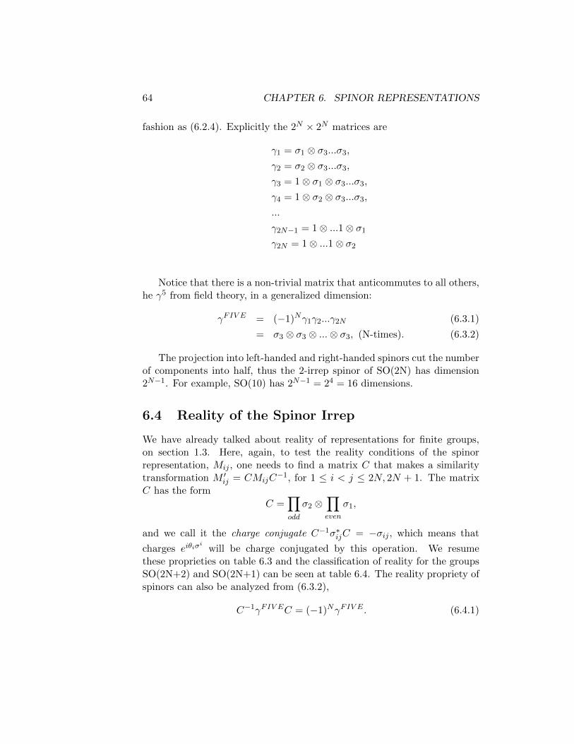
fashion as (6.2.4). Explicitly the 2N × 2N matrices are
γ1 = σ1 ⊗ σ3...σ3,
γ2 = σ2 ⊗ σ3...σ3,
γ3 = 1⊗ σ1 ⊗ σ3...σ3,
γ4 = 1⊗ σ2 ⊗ σ3...σ3,
...
γ2N−1 = 1⊗ ...1⊗ σ1
γ2N = 1⊗ ...1⊗ σ2
Notice that there is a non-trivial matrix that anticommutes to all others,he γ5 from field theory, in a generalized dimension:
γFIV E = (−1)Nγ1γ2...γ2N (6.3.1)
= σ3 ⊗ σ3 ⊗ ...⊗ σ3, (N-times). (6.3.2)
The projection into left-handed and right-handed spinors cut the numberof components into half, thus the 2-irrep spinor of SO(2N) has dimension2N−1. For example, SO(10) has 2N−1 = 24 = 16 dimensions.
6.4 Reality of the Spinor Irrep
We have already talked about reality of representations for finite groups,on section 1.3. Here, again, to test the reality conditions of the spinorrepresentation, Mij , one needs to find a matrix C that makes a similaritytransformation M ′ij = CMijC
−1, for 1 ≤ i < j ≤ 2N, 2N + 1. The matrixC has the form
C =∏odd
σ2 ⊗∏even
σ1,
and we call it the charge conjugate C−1σ∗ijC = −σij , which means that
charges eiθiσi
will be charge conjugated by this operation. We resumethese proprieties on table 6.3 and the classification of reality for the groupsSO(2N+2) and SO(2N+1) can be seen at table 6.4. The reality propriety ofspinors can also be analyzed from (6.3.2),
C−1γFIV EC = (−1)NγFIV E . (6.4.1)

6.4. REALITY OF THE SPINOR IRREP 65
(Mij)∗ = CMijC
−1 Hermitian Tα satisfies Mij
CT = (−1)N(N+1)
2 CReal symmetric C = CT ,
Pseudo-real anti-symmetric C = −CT(Mij)
∗ 6= CMijC−1 No Mij solutions, S interchanges to S
2n+ 2, n even: complex irrep, S, S.
Table 6.3: The definition for reality of spinor irrep for the orthogonal group.
SO(2 + 8k) complexSO(3 + 8k) pseudorealSO(4 + 8k) pseudorealSO(5 + 8k) pseudorealSO(6 + 8k) complexSO(7 + 8k) realSO(8 + 8k) realSO(9 + 8k) realSO(10 + 8k) complex
Table 6.4: The classification of reality of spinor irrep for the orthogonalgroup.
66 CHAPTER 6. SPINOR REPRESENTATIONS
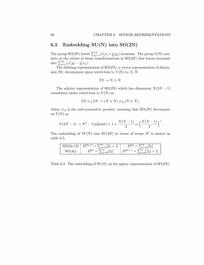
6.5 Embedding SU(N) into SO(2N)
The group SO(2N) leaves∑N
j=1(x′jxj+y′jyj) invariant. The group U(N) con-
sists on the subset of those transformations in SO(2N) that leaves invariantalso
∑Nj=1(x′jyj − y′jxj).
The defining representation of SO(2N), a vector representation of dimen-sion 2N, decomposes upon restriction to U(N) to N, N :
2N → N ⊕ N .
The adjoint representation of SO(2N) which has dimension N(2N − 1)transforms under restriction to U(N) as
2N ⊗A 2N → (N ⊕ N)⊗A (N ⊕ N),
where ⊗A is the anti-symmetric product, meaning that SO(2N) decomposeon U(N) as
N(2N − 1)→ N2 − 1(adjoint)⊕ 1⊕ N(N − 1)
2⊕(N(N − 1)
2
)∗.
The embedding of SU(N) into SU(2N) in terms of irreps Di is shown ontable 6.5.
SO(2n+2) D2n+1 =∑n
j=0[2j + 1] D2n =∑n
j=0[2j]
SO(4n) D2n =∑n
j=0[2j] D2n−1 =∑n−1
j=0 [2j + 1]
Table 6.5: The embedding of SU(N) on the spinor representation of SO(2N).

Chapter 7
Sp(2N), the Cn series
The symplectic groups, Sp(2N), are formed by matrices M that transformsas
Ω = MΩMT (7.0.1)
MΩ + ΩMT = 0, (7.0.2)
where
Ω =
(0 1−1 0
).
The rank of Sp(2N) is N and it has 2N2 + N generators. The sub-group USp(2N) is a simple and compact group formed by the intersectionof SU(2N) and Sp(2N,C), i.e. the compact form of Sp(2N),
USp(2N) = SU(N) ∪ Sp(2N).
From SU(N) we automatically get the additional condition to (7.0.2)condition M †M = −M . The general form of M of USp(2N) is composed bythe algebra of S(N),
Mij = Ai ⊗ I +3∑j=1
iSj ⊗ σj .
If Ai is real, M is anti-symmetric, otherwise, if Sj is real, M is symmet-ric. The number of non-compact generators minus the number of compactgenerator equal to the rank of the Lie algebra, therefore we can decomposeit as
M = (A⊗ I + S2 ⊗ iσ2) + (S1 ⊗ iσ1 + S3 ⊗ iσ3).
67

68 CHAPTER 7. SP(2N), THE CN SERIES
7.1 The Cartan Generators H
The first N-1 generators are the same Cartan subalgebra of SU(N) in thefirst block and its complex conjugate on the second (charge conjugation, soall weights change sign),
H1 =1
2
1 ...−1
0−1
10
2N×2N
,
H2 =1
2
1 ...1−2
0−1
−12
0
2N×2N
,
...
HN−1 =1√
2N(N − 1)
1 ...1
1−(N − 1)
−1−1
−1(N − 1)
2N×2N
,
The Nth Cartan generator is given by
HN =1√
2N(N − 1)
(1 00 −1
)2N×2N
.

7.2. THE WEIGHTS µ 69
7.2 The Weights µ
The 2N weights of the defining representation of USp(2N) are
µ1 =
(1
2,
1
2√
3,
1√24, ...,
1√2(N − 1)N
,1√2N
),
µ2 =
(− 1
2,
1
2√
3,
1√24, ...,
1√2(N − 1)N
,1√2N
),
µ3 =
(0,− 2
2√
12,
1√24, ...,
1√2(N − 1)N
,1√2N
),
...
µN−1 =
(0, 0, ..., 0,
N − 1√2(N − 2)(N − 1)
, ...
),
µN =
(0, 0, ..., 0,− N − 1√
2N(N − 1),
1√2N
),
µN+1 = −µ1,
...
µ2N = −µN .
7.3 The Raising and Lowering Operators E±
For j < k, one construct the raising operators of USp(2N),
E1,2 =
1 0 0 00 0 0 00 0 0 00 0 −1 0
,
E1,3 =
0 1 0 00 0 0 00 0 0 00 0 −1 0
2N×2N
,
E2,3 =
0 0 0 00 1 0 00 0 −1 00 0 0 0
2N×2N
,

70 CHAPTER 7. SP(2N), THE CN SERIES
...
E1,2+N =
0 0 1 00 0 0 00 0 0 00 0 0 0
2N×2N
,
E1,3+N =
0 0 0 10 0 1 00 0 0 00 0 0 0
2N×2N
,
E2,3+N =
0 0 0 00 0 0 10 0 0 00 0 0 0
2N×2N
,
...
The lowering operators are given by (Eij)† = −E−ij . The commutation
relation
[HI , Eα] = αIEα,
[HI , Eα] = (HI,jj −HI,kk)Ejk,
shows that Eα are eigenvalues of the H matrices.
7.4 The Roots α
The roots from the raising and lowering operators are give by αj,k = µj−µkand αj,k+N = µj + µk,
±(µi − µj), 1 ≤ i < j ≤ N,±(µi + µj), 1 ≤ i, j ≤ N.
Positive Roots
The positive roots are defined as the first positive entry from the right
µi − µj , i < j,
µi + µj , ∀ i , j .

7.5. THE FUNDAMENTAL WEIGHTS Q 71
Simple Roots
The N simple roots of USp(2N) are given by
α1 = (1, 0, 0, ..., 0),
α2 = (1
2,
√3
2, 0, ..., 0),
...
αN−1 = (0, ..., 0,− N − 2√2(N − 2)(N − 1)
,N√
2N(N − 1)),
αN = (0, ..., 0,− 2(N − 2)√2N(N − 1)
,
√2
N).
7.5 The Fundamental Weights q
The N fundamental weights are
q1 = (1
2,
1
2√
3, ...,
1√2N
),
...
qN−1 = (0, 0, ..., 0,
√N − 1
2N,N − 1√
2N),
qN = (0, 0, ..., 0,
√N
2).
7.6 The Cartan Matrix
The Cartan matrices identifies the family Cn,
A =
2 −1 0 0 ... 0 0 0−1 2 −1 0 ... 0 0 00 −1 2 −1 ... 0 0 00 0 −1 2 ... 2 −1 00 0 0 −1 ... −1 2 −10 0 0 0 ... 0 −2 2
.

72 CHAPTER 7. SP(2N), THE CN SERIES

Chapter 8
Young Tableaux
On the Young tableaux theory, each tableau represents a specific process ofsymmetrization and anti-symmetrization of a tensor v12...n in which index ncan take any integer value 1 to N.
For instance, lets us recall the defining representation of SU(N), com-posed of N-dimensional vectors vµ (it represents the usual vectors |µ〉, µ =1, ..., N). The tensor product is uµ ⊗ vν , with N2 components, is
δ(uµvν) = T νµ′uµ′vν + uµTµν′v
ν′ .
This tensor product forms irreps, i.e the. uµ⊗vν is reducible into irreps,and in the case that the representations are identical, the product space canbe separated into two parts, a symmetric and antisymmetric part,
uµ ⊗ vν =1
2(uµvν + uµvν)⊕ 1
2(uµvν − uνvµ). (8.0.1)
The decomposition of the fundamental representation specifies how asubgroup H is embedded in the general group G, and since all representa-tions may be built up as products of the fundamental representation, oncewe know the fundamental representation decomposition, we know all therepresentation decompositions.
The Young tableaux are then the box-tensors with N indices, where firstone symmetrizes indices in each row, and second one antisymmetrizes allindices in the collums. For example, we can construct the Young diagrams,from (8.0.1), for the tensorial product uµvν → µ ⊗ ν as
µ ⊗ ν = µ ν +
µν = tµν + tνµ
73

74 CHAPTER 8. YOUNG TABLEAUX
Another example, for N > 2, we have the tensor tµρν = vµ ⊗ uρ ⊗ hν ,and one writes
tµνρ −→ ( µ ⊗ ν ) ⊗ ρ =
( µ ν ⊕µν ) ⊗ ρ =
µ ν ρ ⊕µ ρν ⊕
µ νρ ⊕
µνρ
where, for example,
tµρν −→ν ρµ → (tµνρ + tµρν)− (tνµρ + tνρµ).
A third example, for N > 4, one can have a tensor of the form tµνργη,which will be generalized as
µ ⊗ ν ⊗ ρ ⊗ γ ⊗ η = ⊕ ... ⊕
Direct Products of two Irreps
The formal calculation of the direct product of two (or more) irreps is givenby the following rules:
1. On the second tensor in the tensorial multiplication, add to all boxesof the first row a indices, add to all boxes of the second row b indices,
etc. For example,
a ab .
2. The process of multiplication is made adding one box of index a eachtime to the others boxes, in all allowed ways, until ceasing these boxes.Then adding one box of index b each time to all, etc. Never put morethan one a or b in the same column. Align the number of a’s ≤ numberof b’s (at any position, number of a above and right must be equal orsmaller than of b, which must be equal or smaller than c, etc). For
example, a a b is not allowed.

75
3. If two tableaux of the same shape are produced, they are counted asdifferent only if the labels are different.
4. Cancel columns with N boxes since they are the trivial representation.
5. Check the dimension of the products to the dimension of the initialtensors.
Example vµν ⊗ uρ
b b ⊗ a = b b a +
b ba
Example uρ ⊗ vµν
The last one of this product is forbidden:
b ⊗ a a = b a a +
b aa +
baa
Example vµ ⊗ uνρThe first three of this product are forbidden:
c ⊗ab = ( c a +
ca ) ⊗ b
= c a b +
c ba +
c ba +
cab
Example vµν ⊗ uρλ
c c ⊗ab = ( c a +
c ca ) ⊗ b
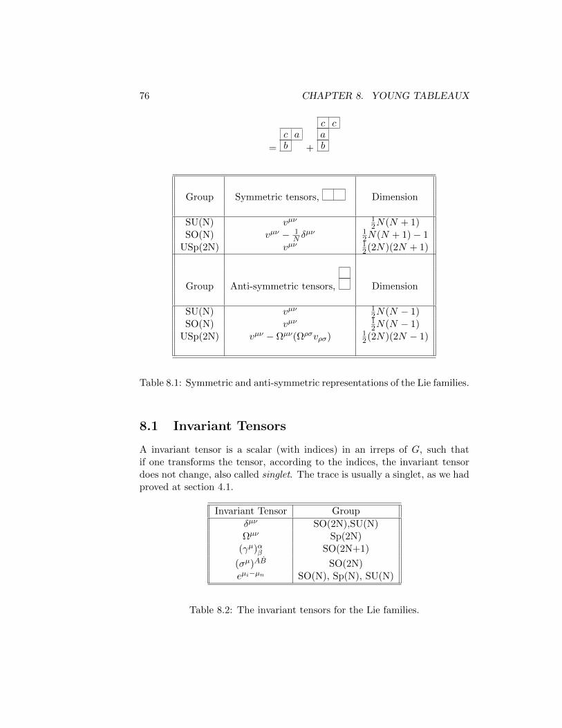
76 CHAPTER 8. YOUNG TABLEAUX
=
c ab +
c cab
Group Symmetric tensors, Dimension
SU(N) vµν 12N(N + 1)
SO(N) vµν − 1N δ
µν 12N(N + 1)− 1
USp(2N) vµν 12(2N)(2N + 1)
Group Anti-symmetric tensors, Dimension
SU(N) vµν 12N(N − 1)
SO(N) vµν 12N(N − 1)
USp(2N) vµν − Ωµν(Ωρσvρσ) 12(2N)(2N − 1)
Table 8.1: Symmetric and anti-symmetric representations of the Lie families.
8.1 Invariant Tensors
A invariant tensor is a scalar (with indices) in an irreps of G, such thatif one transforms the tensor, according to the indices, the invariant tensordoes not change, also called singlet. The trace is usually a singlet, as we hadproved at section 4.1.
Invariant Tensor Group
δµν SO(2N),SU(N)Ωµν Sp(2N)
(γµ)αβ SO(2N+1)
(σµ)AB SO(2N)eµi−µn SO(N), Sp(N), SU(N)
Table 8.2: The invariant tensors for the Lie families.

8.2. DIMENSIONS OF IRREPS OF SU(N) 77
For SO(2N), one can write the symmetric tensor tµν as u(µvν)− 1N δ
µνuv,where it was subtracted the trace, with dimension 1
2N(N + 1) − 1. Forthe antisymmetric part, the trace is not subtracted and the dimension is12N(N − 1). For the symplectic group Sp(2N), one writes an antisymmetricvector as uµvν − uνuµ − 2
NΩµνuv, which dimension is 12(2N)(2N − 1).
For example, the multiplication in SU(5) of 5 and 10 is given by thetensor tijk = φkη
ij . We separate out the trace φkηkj which transforms as 5
and we get 5⊗ 10 = 5⊕ 45.Another example the multiplication of 10 and 10, T ijmnh, taking the trace
and separate it out, T ijmij is 5, and the traceless, T ijmnj is 45. Therefore10⊗ 10 = 5⊕ 45⊕ 55.
A third example is for Usp(4), where one can decompose the tensorproduct of two vectors as
uµvν =uµvν + uνuµ
2+ [uµvν − uνvµ − 1
4Ωνµ(Ωρσu
ρvσ)],
where the last part is the trace. The tableaux representation is
⊗ = + + •.
8.2 Dimensions of Irreps of SU(N)
The general formula to calculate the dimension of irreps of SU(N) is givenby Dimension = Factors/Hooks, where factors are the terms inside theboxes and hook is the product of number of boxes in each hook. The di-mensions of the simplest representations are
dim( ) = N, fundamental representation of vµ,
dim( ⊗ ) = + = N2
dim( ) = 12N(N + 1), symmetric representation,
dim( )= 12N(N − 1), anti-symmetric representation,
dim( ⊗ ⊗ ) = +2 + = N3,
dim ( ) =
(N + 2
3
)=N(N + 1)(N + 2)
3!,

78 CHAPTER 8. YOUNG TABLEAUX
dim ( ) =
(N3
)=N(N − 1)(N − 2)
3!,
dim( ) = N3 − N(N+1)(N+2)3! − N(N−1)(N−2)
3! = 2N3
3 −2N3 .
For example, for SU(3), one has dim ( ) = 3, represented by vµ,
and dim ( × ) = 32, represented by uµν . For SU(6), dim ( ) = 6,represented by wµ.
The adjoint representation is the one with N − 1 boxes on first columnand only one box on second collumn. The complex conjugate of a irrep canbe found by replacing the j-column element by the N − j, and reading fromright. For example, for SU(3), one has
( )∗ = ( ).
For SU(4), one has
• ( )∗ = ,
• ( )∗ = ,
• ( )∗ = ,
• ( )∗ = ,
The Tensor Representation for SU(N)
The relation between the Young tableaux, the tensors of the group SU(N)and the fundamental weight is given by

8.3. DIMENSIONS OF IRREPS OF SO(2N) 79
µ −→ vµ, µ = 1, ..., N , ~q1 = µ1
12 −→ vµν = −vνµ, ~q2 = µ1 + µ2.
123 −→ vµνρ, ~q3 = µ1 + µ2 + µ3.
...
−→ ~qN−1 = µ1 + ...+ µN−1 = ( )∗
−→ For N boxes, this is a scalar.
When it comes to the complex representation, the highest weight of∗ is the lowest weight of ,
( )∗ = −µN ,= µ1 + ...+ µN−1,
= qN−1.
If the highest weight of two representations are vi, v2, the highest weight ofthe product of these representations are v1 + v2.
8.3 Dimensions of Irreps of SO(2N)
To count the dimension of a irrep on SO(2N), we write the Young tableauand fill it with the values of ri, λi (number of box in the i row, countingfrom N-1, N-2,...), λi (number of boxes forming a column on the i row), andRi (sum of ri and λi), as shown on table 8.3.

80 CHAPTER 8. YOUNG TABLEAUX
ri (rows) λi (columns) Ri = ri + λi
N-1 +2 N-1 +2
N-2 +2 N-2 +2
... +2 ... +2
1 +1 20 0 0
Table 8.3: Calculation of the dimension of irreps on SO(2N).
The dimension of the tensors (without spinors) is then calculated by mul-tiplying all possible sums of Ri, multiplying all possible differences betweenthem and dividing by all possible sums of ri times and their differences,
dimension =
∏Sums (Ri +Rj)∏Sums (ri + rj)
∏Differences (Ri −Rj)∏Differences (ri − rj)
.
For spinors one just needs to make Ri = ri + λi + 12 .
Example: SO(6)
Let us calculate an irrep on SO(6). For instance, the multiplication of twovectors can be written as
vµ ⊗ tν = vµtν + vνtµ − 2
Ngµνvt. (8.3.1)
Considering first of all the symmetrical part, one has the table 8.4.
ri (rows) λi (columns) Ri = ri + λi
2 2 41 0 10 0 0
Table 8.4: Example of counting dimensions for a symmetric irrep on SO(6).
dimension =5.4.1× 3.4.1
3.2.1× 1× 2.1= 20.

8.4. DIMENSIONS OF IRREPS OF SO(2N+1) 81
ri (rows) λi (columns) Ri = ri + λi
2 1 3
1 1 20 0 0
Table 8.5: Example of counting dimensions for an anti-symmetric irrep onSO(6).
We then consider the anti-symmetric part, as shown on table 8.5.
dimension =5.3.1× 1.3.2
3.2.1× 1× 2.1= 15.
The dimension of the tensorial product given by (8.3.1) is clearly 20+15+1,where this last part is the trace. Now, let us consider the the dimension ofspinor representation on SO(6), placing a dot inside the tableaux, as ontable 8.6.
ri (rows) λi (columns) Ri = ri + λi
2 . 1 3 12
1 0 112
0 0 12
Table 8.6: Example of counting dimensions for a irrep on SO(6) with spinorrepresentation.
dimension =5.4.2× 2.3.1
3.2.1× 1× 2.1= 20.
8.4 Dimensions of Irreps of SO(2N+1)
Already including spinors (Ri = ri + λi + 12) one can count the dimensions
of the irreps with the following rules of table 8.7.
The dimension for the tensor are then again the multiplication of sumsand differences of Ri over the multiplication of sum and differences of ri,
dimension =
∏Sums (Ri +Rj)∏Sums (ri + rj)
∏Differences (Ri −Rj)∏Differences (ri − rj)
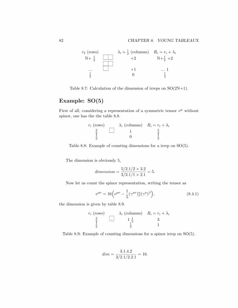
82 CHAPTER 8. YOUNG TABLEAUX
r2 (rows) λi + 12 (columns) Ri = ri + λi
N+ 12 +2 N+1
2 +2
... +1 ... 112 0 1
2
Table 8.7: Calculation of the dimension of irreps on SO(2N+1).
Example: SO(5)
First of all, considering a representation of a symmetric tensor vµ withoutspinor, one has the the table 8.8.
ri (rows) λi (columns) Ri = ri + λi32 1 5
212 0 1
2
Table 8.8: Example of counting dimensions for a irrep on SO(5).
The dimension is obviously 5,
dimension =5/2.1/2× 3.2
3/2.1/1× 2.1= 5.
Now let us count the spinor representation, writing the tensor as
vµν = 16(vµν − 1
5(γµν)αβ(γµ)β
), (8.4.1)
the dimension is given by table 8.9.
ri (rows) λi (columns) Ri = ri + λi32
. 1 12 3
12
12 1
Table 8.9: Example of counting dimensions for a spinor irrep on SO(5).
dim =3.1.4.2
3/2.1/2.2.1= 16.

8.5. DIMENSIONS OF IRREPS OF SP(2N) 83
8.5 Dimensions of Irreps of Sp(2N)
The calculation of the dimension of irreps of Sp(2N) is slightly different fromthe previous process for the orthogonal group. Again one needs to fill theri, λi and Ri, as it is shown on table 8.10.
r2 (rows) λi + 12 (columns) Ri = ri + λi
N +2 N +2
... +2 ...+2
1 0 1
Table 8.10: Example of counting dimensions for a irrep on Sp(2N).
The dimension for the tensors is then given by the multiplication of allsums of Ri, all differences of Ri and (this is different) the multiplication ofall Ri, all over the double factorial on (2N − 1)!!.
dimension =
∏Sums (Ri +Rj)
∏Differences (Ri +Rj)
∏Ri
1!3!...(2N − 1)!!
It is useful to check the local isomorphism of USp(4) ' SO(5), which isclearly seen by their Young tableaux, table 8.11.
Tableau Dimension
4
10
5
16
Table 8.11: Young tableaux from the local isomorphism SU(5) ' USp(4).
8.6 Branching Rules
Restricted representation is a construction that forms a representation ofa subgroup from a representation of the whole group. The rules for de-

84 CHAPTER 8. YOUNG TABLEAUX
composing the restriction of an irreducible representation into irreduciblerepresentations of the subgroup are called branching rules. In the case ofSU(N) groups, one can decompose it as
SU(N)→ SU(M)× SU(N −M)× U(1),
where the first two are represented by the diagonal matrix(SU(M) 0
0 SU(N −M)
),
and the extra U(1) is embedded as(diag 1
M 00 diag − 1
M−N
).
The splitting in the Dynkin diagram is obtained by deleting one node,the one that connects SU(M) to SU(N-M). For example, for
SU(8)→ SU(4)× SU(4)× U(1),
the fundamental representation is
N ' M ⊕ N−M .

Chapter 9
The Gauge Group SU(5) as asimple GUT
The idea of the Grand Unified Theories (GUTs) is to embed the StandardModel (SM) gauge groups into a large group G and try to interpret theadditional resultant symmetries. Currently the most interesting candidatesfor G are SU(5), SO(10), E6 and the semi-simple SU(3)× SU(3)× SU(3).Since the SM group is rank 4, all G must be at least rank N − 1 = 4 andthey also must comport complex representations. The SU(5) grand unifiedmodel of Georgi and Glashow is the simplest and one of the first attemptsin which the SM gauge groups SU(3) × SU(2) × U(1) are combined intoa single gauge group, SU(5). The Georgi-Glashow model combines leptonsand quarks into single irreducible representations, therefore they might haveinteractions that do not conserve the baryon number, still conserving thedifference between the baryon and the lepton number (B-L). This allows thepossibility of proton decay whose rate may be predicted from the dynam-ics of the model. Experimentally, however, the non-observed proton decayresults on contradictions of this simple model, still allowing however super-symmetric extensions of it. In this paper I tried to be very explicit in thederivations of SU(5) as a simple GUT.
9.1 The Representation of the Standard Model
The current theory of the electroweak and strong interactions is based on thegroup SU(3)×SU(2)×UY (1), henceforth called the Standard Model of Ele-mentary particles. This theory states that there is a spontaneous symmetrybreaking (SSB) at around 100 GeV, breaking SU(2)×UY (1)→ UEM (1) via
85

86 CHAPTER 9. THE GAUGE GROUP SU(5) AS A SIMPLE GUT
the Higgs mechanism. In the SM, the three generations of quarks are threeidentical copies of SU(3) triplet and the right-handed (RH) antiparticles (orleft-handed (LH) particles) are SU(2) doublet. The remaining particles aresinglet under both symmetries. For the first generation, the RH antiparticlesSU(2) doublet are 12
ψ† =
(ud
), l† =
(eνe
).
The representation of the RH antiparticle creation operators can be seenin table 9.1. For the LH particle creation one just takes the complex con-jugate of RH, where for SU(2), 2 = 2, since SU(2) is pseudo-real. Theresultant operators are shown in table 9.2.
Creation Op. Dim on SU(3) Dim on SU(2) Y of U(1) Representation
u† Triplet Singlet 23 u† : (3, 1)2/3
d† Triplet Singlet −13 d† : (3, 1)−1/3
e† Singlet Singlet −1 e† : (1, 1)−1
ψ† Triplet Doublet −16 ψ† : (3, 2)−1/6
l† Singlet Doublet 12 l† : (1, 2)1/2
Table 9.1: The representations of the right-handed antiparticle creation op-erators of the standard model, SU(3) × SU(2) × U(1). ”Dim” stands fordimension, Y is the hypercharge of the U(1) generators S.
The full SU(3)× SU(2)× U(1) RH representation of the creation oper-ators is then
u† ⊕ d† ⊕ e† ⊕ ψ† ⊕ l† = (9.1.1)
(3, 1)2/3 ⊕ (3, 1)−1/3 ⊕ (1, 1)−1 ⊕ (3, 2)−1/6 ⊕ (1, 2)1/2. (9.1.2)
The full SU(3)× SU(2)× U(1) LH representation of the creation oper-ators is then
u† ⊕ d† ⊕ e† ⊕ ψ† ⊕ l† = (9.1.3)
(3, 1)−2/3 ⊕ (3, 1)1/3 ⊕ (1, 1)1 ⊕ (3, 2)1/6 ⊕ (1, 2)−1/2. (9.1.4)
1RH neutrinos weren’t experimentally observed. It is possible to have only LH neu-trinos without RH neutrinos if we could introduce a tiny Majorana coupling for the LHneutrinos.
2For the antiparticle of the electron, the positron, for convenience we write in this texte+ = e.

9.2. SU(5) UNIFICATION OF SU(3)× SU(2)× U(1) 87
Creation Op. Dim on SU(3) Dim on SU(2) Y of U(1) Representation
u† Triplet Singlet −23 u† : (3, 1)−2/3
d† Triplet Singlet 13 d† : (3, 1)1/3
e† Singlet Singlet 1 e† : (1, 1)1
ψ† Triplet Doublet 16 ψ† : (3, 2)1/6
l† Singlet Doublet −12 l† : (1, 2)−1/2
Table 9.2: The representations of the left-handed particle creation operatorsof the standard model, SU(3)×SU(2)×U(1). ”Dim” stands for dimension,Y is the hypercharge of the U(1) generators S.
The standard similar way of writing the representations of (LH) matteras representations of SU(3)× SU(2) in the SM is
(u, d) : (3,2); (νe, e−) : (1,2); (uc, dc) : (3,2); (e+) : (1,1). (9.1.5)
9.2 SU(5) Unification of SU(3)× SU(2)× U(1)The breaking of SU(5) into SU(3)×SU(2)×U(1) can be done in the samefashion as the breaking of SU(3) into SU(2) × U(1). The SU(5) breakingoccurs when a scalar field (such as the Higgs field) transforming in its adjoint(dimension N2−1 = 52−1 = 24) acquires a vacuum expectation value (VEV)proportional to the hypercharge generator,
S =Y
2=
−1
3−1
3−1
312
12
. (9.2.1)
These 24 gauge bosons are the double than the usual 12. The additionalgauge bosons are called X and Y and they violate the baryon and leptonnumber and carry both flavor and color. As a consequence, the proton candecay into a positron and a neutral pion3, with a lifetimes given by
τp ∼1
α2su(5)
M4X
m5p
.
3As we see on the last section of the text, no such decay was observed.

88 CHAPTER 9. THE GAUGE GROUP SU(5) AS A SIMPLE GUT
The SU(5) is then spontaneously broken to subgroups of SU(5) plusU(1) (the abelian group representing the phase from (9.2.1)). This SSB canbe represented as 5⊕10⊕1 to LH particles and 5⊕10⊕1 to RH antiparticles,as we will prove in the following sections.
Unbroken SU(5)
The fundamental representation of SU(5), let us say the vectorial repre-sentation |ε1ε2ε3ε4ε5〉, has dimension N=54. The group is complex havingan anti-fundamental representation (complex conjugate representation) 5.The embedding of the standard gauge groups in SU(5) consists in findinga SU(3)× SU(2)× U(1) subgroup of SU(5). We first look to 5 and try tofit a 5-dimensional subset of (9.1.2) on it (and the left-handed (9.1.4) on 5).There is two possibilities on (9.1.2) that sum up 5 dimensions:
(3, 1)−1/3 ⊕ (1, 2)1/2, (9.2.2)
and
(3, 1)2/3 ⊕ (1, 2)1/2.
The second one is not allowed because S, the generator of U(1), willnot be traceless5, therefore this group can not be embed in SU(5) in thiscase. To verify it just do 2
3 × 3 + 12 × 2 6= 0 (not traceless), differently of
−13 × 3 + 1
2 × 2 = 0 (traceless).The first possibility, (9.2.2) is allowed and represents the embedding.
The SU(3) generators, Ta, act on the first indices of the fundamental rep ofSU(5) |ε1ε2ε300〉 and the SU(2) generators, Ra, act on the last two |000ε4ε5〉.The U(1) generator, S, obviously commutes with the other generators. Theembedding of the first RH subset of fermions on SU(5) is then characterizedby the traceless generators(
Ta 00 0
)5×5
,
(0 00 Ra
)5×5
,
(− I
3 0
0 I2
)5×5
.
In the same logic, the embedding of the LH subset of fermions on SU(5)is characterized by the traceless generators(
Ta 00 0
)5×5
,
(0 00 Ra
)5×5
,
(I3 0
0 − I2
)5×5
.
4See construction of the Lie groups on reference [?].5All generators of SU(N) are traceless for definition and construction.

9.2. SU(5) UNIFICATION OF SU(3)× SU(2)× U(1) 89
ψi 5→ (3, 1)−1/3 ⊕ (1, 2)1/2 uc, l(ec, νce)
ψi 5→ (3, 1)1/3 ⊕ (1, 2)−1/2 dc, l(e, νe)
Table 9.3: The SU(3)× SU(2)× U(1) embedding on the fundamental rep-resentation of SU(5). The index c indicates charge conjugation.
A possible representation of the LH 5, rewriting |ε1ε2ε3ε4ε5〉6 is7dcreddcbluedcgreeneνe
c
=
(dc3l2
)5
,
and as the RH, given by 5,ucreducblueucgreeneνe
c
=
(uc3l2
)5
.
The next representation on SU(5) we will use is the antisymmetric intwo indices, 10 and its conjugate 10. The remaining ten-dimensional partof (9.1.2) and (9.1.4) fits respectively on 10 and 10. To see how it happens,we observe that 10 = 5 ⊗A 5 so we can multiply the 5-dimensional subsetson table 9.3 to form these representations. For instance, the LH particles(9.1.4) subset forms[(3, 1) 1
3⊕ (1, 2)− 1
2
]⊗A
[(3, 1) 1
3⊕ (1, 2)− 1
2
]= (6, 1) 2
3⊕ (−3, 1) 2
3⊕ (3, 2)− 1
6⊕ (1, 3)−1 ⊕ (1,−2)−1,
= (3, 1) 23⊕ (3, 2)− 1
6⊕ (1, 1)−1.
where we have used 3 ⊗ 3 = 3 ⊕ 6 and 2 ⊗ 2 = 1 ⊕ 3 and ⊗A is theantisymmetric product (the first of each part).
Finally, all the remaining fermions transforming as a singlet (1) underSU(5)8. The final embedding of fermions of the standard model into thegauge group SU(5) is shown on table 9.5.
6The index c indicates charge conjugation.7Here we ignore the Cabibo type mixing.8This is necessary because of the evidence for neutrino oscillations.

90 CHAPTER 9. THE GAUGE GROUP SU(5) AS A SIMPLE GUT
10→ (3, 2)1/6 ⊕ (3, 1)−2/3 q, uc, ec
10→ (3, 2)−1/6 ⊕ (3, 1)2/3 q, dc, e
Table 9.4: The SU(3) × SU(2) × U(1) embedding on the anti-symmetricrepresentation 10 of SU(5).
SU(5) Decomposition Fermions Similar Notation
ψi 5→ (3, 1)−1/3 ⊕ (1, 2)1/2 uc, l(ec, νce) (3,1,-1/3) + (1,2,1/2)
ψij 10→ (3, 2)−1/6 ⊕ (3, 1)2/3 u, dc, e (3,1,2/3) + (3,2,-1/6)+(1,1,1)
• 1→ (1, 1)0 νc
ψi 5→ (3, 1)1/3 ⊕ (1, 2)−1/2 dc, l(e, νe) (3,1,1/3) + (1,2,-1/2)
ψij 10→ (3, 2)1/6 ⊕ (3, 1)−2/3 d, uc, ec (3,1,-2/3) + (3,2,1/6)+(1,1,1)
• 1→ (1, 1)0 νc
Table 9.5: The 5 ⊕ 10 ⊕ 1, LH particles, and 5 ⊕ 10 ⊕ 1, RH antiparticles,embedding of SM on SU(5).

9.2. SU(5) UNIFICATION OF SU(3)× SU(2)× U(1) 91
Breaking SU(5)
The gauge bosons of the model are given by the adjoint 24 of SU(5), trans-forming as
24→ (8, 1)0 ⊕ (1, 3)0 ⊕ (1, 1)0 ⊕ (3, 2)−5/6 ⊕ (3, 2)5/6, (9.2.3)
described in detail in table 9.6.
SM GB Add. SU(3) Add. SU(2) Identification
(8, 1)0 (8,1,0) X - - Gαβ(1, 3)0 (1,3,0) X - - W±,W 0
(1, 1)0 (1,1,0) X - - B(3, 2)−5/6 (3,2,-5/6) - Triplet Doublet Aτα = (Xα, Yα)
(3, 2)5/6 (3,2,5/6) - Triplet Doublet Aατ = (Xα, Yα)T
Table 9.6: The gauge bosons of SM fitting on the adjoint representation ofSU(5). SM stands for standard model, ”Add” stands for additional, andGB for gauge boson.
As we already mentioned, the fermions have to acquire mass in SU(5)by a SSB, which also must happen in the GUT theory. For making thisto happen, the product of the representations containing the fermions andantifermions (table 9.5), must contain a component which transforms as theSU(3) × SU(2) × U(1) Higgs field, represented by (1, 2)1/2 and (1, 2)−1/2.It is easy to understand it because the particles and antiparticles of thefermions appears in both 5, 10 for RH (and 10, 5 for LH).
First, for the RH antiparticles, the product of these representations are
10⊗ 5 = ⊗ = ⊕ = 5⊕ 45From (9.2.2) we see that 5 contains (1, 2)1/2, it is also contained on 45,
therefore both representations can give mass to d, e. For the LH particles,the product of these representations are
10⊗ 10 = ⊗ = ⊕ ⊕ = 50⊕ 45⊕ 5.Again 5 and 45 contains (1, 2)−1/2, giving mass to u, however 50 does
not contain (1, 2)−1/2.

92 CHAPTER 9. THE GAUGE GROUP SU(5) AS A SIMPLE GUT
9.3 Anomalies
If the creation generator for all the right hand operators of spin-1/2 particlestransform according to a representation generated by TRa , we nee to have
tr[T aR, T bRT cR
]= 0. (9.3.1)
In fact it is true for all simple Lie algebra with exception of SU(N)for N ≤ 3. Therefore, the anomaly in any representation of SU(N) isproportional to
Dabc = tr[T aR, T bRT cR
]=
1
2A(R)dabc, (9.3.2)
where2dabcLc = La, Lb. (9.3.3)
A(R) is independent of the generators allowing us to choose one gener-ator and calculate it. In our case it is useful to use the generator as thecharge operator
Q = R3 + S, (9.3.4)
and looking at (9.2.1), one has
A(5)
A(10)=
tr Q3(ψi)
tr Q3(ψii)= −1. (9.3.5)
It is clear now that the fermions in these representations have theiranomalies canceled
A(5) +A(10) = 0. (9.3.6)
9.4 Physical Consequences of using SU(5) as a GUTTheory
• The charge of the quarks can be deduced from the fact that thereare three color states and from the fact that the charge operators is(9.3.4), Q = R3 +S = I3 + Y
2 , and it must be traceless. The multipletof the 5 representation gives
Q(νe) +Q(e) + 3Q(d) = 0→ Q(d) = −1
3Q(e),
which gives an answer to the charge quantization, not explained n theSM.
9.4. PHYSICAL CONSEQUENCES OF USING SU(5) AS AGUT THEORY93
• The Weinberg angle,
sin 2(θW ) =g′2
g2 + g′2,
g, g′ the coupling constants of gauge bosons in the electroweak theory,cannot be calculated on SM (it is a free parameter). In SU(5) GUT,however, the Weinberg angle is accurately predicted, giving sin2θW ∼0.21.
• If a group is simple then its GUT has only one coupling constant beforeSSB. The three coupling constants of the SM are energy dependent andin SU(5) they unit at ∼ 1015 GeV. However, a supersymmetric SU(5)is needed to get an exact unification in a single point. Rememberthat in the SM the strong, weak and electromagnetic fine structureconstants are not related in any fundamental way.
• No proton decay was observed, which is a contradiction to its lifetimeestimated in SU(5), (9.2.2). In a supersymmetric SU(5) the protonlifetime is longer, being apparently experimentally consistent.
• Finally, it is actually clear that the SU(5) might be incomplete whenone considers the fact that neutrinos were observed to carry smallmasses and there might exist extra RH Majorana neutrinos. As we justlearned, it is not possible to introduce RH neutrinos trivially in thissimple model. One solution is going to the next (complex) gauge groupSO(10), where the spinor representation can accommodate sixteen LHfields, or even to E6, which motivates string theories.
94 CHAPTER 9. THE GAUGE GROUP SU(5) AS A SIMPLE GUT

Chapter 10
Geometrical Proprieties ofGroups and Other NiceFeatures
10.1 Covering Groups
In defining representations of continuous groups, we require the matrixelements of the representation to be continuous functions on the groupmanifold. Among the continuous functions which are multi-valued thereare possibility of multiply valued representations. A representation of agroup G will be called an m-valued representation if m-different operationsD1(R), .., Dm(R) are associated with each elements of the group and allthese operations must be retained if the group is continuous. For all pos-sible closed curves of the manifold, looking to the values of some functionalong these curves, if on returning to the initial point we find m-differentvalues of the function, we say that the function is m-valued. A group issimple connected if every continuous function on the group is single valued,and it is m-connected if there are m closed curves which cannot be deformedinto one another, i.e. m-valued continuous functions can exist, some of theirreps of the manifold are m-valued.
For example, for the rotation group em two-dimensions, a function f(θ) =eiaθ is single valued if a is integer, t-valued if a is rational and multi-valuedif a is irrational. The difficult related to multiply valued function and irrepsis overcome by considering universal covering group.
A covering group of a topological group H is a covering space G of Hsuch that G is a topological group and the covering map f : G → H is a
95

96CHAPTER 10. GEOMETRICAL PROPRIETIES OF GROUPS ANDOTHER NICE FEATURES
continuous group homomorphism. The group H always contains a discreteinvariant subgroup N such that
G ' H/N.
From last example, the functions eiaθ will be single valued on H. Every irrepof G, single or multi-valued, is single valued on H (and then all definitionsof multiplication and the orthogonality theorems hold).
A double covering group is a topological double cover in which H has twoin G, and includes, for instance, the orthogonal group. If G is a coveringgroup of H then they are locally isomorphic1.
A universal covering group is always simple connected, any closed curvein this group can be shrunk or contracted to a point. If the group is alreadysimple connect, its universal covering group is itself. The universal cover isalways unique and always exist.
It easy to see that the rotation group SO(3) has as a universal cover thegroup SU(2)2 which is isomorphic to the group to Sp(2). The group SO(N)has a double cover which is the spin group Spin(N) and for N ≥ 3, the spingroup is the universal cover of SO(N). A closed curve contractible to a pointhas components in spinor representation that are single valued (a closedcurve that is not contractible to a point can be defined as double-valued).For N ≥ 2 the universal cover of the special linear group SL(N, R) is nota matrix group, i.e. it has no faithful finite-dimensional representations.Besides the fact that Sl(2,C) is simple connected, the group Gl(2,C) is notsimple connect, and one can see it remembering that Gl(2,C) = U(1)Sl(2,C),where the unitary group, which is only a phase, is infinitely connected.
For instance, the annulus and the torus are infinity connected. Thesphere (N > 1) is simple connected. The simple circumference S1 is infiniteconnected. The N-euclidian space is simple connected even when removingsome single points from space.
If one can set up a 1-1 continuous correspondence between the points oftwo spaces, then they have the same connectivity. For example, SN , N ≥2,∑N
i=1 x2i = 1, is simple connected since can use stereographic projection to
set a 1-1 correspondence with the (N − 1)-dimension euclidian space.
1The Lie algebra are isomorphic but the groups are locally isomorphic: the proprietiesof the groups are globally different but locally isomorphic.
2Any 2 × 2 hermitian traceless matrix can be written as X = ~x~σ. For any element Uof SU(2), X ′ = UXU† is hermitian and traceless so X ′ = ~x′~σ and tr X2 = tr X2. Thus~x rotate into ~x′ and we can associate a rotation to any U . Since U and −U are associatedto the same rotation, this gives a double covering of SO(3) by SU(2).

10.1. COVERING GROUPS 97
Example: Addition Group for S1 and R
Let us construct the sum of the infinitely connected group S1 and the lineR, which is simple connected,
• R: −∞ < x <∞.
• S1 : e2πix with 0 ≤ θ < 1.
The map is in the form R→ S1, which means x→ e2πiθ, which is the groupU(1). From this example, we resume covering group relation on table 10.1.
H → GH/N ' G
The kernel N lies in the center of H and its a invariant subgroup.
Table 10.1: Diagram for covering groups.
A trivial example is the case of SU(2), which center is diag(1,-1), this isexactly Z2.
Example: SU(2) ' S3
The elements of SU(2) are given by g,
g = ei2ωiσj = cos(
ω
2) +
iω
2sin
ω
2,
with proprieties g†g = 1 and det g = 1. All points at ω = 2π has to beidentified. The surface of B3 is a S2. One wraps it and the point in thebottom is identified as the superficies ω = 2π.
Isomorphism
It is a 1-1 mapping f of one group onto another, G1 → G2 , preserving themultiplication law. It has the same multiplication table. For example, everyfinite group is isomorphic to a permutation group. A relation of locallyisomorphic groups is shown on table 10.2.

98CHAPTER 10. GEOMETRICAL PROPRIETIES OF GROUPS ANDOTHER NICE FEATURES
SU(2) ' SO(3)SU(1, 1) ' SO(2, 1)
SU(2)× SU(2) ' SO(4)Sl(2, C) ' SO(3, 1)
SU(2)× Sl(2, 2) ' SO(4)∗
USP (4) ' SO(5)USP (2, 2) ' SO(4, 1)Sp(4, R) ' SO(3, 2)SU(4) ' SO(6)SU(4)∗ ' SO(5, 1)SU(2, 3)∗ ' SO(4, 2) (AdS/CFT)Sl(4, R) ' SO(3, 3)Sl(3, 1) ' SO(6)
Table 10.2: Table of covering groups for the Lie groups.
Homomorphism
It is a 1-1 mapping f to the same point, G → G′, preserving the metricstructure. The image f(G) forms a subgroup of G′, the kernel K forms asubgroup of G.
The first isomorphism theorem says that any homomorphism f(G) withkernel K is isomorphic to G/K. The kernel of a homorphism is an invariantsubgroup.
10.2 Invariant Integration
Groups can be seen as curved manifolds and the Haar measure is a way toassign an invariant volume to subsets of locally compact topological groupsand define an integral for functions on these groups. It possible to have ameasure when ∑
g∈Gf(g) =
∑g
f(g g),
and the left measure is then∫f(α)µL(α)dα =
∫f(β α)µL(α)dα. (10.2.1)

10.2. INVARIANT INTEGRATION 99
We want to associate to a set of elements in the neighborhood of aelement A a volume (measure) τA such that the measure of the elementsobtained from these elements by left translation with B is the same, dτA =dτBA.
The generalization of this for continuous groups is giving by writing theelements as g(α) = eα
µTµ . Clearly g(α)g(β) = g(α β), which is the groupcomposition law and it is exactly (10.2.1). In this representation, the unitaryelement e is g(0). The invariant integration has also the propriety of internaltranslation invariance,∫
f(x)dx =
∫f(x− q)dx.
The right invariant measure is given by∫g∈µ
f(α)µR(α)dα =
∫f(−β α)µR(α)dα.
For compact, for infinite and for discrete groups, µL = µR, the leftmeasure is equivalent to the right. A pragmatic way of finding the measureof a group is defining a density function ρ(a) such that
dτA = ρ(A)dA = ρ(BA)dAB = dτBA.
Isomorphic groups always have the same density function. In the neighbor-hood of the identity, we can make
dB = J(B)dA,
where J(B) is the jacobian, i.e. the left measure can be defined as thedeterminant of the matrix of all changes (the jacobian).
Trivial Examples
For the group g′ = a + g, one defines the function φ(a, b) = a + b. Thejacobian is given by
∂φ(a, b)
∂a
∣∣∣a=0
= 1.
Then J(b) = 1, ρ(b) = 1 and the measure is∫dbf(b).
For the group g′ = ag, one defines the function φ(a, b) = ab and
∂φ(a, b)
∂a
∣∣∣a=1
= b.
Then J(b) = b, ρ(b) = 1b and the measure is
∫1bdbf(b).

100CHAPTER 10. GEOMETRICAL PROPRIETIES OF GROUPS ANDOTHER NICE FEATURES
A Pathological Example3
For the group given by the representation element
g(α) =
(eα
1α2
0 1
).
one has, from g(β)g(α) = g(β α),
g(α)g(β) =
(eβ
1β2
0 1
).
(eα
1α2
0 1
)=
(eα
1+β1eβ
1α2 + β2
0 1
).
Writing as
ψ1(β, α) = β1 + α1,
ψ2(β, α) = eβ1α2 + β2,
we have (eψ
iψ2
0 1
).
The left measure is then given by
∂ψ1,2(β, α)
∂α2
∣∣∣α2=1,α1=0
= eβ1 → µL(β) = eβ
1,
the right measure is given by
∂ψ1,2(β, α)
∂α1
∣∣∣α2=0,α1=1
= 1→ µR(β) = 1.
Therefore we see that these two measures are different for this non semi-simple space.
Theorem: The left measure is equal to the right measure if the structureconstant of the Lie algebra has trace equal to zero fµµα = 0.
3Exercise proposed by Prof. van Nieuwenhuizen.

10.2. INVARIANT INTEGRATION 101
Invariant measure in Lie Groups
In SU(2) (also Sl(2,R), Sl(2,C) or Gl(2,R)), one has
g = a0 + aki σk = eiωiσi2 ,
where
σ20 +
∑σ2k = 1.
The Haar measure can then be written as∫f(α)µL(α)d1
αd2αd
3α.

102CHAPTER 10. GEOMETRICAL PROPRIETIES OF GROUPS ANDOTHER NICE FEATURES

Appendix A
Table of Groups
Group Name Dim Def irrep Section
Sn Symmetric group N, finite 1.4Zn, Cn Cyclic group N, finite 1.4An Alternating group N, finite 1.4D2N Dihedral group 2N, finite 1.4
U(N) Unitary group N, Infinite 3SU(N) Special Unitary group N, Infinite 3SO(2N) Special Orthogonal group 2N, Infinite 4Sp(2N) Symplectic group 2N, Infinite 7
GL(N,C) General Linear group N, Infinite 10.1SL(N,C) Special Linear group N, Infinite 10.1
Table A.1: Summary of groups.
103

104 APPENDIX A. TABLE OF GROUPS

List of Tables
1.1 Geometric objects related to their dimensions. . . . . . . . . . 17
2.1 Distinction among the elements of the group and the elementsof the representation (the generators), for Lie groups. . . . . . 20
2.2 Definition algebras in terms of ideals. . . . . . . . . . . . . . . 20
2.3 Number of generators for the compact and simple families onthe Lie Algebra. . . . . . . . . . . . . . . . . . . . . . . . . . 23
2.4 Local isomorphism among the Cartan families. . . . . . . . . 32
2.5 Order of the independent invariants for the four Lie families. 34
2.6 The Lie groups in terms of the compact and non-compactgenerators. . . . . . . . . . . . . . . . . . . . . . . . . . . . . 35
3.1 The decomposition of SU(N) into its irreps. . . . . . . . . . . 38
3.2 The highest weight of all irreps of SU(6). . . . . . . . . . . . 41
3.3 The generators, weights, simple root and fundamental weightof the defining representation of SU(2). . . . . . . . . . . . . . 43
3.4 The generators, weights, simple roots and fundamental weightsof the defining representation of SU(3). . . . . . . . . . . . . . 47
6.1 Example of spinor representation for SO(4), an euclidian spaceof dimension 4. This representation is pseudo-real, which isnot a surprise since SO(4) ' SU(2) ⊗ SU(2) and SU(2) ispseudo-real. . . . . . . . . . . . . . . . . . . . . . . . . . . . . 59
6.2 The Dirac group for dimensions 2, 3 and 4 (euclidian andminkowskian). . . . . . . . . . . . . . . . . . . . . . . . . . . . 61
6.3 The definition for reality of spinor irrep for the orthogonalgroup. . . . . . . . . . . . . . . . . . . . . . . . . . . . . . . . 65
6.4 The classification of reality of spinor irrep for the orthogonalgroup. . . . . . . . . . . . . . . . . . . . . . . . . . . . . . . . 65
105

106 LIST OF TABLES
6.5 The embedding of SU(N) on the spinor representation ofSO(2N). . . . . . . . . . . . . . . . . . . . . . . . . . . . . . . 66
8.1 Symmetric and anti-symmetric representations of the Lie fam-ilies. . . . . . . . . . . . . . . . . . . . . . . . . . . . . . . . . 76
8.2 The invariant tensors for the Lie families. . . . . . . . . . . . 768.3 Calculation of the dimension of irreps on SO(2N). . . . . . . 808.4 Example of counting dimensions for a symmetric irrep on SO(6). 808.5 Example of counting dimensions for an anti-symmetric irrep
on SO(6). . . . . . . . . . . . . . . . . . . . . . . . . . . . . . 818.6 Example of counting dimensions for a irrep on SO(6) with
spinor representation. . . . . . . . . . . . . . . . . . . . . . . 818.7 Calculation of the dimension of irreps on SO(2N+1). . . . . . 828.8 Example of counting dimensions for a irrep on SO(5). . . . . 828.9 Example of counting dimensions for a spinor irrep on SO(5). 828.10 Example of counting dimensions for a irrep on Sp(2N). . . . . 838.11 Young tableaux from the local isomorphism SU(5) ' USp(4). 83
9.1 The representations of the right-handed antiparticle creationoperators of the standard model, SU(3) × SU(2) × U(1).”Dim” stands for dimension, Y is the hypercharge of the U(1)generators S. . . . . . . . . . . . . . . . . . . . . . . . . . . . 86
9.2 The representations of the left-handed particle creation oper-ators of the standard model, SU(3)× SU(2)× U(1). ”Dim”stands for dimension, Y is the hypercharge of the U(1) gen-erators S. . . . . . . . . . . . . . . . . . . . . . . . . . . . . . 87
9.3 The SU(3) × SU(2) × U(1) embedding on the fundamentalrepresentation of SU(5). The index c indicates charge conju-gation. . . . . . . . . . . . . . . . . . . . . . . . . . . . . . . . 89
9.4 The SU(3)×SU(2)×U(1) embedding on the anti-symmetricrepresentation 10 of SU(5). . . . . . . . . . . . . . . . . . . . 90
9.5 The 5⊕10⊕1, LH particles, and 5⊕ 10⊕1, RH antiparticles,embedding of SM on SU(5). . . . . . . . . . . . . . . . . . . . 90
9.6 The gauge bosons of SM fitting on the adjoint representationof SU(5). SM stands for standard model, ”Add” stands foradditional, and GB for gauge boson. . . . . . . . . . . . . . . 91
10.1 Diagram for covering groups. . . . . . . . . . . . . . . . . . . 9710.2 Table of covering groups for the Lie groups. . . . . . . . . . . 98
A.1 Summary of groups. . . . . . . . . . . . . . . . . . . . . . . . 103

Bibliography
[1] CAHN, R.N.; Semi-Simple Lie Algebra (1984).
[2] GEORGI and GLASHOW, S. L, Phys. Rev. Lett. 32, No. 8, 1974.
[3] GEORGI, H.; Lie Algebras in Particle Physics (1999).
[4] GIBBONS, G.W; HAWKING, S.W.; TOWNSEND, P.K.; Supersymme-try and its Aplications (1986).
[5] HAMERMESH, M.; Group Theory and Its Application (1962).
[6] JONES; Groups, Representations and Physics (2001).
[7] PESKIN; Quantum Field Theory (1995).
[8] VAN NIEUWNHUIZEN; P.; Course Taught in Stony Brook (2010).
[9] ZEE, Introduction to Quantum Field Theory (2000).
[10] ZEE AND WILCZEK, Families from Spinor, PhysRevD 25 533 (1982).
107

Index
Coset, 9
Lagrange theorem, 10
Subgroup, 9
108