introduction to information geometryintroduction to differential geometry geometric structure of...

Introduction to Information Geometry– based on the book “Methods of Information Geometry ”written by

Shun-Ichi Amari and Hiroshi Nagaoka

Yunshu Liu

2012-02-17

Introduction to differential geometry Geometric structure of statistical models and statistical inference

Outline

1 Introduction to differential geometryManifold and SubmanifoldTangent vector, Tangent space and Vector fieldRiemannian metric and Affine connectionFlatness and autoparallel

2 Geometric structure of statistical models and statistical inferenceThe Fisher metric and α-connectionExponential familyDivergence and Geometric statistical inference

Yunshu Liu (ASPITRG) Introduction to Information Geometry 2 / 79


Part I

Introduction to differential geometry



Basic concepts in differential geometry

Basic conceptsManifold and SubmanifoldTangent vector, Tangent space and Vector fieldRiemannian metric and Affine connectionFlatness and autoparallel



Manifold

Manifold SManifold: a set with a coordinate system, a one-to-one mapping from S to Rn,supposed to be ”locally” looks like an open subset of Rn”Elements of the set(points): points in Rn, probability distribution, linearsystem.

Figure : A coordinate system ξ for a manifold S



Manifold

Manifold SDefinition: Let S be a set, if there exists a set of coordinate systems A for Swhich satisfies the condition (1) and (2) below, we call S an n-dimensionalC∞ differentiable manifold.

(1) Each element ϕ of A is a one-to-one mapping from S to some opensubset of Rn.

(2) For all ϕ ∈ A, given any one-to-one mapping ψ from S to Rn, thefollowing hold:ψ ∈ A ⇔ ψ ◦ ϕ−1 is a C∞ diffeomorphism.

Here, by a C∞ diffeomorphism we mean that ψ ◦ ϕ−1 and its inverse ϕ ◦ ψ−1

are both C∞(infinitely many times differentiable).



Examples of Manifold

Examples of one-dimensional manifold

A straight line: a manifold in R1, even if it is given in Rk for ∀ k > 2.Any open subset of a straight line: one-dimensional manifoldA closed subset of a straight line: not a manifold

A circle: locally the circle looks like a lineAny open subset of a circle: one-dimensional manifoldA closed subset of a circle: not a manifold.



Examples of Manifold: surface of a sphere

Surface of a sphere in R3, defined by S = {(x, y, z) ∈ R3|x2 + y2 + z2 = 1},locally it can be parameterized by using two coordinates, for example, we canuse latitude and longitude as the coordinates.nD sphere(n-1 sphere): S = {(x1, x2, ..., xn) ∈ Rn|x2

1 + x22 + ...+ x2

n = 1}.



Examples of Manifold: surface of a torus

The torus in R3(surface of a doughnut):x(u, v) = ((a + b cos u)cos v, (a + b cos u)sin v, b sin u), 0 6 u, v < 2π.where a is the distance from the center of the tube to the center of the torus,and b is the radius of the tube. A torus is a closed surface defined as productof two circles: T2 = S1 × S1.n-torus: Tn is defined as a product of n circles: Tn = S1 × S1 × · · · × S1.



Coordinate systems for manifold

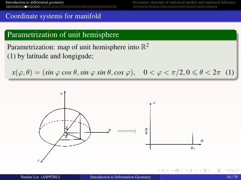
Parametrization of unit hemisphere

Parametrization: map of unit hemisphere into R2

(1) by latitude and longigude;

x(ϕ, θ) = (sin ϕ cos θ, sin ϕ sin θ, cos ϕ), 0 < ϕ < π/2, 0 6 θ < 2π (1)




Parametrization of unit hemisphere

Parametrization: map of unit hemisphere into R2

(2) by stereographic projections.

x(u, v) = (2u

1 + u2 + v2 ,2v

1 + u2 + v2 ,1− u2 − v2

1 + u2 + v2 ) where u2 + v2 6 1 (2)



Examples of Manifold: colors

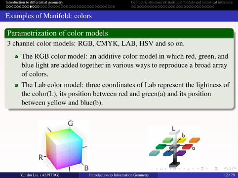
Parametrization of color models3 channel color models: RGB, CMYK, LAB, HSV and so on.

The RGB color model: an additive color model in which red, green, andblue light are added together in various ways to reproduce a broad arrayof colors.

The Lab color model: three coordinates of Lab represent the lightness ofthe color(L), its position between red and green(a) and its positionbetween yellow and blue(b).




Parametrization of color modelsParametrization: map of color into R3

Examples:



Submanifolds

SubmanifoldsDefinition: a submanifold M of a manifold S is a subset of S which itself hasthe structure of a manifoldAn open subset of n-dimensional manifold forms an n-dimensionalsubmanifold.One way to construct m(<n)dimensional manifold: fix n-m coordinates.

Examples:



Submanifolds

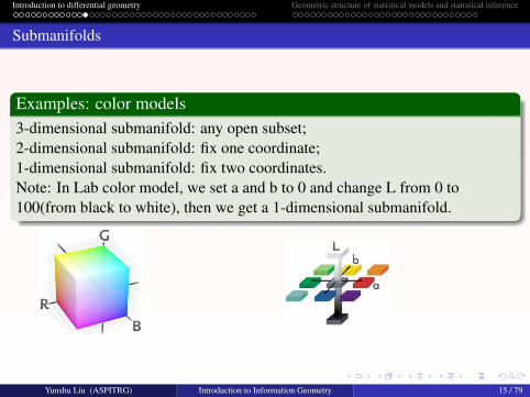
Examples: color models3-dimensional submanifold: any open subset;2-dimensional submanifold: fix one coordinate;1-dimensional submanifold: fix two coordinates.Note: In Lab color model, we set a and b to 0 and change L from 0 to100(from black to white), then we get a 1-dimensional submanifold.



Curves and Tangent vector of Curves

CurvesCurve γ: I → S from some interval I(⊂ R) to S.Examples: curve on sphere, set of probability distribution, set of linearsystems.Using coordinate system {ξi} to express the point γ(t) on the curve(where t ∈I): γi(t) = ξi(γ(t)), then we get γ(t) = [γ1(t), · · · , γn(t)].

C∞CurvesC∞: infinitely many times differentiable(sufficiently smooth).If γ(t) is C∞ for t ∈ I, we call γ a C∞ on manifold S.



Tangent vector of Curves

A tangent vector is a vector that is tangent to a curve or surface at a givenpoint.When S is an open subset of Rn, the range of γ is contained within a singlelinear space, hence we consider the standard derivative:

γ(a) = limh→0

γ(a + h)− γ(a)

h(3)

In general, however, this is not true, ex: the range of γ in a color modelThus we use a more general ”derivative” instead:

γ(a) =

n∑i=1

γi(a)(∂

∂ξi )p (4)

where γi(t) = ξi ◦ γ(t), γi(a) = ddtγ

i(t)|t=a and ( ∂∂ξi )p is an operator which

maps f → ( ∂f∂ξi )p for given function f : S→ R.



Tangent space

Tangent spaceTangent space at p: a hyperplane Tp containing all the tangents of curvespassing through the point p ∈ S. (dim Tp(S) = dim S)

Tp(S) = {n∑

i=1

ci(∂

∂ξi )p|[c1, · · · , cn] ∈ Rn}

Examples: hemisphere and color

Figure : Tangent vector and tangent space in unit hemisphere



Vector fields

Vector fieldsVector fields: a map from each point in a manifold S to a tangent vector.Consider a coordinate system {ξi} for a n-dimensional manifold, clearly∂i = ∂

∂ξi are vector fields for i = 1, · · · , n.



Riemannian Metrics

Riemannian Metrics: an inner product of two tangent vectors(D and D′ ∈

Tp(S)) which satisfy 〈 D, D′ 〉p ∈ R, and the following condition hold:

Linearity : 〈aD + bD′,D′′〉p = a〈D,D′′〉p + b〈D′ ,D′′〉p

Symmetry : 〈D,D′〉p = 〈D′ ,D〉pPositive− definiteness : If D 6= 0 then 〈D,D〉p > 0

The components {gij} of a Riemannian metric g w.r.t. the coordinate system{ξi} are defined by gij = 〈 ∂i, ∂j 〉, where ∂i = ∂

∂ξi.



Riemannian Metrics

Examples of inner product:

For X = (x1, · · · , xn) and Y = (y1, · · · , yn), we can define inner productas 〈X,Y〉1 = X · Y =

∑ni=1 xiyi, or 〈X,Y〉2 = YMX, where M is any

symmetry positive-definite matrix.

For random variables X and Y, the expected value of their product:〈X,Y〉 = E(XY)

For square real matrix, 〈A,B〉 = tr(ABT)



Riemannian Metrics

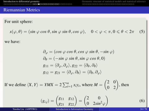
For unit sphere:

x(ϕ, θ) = (sin ϕ cos θ, sin ϕ sin θ, cos ϕ), 0 < ϕ < π, 0 6 θ < 2π (5)

we have:

∂ϕ = (cos ϕ cos θ, cos ϕ sin θ,−sin ϕ)

∂θ = (−sin ϕ sin θ, sin ϕ cos θ, 0)

g11 = 〈∂ϕ, ∂ϕ〉, g22 = 〈∂θ, ∂θ〉g12 = g21 = 〈∂ϕ, ∂θ〉 = 〈∂θ, ∂ϕ〉

If we define 〈X,Y〉 = YMX = 2∑n

i=1 xiyi, where M =

(2 00 2

), then

(gi,j) =

(g11 g12g21 g22

)=

(2 00 2sin2ϕ

)(6)



Affine connection

Parallel translation along curvesLet γ: [a, b]→ S be a curve in S, X(t) be a vector field mapping each pointγ(t) to a tangent vector, if for all t ∈ [a, b] and the corresponding infinitesimaldt, the corresponding tangent vectors are linearly related, that is to say thereexist a linear mapping Πp,p′ , such that X(t + dt) = Πp,p′ (X(t)) for t ∈ [a, b],we say X is parallel along γ, and call Πγ the parallel translation along γ.Linear mapping: additivity and scalar multiplication.

Figure : Translation of a tangent vector along a curveYunshu Liu (ASPITRG) Introduction to Information Geometry 25 / 79


Affine connection

Affine connection: relationships between tangent space at different points.Recall:

Natural basis of the coordinate system [ξi]: (∂i)p = ( ∂∂ξi )p: an operator

which maps f → ( ∂f∂ξi )p for given function f : S→ R at p.

Tangent space:

Tp(S) = {n∑

i=1

ci(∂

∂ξi )p|[c1, · · · , cn] ∈ Rn}

Tangent vector(elements in Tangent space) can be represented as linearcombinations of ∂i.

Tangent space Tp → Tangent vector Xp → Natural basis (∂i)p = ( ∂∂ξi )p



Affine connection

If the difference between the coordinates of p and p′

are very small, that wecan ignore the second-order infinitesimals (dξi)(dξj), wheredξi = ξi(p

′)− ξi(p), then we can express difference between Πp,p′ ((∂j)p) and

((∂j)p′ ) as a linear combination of {dξ1, · · · , dξn}:

Πp,p′ ((∂j)p) = (∂j)p′ −∑i,k

(dξi(Γkij)p(∂k)p′ ) (7)

where {(Γkij)p; i, j, k = 1, · · · , n} are n3 numbers which depend on the point p.

From X(t) =∑n

i=1 Xi(t)(∂i)p and X(t + dt) =∑n

i=1(Xi(t + dt)(∂i)p′ ), wehave

Πp,p′ (X(t)) =∑i,j,k

({Xk(t)− dtγi(t)Xj(t)(Γkij)p}(∂k)p′ ) (8)



Affine connection

Πp,p′ ((∂j)p) = (∂j)p′ −∑i,k

(dξi(Γkij)p(∂k)p′ )



Connection coefficients(Christoffel’s symbols): (Γkij)p

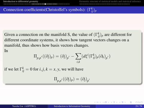
Given a connection on the manifold S, the value of (Γkij)p are different for

different coordinate systems, it shows how tangent vectors changes on amanifold, thus shows how basis vectors changes.In

Πp,p′ ((∂j)p) = (∂j)p′ −∑i,k

(dξi(Γkij)p(∂k)p′ )

if we let Γkij = 0 for i, j, k = x, y, we will have

Πp,p′ ((∂j)p) = (∂j)p′




Given a connection on a manifold S, Γki,j depend on coordinate system. Define

a connection which makes Γki,j to be zero in one coordinate system, we will

get non-zero connection coefficients in some other coordinate systems.

Example: If it is desired to let the connection coefficients for CartesianCoordinates of a 2D flat plane to be zero, Γk

ij = 0 for i, j, k = x, y, we cancalculate the connection coefficients for Polar Coordinates: Γϕrϕ = Γϕϕr = 1

r ,Γrϕϕ = −r, and Γk

ij = 0 for all others.




Example(cont.):Now if we want to let the connection coefficients for Polar Coordinates to bezero, Γk

ij = 0 for i, j, k = r, ϕ, we can calculate the connection coefficients for

Polar Coordinates: Γxxx = − sin2 ϕ cosϕ

r , Γyxx = sinϕ(1+cos2 ϕ)

r ,

Γxxy = Γx

yx = − sin3 ϕr , Γy

xy = Γyyx = − cos3 ϕ

r , Γxyy = cosϕ(1+sin2 ϕ)

r , and

Γyyy = − sinϕ cos2 ϕ

r .



Affine connection

Covariant derivative along curves

Derivative: dX(t)dt = limdt→0

X(t+dt)−X(t)dt , what if X(t) and X(t + dt) lie in

different tangent spaces? Xt(t + dt) = Πγ(t+dt),γ(t)(X(t + dt))

δX(t) = Xt(t + dt)− X(t) = Πγ(t+dt),γ(t)(X(t + dt))− X(t)



Affine connection

Covariant derivative along curves

We call δX(t)dt the covariant derivative of X(t):

δX(t)dt

= limdt→0

Xt(t + dt)− X(t)dt

=Πγ(t+dt),γ(t)(X(t + dt))− X(t)

dt(9)

Πγ(t+dt)(X(t + dt)) =∑i,j,k

({Xk(t + dt) + dtγi(t)Xj(t)(Γkij)γ(t)}(∂k)γ(t))(10)

δX(t)dt

=∑i,j,k

({Xk(t) + γi(t)Xj(t)(Γkij)γ(t)}(∂k)γ(t)) (11)



Affine connection

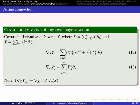
Covariant derivative of any two tangent vector

Covariant derivative of Y w.r.t. X, where X =∑n

i=1(Xi∂i) andY =

∑ni=1(Y i∂i):

∇XY =∑i,j,k

(Xi{∂iYk + Y jΓkij}∂k) (12)

∇∂i∂j =

n∑k=1

Γkij∂k (13)

Note: (∇XY)p = ∇XpY ∈ Tp(S)



Examples of Affine connection

metric connectionDefinition: If for all vector fields X,Y,Z ∈ T (S),

Z〈X,Y〉 = 〈∇ZX,Y〉+ 〈X,∇ZY〉.

where Z〈X,Y〉 denotes the derivative of the function 〈X,Y〉 along this vectorfield Z, we say that∇ is a metric connection w.r.t. g.Equivalent condition: for all basis ∂i, ∂j, ∂k ∈ T (S),

∂k〈∂i, ∂j〉 = 〈∇∂k∂i, ∂j〉+ 〈∂i,∇∂k∂i〉.

Property: parallel translation on a metric connection preserves inner products,which means parallel transport is an isometry.

〈Πγ(D1),Πγ(D2)〉q = 〈D1,D2〉p.



Examples of Affine connection

Levi-Civita connectionFor a given connection, when Γk

ij = Γkji hold for all i, j and k, we call it a

symmetric connection or torsion-free connection.From∇∂i∂j =

∑nk=1 Γk

ij∂k, we know for a symmetric connection:∇∂i∂j = ∇∂j∂i

If a connection is both metric and symmetric, we call it the Riemannianconnection or the Levi-Civita connection w.r.t. g.



Flatness

Affine coordinate system

Let {ξi} be a coordinate system for S, we call {ξi} an affine coordinate systemfor the connection∇ if the n basis vector fields ∂i = ∂

∂ξi are all parallel on S.Equivalent conditions for a coordinate system to be an affine coordinatesystem:

∇∂i∂j =∑n

k=1(Γkij∂k) = 0 for all i and j (14)

Γkij = 0 for all i, j and k (15)

FlatnessS is flat w.r.t the connection∇: an affine coordinate system exist for theconnection∇.



Flatness

Examples:

∇∂i∂j =∑n

k=1(Γkij∂k) = 0 for all i and j

Γkij = 0 for all i, j and k



Flatness

Curvature R and torsion T of a connection

R(∂i, ∂j)∂k =∑

l

(Rlijk∂l) and T(∂i, ∂j) =

∑k

(Tkij∂k) (16)

where Rlijk and Tk

ij can be computed in the following way:

Rlijk = ∂iΓ

ljk − ∂jΓ

lik + Γl

ihΓhjk − Γl

jhΓhik (17)

Tkij = Γk

ij − Γkji (18)

If a connection is flat, then T=R=0;If T= 0, Γk

ij = 0 for all i, j and k, we get the symmetry connnection.



Flatness

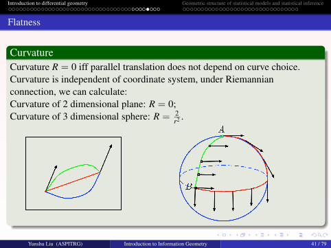
CurvatureCurvature R = 0 iff parallel translation does not depend on curve choice.Curvature is independent of coordinate system, under Riemannianconnection, we can calculate:Curvature of 2 dimensional plane: R = 0;Curvature of 3 dimensional sphere: R = 2

r2 .



Autoparallel submanifold

Equivalent condition for a submanifold M of S to be autoparallel

∇XY ∈ T (M) for ∀X,Y ∈ T (M) (19)

∇∂a∂b ∈ T (M) for all a and b (20)

∇∂a∂b =∑

c

(Γcab∂c) (21)

where ∂a = ∂∂ua and ∂b = ∂

∂ub are the basis for submanifold M w.r.t.coordinate system {ui}.

Examples of autoparallel submanifold:Open subsets of manifold S are autoparallel;A curve with the properity that all the tangent vector are parallel




GeodesicsGeodesics(autoparallel curves): A curve with tangent vector transported byparallel translation.Examples under Riemannian connection:2 dimensional flat plane: straight line3 dimensional sphere: great circle




GeodesicsThe geodesics with respect to the Riemannian connection are known tocoincide with the shortest curve joining two points.Shortest curve: curve with the shortest length.Length of a curve γ : [a, b]→ S:

‖γ‖ =

∫ b

a‖dγ

dt‖dt =

∫ b

a

√gijγiγjdt (22)



Part II

Geometric structure of statistical models and statisticalinference



Motivation

MotivationConsider the set of probability distributions as a manifold.

Analysis the relationship between the geometric structure of the manifold andstatistical estimation.

Introduce concepts like metric, affine connection on statistical models andstudying quantities such as distance, the tangent space (which provides linearapproximations), geodesics and the curvature of a manifold.



Statistical models

Statistical models

P(X ) = {p : X → R | p(x) > 0 (∀x ∈ X ),

∫p(x)dx = 1} (23)

Example Normal Distribution:

X = R, n = 2, ξ = [µ, σ],Ξ = {[µ, σ]| −∞ < µ <∞, 0 < σ <∞}

p(x, ξ) =1√2πσ

exp−(x− µ)2

2σ2



Geometric structure of statistical models and statistical inference

Basic conceptsThe Fisher metric and α-connectionExponential familyDivergence and Geometric statistical inference



The Fisher information matrix

Fisher information matrix G(ξ) = [gi,j(ξ)], and

gi,j(ξ) = Eξ[∂i`ξ∂j`ξ] =

∫∂i`(x; ξ)∂j`(x; ξ)p(x; ξ)dx

where `ξ = `(x; ξ) = log p(x; ξ) and Eξ denotes the expectation w.r.t. thedistribution pξ.

Motivation:Sufficient statistic and Cramer-Rao bound



The Fisher information matrix

Sufficient statisticSufficient statistic: for Y = F(X), given the distribution p(x; ξ) of X, we havep(x; ξ) = q(F(x); ξ)r(x; ξ), if r(x; ξ) does not depend on ξ for all x, we saythat F is a sufficient statistic for the model S. Then we can writep(x; ξ) = q(y; ξ)r(x).A sufficient statistic is a function whose value contains all the informationneeded to compute any estimate of the parameter (e.g. a maximum likelihoodestimate).

Fisher information matrix and sufficient statisticLet G(ξ) be the Fisher information matrix of S = p(x; ξ), and GF(ξ) be theFisher information matrix of the induced model SF = q(y; ξ), then we haveGF(ξ) 6 G(ξ) in the sense that ∆G(ξ) = GF(ξ)− G(ξ) is positivesemidefinite. ∆G(ξ) = 0 iff. F is a sufficient statistic for S.



Cramer-Rao inequality

Cramer-Rao inequalityThe variance of any unbiased estimator is at least as high as the inverse of theFisher information.Unbiased estimator ξ: Eξ[ξ(X)] = ξ

The variance-covariance matrix Vξ[ξ] = [vijξ ] where

vijξ = Eξ[(ξi(X)− ξi)(ξj(X)− ξj)]

Thus Cramer-Rao inequality state that Vξ[ξ] > G(ξ)−1, and an unbiasedestimator ξ satisfying Vξ[ξ] = G(ξ)−1 is called an efficient estimator.



α-connection

α-connection

Let S = {pξ} be an n-dimensional model, and consider the function Γ(α)ij,k

which maps each point ξ to the following value:

(Γ(α)ij,k )ξ = Eξ[(∂i∂j`ξ +

1− α2

∂i`ξ∂j`ξ)(∂k`ξ)] (24)

where α is an arbitrary real number. We defined an affine connection∇(α)

which satisfy: ⟨∇(α)∂i∂j, ∂k

⟩= Γ

(α)ij,k (25)

where g = 〈, 〉 is the Fisher metric. We call∇(α) the α-connection



α-connection

Properties of α-connectionα-connection is a symmetric connection

Relationship between α-connection and β-connection:

Γ(β)ij,k = Γ

(α)ij,k +

α− β2

E[∂i`ξ∂j`ξ∂k`ξ]

The 0-connection is the Riemannian connection with respect to theFisher metric.

Γ(β)ij,k = Γ

(0)ij,k +

−β2

E[∂i`ξ∂j`ξ∂k`ξ]

∇(α) =1 + α

2∇(1) +

1− α2∇(−1)



Exponential family

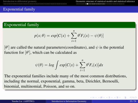
Exponential family

p(x; θ) = exp[C(x) +

n∑i=1

θiFi(x)− ψ(θ)]

[θi] are called the natural parameters(coordinates), and ψ is the potentialfunction for [θi], which can be calculated as

ψ(θ) = log∫

exp[C(x) +

n∑i=1

θiFi(x)]dx

The exponential families include many of the most common distributions,including the normal, exponential, gamma, beta, Dirichlet, Bernoulli,binomial, multinomial, Poisson, and so on.



Exponential family

Exponential familyExamples: Normal Distribution

p(x;µ, σ) =1√2πσ

e−(x−µ)2

2σ2 (26)

where C(x) = 0,F1(x) = x,F2(x) = x2, and θ1 = µσ2 , θ

2 = − 12σ2 are the

natural parameters, the potential function is :

ψ = −(θ1)2

4θ2 +12

log(− πθ2 ) =

µ2

2σ2 + log(√

2πσ) (27)



Mixture family

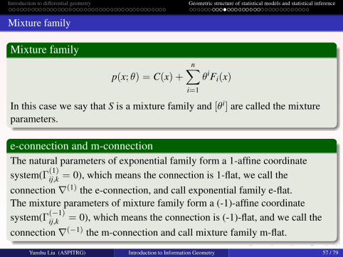
Mixture family

p(x; θ) = C(x) +

n∑i=1

θiFi(x)

In this case we say that S is a mixture family and [θi] are called the mixtureparameters.

e-connection and m-connectionThe natural parameters of exponential family form a 1-affine coordinatesystem(Γ(1)

ij,k = 0), which means the connection is 1-flat, we call theconnection∇(1) the e-connection, and call exponential family e-flat.The mixture parameters of mixture family form a (-1)-affine coordinatesystem(Γ(−1)

ij,k = 0), which means the connection is (-1)-flat, and we call theconnection∇(−1) the m-connection and call mixture family m-flat.



Dual connection

Dual connectionDefinition: Let S be a manifold on which there is given a Riemannian metricg and two affine connection∇ and ∇∗. If for all vector fields X,Y,Z ∈ T (S),

Z < X,Y >=< ∇ZX,Y > + < X,∇∗ZY > (28)

hold, we say that∇ and∇∗ are duals of each other w.r.t. g and call one thedual connection of the other.Additional, we call the triple (g,∇, ∇∗) a dualistic structure on S.



Dual connection

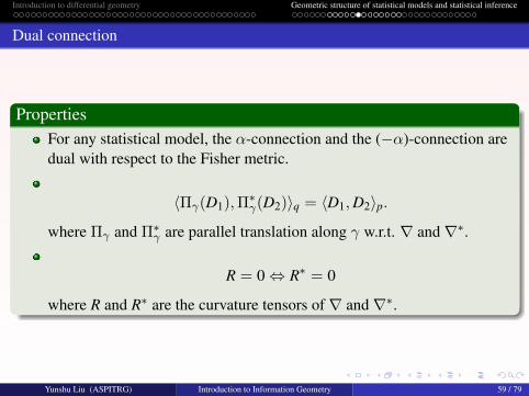
PropertiesFor any statistical model, the α-connection and the (−α)-connection aredual with respect to the Fisher metric.

〈Πγ(D1),Π∗γ(D2)〉q = 〈D1,D2〉p.

where Πγ and Π∗γ are parallel translation along γ w.r.t. ∇ and ∇∗.

R = 0⇔ R∗ = 0

where R and R∗ are the curvature tensors of∇ and ∇∗.



Dually flat spaces and dual coordinate system

Dually flat spacesLet (g,∇,∇∗) be a dualistic structure on a manifold S, then we haveR = 0⇔ R∗ = 0, and if the connnection∇ and ∇∗ are bothsymmetric(T = T∗ = 0), then we see that∇-flatness and∇∗-flatness areequivalent.We call (S, g,∇,∇∗) a dually flat space if both duals∇ and∇∗ are flat.Examples: Since α-connections and −α-connections are dual w.r.t. Fishermetric and α-connections are symmetry, we have for any statistical model Sand for any real number α

S is α− flat⇔ S is (−α)− flat (29)



Dually flat spaces and dual coordinate system

Dual coordinate system

For a particular∇-affine coordinate system [θi], if we choose a corresponding∇∗-affine coordinate system [ηj] such that

g = 〈∂i, ∂j〉 = δj

i

where ∂i = ∂∂θi and ∂j = ∂

∂ηj.

Then we say the two coordinate systems mutually dual w.r.t. metric g, andcall one the dual coordinate system of the other.

Existence of dual coordinate systemA pair of dual coordinate system exist if and only if (S, g,∇,∇∗) is a duallyflat space.



Legendre transformations

Consider mutually dual coordinate system [θi] and [ηi] with functionsψ : S→ R and ϕ : S→ R satisfy the following equations:

∂iψ = ηi

∂iϕ = θi

gi,j = ∂iηj = ∂jηi = ∂i∂jψ

ϕ(η) = maxθ{θiηi − ψ(θ)}ψ(θ) = maxη{θiηi − ϕ(η)}



Legendre transformations

Geometric interpretation forf ∗(p) = maxx(px− f (x)):A convex function f (x) is shown in red, andthe tangent line at point (x0, f (x0)) is shownin blue. The tangent line intersects thevertical axis at (0,−f ∗) and f ∗ is the value ofthe Legendre transform f ∗(p0), wherep0 = f (x0). Note that for any other point onthe red curve, a line drawn through that pointwith the same slope as the blue line will havea y-intercept above the point (0,−f ∗),showing that is indeed a maximum.



Examples of Legendre transformations

Examples:

The Legendre transform of f (x) = 1p |x|

p (where 1 < p <∞) isf ∗(x∗) = 1

q |x∗|q (where 1 < q <∞),

The Legendre transform of f (x) = ex is f ∗(x∗) = x∗ln x∗ − x∗ (wherex∗ > 0),

The Legendre transform of f (x) = 12 xTAx is f ∗(x∗) = 1

2 x∗TA−1x∗,

The Legendre transform of f (x) = |x| is f ∗(x∗) = 0 if x∗ 6 1, andf ∗(x∗) =∞ if x∗ > 1.



The natural parameter and dual parameter of Exponential family

For distribution p(x; θ) = exp[C(x) +∑n

i=1 θiFi(x)− ψ(θ)], [θi] are

called the natural parameters

If we define ηi = Eθ[Fi] =∫

Fi(x)p(x; θ)dx, we can verify [ηi] is a(-1)-affine coordinate system dual to [θi], we call this [ηi] the expectationparameters or the dual parameters.



The natural parameter and dual parameter of Exponential family

Recall: Normal Distribution

p(x;µ, σ) =1√2πσ

e−(x−µ)2

2σ2 (30)

where C(x) = 0,F1(x) = x,F2(x) = x2, and θ1 = µσ2 , θ

2 = − 12σ2 are the

natural parameters, the potential function is :

ψ = −(θ1)2

4θ2 +12

log(− πθ2 ) =

µ2

2σ2 + log(√

2πσ) (31)

The dual parameter are calculated as η1 = ∂ψ∂θ1 = µ = − θ1

2θ2 ,

η2 = ∂ψ∂θ2 = µ2 + σ2 = (θ1)2−2θ2

4(θ2)2 , It has potential function:

ϕ = −12

(1 + log(− πθ2 )) = −1

2(1 + log(2π)) + 2logσ) (32)



Divergences

Let S be a manifold and suppose that we are given a smooth functionD = D(·‖·) : S× S→ R satisfying for any p, q ∈ S:

D(p‖q) > 0 with equality iff . p = q) (33)

Then we introduce a distance-like measure of the separation between twopoints.



Divergence, semimetrics and metrics

A distance satisfying positive-definiteness, symmetry and triangleinequality is called a metric;

A distance satisfying positive-definiteness and symmetry is calledsemimetrics;

A distance satisfying only positive-definiteness is called a divergence.



Kullback-Leibler divergence

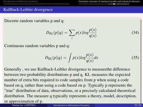
Discrete random variables p and q:

DKL(p‖q) =∑

i

p(x)logp(x)

q(x)(34)

Continuous random variables p and q:

DKL(p‖q) =

∫p(x)log

p(x)

q(x)dx (35)

Generally , we use Kullback-Leibler divergence to measurethe differencebetween two probability distributions p and q. KL measures the expectednumber of extra bits required to code samples from p when using a codebased on q, rather than using a code based on p. Typically p represents the”true” distribution of data, observations, or a precisely calculated theoreticaldistribution. The measure q typically represents a theory, model, description,or approximation of p.



Bregman divergence

Bregman divergence associatedwith F for points p, q ∈ ∆ is :BF(x‖y) =F(y)−F(x)− 〈(y− x),∇F(x)〉,where F(x) is a convex functiondefined on a closed convex set∆.

Examples:F(x) = ‖x‖2, then BF(x‖y) = ‖x− y‖2.More generally, if F(x) = 1

2 xTAx, then BF(x‖y) = 12(x− y)TA(x− y).

KL divergence:if F =∑

i x logx−∑

x, we get KullbackLeibler divergence.



Canonical divergence

Canonical divergence(a divergence for dually flat space)

Let (S, g,∇,∇∗) be a dually flat space, and {[θi], [ηj]} be mutually dual affinecoordinate systems with potentials {ψ,ϕ}, then the canonicaldivergence((g,∇)− divergence) is defined as:

D(p‖q) = ψ(p) + ϕ(q)− θi(p)ηj(q) (36)




Properties:Relation between (g,∇)− divergence and (g,∇∗)− divergence:D∗(p‖q) = D(q‖p)

If M is a autoparallel submanifold w.r.t. either∇ or ∇∗, then the(gM,∇M)-divergence DM = D|M×M is given by DM(p‖q) = D(p‖q)

If ∇ is a Riemannian connection(∇ = ∇∗) which is flat on S, there exista coordinate system which is self-dual(θi = ηi), thenϕ = ψ = 1

2∑

i(θi)2, then the canonical divergence is

D(p‖q) =12{d(p, q)}2

where d(p, q) =√∑

i{θi(p)− θi(q)}2




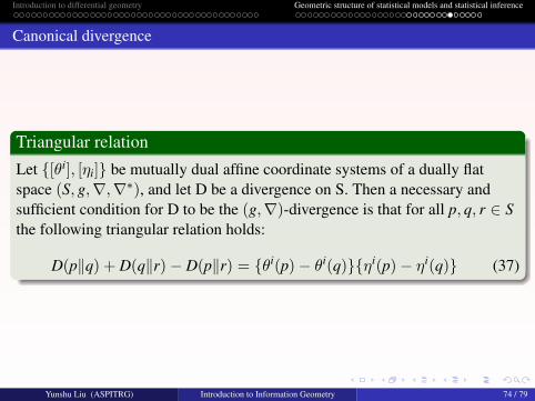
Triangular relation

Let {[θi], [ηi]} be mutually dual affine coordinate systems of a dually flatspace (S, g,∇,∇∗), and let D be a divergence on S. Then a necessary andsufficient condition for D to be the (g,∇)-divergence is that for all p, q, r ∈ Sthe following triangular relation holds:

D(p‖q) + D(q‖r)− D(p‖r) = {θi(p)− θi(q)}{ηi(p)− ηi(q)} (37)




Pythagorean relationLet p, q, and r be three points in S. Let γ1 be the∇-geodesic connecting p andq, and let γ2 be the∇∗-geodesic connecting q and r. If at the intersection q thecurve γ1 and γ2 are orthogonal(with respect to the inner product g), then wehave the following Pythagorean relation.

D(p‖r) = D(p‖q) + D(q‖r) (38)

Figure :Yunshu Liu (ASPITRG) Introduction to Information Geometry 75 / 79



Projection theoremLet p be a point in S and let M be a submanifold of S which is∇∗-autoparallel. Then a necessary and sufficient condition for a point q in Mto satisfy

D(p‖q) = minr∈MD(p‖r) (39)

is for the∇-geodesic connecting p and q to be orthogonal to M at q.

Figure :Yunshu Liu (ASPITRG) Introduction to Information Geometry 76 / 79



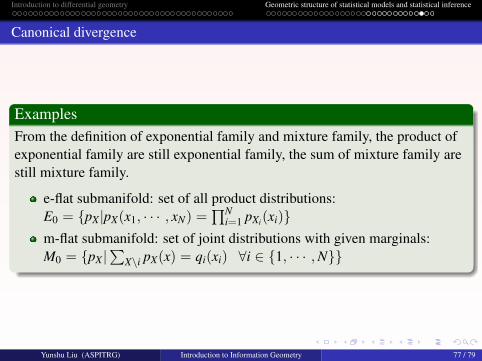
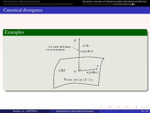
ExamplesFrom the definition of exponential family and mixture family, the product ofexponential family are still exponential family, the sum of mixture family arestill mixture family.

e-flat submanifold: set of all product distributions:E0 = {pX|pX(x1, · · · , xN) =

∏Ni=1 pXi(xi)}

m-flat submanifold: set of joint distributions with given marginals:M0 = {pX|

∑X\i pX(x) = qi(xi) ∀i ∈ {1, · · · ,N}}




Examples



Thanks!

Thanks!Question?


introduction to information geometryintroduction to differential geometry geometric structure of...

Documents