Introduction to Information Retrieval(Manning, Raghavan, Schutze)

Chapter 6Scoring term weighting and the

vector space model

Ranked retrievaln Thus far, our queries have all been Boolean.

n Documents either match or don’tn Good for expert users with precise understanding of

their needs and the collection.n Also good for applications, which can easily consume

1000s of resultsn Not good for the majority of users.

n Most users incapable of writing Boolean queries (or they are, but they think it’s too much work).

n Most users don’t want to wade through 1000s of results.n This is particularly true of web search.

Problem with Boolean search: feast or famine

n Boolean queries often result in either too few (=0) or too many (1000s) results.

n Query 1: “standard user dlink 650”n 200,000 hits

n Query 2: “standard user dlink 650 no card found”n 0 hits

n It takes skill to come up with a query that produces a manageable number of hits.n AND gives too few; OR gives too many

Ranked retrieval modelsn Rather than a set of documents satisfying a

query expression, in ranked retrieval, the system returns an ordering over the (top) documents in the collection for a query

n Free text queries: rather than a query language of operators and expressions, the user’s query is just one or more words in natural languagen Ranked retrieval has normally been associated

with free text queries and vice versan With a ranked list of documents it does not

matter how large the retrieved set is. n Just show top k results, don’t overwhelm the user

Scoring as the basis of ranked retrieval

n We wish to return in order the documents most likely to be useful to the searcher

n How can we rank-order the documents in the collection with respect to a query?

n Assign a score – say in [0, 1] – to each documentn This score measures how well document and

query “match”.

Query-document matching scores

n We need a way of assigning a score to a query/document pair

n Let’s start with a one-term queryn If the query term does not occur in the document:

score should be 0n The more frequent the query term in the

document, the higher the score (should be)n We will look at a number of alternatives for this.

Take 1: Jaccard coefficient

n A commonly used measure of overlap of two sets A and B

n jaccard(A,B) = |A ∩ B| / |A ∪ B|n jaccard(A,A) = 1n jaccard(A,B) = 0 if A ∩ B = 0

n Always assigns a number between 0 and 1.

Jaccard coefficient: Scoring example

n What is the query-document match score that the Jaccard coefficient computes for each of the two documents below?

n Query: ides of marchn Document 1: caesar died in marchn Document 2: the long march

Issues with Jaccard for scoring

n It doesn’t consider term frequency (how many times a term occurs in a document)n tf weight

n Rare terms in a collection are more informative than frequent terms. Jaccard doesn’t consider this informationn idf weight

n We need a more sophisticated way of normalizing for lengthn cosine

Bag of words model

n Vector representation doesn’t consider the ordering of words in a document

n John is quicker than Mary and Mary is quicker than John have the same vectors

n This is called the bag of words model.

Term frequency

n The term frequency tft,d of term t in document d is defined as the number of times that t occurs in d.

n We want to use term frequency when computing query-document match scores. But how?

n Rawtermfrequencymaynotbewhatwewant:n Adocumentwith10occurrencesofthetermismorerelevantthanadocumentwith1occurrenceoftheterm.

n Butnot10timesmorerelevant.n Relevancedoesnotincreaseproportionallywithtermfrequency

term frequency (tf) weightn many variants for tf weight, where log-frequency

weighting is a common one, dampening the effect of raw tf (raw count)

log tft,d =

n 0 → 0, 1 → 1, 2 → 1.3, 10 → 2, 1000 → 4, etc.n The score is 0 if none of the query terms is

present in the document.

1 + log10 tft,d, if tft,d > 00, otherwise

!"#

$#

Document frequency

n Rare terms are more informative than frequent termsn Recall stop words

n Consider a term in the query that is rare in the collection (e.g., arachnocentric)

n A document containing this term is very likely to be relevant to the query arachnocentric

n → We want a high weight for rare terms like arachnocentric.

Document frequency, continued

n Consider a query term that is frequent in the collection (e.g., high, increase, line)

n A document containing such a term is more likely to be relevant than a document that doesn’t, but it’s not a sure indicator of relevance.

n For frequent terms, we want positive weights for words like high, increase, and line, but lower weights than for rare terms.

n We will use document frequency (df) to capture this in the score.

n df (≤ N) is the number of documents that contain the term

Inverse document frequency (idf) weight

n dft is the document frequency of t: the number of documents that contain tn dft is an inverse measure of the informativeness of tn Inverse document frequency is a direct measure of the

informativeness of tn We define the idf (inverse document frequency) of t by

n use log to dampen the effect of N/dftn Most common variant of idf weight

tt N/df log idf 10=

idf example, suppose N= 1 millionterm dft idftcalpurnia 1 6

animal 100 4

sunday 1,000 3

fly 10,000 2

under 100,000 1

the 1,000,000 0

There is one idf value for each term t in a collection.

)/df( log idf 10 tt N=

Effect of idf on rankingn Doesidfhaveaneffectonrankingforone-term

queries,liken iPhone

n idfhasnoeffectonrankingonetermqueriesn idfaffectstherankingofdocumentsforquerieswithatleasttwoterms

n Forthequerycapriciousperson,idfweightingmakesoccurrencesofcapricious countformuchmoreinthefinaldocumentrankingthanoccurrencesofperson.

Collection vs. Document frequencyn The collection frequency of t is the number of

occurrences of t in the collection, counting multiple occurrences.

n Example: which word is a better search term (and should get a higher weight)?

n The example suggests that df is better for weighting than cf

Word Collection frequency Document frequency

insurance 10440 3997

try 10422 8760

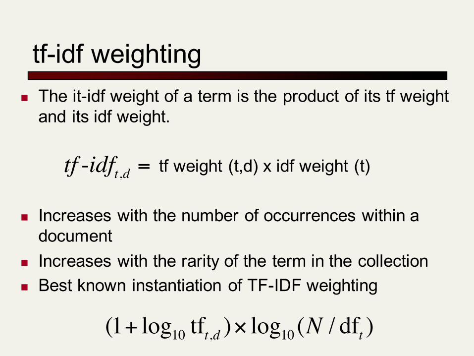
tf-idf weightingn The it-idf weight of a term is the product of its tf weight

and its idf weight.

tf weight (t,d) x idf weight (t)

n Increases with the number of occurrences within a document

n Increases with the rarity of the term in the collectionn Best known instantiation of TF-IDF weighting

tf -idft,d =

(1+ log10 tft,d )× log10 (N / dft )

Note on terminology

n terminology is not standardized in the textbook/literature. tft,d sometimes refers to the raw count, sometimes the weight derived from the raw count.

n We use tft,d to mean the raw count only. So tf (raw count) and tf weight (weight derived from the raw count) are different. tf can be used as tf weight, but log tf is a more common variant.

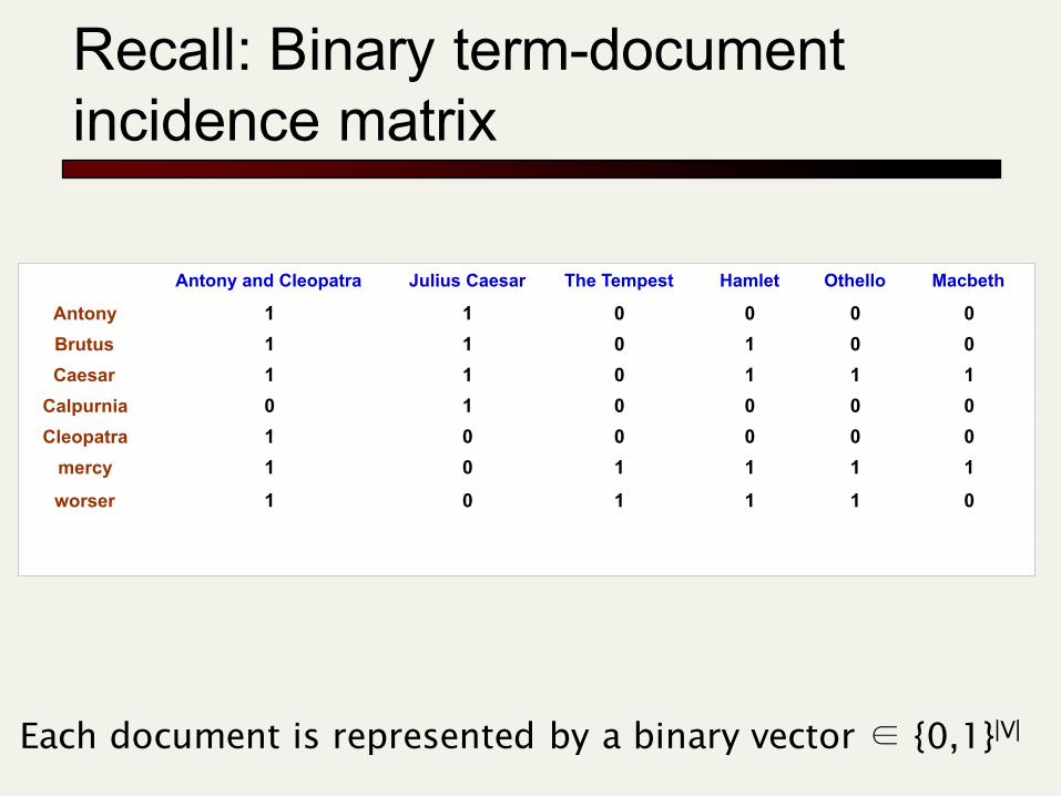
Recall: Binary term-document incidence matrix

Antony and Cleopatra Julius Caesar The Tempest Hamlet Othello Macbeth

Antony 1 1 0 0 0 0Brutus 1 1 0 1 0 0Caesar 1 1 0 1 1 1

Calpurnia 0 1 0 0 0 0Cleopatra 1 0 0 0 0 0

mercy 1 0 1 1 1 1worser 1 0 1 1 1 0

Each document is represented by a binary vector ∈ {0,1}|V|

Term-document count matrices

n Consider the number of occurrences of a term in a document: n Each document is a count vector in ℕv: a column below

Antony and Cleopatra Julius Caesar The Tempest Hamlet Othello Macbeth

Antony 157 73 0 0 0 0Brutus 4 157 0 1 0 0Caesar 232 227 0 2 1 1

Calpurnia 0 10 0 0 0 0Cleopatra 57 0 0 0 0 0

mercy 2 0 3 5 5 1worser 2 0 1 1 1 0

Binary → count → weight matrix

Antony and Cleopatra Julius Caesar The Tempest Hamlet Othello Macbeth

Antony 5.25 2.44 0 0 0 0Brutus 0.16 6.10 0 0.04 0 0Caesar 8.59 8.40 0 0.07 0.04 0.04

Calpurnia 0 1.54 0 0 0 0Cleopatra 2.85 0 0 0 0 0

mercy 1.51 0 2.27 3.78 3.78 0.76worser 1.37 0 0.69 0.69 0.69 0

Each document is now represented by a real-valued vector of TF-IDF weights ∈ R|V|

Documents as vectors

n So we have a |V|-dimensional vector spacen Terms are axes of the spacen Documents are points or vectors in this spacen Very high-dimensional

n hundreds of millions of dimensions when you apply this to a web search engine

n This is a very sparse vectorn most entries are zero

Example: raw counts as weights

Queries as vectors

n Key idea 1: Do the same for queries: represent them as vectors in the space

n Key idea 2: Rank documents according to their proximity to the query in this space

n proximity = similarity of vectorsn proximity ≈ inverse of distancen Recall: We do this because we want to get away

from the either-in-or-out Boolean model.n Instead: rank more relevant documents higher

than less relevant documents

Formalizing vector space proximity

n Distance between two vectorsn between two end points of the two vectorsn Euclidean distance? n a bad idea. It’s large for vectors of different lengths.

Why Euclidean distance is badThe Euclidean distance between qand d2 is large even though thedistribution of terms in the query q and the distribution ofterms in the document d2 arevery similar.

Use angle instead of distance

n Thought experiment: take a document d and append it to itself. Call this document d′.

n “Semantically” d and d′ have the same contentn The Euclidean distance between the two

documents can be quite largen The angle between the two documents is 0,

corresponding to maximal similarity.

From angles to cosines

n The following two notions are equivalent.n Rank documents in decreasing order of the angle between query

and documentn Rank documents in increasing order

of cosine(query, document)n Cosine is a monotonically decreasing

function for the interval [0o, 180o]n In general, cosine similarity ranges [-1, 1]n In the case of information retrieval, the cosine similarity of two

documents will range from 0 to 1n term frequencies (tf-idf weights) cannot be negativen The angle between two term frequency vectors cannot be greater than 90°n cosine (90) = 0, (completely unrelated) n cosine (0) = 1, (completely related)

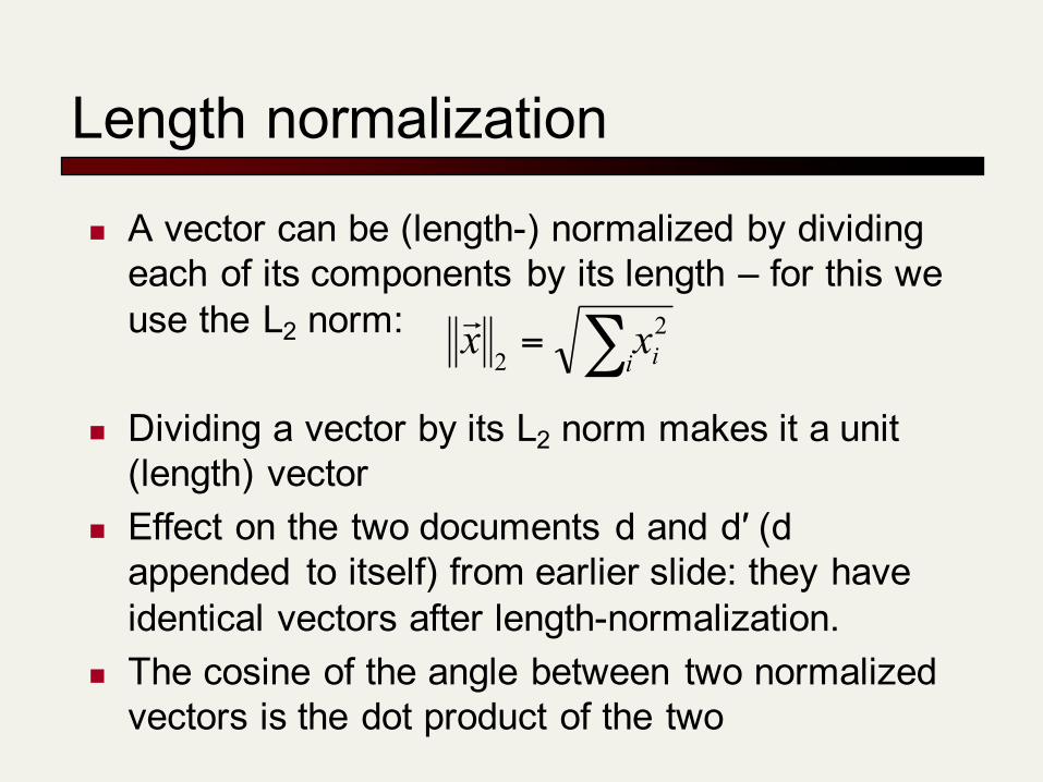
Length normalization

n A vector can be (length-) normalized by dividing each of its components by its length – for this we use the L2 norm:

n Dividing a vector by its L2 norm makes it a unit (length) vector

n Effect on the two documents d and d′ (d appended to itself) from earlier slide: they have identical vectors after length-normalization.

n The cosine of the angle between two normalized vectors is the dot product of the two

∑=i ixx 2

2

!

cosine(query,document)

cos(!q,!d ) =

!q •!d!q!d=!q!q•

!d!d=

qtdtt=1

V∑qt2

t=1

V∑ dt

2

t=1

V∑

Dot product Unit vectors

qt is the tf-idf weight of term t in the querydt is the tf-idf weight of term t in the document

cos(q,d) is the cosine similarity of q and d … or,equivalently, the cosine of the angle between q and d.

• The cosine similarity can be seen as a method of normalizing document length during comparison

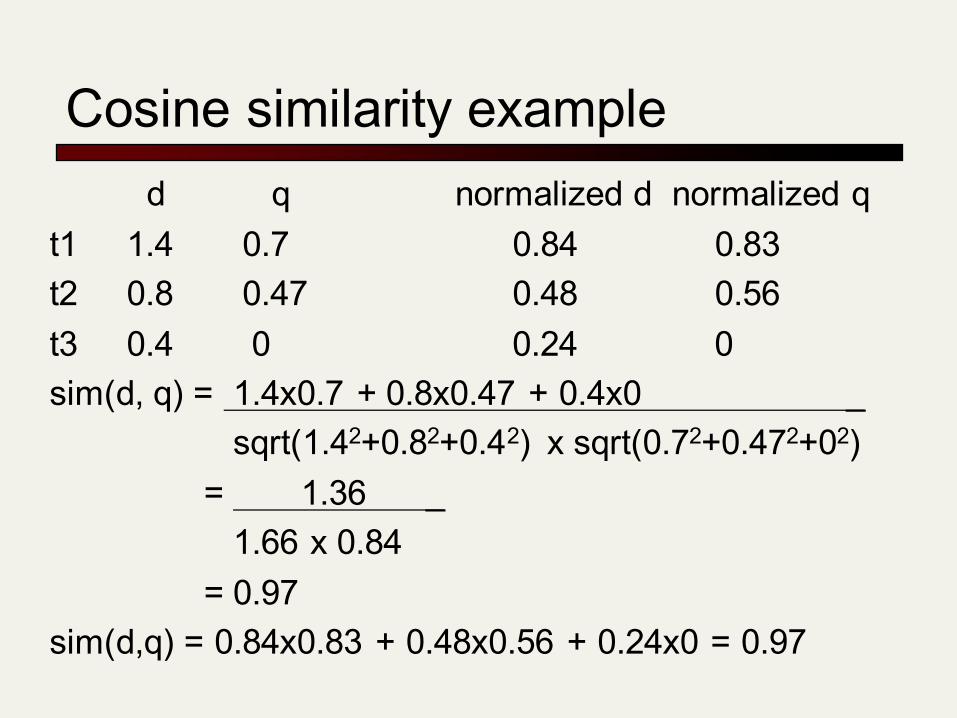
Cosine similarity exampled q normalized d normalized q

t1 1.4 0.7 0.84 0.83t2 0.8 0.47 0.48 0.56t3 0.4 0 0.24 0 sim(d, q) = 1.4x0.7 + 0.8x0.47 + 0.4x0 _

sqrt(1.42+0.82+0.42) x sqrt(0.72+0.472+02)= 1.36 _

1.66 x 0.84 = 0.97

sim(d,q) = 0.84x0.83 + 0.48x0.56 + 0.24x0 = 0.97

More on the cosine formula

cos(!q,!d ) =

!q •!d!q!d=!q!q•

!d!d=

qtdtt=1

V∑qt2

t=1

V∑ dt

2

t=1

V∑

=qtdtt∈T∑

|| q || * || d ||

• T is the set of terms q and d share in common. If T is empty, then cosine similarity = 0

• qt is the tf-idf weight of term t in the query q, i.e, tf weight(t,q) x idf weight(t)

• dt is the tf-idf weight of term t in the document d, i.e,tf weight(t,d) x idf weight(t)

• In actual implementation, do we need to represent q and d as vectors of size |V| ?

More variants of TF-IDF weighting

SMART notation: columns headed ‘n’ are acronymsfor weight schemes.

Weighting may differ in queries vs documents

n Many search engines allow for different weightings for queries vs documents

n SMART notation: denotes the combination in use in an engine, with the notation ddd.qqq, using acronyms from the previous table

n A very standard weighting scheme: lnc.ltcn Document: logarithmic tf, no idf, cosine normalization

n no idf: for both effectiveness and efficiency reasonsn Query: logarithmic tf, idf, cosine normalization

lnc.ltc examplen Query: “good news”n Document: “good news bad news”n In the table, log tf is the tf weight based on log-frequency weighting,

q is the query vector, q’ is the length-normalized q, d is the document vector, and d’ is the length-normalized d. Assume N=10,000,000

n Assume N = 10,000,000.

n The cosine similarity between q and d is the dot product of q’ and d’, which is: 0x0.52 + 0.45x0.52 + 0.89x0.68 = 0.84

n in implementation: representing vectors and computing cosine

Summary – vector space ranking

n Represent the query as a weighted TF-IDF vectorn Represent each document as a weighted TF-IDF

vectorn Compute the cosine similarity score for the query

vector and each document vectorn Rank documents with respect to the query by scoren Return the top k (e.g., k = 10) to the user

Gerard Salton

n 1927-1995. Born in Germany, Professor at Cornell (co-founded the CS department), Ph.D from Harvard in Applied Mathematics

n Father of information retrievaln Vector space modeln SMART information retrieval

systemn First recipient of SIGIR outstanding

contribution award, now called the Gerard Salton Award