MATH 499Fall 2015LaTeX basics

Note: This document was taken, almost verbatim, from Dr. Jessica Sklar, who kindly gave me permission to share it with you. The document was written a few years ago, so it is possible that some things can now be done more efficiently. I still use the LaTeX commands that I used years ago, so if you learn new tricks, please share them with me.

Document Basics(If you are using Sage, this part is already taken care of for you, but if you download some version of LaTeX onto your computer, then it’s good to know.)

Your file should be saved as a file ending with .tex.

The first line of your .tex file should be \documentclass{document_class}, typically \documentclass{article}. Other document classes include book and report.

Following \documentclass is usually a series of package inclusion commands, macro definitions, document specifications, etc. This section of your document is called your document’s “preamble.”

After the preamble, we begin your document content itself using the command \begin{document}. At the very end of your .tex file, put the command \end{document}. Your document’s contents go in between these two commands.

Throughout your file, you can add comments that will not be compiled by LaTeX by putting a % symbol at the beginning of the comment lines.

Text Mode Basics

There are two modes in LaTeX: test mode and math mode. By default when you start writing in your document, you are in text mode.

Note: You can write integers in text mode. Most other mathematical symbols need to be written in math mode. (Integers can of course also be written in math mode.)

If you press return twice in text mode, you get a new paragraph. LaTeX indents each new paragraph. If you don’t want your paragraph to be indented, type \noindent.

You can skip vertical space by typing \bigskip, \medskip, or \smallskip. You can alternatively specify exactly the amount of vertical or horizontal space that you want to skip using the commands \vspace, \vspace*, \hspace, and \hspace*; we later discuss these commands.

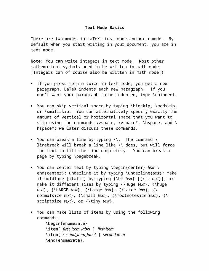
You can break a line by typing \\. The command \linebreak will break a line like \\ does, but will force the text to fill the line completely. You can break a page by typing \pagebreak.

You can center text by typing \begin{center} text \end{center}; underline it by typing \underline{text}; make it boldface [italic] by typing {\bf text} [{\it text}]; or make it different sizes by typing {\Huge text}, {\huge text}, {\LARGE text}, {\Large text}, {\large text}, {\normalsize text}, {\small text}, {\footnotesize text}, {\scriptsize text}, or {\tiny text}.

You can make lists of items by using the following commands: \begin{enumerate} \item[ first_item_label ] first item \item[ second_item_label ] second item \end{enumerate}.

An item label can be a bullet ($\bullet$), a number, a letter, etc.

If you want a bulleted list, you can just replace enumerate with itemize in the commands above.

To create some special characters, like $, %, {}, & and #, you must precede them with backslashes. (These characters are used to indicate commands within the LaTeX language, so you need to tell LaTeX you’re not giving it a command.)

To create a backslash (that is, \), type \backslash in math mode (see next section for details on math mode).

To make left quotation marks, type \lq \lq. You can also do this: `` (two tick marks), but you cannot just enter quotation marks.

To insert an extra space between characters (for instance, when two consecutive characters are too printed close together for your liking), type \, (that is, a backslash followed by a comma) for a small extra space, and type \ for a larger one. This also works in math mode. Note: if you type \ for a larger space, you will need to put a space between the \ and the next symbol in your code.

To make the word “LaTeX” appear in its trademark style, type \LaTeX.

Math Mode Basics

You put work in math mode by surrounding it by $s or $$s.

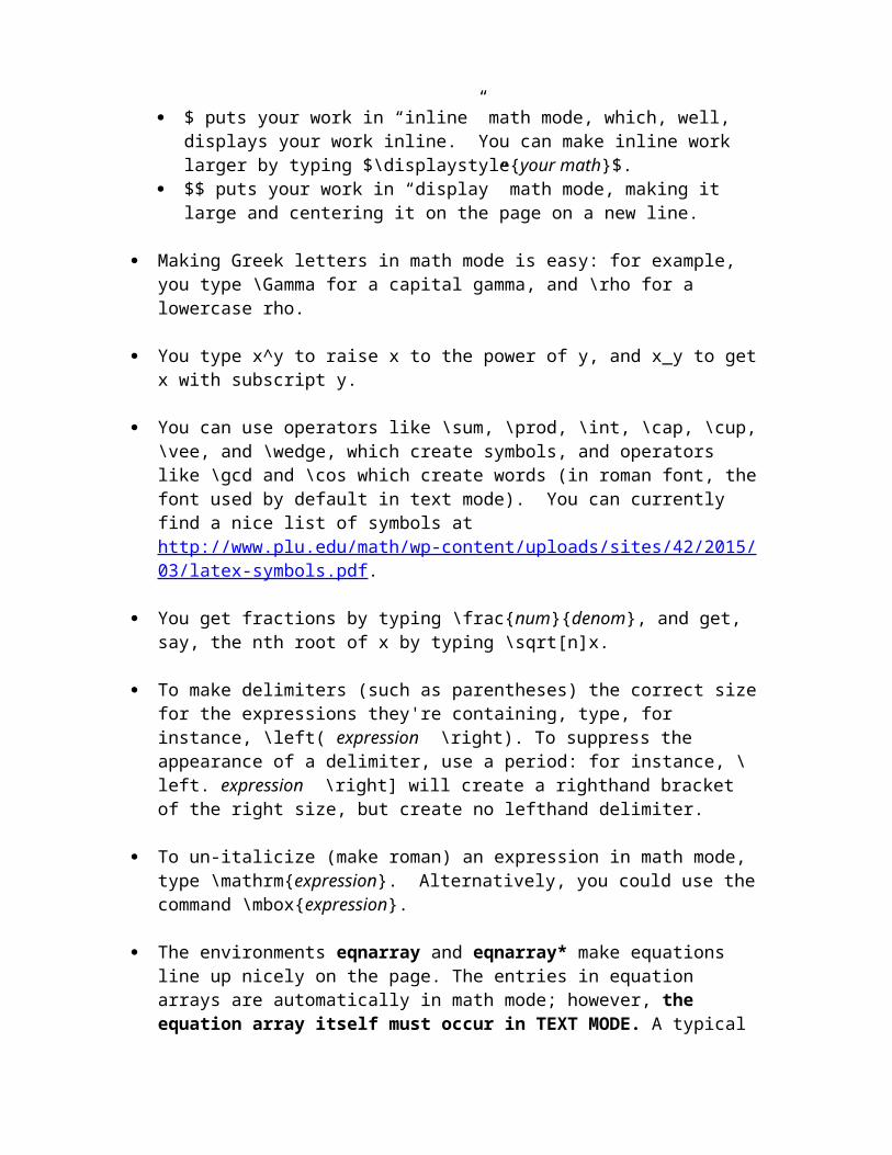
$ puts your work in “inline” math mode, which, well, displays your work inline. You can make inline work larger by typing $\displaystyle{your math}$.

$$ puts your work in “display” math mode, making it large and centering it on the page on a new line.

Making Greek letters in math mode is easy: for example, you type \Gamma for a capital gamma, and \rho for a lowercase rho.

You type x^y to raise x to the power of y, and x_y to get x with subscript y.

You can use operators like \sum, \prod, \int, \cap, \cup, \vee, and \wedge, which create symbols, and operators like \gcd and \cos which create words (in roman font, the font used by default in text mode). You can currently find a nice list of symbols at http://www.plu.edu/math/wp-content/uploads/sites/42/2015/03/latex-symbols.pdf.

You get fractions by typing \frac{num}{denom}, and get, say, the nth root of x by typing \sqrt[n]x.

To make delimiters (such as parentheses) the correct size for the expressions they're containing, type, for instance, \left( expression \right). To suppress the appearance of a delimiter, use a period: for instance, \left. expression \right] will create a righthand bracket of the right size, but create no lefthand delimiter.

To un-italicize (make roman) an expression in math mode, type \mathrm{expression}. Alternatively, you could use the command \mbox{expression}.

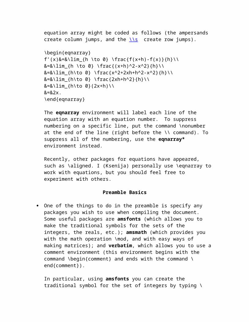
The environments eqnarray and eqnarray* make equations line up nicely on the page. The entries in equation arrays are automatically in math mode; however, the equation array itself must occur in TEXT MODE. A typical equation array might be coded as follows (the ampersands create column jumps, and the \\s create row jumps).

\begin{eqnarray}f’(x)&=&\lim_{h \to 0} \frac{f(x+h)-f(x)}{h}\\&=&\lim_{h \to 0} \frac{(x+h)^2-x^2}{h}\\&=&\lim_{h\to 0} \frac{x^2+2xh+h^2-x^2}{h}\\&=&\lim_{h\to 0} \frac{2xh+h^2}{h}\\&=&\lim_{h\to 0}(2x+h)\\&=&2x.\end{eqnarray}

The eqnarray environment will label each line of the equation array with an equation number. To suppress numbering on a specific line, put the command \nonumber at the end of the line (right before the \\ command). To suppress all of the numbering, use the eqnarray* environment instead.

Recently, other packages for equations have appeared, such as \aligned. I (Ksenija) personally use \eqnarray to work with equations, but you should feel free to experiment with others.

Preamble Basics

One of the things to do in the preamble is specify any packages you wish to use when compiling the document. Some useful packages are amsfonts (which allows you to make the traditional symbols for the sets of the integers, the reals, etc.); amsmath (which provides you with the math operation \mod, and with easy ways of making matrices); and verbatim, which allows you to use a comment environment (this environment begins with the command \begin{comment} and ends with the command \end{comment}).

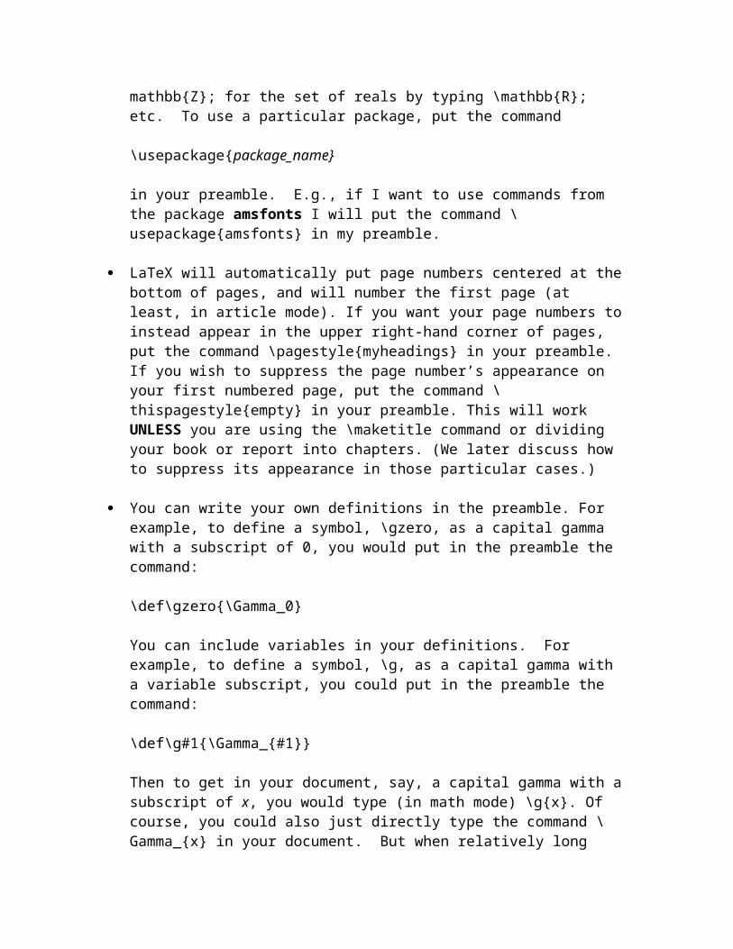
In particular, using amsfonts you can create the traditional symbol for the set of integers by typing \mathbb{Z}; for the set of reals by typing \mathbb{R}; etc. To use a particular package, put the command

\usepackage{package_name}

in your preamble. E.g., if I want to use commands from the package amsfonts I will put the command \usepackage{amsfonts} in my preamble.

LaTeX will automatically put page numbers centered at the bottom of pages, and will number the first page (at least, in article mode). If you want your page numbers to instead appear in the upper right-hand corner of pages, put the command \pagestyle{myheadings} in your preamble. If you wish to suppress the page number’s appearance on your first numbered page, put the command \thispagestyle{empty} in your preamble. This will work UNLESS you are using the \maketitle command or dividing your book or report into chapters. (We later discuss how to suppress its appearance in those particular cases.)

You can write your own definitions in the preamble. For example, to define a symbol, \gzero, as a capital gamma with a subscript of 0, you would put in the preamble the command:

\def\gzero{\Gamma_0}

You can include variables in your definitions. For example, to define a symbol, \g, as a capital gamma with a variable subscript, you could put in the preamble the command:

\def\g#1{\Gamma_{#1}}

Then to get in your document, say, a capital gamma with a subscript of x, you would type (in math mode) \g{x}. Of course, you could also just directly type the

command \Gamma_{x} in your document. But when relatively long commands come up frequently in your document, it can save you a lot of time and typing if you abbreviate the commands with definitions in your preamble. For example, suppose the 3 x 3 identity matrix, I3, over the reals comes up a lot in my document. We will see in a later section that perhaps the easiest way to make this matrix is a command such as the following (using the package amsmath):

\begin{pmatrix}1&0&0\\0&1&0\\0&0&1\end{pmatrix}

What a pain it would be to write this each time that matrix comes up! Instead, you could put the following definition in your preamble:

\def\i3{\begin{pmatrix}1&0&0\\0&1&0\\0&0&1\end{pmatrix}}

Then any time you want to refer to this matrix in the document, you need only type \i3.

You can create commands with more than one variable. For instance, you could create a symbol, \gg, that is a capital gamma with both a variable subscript and a variable superscript:

\def\gg#1#2{\Gamma_{#1}^{#2}}

You could then make, say, a capital gamma with a subscript of 17 and a superscript of 4 by typing:

\gg{17}{4}

Here is a good way of making words appear in roman font in math mode (the way, for example, the commands \gcd and \cos appear in math mode): use the \mathop command. As an example, to define the word Im (for image or imaginary) in this manner, we could make the definition

\def\Im{\mathop{\rm Im}}

Finally, here is a way of making a filled-in box to put at the end of proofs:

\def\qed{{\quad \vrule height 5pt width 5pt depth 0pt}}

With more advanced LaTeX techniques, you can learn create your own symbols in this way.

Titles and Abstracts

You can create title headings using the following commands. A separate title page is created for the document classes book and report; the page will be counted as page 1 if you are using the book class, and as an unnumbered page if you are using the report class. If you are using the document class article, the commands will create a title heading on the first page of your document. These commands should be the FIRST COMMANDS after the \begin{document} command in your file.

\title{title}\author{author(s)}\date{date}

\maketitle

If you omit the \date command, LaTeX will automatically put on the title page the date, according to your computer, of the document’s compilation. You can include more than one author by using the command \and, and you can provide footnotes to authors’ names (or to the title) using the command \thanks. As in the rest of LaTeX, you can force line breaks by using the command \\.

If you wish to suppress the page number’s appearance on the first numbered page, you must put the command \thispagestyle{empty} AFTER your \maketitle command.

For example, see the title heading that the following commands create:

\title{A Guide to \LaTeX}\author{Helmut Kopka\thanks{Does Kopka like lentils?}\\ Max-Planck-Institut\\fur Aeronomie \and Patrick W. Daly \\ I wonder where Daly\\ works? \thanks{Is he a mathematician?}}

\maketitle

Alternatively, you can create title headings using the titlepage environment, which is done by writing \begin{titlepage} title page \end{titlepage}. Using this method, you manually provide your title heading formatting within your titlepage environment text. This time, your title heading will be put on a separate page, regardless of whether you are using the book, report or article document classes. This page will be counted as page 1 if you are using the book class, and as an unnumbered page if you are using the report or article classes.

If you are using the document classes report or article, you can create an abstract using the abstract environment: \begin{abstract} your abstract \end{abstract}. In the report class, the abstract appears on a separate unnumbered page; in the article class, it comes after the title heading on the first page, unless you’ve used the titlepage command to create your title page (in which case it appears at the top of the first page of your

document’s text). You cannot use the abstract environment when using the book document class.

References

To make LaTeX automatically keep track of bibliographic references, use the thebibliography environment (yes, the environment is thebibliography, not bibliography). Identify references within your bibliography with the \bibitem{ID} command. ID represents the name by which you’ll refer to your reference within your document.

For example, the following creates a bibliography with two entries, named G and St:

\begin{thebibliography}{9}

\bibitem{G} Gabriel, P. Auslander-Reiten sequences andrepresentation-finite algebras. Springer-Verlag LNM {\bf 1980,} {\it 831}, 1-71.

\bibitem{St} Stanley, R. P. Structure of incidence algebras and theirautomorphism groups. Bull. Amer. Math. Soc. {\bf 1970,}, {\it 76}, 1236-1239.

\end{thebibliography}

The 9 surely looks mysterious. It is telling LaTeX to indent each entry after the first line by a certain amount. In general, the number you put in the brackets can simply be any number with as many digits as those in the number of bibliographic entries. For example, the label 9 should work if you have 1-9 entries, and the number 99 should work if you have 10 to 99 entries.

To refer to a reference within your document, simply type \cite{ID}, where, again, ID is the entry’s name. For example, I might write in my document:

In \cite{G}, Gabriel discusses blah blah blah . . .

You will need to compile your document twice each time you change something in your bibliography (and sometimes if you change something elsewhere in your document) in order for LaTeX to cite entries correctly.

Tables, Arrays, and Matrices

Tables, arrays, and matrices are all similar to one another (in fact, matrices are specific kinds of arrays). You use tables in text mode, and arrays and matrices in math mode; entries in tables are automatically in text mode, and entries in arrays/matrices are

automatically in math mode. To use the matrix commands, you must load in the amsmath package.

1. Tables

To make a table (remember, to do this you must be in text mode), use the tabular environment:

\begin{tabular}{cols} your table \end{tabular}

In the “cols” brackets you tell LaTeX how many columns you want your table to have, and how you want your entries positioned in each column: l for “left,” c for “center,” and r for “right.” You can also draw vertical lines between your columns by inserting a vertical bar between position entries. For instance, suppose I want my table to have 4 columns, with the entries centered in the first column, right-justified in the second column, and left-justified in the third and fourth columns; suppose further that I want vertical lines separating the first and second columns, and separating the third and fourth columns. I would then use the following code:

\begin{tabular}{c|rl|l} my table \end{tabular}

As in equation arrays, in a table column entries are separated by &s, and rows by \\s. Note that the number of entries in each row must be the same as the number of columns you have specified that your table will have.

For example, what is the table that this command creates?

\begin{tabular}{c|rl|l} ant&bee&cat&dog \\ e&f&g&h \end{tabular}

What about this one?

\begin{tabular}{c|rl|l} ant&bee&cat&dog \\ e&f&g&h \end{tabular}

You can put a horizontal line between rows by typing the command \hline. For example, what is the table that this command creates?

\begin{tabular}{c|rl|l} ant&bee&cat&dog \\ \hline \hline e&f&g&h \\ i&j&k&l \end{tabular}

Of course, you can put math entries in a table by using $s.

For example, what is the table that this command creates?

\begin{tabular}{ccc} ant & bee & $\Gamma_0$ \\ $A\cup B$ & 5 & cat \end{tabular}

2. Arrays

Arrays are pretty much the same as tables, except that you use them in math mode, and by default the array entries are also in math mode. (Note: Equation arrays, which we learned about before, are very similar to arrays. Remember, however, that equation array environments are used in text mode, not math mode.) To make an array, you use the array environment:

\begin{array}{cols} your array \end{array}

Remember this command must be in either inline or display math mode!

Other than using the word array instead of tabular, the syntax for using an array is identical to that for using a table. If you want a roman (that is, non-math mode) word to appear, you can use the command \mbox{ }.

For example, what is the array that this command creates?

\begin{array}{c|rl|l} ant&bee&cat&dog \\ e&f&g&h \end{array}

What about this one?

\begin{array}{c|rl|l} \mbox{ant}&\mbox{bee}&\mbox{cat}&\mbox{dog} \\ e&f&g&h \end{array}

3. Matrices

Matrices form a special class of arrays. To use them, you must load in the amsmath package. You can use the following matrix environments, distinguished by the delimiters that enclose the matrix entries:

pmatrix (for parentheses) bmatrix (for brackets) Bmatrix (for curly braces) vmatrix (for vertical lines) Vmatrix (for double vertical lines).

With you use these commands, you do not specify the number of columns as an argument; the number of columns of the matrix will simply be the number of entries in the longest row you enter into the matrix. (Note that you must enter in the same number of entries in each row of the matrix if you don’t want blank entries to occur.) Other than that, the syntax for creating a matrix is the same as the syntax for creating an array. Like arrays, matrices are used in math mode, and their entries are automatically in math mode.

For example, what is the object that this command creates?

\begin{bmatrix}1&0&2\\ -5 & \pi & \frac{1}{4}\end{bmatrix}

Spacing (in Text Mode)

You can use the commands \hspace{space}, \hspace*{space}, and \hfill to insert blank horizontal spaces, and the commands \vspace{space}, \vspace*{space}, and \vfill to insert blank vertical spaces, in your document. In each command, the argument space is the length specification for the amount of spacing. It can be measured in centimeters (cm), millimeters (mm), inches (in), points (pt), or other units, whose abbreviations are bp, pc, dd, cc, em, and ex. I personally always use the pt length specification.

The \hspace and \hspace* commands put a blank space of width space at the point in the text where it appears. The command \hspace will not add space if it occurs between two lines; the command \hspace* command will insert spacing regardless of where it occurs. The \vspace and \vspace* commands similarly insert vertical space; \vspace will not add space at the beginning of a page, while \vspace* will. The command \hfill (an abbreviation for \hspace{\fill}) inserts enough space wherever it occurs to force the text on either side to be pushed over to the left or right margins. The command \hfill will be ignored if it occurs at the beginning of a line; in that case, you must use the command \hspace*{\fill}. Similarly, the command \vfill inserts enough space wherever it occurs to push text up or down to the upper or lower margins. This command will be ignored if it occurs at the beginning of a page; in that case, you must use the command \vspace*{\fill}.

For example, what is the output of the following?

Birds eat worms.\\ \hspace{2 in} Cats like to \hspace{10pt} chase birds. \hfill Dogs \vfill like to chase cats.

What happens if we turn the first \hspace command into an \hspace* command?

Warning: sometimes LaTeX will want you to put \vspace or \bigskip-type commands on their own lines of code, or even want you to separate them from other lines of code with blank lines, in order for them to be recognized. If it seems like such a command is being ignored by LaTeX, put it on its own line, padded above, below, or above and below by blank lines, and that should do the trick.

Chapters, Sections, Subsections, and Subsubsections†

These commands form a sectioning hierarchy for your document. In the book and report classes, the highest sectioning level is \chapter, followed by \section, \subsection,

† For those who can never have enough subsections!

and finally \subsubsection. In the article class, the highest sectioning level is \section (\chapter is not available for this class), followed by \subsection and then \subsubsection. The resulting physical layout of the divisions of your document depends on which document class you are using.

If you are using the book or report document class and you wish to suppress the page number’s appearance on your first numbered page, you must put the command \thispagestyle{empty} AFTER your first \chapter command.

The syntax for such sectioning commands is demonstrated by the following example:

\chapter{Washing Your Hair}\label{wash}

This will give the chapter the title Washing Your Hair. The label, wash, gives you a way of referring to the chapter number in your text without knowing ahead of time what that number will be. For example, suppose Washing Your Hair is currently in Chapter 3. I could type in my text:

In Chapter 3, we discuss how to wash your hair.

But then suppose I add in another chapter before that chapter, so that now Washing Your Hair is Chapter 4. My reference to that chapter within the text is now incorrect. But if, instead, I had written,

In Chapter \ref{wash}, we discuss how to wash your hair,

then no matter how many chapters I add or delete, the reference will be correct. You may need to compile your document twice in order for your references to be correct.

You may use any combination of letters, numbers, or symbols in your labels. For instance, I may want to have both a chapter and a section that I label as wash. To distinguish between the two, I may choose to label the chapter with the name chap:wash, and the section with the name sec:wash.

There are nuances as to how LaTeX will number your document subdivisions. We may discuss these later in class.

Tables of Contents

To make a table of contents, type \tableofcontents where you want the table to appear. You may need to compile your document twice in order for your table of contents to be

correct. Note: for anything to appear in your table of contents, you will need to have divided your document into chapters or sections.

Numbering Theorems and the Like

Many times it is helpful to have LaTeX automatically keep track of the numbering of theorems, lemmas, corollaries, definitions, examples, etc. You can make this happen by using the \newtheorem command. The \newtheorem command goes in the preamble of your document, and its syntax is as follows:

\newtheorem{struct_type}[num_like]{struct_title}[in_counter]

The square brackets indicate that the num_like and in_counter arguments are optional. struct_type is a keyword with which to refer to that type of structure in your document, and struct_title is the word that is printed in bold face followed by the appropriate number when a structure of that type is called in your document. When I want to insert a structure of type struct_type in my document, I type:

\begin{struct_type} structure \end{struct_type}

For example, I could make the following \newtheorem declaration:

\newtheorem{mythm}{Theorem}

Then I could put the following theorems in my document:

\begin{mythm}If $H$ is a subgroup of finite group $G$, then $|H|$ divides $|G|$. \end{mythm}

\begin{mythm} There are infinitely many prime integers. \end{mythm}

Note that I only needed one \newtheorem declaration for theorems, even if put many theorems in my document.

I could similarly make the \newtheorem declarations

\newtheorem{mylem}{Lemma}\newtheorem{mydef}{Definition}

and put the following lemma and definition in my document:

\begin{mylem} If an integer is divisible by 4, then it is divisible by 2. \end{mylem}

\begin{mydef} A group is said to be {\it abelian} if its operation is commutative.

Perhaps we want these structures to not be labeled completely sequentially, but only sequentially within each chapter. The optional argument in_counter allows us to make this happen. For example, we can make, say, the following declarations:

\newtheorem{mythm}{Theorem}[chapter]\newtheorem{mylem}{Lemma}[chapter]\newtheorem{mydef}{Definition}[chapter]

What happens when we test this out in a document that has been divided into chapters and sections?

Or maybe we want to number theorems along with lemmas, but not with definitions. Then we can use the optional argument num_like, where num_like is the name of an already existing theorem structure whose counter you want to share with that of the structure you’re defining. For example, what happens if we make the following declarations?

\newtheorem{mythm}{Theorem}\newtheorem{mylem}[mythm]{Lemma}\newtheorem{mydef}{Definition}

Or these?

\newtheorem{mythm}{Theorem}[chapter]\newtheorem{mylem}[mythm]{Lemma}\newtheorem{mydef}{Definition}[chapter]

Or these?

\newtheorem{mythm}{Theorem}[chapter]\newtheorem{mylem}[mythm]{Lemma}\newtheorem{mydef}{Definition}

You can also label theorems and the like so that you can refer to them by number later. You do this using the command form:

\begin{struct_type} \label{struct_label} structure \end{struct_type}

Then, if you want to refer to the number of this structure in your document, you type in

\ref{struct_label}

For instance, I could write the following:

\begin{mythm} \label{primethm} There are infinitely many prime integers. \end{mythm}

Then I might write the following in my document:

In Theorem \ref{primethm}, we note that there are infinitely many prime integers.

Again, you may need to compile twice in order for your references to be correct.

Equation Numbering

You can create sequentially numbered equations using the equation environment: \begin{equation} equation \end{equation}. Entries in the equation environment are automatically in math mode; however, the equation itself must occur in TEXT MODE. If your equations are not in chapters (which they of necessity will not be, if you’re in article mode), they will simply be numbered (1), (2), (3), etc., in the order in which they appear in your document. If your equations are in chapters, they will be labeled with labels of the form (x.y), where x is the chapter in which the equation is appearing, and where the equation is the yth equation in that chapter: for instance, if you have two equations in Chapter 1, none in Chapter 2, and four in Chapter 3, your equations will be numbered, in order, as (1.1), (1.2), (3.1), (3.2), (3.3), and (3.4). Equations that occur within the eqnarray environment are numbered within the same scheme as those that occur in the equation environment.

In book, report, or article modes, you may choose to have equation labels also involve section numbers. To do this, use the package amsmath, and in the preamble of your document type in the command:

\numberwithin{equation}{section}

In articles, for instance, if you have two equations in Section 1 and three equations in Section 2, without this command they will be labeled (1), (2), (3), (4), and (5), respectively (remember that articles don’t have chapters); with this command they will be labeled (1.1), (1.2), (2.1), (2.2), and (2.3), respectively. If these equations are in the same sections in Chapter 2 of a book or report, they will be labeled (2.1), (2.2), (2.3), (2.4), and (2.5) without the command, and (2.1.1), (2.1.2), (2.2.1), (2.2.2), and (2.2.3), with it.

You can give equations labels (so that you can reference them in your document) using the command,

\begin{equation} \label{eqn_label} equation \end{equation},

and you can refer to them later by using the command \ref{eqn_label} (note that this is the same command that you use to refer to theorems, lemmas, etc.). As before, you may need to compile twice, to make sure your references are correct.

Defining New Environments

In a previous section, we learned how to use theorem-like environments. Notice that text in those environments is automatically slanted by LaTeX. But perhaps you don’t want the text of your theorems to be slanted. Perhaps you want your theorems automatically centered. Perhaps you want a period appearing after each theorem’s number. You can tailor theorem-like environments (and other environments) to suit your needs using the \newenvironment and \renewenvironment commands. You use the \newenvironment command when defining a new environment, and the \renewenvironment command when redefining an existing environment. These commands go in the preamble of your document, and the basic syntax is as follows:

\newenvironment{env_name}[narg]{beg_def}{end_def}\renewenvironment{env_name}[narg]{beg_def}{end_def}

The argument env_name is the name of your environment, the beg_def argument is the initial text to be inserted when \begin{env_name} is called, and the end_def argument is the final text to be inserted right before \end{env_name} is called. The optional argument narg is a number between 1 and 9 that states how many arguments the environment is to have. (There is also an optional argument opt, but we will not go into that here.)

What happens if I put the following commands in the preamble of my document,

\newtheorem{mythm}{Theorem}

\newenvironment{thm}{\begin{mythm}\begin{upshape}}{\end{upshape}\end{mythm}}

and then write the following theorem:

\begin{thm}If $G$ is a group with prime order, then $G$ is cyclic. \end{thm}

What if I instead define my thm environment as follows?

\newenvironment{thm}{\begin{mythm}{\bf .}}{\end{mythm}}

How can we make the period appear closer to the theorem number? Use the \hspace command, with a negative length measurement!

\newenvironment{thm}{\begin{mythm}\hspace{-5pt}{\bf .}}{\end{mythm}}

Here is an example of a new environment defined with an argument:

\newenvironment{thm}[1]{\begin{mythm}\label{#1}}{\end{mythm}}

What then will this text do?

\begin{thm}{silly.thm}Here is a nonsense theorem.\end{thm}

Graphics

The first thing you will need to do is create and save the image you want to put in your document.

You then include your image in your .tex document in the following way. First, call on the package graphicx: that is, put the command

\usepackage{graphicx}

in your preamble.Then put the code

\includegraphics[scale change]{mypic}

where you want your image to appear. You do not need to put the extension in yourfilename.

The scale change argument in the \includegraphics command is an optional argument that allows you to change the size of your included image. If you want the image to be half as big as its default size, put the command

scale = .5

as your optional argument. If you want your image to be 3 times as big as its default size, what command should you use?

You can center your images by putting them between \begin{center} and \end{center} commands. You can also have them automatically numbered and put attach captions to them using the figure environment. Here is an example of how you would put (and center) a picture in such an environment

\begin{figure}[placement]\begin{center}\includegraphics[scale factor]{mypic}

\caption{$x^2$} \label{polydeg2}\end{center}\end{figure}

The optional argument placement allows you to specify where you would like the figure to appear. The possible arguments are:

1. h (Here) - at the position in the text where the figure environment appears.2. t (Top) - at the top of a text page. 3. b (Bottom) - at the bottom of a text page.4. p (Page of floats) - on a separate float page, which is a page containing no

text, only floats.

The optional argument scale factor allows you to shrink or expand the figure from its default size. If I want the figure to be half its default size, I’d use the argument scale=.5. If I wanted it to be three times its size, what argument would I use?

I can then refer to this figure later in the same way as you refer to theorems or the like: e.g., I can type

Do you like the graph in Figure \ref{polydeg2}?

Some important notes on using figure environments:

The order of your \caption and \label commands here is very important: the \label command must occur after the \caption command. This is kind of annoying, especially since you may not want a caption for your figure! If you don’t want a caption, I still recommend putting in a \caption command with an empty argument, if you want to be sure your labeling will work.

If you want to center images and captions within the figure environment, make sure that, as in the code above, you put your \begin{center} [\end{center}] command immediately after [before] your \begin{figure} [\end{figure}] command.

Finally, as always, if you use labels in these environments, compile twice in order to make sure that your references are correct.

There is a lot more to including graphic images in LaTeX, but hopefully this provides you with a start.