introduction to lectures 1-4. - department of mathematicsschlag/slides/lec0.pdf · pp l2(r) ac...

Introduction to Lectures 1-4.

W. Schlag (University of Chicago)

Maiori, September 2013

W. S. Introduction to Lectures 1-4.

The periodic problem

Consider the periodic second order ODE

− y ′′(x) + V (x)y(x) = Ey(x), E ∈ R (1)

on the line. Assume V (x + L) = V (x) real-valued (may takeL = 1). Then by Floquet theory any solution of (1) is of the formy(x) = e ik(E)xa(x ,E ) where a(x + L,E ) = a(x ,E ). This comesfrom considering the propagator (fundamental matrix) S(L) and itseigenvalues. Since det S(L) = 1, either both eigenvalues lie on theunit circle (and are complex conjugates), or they are real-valuedand reciprocal.What does spec(H) look like, where

(Hy)(x) = −y ′′(x) + V (x)y(x) ?

We need to find those E for which k(E ) is real-valued.


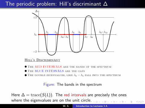
The periodic problem: Hill’s discriminant ∆

Figure: The bands in the spectrum

Here ∆ = trace(S(L)). The red intervals are precisely the oneswhere the eigenvalues are on the unit circle.


The periodic problem

Moreover, the spectrum of H is purely absolutely continuous.Recall: as a self-adjoint operator H on a suitable domain has aspectral resolution N(dE ) so that H =

∫R E N(dE ) which means

that

〈Hf , g〉 =

∫R

E 〈N(dE )f , g〉 ∀ f , g ∈ dom(H)

Lebesgue decomposition: L2(R) = L2(R)pp ⊕ L2(R)ac ⊕ L2(R)sc

orthogonal decomposition into closed subspaces such that themeasure

µf ,g (dE ) = 〈N(dE )f , g〉 ∀ f , g ∈ L2(R)X

is of type X, where X = pp/ac/sc .

How does one identify the spectrum as purely absolutelycontinuous?


Stone formula∀ f , g ∈ L2(R) and any test function ϕ one has

limε→0

1

2πi

∫ ⟨[(H − (λ+ iε))−1 − (H − (λ− iε))−1]f , g

⟩ϕ(λ) dλ

=

∫Rϕ(λ)µf ,g (dλ)

So there is a clear connection between the spectral measure andthe resolvent. For example,

1

πIm (H − (λ+ i0))−1 dλ = Nac(dλ) := N(dλ)�Hac

This is especially useful on the line, since we can compute theresolvent (i.e., Green function) from a fundamental system of (1)(W =Wronskian)

(H − z)−1(x , x ′) =y+(x , z)y−(x ′, z)

W (y+(·, z), y−(·, z))x > x ′

where Im z > 0 and y±(x , z) decay as x → ±∞, respectively.W. S. Introduction to Lectures 1-4.

Physical relevanceIn the early days of quantum mechanics crystals (such as metalsand other electric conductors) were modeled by Schrodingeroperators with periodic potentials. The wave functions areprecisely the Floquet solutions, as noted by Bloch. The fact thatthese “eigenfunctions” are not localized, or extended is interpretedphysically as mobility of the electrons which then translates intoelectric conductivity. Works in any dimension. Mathematicallyspeaking: the spectrum is (absolutely) continuous. Typically, theissue of characterizing singular continuous spectrum is very subtleand many open problems remain (see e.g. Damanik-Killip-Lenz).

In QM it was then an important problem to understand whathappens to a crystal (conductor) if random impurities areintroduced. The common belief was after Bloch that a.c. spectrumis stable and not destroyed. In 1957 Phil Anderson surprisedmany by showing (non-rigorously) that for sufficiently strongrandom, independent potentials on the whole lattice there is onlypure point spectrum and the eigenfunctions decay exponentially.


P. Anderson’s workFor this he received the Nobel prize, since experimentalconfirmation followed. More precisely, consider the randomoperator

H = −∆Zd + λV (2)

on the lattice Zd where V = {vn}n∈Zd with i.i.d. random variablesvn. E.g., take vn = ±1.

d = 1 and any λ 6= 0: pure point spectrum and exponentiallylocalized eigenfunctions (AL). Furstenberg’s theorem onpositive Lyapunov exponents for products of random matricesis the basic mathematical ingredient.d = 2, 3, . . . and LARGE λ 6= 0: AL as shown byFrohlich-Spencer in the 1980s.Conjecture: d = 2 and any λ 6= 0 have AL.Conjecture: d = 3 and SMALL λ 6= 0 have SOME ACSPECTRUM (problem of extended states). In other words,one expects a METAL-INSULATOR PHASE TRANSITIONdepending on the size of the disorder.


Dynamical propertiesIf H exhibits localization, then for any s ≥ 0 one has

supt‖〈x〉se itHψ‖2 <∞

for any ψ ∈ L2. In other words, nothing spreads.Contrast this to the free case: if 〈x〉ψ ∈ L2, then‖〈x〉e it∆ψ‖2 ' 〈t〉. Same for other powers.On the other hand, we have the following behavior on thecontinuous spectrum: for all ψ ∈ L2

c one has

1

T

∫ T

0‖χBe itHψ‖2

2 dt → 0

as T →∞. Here B is any ball. In the free case we have

‖e it∆f ‖∞ ≤ |t|−d/2‖f ‖1

This is the standard dispersive estimate (wave packets of differentfrequencies travel at different speeds).


P. Anderson’s work

Needless to say, all of this is about random potentials in INFINITEVOLUME. Finitely many “impurities” have no effect on theessential spectrum by Weyl’s criterion (on resolvent-compactperturbations of self-adjoint operators).

Anderson’s quote: Localization is a GAME OF RESONANCES.

A resonance here means that on any given finite volume Λ ⊂ Zd

such as alarge cube, and any given energy E the spectrum of therestricted operator H�Λ comes “very close” to E .Of course, one needs to make this quantitative, but the basic ideais to control (or rule out) the presence of long chains of suchresonant cubes. Indeed, if they are present, then the associatedeigenfunction will have equal mass on each of these cubes, andtherefore be extended.Not surprisingly, it is easier to exclude this type of tunneling thanto show that it occurs and leads to infinitely extended states.


The game of resonances

Figure: Resonant cubes


The game of resonances

If we have a periodic structure then there are clearly infinitelyextended periodic chains of cubes which have identical spectrum.So this is what is captured — without any reference to the finitevolume analysis — by Floquet-Bloch solutions in infinite volume.In the random case, we can exploit that disjoint cubes areindependent and thus the probability of having an eigenvalue closeto E in a given cube (which is called “Wegner estimate”) isSQUARED. This essentially leads to the same rapid convergenceas for a Newton scheme in the AL proof at large disorder.

But what if we have strong dependence between the values of thepotential at different sites, such as in quasi-crystals? To be morespecific, suppose vn(x) = F (T nx) where T : X → X is an ergodictransformation on some measure space X 3 x and F : X → R.Here n ∈ Z, in higher dimension can consider the analoguevn(x) = F (T n1

1 ◦ T n22 ◦ . . . ◦ T nd

d x).


Deterministic potentials

Such potentials go by the name of deterministic potentials, and allthe “randomness” sits in the variable x ∈ X . To play the game ofresonances, we clearly have to face the issue of recurrence of thedynamical system. But we need much more (such as a quantitativeergodic theorem) since we must precisely control the smalldivisors which arise in the resolvent (H�Λ− z)−1.

In this generality only have “soft” results such as constancy ofspectrum etc. Any result which requires dealing with small divisorscan only be done with very specific dynamics such as theshift=rotation and very limited potentials (trigonometricpolynomials such as cos, or analytic functions, Gevrey class alsostudied). In many ways, our understanding is very poor.For example, our methods give weaker conclusions forhigher-dimensional shifts, although they should exhibit “morerandomness” and thus the results should be closer to the randomcase – and not further as the current techniques would suggest.


Spectrum of ergodic Schrodinger operators

Consider the self-adjoint operators

(Hxψ)n = ψn+1 + ψn−1 + vn(x)ψn, n ∈ Z

with vn(x) an “ergodic potential”, i.e., vn(x) = V (T nx) andT : X → X ergodic transformation on a probability space X , andV : X → R measurable. Then there exists fixed compact setK ⊂ R with spec(Hx) = K for a.e. x ∈ X . This follows fromergodic theorem and property of the spectral resolution Nx of Hx

Nx = S−1 ◦ NTx ◦ S , S = right translation

In addition, specpp(Hx), specac(Hx), specsc(Hx) are alsodeterministic. Eigenvalues are NOT deterministic, but theirclosure is.Very delicate: Structure of the spectrum such as Cantor set(dense collection of open gaps), versus no gaps.


Basic gap formation resulting from a double resonance,Sinai’s work

Figure: Crossing of graphs of eigenvalues creates a gap

det

(λ1(x)− E ε

ε λ2(x)− E

)= 0, λ1(x0) = λ2(x0) = E0

E±(x) =1

2(λ1(x) + λ2(x))±

√(λ1(x)− λ2(x))2 + 4ε2

(3)

This is a reflection of the fact that for the Dirichlet problemeigenvalues are simple. On the level of eigenfunctions the followingis going on:


Basic mechanism behind gap formation

Figure: Crossing of graphs of eigenvalues create two peaks


Organization of lectures

The goal of these lectures is to present a body of techniques basedon two main ingredients

Estimates for subharmonic functions (Cartan estimate);requires analytic potentials. Basic analytical ingredient whichcontrols the small divisors. The dynamics enters here.

Bounds for semi-algebraic sets. These require polynomialpotentials or such that can be (exponentially) wellapproximated by polynomials. Goal: control the “complexity”(connected components) of “bad sets” in the “randomparameter” x ∈ X to recapture independence of events thatboth x , T nx are “bad” with LARGE n ∈ Z. The specific typeof dynamics enters here, treat on a case-by-case basis. Thissecond step prevents chains of resonant cubes.

Vary the dynamics analytically in a parameter(=frequency/rotation number); eliminate bad frequencies.


OverviewMuch of our presentation is for the basic shift=rotation on thecircle. Parameter equals rotation number and we eliminate a thinset of bad rotation numbers in the process of controlling smalldivisors. We will also make reference to shifts onhigher-dimensional tori, as well as skew shifts. The final Lecture 4is devoted to operators on higher-dimensional lattices.

Lecture 1: subharmonic functions, Riesz representation,transfer matrices, Lyapunov exponent, large deviationestimates, avalanche principle.

Lecture 2: Localization, semi-algebraic sets, elimination ofdouble resonances, positivity of the Lyapunov exponent

Lecture 3: Cartan estimates, derivation of LDT from Cartan,BMO and subharmonic functions, matrix-valued Cartan,splitting lemma

Lecture 4: higher-dimensional lattices, resolvent expansions,applying the matrix-valued Cartan estimate, dealing with largecollections of resonant boxes.


Overview

Many open problems remain, some very basic. Of course, therandom case stands out with the problem of extended states.Appears very difficult. For “deterministic potentials”,higher-dimensional shifts are very poorly understood (gaps in thespectrum?). Endless variations of dynamical systems possible,combine different types of dynamics – for example, mixing withnot mixing: F (x1 + nω, 2nx2)

A basic reference for these lectures is Bourgain’s book “Green’sfunction estimates for lattice Schrodinger operators andapplications”. We do not cover all of it by any means, but gobeyond it in some ways (the higher-dimensional lattices, forexample, or the systematic developments of Cartan estimates). Amajor omission are the KAM applications at the end of Bourgain’sbook aiming at the construction of (quasi)periodic solutions tovarious Hamiltonian wave equations.


References

Anderson, P. Absence of diffusion in certain random lattices. Phys. Rev.109 (1958), 1492–1501.

Aizenman, M., Molchanov, S. Localization at large disorder and atextreme energies: an elementary derivation. Comm. Math. Phys. 157(1993), 245–278.

Bourgain, J. Green’s function estimates for lattice Schrodinger operatorsand applications. Annals of Mathematics Studies, 158. PrincetonUniversity Press, Princeton, NJ, 2005.

Bourgain, J., Goldstein, M. On nonperturbative localization withquasi-periodic potential. Ann. of Math. (2) 152 (2000), no. 3, 835–879.

Damanik, D., Killip, R., Lenz, D. Uniform spectral properties ofone-dimensional quasicrystals. III. α-continuity. Comm. Math. Phys. 212(2000), no. 1, 191–204.

Dinaburg, E. I., Sinai, Y. G. The one dimensional Schrodinger equationwith quasiperiodic potential. Funkt. Anal. i. Priloz. 9 (1975), 8–21.

von Dreifus, H., Klein, A. A new proof of localization in the Andersontight binding model. Comm. Math. Phys. 124 (1989), no. 2, 285–299.


References

Figotin, A., Pastur, L. Spectra of random and almost–periodic operators.Grundlehren der mathematischen Wissenschaften 297, Springer 1992.

Frohlich, J., Spencer, T. Absence of diffusion in the Anderson tightbinding model for large disorder or low energy. Comm. Math. Phys. 88(1983), 151–189.

Frohlich, J., Spencer, T. A rigorous approach to Anderson localization.Phys. Rep. 103 (1984), no. 1–4, 9–25.

Furstenberg, H. Noncommuting random products. Trans. AMS 108(1963), 377–428.

Goldsheid, I. Ya., Molchanov, S. A., Pastur, L. A. A pure point spectrumof the stochastic one-dimensional Schrodinger equation. Funkt. Anal.Appl. 11 (1977), 1–10.

Goldstein, M., Schlag, W. Holder continuity of the integrated density ofstates for quasiperiodic Schrodinger equations and averages of shifts ofsubharmonic functions. Ann. of Math. (2) 154 (2001), no. 1, 155–203.


References

Goldstein, M., Schlag, W. Fine properties of the integrated density ofstates and a quantitative separation property of the Dirichlet eigenvalues.Geom. Funct. Anal. 18 (2008), no. 3, 755–869.

Goldstein, M., Schlag, W. On resonances and the formation of gaps inthe spectrum of quasi-periodic Schrodinger equations. Ann. of Math. (2)173 (2011), no. 1, 337–475.

Jitomirskaya, Svetlana Ya. Almost everything about the almost Mathieuoperator. II. XIth International Congress of Mathematical Physics (Paris,1994), 373–382, Int. Press, Cambridge, MA, 1995.

Last, Y. Almost everything about the almost Mathieu operator. I. XIthInternational Congress of Mathematical Physics (Paris, 1994), 366–372,Int. Press, Cambridge, MA, 1995.

Levin, B. Ya. Lectures on entire functions. Transl. of Math. Monographs,vol. 150. AMS, Providence, RI, 1996.

Sinai, Y. G. Anderson localization for one-dimensional differenceSchrodinger operator with quasi-periodic potential. J. Stat. Phys. 46(1987), 861–909.


introduction to lectures 1-4. - department of mathematicsschlag/slides/lec0.pdf · pp l2(r) ac...

Documents