introduction to machine learningusers.cis.fiu.edu/~jabobadi/cap5610/slides10.pdfintroduction to...

INTRODUCTION TO Machine Learning

2nd Edition

ETHEM ALPAYDIN, modified by Leonardo Bobadilla and some parts fromhttp://www.cs.tau.ac.il/~apartzin/MachineLearning/© The MIT Press, 2010

[email protected]://www.cmpe.boun.edu.tr/~ethem/i2ml2e

Lecture Slides for

Outline

Previous classCh 6: Dimensionality reduction

This class: Ch 6: Dimensionality reductionCh 7: Clustering

Lecture Notes for E Alpaydın 2010 Introduction to Machine Learning 2e © The MIT Press (V1.0)

Outline

Previous classCh 6: Dimensionality reductionCh 7: ClusteringThis class: Ch 6: Dimensionality reduction


CHAPTER 6:

Dimensionality Reduction

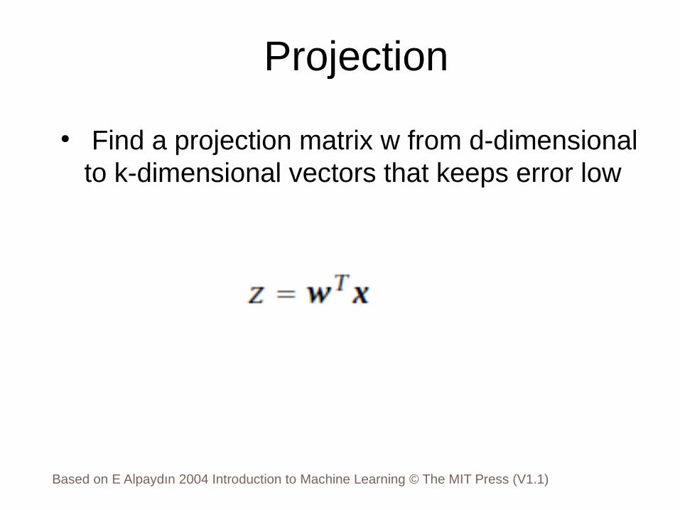
Projection

Based on E Alpaydın 2004 Introduction to Machine Learning © The MIT Press (V1.1)

5

● Find a projection matrix w from d-dimensional to k-dimensional vectors that keeps error low

PCA: Motivation6

● Assume that d observables are linear combination of k<d vectors

● We would like to work with basis as it has lesser dimension and have all(almost) required information

● What we expect from such basis– Uncorrelated or otherwise can be reduced

further– Have large variance or otherwise bear no

information

PCA: Motivation


7

PCA: Motivation


8

● Choose directions such that a total variance of data will be maximum– Maximize Total Variance

● Choose directions that are orthogonal – Minimize correlation

● Choose k<d orthogonal directions which maximize total variance

PCA


9

● Choosing only directions:● ● Maximize variance subject to a constrain using

Lagrange Multipliers

● Taking Derivatives

● Eigenvector. Since want to maximize

we should choose an eigenvector with largest eigenvalue

PCA


10

● d-dimensional feature space● d by d symmetric covariance matrix estimated

from samples ● Select k largest eigenvalue of the covariance

matrix and associated k eigenvectors● The first eigenvector will be a direction with

largest variance

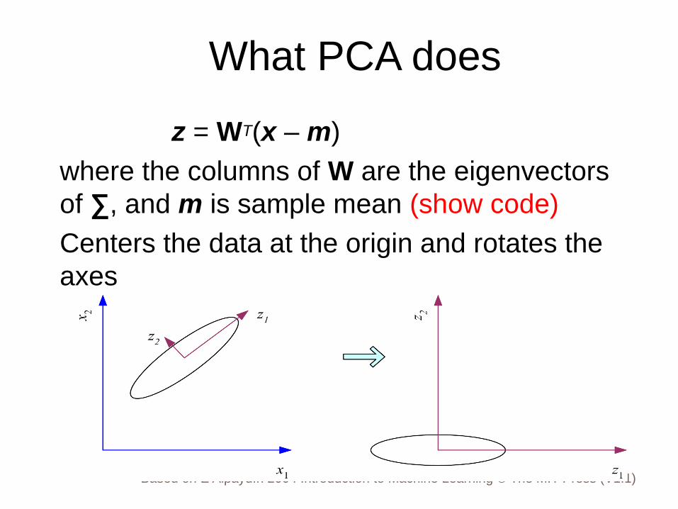
What PCA does


11

z = WT(x – m)

where the columns of W are the eigenvectors of ∑, and m is sample mean (show code)

Centers the data at the origin and rotates the axes

How to choose k ?

Lecture Notes for E Alpaydın 2004 Introduction to Machine Learning © The MIT Press (V1.1)

12

dk

k

λ++λ++λ+λλ++λ+λ

21

21

● Proportion of Variance (PoV) explained

when λi are sorted in descending order ● Typically, stop at PoV>0.9● Scree graph plots of PoV vs k, stop at

“elbow”


13


14

PCA


15

●

● Can take into account classes : Karhuned-Loeve Expansion– Estimate Covariance Per Class– Take average weighted by prior

● Common Principle Components– Assume all classes have same eigenvectors

(directions) but different variances

PCA16

● PCA is unsupervised (does not take into account class information)

● Does not try to explain noise– Large noise can become new dimension/largest

PC

● Interested in resulting uncorrelated variables which explain large portion of total sample variance

Sometimes interested in explained shared variance (common factors) that affect data

Factor Analysis


17

● Assume set of unobservable (“latent”) variables

● Goal: Characterize dependency among observables using latent variables

● Suppose group of variables having large correlation among themselves and small correlation with other variables

● Single factor?

Factor Analysis


18

● Assume k input factors (latent unobservable) variables generating d observables

● Assume all variations in observable variables are due to latent or noise (with unknown variance)

● Find transformation from unobservable to observables which explain the data

Factor Analysis


19

● Find a small number of factors z, which when combined generate x :

xi – µi = vi1z1 + vi2z2 + ... + vikzk + εi where zj, j =1,...,k are the latent factors with

E[ zj ]=0, Var(zj)=1, Cov(zi ,, zj)=0, i ≠ j , εi are the noise sources

E[ εi ]= ψi, Cov(εi , εj) =0, i ≠ j, Cov(εi , zj) =0 ,and vij are the factor loadings

PCA vs FAPCA From x to z z = WT(x –µ )FA From z to x x – µ = Vz + ε

20

x z

z x


Factor Analysis


21

● In FA, factors zj are stretched, rotated and translated to generate x

FA Usage22

● Speech is a function of position of small number of articulators (lungs, lips, tongue)

● Factor analysis: go from signal space (4000 points for 500ms ) to articulation space (20 points)

● Classify speech (assign text label) by 20 points

● Speech Compression: send 20 values

Linear Discriminant Analysis


23

● Find a low-dimensional space such that when x is projected, classes are well-separated

Means and Scatter after projection


24

Good Projection


25

● Means are far away as possible● Scatter is small as possible● Fisher Linear Discriminant

( ) ( ) 2

1 22 21 2

m mJ

s s

−=

+w

26Lecture Notes for E Alpaydın 2010 Introduction to Machine Learning 2e © The MIT Press (V1.0)

Summary


27

● Feature selection– Supervised: drop features which don’t introduce

large errors (validation set)– Unsupervised: keep only uncorrelated features (drop

features that don’t add much information)● Feature extraction

– Linearly combine feature into smaller set of features– Unsupervised

● PCA: explain most of the total variability● FA: explain most of the common variability

– Supervised● LDA: best separate class instances

CHAPTER 7:

Clustering

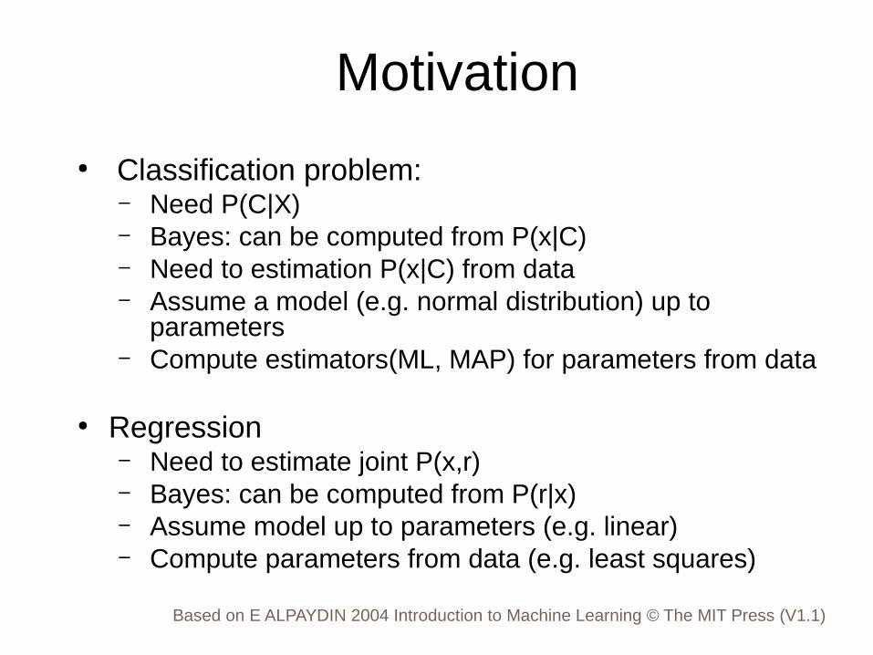
Motivation

Based on E ALPAYDIN 2004 Introduction to Machine Learning © The MIT Press (V1.1)

29

● Classification problem:– Need P(C|X)– Bayes: can be computed from P(x|C) – Need to estimation P(x|C) from data– Assume a model (e.g. normal distribution) up to

parameters– Compute estimators(ML, MAP) for parameters from data

● Regression– Need to estimate joint P(x,r)– Bayes: can be computed from P(r|x)– Assume model up to parameters (e.g. linear)– Compute parameters from data (e.g. least squares)

Motivation


30

● Not always can assume that data came from single distribution/model

● Nonparametric method: don’t assume any model, compute probability of new data directly from old data

● Semi-parametric/mixture models: assume data came from a unknown mixture of known models

Motivation


31

● Optical Character Recognition– Two ways to write 7 (w/o horizontal bar)– Can’t assume single distribution– Mixture of unknown number of templates

● Compared to classification– Number of classes is known– Each training sample has a label of a class– Supervised Learning

Mixture Densities


32

( ) ( ) ( )∑=

=k

iii Ppp

1

| GGxx

● where Gi the components/groups/clusters, P ( Gi ) mixture proportions (priors),p ( x | Gi) component densities

● Gaussian mixture where p(x|Gi) ~ N ( μi , ∑i ) parameters Φ = {P ( Gi ), μi , ∑i }ki=1

unlabeled sample X={xt}t (unsupervised learning)

Example


33

● Check book

Example : Color quantization


34

● Image: each pixels represented by 24 bit color● Colors come from different distribution (e.g. sky,

grass)● Don’t have labeling for each pixels if it’s sky or

grass● Want to use only 256 colors in palette to

represent image as close as possible to original ● Quantize uniformly: assign single color to each

2^24/256 interval● Waste values for rarely occurring intervals

Quantization


35

● Sample (pixels): ● k reference vectors (palette):● Select reference vector for each pixel:

● Reference vectors: codebook vectors or code words

● Compress image● Reconstruction error

jt

jit mxmx −=− min

{ }( )

−=−

=

−= ∑ ∑=

otherwise0

minif 1

1

jt

jit

ti

t i itt

ikii

b

bE

mxmx

mxm X

Encoding/Decoding


36

−=−

=otherwise0

minif 1 jt

jit

tib

mxmx

K-means clustering


37

● Minimize reconstruction error

● Take derivatives and set to zero

● Reference vectors is the mean of all instances it represents

{ }( )1

k t ti i ii t i

E b=

= −∑ ∑m x mX

K-Means clustering


38

● Iterative procedure for finding reference vectors

● Start with random reference vectors● Estimate labels b● Re-compute reference vectors as means ● Continue till converge

k-means Clustering


39

introduction to machine learningusers.cis.fiu.edu/~jabobadi/cap5610/slides10.pdfintroduction to...

Documents