Introduction MAD-X syntax Daily life “Hello World!” example

Introduction to MAD-X

G. Sterbini, CERNThanks to W. Herr and B. Holzer

14 January 2014, ArchampsAnd T. Satogata at USPAS 2017

guido.sterbini@cern.ch

Introduction MAD-X syntax Daily life “Hello World!” example

THE MAD-X LECTURES

We will haveI 1 h lecture (now).I 5 h “hand-on” tutorials (today, tomorrow and on

Thursday).I Today’s tutorial (1 h) will be dedicated to check the pc

remote connections and to prepare a very simple input filefor MADX.

I Tomorrow’s tutorial will be dedicated to explore a FODOcell (1 h) and a FODO lattice (1 h).

I On Thursday we will study a matching cell (1 h) and wewill play with the LHC MADX description (1 h).

Each tutorial is split in two parts of ≈ 30 min (last 10 minutesfor Q&A). Basic knowledge of Windows and Unix is assumedbut do not hesitate to ask in case: we are here to help.

Introduction MAD-X syntax Daily life “Hello World!” example

MAD-X IN 60M:00S!

Introduction

MAD-X syntax

Daily life

“Hello World!” example

Introduction MAD-X syntax Daily life “Hello World!” example

DISCLAIMER. This material is intended to be an introductionto MAD-X: a large part of the code capabilities are notdiscussed in details or are not discussed at all! We will useMAD-X to “visualise” the transverse dynamics concepts.

If you want to deepen the subject you can find a lot ofmaterial on the web (http://mad.web.cern.ch/mad/madx.old/madx_manual.pdf). . .

I googling “madx”, you get the MAD-X homepage.I To wet your appetite, you can google “MAD-X primer”.I To go in details, you can google “MAD-X manual”.

Introduction MAD-X syntax Daily life “Hello World!” example

WHAT IS MAD-X?

I A general purpose beam optics and lattice programdistributed for free by CERN.

I It is used at CERN since more than 20 years for machinedesign and simulation (PS, SPS, LHC, linacs. . . ).

I MAD-X is written in C/C++/Fortran77/Fortran90 (sourcecode is available under CERN copyright).

Introduction MAD-X syntax Daily life “Hello World!” example

A GENERAL PURPOSE BEAM OPTICS CODE

For circular machines, beam lines and linacs. . .

I Describe/document optics parameters from machinedescription.

I Design a lattice for getting the desired properties(matching).

I Simulate beam dynamics, machine imperfections andmachine operation.

Introduction MAD-X syntax Daily life “Hello World!” example

A GENERAL PURPOSE BEAM OPTICS CODE

MAD-X isI multiplatforms (Linux/OSX/WIN. . . ),I very flexible and easy to extend,I made for complicated applications, powerful and rather

complete,I mainly designed for large projects (LEP, LHC, CLIC. . . ).

MAD-X is NOTI a program for teaching,I (very) easy to use for beginners,I coming with a graphical user interface.

Introduction MAD-X syntax Daily life “Hello World!” example

IN LARGE PROJECTS (E.G., LHC):

I Must be able to handle machines with ≥ 104 elements,I many simultaneous MAD-X users (LHC: more than 400

around the world): need consistent database,I if you have many machines: ideally use only one design

program.

Introduction MAD-X syntax Daily life “Hello World!” example

DESCRIBE AN ACCELERATOR IN MAD-X

Goals. . .I Describe, optimize and simulate a machine with several

thousand elements eventually with magnetic elementsshared by different beams, like in colliders.

Define themachinehardware

Definethe beamproperties

Activatethe

sequence

Executethe

operations

Introduction MAD-X syntax Daily life “Hello World!” example

MAD-X LANGUAGE

How does MAD-X get this info? Via text (interpreter).

I It accepts and executes statements, expressions. . . ,I it can be used interactively (input from command line) or

in batch (input from file),I many features of a programming language (loops, if’s,. . . ).

All input statements are analysed by a parser and checked.I E.g. assignments: properties of machine elements, set up of

the lattice, definition of beam properties, errors. . .I E.g. actions: compute lattice functions, optimize and

correct the machine. . .

Introduction MAD-X syntax Daily life “Hello World!” example

MAD-X INPUT LANGUAGE

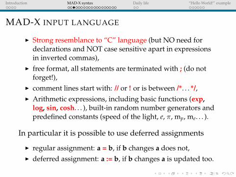
I Strong resemblance to “C” language (but NO need fordeclarations and NOT case sensitive apart in expressionsin inverted commas),

I free format, all statements are terminated with ; (do notforget!),

I comment lines start with: // or ! or is between /*. . . */,I Arithmetic expressions, including basic functions (exp,

log, sin, cosh. . . ), built-in random number generators andpredefined constants (speed of the light, e, π, mp, me. . . ).

In particular it is possible to use deferred assignments

I regular assignment: a = b, if b changes a does not,I deferred assignment: a := b, if b changes a is updated too.

Introduction MAD-X syntax Daily life “Hello World!” example

EXAMPLE: DEFERRED ASSIGNMENTS

We use the value command to print the variables content.

Introduction MAD-X syntax Daily life “Hello World!” example

DEFINITIONS OF THE LATTICE ELEMENTS

Generic pattern to define an element:label: keyword, properties. . . ;

I For a dipole magnet:MBL: SBEND, L=10.0;

I For a quadrupole magnet:MQ: QUADRUPOLE, L=3.3;

I For a sextupole magnet:MSF: SEXTUPOLE, L=1.0;

In the previous examples we considered only the L property,that is the length in meters of the element.

Introduction MAD-X syntax Daily life “Hello World!” example

THE STRENGTH OF THE ELEMENTS

The name of the parameter that define the normalizedmagnetic strength of the element depends on the element type.

I For dipole (horizontal bending) magnet is k0:

k0 = 1BρBy

[in m−1]

I For quadrupole magnet is k1:

k1 = 1Bρ

∂By∂x

[in m−2]

I For sextupole magnet is k2:

k2 = 1Bρ

∂2By

∂x2

[in m−3]

Introduction MAD-X syntax Daily life “Hello World!” example

INTERLUDE

What does k1 mean? It is related to the quad focal length 1.

1k1 Lquad

= f (1)

Assuming k1 = 10−1 m and Lquad = 10−1 m the f = 102 m.

f

k1, Lquad

1thin lens approximation

Introduction MAD-X syntax Daily life “Hello World!” example

EXAMPLE: DEFINITIONS OF ELEMENTS

I Sextupole magnet:ksf = 0.00156;MSF: SEXTUPOLE, K2 = ksf, L=1.0;

I Multipole magnet ”thin” element:MMQ: MULTIPOLE, KNL = {k0 · l, k1 · l, k2 · l, k3 · l, . . . };

I LHC dipole magnet as thick element:length = 14.3;p = 7000;angleLHC = 8.33 * clight * length/p;MBL: SBEND, ANGLE = angleLHC;

Introduction MAD-X syntax Daily life “Hello World!” example

THE LATTICE SEQUENCE

A lattice sequence is an ordered collection of machine elements.Each element has a position in the sequence that can be definedwrt the CENTRE, EXIT or ENTRY of the element and wrt thesequence start or the position of an other element:

label: SEQUENCE, REFER=CENTRE, L=length;. . . ;. . . ;. . . here specify position of all elements. . . ;. . . ;. . . ;ENDSEQUENCE;

Introduction MAD-X syntax Daily life “Hello World!” example

EXAMPLE OF SEQUENCE: LHC (TOO TOUGH?)

Introduction MAD-X syntax Daily life “Hello World!” example

BEAM DEFINITION & SEQUENCE ACTIVATION

Generic pattern to define the beam:label: BEAM, PARTICLE=x, ENERGY2=y,. . . ;e.g., BEAM, PARTICLE=proton, ENERGY=7000;//in GeV

After a sequence has been read, it can be activated:USE, SEQUENCE=sequence label;e.g., USE, SEQUENCE=lhc1;The USE command expands the specified sequence, inserts thedrift spaces and makes it active.

2It is the TOTAL energy!

Introduction MAD-X syntax Daily life “Hello World!” example

DEFINITION OF OPERATIONS

Once the sequence is activated we can perform operations on it.

I Calculation of Twiss parameters around the machine (veryimportant) in order to know, for stable sequences, theirmain optical parameters.TWISS, SEQUENCE=sequence label;//periodic solutionTWISS, SEQUENCE=sequence label, betx=1;//IC solution

I Production of graphical output of the main opticalfunction (e.g., β-functions):PLOT, HAXIS=s, VAXIS=betx,bety;

ExampleTWISS, SEQUENCE=juaseq, FILE=twiss.out;PLOT, HAXIS=s, VAXIS=betx, bety, COLOUR=100;

Introduction MAD-X syntax Daily life “Hello World!” example

EXAMPLE OF THE TWISS FILE

* NAME S BETX BETY$ %s %le %le %le"QF" 1.5425 107.5443191 19.4745051"QD" 33.5425 19.5134888 107.4973054"QF" 65.5425 107.5443191 19.4745051"QD" 97.5425 19.5134888 107.4973054"QF" 129.5425 107.5443191 19.4745051"QD" 161.5425 19.5134888 107.4973054"QF" 193.5425 107.5443191 19.4745051"QD" 225.5425 19.5134888 107.4973054"QF" 257.5425 107.5443191 19.4745051"QD" 289.5425 19.5134888 107.4973054"QF" 321.5425 107.5443191 19.4745051"QD" 353.5425 19.5134888 107.4973054"QF" 385.5425 107.5443191 19.4745051"QD" 417.5425 19.5134888 107.4973054"QF" 449.5425 107.5443191 19.4745051"QD" 481.5425 19.5134888 107.4973054"QF" 513.5425 107.5443191 19.4745051"QD" 545.5425 19.5134888 107.4973054"QF" 577.5425 107.5443191 19.4745051"QD" 609.5425 19.5134888 107.4973054........

Introduction MAD-X syntax Daily life “Hello World!” example

EXAMPLE OF THE GRAPHICAL OUTPUT (PS FORMAT)

1000. 1200. 1400. 1600. 1800. 2000. 2200.Momentum offset = 0.00 %

s (m)

s Periodic horizontal beta function

25.30.35.40.45.50.55.60.65.70.75.80.85.90.

x(m

)

Introduction MAD-X syntax Daily life “Hello World!” example

MATCHING GLOBAL PARAMETERSIt is possible to modify the optical parameters of the machineusing the MATCHING module of MAD-X.

I Adjust magnetic strengths to get desired properties (e.g.,tune Q, chromaticity dQ),

I Define the properties to match and the parameters to vary.

Example:MATCH, SEQUENCE=sequence name;

GLOBAL, Q1=26.58;//H-tuneGLOBAL, Q2=26.62;//V-tuneVARY, NAME= kqf, STEP=0.00001;VARY, NAME = kqd, STEP=0.00001;LMDIF, CALLS=50, TOLERANCE=1e-6;//method adopted

ENDMATCH;

Introduction MAD-X syntax Daily life “Hello World!” example

OTHER TYPES OF MATCHING I

Local matching and performance matching:

I Local optical functions (insertions, local optics change),I any user defined variable.

1000. 1200. 1400. 1600. 1800. 2000. 2200.Momentum offset = 0.00 %

s (m)

s Periodic horizontal beta function

25.30.35.40.45.50.55.60.65.70.75.80.85.90.

x(m

)

1000. 1200. 1400. 1600. 1800. 2000. 2200.Momentum offset = 0.00 %

s (m)

s Horizontal beta with low beta insertion

0.0

100.

200.

300.

400.

500.

600.

700.

800.

900.

x(m

)

x

.

Introduction MAD-X syntax Daily life “Hello World!” example

OTHER TYPES OF MATCHING II

Local matching and performance matching:

I Local optical functions (insertions, local optics change),I any user defined variable.

Example:MATCH, SEQUENCE=sequence name;

CONSTRAINT, range=#e, BETX=50;CONSTRAINT, range=#e, ALFX=-2;VARY, NAME= kqf, STEP=0.00001;VARY, NAME = kqd, STEP=0.00001;JACOBIAN, CALLS=50, TOLERANCE=1e-6;

ENDMATCH;

Introduction MAD-X syntax Daily life “Hello World!” example

GENERAL CONSIDERATIONS ON MAD-X SYNTAX

Input language seems heavy, but:

I can be interfaced to data base and to other programs (e.g.,MathematicaTM, MatlabTM. . . ),

I programs exist to generate the input interactively,I allows web based applications,I allows interface to operating system.

MAD-X can estimate the machine performance by:

I studying of long term stability with multipolar component,I taking into account the tolerances for machine elements,I simulating operation of the machine (imperfections,. . . ).

Introduction MAD-X syntax Daily life “Hello World!” example

DO WE USE MAD-X FOR EVERYTHING? NO!

MAD-X is an optics program (single particle dynamics).

MAD-X has limitations whereI multi particle and multi bunch simulations are required,I machine is not static, i.e., beam changes its own

environment (space charge, instabilities, beam-beameffects. . . ),

I requires self-consistent treatment, computation of fieldsand forces,

I execution speed is an issue,I for detailed studies dedicated programs are needed, but

often with I/O interface to MAD-X.

Introduction MAD-X syntax Daily life “Hello World!” example

SOME USEFUL TIPS FOR THE TUTORIALS (WIN)

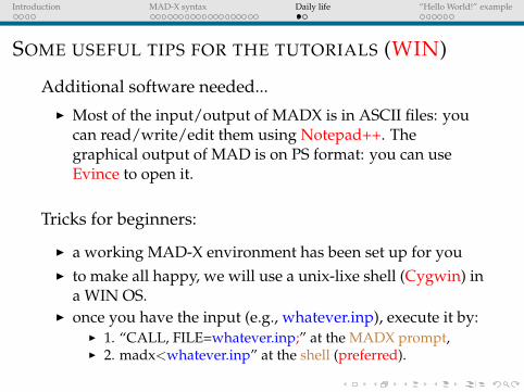
Additional software needed...I Most of the input/output of MADX is in ASCII files: you

can read/write/edit them using Notepad++. Thegraphical output of MAD is on PS format: you can useEvince to open it.

Tricks for beginners:

I a working MAD-X environment has been set up for youI to make all happy, we will use a unix-lixe shell (Cygwin) in

a WIN OS.I once you have the input (e.g., whatever.inp), execute it by:

I 1. “CALL, FILE=whatever.inp;” at the MADX prompt,I 2. madx<whatever.inp” at the shell (preferred).

Introduction MAD-X syntax Daily life “Hello World!” example

ACCESS REMOTE MACHINE JUASXX

I Computer: JUASXXI User: JUASXX\ juasuserI PWD: Juas2012UserI Cygwin (UNIX shell in

WIN). From the shell withthe command “open” youopen the Win Explorer(edit inp, read out)

I Use your assigned PC!

Introduction MAD-X syntax Daily life “Hello World!” example

“HELLO WORLD!” INPUT FILE

Introduction MAD-X syntax Daily life “Hello World!” example

“HELLO WORLD!” OUTPUT (1)

Introduction MAD-X syntax Daily life “Hello World!” example

“HELLO WORLD!” OUTPUT (2)

Introduction MAD-X syntax Daily life “Hello World!” example

“HELLO WORLD!” OUTPUT (3)

Introduction MAD-X syntax Daily life “Hello World!” example

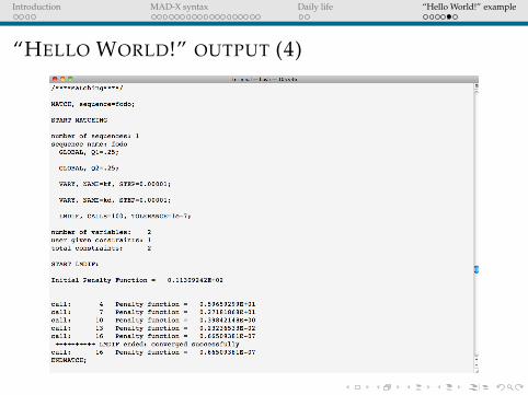
“HELLO WORLD!” OUTPUT (4)

Introduction MAD-X syntax Daily life “Hello World!” example

“HELLO WORLD!” OUTPUT (5)

Tutorial 1 Tutorial 2 Tutorial 3 Tutorial 4 Tutorial 5

TUTORIAL 1: FIRST PART

My first MADX job.

1. Connect to the remote machine assigned to your pc station(JuasXX).

2. Open a Cygwin terminal and make and move to a newfolder.

3. Open an editor and write your first MADX input file (just 1line like “stop;” or “exit;” or “quit;”).

4. Run it. If all is fine, nothing interesting should happen.

Tutorial 1 Tutorial 2 Tutorial 3 Tutorial 4 Tutorial 5

TUTORIAL 1: SECOND PART

My first accelerator.

1. Make a very simple machine with 2 quads (focusing anddefocusing). Each quad is L=0.1 m long and has a focallength of f=20 m (K1×L=1/f in thin lens approximation).

2. Build a sequence of 4 m putting the center of the quads at 1and 3 m.

3. Define a proton beam at Etot = 2 GeV. Activate thesequence, try to find the periodic solution and plot theβ-functions. If you found βmax ≈ 43 m you succeeded. Trywith Etot = 0.7 GeV.

4. Using the plot you obtained can you estimate the phaseadvance of the cell?

Tutorial 1 Tutorial 2 Tutorial 3 Tutorial 4 Tutorial 5

TUTORIAL 2: FIRST PART

Build a simplified LHC FODO cell.

I The LHC FODO cell is long 106.9 m. Each quad is ≈ 5.3 m.Build the cell in MADX putting the start of the first quad atthe start of the sequence.

I Define the beam (proton at Etot = 7 TeV), activate thesequence and try to twiss it powering the quads to obtain∆µ ≈ 90 deg phase advance in the cell using the thin lensapproximation (use Fig. 1). What is the actual phaseadvance computed by MADX?

Tutorial 1 Tutorial 2 Tutorial 3 Tutorial 4 Tutorial 5

TUTORIAL 2: FIRST PART

0 0.5 1 1.5 2 2.5 3 3.5 40

0.1

0.2

0.3

0.4

0.5

0.6

0.7

0.8

0.9

1

∆µ/π

[rad

]

K1 Lcell

Lquad

[−]

Figure 1: Phase advance versus quad strength, cell length and quadlength. Thin lens approximation of a FODO.

Tutorial 1 Tutorial 2 Tutorial 3 Tutorial 4 Tutorial 5

TUTORIAL 2: SECOND PART

Build a simplified LHC FODO cell.

I What is the βmax? Compare with the thin lensapproximation (Fig. 2). And the maximum beam σ(assume εn=3 mrad mm, Etot = 7 TeV).

I If you increase the focusing strength of the quadrupole,what is the effect of it on the βmax, βmin and on the ∆µ?

Tutorial 1 Tutorial 2 Tutorial 3 Tutorial 4 Tutorial 5

TUTORIAL 2: SECOND PART

1 1.5 2 2.5 3 3.5 40

0.5

1

1.5

2

2.5

3

3.5

4

4.5

5

[−]

K1 Lcell

Lquad

[−]

βmax

Lcell

βmin

Lcell

Figure 2: β-functions versus quad strength, cell length and quadlength. Thin lens approximation of a FODO.

Tutorial 1 Tutorial 2 Tutorial 3 Tutorial 4 Tutorial 5

TUTORIAL 3: FIRST PART

The LHC FODO lattice

I Consider now that in the cell of Tutorial 2 there are 4 sectordipoles of 14.3 m. In the lattice there are a total of 736dipoles with equal bending angles. Install the four dipolesin the FODO cell. Do the dipoles (weak focusing) affect onthe βmax and the dispersion? Compute the relativevariation on the βmax on the two planes.

I LHC has 8 octants, each one of 23 FODO cells. What is thephase advance contribution due to the octants in LHC?

Tutorial 1 Tutorial 2 Tutorial 3 Tutorial 4 Tutorial 5

TUTORIAL 3: SECOND PART

Changing the machine working point.

I Change the beam to Etot = 3.5 TeV. What is the new tune ofthe machine? Why?

I Suppose you want to set a tune of (60.2, 67.2), match theFODO to get it. What is the maximum tune that you canreach with 23 cells/octant and 8 octants? (HINT: what itthe maximum phase advance per FODO cell in thinapproximation?...)

Tutorial 1 Tutorial 2 Tutorial 3 Tutorial 4 Tutorial 5

TUTORIAL 4: FIRST PART

Periodic solution and IC solutionI Build a transfer line of 10 m with 4 quads of L=0.4 m

(centered at 2, 4, 6, and 8 m). With K1 respectively of 0.1,0.1 , 0.1 , 0.1 m−2. Can you find a periodic solution?

I Can you find a IC solution starting from(βx, αx, βy, αy) = (1, 0, 2, 0)?

I What is the final optical condition (βendx , αend

x , βendy , αend

y )?

Tutorial 1 Tutorial 2 Tutorial 3 Tutorial 4 Tutorial 5

TUTORIAL 4: SECOND PART

Periodic solution and IC solutionI Starting from (βx, αx, βy, αy) = (1, 0, 2, 0) match the line to

(βx, αx, βy, αy) = (2, 0, 1, 0) at the end.I Starting from (βx, αx, βy, αy) = (1, 0, 2, 0) and the gradient

obtained with the previous matching, match to(βend

x , αendx , βend

y , αendy ). Can you find back K1 respectively of

0.1, 0.1 , 0.1 , 0.1 m−2?I consider that the quadrupoles have an excitation current

factor of 100 A/m2 and an excitation magnetic factor of 100T/m/A and aperture of 40 mm diameter. Compute themagnetic field at the poles of the four quads after matching(HINT: assume linear regime and use a dimensionalapproach).

Tutorial 1 Tutorial 2 Tutorial 3 Tutorial 4 Tutorial 5

TUTORIAL 5: FIRST PART

LHC and MADXI Run the MADX scripts.I What is the LHC length? What is the s-position of IP1 and

IP5? and the β-functions there?I What are the beam1 and beam2 tunes at injections?

Tutorial 1 Tutorial 2 Tutorial 3 Tutorial 4 Tutorial 5

TUTORIAL 5: SECOND PART

LHC and MADXI Are the two beams colliding in IP1 at injection?I Is the crossing of the two beams vertical or horizontal in

IP1 at collision?I What are the beta function at the IPs at collision energy?

Why do we inject with a higher β-function at the IPs?