introduction to madx - wikis · introduction to madx werner herr, cern, ... general purpose lattice...
TRANSCRIPT

Introduction to MADX
Werner Herr, CERN, BE Department
For all MAD details:
(http://cern.ch/mad)
see also:
MADX primer
Werner Herr, MAD introduction, CAS 2009, Darmstadt

Where you find all that:
Documentation: /media/usbdisk/doc
Examples in: /media/usbdisk/examples
Executable:
/media/usbdisk/bin/madx (LINUX)
/media/usbdisk/exe/madx (WINDOWS)
Source code in: /media/usbdisk/madX
Everything also at:
http://cern.ch/Werner.Herr/CAS2009
Werner Herr, MAD introduction, CAS 2009, Darmstadt

MADX - part 1
Description of the basic concepts and
the language
Compute optical functions
Get the parameters you want
Beam dimensions
Tune, chromaticity

MADX - part 2
Machines with imperfections and
corrections
Design of insertions
Dispersion suppressor
Low β insertion
Particle tracking

General purpose lattice programs
For circular machines or linacs
Calculate optics parameters from machine
description
Compute (match) desired quantities
Simulate and correct machine imperfections
Simulate beam dynamics
Used in this course: MADX

What is MADX ?
The latest version in a long line of development
Used at CERN since more than 20 years for
machine design and simulation (PS, SPS, LEP,
LHC, future linacs, beam lines)
(still) Existing versions:
MAD8, MAD9, MADX (version 4, with PTC)
Mainly designed for large projects (LEP, LHC,
CLIC ..)

Why we use MADX here ?
This is not a large project, but:
Multi purpose:
From early design to final evaluation
Running on all systems
Source is free and easy to extend
Input easy to understand
Easy to understand what is happening:
No hidden or invisible actions or computations
Every computational step is explicit

Data required by an optics program ?
Description of the machine:
Definition of each machine element
Attributes of the elements
Positions of the elements
Description of the beam(s)
Directives (what to do ?)
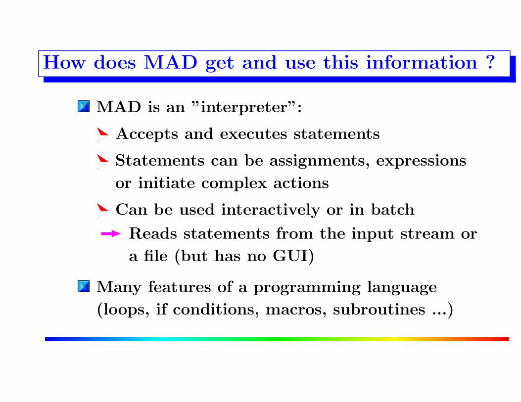
How does MAD get and use this information ?
MAD is an ”interpreter”:
Accepts and executes statements
Statements can be assignments, expressions
or initiate complex actions
Can be used interactively or in batch
Reads statements from the input stream or
a file (but has no GUI)
Many features of a programming language
(loops, if conditions, macros, subroutines ...)

MAD input language
Strong resemblance to ”C” language
All statements are terminated with ;
Comment lines start with: // or !
Arithmetic expressions, including basic functions (exp,
log, sin, cosh ...)
In-built random number generators for various
distributions
Deferred expressions (:= instead of =)
Predefined constants (clight, e, pi, mp, me ...)

MADX conventions
Not case sensitive
Elements are placed along the reference orbit
(variable s)
Horizontal (assumed bending plane) and
vertical variables are x and y
Describes a local coordinate system moving
along s
i.e. x = y = 0 follows the curvilinear system

More conventions
MAD variables are floating point numbers (double
precision)
Variables can be used in expressions:
ANGLE = 2*PI/NBEND;
AIP = ATAN(SX1/SX2);
The assignment symbols = and := have a very different
behaviour (here random number generator)!
DX = GAUSS()*1.5E-3;
The value is computed once and kept in DX
DX := GAUSS()*1.5E-3;
The value is recomputed every time DX is used

Try it ..
> madx
X: ==> angle = 2*pi/1232;
X: ==> value, angle;
X: ==> value,asin(1.0)*2;
X: ==> dx = gauss()*2.0;
X: ==> value, dx;
X: ==> value, dx;
X: ==> dx := gauss()*2.0;
X: ==> value, dx;
X: ==> value, dx;

Try it ..
if you store everything in a file: my.file
> madx
X: ==> call, file=my.file;
> madx
X: ==> (cut and paste, e.g. from another window ..)
> madx < my.file (LINUX)

MAD input statements
Typical assignments:
� � � � � � � � � � � � � � �� � � � � � � � � � � � � � �� � � � � � � � � � � � � � �� � � � � � � � � � � � � � �� � � � � � � � � � � � � � �� � � � � � � � � � � � � � �� � � � � � � � � � � � � � �� � � � � � � � � � � � � � �� � � � � � � � � � � � � � �� � � � � � � � � � � � � � �� � � � � � � � � � � � � � �� � � � � � � � � � � � � � �� � � � � � � � � � � � � � �� � � � � � � � � � � � � � �� � � � � � � � � � � � � � �� � � � � � � � � � � � � � �� � � � � � � � � � � � � � �� � � � � � � � � � � � � � �� � � � � � � � � � � � � � �� � � � � � � � � � � � � � �� � � � � � � � � � � � � � �� � � � � � � � � � � � � � �� � � � � � � � � � � � � � �� � � � � � � � � � � � � � �� � � � � � � � � � � � � � �� � � � � � � � � � � � � � �� � � � � � � � � � � � � � �� � � � � � � � � � � � � � �� � � � � � � � � � � � � � �� � � � � � � � � � � � � � �� � � � � � � � � � � � � � �� � � � � � � � � � � � � � �� � � � � � � � � � � � � � �� � � � � � � � � � � � � � �� � � � � � � � � � � � � � �� � � � � � � � � � � � � � �� � � � � � � � � � � � � � �� � � � � � � � � � � � � � �� � � � � � � � � � � � � � �� � � � � � � � � � � � � � �
Properties of machine elements
� � � � � � � � � � � � � � �� � � � � � � � � � � � � � �� � � � � � � � � � � � � � �� � � � � � � � � � � � � � �� � � � � � � � � � � � � � �� � � � � � � � � � � � � � �� � � � � � � � � � � � � � �� � � � � � � � � � � � � � �� � � � � � � � � � � � � � �� � � � � � � � � � � � � � �� � � � � � � � � � � � � � �� � � � � � � � � � � � � � �� � � � � � � � � � � � � � �� � � � � � � � � � � � � � �� � � � � � � � � � � � � � �� � � � � � � � � � � � � � �� � � � � � � � � � � � � � �� � � � � � � � � � � � � � �� � � � � � � � � � � � � � �� � � � � � � � � � � � � � �� � � � � � � � � � � � � � �� � � � � � � � � � � � � � �� � � � � � � � � � � � � � �� � � � � � � � � � � � � � �� � � � � � � � � � � � � � �� � � � � � � � � � � � � � �� � � � � � � � � � � � � � �� � � � � � � � � � � � � � �� � � � � � � � � � � � � � �� � � � � � � � � � � � � � �� � � � � � � � � � � � � � �� � � � � � � � � � � � � � �� � � � � � � � � � � � � � �� � � � � � � � � � � � � � �� � � � � � � � � � � � � � �� � � � � � � � � � � � � � �� � � � � � � � � � � � � � �� � � � � � � � � � � � � � �� � � � � � � � � � � � � � �� � � � � � � � � � � � � � �
Set up of the lattice
� � � � � � � � � � � � � � �� � � � � � � � � � � � � � �� � � � � � � � � � � � � � �� � � � � � � � � � � � � � �� � � � � � � � � � � � � � �� � � � � � � � � � � � � � �� � � � � � � � � � � � � � �� � � � � � � � � � � � � � �� � � � � � � � � � � � � � �� � � � � � � � � � � � � � �� � � � � � � � � � � � � � �� � � � � � � � � � � � � � �� � � � � � � � � � � � � � �� � � � � � � � � � � � � � �� � � � � � � � � � � � � � �� � � � � � � � � � � � � � �� � � � � � � � � � � � � � �� � � � � � � � � � � � � � �� � � � � � � � � � � � � � �� � � � � � � � � � � � � � �� � � � � � � � � � � � � � �� � � � � � � � � � � � � � �� � � � � � � � � � � � � � �� � � � � � � � � � � � � � �� � � � � � � � � � � � � � �� � � � � � � � � � � � � � �� � � � � � � � � � � � � � �� � � � � � � � � � � � � � �� � � � � � � � � � � � � � �� � � � � � � � � � � � � � �� � � � � � � � � � � � � � �� � � � � � � � � � � � � � �� � � � � � � � � � � � � � �� � � � � � � � � � � � � � �� � � � � � � � � � � � � � �� � � � � � � � � � � � � � �� � � � � � � � � � � � � � �� � � � � � � � � � � � � � �� � � � � � � � � � � � � � �� � � � � � � � � � � � � � �
Definition of beam properties (particle type,
energy, emittance ...)
� � � � � � � � � � � � � � �� � � � � � � � � � � � � � �� � � � � � � � � � � � � � �� � � � � � � � � � � � � � �� � � � � � � � � � � � � � �� � � � � � � � � � � � � � �� � � � � � � � � � � � � � �� � � � � � � � � � � � � � �� � � � � � � � � � � � � � �� � � � � � � � � � � � � � �� � � � � � � � � � � � � � �� � � � � � � � � � � � � � �� � � � � � � � � � � � � � �� � � � � � � � � � � � � � �� � � � � � � � � � � � � � �� � � � � � � � � � � � � � �� � � � � � � � � � � � � � �� � � � � � � � � � � � � � �� � � � � � � � � � � � � � �� � � � � � � � � � � � � � �� � � � � � � � � � � � � � �� � � � � � � � � � � � � � �� � � � � � � � � � � � � � �� � � � � � � � � � � � � � �� � � � � � � � � � � � � � �� � � � � � � � � � � � � � �� � � � � � � � � � � � � � �� � � � � � � � � � � � � � �� � � � � � � � � � � � � � �� � � � � � � � � � � � � � �� � � � � � � � � � � � � � �� � � � � � � � � � � � � � �� � � � � � � � � � � � � � �� � � � � � � � � � � � � � �� � � � � � � � � � � � � � �� � � � � � � � � � � � � � �� � � � � � � � � � � � � � �� � � � � � � � � � � � � � �� � � � � � � � � � � � � � �� � � � � � � � � � � � � � �
Assignment of errors and imperfections
Typical actions:
Compute lattice functions
Correct machines

Definitions of machine elements
All machine elements have to be described
Can be described individually
Can be described as a family (CLASS) of
elements, i.e. all elements with the same
attributes
All elements can have unique names ( .. but
don’t have to)
Definitions can be used in subsequent
commands and statements

How to define machine elements ?
MAD-X Keywords used to define the type of an
element.
Can define single element or class of elements
and give it a name
General format:
name: keyword, attributes;
Some examples:

Example: definitions of elements
To assign attributes to machine elements
Dipole (bending) magnet:
MBL: SBEND, L=10.0, ANGLE = 0.0145444;
Quadrupole magnet:
MQ: QUADRUPOLE, L=3.3, K1 = 1.23E-02;
Sextupole magnet:
ksf = 0.00156;
MSF: SEXTUPOLE, K2 := ksf , L=1.0;
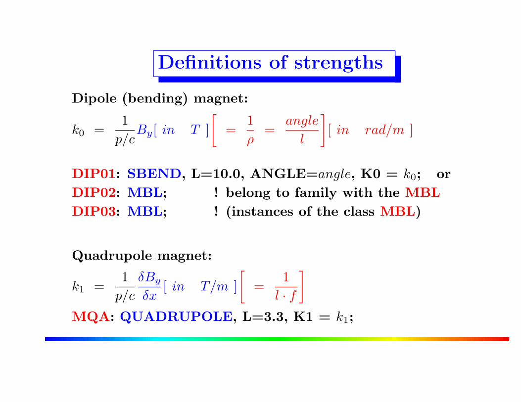
Definitions of strengths
Dipole (bending) magnet:
k0 =1
p/cBy[ in T ]
[
=1
ρ=
angle
l
]
[ in rad/m ]
DIP01: SBEND, L=10.0, ANGLE=angle, K0 = k0; or
DIP02: MBL; ! belong to family with the MBL
DIP03: MBL; ! (instances of the class MBL)
Quadrupole magnet:
k1 =1
p/c
δBy
δx[ in T/m ]
[
=1
l · f
]
MQA: QUADRUPOLE, L=3.3, K1 = k1;

Definitions of strengths
Sextupole magnet:
k2 =1
p/c
δ2By
δx2
[
in T/m2]
KLSF = k2;
MSXF: SEXTUPOLE, L=1.1, K2 = KLSF;
Octupole magnet:
k3 =1
p/c
δ3By
δx3
[
in T/m3]
KLOF = k3;
MOF: OCTUPOLE, L=1.1, K3 = KLOF;

Example: definitions of elements
LHC dipole magnet:
length = 14.3;
B = 8.33;
PTOT = 7.0E12;
ANGLHC = B * clight * length/PTOT;
MBLHC: SBEND, L = Length, ANGLE = anglhc;
ANGLHC = 2*pi/1232;
MBLHC: SBEND, L = LENGTH, ANGLE = ANGLHC;
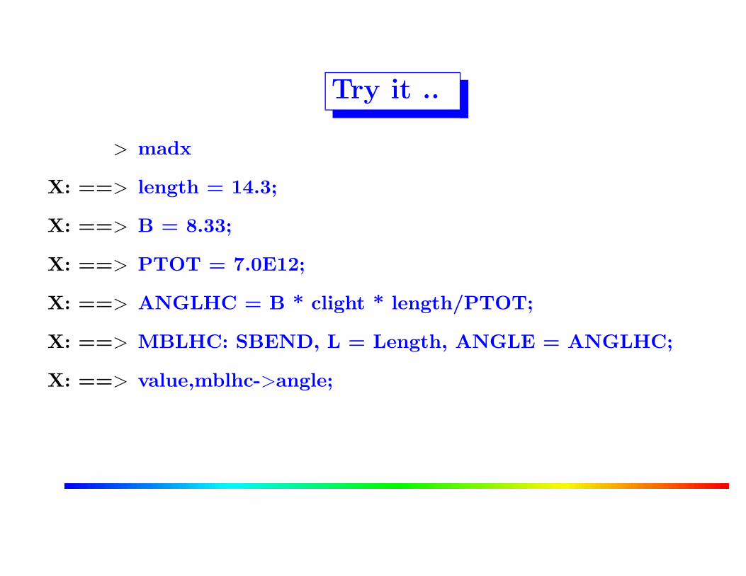
Try it ..
> madx
X: ==> length = 14.3;
X: ==> B = 8.33;
X: ==> PTOT = 7.0E12;
X: ==> ANGLHC = B * clight * length/PTOT;
X: ==> MBLHC: SBEND, L = Length, ANGLE = ANGLHC;
X: ==> value,mblhc->angle;

Thick and thin elements
Thick elements: so far all examples were thick
elements (or: lenses)
Specify length and strength separately (except
dipoles !)
+ More precise, path lengths and fringe fields
correct
- Not symplectic in tracking
- May need symplectic integration
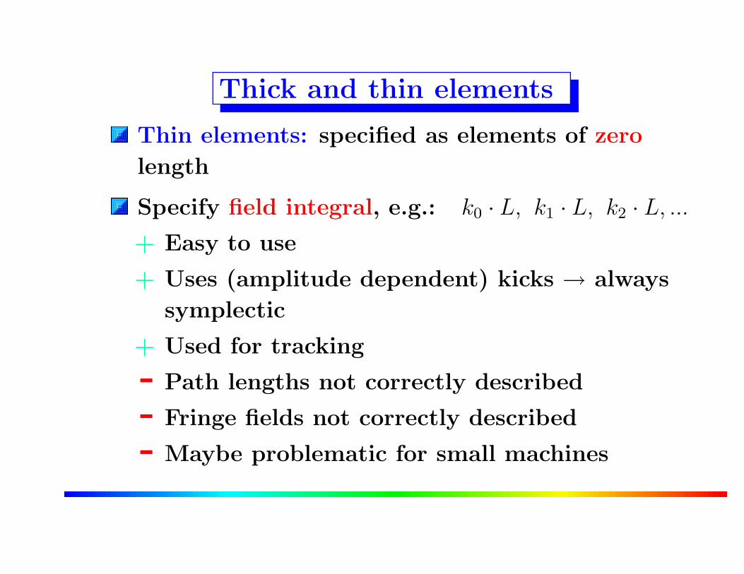
Thick and thin elements
Thin elements: specified as elements of zero
length
Specify field integral, e.g.: k0 · L, k1 · L, k2 · L, ...
+ Easy to use
+ Uses (amplitude dependent) kicks → always
symplectic
+ Used for tracking
- Path lengths not correctly described
- Fringe fields not correctly described
- Maybe problematic for small machines

Special MAD element: multipoles
Multipole: general element of zero length (thin lens), can
be used with one or more components of any order:
multip: multipole, knl := {kn0L, kn1L, kn2L, kn3L, ....};
→ knl = kn · L (normal components of nth order)
Very simple to use:
mul1: multipole, knl := {0,k1L,0,0,....};
is equivalent to definition of quadrupole (k1L =∫
1
p/cδBy
δx · dl)
mul0: multipole, knl = {angle,0,0,....};
is equivalent to definition of a bending magnet
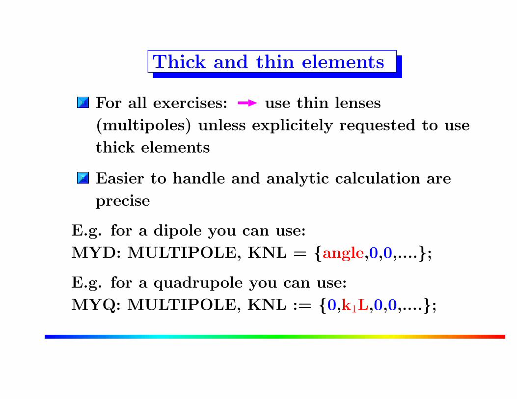
Thick and thin elements
For all exercises: use thin lenses
(multipoles) unless explicitely requested to use
thick elements
Easier to handle and analytic calculation are
precise
E.g. for a dipole you can use:
MYD: MULTIPOLE, KNL = {angle,0,0,....};
E.g. for a quadrupole you can use:
MYQ: MULTIPOLE, KNL := {0,k1L,0,0,....};

Definitions of sequence (position)
Have to assign position to the elements.
Positions are defined in a sequence with a name.
A position can be defined at CENTRE or EXIT or ENTRY
of an element .
Defined as absolute or relative position:
cassps: SEQUENCE, REFER=CENTRE, L=6912;
...
...
here specify position of all elements ...
...
...
ENDSEQUENCE;

Definitions of sequence (position)
cassps: SEQUENCE, refer=centre, l=6912;
...
...
MBL01: MBLA, at = 102.7484;
MBL02: MBLB, at = 112.7484;
MQ01: MQA, at = 119.3984;
BPM01: BPM, at = 1.75, from MQ01;
COR01: MCV01, at = LMCV/2 + LBPM/2, from BPM01;
MBL03: MBLA, at = 126.3484;
MBL04: MBLB, at = 136.3484;
MQ02: MQB, at = 142.9984;
BPM02: BPM, at = 1.75, from MQ02;
COR02: MCV02, at = LMCV/2 + LBPM/2, from BPM02;
...
...
ENDSEQUENCE;

Complete example: SPS (thick)
circum = 6912;
// bending magnets as thin lenses
mbsps: multipole,knl={0.007272205};
// quadrupoles and sextupoles
kqf = 0.0146315;
kqd = -0.0146434;
qfsps: quadrupole,l=3.085,k1 := kqf;
qdsps: quadrupole,l=3.085,k1 := kqd;
lsf: sextupole,l=1.0, k2 = 1.9518486E-02;
lsd: sextupole,l=1.0, k2 = -3.7618842E-02;
// monitors and orbit correctors
bpm: monitor,l=0.1;
ch: hkicker,l=0.1;
cv: vkicker,l=0.1;
cassps: sequence, l = circum;
start_machine: marker, at = 0;
qfsps, at = 1.5425;

lsf, at = 3.6425;
ch, at = 4.2425;
bpm, at = 4.3425;
mbsps, at = 5.0425;
mbsps, at = 11.4425;
mbsps, at = 23.6425;
mbsps, at = 30.0425;
qdsps, at = 33.5425;
lsd, at = 35.6425;
cv, at = 36.2425;
bpm, at = 36.3425;
....
....
qdsps, at = 6881.5425;
lsd, at = 6883.6425;
cv, at = 6884.2425;
bpm, at = 6884.3425;
mbsps, at = 6885.0425;
mbsps, at = 6891.4425;
mbsps, at = 6903.6425;
mbsps, at = 6910.0425;
end_machine: marker, at = 6912;
endsequence;
spsall.seq

circum=6912.0; // define the total length
ncell = 108; // define number of cells
lcell = circum/ncell;
// all magnets as multipoles
mbsps: multipole, knl={2.0*pi/(2*ncell)};
qfsps: multipole, knl={0.0, 4.36588E-02};
qdsps: multipole, knl={0.0,-4.36952E-02};
// sequence declaration;
cassps: sequence, refer=centre, l=circum;
n = 1;
while (n <= ncell) {
qfsps: qfsps, at=(n-1)*lcell;
mbsps: mbsps, at=(n-1)*lcell+16.0;
qdsps: qdsps, at=(n-1)*lcell+32.0;
mbsps: mbsps, at=(n-1)*lcell+48.0;
n = n + 1;
}
endsequence;
s1.seq

How to use MADX ?
Interactively:
– Type madx then input the commands on keyboard
(watch out for large machines !)
– Type madx then call input file(s):
call,file=sps.mad;
Batch mode:
– Type madx < sps.mad;
Our example (commands and machine description are
separated):
– sps.mad: MADX commands
– sps.seq: machine description
Simple MAD directives
Define the input
Define the beam
Initiate computations (Twiss calculation, error
assignment, orbit correction etc.)
Output results (tables, plotting)
Match desired parameters
Beware: may have default values !

Input definition and selection
Define the input:
call,”sps.seq”;
Selects a file with description of machine
Can be split into several files
Activate the machine:
USE, sequence=cassps;
Activates the sequence you want (described
in ”sps.seq”, which can contain more than
one)

We still need a beam !
Some computations need to know the type of
beam and its properties:
Particle type
Energy
Emittance, number of particles, intensity ....
BEAM, PARTICLE=name, MASS=mass, NPART=Nb,
CHARGE=q, ENERGY=E,.......;
Example:
BEAM, PARTICLE=proton, NPART=1.1E11, ENERGY=450,.......;

Initiate the computations
Execute an action (calculation of all lattice parameters
around the (circular !) machine):
twiss; or:
twiss, file=output; or:
twiss, sequence=cassps;
Execute an action (produce graphical output of
β-functions):
plot, haxis=s, vaxis=betx, bety;

Initiate the computations
Set parameters for an action with the SELECT
command (or defaults are used)
Calculation of Twiss parameters around the machine, store
selected lattice functions on file and plot β-functions:
select,flag=twiss,column=name,s,betx,bety;
twiss, sequence=cassps, file=twiss.out;
plot, haxis=s, vaxis=betx, bety, colour=100;

Initiate the computations
Calculation of Twiss parameters around the machine, store
and plot lattice functions for quadrupoles only:
select,flag=twiss,pattern=”ˆq.*”,column=name,s,betx,bety;
twiss, sequence=cassps, file=twiss.out;
plot, haxis=s, vaxis=betx, bety, colour=100;

Initiate the computations
Calculation of Twiss parameters around the machine, plot
between 10th and 16th quadrupoles only:
select,flag=twiss,pattern=”ˆq.*”,column=name,s,betx,bety;
twiss, sequence=cassps, file=twiss.out;
plot, haxis=s, vaxis=betx, bety, colour=100,
range=qd[10]/qd[16];

Initiate the computations
Make a geometrical survey of the machine layout, available
in a file:
select,flag=twiss,pattern=”ˆq.*”,column=name,s,betx,bety;
twiss, sequence=cassps, file=twiss.out;
plot, haxis=s, vaxis=betx, bety, colour=100,
range=qd[10]/qd[16];
survey, file=survey.cas;

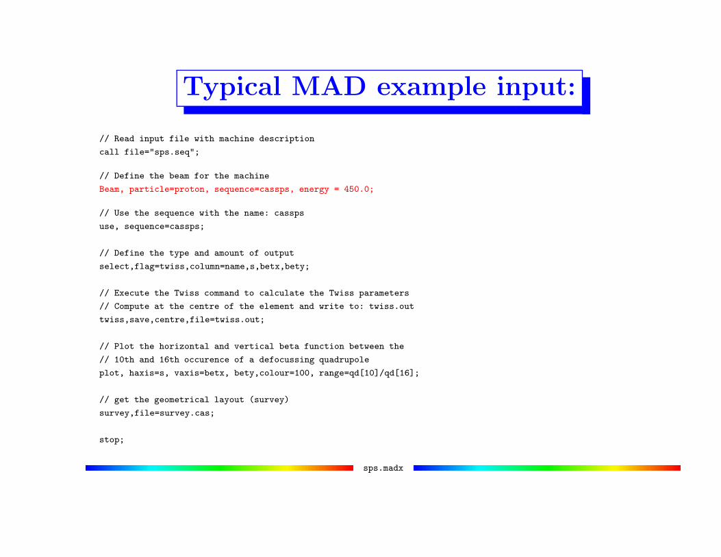
Typical MAD example input:
// Read input file with machine description
call file="sps.seq";
// Define the beam for the machine
Beam, particle=proton, sequence=cassps, energy=450.0;
// Use the sequence with the name: cassps
use, sequence=cassps;
// Define the type and amount of output
select,flag=twiss,column=name,s,betx,bety;
// Execute the Twiss command to calculate the Twiss parameters
// Compute at the centre of the element and write to: twiss.out
twiss,save,centre,file=twiss.out;
// Plot the horizontal and vertical beta function between the
// 10th and 16th occurence of a defocussing quadrupole
plot, haxis=s, vaxis=betx, bety,colour=100, range=qd[10]/qd[16];
// get the geometrical layout (survey)
survey,file=survey.cas;
stop;
sps.madx
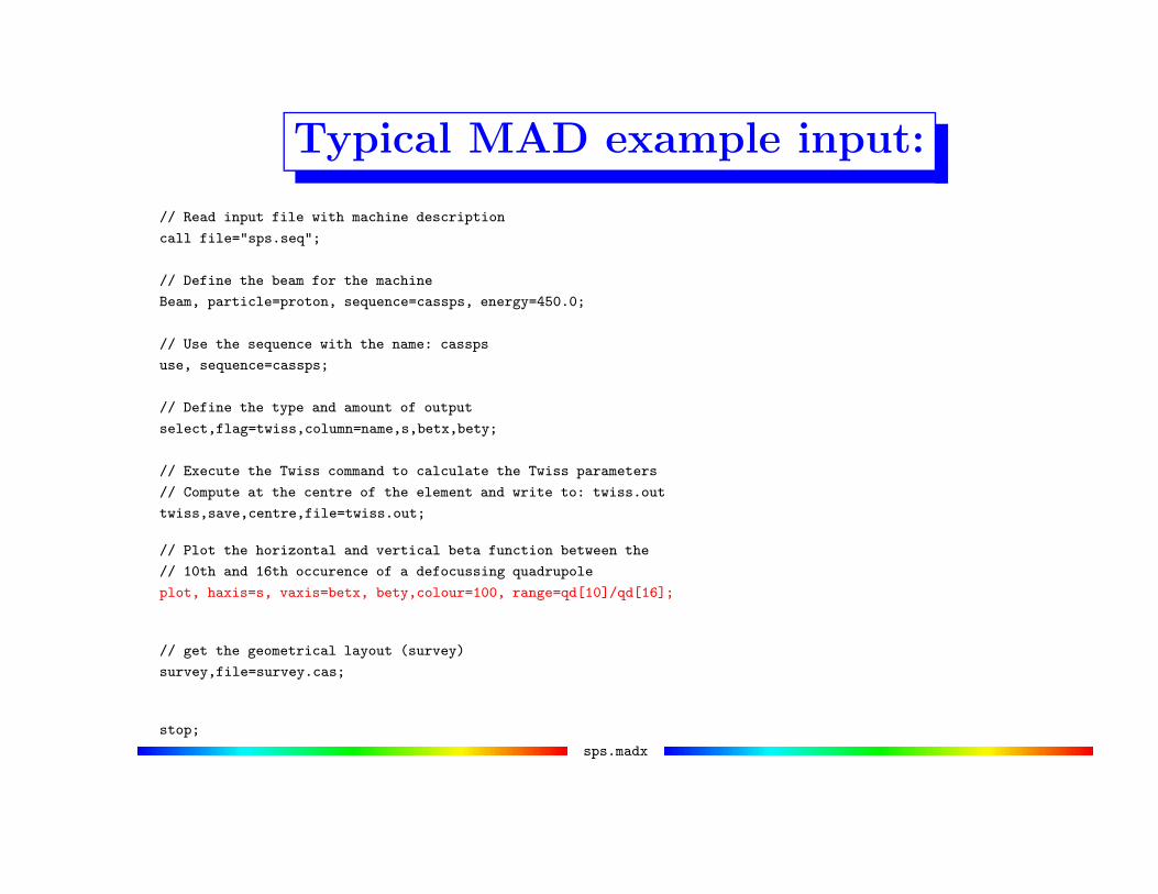
Typical MAD example input:
// Read input file with machine description
call file="sps.seq";
// Define the beam for the machine
Beam, particle=proton, sequence=cassps, energy = 450.0;
// Use the sequence with the name: cassps
use, sequence=cassps;
// Define the type and amount of output
select,flag=twiss,column=name,s,betx,bety;
// Execute the Twiss command to calculate the Twiss parameters
// Compute at the centre of the element and write to: twiss.out
twiss,save,centre,file=twiss.out;
// Plot the horizontal and vertical beta function between the
// 10th and 16th occurence of a defocussing quadrupole
plot, haxis=s, vaxis=betx, bety,colour=100, range=qd[10]/qd[16];
// get the geometrical layout (survey)
survey,file=survey.cas;
stop;
sps.madx

Typical MAD example input:
// Read input file with machine description
call file="sps.seq";
// Define the beam for the machine
Beam, particle=proton, sequence=cassps, energy=450.0;
// Use the sequence with the name: cassps
use, sequence=cassps;
// Define the type and amount of output
select,flag=twiss,column=name,s,betx,bety;
// Execute the Twiss command to calculate the Twiss parameters
// Compute at the centre of the element and write to: twiss.out
twiss,save,centre,file=twiss.out;
// Plot the horizontal and vertical beta function between the
// 10th and 16th occurence of a defocussing quadrupole
plot, haxis=s, vaxis=betx, bety,colour=100, range=qd[10]/qd[16];
// get the geometrical layout (survey)
survey,file=survey.cas;
stop;
sps.madx

Typical MAD example input:
// Read input file with machine description
call file="sps.seq";
// Define the beam for the machine
Beam, particle=proton, sequence=cassps, energy=450.0;
// Use the sequence with the name: cassps
use, sequence=cassps;
// Define the type and amount of output
select,flag=twiss,column=name,s,betx,bety;
// Execute the Twiss command to calculate the Twiss parameters
// Compute at the centre of the element and write to: twiss.out
twiss,save,centre,file=twiss.out;
// Plot the horizontal and vertical beta function between the
// 10th and 16th occurence of a defocussing quadrupole
plot, haxis=s, vaxis=betx, bety,colour=100, range=qd[10]/qd[16];
// get the geometrical layout (survey)
survey,file=survey.cas;
stop;
sps.madx

Typical MAD example input:
// Read input file with machine description
call file="sps.seq";
// Define the beam for the machine
Beam, particle=proton, sequence=cassps, energy=450.0;
// Use the sequence with the name: cassps
use, sequence=cassps;
// Define the type and amount of output
select,flag=twiss,column=name,s,betx,bety;
// Execute the Twiss command to calculate the Twiss parameters
// Compute at the centre of the element and write to: twiss.out
twiss,save,centre,file=twiss.out;
// Plot the horizontal and vertical beta function between the\\
// 10th and 16th occurence of a defocussing quadrupole\\
plot, haxis=s, vaxis=betx, bety,colour=100, range=qd[10]/qd[16];\\
// get the geometrical layout (survey)
survey,file=survey.cas;
stop;
sps.madx

Typical MAD output (summary):
++++++ table: summ
length orbit5 alfa gammatr
6912 -0 0.001667526597 24.4885807
q1 dq1 betxmax dxmax
26.57999204 -8.828683153e-09 108.7763569 2.575386926
dxrms xcomax xcorms q2
1.926988371 0 0 26.62004577
dq2 betymax dymax dyrms
4.9186549e-08 108.7331749 0 0
ycomax ycorms deltap synch_1
0 0 0 0

Typical MAD output (all elements):
* NAME S BETX BETY
$ %s %le %le %le
"CASSPS$START" 0 101.5961579 20.70328425
"START_MACHINE" 0 101.5961579 20.70328425
"DRIFT_0" 0.77125 105.1499566 19.94571028
"QF" 1.5425 108.7763569 19.26082066
"DRIFT_1" 2.5925 103.8571423 20.21112973
"LSF" 3.6425 99.07249356 21.29615787
"DRIFT_2" 3.9424975 97.73017837 21.6309074
"CH" 4.2425 96.39882586 21.97666007
"DRIFT_3" 4.2925 96.17800362 22.03535424
"BPM" 4.3425 95.95748651 22.0943539
"DRIFT_4" 4.6925025 94.4223997 22.51590816
"MBSPS" 5.0425 92.90228648 22.95242507
"DRIFT_5" 8.2425 79.69728195 27.63752778
"MBSPS" 11.4425 67.74212222 33.5738988
"DRIFT_6" 17.5425 48.41469349 48.35614376
"MBSPS" 23.6425 33.6289371 67.68523387
"DRIFT_5" 26.8425 27.68865546 79.6433337
"MBSPS" 30.0425 22.99821861 92.85270185
"DRIFT_7" 31.7925 20.96178735 100.6058286
"QD" 33.5425 19.29915001 108.7331749
"DRIFT_1" 34.5925 20.25187715 103.8118608
.......
.......
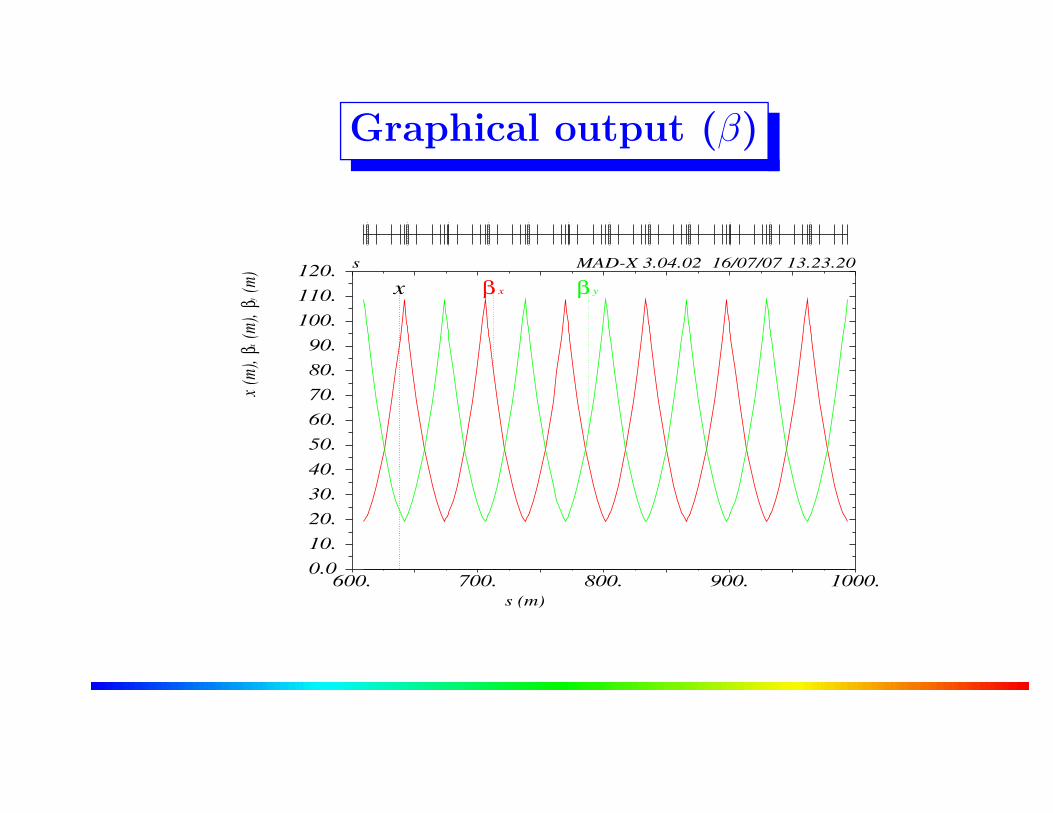
Graphical output (β)
600. 700. 800. 900. 1000. s (m)
s MAD-X 3.04.02 16/07/07 13.23.20
0.010.20.30.40.50.60.70.80.90.
100.110.120.
x(m)
,βx
(m),
βy(m
)
x β x β y
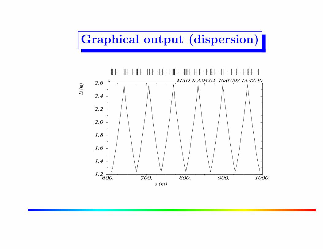
Graphical output (dispersion)
600. 700. 800. 900. 1000. s (m)
s MAD-X 3.04.02 16/07/07 13.42.40
1.2
1.4
1.6
1.8
2.0
2.2
2.4
2.6Dx
(m)

Graphical output (geometrical survey)
Output gives x, y, z, θ in absolute coordinates,
plotting x versus z should be a ring:
-2000
-1500
-1000
-500
0
500
1000
1500
2000
-3000 -2500 -2000 -1500 -1000 -500 0 500 1000
z (
m)
x (m)
Geometrical survey
-2000
-1500
-1000
-500
0
500
1000
1500
2000
-3000 -2500 -2000 -1500 -1000 -500 0 500 1000
z (
m)
x (m)
Geometrical survey

Optical matching
To get the optical configuration you want
compute settings yourself or use MAD for
matching
Main applications:
Setting global optical parameters
(e.g. tune, chromaticity)
Setting local optical parameters
(e.g. β-function, dispersion ..) part 2
Correction of imperfections part 2

Matching global parameters
Adjust strengths etc. to get desired properties
(e.g. tune, chromaticity)
Define the properties you want and the
elements to vary
Examples for global parameters (MAD
convention):
Q1, Q2:(horizontal and vertical tune)
dQ1, dQ2:(horizontal and vertical
chromaticity)

Matching global parameters
!Example, match horizontal (Q1) and vertical (Q2) tunes:
!Vary the quadrupole strengths kqf and kqd
!Quadrupoles must be defined with: ..., k1:=kqf, ... etc.
match, sequence=cassps;
global,sequence=cassps,Q1=26.58; → you want that !
global,sequence=cassps,Q2=26.62; → you want that !
vary,name=kqf, step=0.00001; → you vary that !
vary,name=kqd, step=0.00001; → you vary that !
Lmdif, calls=10, tolerance=1.0e-21; → (Method to use !)
endmatch;
spsmatch global.madx
(Some comments ... )
Input language seems heavy, but:
Can be interfaced to data base
Can be interfaced to other programs (e.g.
Mathematica)
Programs exist to generate the input
interactively
Allows web based applications
Allows to develop complex tools
MADX - part 2
We can:
Design and compute a regular lattice
Adjust basic machine parameters (tune,
chromaticity, β̂ ..)
What next:
Machines with imperfections and corrections
Design of dispersion suppressor
Design of low β insertion

Error assignment
MAD can assign errors to elements:
Alignment errors on all or selected elements
Field errors (up to high orders of multipole
fields) on all or selected elements
Errors are included in calculations (e.g. Twiss)
Correction algorithms can be applied
Error assignment
Can define alignment errors (EALIGN):
! assign error to all elements starting with Q
select,flag=error,pattern=”Q.*”;
Ealign, dx:=tgauss(3.0)*1.0e-4, dy:=tgauss(3.0)*2.0e-4;
Twiss,file=orbit.out; ! compute distorted machine
plot,haxis=s,vaxis=x,y; ! plot orbits in x and y
Can define field errors of any order (EFCOMP):
Remember the := !
See MADX Primer: page 14
sps orbit.madx

Orbit with alignment errors
0.0 2000. 4000. 6000. 8000.
s
−0.005
−0.004
−0.003
−0.002
−0.001
0.0
0.001
0.002
0.003
0.004
0.005x
x (m)
s (m)sps orbit.madx
How to measure an orbit ?
Needs Beam Position Monitors (keyword → MONITOR):
Gives position in one or both dimensions [ in m ]
BPMV: VMONITOR, L=0.1;
BPMV01: VMONITOR, L=0.1;
BPMV02: VMONITOR, L=0.1;
BPMV03: BPMV;
BPMH02: HMONITOR, L=0.1;
BPMHV01: MONITOR, L=0.1;
For orbit correction: consider orbit only at monitors ...
sps orbit.madx

How to correct an orbit ?
Needs Orbit corrector magnets (keyword →
HKICKER/VKICKER):
The strength of a corrector is an angle (kick) [ in rad ]
MCV: VKICKER, L=0.1;
MCV01: VKICKER, L=0.1, KICK := KCV01;
MCV02: VKICKER, L=0.1, KICK := KCV02;
MCV03: MCV, KICK := KCV03;
MCH02: HKICKER, L=0.1, KICK := KCH01;
Q: why do I use := ?
sps orbit.madx

Orbit correction algorithms in MADX
Best kick method (MICADO) in horizontal plane:
! Selected with MODE=MICADO
Correct,mode=MICADO,plane=x,
clist=”c.tab”,mlist=”m.tab”;
Singular Value Decomposition (SVD):
! Selected with MODE=SVD
Correct,mode=SVD,plane=x,
clist=”c.tab”,mlist=”m.tab”;
For details: see MADX Primer
sps orbit.madx
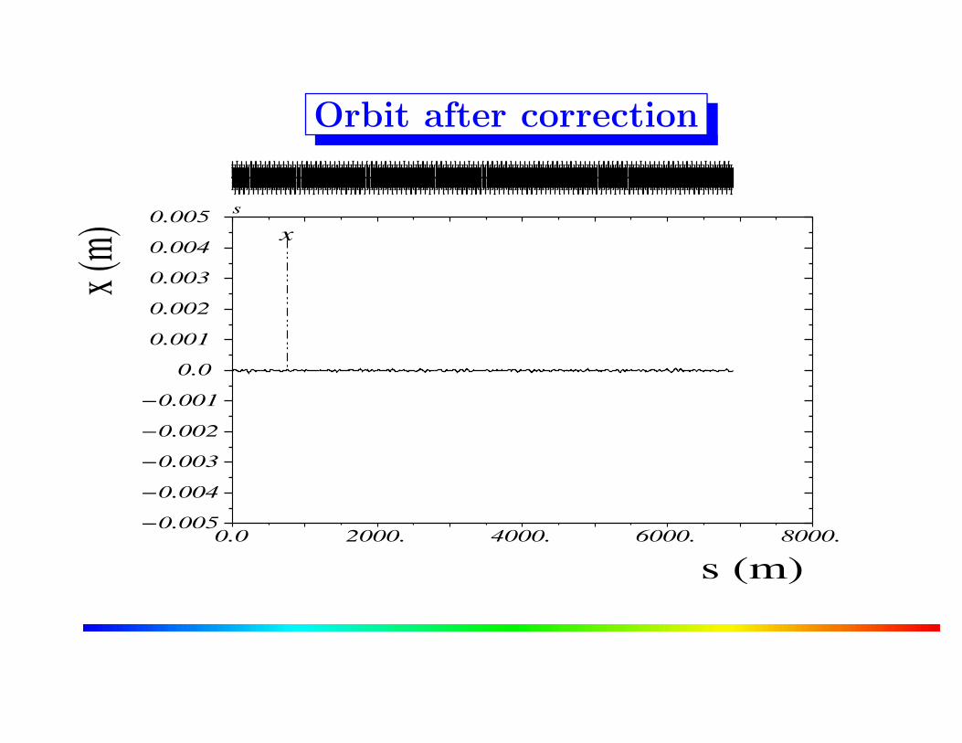
Orbit after correction
0.0 2000. 4000. 6000. 8000.
s
−0.005
−0.004
−0.003
−0.002
−0.001
0.0
0.001
0.002
0.003
0.004
0.005x
x (m)
s (m)

Optical matching
To get the optical configuration you want
matching
Main applications:
Setting global optical parameters (e.g. tune,
chromaticity)
Setting local optical parameters (e.g.
β-function, dispersion ..)
Correction of imperfections

Matching local parameters
Get local optical properties, but leave the rest
of the machine unchanged
Adjust strength of individual machine elements
Examples for local matching:
Low (or high) β insertions
Dispersion suppressors

Local optical matching
0
50
100
150
200
1000 1200 1400 1600 1800 2000

Local optical matching
0
50
100
150
200
250
1000 1200 1400 1600 1800 2000
beta bump.madx

Local optical matching
0
50
100
150
200
250
1000 1200 1400 1600 1800 2000
Don’t change this part !

Insertions (I)
How to add an insertion, e.g. two special cells ?
Start with periodic machine :
cassps: sequence, refer=centre, l=circum;
start_machine: marker, at = 0;
n = 1;
while (n <= ncell) {
qfsps: qfsps, at=(n-1)*lcell;
mbsps: mbsps, at=(n-1)*lcell+16.0;
qdsps: qdsps, at=(n-1)*lcell+32.00;
mbsps: mbsps, at=(n-1)*lcell+48.00;
n = n + 1; }
end_machine: marker at=circum;
endsequence;
Split it into several pieces
s1.seq

Local optical matching
0
50
100
150
200
1000 1200 1400 1600 1800 2000

Original lattice
� �� �� �� �� �� �
������
������
������
������
� �� �� �� �� �� �����
��
� �� �� �� �� �� �����
��
� �� �� �� �� �� �����
�� � �� �� �� �� �� �� �� �� �� �� �� �� �� �� �� �� �� �� �� �� �� �� �� �� �� �����
�������
��� �� �� �� �� �� �� �����
��� �� �� �� �� �� �� �� �� �� �� �� �� �
!!!!
!!
"""""""
######
$ $$ $$ $$ $$ $$ $$ $%%%%
%%& && && && && && && &' '' '' '' '' '' '
((((((
))))))
******
++++++
, ,, ,, ,, ,, ,, ,- -- -- -- -- -- -
......
//////
000000
111111
2 22 22 22 22 22 23333
33
4 44 44 44 44 44 45555
55 6 66 66 66 66 66 66 67 77 77 77 77 77 78 88 88 88 88 88 88 89 99 99 99 99 99 9::::
:::;;;;
;;
<<<<<<<
======
>>>>>>>
??????
@ @@ @@ @@ @@ @@ @@ @AAAA
AAB BB BB BB BB BB BB BC CC CC CC CC CC C
DDDDDD
EEEEEE F FF FF FF FF FF FF F
GGGGGG
H HH HH HH HH HH HH HI II II II II II I
JJJJJJ
KKKKKK
L LL LL LL LL LL LMMMM
MM
NNNNNN
OOOOOO
QDQD QDQF QFQF QF QF
QD QD QD QDQF QF QF QF
QD QD
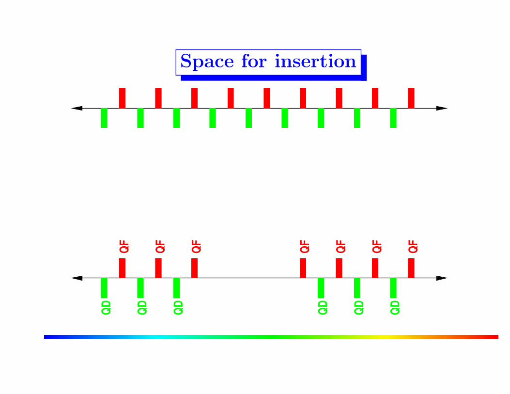
Space for insertion
P PP PP PP PP PP PQ QQ QQ QQ QQ QQ Q
RRRRRR
SSSSSS
TTTTTT
UUUUUU
VVVVVV
WWWWWW
X XX XX XX XX XX XYYYY
YY
Z ZZ ZZ ZZ ZZ ZZ Z[[[[
[[
\ \\ \\ \\ \\ \\ \]]]]
]] ^ ^^ ^^ ^^ ^^ ^^ ^^ ^_ __ __ __ __ __ _` `` `` `` `` `` `` `a aa aa aa aa aa abbbb
bbbcccc
ccd dd dd dd dd dd dd deeee
eef ff ff ff ff ff ff fg gg gg gg gg gg ghhhh
hhhiiii
ii
jjjjjjj
kkkkkk
l ll ll ll ll ll ll lmmmm
mmn nn nn nn nn nn nn no oo oo oo oo oo o
pppppp
qqqqqq
rrrrrr
ssssss
t tt tt tt tt tt tu uu uu uu uu uu u
vvvvvv
wwwwww
xxxxxx
yyyyyy
z zz zz zz zz zz z{{{{
{{
| || || || || || |}}}}
}} ~ ~~ ~~ ~~ ~~ ~~ ~~ ~� �� �� �� �� �� �� �� �� �� �� �� �� �� �� �� �� �� �� �����
�������
��
�������
������
�������
������
� �� �� �� �� �� �� �����
��� �� �� �� �� �� �� �� �� �� �� �� �� �
������
������
QD QD QD QD
QF QF QF QF QF QF QF
QD QD

Local optical matching
0
50
100
150
200
1000 1200 1400 1600 1800 2000

Adding quadrupoles
� �� �� �� �� �� �� �� �� �� �� �� �
������
������
������
������
������
������
� �� �� �� �� �� �����
��
� �� �� �� �� �� �����
��
� �� �� �� �� �� �����
�� � �� �� �� �� �� �� �� �� �� �� �� �� �� �� �� �� �� �� �� �� �� �� �� �� �� �
¡¡¡¡
¡¡¢ ¢¢ ¢¢ ¢¢ ¢¢ ¢¢ ¢¢ ¢££££
££¤ ¤¤ ¤¤ ¤¤ ¤¤ ¤¤ ¤¤ ¤¥ ¥¥ ¥¥ ¥¥ ¥¥ ¥¥ ¥¦¦¦¦
¦¦¦§§§§
§§
¨¨¨¨¨¨¨
©©©©©©
ª ªª ªª ªª ªª ªª ªª ª««««
««¬ ¬¬ ¬¬ ¬¬ ¬¬ ¬¬ ¬¬ ¬
®®®®®®
¯¯¯¯¯¯
°°°°°°
±±±±±±
² ²² ²² ²² ²² ²² ²³ ³³ ³³ ³³ ³³ ³³ ³
´´´´´´
µµµµµµ
¶¶¶¶¶¶
······
¸ ¸¸ ¸¸ ¸¸ ¸¸ ¸¸ ¸¹¹¹¹
¹¹
º ºº ºº ºº ºº ºº º»»»»
»» ¼ ¼¼ ¼¼ ¼¼ ¼¼ ¼¼ ¼¼ ¼½ ½½ ½½ ½½ ½½ ½½ ½¾ ¾¾ ¾¾ ¾¾ ¾¾ ¾¾ ¾¾ ¾¿ ¿¿ ¿¿ ¿¿ ¿¿ ¿¿ ¿ÀÀÀÀ
ÀÀÀÁÁÁÁ
ÁÁ
ÂÂÂÂÂÂÂ
ÃÃÃÃÃÃ
ÄÄÄÄÄÄÄ
ÅÅÅÅÅÅ
Æ ÆÆ ÆÆ ÆÆ ÆÆ ÆÆ ÆÆ ÆÇÇÇÇ
ÇÇÈ ÈÈ ÈÈ ÈÈ ÈÈ ÈÈ ÈÈ ÈÉ ÉÉ ÉÉ ÉÉ ÉÉ ÉÉ É
ÊÊÊÊÊÊ
ËËËËËË
ÌÌÌÌÌÌ
ÍÍÍÍÍÍ Î ÎÎ ÎÎ ÎÎ ÎÎ ÎÎ ÎÎ Î
ÏÏÏÏÏÏ
Ð ÐÐ ÐÐ ÐÐ ÐÐ ÐÐ ÐÑÑÑÑ
ÑÑ Ò ÒÒ ÒÒ ÒÒ ÒÒ ÒÒ ÒÒ ÒÓ ÓÓ ÓÓ ÓÓ ÓÓ ÓÓ Ó
ÔÔÔÔÔÔ
ÕÕÕÕÕÕ
Q1 Q3Q4
Q5
Q2
QD QD QD QD
QF QF QF QF

Insertions (II)
Split it into several pieces
cassps: sequence, refer=centre, l=circum;
n = 1;
while (n ≤ ncell-2) {
qfsps: qfsps, at=(n-1)*lcell;
mbsps: mbsps, at=(n-1)*lcell+16.0;
qdsps: qdsps, at=(n-1)*lcell+32.00;
mbsps: mbsps, at=(n-1)*lcell+48.00;
n = n + 1;
}
qf1 : qf1 , at=(ncell-2)*lcell;
mbsps: mbsps, at=(ncell-2)*lcell+16.0;
qd1 : qd1 , at=(ncell-2)*lcell+32.00;
mbsps: mbsps, at=(ncell-2)*lcell+48.00;
qf2 : qf2 , at=(ncell-1)*lcell;
mbsps: mbsps, at=(ncell-1)*lcell+16.0;
qd2 : qd2 , at=(ncell-1)*lcell+32.00;
mbsps: mbsps, at=(ncell-1)*lcell+48.00;
endsequence;
s1 ins.seq

Inserting sequences
Sequences can be (re-)used like elements:
cascell1: sequence, refer=centre, l=lcell;
qfsps: qfsps, at=0.0;
mbsps: mbsps, at=0.25*lcell;
qdsps: qdsps, at=0.50*lcell;
mbsps: mbsps, at=0.75*lcell;
endsequence;
allcells: sequence, refer=centre, l=ncell*lcell;
n = 1;
while (n < ncell+1) {
cascell1, at=(n-1)*lcell;
n = n + 1;
}
endsequence;
seqinseq.seq

Local optical matching
0
50
100
150
200
1000 1200 1400 1600 1800 2000
xx

Matching techniques I(a)
Use of markers:
→ Have no effect on the optics
→ Used to mark a position in the machine
→ Can be used as reference in matching etc.
Use:
left: MARKER, at=position;
right: MARKER, at=position;
Matching techniques I(b)
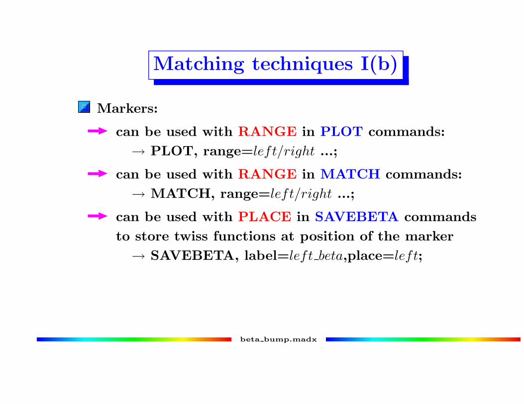
Markers:
can be used with RANGE in PLOT commands:
→ PLOT, range=left/right ...;
can be used with RANGE in MATCH commands:
→ MATCH, range=left/right ...;
can be used with PLACE in SAVEBETA commands
to store twiss functions at position of the marker
→ SAVEBETA, label=left beta,place=left;
beta bump.madx

Use of MARKERS
Ö ÖÖ ÖÖ ÖÖ ÖÖ ÖÖ Ö× ×× ×× ×× ×× ×× ×
ØØØØØØ
ÙÙÙÙÙÙ
ÚÚÚÚÚÚ
ÛÛÛÛÛÛ
ÜÜÜÜÜÜ
ÝÝÝÝÝÝ
Þ ÞÞ ÞÞ ÞÞ ÞÞ ÞÞ Þßßßß
ßß
à àà àà àà àà àà àáááá
áá
â ââ ââ ââ ââ ââ âãããã
ãã ä ää ää ää ää ää ää äå åå åå åå åå åå åå åæ ææ ææ ææ ææ ææ ææ æç çç çç çç çç çç çç çèèèè
èèèéééé
éééê êê êê êê êê êê êê êëëëë
ëëëì ìì ìì ìì ìì ìì ìì ìí íí íí íí íí íí íí íîîîî
îîîïïïï
ïïï
ððððððð
ñññññññ
ò òò òò òò òò òò òò òóóóó
óóóô ôô ôô ôô ôô ôô ôô ôõ õõ õõ õõ õõ õõ õõ õ
öööööö
÷÷÷÷÷÷
øøøøøø
ùùùùùù
ú úú úú úú úú úú úû ûû ûû ûû ûû ûû û
üüüüüü
ýýýýýý
þþþþþþ
ÿÿÿÿÿÿ
� �� �� �� �� �� �
������
� �� �� �� �� �� �
������ � �� �� �
� �� �� �� �� �� �� �� �� �� �� �
� �� �� �� �� �� �� �
� �� �� �� �� �� �� �
�������
�������
�������
� �� �� �� �� �� �� �
�������
� �� �� �� �� �� �� �
� �� �� �� �� �� �� �
������
������ � �� �� �� �
� �� �� �����
���� �� �� �� �
� �� �� �� �� �� �� �
� �� �� �
������
������
� �� �� �� �� �� �
������
������
������
QDQD QDQF QFQF QF QF
QD QD QD QDQF QF QF QF
QD QD

Use of MARKERS
� �� �� �� �� �� �
� �� �� �� �� �� �
!!!!!!
""""""
######
$$$$$$
%%%%%%
& && && && && && &
''''''
( (( (( (( (( (( (
))))))
* ** ** ** ** ** *
++++++ , ,, ,, ,
, ,, ,, ,, ,- -- -- -- -- -- -- -
. .. .. .. .. .. .. .
/ // // // // // // /
0000000
1111111
2 22 22 22 22 22 22 2
3333333
4 44 44 44 44 44 44 4
5 55 55 55 55 55 55 5
6666666
7777777
8888888
9999999
: :: :: :: :: :: :: :
;;;;;;;
< << << << << << << <
= == == == == == == =
>>>>>>
??????
@@@@@@
AAAAAA
B BB BB BB BB BB B
C CC CC CC CC CC C
DDDDDD
EEEEEE
FFFFFF
GGGGGG
H HH HH HH HH HH H
IIIIII
J JJ JJ JJ JJ JJ J
KKKKKK L LL LL L
L LL LL LL LM MM MM MM MM MM MM M
N NN NN NN NN NN NN N
O OO OO OO OO OO OO O
PPPPPPP
QQQQQQQ
RRRRRRR
SSSSSSS
TTTTTTT
UUUUUUU
V VV VV VV VV VV VV V
WWWWWWW
X XX XX XX XX XX XX X
Y YY YY YY YY YY YY Y
ZZZZZZ
[[[[[[
\\\\\\
]]]]]] ^ ^^ ^^ ^
^ ^^ ^^ ^^ ^_______
` `` `` `` `` `` `
aaaaaa b bb bb bb b
b bb bb bc cc cc cc c
c cc cc cdddd
ddeeee
eeQ1 Q3
Q4Q5
Q2
QD QD QD QD
QF QF QF QF

Use of MARKERS
f ff ff ff ff ff f
g gg gg gg gg gg g
hhhhhh
iiiiii
jjjjjj
kkkkkk
llllll
mmmmmm
n nn nn nn nn nn n
oooooo
p pp pp pp pp pp p
qqqqqq
r rr rr rr rr rr r
ssssss t tt tt t
t tt tt tt tu uu uu uu uu uu uu u
v vv vv vv vv vv vv v
w ww ww ww ww ww ww w
xxxxxxx
yyyyyyy
z zz zz zz zz zz zz z
{{{{{{{
| || || || || || || |
} }} }} }} }} }} }} }
~~~~~~~
�������
�������
�������
� �� �� �� �� �� �� �
�������
� �� �� �� �� �� �� �
� �� �� �� �� �� �� �
������
������
������
������
� �� �� �� �� �� �
� �� �� �� �� �� �
������
������
������
������
� �� �� �� �� �� �
������
� �� �� �� �� �� �
������ � �� �� �
� �� �� �� �� �� �� �� �� �� �� �
� �� �� �� �� �� �� �
� �� �� �� �� �� �� �
�������
�������
�������
�������
�������
�������
� �� �� �� �� �� �� �
�������
¡ ¡¡ ¡¡ ¡¡ ¡¡ ¡¡ ¡¡ ¡
¢¢¢¢¢¢
££££££
¤¤¤¤¤¤
¥¥¥¥¥¥ ¦ ¦¦ ¦¦ ¦
¦ ¦¦ ¦¦ ¦¦ ¦§§§§§§§
¨ ¨¨ ¨¨ ¨¨ ¨¨ ¨¨ ¨
©©©©©© ª ªª ªª ªª ª
ª ªª ªª ª« «« «« «« «
« «« «« «¬¬¬¬
¬¬
left
Q1 Q3Q4
Q5
Q2
right
Use of MARKERS
® ®® ®® ®® ®® ®® ®
¯ ¯¯ ¯¯ ¯¯ ¯¯ ¯¯ ¯
°°°°°°
±±±±±±
²²²²²²
³³³³³³
´´´´´´
µµµµµµ
¶ ¶¶ ¶¶ ¶¶ ¶¶ ¶¶ ¶
······
¸ ¸¸ ¸¸ ¸¸ ¸¸ ¸¸ ¸
¹¹¹¹¹¹
º ºº ºº ºº ºº ºº º
»»»»»» ¼ ¼¼ ¼¼ ¼
¼ ¼¼ ¼¼ ¼¼ ¼½ ½½ ½½ ½½ ½½ ½½ ½½ ½
¾ ¾¾ ¾¾ ¾¾ ¾¾ ¾¾ ¾¾ ¾
¿ ¿¿ ¿¿ ¿¿ ¿¿ ¿¿ ¿¿ ¿
ÀÀÀÀÀÀÀ
ÁÁÁÁÁÁÁ
 Â Â Â Â Â Â Â
ÃÃÃÃÃÃÃ
Ä ÄÄ ÄÄ ÄÄ ÄÄ ÄÄ ÄÄ Ä
Å ÅÅ ÅÅ ÅÅ ÅÅ ÅÅ ÅÅ Å
ÆÆÆÆÆÆÆ
ÇÇÇÇÇÇÇ
ÈÈÈÈÈÈÈ
ÉÉÉÉÉÉÉ
Ê ÊÊ ÊÊ ÊÊ ÊÊ ÊÊ ÊÊ Ê
ËËËËËËË
Ì ÌÌ ÌÌ ÌÌ ÌÌ ÌÌ ÌÌ Ì
Í ÍÍ ÍÍ ÍÍ ÍÍ ÍÍ ÍÍ Í
ÎÎÎÎÎÎ
ÏÏÏÏÏÏ
ÐÐÐÐÐÐ
ÑÑÑÑÑÑ
Ò ÒÒ ÒÒ ÒÒ ÒÒ ÒÒ Ò
Ó ÓÓ ÓÓ ÓÓ ÓÓ ÓÓ Ó
ÔÔÔÔÔÔ
ÕÕÕÕÕÕ
ÖÖÖÖÖÖ
××××××
Ø ØØ ØØ ØØ ØØ ØØ Ø
ÙÙÙÙÙÙ
Ú ÚÚ ÚÚ ÚÚ ÚÚ ÚÚ Ú
ÛÛÛÛÛÛ Ü ÜÜ ÜÜ Ü
Ü ÜÜ ÜÜ ÜÜ ÜÝ ÝÝ ÝÝ ÝÝ ÝÝ ÝÝ ÝÝ Ý
Þ ÞÞ ÞÞ ÞÞ ÞÞ ÞÞ ÞÞ Þ
ß ßß ßß ßß ßß ßß ßß ß
ààààààà
ááááááá
âââââââ
ããããããã
äääääää
ååååååå
æ ææ ææ ææ ææ ææ ææ æ
ççççççç
è èè èè èè èè èè èè è
é éé éé éé éé éé éé é
êêêêêê
ëëëëëë
ìììììì
íííííí î îî îî î
î îî îî îî îïïïïïïï
ð ðð ðð ðð ðð ðð ð
ññññññ ò òò òò òò ò
ò òò òò òó óó óó óó ó
ó óó óó óôôôô
ôôõõõõ
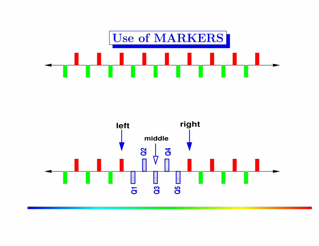
õõleft
Q1 Q3Q4
Q5
Q2middle
right
Matching techniques II
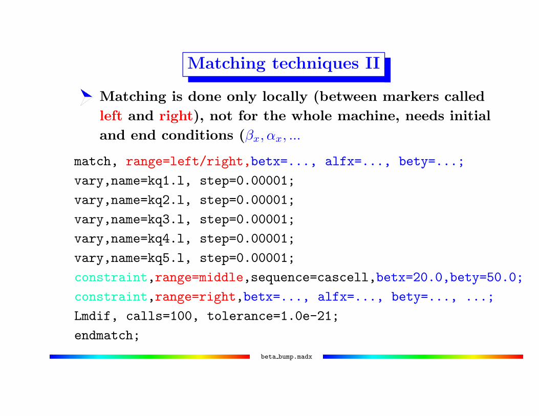
ö ö ö ö ö ö ö ö ö ö ö ö ö ö öö ö ö ö ö ö ö ö ö ö ö ö ö ö öö ö ö ö ö ö ö ö ö ö ö ö ö ö öö ö ö ö ö ö ö ö ö ö ö ö ö ö öö ö ö ö ö ö ö ö ö ö ö ö ö ö öö ö ö ö ö ö ö ö ö ö ö ö ö ö öö ö ö ö ö ö ö ö ö ö ö ö ö ö öö ö ö ö ö ö ö ö ö ö ö ö ö ö öö ö ö ö ö ö ö ö ö ö ö ö ö ö öö ö ö ö ö ö ö ö ö ö ö ö ö ö öö ö ö ö ö ö ö ö ö ö ö ö ö ö öö ö ö ö ö ö ö ö ö ö ö ö ö ö öö ö ö ö ö ö ö ö ö ö ö ö ö ö öö ö ö ö ö ö ö ö ö ö ö ö ö ö öö ö ö ö ö ö ö ö ö ö ö ö ö ö öö ö ö ö ö ö ö ö ö ö ö ö ö ö öö ö ö ö ö ö ö ö ö ö ö ö ö ö öö ö ö ö ö ö ö ö ö ö ö ö ö ö öö ö ö ö ö ö ö ö ö ö ö ö ö ö öö ö ö ö ö ö ö ö ö ö ö ö ö ö öø÷ ÷ ÷ ÷ ÷ ÷ ÷ ÷ ÷ ÷ ÷ ÷ ÷ ÷ ÷÷ ÷ ÷ ÷ ÷ ÷ ÷ ÷ ÷ ÷ ÷ ÷ ÷ ÷ ÷÷ ÷ ÷ ÷ ÷ ÷ ÷ ÷ ÷ ÷ ÷ ÷ ÷ ÷ ÷÷ ÷ ÷ ÷ ÷ ÷ ÷ ÷ ÷ ÷ ÷ ÷ ÷ ÷ ÷÷ ÷ ÷ ÷ ÷ ÷ ÷ ÷ ÷ ÷ ÷ ÷ ÷ ÷ ÷÷ ÷ ÷ ÷ ÷ ÷ ÷ ÷ ÷ ÷ ÷ ÷ ÷ ÷ ÷÷ ÷ ÷ ÷ ÷ ÷ ÷ ÷ ÷ ÷ ÷ ÷ ÷ ÷ ÷÷ ÷ ÷ ÷ ÷ ÷ ÷ ÷ ÷ ÷ ÷ ÷ ÷ ÷ ÷÷ ÷ ÷ ÷ ÷ ÷ ÷ ÷ ÷ ÷ ÷ ÷ ÷ ÷ ÷÷ ÷ ÷ ÷ ÷ ÷ ÷ ÷ ÷ ÷ ÷ ÷ ÷ ÷ ÷÷ ÷ ÷ ÷ ÷ ÷ ÷ ÷ ÷ ÷ ÷ ÷ ÷ ÷ ÷÷ ÷ ÷ ÷ ÷ ÷ ÷ ÷ ÷ ÷ ÷ ÷ ÷ ÷ ÷÷ ÷ ÷ ÷ ÷ ÷ ÷ ÷ ÷ ÷ ÷ ÷ ÷ ÷ ÷÷ ÷ ÷ ÷ ÷ ÷ ÷ ÷ ÷ ÷ ÷ ÷ ÷ ÷ ÷÷ ÷ ÷ ÷ ÷ ÷ ÷ ÷ ÷ ÷ ÷ ÷ ÷ ÷ ÷÷ ÷ ÷ ÷ ÷ ÷ ÷ ÷ ÷ ÷ ÷ ÷ ÷ ÷ ÷÷ ÷ ÷ ÷ ÷ ÷ ÷ ÷ ÷ ÷ ÷ ÷ ÷ ÷ ÷÷ ÷ ÷ ÷ ÷ ÷ ÷ ÷ ÷ ÷ ÷ ÷ ÷ ÷ ÷÷ ÷ ÷ ÷ ÷ ÷ ÷ ÷ ÷ ÷ ÷ ÷ ÷ ÷ ÷÷ ÷ ÷ ÷ ÷ ÷ ÷ ÷ ÷ ÷ ÷ ÷ ÷ ÷ ÷Matching is done only locally (between markers called
left and right), not for the whole machine, needs initial
and end conditions (βx, αx, ...
match, range=left/right,betx=..., alfx=..., bety=...;
vary,name=kq1.l, step=0.00001;
vary,name=kq2.l, step=0.00001;
vary,name=kq3.l, step=0.00001;
vary,name=kq4.l, step=0.00001;
vary,name=kq5.l, step=0.00001;
constraint,range=middle,sequence=cascell,betx=20.0,bety=50.0;
constraint,range=right,betx=..., alfx=..., bety=..., ...;
Lmdif, calls=100, tolerance=1.0e-21;
endmatch;
beta bump.madx

Using SAVEBETA to store optical functions
savebeta,label=tw left,place=left;
savebeta,label=tw right,place=right;
twiss;
match, sequence=cascell,range=left/right,beta0=tw left;
vary,name=kq1.l, step=0.00001;
vary,name=kq2.l, step=0.00001;
vary,name=kq3.l, step=0.00001;
vary,name=kq4.l, step=0.00001;
vary,name=kq5.l, step=0.00001;
constraint,range=middle,sequence=cascell,betx=20.0,bety=50.0;
constraint,range=right,sequence=cascell,beta0=tw right;
Lmdif, calls=100, tolerance=1.0e-21;
endmatch;beta bump.madx

Matching techniques IV
ù ù ù ù ù ù ù ù ù ù ù ù ù ù ùù ù ù ù ù ù ù ù ù ù ù ù ù ù ùù ù ù ù ù ù ù ù ù ù ù ù ù ù ùù ù ù ù ù ù ù ù ù ù ù ù ù ù ùù ù ù ù ù ù ù ù ù ù ù ù ù ù ùù ù ù ù ù ù ù ù ù ù ù ù ù ù ùù ù ù ù ù ù ù ù ù ù ù ù ù ù ùù ù ù ù ù ù ù ù ù ù ù ù ù ù ùù ù ù ù ù ù ù ù ù ù ù ù ù ù ùù ù ù ù ù ù ù ù ù ù ù ù ù ù ùù ù ù ù ù ù ù ù ù ù ù ù ù ù ùù ù ù ù ù ù ù ù ù ù ù ù ù ù ùù ù ù ù ù ù ù ù ù ù ù ù ù ù ùù ù ù ù ù ù ù ù ù ù ù ù ù ù ùù ù ù ù ù ù ù ù ù ù ù ù ù ù ùù ù ù ù ù ù ù ù ù ù ù ù ù ù ùù ù ù ù ù ù ù ù ù ù ù ù ù ù ùù ù ù ù ù ù ù ù ù ù ù ù ù ù ùù ù ù ù ù ù ù ù ù ù ù ù ù ù ùù ù ù ù ù ù ù ù ù ù ù ù ù ù ùøú ú ú ú ú ú ú ú ú ú ú ú ú ú úú ú ú ú ú ú ú ú ú ú ú ú ú ú úú ú ú ú ú ú ú ú ú ú ú ú ú ú úú ú ú ú ú ú ú ú ú ú ú ú ú ú úú ú ú ú ú ú ú ú ú ú ú ú ú ú úú ú ú ú ú ú ú ú ú ú ú ú ú ú úú ú ú ú ú ú ú ú ú ú ú ú ú ú úú ú ú ú ú ú ú ú ú ú ú ú ú ú úú ú ú ú ú ú ú ú ú ú ú ú ú ú úú ú ú ú ú ú ú ú ú ú ú ú ú ú úú ú ú ú ú ú ú ú ú ú ú ú ú ú úú ú ú ú ú ú ú ú ú ú ú ú ú ú úú ú ú ú ú ú ú ú ú ú ú ú ú ú úú ú ú ú ú ú ú ú ú ú ú ú ú ú úú ú ú ú ú ú ú ú ú ú ú ú ú ú úú ú ú ú ú ú ú ú ú ú ú ú ú ú úú ú ú ú ú ú ú ú ú ú ú ú ú ú úú ú ú ú ú ú ú ú ú ú ú ú ú ú úú ú ú ú ú ú ú ú ú ú ú ú ú ú úú ú ú ú ú ú ú ú ú ú ú ú ú ú úConstraints on all quadrupoles, using SAVEBETA:
savebeta,label=qf,place=quadf_marker:
twiss;
match, sequence=cascell;
vary,name=kqf, step=0.00001;
vary,name=kqd, step=0.00001;
constraint,pattern="^qf.*",sequence=cascell,betx=qf->betax,
bety=qf->betay;
constraint,pattern="^qd.*",sequence=cascell,betx=qf->betay,
bety=qf->betax;
Lmdif, calls=100, tolerance=1.0e-21;
endmatch;
Matching techniques V
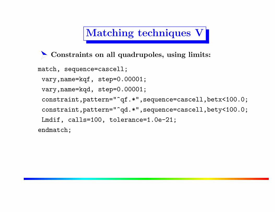
û û û û û û û û û û û û û û ûû û û û û û û û û û û û û û ûû û û û û û û û û û û û û û ûû û û û û û û û û û û û û û ûû û û û û û û û û û û û û û ûû û û û û û û û û û û û û û ûû û û û û û û û û û û û û û ûû û û û û û û û û û û û û û ûû û û û û û û û û û û û û û ûû û û û û û û û û û û û û û ûû û û û û û û û û û û û û û ûû û û û û û û û û û û û û û ûû û û û û û û û û û û û û û ûû û û û û û û û û û û û û û ûû û û û û û û û û û û û û û ûû û û û û û û û û û û û û û ûû û û û û û û û û û û û û û ûû û û û û û û û û û û û û û ûû û û û û û û û û û û û û û ûû û û û û û û û û û û û û û ûøü ü ü ü ü ü ü ü ü ü ü ü ü ü üü ü ü ü ü ü ü ü ü ü ü ü ü ü üü ü ü ü ü ü ü ü ü ü ü ü ü ü üü ü ü ü ü ü ü ü ü ü ü ü ü ü üü ü ü ü ü ü ü ü ü ü ü ü ü ü üü ü ü ü ü ü ü ü ü ü ü ü ü ü üü ü ü ü ü ü ü ü ü ü ü ü ü ü üü ü ü ü ü ü ü ü ü ü ü ü ü ü üü ü ü ü ü ü ü ü ü ü ü ü ü ü üü ü ü ü ü ü ü ü ü ü ü ü ü ü üü ü ü ü ü ü ü ü ü ü ü ü ü ü üü ü ü ü ü ü ü ü ü ü ü ü ü ü üü ü ü ü ü ü ü ü ü ü ü ü ü ü üü ü ü ü ü ü ü ü ü ü ü ü ü ü üü ü ü ü ü ü ü ü ü ü ü ü ü ü üü ü ü ü ü ü ü ü ü ü ü ü ü ü üü ü ü ü ü ü ü ü ü ü ü ü ü ü üü ü ü ü ü ü ü ü ü ü ü ü ü ü üü ü ü ü ü ü ü ü ü ü ü ü ü ü üü ü ü ü ü ü ü ü ü ü ü ü ü ü üConstraints on all quadrupoles, using limits:
match, sequence=cascell;
vary,name=kqf, step=0.00001;
vary,name=kqd, step=0.00001;
constraint,pattern="^qf.*",sequence=cascell,betx<100.0;
constraint,pattern="^qd.*",sequence=cascell,bety<100.0;
Lmdif, calls=100, tolerance=1.0e-21;
endmatch;

Particle tracking
ý ý ý ý ý ý ý ý ý ý ý ý ý ý ýý ý ý ý ý ý ý ý ý ý ý ý ý ý ýý ý ý ý ý ý ý ý ý ý ý ý ý ý ýý ý ý ý ý ý ý ý ý ý ý ý ý ý ýý ý ý ý ý ý ý ý ý ý ý ý ý ý ýý ý ý ý ý ý ý ý ý ý ý ý ý ý ýý ý ý ý ý ý ý ý ý ý ý ý ý ý ýý ý ý ý ý ý ý ý ý ý ý ý ý ý ýý ý ý ý ý ý ý ý ý ý ý ý ý ý ýý ý ý ý ý ý ý ý ý ý ý ý ý ý ýý ý ý ý ý ý ý ý ý ý ý ý ý ý ýý ý ý ý ý ý ý ý ý ý ý ý ý ý ýý ý ý ý ý ý ý ý ý ý ý ý ý ý ýý ý ý ý ý ý ý ý ý ý ý ý ý ý ýý ý ý ý ý ý ý ý ý ý ý ý ý ý ýý ý ý ý ý ý ý ý ý ý ý ý ý ý ýý ý ý ý ý ý ý ý ý ý ý ý ý ý ýý ý ý ý ý ý ý ý ý ý ý ý ý ý ýý ý ý ý ý ý ý ý ý ý ý ý ý ý ýý ý ý ý ý ý ý ý ý ý ý ý ý ý ýøþ þ þ þ þ þ þ þ þ þ þ þ þ þ þþ þ þ þ þ þ þ þ þ þ þ þ þ þ þþ þ þ þ þ þ þ þ þ þ þ þ þ þ þþ þ þ þ þ þ þ þ þ þ þ þ þ þ þþ þ þ þ þ þ þ þ þ þ þ þ þ þ þþ þ þ þ þ þ þ þ þ þ þ þ þ þ þþ þ þ þ þ þ þ þ þ þ þ þ þ þ þþ þ þ þ þ þ þ þ þ þ þ þ þ þ þþ þ þ þ þ þ þ þ þ þ þ þ þ þ þþ þ þ þ þ þ þ þ þ þ þ þ þ þ þþ þ þ þ þ þ þ þ þ þ þ þ þ þ þþ þ þ þ þ þ þ þ þ þ þ þ þ þ þþ þ þ þ þ þ þ þ þ þ þ þ þ þ þþ þ þ þ þ þ þ þ þ þ þ þ þ þ þþ þ þ þ þ þ þ þ þ þ þ þ þ þ þþ þ þ þ þ þ þ þ þ þ þ þ þ þ þþ þ þ þ þ þ þ þ þ þ þ þ þ þ þþ þ þ þ þ þ þ þ þ þ þ þ þ þ þþ þ þ þ þ þ þ þ þ þ þ þ þ þ þþ þ þ þ þ þ þ þ þ þ þ þ þ þ þTo track 4 particles for 1024 turns, add:
track,file=track.out,dump;
start, x= 2e-2, px=0, y= 2e-2, py=0;
start, x= 4e-2, px=0, y= 4e-2, py=0;
start, x= 6e-2, px=0, y= 6e-2, py=0;
start, x= 8e-2, px=0, y= 8e-2, py=0;
run,turns=1024;
endtrack;
plot, file="MAD_track",table=track,haxis=x,vaxis=px,
particle=1,2,3,4, colour=1000, multiple, symbol=3;
plot, file="MAD_track",table=track,haxis=y,vaxis=py,
particle=1,2,3,4, colour=1000, multiple, symbol=3;
tr1.madx

Particle tracking
ÿ ÿ ÿ ÿ ÿ ÿ ÿ ÿ ÿ ÿ ÿ ÿ ÿ ÿ ÿÿ ÿ ÿ ÿ ÿ ÿ ÿ ÿ ÿ ÿ ÿ ÿ ÿ ÿ ÿÿ ÿ ÿ ÿ ÿ ÿ ÿ ÿ ÿ ÿ ÿ ÿ ÿ ÿ ÿÿ ÿ ÿ ÿ ÿ ÿ ÿ ÿ ÿ ÿ ÿ ÿ ÿ ÿ ÿÿ ÿ ÿ ÿ ÿ ÿ ÿ ÿ ÿ ÿ ÿ ÿ ÿ ÿ ÿÿ ÿ ÿ ÿ ÿ ÿ ÿ ÿ ÿ ÿ ÿ ÿ ÿ ÿ ÿÿ ÿ ÿ ÿ ÿ ÿ ÿ ÿ ÿ ÿ ÿ ÿ ÿ ÿ ÿÿ ÿ ÿ ÿ ÿ ÿ ÿ ÿ ÿ ÿ ÿ ÿ ÿ ÿ ÿÿ ÿ ÿ ÿ ÿ ÿ ÿ ÿ ÿ ÿ ÿ ÿ ÿ ÿ ÿÿ ÿ ÿ ÿ ÿ ÿ ÿ ÿ ÿ ÿ ÿ ÿ ÿ ÿ ÿÿ ÿ ÿ ÿ ÿ ÿ ÿ ÿ ÿ ÿ ÿ ÿ ÿ ÿ ÿÿ ÿ ÿ ÿ ÿ ÿ ÿ ÿ ÿ ÿ ÿ ÿ ÿ ÿ ÿÿ ÿ ÿ ÿ ÿ ÿ ÿ ÿ ÿ ÿ ÿ ÿ ÿ ÿ ÿÿ ÿ ÿ ÿ ÿ ÿ ÿ ÿ ÿ ÿ ÿ ÿ ÿ ÿ ÿÿ ÿ ÿ ÿ ÿ ÿ ÿ ÿ ÿ ÿ ÿ ÿ ÿ ÿ ÿÿ ÿ ÿ ÿ ÿ ÿ ÿ ÿ ÿ ÿ ÿ ÿ ÿ ÿ ÿÿ ÿ ÿ ÿ ÿ ÿ ÿ ÿ ÿ ÿ ÿ ÿ ÿ ÿ ÿÿ ÿ ÿ ÿ ÿ ÿ ÿ ÿ ÿ ÿ ÿ ÿ ÿ ÿ ÿÿ ÿ ÿ ÿ ÿ ÿ ÿ ÿ ÿ ÿ ÿ ÿ ÿ ÿ ÿÿ ÿ ÿ ÿ ÿ ÿ ÿ ÿ ÿ ÿ ÿ ÿ ÿ ÿ ÿ�� � � � � � � � � � � � � � �� � � � � � � � � � � � � � �� � � � � � � � � � � � � � �� � � � � � � � � � � � � � �� � � � � � � � � � � � � � �� � � � � � � � � � � � � � �� � � � � � � � � � � � � � �� � � � � � � � � � � � � � �� � � � � � � � � � � � � � �� � � � � � � � � � � � � � �� � � � � � � � � � � � � � �� � � � � � � � � � � � � � �� � � � � � � � � � � � � � �� � � � � � � � � � � � � � �� � � � � � � � � � � � � � �� � � � � � � � � � � � � � �� � � � � � � � � � � � � � �� � � � � � � � � � � � � � �� � � � � � � � � � � � � � �� � � � � � � � � � � � � � �Phase space plot in horizontal coordinates:
-0.006
-0.004
-0.002
0
0.002
0.004
0.006
-0.25 -0.2 -0.15 -0.1 -0.05 0 0.05 0.1 0.15 0.2 0.25
px
x
s MAD-X 4.00.09 12/06/09 08.52.26
particle 1particle 2particle 3particle 4particle 5particle 6
tr2.madx

Particle tracking
� � � � � � � � � � � � � � �� � � � � � � � � � � � � � �� � � � � � � � � � � � � � �� � � � � � � � � � � � � � �� � � � � � � � � � � � � � �� � � � � � � � � � � � � � �� � � � � � � � � � � � � � �� � � � � � � � � � � � � � �� � � � � � � � � � � � � � �� � � � � � � � � � � � � � �� � � � � � � � � � � � � � �� � � � � � � � � � � � � � �� � � � � � � � � � � � � � �� � � � � � � � � � � � � � �� � � � � � � � � � � � � � �� � � � � � � � � � � � � � �� � � � � � � � � � � � � � �� � � � � � � � � � � � � � �� � � � � � � � � � � � � � �� � � � � � � � � � � � � � �� � � � � � � � � � � � � � �� � � � � � � � � � � � � � �� � � � � � � � � � � � � � �� � � � � � � � � � � � � � �� � � � � � � � � � � � � � �� � � � � � � � � � � � � � �� � � � � � � � � � � � � � �� � � � � � � � � � � � � � �� � � � � � � � � � � � � � �� � � � � � � � � � � � � � �� � � � � � � � � � � � � � �� � � � � � � � � � � � � � �� � � � � � � � � � � � � � �� � � � � � � � � � � � � � �� � � � � � � � � � � � � � �� � � � � � � � � � � � � � �� � � � � � � � � � � � � � �� � � � � � � � � � � � � � �� � � � � � � � � � � � � � �� � � � � � � � � � � � � � �
Phase space plot in vertical coordinates:
-0.004
-0.003
-0.002
-0.001
0
0.001
0.002
0.003
0.004
0.005
-0.08 -0.06 -0.04 -0.02 0 0.02 0.04 0.06 0.08 0.1
py
y
s MAD-X 4.00.09 12/06/09 08.52.27
particle 1particle 2particle 3particle 4particle 5particle 6
tr2.madx
What we do not need (here !) ...
Higher order effects
IBS, beam-beam elements
Equilibrium emittance (leptons)
RF and acceleration
Werner Herr, MAD introduction, CAS 2009, Darmstadt