introduction to matlab for spm - design matrices · estimate a modelgiven the design matrix and the...
TRANSCRIPT

Introduction to Matlab for SPMDesign matrices
Christophe Pallier
1 / 13

Today's menu
I regressors
I design matrix
I estimation
I coe�cients
I contrasts
I ...
Understanding what these are and manipulating them with Matlaband SPM.
2 / 13

An example experiment
Consider an experiment consisting of a sequence of 30 secondsperiods (epochs) of either :
I rest
I audio stimulation
I visual stimulation
We suppose the experiment has 30 epochs : 10 for each conditions,in a random order (This is typically called a �block design�)Our aim is to search for voxels where activation increases withaudio or visual stimulation of both (relative to rest).
3 / 13
Let's go
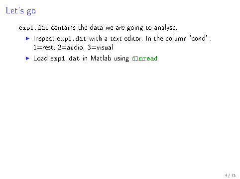
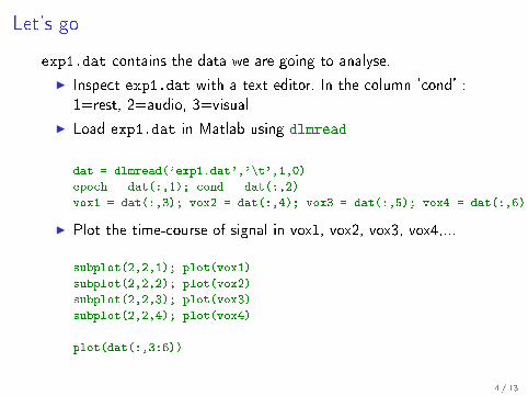
exp1.dat contains the data we are going to analyse.
I Inspect exp1.dat with a text editor. In the column 'cond' :1=rest, 2=audio, 3=visual
I Load exp1.dat in Matlab using dlmread
dat = dlmread('exp1.dat','\t',1,0)
epoch = dat(:,1); cond = dat(:,2)
vox1 = dat(:,3); vox2 = dat(:,4); vox3 = dat(:,5); vox4 = dat(:,6);
I Plot the time-course of signal in vox1, vox2, vox3, vox4,...
subplot(2,2,1); plot(vox1)
subplot(2,2,2); plot(vox2)
subplot(2,2,3); plot(vox3)
subplot(2,2,4); plot(vox4)
plot(dat(:,3:6))
4 / 13

Let's go
exp1.dat contains the data we are going to analyse.
I Inspect exp1.dat with a text editor. In the column 'cond' :1=rest, 2=audio, 3=visual
I Load exp1.dat in Matlab using dlmread
dat = dlmread('exp1.dat','\t',1,0)
epoch = dat(:,1); cond = dat(:,2)
vox1 = dat(:,3); vox2 = dat(:,4); vox3 = dat(:,5); vox4 = dat(:,6);
I Plot the time-course of signal in vox1, vox2, vox3, vox4,...
subplot(2,2,1); plot(vox1)
subplot(2,2,2); plot(vox2)
subplot(2,2,3); plot(vox3)
subplot(2,2,4); plot(vox4)
plot(dat(:,3:6))
4 / 13

I Plot the idealized time-courses of voxels that would respond�perfectly� to audio and to visual stimuli respectively, and to avoxel responding to both.
audio = (cond==2); plot(audio); axis([1 200 -1 2])
visual = (cond==3); plot(visual); axis([1 200 -1 2])
av = (cond==2 | cond==3); plot(av);
I compute the average signal per condition in each voxel
mean(vox1(cond==1)); mean(vox1(cond==2)); mean(vox1(cond==3))
mean(vox2(cond==1)); mean(vox2(cond==2)); mean(vox2(cond==3))
mean(vox3(cond==1)); mean(vox3(cond==2)); mean(vox3(cond==3))
mean(vox4(cond==1)); mean(vox4(cond==2)); mean(vox4(cond==3))
5 / 13

The multiple regression approach (aka �linear model�)
In each voxel, you suppose the response has the form :
voxi = β0 + β1 ∗ audio + β2 ∗ visual + ε
audio = 1 when auditory stim occurs, 0 otherwisevisual = 1 when visual stim occurs, 0 otherwiseε is �noise� with average value of 0.If a voxel does not repond to audio, β1 should be, on average, 0.One can compute a p-value associated to this null hypothesis andreject it if the p-value is small.
6 / 13

Results of multiple regression for each of the four voxels
> display(lm(vox1 ~ cond, data=a))
coef.est coef.se t value Pr(>|t|)
(Intercept) 100.26 0.29 351.32 0.00
cond2 9.77 0.40 24.21 0.00
cond3 -0.11 0.40 -0.28 0.78
> display(lm(vox2 ~ cond, data=a))
coef.est coef.se t value Pr(>|t|)
(Intercept) 99.88 0.29 344.34 0.00
cond2 -0.38 0.41 -0.94 0.35
cond3 15.64 0.41 38.12 0.00
> display(lm(vox3 ~ cond, data=a))
coef.est coef.se t value Pr(>|t|)
(Intercept) 100.09 0.29 350.81 0.00
cond2 4.99 0.40 12.36 0.00
cond3 4.60 0.40 11.40 0.00
> display(lm(vox4 ~ cond, data=a))
lm(formula = vox4 ~ cond, data = a)
coef.est coef.se t value Pr(>|t|)
(Intercept) 99.88 0.26 380.42 0.00
cond2 0.02 0.37 0.06 0.95
cond3 0.09 0.37 0.25 0.80
7 / 13

Design matrix ?I In multiple regression, the �explanatory� variables are the
so-called regressors.I Regrouped into columns, they form the design matrixI In our experiment, the audio and visual conditions are
represented by 0/1 vectors. An intercept is automatically putin the model. It's coe�cient will re�ect the average signal inthe condition which is not modeled (rest).
I Compare the coe�cient estimates with the averages computedearlier.
8 / 13
The (in)famous HRF
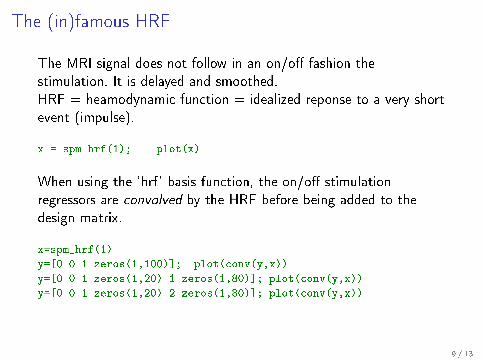
The MRI signal does not follow in an on/o� fashion thestimulation. It is delayed and smoothed.HRF = heamodynamic function = idealized reponse to a very shortevent (impulse).
x = spm_hrf(1); plot(x)
When using the 'hrf' basis function, the on/o� stimulationregressors are convolved by the HRF before being added to thedesign matrix.
x=spm_hrf(1)
y=[0 0 1 zeros(1,100)]; plot(conv(y,x))
y=[0 0 1 zeros(1,20) 1 zeros(1,80)]; plot(conv(y,x))
y=[0 0 1 zeros(1,20) 2 zeros(1,80)]; plot(conv(y,x))
9 / 13

Statistical analysis under SPM
Three steps :
Specify a model Enter the information describing the design of theexperiment : how many sessions, how manyexperimental conditions, the onsets and durations ofevents for each condition,...This creates the design matrix.
Estimate a model Given the design matrix and the functional scans,this step computes, for each voxel, the coe�cients
associated to each regressor in the design matrix.
Results Create and inspect contrasts to compare thecoe�cients associated to di�erent conditions.
10 / 13

Exercice : Specifying a model for a bloc design
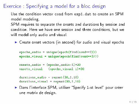
Use the condition vector cond from exp1.dat to create an SPMmodel modeling.SPM requires to separate the onsets and durations by session andcondition. Here we have one session and three conditions, but wewill model only audio and visual.
I Create onset vectors (in second) for audio and visual epochs
epochs_audio = unique(epoch(find(cond==2)))
epochs_visual = unique(epoch(find(cond==3)))
onsets_audio = (epochs_audio-1)*30
onsets_visual = (epochs_visual-1)*30
durations_audio = repmat(30,1,10)
durations_visual = repmat(30,1,10)
I Dans l'interface SPM, utiliser �Specify 1-st level� pour créerune matrix de design.
11 / 13
Exercice : Specifying a model for a bloc design
Use the condition vector cond from exp1.dat to create an SPMmodel modeling.SPM requires to separate the onsets and durations by session andcondition. Here we have one session and three conditions, but wewill model only audio and visual.
I Create onset vectors (in second) for audio and visual epochs
epochs_audio = unique(epoch(find(cond==2)))
epochs_visual = unique(epoch(find(cond==3)))
onsets_audio = (epochs_audio-1)*30
onsets_visual = (epochs_visual-1)*30
durations_audio = repmat(30,1,10)
durations_visual = repmat(30,1,10)
I Dans l'interface SPM, utiliser �Specify 1-st level� pour créerune matrix de design.
11 / 13

Results
A (T) contrast is a set of weights ωi associated to the coe�cientsβi .The value of a contrast is the scalar product :
∑iωi ∗ βi .
From the data, one can compute a standard error, and therefore aT and p-value associated to a contrast.Consider a design matrix with two regressors, audio and visual,followed by the intercept.
I Voxels responding to audio (more than rest) : [1 0 0]
I Voxels responding to visual (more than rest) : [0 1 0]
I Voxels responding more to audio than visual : [1 -1 0]
I Voxels responding more to rest than to audio : ?
12 / 13
13 / 13