introduction to matlab - serveur pédagogique ufr...
TRANSCRIPT


Sources
Based on courses from:
Faouzi Alaya Cheikh, høgskolen i Gjøvik
Emmanuel Marin, University of Saint-Etienne
Yacine Bouroubi, University of Montreal
Alastair McAndrew, Victoria University of technology
3
Outline
Introduction Run and quit MATLAB
environment
Help
Variables Matrices/vectors
Built-in Variables
Operations and Functions Operations
Linear Algebra
Functions
String of characters
Graphics
Programming Scripts and Data Management
Functions
Matlab & Image Processing
Introduction
Image Types
Converting Between Image Types
Converting Between Image Classes
histograms
Color space conversion
Image Arithmetic
Working with Image Sequences

4
Introduction
MATLAB (stands for “Matrix laboratory”) is an environment suited for working with arrays and matrices.
Main advantages: Simple of use because of the vectorization.
Computational power.
Results accuracy.
It integrates: computing, programming and visualization.
It can be run on any type of computer or environment (PC, windows/UNIX, Macintosh, working station…)
A basic tool, but Several toolboxes (i.e. sets of predefined functions) are available, focusing on different engineering fields: statistics, signal processing, image processing, wavelets, control, data acquisition ...

Introduction
For specific applications it offers the same possibilites of structured programmation as other languages (C, C++, FORTRAN…).
It is written in optimized C language and contains part in assambling language for better performances.
MATLAB can be used both from the command line window and by running scripts stored in “.m” files.
Data can be saved in files that end in “.mat”.
GUI‟s are available for specific tasks.
Limits of this course: Introduce the basics
Show some practical examples in image processing
Practice, practice, practice
Visit http://www.mathworks.com for more on MATLAB.
5

Introduction: Run and quit
Windows Double click the .exe in the MATLAB directory
Start/Programs/MATLAB/…/MATLAB
Quit with scroll menu File/Quit or with shortcuts Alt+F4…
Quit typing exit
UNIX Type matlab to run
The command window is open and permits to write commands, execute calculus or run programs
6
7
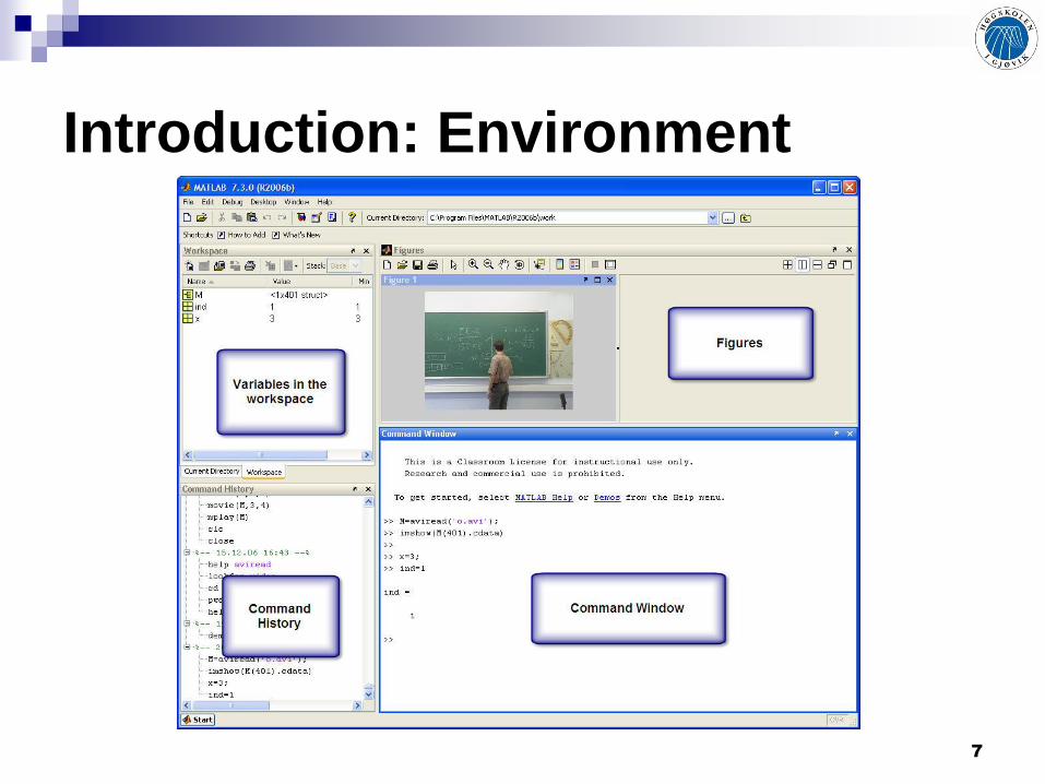
Introduction: Environment

Introduction: First step
Type: >> A=5
>> B=[1 2 3 ; 4 5 6];
>> C=[7 , 8 ; 9 , 10 ; 11 , 12]
>> B*C
>> B.*C
>> B.*C‟
>> B^2
>> B.^2
>> A*B
>> A.*B
>> mean(B)
>>mean(mean(B))
MATLAB deals with different types of data often with the same operators or functions (polymorphism). Then the result of an operation depends on the type of data.
8

9
Help
In-line help is really clear and complete
Quick help can be obtained in MATLAB:
help, help command, help dir, lookfor command, helpwin, helpdesk, lookfor keyword, whatsnew.
Try type command.
To get an overview of what you can do using MATLAB type: demo(s)
Try with the commands plot and/or mean
10
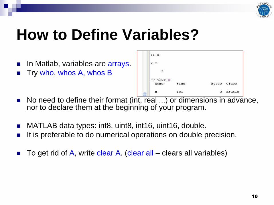
How to Define Variables?
In Matlab, variables are arrays.
Try who, whos A, whos B
No need to define their format (int, real ...) or dimensions in advance, nor to declare them at the beginning of your program.
MATLAB data types: int8, uint8, int16, uint16, double.
It is preferable to do numerical operations on double precision.
To get rid of A, write clear A. (clear all – clears all variables)
11
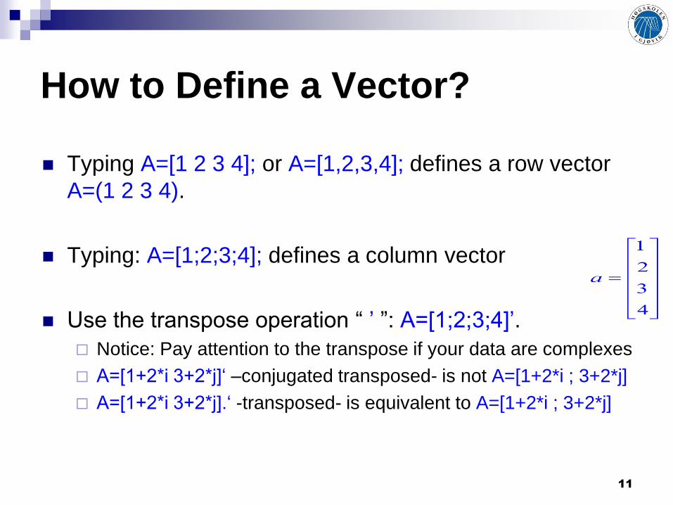
How to Define a Vector?
Typing A=[1 2 3 4]; or A=[1,2,3,4]; defines a row vector
A=(1 2 3 4).
Typing: A=[1;2;3;4]; defines a column vector
Use the transpose operation “ ‟ ”: A=[1;2;3;4]‟.
Notice: Pay attention to the transpose if your data are complexes
A=[1+2*i 3+2*j]„ –conjugated transposed- is not A=[1+2*i ; 3+2*j]
A=[1+2*i 3+2*j].„ -transposed- is equivalent to A=[1+2*i ; 3+2*j]

12
How to Define a Matrix?
A matrix is a stack of row vectors. Type A=[1 2 3; 1 2 3] to create a 2×3 matrix:
To access the (i,j) element of a, just type A(i,j).
For instance A(2, 3) will return ans = 3.
Elements of a matrix can also be reassigned, e.g. A(2, 3)=50; transforms A in to:
What is A(:,:), A(1:2,2:3), A(6), A(2,:), A(:,2), A(:)?
3
3
2
2
1
1A
50
3
2
2
1
1A

Defining Vectors
“:” is used to represent a serie of values. t=i:j:k. A set of numbers from I to k by step of j.
Type t=[0:.1:1] or t=0:.1:1. Defines a row vector t whose elements range from 0 to 1 and are spaced by 0.1.
Type t=[0:.12:1]. The last value is <=k
Linear or logarithmic distribution can be created using linspace(a,b), linspace(a,b,n) 100 or n values in [a,b]
logspace(a,b), logspace(a,b,n) 50 or n values in [10a,10b]
13
14
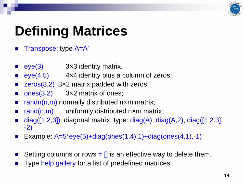
Defining Matrices Transpose: type A=A‟
eye(3) 3×3 identity matrix.
eye(4,5) 4×4 identity plus a column of zeros;
zeros(3,2) 3×2 matrix padded with zeros;
ones(3,2) 3×2 matrix of ones;
randn(n,m) normally distributed n×m matrix;
rand(n,m) uniformly distributed n×m matrix;
diag([1,2,3]) diagonal matrix, type: diag(A), diag(A,2), diag([1 2 3], -2)
Example: A=5*eye(5)+diag(ones(1,4),1)+diag(ones(4,1),-1)
Setting columns or rows = [] is an effective way to delete them.
Type help gallery for a list of predefined matrices.

15
Managing Matrices [N,M]=size(A) returns the row and cols number of A. size(A,2) for the cols
number.
length(A), returns the bigger number between the number of rows and the number of columns.
[Y,I]=max(A) returns: Y maximum elt. In each cols of A; I, indices of the corresponding elt.. max(max(A)) returns the maximum element of A.
[Y,I]=min(A), same principle.
Y=sort(A), sorts the cols of A in ascending or descending order. Type help sort
find(M==1) returns the linear indices of the elt == 1.
Try help elmat to see the full list of Elementary matrices and matrix manipulations.
16
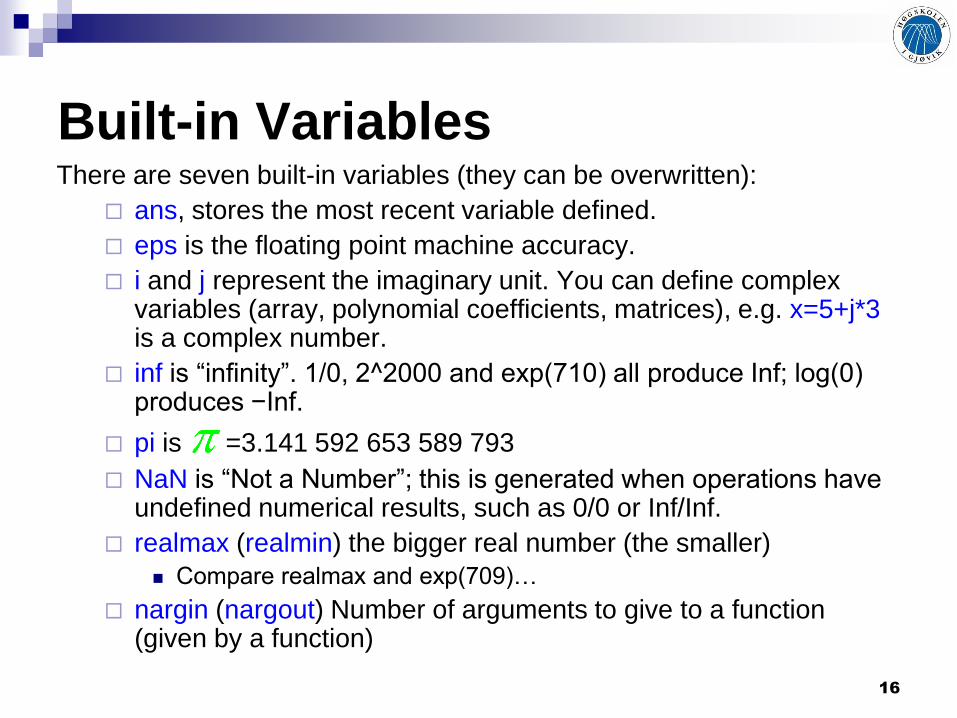
Built-in Variables There are seven built-in variables (they can be overwritten):
ans, stores the most recent variable defined.
eps is the floating point machine accuracy.
i and j represent the imaginary unit. You can define complex variables (array, polynomial coefficients, matrices), e.g. x=5+j*3 is a complex number.
inf is “infinity”. 1/0, 2^2000 and exp(710) all produce Inf; log(0) produces −Inf.
pi is =3.141 592 653 589 793 NaN is “Not a Number”; this is generated when operations have
undefined numerical results, such as 0/0 or Inf/Inf.
realmax (realmin) the bigger real number (the smaller)
Compare realmax and exp(709)…
nargin (nargout) Number of arguments to give to a function (given by a function)

17
Operations & Functions
can
18
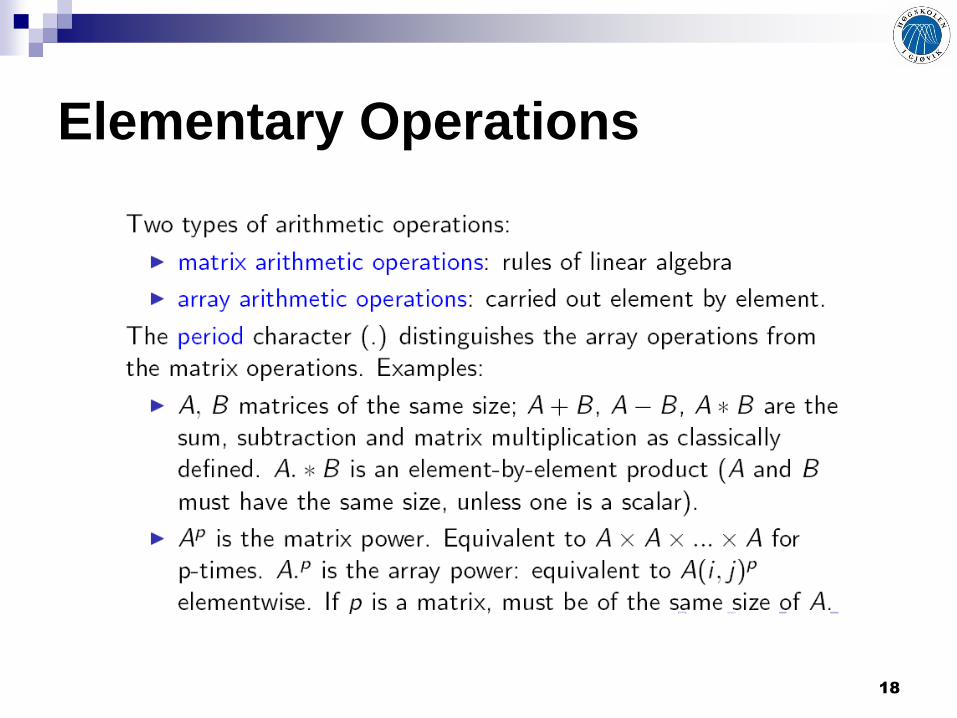
Elementary Operations

19
Elementary Vector Operations
20
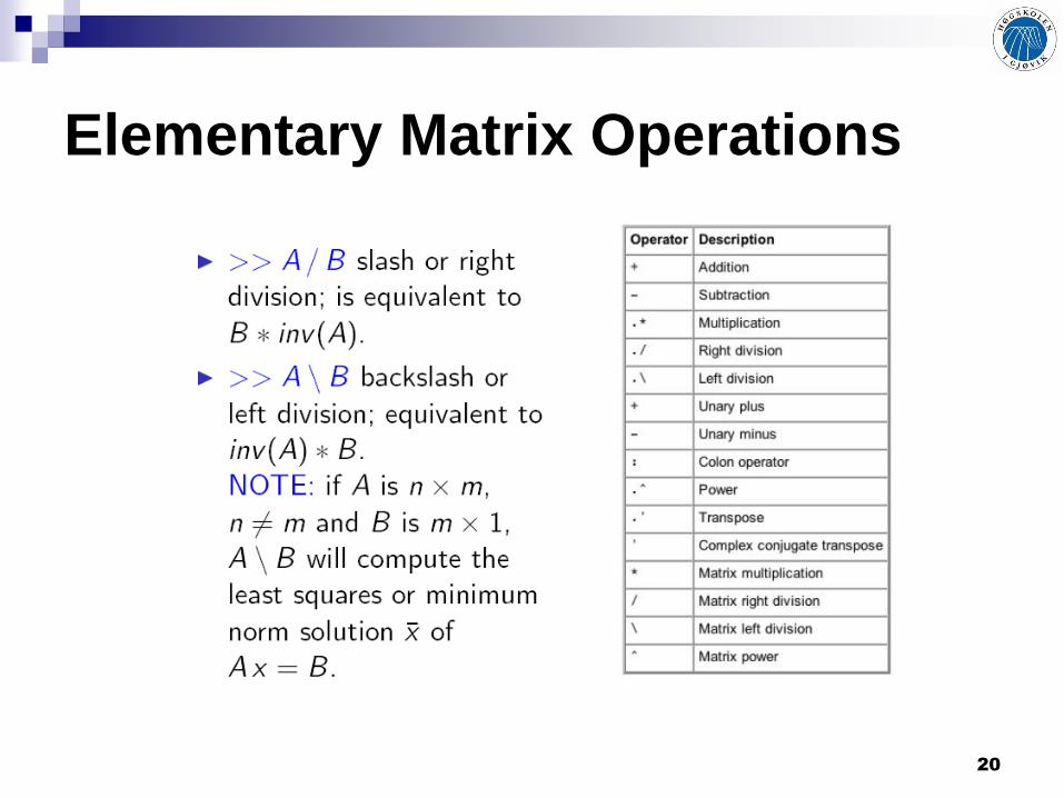
Elementary Matrix Operations

Elementary Matrix Operations
dot(A, B) scalar product
cross(A, B) vectorial product
kron(A, B) tensorial product
Check the help
21

22
Relational Operations

23
Logic Operations

24
Linear Algebra
25
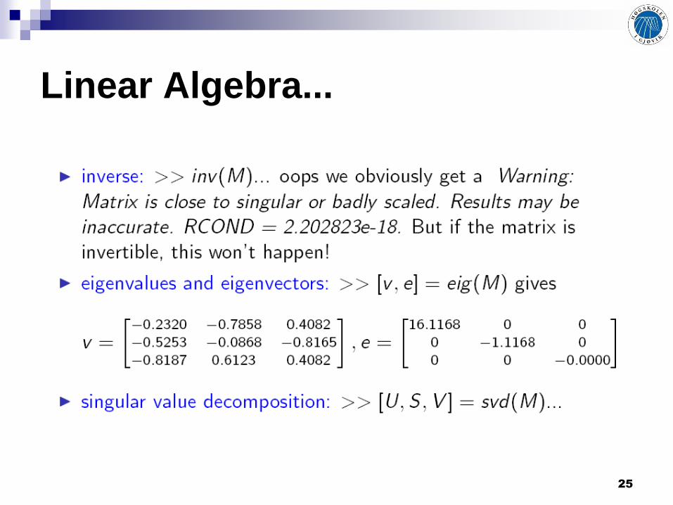
Linear Algebra...

26
Other Math Functions
|x|
1, -1 ou 0
x
abs(x) sign(x) sqrt(x) pow2(x, f)
x*2f exp(x) log(x) log10(x) log2(x)
e x
base e
base 10
base 2
sin(x) cos(x) tan(x) cot(x) sec(x)
x in rad
1/cos(x)
asin(x) acos(x) atan(x) atan2(x,y) acot(x)
arc in rad
atan(x/y), [- , + ]
Check with help
Hyperbolic functions
sinh(x) ...
Inverted hyperbolic functions
asinh(x) ...
Rounded values ... round(x) fix(x) floor(x)
ceil(x) gcd(x, y) lcm(x, y) rat(x)

Other Math Functions
Functions for complexes
Given z=x+yi=r*eth*i
Example:
z=1+2i ;
x=real(z), y=imag(z), r=abs(z), zc=conj(z), th=angle(z) ;
m=[x y r zc th] '
Coordinates shift
[th,r]=cart2pol(x,y), [x,y]=pol2cart(th,r),
[al,th,r]=cart2sph(x,y,z), [x,y,z]=sph2cart(al,th,r)
27

28
Example: Rounding Functions
fix(X) rounds the elements of X to the nearest integers towards zero.
round(X) rounds the elements of X to the nearest integers.
ceil(X) rounds the elements of X to the nearest integers towards infinity.
floor(X) rounds the elements of X to the nearest integers towards minus infinity.
Example: Applying the previous functions to X = [-1.5 -1.49 1.49 1.5]
results in:
fix(X) = [ -1 -1 1 1 ] round(X) = [ -2 -1 1 2 ]
ceil(X) = [ -1 -1 2 2 ] floor(X) = [ -2 -2 1 1 ]
Note that fix behaves as ceil when X < 0 and as floor when X > 0.

Data and function analysis
Given k a scalar, x a vector and A a matrix sum(x), sum(A)
cumsum(x), cumsum(A)
prod(x)
diff(x), diff(A), diff(x,k)
mean(x), mean(A)
median(x), median(A)
std(x), std(A)
var(x), var(A)
…
polyval, poly, roots, fzero, fmin, polfit…
interp1, interp2, interp3…
fft, fft2…
29

Character’s string
A character string is defined by ‟…‟
my_text=‟**This is a string of 35 elements**‟
check=length(my_text)
check=
35 Or I made a mistake ;)
The text is memorized as a row vector which each elt contains the ANSCII code for the symbol. my_text(3)=‟t‟
disp(my_text); Input(my_text) input(my_text, ‟s‟)
n=input(‟Give a number : ‟)
give a number : 5.123
A=input(‟Enter a matrix row by row : ‟) ;
Enter a matrix row by row : [1 :3 ; 4 7 8]
n=
5.1230
A=input(‟Enter a matrix : ‟) ;
Enter a matrix : rand(4)*hilb(4)
[m n]=input(‟Give the size of A : ‟) ;
Give the size of A : size(A)
login=input(‟what is your login name ? ‟, ‟s‟) ;
What is your login name ? RabbitRoger
30
31
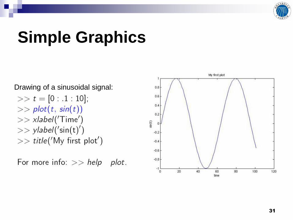
Simple Graphics
Drawing of a sinusoidal signal:

32
Simple Graphics
To draw one circle of radius 1, use the following code:
t = 0:pi/100:2*pi;
plot(sin(t), cos(t));
t = linspace(0,2*pi,200); is another way of getting 200 points between 0 and 2*pi
If you want to add another circle of radius 0.5, how would you do it?

33
Surfaces
34
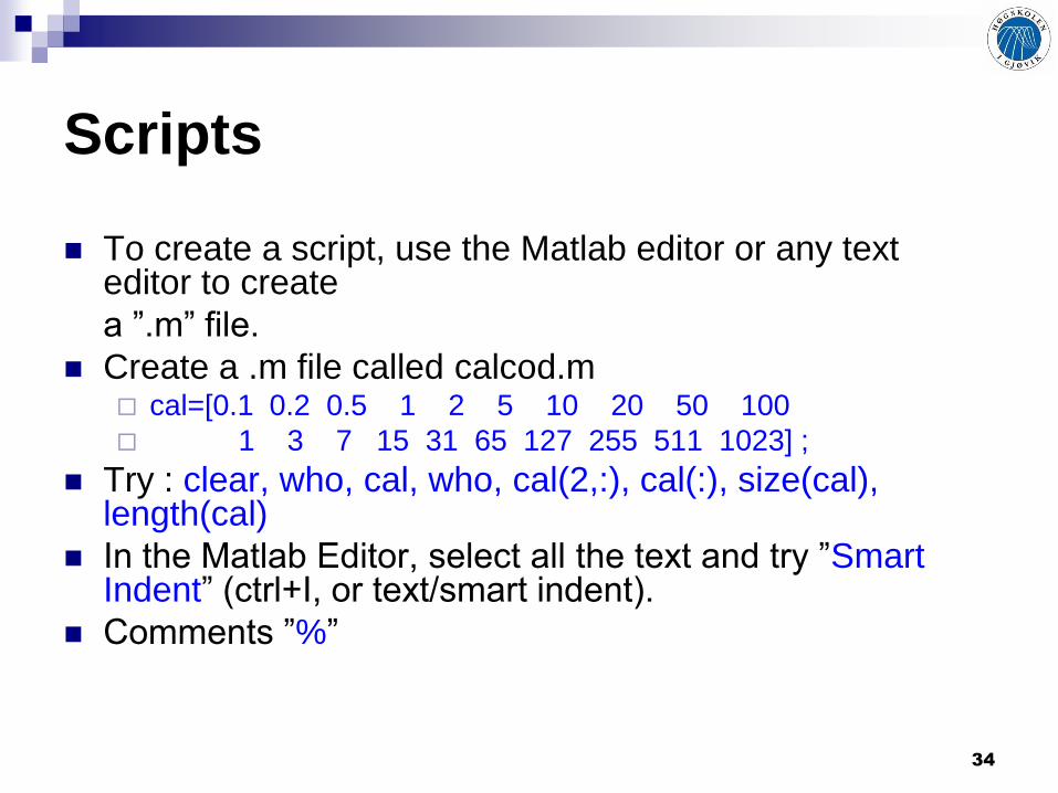
Scripts
To create a script, use the Matlab editor or any text editor to create
a ”.m” file.
Create a .m file called calcod.m cal=[0.1 0.2 0.5 1 2 5 10 20 50 100
1 3 7 15 31 65 127 255 511 1023] ;
Try : clear, who, cal, who, cal(2,:), cal(:), size(cal), length(cal)
In the Matlab Editor, select all the text and try ”Smart Indent” (ctrl+I, or text/smart indent).
Comments ”%”

35
Save and load data
save % save variables in a binary file save filename % in filename.mat
save filename a b % only the variables a and b
save filename.dat v1 v2 –ascii % in ascii format
load % read a binary file load filename
load filename.dat v1 v2
Example: a data file:A.dat, containing the matrix
1 4 5
4 2 9 load A.dat; A
The variable take the name of the file.
See also: fread, fwrite
wk1read, wk1write
dlmread, dlmwrite

36
Functions To create a function:
The first line begin by function, following by the output arguments, the name of the function, and formal parameters within parenthesis.
The name of the file and the name of the function HAVE to be the same
Calling the function is done with real arguments designed by independent names
Comments with %, put just after the first line they will be displayed with help
Example: function y=lnesin(x)
% lnesin : compute the expression exp(-x^2)+sin((x^2)/5)
% parameter x : scalar or vector
% y, the out argument is of the same type
y= exp(-x.^2)+sin(0.2*x.^2) ;
end ;
In command line (file/set path), type: >> x1=[-10 :0.1 :10] ;
>> f1=lnesin(x1) ;
>> plot(x1, f1) ;
>> help lnesin

Flow Control
switch exists also…
37

Flow control, example
given a vector v, create a new vector with values equal to v if they are greater than 0, and equal to 0 if they less than or equal to 0.
using a FOR loop v = [3 5 -2 5 -1 0]
u = zeros( size(v) ); % initialize
for i = 1:size(v,2)
if( v(i) > 0 )
u(i) = v(i);
end
end
u
without FOR loop v = [3 5 -2 5 -1 0]
u2 = zeros( size(v) ); % initialize
ind = find( v>0 ) % index into >0 elements
u2(ind) = v( ind )
With MATLAB, it is always better to limit the use of for loops (slow and not nice). You would rather find the formulation of the problem which permits to use built in functions.
38

39
Image Processing in Matlab IPTB
Images in MATLAB and the Image Processing Toolbox How images are represented in MATLAB and the Image Processing
Toolbox
Image Types in the Toolbox Fundamental image types supported by the Image Processing Toolbox
Converting Between Images Converting between the image types
Converting Between Image Classes
Converting image data from one class to another
Image Arithmetic Adding, subtracting, multiplying, and dividing images
Working with Image Sequences

40
Image Processing in Matlab IPTB...
The basic data structure in MATLAB is the array, an ordered set of real or
complex elements. This object is naturally suited to the representation of images, real-valued ordered sets of color or intensity data.
MATLAB stores most images as two-dimensional arrays (i.e., matrices), in
which each element of the matrix corresponds to a single pixel in the displayed
image. (Pixel is derived from picture element and usually denotes a single dot on a computer display.)
Try: help images, imdemos, imuitools, iptutils, medformats.
http://www.mathworks.com/access/helpdesk/help/toolbox/images/

41
First step
Read an image: I = imread('pout.tif');
Display an image: imshow(I), imtool(I)
Try: whos I, imfinfo('pout.tif'), impixelinfo
Try these commands: figure, imhist(I)
I2=histeq(I);
figure, imshow(I2)
figure, imhist(I2)
imwrite (I2, 'pout2.png');

42
Pixel Coordinate System
I(r, c)
For example, the I(2,15) returns the value of the
pixel at row 2, column 15 of the image I.

43
Image Types
MATLAB IPTB defines 4 image types
Binary
(bi-level image)
Logical array containing only 0s and 1s, interpreted as black and white, respectively.
Indexed
(pseudo-color image)
Array of class logical, uint8, uint16, single, or double whose pixel values are
Direct indices into a colormap. The colormap is an m-by-3 array of class double.
For single or double arrays, integer values range from [1, p]. For logical, uint8, or
uint16 arrays, values range from [0, p-1].
Gray-scale
(intensity image)
Array of class uint8, uint16, int16, single, or double whose pixel values specify
intensity values. For single or double arrays, values range from [0, 1].
For uint8, values range from [0,255]. For uint16, values range from [0, 65535].
For int16, values range from [-32768, 32767].
True-color
(RGB image )
m-by-n-by-3 array of class uint8, uint16, single, or double whose pixel values
specify intensity values. For single or double arrays, values range from [0,1].
For uint8, values range from [0, 255]. For uint16, values range from [0, 65535].

44
Binary Images
Binary image ~ Logical Array of 0 & 1.

45
Indexed Images
Consists of an array “X” and a colormap “map” matrix.
The pixel values in “X” are direct indices into the colormap.
Each colormap matrix row (values in [0,1])
specifies the RGB components of a single color
in the image.
Red Green Blue

www.hig.no/~faouzi 46
Gray-Scale Images
A gray-scale image is a data matrix whose values represent intensities within some range.
The matrix can be of class uint8, uint16, int16, single, or double.
While grayscale images are rarely saved with a colormap, MATLAB uses a colormap to display them.

47
True-color Images
A true-color image is an image in which each pixel is specified by
three values: the red, green and blue components of the pixel‟s
color.
MATLAB stores true-color images as an m-by-n-by-3 data array,
with no color map.
For example, the red, green, and blue color components of the pixel
(10,5) are stored in I(10,5,1), I(10,5,2), and I(10,5,3), respectively.
A true-color array can be of class uint8, uint16, single, or double.

48
True-color Images

49
Basic Functions...
Resizing
imresize changes the size of the image
A=imresize(I,.5);
Rotation
imrotate rotates the image by given angle
Cropping
imcrop Extract a rectangular part of the image

50
True-Color Images
Try this: RGB=reshape(ones(64,1)*reshape(jet(64),1,192),[64,64,3]);
R=RGB(:,:,1);
G=RGB(:,:,2);
B=RGB(:,:,3);
figure, imshow(RGB), title('True Color')
figure, imshow(B), title('Blue')
figure, imshow(G), title('Green')
figure, imshow(R), title('Red')

Exercise: Histogram Example: histogram
1D / represent the frequence of occurence of a greylevel I=Imread(‟cameraman.tif‟);
figure, imhist(I);
I2=histeq(I);
figure, imshow(I2)
figure, imhist(I2)
2D / represent the coocurrence of the combination of two pixels of the same intensities, given a distance and a direction glcm = graycomatrix(I,'Offset',[0 0], 'NumLevels',256);
imtool(glcm./ max(max(glcm)))
glcm = graycomatrix(I,'Offset',[-1 1], 'NumLevels',256);
Imtool(glcm./max(max(glcm)))
Imtool(log(glcm)./log(max(max(glcm))))
2D histograms can be computed for 2 images of the same size, or between 2 layers of a same color image.
Cf. K. Frank lecture
51

52
Convert Between Image Types
Also try: RGB = cat(3,I,I,I); with I being a gray-scale image.

53
Indexed Images [x,map] = imread('trees.tif');
Imshow(x)
imshow(x,map)
imtool(x, map)
Imtool(x,jet)

54
Convert Indexed to Intensity Images
image = ind2gray(x,map);
imtool(image)
imtool(x)
55
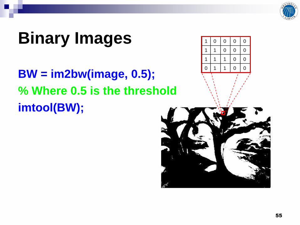
Binary Images
BW = im2bw(image, 0.5);
% Where 0.5 is the threshold
imtool(BW);
1 0 0 0 0
1 1 0 0 0
1 1 1 0 0
0 1 1 0 0

56
Convert Between Image Classes
Converting between classes changes the way MATLAB and the toolbox interpret the image data.
To be interpreted properly as image data, you need to rescale or offset the data when you convert it.
To avoid problems of type, use one of these toolbox functions: im2uint8, im2uint16, im2int16, im2single, or im2double.
Class converting problems: Converting to a class that uses fewer bits to represent numbers,
generally implies some loss of the image information.
Not always possible to convert an indexed image from one storage class to another.
57
Color Space Conversions
The Image Processing Toolbox represents colors as RGB values in both True-color and indexed images.
The toolbox provides functions to convert between color spaces.
The image processing functions themselves assume all color data is RGB.

58
Color Space Conversions

59
Color Space Conversions

60
Color Space Conversions
Conversion Example:
Read image:
rgb = imread('peppers.png');
Create a color transformation structure that defines a
conversion from RGB color data to XYZ color data:
C = makecform('srgb2xyz');
Use the applycform function to perform the conversion:
xyz = applycform(rgb,C);

61
The toolbox includes functions that you can use to convert RGB data to several common device-dependent color spaces, and vice versa: YIQ
YCbCr
Hue, saturation, value (HSV)
RGB = imread('peppers.png');
%process only along the intensity
>>cn=rgb2ntsc(RGB); %convert to YIQ color space where Y (intensity) can be isolated
>>cn(:,:,1)=histeq(cn(:,:,1)); %perform histogram equalization on the intensity.
>>imtool(cn)
>>c2=ntsc2rgb(cn);
>> imshow(c2);
%process along each channel independently
>> cr= histeq(RGB(:,:,1));
>> cg= histeq(RGB(:,:,2));
>> cb= histeq(RGB(:,:,3));
>> c3=cat(3,cr,cg,cb);
>> Imtool(c3)
Converting Between Device-Dependent
Color Spaces

62
Image Arithmetic
MATLAB arithmetic operators and the IPTB arithmetic functions use these rules for integer arithmetic: Values that exceed the range of the integer type are saturated to that
range.
Fractional values are rounded.
Therefore, avoid nesting calls to image arithmetic functions!
Example: calculate the average of two images, I = imread('rice.png');
I2 = imread('cameraman.tif');
K = imdivide(imadd(I,I2), 2); % not recommended
When used with uint8 or uint16 data, each arithmetic function rounds and saturates its result before passing it on to the next operation. This can significantly reduce the precision of the calculation. K = imlincomb(.5,I,.5,I2); % recommended

63
Image Arithmetic…
Applying an image arithmetic operation on two images A and B or on a constant c and an image A: Adding:
Imadd(A, B), imadd(A, c)
Subtracting
imsubtract(A, B), imsubtract(A, c)
Multiplying
Immultiply(A, B), immultiply(A, c)
Dividing
Imdivide(A, B), imdivide(A, c)

64
Working with Image Sequences
Image sequences are collections of images related: by time: frames in a movie,
or by view (spatial location): such as MRI slices.
An m-by-n-by-p array can store p, 2-D grayscale or binary images.
An m-by-n-by-3-by-p array can store p, true-color images.

65
Example:
load mri
whos
mov = immovie(D,map);
movie(mov,3)
Working with Image Sequences

66
Multidimensional Arrays as
Image Sequences
Many toolbox functions can operate on multi-dimensional arrays and, consequently, can operate on image sequences.
For example, if you pass a multi-dimensional array to the imtransform function, it applies the same 2-D transformation to all
2-D planes along the higher dimension.
Some functions, however, do not by default interpret an m-by-n-by-p or an m-by-n-by-3-by-p array as an image sequence.

67
IPTB Functions for 4-D Arrays

68
IPTB Functions for 4-D Arrays

69
Multi-Frame Image Arrays
The IPTB includes two functions, immovie and montage, that work with a specific type of multi-dimensional array called a multi-frame array. In this array, images, called frames in this context, are concatenated along the fourth dimension.
Multi-frame arrays are either: m-by-n-by-1-by-p, for grayscale, binary, or indexed images,
m-by-n-by-3-by-p, for true-color images, where p is the number of frames.
For example, a multi-frame array containing 5, 480-by-640 grayscale or
indexed images would be 480-by-640-by-1-by-5. An array with 5, 480-by-640 truecolor images would be 480-by-640-by-3-by-5.

70
Multi-Frame Image Arrays
Use the cat command to create a multi-frame array. For example, to store a group of images (A1, A2, A3, A4, and A5) in a single array. A = cat(4, A1, A2, A3, A4, A5)
To extract frames from a multi-frame image MULTI: FRM3 = MULTI(:,:,:,3)
Note: In a multi-frame image array, each image must be the same size
and have the same number of planes. In a multi-frame indexed image, each image must also use the same
color-map.

71
Conclusions
This was a short introduction to the main
features of MATLAB and the IPTB.
More can be found in:
The embedded help, help
http://www.mathworks.com
http://www.mathworks.com/matlabcentral
Google ...