introduction to matrix algebra -...
TRANSCRIPT

Introduction to
MATRIX ALGEBRA©
KAW © Copyrighted to Autar K. Kaw – 2002
1
Introduction to
MATRIX ALGEBRA
Autar K. Kaw University of South Florida
Autar K. Kaw
Professor & Jerome Krivanek Distinguished Teacher
Mechanical Engineering Department
University of South Florida, ENB 118
4202 E. Fowler Avenue
Tampa, FL 33620-5350.
Office: (813) 974-5626
Fax: (813) 974-3539
E-mail: [email protected]: http://www.eng.usf.edu/~kaw
2
Table of Contents Chapter 1: Introduction …………………………………………..… 6 What is a matrix?So what is a matrix?What are the special types of matrices?Do non-square matrices have diagonal entries?When are two matrices considered to be equal?KEYTERMS CH1 Chapter 2: Vectors ………………………………………………… 20 What is a vector?When are two vectors equal?How do you add two vectors?What is a null vector?What is a unit vector?How do you multiply a vector by a scalar?What do you mean by a linear combination of vectors?What do you mean by vectors being linearly independent?What do you mean by the rank of a set of vectors?How can vectors be used to write simultaneous linear equations?What is the definition of the dot product of two vectors?KEYTERMS CH2 Chapter 3: Binary Matrix Operations …………………………… 41 How do you add two matrices?How do you subtract two matrices?How do I multiply two matrices?What is a scalar product of a constant and a matrix?What is a linear combination of matrices?What are some of the rules of binary matrix operations?KEYTERMS CH3 Chapter 4: Unary Matrix Operations …………………………… 55 What is a skew-symmetric matrix?How does one calculate the determinant of any square matrix?Is there a relationship between det (AB), and det (A) and det (B)?Are there some other theorems that are important in finding the determinant?KEYTERMS CH4 Chapter 5: System of Equations …………………………………. 72 Matrix algebra is used for solving system of equations. Can you illustrate this concept?A system of equations can be consistent or inconsistent. What does that mean?
3
How can one distinguish between a consistent and inconsistent system of equations?But, what do you mean by rank of a matrix?If a solution exists, how do we know whether it is unique?If we have more equations than unknowns in [A] [X] = [C], does it mean the system is inconsistent?Consistent system of equations can only have a unique solution or infinite solutions. Can a system of equations have a finite (more than one but not infinite) number of solutions?Can you divide two matrices?How do I find the inverse of a matrix?Is there another way to find the inverse of a matrix?If the inverse of a square matrix [A] exists, is it unique? KEYTERMS CH5 Chapter 6: Gaussian Elimination ………………………………… 107 How are a set of equations solved numerically?Are there any pitfalls of Naïve Gauss Elimination Method?What are the techniques for improving Naïve Gauss Elimination Method? How does Gaussian elimination with partial pivoting differ from Naïve Gauss elimination?Can we use Naïve Gauss Elimination methods to find the determinant of a square matrix?KEYTERMS CH6 Chapter 7: LU Decomposition ………………………………….… 129 I hear about LU Decomposition used as a method to solve a set of simultaneous linear equations? What is it and why do we need to learn different methods of solving a set of simultaneous linear equations?
How do I decompose a non-singular matrix [A], that is, how do I find [ ] ?[ ][ ]U LA =
How do I find the inverse of a square matrix using LU Decomposition?KEYTERMS CH7 Chapter 8: Gauss- Seidal Method………………………………… 144 Why do we need another method to solve a set of simultaneous linear equations? Chapter 9: Adequacy of Solutions………………………………… 158 What does it mean by ill conditioned and well-conditioned system of equations?So what if the system of equations is ill conditioning or well conditioning?To calculate condition number of an invertible square matrix, I need to know what norm of a matrix means. How is the norm of a matrix defined?How is norm related to the conditioning of the matrix?What are some of the properties of norms?
Is there a general relationship that exists between C/CandX/X ΔΔ or between X/XΔ and A/AΔ ? If so, it could help us identify well-conditioned and ill
conditioned system of equations.
4

If there is such a relationship, will it help us quantify the conditioning of the matrix, that is, tell us how many significant digits we could trust in the solution of a system of simultaneous linear equations?How do I use the above theorems to find how many significant digits are correct in my solution vector?KEYTERMS CH9 Chapter 10: Eigenvalues and Eigenvectors …………………….. 173 What does eigenvalue mean?Can you give me a physical example application of eigenvalues and eigenvectors?What is the general definition of eigenvalues and eigenvectors of a square matrix?How do I find eigenvalues of a square matrix?What are some of the theorems of eigenvalues and eigenvectors?How does one find eigenvalues and eigenvectors numerically?KEYTERMS CH10
5

6

Chapter 1 Introduction _________________________________ After reading this chapter, you should be able to
Know what a matrix is
Identify special types of matrices
When two matrices are equal
_________________________________ What is a matrix?
Matrices are everywhere. If you have used a spreadsheet such as Excel or Lotus or written a table, you have used a matrix. Matrices make presentation of numbers clearer and make calculations easier to program. Look at the matrix below about the sale of tires in a Blowoutr’us store – given by quarter and make of tires.
Quarter 1 Quarter 2 Quarter 3 Quarter 4
CopperMichiganTirestone
⎢⎢⎢
⎣
⎡
6525
161020
7
153
⎥⎥⎥
⎦
⎤
27252
If one wants to know how many Copper tires were sold in Quarter 4, we go along the row ‘Copper’ and column ‘Quarter 4’ and find that it is 27.
So what is a matrix?
A matrix is a rectangular array of elements. The elements can be symbolic expressions or numbers. Matrix [A] is denoted by
[ ]⎥⎥⎥⎥
⎦
⎤
⎢⎢⎢⎢
⎣
⎡
=
mnmm
n
n
aaa
aaaaaa
A
.......
.......
.......
21
22221
11211
MM
Row i of [A] has n elements and is [ ]inii aaa ....2 1 and
7
Column j of [A] has m elements and is
⎥⎥⎥⎥⎥
⎦
⎤
⎢⎢⎢⎢⎢
⎣
⎡
mj
j
j
a
aa
M2
1
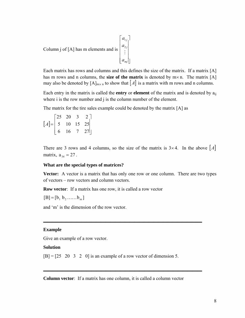
Each matrix has rows and columns and this defines the size of the matrix. If a matrix [A] has m rows and n columns, the size of the matrix is denoted by m×n. The matrix [A] may also be denoted by [A]m× n to show that [ ]A is a matrix with m rows and n columns.
Each entry in the matrix is called the entry or element of the matrix and is denoted by aij where i is the row number and j is the column number of the element.
The matrix for the tire sales example could be denoted by the matrix [A] as
[ ]⎥⎥⎥
⎦
⎤
⎢⎢⎢
⎣
⎡=
2771662515105232025
A
There are 3 rows and 4 columns, so the size of the matrix is 3×4. In the above [ ]A matrix, . 27a 34 =
What are the special types of matrices?
Vector: A vector is a matrix that has only one row or one column. There are two types of vectors – row vectors and column vectors.
Row vector: If a matrix has one row, it is called a row vector
]bbb[]B[ m21 KK=
and ‘m’ is the dimension of the row vector.
_________________________________ Example
Give an example of a row vector.
Solution
[B] = [25 20 3 2 0] is an example of a row vector of dimension 5.
_________________________________ Column vector: If a matrix has one column, it is called a column vector
8

[ ]⎥⎥⎥⎥
⎦
⎤
⎢⎢⎢⎢
⎣
⎡
=
n
1
c
c
CM
M
and n is the dimension of the vector.
_________________________________ Example
Give an example of a column vector.
Solution
[ ] is an example of a column vector ⎥⎥⎥
⎦
⎤
⎢⎢⎢
⎣
⎡=
6525
C
of dimension 3.
_________________________________ Submatrix: If some row(s) or/and column(s) of a matrix [A] are deleted (no rows or columns may be deleted), the remaining matrix is called a submatrix of [A].
Example
Find some of the submatrices of the matrix
[ ] ⎥⎦
⎤⎢⎣
⎡−
=213264
A
Solution
[ ] [ ] ⎥⎦
⎤⎢⎣
⎡⎥⎦
⎤⎢⎣
⎡−⎥
⎦
⎤⎢⎣
⎡− 2
2,4,264,
1364
,213264
are some of the submatrices of [A]. Can you find
other submatrices of [A]?
_________________________________ Square matrix: If the number of rows (m) of a matrix is equal to the number of columns (n) of the matrix, (m = n), it is called a square matrix. The entries a11, a22, . . . ann are
9

called the diagonal elements of a square matrix. Sometimes the diagonal of the matrix is also called the principal or main of the matrix.
_________________________________ Example
Give an example of a square matrix.
Solution
[ ]⎥⎥⎥
⎦
⎤
⎢⎢⎢
⎣
⎡=
71561510532025
A
is a square matrix as it has same number of rows and columns, that is, three.
The diagonal elements of [A] are a11 = 25, a22 = 10, a33 = 7.
_________________________________ Upper triangular matrix: A m×n matrix for which aij = 0, i>j is called an upper triangular matrix. That is, all the elements below the diagonal entries are zero.
_________________________________ Example
Give an example of an upper triangular matrix.
Solution
[ ]⎥⎥⎥
⎦
⎤
⎢⎢⎢
⎣
⎡−−
=1500500
6001.000710
A
is an upper triangular matrix.
_________________________________ Lower triangular matrix: A m×n matrix for which aij = 0, j > i is called a lower triangular matrix. That is, all the elements above the diagonal entries are zero.
_________________________________
10

Example
Give an example of a lower triangular matrix.
Solution
[ ]⎥⎥⎥
⎦
⎤
⎢⎢⎢
⎣
⎡=
15.26.0013.0001
A
is a lower triangular matrix.
_________________________________ Diagonal matrix: A square matrix with all non-diagonal elements equal to zero is called a diagonal matrix, that is, only the diagonal entries of the square matrix can be non-zero, (aij = 0, i ≠ j).
_________________________________ Example
Give examples of a diagonal matrix.
Solution
[ ] =A⎥⎥⎥
⎦
⎤
⎢⎢⎢
⎣
⎡
50001.20003
is a diagonal matrix.
Any or all the diagonal entries of a diagonal matrix can be zero.
For example
[ ]⎥⎥⎥
⎦
⎤
⎢⎢⎢
⎣
⎡=
00001.20003
A
is also a diagonal matrix.
_________________________________ Identity matrix: A diagonal matrix with all diagonal elements equal to one is called an identity matrix, (aij = 0, i ≠ j; and aii = 1 for all i).
11

.
_________________________________ Example
Give an example of an identity matrix.
Solution
[A] =
⎥⎥⎥⎥
⎦
⎤
⎢⎢⎢⎢
⎣
⎡
1000010000100001
is an identity matrix.
_________________________________ Zero matrix: A matrix whose all entries are zero is called a zero matrix, (aij = 0 for all i and j).
_______________________________ Example
Give examples of a zero matrix.
Solution
[ ]⎥⎥⎥
⎦
⎤
⎢⎢⎢
⎣
⎡=
000000000
A
[ ] ⎥⎦
⎤⎢⎣
⎡=
0 0 0 0 0 0
B
[ ]⎥⎥⎥
⎦
⎤
⎢⎢⎢
⎣
⎡=
000
000000000
C
[ ] [ ]000D =
are all examples of a zero matrix.
12
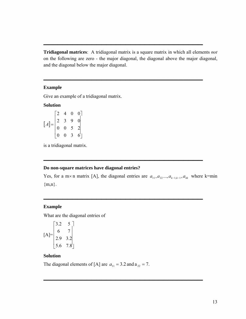
_________________________________ Tridiagonal matrices: A tridiagonal matrix is a square matrix in which all elements not on the following are zero - the major diagonal, the diagonal above the major diagonal, and the diagonal below the major diagonal.
_________________________________ Example
Give an example of a tridiagonal matrix.
Solution
[ ]⎥⎥⎥⎥
⎦
⎤
⎢⎢⎢⎢
⎣
⎡
=
6300250009320042
A
is a tridiagonal matrix.
_________________________________ Do non-square matrices have diagonal entries?
Yes, for a m×n matrix [A], the diagonal entries are where k=min
{m,n}. kkkk aaaa ,...,, 1,12211 −−
_________________________________ Example
What are the diagonal entries of
[A]=
⎥⎥⎥⎥
⎦
⎤
⎢⎢⎢⎢
⎣
⎡
8.76.52.39.2
7652.3
Solution
The diagonal elements of [A] are .7a and 2.3 2211 ==a
_________________________________
13

Diagonally Dominant Matrix: A n×n square matrix [A] is a diagonally dominant matrix if
∑≠=
≥n
jij
ijii aa1
|| for all i =1, 2, …, n
and ∑≠=
>n
jij
ijii aa1
|| for at least one i,
that is, for each row, the absolute value of the diagonal element is greater than or equal to the sum of the absolute values of the rest of the elements of that row, and that the inequality is strictly greater than for at least one row. Diagonally dominant matrices are important in ensuring convergence in iterative schemes of solving simultaneous linear equations.
_________________________________ Example
Give examples of diagonally dominant matrices and not diagonally dominant matrices.
Solution
[ ]⎥⎥⎥
⎦
⎤
⎢⎢⎢
⎣
⎡−−=623242
7615A
is a diagonally dominant matrix
as
13761515 131211 =+=+≥== aaa
42244 232122 =+=+≥=−= aaa
52366 323133 =+=+≥== aaa
and for at least one row, that is Rows 1 and 3 in this case, the inequality is a strictly greater than inequality.
[ ]⎥⎥⎥
⎦
⎤
⎢⎢⎢
⎣
⎡
−−
−=
001.5232429615
A
14
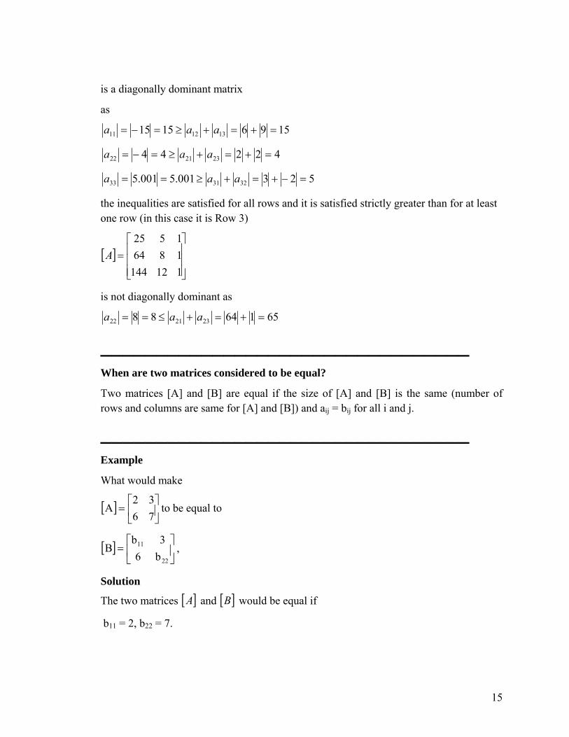
is a diagonally dominant matrix
as
15961515 131211 =+=+≥=−= aaa
42244 232122 =+=+≥=−= aaa
523001.5001.5 323133 =−+=+≥== aaa
the inequalities are satisfied for all rows and it is satisfied strictly greater than for at least one row (in this case it is Row 3)
[ ]⎥⎥⎥
⎦
⎤
⎢⎢⎢
⎣
⎡=
11214418641525
A
is not diagonally dominant as
6516488 232122 =+=+≤== aaa
_________________________________ When are two matrices considered to be equal?
Two matrices [A] and [B] are equal if the size of [A] and [B] is the same (number of rows and columns are same for [A] and [B]) and aij = bij for all i and j.
_________________________________ Example
What would make
[ ] ⎥⎦
⎤⎢⎣
⎡=
7632
A to be equal to
[ ] ⎥⎦
⎤⎢⎣
⎡=
22
11
b63b
B ,
Solution
The two matrices [ and [ would be equal if ]A ]B
b11 = 2, b22 = 7.
15

Key Terms
Matrix Vector Sub-matrix Square matrix
Upper triangular matrix Lower triangular matrix Diagonal matrix
Identity matrix Zero matrix Tridiagonal matrix
Diagonally dominant matrix Equal matrices.
Homework Assignment 1. Write an example of a row vector of dimension 4.
Answer: [ ] 3265 2. Write an example of a column vector of dimension 4.
Answer:
⎥⎥⎥⎥
⎦
⎤
⎢⎢⎢⎢
⎣
⎡−
5.237
5
3. Write an example of a square matrix of order 4×4.
Answer:
⎥⎥⎥⎥
⎦
⎤
⎢⎢⎢⎢
⎣
⎡−
−
4321.18765.115323209
Write an example of a tridiagonal matrix of order 4×4. Answer:
⎥⎥⎥⎥
⎦
⎤
⎢⎢⎢⎢
⎣
⎡
−1.41.2005.332.60
02.221.20036
4.
16

Write an example of a identity matrix of order 5×5.5.
Answer:
⎥⎥⎥⎥⎥⎥
⎦
⎤
⎢⎢⎢⎢⎢⎢
⎣
⎡
1000001000001000001000001
6. Write an example of a upper triangular matrix of order 4×4.
Answer:
⎥⎥⎥⎥
⎦
⎤
⎢⎢⎢⎢
⎣
⎡
6000540032109326
Write an example of a lower triangular matrix of order 4×4.
Answer:
⎥⎥⎥⎥
⎦
⎤
⎢⎢⎢⎢
⎣
⎡
6535042400130002
7.
8. Are these matrices strictly diagonally dominant?
a) [ ] ⎥⎥⎥
⎦
⎤
⎢⎢⎢
⎣
⎡−=
6232427615
A
b) [ ]⎥⎥⎥
⎦
⎤
⎢⎢⎢
⎣
⎡
−−=
523242765
A
17

c) [ ] ⎥⎥⎥
⎦
⎤
⎢⎢⎢
⎣
⎡
−−=
1257286235
A
Answer: a) Yes b) No c)No
9. .Find all the submatrices of
⎥⎦
⎤⎢⎣
⎡−−
=6001.000710
][A
Answer: , [ ], [ , [ ]10 7− ]0 [ ]0 , [ ]001.0− , [ ]6
, , , ⎥⎦
⎤⎢⎣
⎡0
10⎥⎦
⎤⎢⎣
⎡−−001.7
⎥⎦
⎤⎢⎣
⎡60 [ ]0710 − ,
[ ]6001.00 − , , ⎥⎦
⎤⎢⎣
⎡−−
001.00710
, , [10,-7], [10,0], [-7,0], [0,6],⎥⎦
⎤⎢⎣
⎡60010
⎥⎦
⎤⎢⎣
⎡−−
6001.007
[0,-0.001],[-0.001,6]
If ⎥⎦
⎤⎢⎣
⎡ −=
2014
[A]10.
What are b11 and b12 in
⎥⎦
⎤⎢⎣
⎡=
40b
[B] 1211 b
if [B] = 2[A].
Answers: 8, -2
18
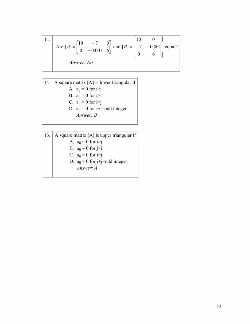
Are and equal? ⎥⎦
⎤⎢⎣
⎡−−
=6001.000710
][A⎥⎥⎥
⎦
⎤
⎢⎢⎢
⎣
⎡−−=
60001.07
010][B
11.
Answer: No
A square matrix [A] is lower triangular if
A. aij = 0 for i>j B. aij = 0 for j>i C. aij = 0 for i=j D. aij = 0 for i+j=odd integer
Answer: B
12.
13. A square matrix [A] is upper triangular if
A. aij = 0 for i>j B. aij = 0 for j>i C. aij = 0 for i=j D. aij = 0 for i+j=odd integer Answer: A
19

Chapter 2 Vectors _________________________________ After reading this chapter, you should be able to
Know what a vector is
How to add and subtract vectors
How to find linear combination of vectors and their relationship to a set of equations
Know what it means to have linearly independent set of vectors
How to find the rank of a set of vectors
_______________________________ What is a vector?
A vector is a collection of numbers in a definite order. If it is a collection of ‘n’ numbers, it is called a n-dimensional vector. So the vector A
r given by
⎥⎥⎥⎥
⎦
⎤
⎢⎢⎢⎢
⎣
⎡
=
na
aa
AM
r 2
1
is a n-dimensional column vector with n components, a1, a2 ,. . . , an. The above is a column vector. A row vector [B] is of the form
Br
= [b1, b2,. . . , bn]
where Br
is a n-dimensional row vector with n components b1, b2, . . ., bn.
_________________________________ Example
Give an example of a 3-dimensional column vector.
Solution
20
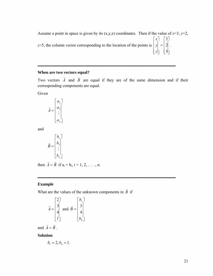
Assume a point in space is given by its (x,y,z) coordinates. Then if the value of x=3, y=2,
z=5, the column vector corresponding to the location of the points is . ⎥⎥⎥
⎦
⎤
⎢⎢⎢
⎣
⎡=
⎥⎥⎥
⎦
⎤
⎢⎢⎢
⎣
⎡
523
zyx
_________________________________ When are two vectors equal?
Two vectors Ar
and Br
are equal if they are of the same dimension and if their corresponding components are equal.
Given
⎥⎥⎥⎥
⎦
⎤
⎢⎢⎢⎢
⎣
⎡
=
na
aa
AM
r 2
1
and
⎥⎥⎥⎥
⎦
⎤
⎢⎢⎢⎢
⎣
⎡
=
nb
bb
BM
r 2
1
then BArr
= if ai = bi, i = 1, 2, . . . ., n.
_________________________________ Example
What are the values of the unknown components in Br
if
and
⎥⎥⎥⎥
⎦
⎤
⎢⎢⎢⎢
⎣
⎡
=
1432
Ar
⎥⎥⎥⎥
⎦
⎤
⎢⎢⎢⎢
⎣
⎡
=
4
1
43
b
b
Br
and BArr
= .
Solution
1 ,2 41 == bb .
21

How do you add two vectors?
Two vectors can be added only if they are of the same dimension and the addition is given by
[ ] [ ]⎥⎥⎥⎥
⎦
⎤
⎢⎢⎢⎢
⎣
⎡
+
⎥⎥⎥⎥
⎦
⎤
⎢⎢⎢⎢
⎣
⎡
=+
nn b
bb
a
aa
BAMM2
1
2
1
⎥⎥⎥⎥
⎦
⎤
⎢⎢⎢⎢
⎣
⎡
+
++
=
nn ba
baba
M22
11
_________________________________ Example
Add the two vectors
and
⎥⎥⎥⎥
⎦
⎤
⎢⎢⎢⎢
⎣
⎡
=
1432
Ar
⎥⎥⎥⎥
⎦
⎤
⎢⎢⎢⎢
⎣
⎡−
=
732
5
Br
Solution
⎥⎥⎥⎥
⎦
⎤
⎢⎢⎢⎢
⎣
⎡−
+
⎥⎥⎥⎥
⎦
⎤
⎢⎢⎢⎢
⎣
⎡
=+
732
5
1432
BArr
⎥⎥⎥⎥
⎦
⎤
⎢⎢⎢⎢
⎣
⎡
++−+
=
71342352
22

⎥⎥⎥⎥
⎦
⎤
⎢⎢⎢⎢
⎣
⎡
=
8717
_________________________________ Example
A store sells three brands of tires, Tirestone, Michigan and Cooper. In quarter 1, the sales are given by the vector
⎥⎥⎥
⎦
⎤
⎢⎢⎢
⎣
⎡=
6525
1Ar
where the rows represent the three brands of tires sold – Tirestone, Michigan and Cooper. In quarter 2, the sales are given by
⎥⎥⎥
⎦
⎤
⎢⎢⎢
⎣
⎡=
61020
2Ar
What is the total sale of each brand of tire in the first half year?
Solution
The total sales would be given by
21 AACrrr
+=
⎥⎥⎥
⎦
⎤
⎢⎢⎢
⎣
⎡+
⎥⎥⎥
⎦
⎤
⎢⎢⎢
⎣
⎡=
61020
6525
⎥⎥⎥
⎦
⎤
⎢⎢⎢
⎣
⎡
+++
=66
1052025
⎥⎥⎥
⎦
⎤
⎢⎢⎢
⎣
⎡=
121545
23
So number of Tirestone tires sold is 45, Michigan is 15 and Cooper is 12 in the first half year.
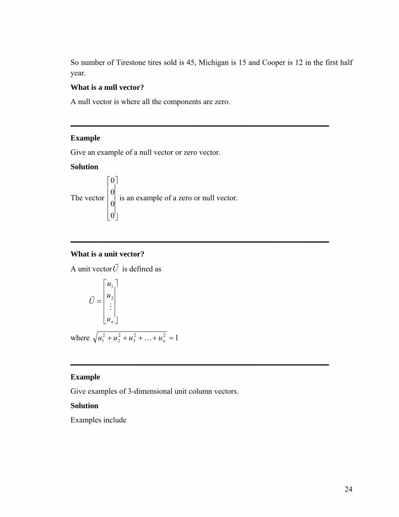
What is a null vector?
A null vector is where all the components are zero.
_________________________________ Example
Give an example of a null vector or zero vector.
Solution
The vector is an example of a zero or null vector.
⎥⎥⎥⎥
⎦
⎤
⎢⎢⎢⎢
⎣
⎡
0000
_________________________________ What is a unit vector?
A unit vectorUr
is defined as
⎥⎥⎥⎥
⎦
⎤
⎢⎢⎢⎢
⎣
⎡
=
nu
uu
UM
r 2
1
where 1223
22
21 =++++ nuuuu K
_________________________________ Example
Give examples of 3-dimensional unit column vectors.
Solution
Examples include
24
,010
,
02
12
1
,001
,
313
13
1
⎥⎥⎥
⎦
⎤
⎢⎢⎢
⎣
⎡
⎥⎥⎥⎥⎥⎥
⎦
⎤
⎢⎢⎢⎢⎢⎢
⎣
⎡
⎥⎥⎥
⎦
⎤
⎢⎢⎢
⎣
⎡
⎥⎥⎥⎥⎥⎥
⎦
⎤
⎢⎢⎢⎢⎢⎢
⎣
⎡
etc.
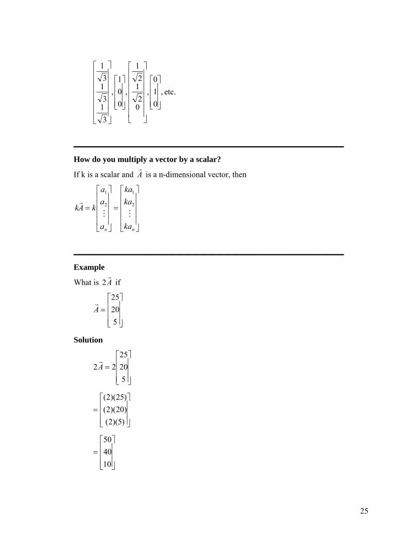
_________________________________ How do you multiply a vector by a scalar?
If k is a scalar and Ar
is a n-dimensional vector, then
⎥⎥⎥⎥
⎦
⎤
⎢⎢⎢⎢
⎣
⎡
=
⎥⎥⎥⎥
⎦
⎤
⎢⎢⎢⎢
⎣
⎡
=
nn ka
kaka
a
aa
kAkMM
r 2
1
2
1
_________________________________ Example
What is Ar
2 if
⎥⎥⎥
⎦
⎤
⎢⎢⎢
⎣
⎡=
52025
Ar
Solution
⎥⎥⎥
⎦
⎤
⎢⎢⎢
⎣
⎡=
52025
22Ar
⎥⎥⎥
⎦
⎤
⎢⎢⎢
⎣
⎡=
)5)(2()20)(2()25)(2(
⎥⎥⎥
⎦
⎤
⎢⎢⎢
⎣
⎡=
104050
25
_________________________________ Example
A store sells three brands of tires, Tirestone, Michigan and Cooper. In quarter 1, the sales are given by the vector
⎥⎥⎥
⎦
⎤
⎢⎢⎢
⎣
⎡=
62525
Ar
If the goal is to increase the sales of all tires by at least 25% in the next quarter, how many of each brand should be the goal of the store?
Solution
Since the goal is to increase the sales by 25%, one would multiply the Ar
vector by 1.25,
⎥⎥⎥
⎦
⎤
⎢⎢⎢
⎣
⎡=
62525
25.1Br
⎥⎥⎥
⎦
⎤
⎢⎢⎢
⎣
⎡=
5.725.3125.31
Since the number of tires is an integer we can say that the goal of sales would be
⎥⎥⎥
⎦
⎤
⎢⎢⎢
⎣
⎡=
83232
Br
What do you mean by a linear combination of vectors?
Given 1Ar
, 2Ar
, ………. , mAr
as m vectors of same dimension n, then if k1, k2, ……. , km are scalars, then
k1 1Ar
+ k2 2Ar
+ . . …………. + km mAr
is a linear combination of the m vectors.
_________________________________ Example
26

Find the linear combinations
a) [A] – [B], and
b) [A] + [B] – 3[C], where
⎥⎥⎥
⎦
⎤
⎢⎢⎢
⎣
⎡=
⎥⎥⎥
⎦
⎤
⎢⎢⎢
⎣
⎡=
⎥⎥⎥
⎦
⎤
⎢⎢⎢
⎣
⎡=
21
10,
211
,632
CBArrr
Solution
a) ⎥⎥⎥
⎦
⎤
⎢⎢⎢
⎣
⎡−
⎥⎥⎥
⎦
⎤
⎢⎢⎢
⎣
⎡=−
211
632
BArr
⎥⎥⎥
⎦
⎤
⎢⎢⎢
⎣
⎡
−−−
=261312
⎥⎥⎥
⎦
⎤
⎢⎢⎢
⎣
⎡=
421
b) ⎥⎥⎥
⎦
⎤
⎢⎢⎢
⎣
⎡−
⎥⎥⎥
⎦
⎤
⎢⎢⎢
⎣
⎡+
⎥⎥⎥
⎦
⎤
⎢⎢⎢
⎣
⎡=−+
21
103
211
632
3CBArrr
⎥⎥⎥
⎦
⎤
⎢⎢⎢
⎣
⎡
−+−+−+
=6263133012
⎥⎥⎥
⎦
⎤
⎢⎢⎢
⎣
⎡−=
2127
_________________________________ What do you mean by vectors being linearly independent?
A set of vectors mAAAr
Krr
,,, 21 are considered to be linearly independent if
27
k1 1Ar
+ k2 2Ar
+ . ………… . + km mAr
= 0r
has only one solution of k1 = k2 = …. = km= 0.
_________________________________ Example
Are the three vectors
⎥⎥⎥
⎦
⎤
⎢⎢⎢
⎣
⎡=
⎥⎥⎥
⎦
⎤
⎢⎢⎢
⎣
⎡=
⎥⎥⎥
⎦
⎤
⎢⎢⎢
⎣
⎡=
111
,1285
,1446425
321 AAArrr
linearly independent?
Solution
Writing the linear combination of the three vectors
⎥⎥⎥
⎦
⎤
⎢⎢⎢
⎣
⎡=
⎥⎥⎥
⎦
⎤
⎢⎢⎢
⎣
⎡+
⎥⎥⎥
⎦
⎤
⎢⎢⎢
⎣
⎡+
⎥⎥⎥
⎦
⎤
⎢⎢⎢
⎣
⎡
000
111
1285
1446425
321 kkk
gives
⎥⎥⎥
⎦
⎤
⎢⎢⎢
⎣
⎡=
⎥⎥⎥
⎦
⎤
⎢⎢⎢
⎣
⎡
++++++
000
12144864525
321
321
321
kkkkkkkkk
The above equations has only one solution, k1 = k2 = k3 = 0. But how do we show that this is the only solution? This is shown below.
The above equations are 0 (1) 525 321 =++ kkk
0 (2) 864 321 =++ kkk
0 (3) 12144 321 =++ kkk
Subtracting eqn (1) from eqn (2) gives
0339 21 =+ kk
(4) 12 13kk −=
Multiplying eqn (1) by 8 and subtracting it from eqn (2) that is first multiplied by 5 gives
28

03120 31 =− kk
(5) 13 40kk =
Remember we found eqn (4) and eqn (5) just from eqns (1) and (2).
Substitution of eqn (4) and (5) in eqn (3) for and gives 1k 2k
040)13(12144 111 =+−+ kkk
028 1 =k
01 =kThis means that k1 has to be zero, and coupled with equations (4) and (5), k2 and k3 are also zero. So the only solution is k1 = k2 = k3 = 0. The three vectors hence are linearly independent.
_________________________________ Example
Are the three vectors
⎥⎥⎥
⎦
⎤
⎢⎢⎢
⎣
⎡=
⎥⎥⎥
⎦
⎤
⎢⎢⎢
⎣
⎡=
⎥⎥⎥
⎦
⎤
⎢⎢⎢
⎣
⎡=
24146
,752
,521
321 AAArr
linearly independent?
Solution
By inspection,
213 22 AAArrr
+=
or
022 321 =+−− AAArrr
So the linear combination
0332211
rrrr=++ AkAkAk
has a non-zero solution
1,2,2 321 =−=−= kkk
Hence the set of vectors is linearly dependent.
29
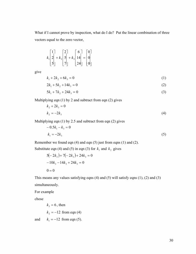
What if I cannot prove by inspection, what do I do? Put the linear combination of three
vectors equal to the zero vector,
⎥⎥⎥
⎦
⎤
⎢⎢⎢
⎣
⎡=
⎥⎥⎥
⎦
⎤
⎢⎢⎢
⎣
⎡+
⎥⎥⎥
⎦
⎤
⎢⎢⎢
⎣
⎡+
⎥⎥⎥
⎦
⎤
⎢⎢⎢
⎣
⎡
000
24146
752
521
321 kkk
give 0 (1) 62 321 =++ kkk
0 (2) 1452 321 =++ kkk
0 (3) 2475 321 =++ kkk
Multiplying eqn (1) by 2 and subtract from eqn (2) gives 0
0
2 32 =+ kk
(4) 32 2kk −=
Multiplying eqn (1) by 2.5 and subtract from eqn (2) gives 5.0 31 =−− kk
(5) 31 2kk −=
Remember we found eqn (4) and eqn (5) just from eqns (1) and (2). Substitute eqn (4) and (5) in eqn (3) for and gives 1k 2k
( ) ( ) 0242725 333 =+−+− kkk
0241410 333 =+−− kkk
00 =
This means any values satisfying eqns (4) and (5) will satisfy eqns (1), (2) and (3)
simultaneously.
For example
chose , then 63 =k
from eqn (4) 122 −=k
and from eqn (5). 121 −=k
30

Hence we have nontrivial solution of [ ] [ ]61212321 −−=kkk . This implies the
three given vectors are linearly dependent. Can you find another nontrivial solution?
What about the following three vectors?
⎥⎥⎥
⎦
⎤
⎢⎢⎢
⎣
⎡
⎥⎥⎥
⎦
⎤
⎢⎢⎢
⎣
⎡
⎥⎥⎥
⎦
⎤
⎢⎢⎢
⎣
⎡
25146
,752
,521
Are they linearly dependent or linearly independent?
Note that the only difference between this set of vectors and the previous one is the third
entry in the third vector. Hence, equations (4) and (5) are still valid. What conclusion do
you draw when you plug in equations (4) and (5) in the third equation: ? What has changed? 02575 321 =++ kkk
Example
Are the three vectors
⎥⎥⎥
⎦
⎤
⎢⎢⎢
⎣
⎡=
⎥⎥⎥
⎦
⎤
⎢⎢⎢
⎣
⎡=
⎥⎥⎥
⎦
⎤
⎢⎢⎢
⎣
⎡=
211
,1385
,896425
321 AAArrr
linearly independent.
Solution
Writing the linear combination of the three vectors
⎥⎥⎥
⎦
⎤
⎢⎢⎢
⎣
⎡=
⎥⎥⎥
⎦
⎤
⎢⎢⎢
⎣
⎡+
⎥⎥⎥
⎦
⎤
⎢⎢⎢
⎣
⎡+
⎥⎥⎥
⎦
⎤
⎢⎢⎢
⎣
⎡
000
211
1385
896425
321 kkk
gives
⎥⎥⎥
⎦
⎤
⎢⎢⎢
⎣
⎡=
⎥⎥⎥
⎦
⎤
⎢⎢⎢
⎣
⎡
++++++
000
21389864525
321
321
321
kkkkkkkkk
In addition to k1 = k2 = k3 = 0, one can find other solutions for which k1, k2, k3 are not equal to zero. For example k1 = 1, k2 = -13, k3 = 40 is also a solution. This implies
31

⎥⎥⎥
⎦
⎤
⎢⎢⎢
⎣
⎡=
⎥⎥⎥
⎦
⎤
⎢⎢⎢
⎣
⎡+
⎥⎥⎥
⎦
⎤
⎢⎢⎢
⎣
⎡−
⎥⎥⎥
⎦
⎤
⎢⎢⎢
⎣
⎡
000
211
401385
13896425
1
So the linear combination that gives us a zero vector consists of non-zero constants.
Hence 321 ,, AAArrr
are linearly dependent.
_________________________________ What do you mean by the rank of a set of vectors?
From a set of n-dimensional vectors, the maximum number of linearly independent vectors in the set is called the rank of the set of vectors. Note that the rank of the vectors can never be greater than its dimension.
_________________________________ Example
What is the rank of
⎥⎥⎥
⎦
⎤
⎢⎢⎢
⎣
⎡=
⎥⎥⎥
⎦
⎤
⎢⎢⎢
⎣
⎡=
⎥⎥⎥
⎦
⎤
⎢⎢⎢
⎣
⎡=
111
,1285
,1446425
321 AAArrr
Solution:
Since we found in a previous example that ,, 21 AArr
and 3Ar
are linearly independent, the
rank of the set of vectors 321 ,, AAArrr
is 3.
_________________________________ Example
What is the rank of
⎥⎥⎥
⎦
⎤
⎢⎢⎢
⎣
⎡=
⎥⎥⎥
⎦
⎤
⎢⎢⎢
⎣
⎡=
⎥⎥⎥
⎦
⎤
⎢⎢⎢
⎣
⎡=
211
,1385
,896425
321 AAArrr
32

Solution
In an earlier example, we found that 21 , AArr
and 3Ar
are linearly dependent, the rank of
321 ,, AAArrr
is hence not 3, and is less than 3. Is it 2? Let us choose
⎥⎥⎥
⎦
⎤
⎢⎢⎢
⎣
⎡=
⎥⎥⎥
⎦
⎤
⎢⎢⎢
⎣
⎡=
1385
,896425
21 AArr
Linear combination of and 1Ar
2Ar
equal to zero has only one solution. So the rank is 2.
_________________________________ Example
What is the rank of
⎥⎥⎥
⎦
⎤
⎢⎢⎢
⎣
⎡=
⎥⎥⎥
⎦
⎤
⎢⎢⎢
⎣
⎡=
⎥⎥⎥
⎦
⎤
⎢⎢⎢
⎣
⎡=
533
,422
,211
321 AAArrr
Solution
From inspection, 12 2AAr
=→
, that implies
.002 321
rr=+−
→→
AAA Hence
.0332211
rr=++
→→
AkAkAkhas a nontrivial solution.
So 321 ,,→→
AAAr
are linearly dependent, and hence the rank of the three vectors is not 3. Since
12 2→→
= AA , are linearly dependent, 21
→→
AandAbut
.03311
rr=+
→
AkAk
has trivial solution as the only solution. So are linearly independent. The rank of the above three vectors is 2.
31
→→
AandA
___________________________
33

Prove that if a set of vectors contains the null vector, the set of vectors is linearly dependent.
Let be a set of n-dimensional vectors, then mAAAr
Krr
,,, 21
→
=+++ 02211 mm AkAkAkr
Krr
is a linear combination of the ‘m’ vectors. Then assuming if 1Ar
is the zero or null vector, any value of coupled with 1k 032 ==== mkkk K will satisfy the above equation. Hence the set of vectors is linearly dependent as more than one solution exists. Prove that if a set of vectors are linearly independent, then a subset of the m vectors also has to be linearly independent. Let this subset be
apaa AAAr
Krr
,,, 21 where p < m. Then if this subset is linearly dependent, the linear combination
→
=+++ 02211 appaa AkAkAkr
Krr
has a non-trivial solution. So
→
+ =++++++ 00.......0 )1(2211 ampaappaa AAAkAkAkrrr
Krr
has a non-trivial solution too, where are the rest of the (m-p) vectors. However, this is a contradiction. Therefore, a subset of linearly independent vectors cannot be linearly dependent.
( ) ampa AA→
+
→
,,1 K
Prove that if a set of vectors is linearly dependent, then at least one vector can be written as a linear combination of others.
Let be linearly dependent, then there exists a set of numbers mAAAr
Krr
,,, 21
mkk ,,1 K not all of which are zero for the linear combination
→
=+++ 02211 mm AkAkAkr
Krr
that one of non-zero values of miki ,,1, K= , is for let i = p, then
.11
11
22
m
p
mp
p
pp
p
p
pp A
kk
Ak
kA
kk
AkkA
→
+
→+
−
→− −−−−−−= KK
r
and that proves the theorem. Prove that if the dimension of a set of vectors is less than the number of vectors in the set, then the set of vectors is linearly dependent.
Can you prove it??
34

How can vectors be used to write simultaneous linear equations?
A set of m linear equations with n unknowns is written as
1111 1 cxaxa nn =++K
22121 cxaxa nn =++K
MM
MM
nnmnm cxaxa =++K11
where
nxxx ,,, 21 K are the unknowns, then in the vector notation they can be written as
CAxAxAx nn
rrK
rr=+++ 2211
where
⎥⎥⎥
⎦
⎤
⎢⎢⎢
⎣
⎡=
⎥⎥⎥
⎦
⎤
⎢⎢⎢
⎣
⎡=
⎥⎥⎥
⎦
⎤
⎢⎢⎢
⎣
⎡=
mn
n
n
m
m
a
aA
a
aA
a
aA
Mr
Mr
Mr
1
2
12
2
1
11
1
The problem now becomes whether you can find the scalars 1x , ………, such that the linear combination
nx
CAxAx nn
rrr=++ ..........11 .
Example
Write
8
2
2
.106525 321 =++ xxx
.177864 321 =++ xxx
.27912144 321 =++ xxx
35

as a linear combination of vectors.
Solution
⎥⎥⎥
⎦
⎤
⎢⎢⎢
⎣
⎡=
⎥⎥⎥
⎦
⎤
⎢⎢⎢
⎣
⎡
++++++
2.2792.1778.106
12144864525
321
321
321
xxxxxxxxx
⎥⎥⎥
⎦
⎤
⎢⎢⎢
⎣
⎡=
⎥⎥⎥
⎦
⎤
⎢⎢⎢
⎣
⎡+
⎥⎥⎥
⎦
⎤
⎢⎢⎢
⎣
⎡+
⎥⎥⎥
⎦
⎤
⎢⎢⎢
⎣
⎡
2.2792.1778.106
111
1285
1446425
321 xxx
What is the definition of the dot product of two vectors?
Let and [ ]naaaA ,,, 21 Kr= [ ]nbbbB ,,, 21 K
r= be two n-dimensional vectors. Then the
dot product of the two vectors Ar
and Br
is defined as
∑=
=+++=⋅n
iiinn babababaBA
12211 K
rr
A dot product is also called an inner product or scalar.
_________________________________ Example
Find the dot product of the two vectors Ar
= (4, 1, 2, 3) and Br
= (3, 1, 7, 2).
Solution
( ) ( 2,7,1,33,2,1,4 ⋅=⋅ BArr
)
= (4)(3)+(1)(1)+(2)(7)+(3)(2)
= 33
_________________________________ Example
A product line needs three types of rubber as given in the table below.
Rubber Type Weight Cost per pound
lbs $
36

A
B
C
200
250
310
20.23
30.56
29.12
How much is the total price of the rubber needed?
Solution
The weight vector is given by
( )310,250,200=Wr
and the cost vector is given by
( )12.29,56.30,23.20=Cr
.
The total cost of the rubber would be the dot product of Wr
and Cr
.
( ) ( 12.29,56.30,23.20310,250,200 ⋅=⋅CWrr
)
= (200)(20.23) + (250)(30.56) + (310)(29.12)
= 4046 + 7640 + 9027.2
= $20713.2
_________________________________ Key Terms
Vector Addition of vectors Subtraction of vectors
Unit vectors Null vector Scalar multiplication of vectors
Linear combination of vectors Linearly independent vectors
Rank Dot products.
_________________________________ Homework
1. For
37
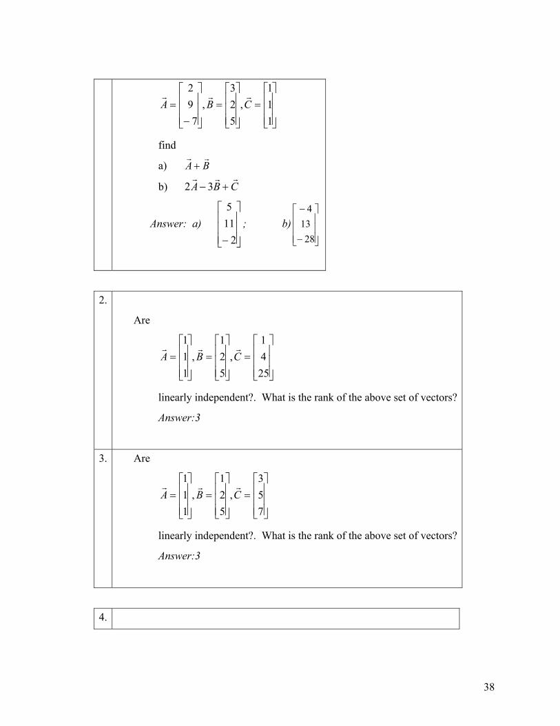
⎥⎥⎥
⎦
⎤
⎢⎢⎢
⎣
⎡=
⎥⎥⎥
⎦
⎤
⎢⎢⎢
⎣
⎡=
⎥⎥⎥
⎦
⎤
⎢⎢⎢
⎣
⎡
−=
111
,523
,7
92
CBArrr
find
a) BArr
+
b) CBArrr
+− 32
Answer: a) ; b)⎥⎥⎥
⎦
⎤
⎢⎢⎢
⎣
⎡
− 2115
⎥⎥⎥
⎦
⎤
⎢⎢⎢
⎣
⎡
−
−
2813
4
2.
Are
⎥⎥⎥
⎦
⎤
⎢⎢⎢
⎣
⎡=
⎥⎥⎥
⎦
⎤
⎢⎢⎢
⎣
⎡=
⎥⎥⎥
⎦
⎤
⎢⎢⎢
⎣
⎡=
2541
,521
,111
CBArrr
linearly independent?. What is the rank of the above set of vectors?
Answer:3
3. Are
⎥⎥⎥
⎦
⎤
⎢⎢⎢
⎣
⎡=
⎥⎥⎥
⎦
⎤
⎢⎢⎢
⎣
⎡=
⎥⎥⎥
⎦
⎤
⎢⎢⎢
⎣
⎡=
753
,521
,111
CBArrr
linearly independent?. What is the rank of the above set of vectors?
Answer:3
4.
38

Are
⎥⎥⎥
⎦
⎤
⎢⎢⎢
⎣
⎡=
⎥⎥⎥
⎦
⎤
⎢⎢⎢
⎣
⎡=
⎥⎥⎥
⎦
⎤
⎢⎢⎢
⎣
⎡=
5.52.21.1
,1042
,521
CBArrr
linearly independent? What is the rank of the above set of vectors?
Answer:1
5. If a set of vectors contains the null vector, the set of vectors is linearly
A. independent.
B. dependent.
Answer:B
6. If a set of vectors is linearly independent, a subset of the vectors is linearly
A. independent.
B. dependent.
Answer:A
7.
If a set of vectors is linearly dependent, then
A. at least one vector can be written as a linear combination of others.
B. at least one vector is a null vector.
Answer:A
8.
If the dimension of a set of vectors is less than the number of vectors in the set, then the set of vectors is linearly
39
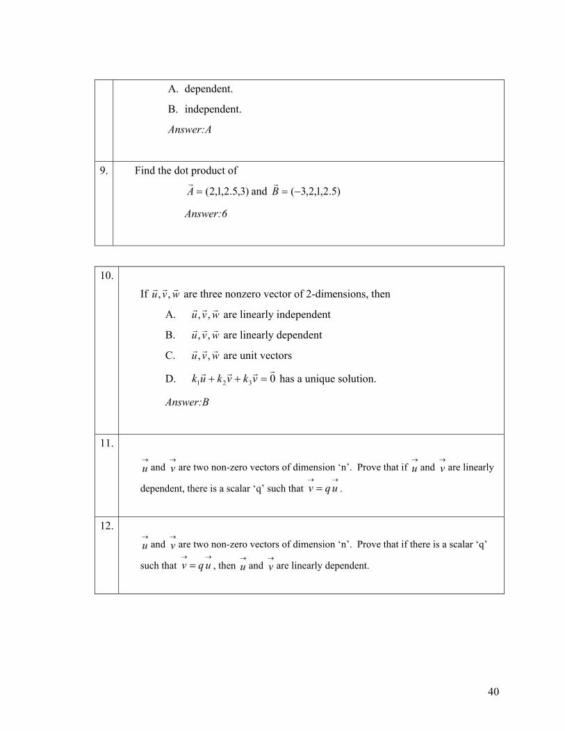
A. dependent.
B. independent.
Answer:A
9. Find the dot product of
)3,5.2,1,2(=Ar
and )5.2,1,2,3(−=Br
Answer:6
10.
If are three nonzero vector of 2-dimensions, then wvu rrr ,,
A. are linearly independent wvu rrr ,,
B. are linearly dependent wvu rrr ,,
C. are unit vectors wvu rrr ,,
D. 0321
rrrr=++ vkvkuk has a unique solution.
Answer:B
11.
u→
and are two non-zero vectors of dimension ‘n’. Prove that if and are linearly
dependent, there is a scalar ‘q’ such that .
v→
u→
v→
→→
= uqv
12.
u→
and are two non-zero vectors of dimension ‘n’. Prove that if there is a scalar ‘q’
such that , then and are linearly dependent.
v→
→→
= uqv u→
v→
40

Chapter 3 Binary Matrix Operations _________________________________ After reading this chapter, you will be able to
Add, subtract and multiply matrices
Learn rules of binary operations on matrices
________________________________ How do you add two matrices?
Two matrices [A] and [B] can be added only if they are the same size, then the addition is shown as
[C] = [A] + [B]
where
cij = aij + bij
_________________________________ Example
Add two matrices
[ ] ⎥⎦
⎤⎢⎣
⎡=
721325
A
[ ] ⎥⎦
⎤⎢⎣
⎡ −=
1953276
B
Solution
[ ] [ ] [ ]BAC +=
⎥⎦
⎤⎢⎣
⎡ −+⎥
⎦
⎤⎢⎣
⎡=
1953276
721325
41

⎥⎦
⎤⎢⎣
⎡+++−++
=1975231237265
⎥⎦
⎤⎢⎣
⎡=
26741911
_________________________________ Example
Blowout r’us store has two locations ‘A’ and ‘B’, and their sales of tires are given by make (in rows) and quarters (in columns) as shown below.
[ ]⎥⎥⎥
⎦
⎤
⎢⎢⎢
⎣
⎡=
2771662515105232025
A
[ ]⎥⎥⎥
⎦
⎤
⎢⎢⎢
⎣
⎡=
2071421156304520
B
where the rows represent sale of Tirestone, Michigan and Copper tires and the columns represent the quarter number - 1, 2, 3, 4. What are the total sales of the two locations by make and quarter?
Solution
[ ] [ ] [ ]BAC +=
= + ⎥⎥⎥
⎦
⎤
⎢⎢⎢
⎣
⎡
2771662515105232025
⎥⎥⎥
⎦
⎤
⎢⎢⎢
⎣
⎡
2071421156304520
=( ) ( ) ( ) ( )( ) ( ) ( ) ( )( ) ( ) ( ) ( ⎥
⎥⎥
⎦
⎤
⎢⎢⎢
⎣
⎡
++++++++++++
20277711646212515156103502435202025
)
⎥⎥⎥
⎦
⎤
⎢⎢⎢
⎣
⎡=
471417104630168272545
42

So if one wants to know the total number of Copper tires sold in quarter 4 in the two locations, we would look at Row 3 – Column 4 to give
.47c34 =
_________________________________ How do you subtract two matrices?
Two matrices [A] and [B] can be subtracted only if they are the same size and the subtraction is given by
[D] = [A] – [B]
where
dij = aij - bij
_________________________________ Example
Subtract matrix [B] from matrix [A].
[ ] ⎥⎦
⎤⎢⎣
⎡=
721325
A
[ ] ⎥⎦
⎤⎢⎣
⎡ −=
1953276
B
Solution
[ ] [ ] [ ]BAC −=
⎥⎦
⎤⎢⎣
⎡ −−⎥
⎦
⎤⎢⎣
⎡=
1953276
721325
⎥⎦
⎤⎢⎣
⎡−−−−−−−
=1975231
)2(37265
⎥⎦
⎤⎢⎣
⎡−−−
−−=
1232551
_________________________________
43

Example
Blowout r’us store has two locations A and B and their sales of tires are given by make (in rows) and quarters (in columns) as shown below.
[ ]⎥⎥⎥
⎦
⎤
⎢⎢⎢
⎣
⎡=
2771662515105232025
A
[ ]⎥⎥⎥
⎦
⎤
⎢⎢⎢
⎣
⎡=
2071421156304520
B
where the rows represent sale of Tirestone, Michigan and Copper tires and the columns represent the quarter number- 1, 2, 3, 4. How many more tires did store A sell than store B of each brand in each quarter?
Solution
[D]
= [ ] [ ]BA −
= ⎥⎥⎥
⎦
⎤
⎢⎢⎢
⎣
⎡−
⎥⎥⎥
⎦
⎤
⎢⎢⎢
⎣
⎡
2071421156304520
2771662515105232025
⎥⎥⎥
⎦
⎤
⎢⎢⎢
⎣
⎡
−−−−−−−−−−−−
=20277711646212515156103502435202025
⎥⎥⎥
⎦
⎤
⎢⎢⎢
⎣
⎡ −=
70152404221155
So if you want to know how many more Copper Tires were sold in quarter 4 in Store A than Store B, d34 = 7. Note that 113 −=d implies that store A sold 1 less Michigan tire than Store B in quarter 3.
_________________________________ How do I multiply two matrices?
44
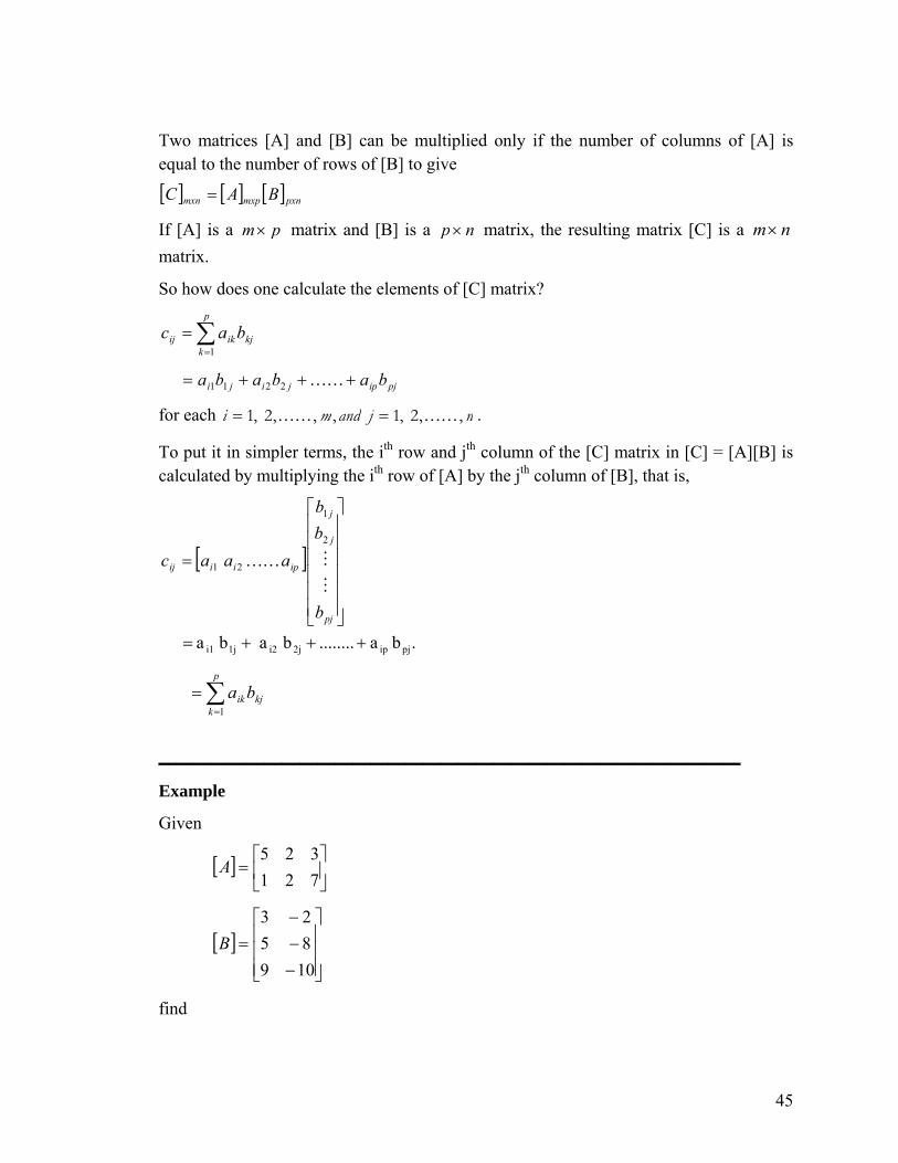
Two matrices [A] and [B] can be multiplied only if the number of columns of [A] is equal to the number of rows of [B] to give
[ ] [ ] [ ]pxnmxpmxn BAC =
If [A] is a pm× matrix and [B] is a np× matrix, the resulting matrix [C] is a nm× matrix.
So how does one calculate the elements of [C] matrix?
∑=
=p
kkjikij bac
1
pjipjiji bababa +++= KK2211
for each njandmi ,,2,1, ,,2 ,1 KKKK == .
To put it in simpler terms, the ith row and jth column of the [C] matrix in [C] = [A][B] is calculated by multiplying the ith row of [A] by the jth column of [B], that is,
[ ]
.ba ........ b a b a pj ip2ji21ji1
2
1
21
+++=
⎥⎥⎥⎥⎥⎥
⎦
⎤
⎢⎢⎢⎢⎢⎢
⎣
⎡
=
pj
j
j
ipiiij
b
bb
aaacM
MKK
∑=
=p
kkjik ba
1
_________________________________ Example
Given
[ ] ⎥⎦
⎤⎢⎣
⎡=
721325
A
[ ]⎥⎥⎥
⎦
⎤
⎢⎢⎢
⎣
⎡
−−−
=1098523
B
find
45

[ ] [ ][ ]BAC =
Solution
c12 can be found by multiplying the first row of [A] by the second column of [B],
[ ]⎥⎥⎥
⎦
⎤
⎢⎢⎢
⎣
⎡
−−−
=1082
32512c
= (5)(-2) + (2)(-8) + (3)(-10)
= -56
Similarly, one can find the other elements of [C] to give
[ ] ⎥⎦
⎤⎢⎣
⎡−−
=88765652
C
_________________________________ Example
Blowout r’us store location A and the sales of tires are given by make (in rows) and quarters (in columns) as shown below
[ ]⎥⎥⎥
⎦
⎤
⎢⎢⎢
⎣
⎡=
2771662515105232025
A
where the rows represent sale of Tirestone, Michigan and Copper tires and the columns represent the quarter number - 1, 2, 3, 4. Find the per quarter sales of store A if following are the prices of each tire.
Tirestone = $33.25
Michigan = $40.19
Copper = $25.03
Solution
The answer is given by multiplying the price matrix by the quantity sales of store A. The price matrix is , then the per quarter sales of store A would be given by
[ 03.2519.4025.33 ]
46
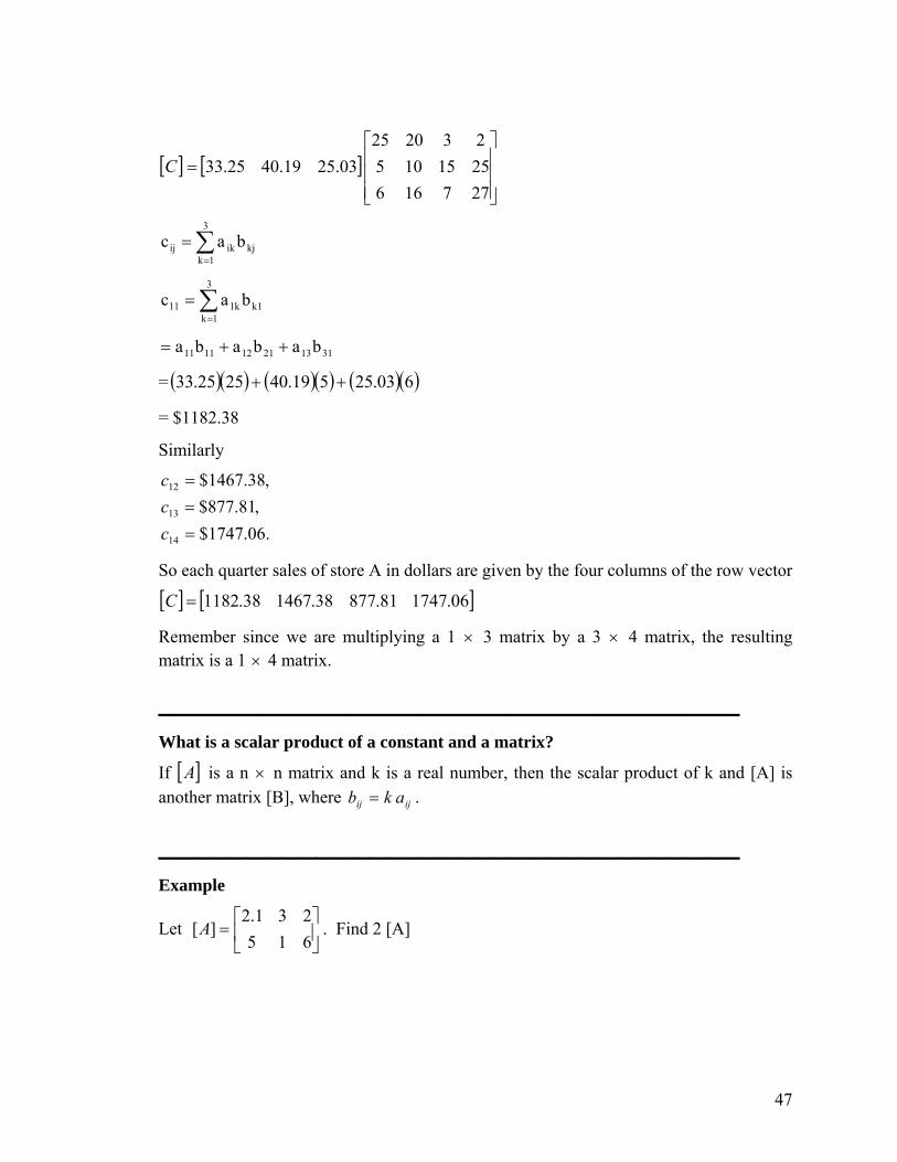
[ ]C [ ]⎥⎥⎥
⎦
⎤
⎢⎢⎢
⎣
⎡=
2771662515105232025
03.2519.4025.33
∑=
=3
1kkjikij bac
∑=
=3
1k1kk111 bac
311321121111 bababa ++=
= ( )( ) ( )( ) ( )( )603.25519.402525.33 ++
= $1182.38
Similarly
.06.1747$,81.877$
,38.1467$
14
13
12
===
ccc
So each quarter sales of store A in dollars are given by the four columns of the row vector
[ ] [ ]06.174781.87738.146738.1182=C
Remember since we are multiplying a 1 × 3 matrix by a 3 × 4 matrix, the resulting matrix is a 1 × 4 matrix.
_________________________________ What is a scalar product of a constant and a matrix?
If is a n × n matrix and k is a real number, then the scalar product of k and [A] is another matrix [B], where
[ ]Aijij akb = .
_________________________________ Example
Let . Find 2 [A] ⎥⎦
⎤⎢⎣
⎡=
615231.2
][A
47

Solution
⎥⎦
⎤⎢⎣
⎡=
615231.2
][A
Then
][2 A
=2 ⎥⎦
⎤⎢⎣
⎡615231.2
= ⎥⎦
⎤⎢⎣
⎡)6)(2()1)(2()5)(2()2)(2()3)(2()1.2)(2(
⎥⎦
⎤⎢⎣
⎡=
12210462.4
_________________________________ What is a linear combination of matrices?
If [A1], [A2], ……, [Ap] are matrices of the same size and k1, k2, ……., kp are scalars, then
[ ] [ ] [ ]pp AkAkAk +++ ........2211
is called a linear combination of [ ] [ ] [ ]., , 21 pAAA LL
_________________________________ Example
If
[ ] [ ] [ ] ⎥⎦
⎤⎢⎣
⎡=⎥
⎦
⎤⎢⎣
⎡=⎥
⎦
⎤⎢⎣
⎡=
65.3322.20
,615231.2
,123265
321 AAA
then find
[ ] [ ] [ 321 5.02 AAA −+ ]
Solution
⎥⎦
⎤⎢⎣
⎡−⎥
⎦
⎤⎢⎣
⎡+⎥
⎦
⎤⎢⎣
⎡=
65.3322.20
5.0615231.2
2123265
48
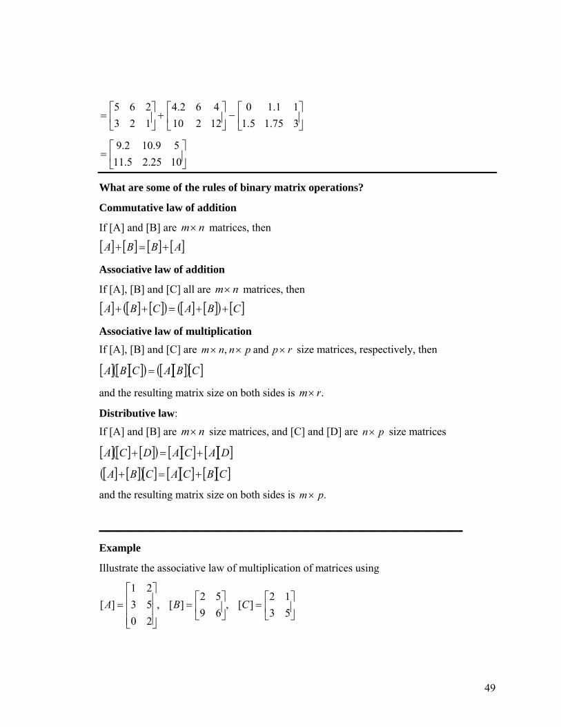
⎥⎦
⎤⎢⎣
⎡−⎥
⎦
⎤⎢⎣
⎡+⎥
⎦
⎤⎢⎣
⎡=
375.15.111.10
12210462.4
123265
⎥⎦
⎤⎢⎣
⎡=
1025.25.1159.102.9
What are some of the rules of binary matrix operations?
Commutative law of addition
If [A] and [B] are matrices, then nm×
[ ] [ ] [ ] [ ]ABBA +=+
Associative law of addition
If [A], [B] and [C] all are matrices, then nm×
[ ] [ ] [ ]( ) [ ] [ ]( ) [ ]CBACBA ++=++
Associative law of multiplication
If [A], [B] and [C] are rppnnm ××× and , size matrices, respectively, then
[ ] [ ][ ]( ) [ ][ ]( )[ ]CBACBA =
and the resulting matrix size on both sides is .rm×
Distributive law:
If [A] and [B] are size matrices, and [C] and [D] are nm× pn× size matrices
[ ] [ ] [ ]( ) [ ][ ] [ ][ ]DACADCA +=+
[ ] [ ]( )[ ] [ ][ ] [ ][ ]CBCACBA +=+
and the resulting matrix size on both sides is .pm×
_________________________________ Example
Illustrate the associative law of multiplication of matrices using
⎥⎦
⎤⎢⎣
⎡=⎥
⎦
⎤⎢⎣
⎡=
⎥⎥⎥
⎦
⎤
⎢⎢⎢
⎣
⎡=
5312
][,6952
][,205321
][ CBA
49
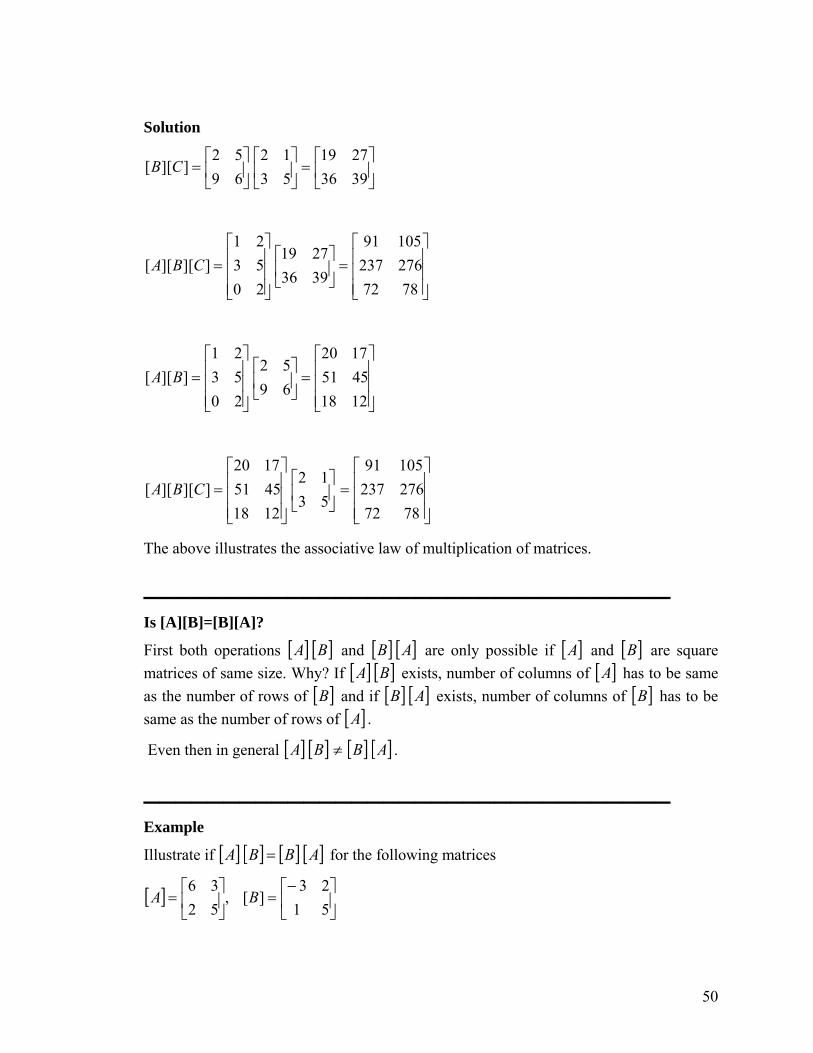
Solution
⎥⎦
⎤⎢⎣
⎡=⎥
⎦
⎤⎢⎣
⎡⎥⎦
⎤⎢⎣
⎡=
39362719
5312
6952
]][[ CB
⎥⎥⎥
⎦
⎤
⎢⎢⎢
⎣
⎡=⎥
⎦
⎤⎢⎣
⎡
⎥⎥⎥
⎦
⎤
⎢⎢⎢
⎣
⎡=
787227623710591
39362719
205321
]][][[ CBA
⎥⎥⎥
⎦
⎤
⎢⎢⎢
⎣
⎡=⎥
⎦
⎤⎢⎣
⎡
⎥⎥⎥
⎦
⎤
⎢⎢⎢
⎣
⎡=
121845511720
6952
205321
]][[ BA
⎥⎥⎥
⎦
⎤
⎢⎢⎢
⎣
⎡=
787227623710591
⎥⎦
⎤⎢⎣
⎡
⎥⎥⎥
⎦
⎤
⎢⎢⎢
⎣
⎡=
5312
121845511720
]][][[ CBA
The above illustrates the associative law of multiplication of matrices.
_________________________________ Is [A][B]=[B][A]?
First both operations and [ ]A [ ]B [ ]B [ ]A are only possible if [ ]A and [ are square matrices of same size. Why? If
]B[ ]A [ ]B exists, number of columns of has to be same
as the number of rows of and if [ ]A
[ ]B [ ]B [ ]A exists, number of columns of [ has to be same as the number of rows of
]B[ ]A .
Even then in general [ ]A [ ]B ≠ [ ]B [ ]A .
_________________________________ Example
Illustrate if [ ]A [ ] =B [ ]B [ ]A for the following matrices
[ ] ⎥⎦
⎤⎢⎣
⎡−=⎥
⎦
⎤⎢⎣
⎡=
5123
][,5236
BA
50

Solution ]][[ BA
⎥⎦
⎤⎢⎣
⎡−⎥⎦
⎤⎢⎣
⎡=
5123
5236
⎥⎦
⎤⎢⎣
⎡−−
2912715
=]][[ AB
⎥⎦
⎤⎢⎣
⎡⎥⎦
⎤⎢⎣
⎡−5236
5123
⎥⎦
⎤⎢⎣
⎡−=
2816114
[A][B] ≠ [B][A]
_________________________________ Key Terms
Addition of matrices Subtraction of matrices Multiplication of matrices
Scalar product of matrices Linear combination of matrices
Rules of binary matrix operation.
_________________________________ Homework
1. For the following matrices
⎥⎥
⎦
⎤
⎢⎢
⎣
⎡−=
1120
13
[A] , , ⎥⎦
⎤⎢⎣
⎡ −=
2014
[B]⎥⎥
⎦
⎤
⎢⎢
⎣
⎡=
7652
35
[C]
find where possible
a) 4[A] + 5[C]
b) [A][B]
c) [A] – 2[C]
51
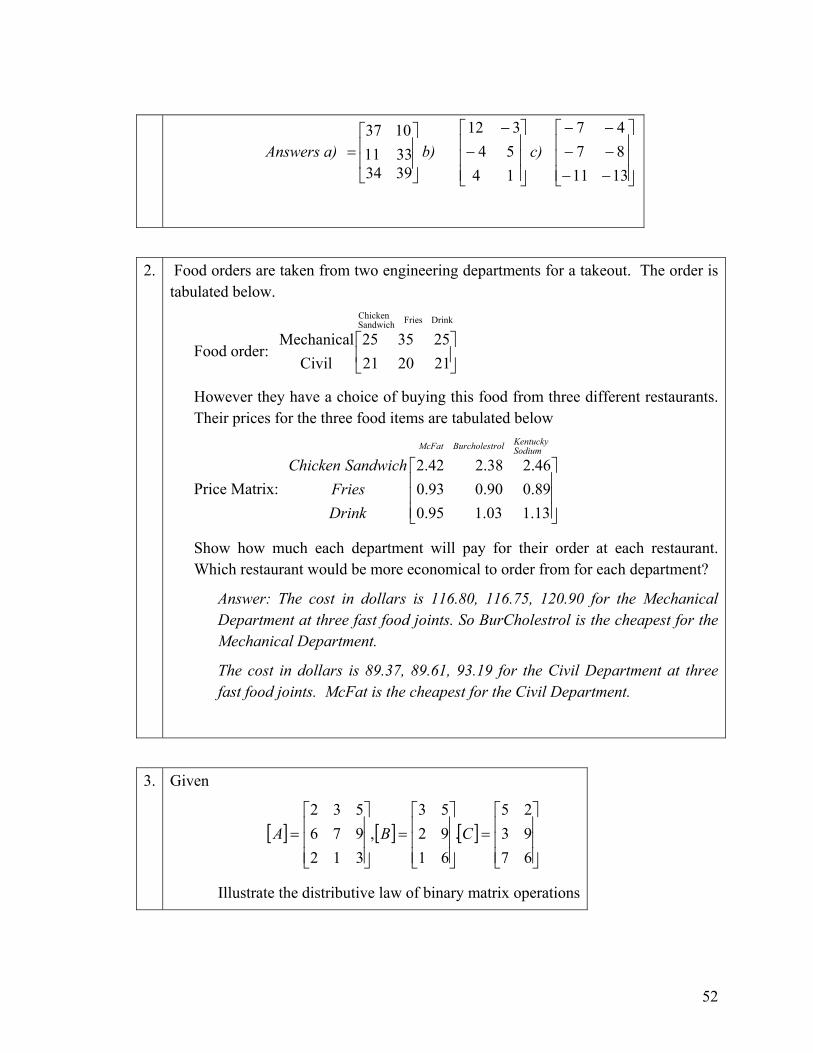
Answers a) b) c) ⎥⎥
⎦
⎤
⎢⎢
⎣
⎡=
39343310
1137
⎥⎥⎥
⎦
⎤
⎢⎢⎢
⎣
⎡−
−
1454312
⎥⎥⎥
⎦
⎤
⎢⎢⎢
⎣
⎡
−−−−−−
13118747
2. Food orders are taken from two engineering departments for a takeout. The order is tabulated below.
Food order:
DrinkFriesSandwichChicken
212021253525
CivilMechanical
⎥⎦
⎤⎢⎣
⎡
However they have a choice of buying this food from three different restaurants. Their prices for the three food items are tabulated below
Price Matrix:
SodiumKentuckyrolBurcholestMcFat
DrinkFries
SandwichChicken
⎥⎥⎥
⎦
⎤
⎢⎢⎢
⎣
⎡
13.103.195.089.090.093.046.238.242.2
Show how much each department will pay for their order at each restaurant. Which restaurant would be more economical to order from for each department?
Answer: The cost in dollars is 116.80, 116.75, 120.90 for the Mechanical Department at three fast food joints. So BurCholestrol is the cheapest for the Mechanical Department.
The cost in dollars is 89.37, 89.61, 93.19 for the Civil Department at three fast food joints. McFat is the cheapest for the Civil Department.
3. Given
[ ] [ ] [ ]⎥⎥⎥
⎦
⎤
⎢⎢⎢
⎣
⎡=
⎥⎥⎥
⎦
⎤
⎢⎢⎢
⎣
⎡=
⎥⎥⎥
⎦
⎤
⎢⎢⎢
⎣
⎡=
679325
.619253
,312976532
CBA
Illustrate the distributive law of binary matrix operations
52

[ ] [ ] [ ]( ) [ ][ ] [ ][ ]CABACBA +=+ .
4.
Let [I] be a n × n identity matrix. Show that [A][I] = [I][A] = [A] for every n × n matrix [A].
Let [ ] [ ] [ ] nnnnnn IAC ××× =
Hint: pj
n
pipij iac ∑=
=1
( ) ( ) njinjjjijjijjjjiji iaiaiaiaia ++++++= ++−− KKKK 11,11,11
Since 0=iji for ji ≠ for 1= ji = ijij ac = So [ ] [ ][ ]IAA = Similarly do the other case [ ][ ] [ ]AAI = . JUST DO IT!
5.
Consider there are only two computer companies in a country. The companies are named “Dude” and “Imac”. Each year, company Dude keeps 1/5th of its customers, while the rest switch to Imac. Each year, Imac keeps 1/3rd of its customers, while the rest switch to Dude. If in 2002, Dude has 1/6th of the market and Imac has 5/6th of the market,
a) what is the distribution of the customers between the two companies in 2003. Write the answer first as multiplication of two matrices.
b) what would be distribution when the market becomes stable? Answer: a) [ ]4111.05889.0 b) Stable distribution is [10/22 12/22] (Try to do this part of the problem by finding the distribution five years from now).
6. Given
53

, ⎥⎥⎥
⎦
⎤
⎢⎢⎢
⎣
⎡
−−−−
−=
3.123.113.103.113.103.11
3.103.123.12][A
⎥⎥⎥
⎦
⎤
⎢⎢⎢
⎣
⎡
−−=
20116542
][B
[A] [B] matrix size is _______________ Answer: 3×2
7. Given
, ⎥⎥⎥
⎦
⎤
⎢⎢⎢
⎣
⎡
−−−−
−=
3.123.113.103.113.103.11
3.103.123.12][A
⎥⎥⎥
⎦
⎤
⎢⎢⎢
⎣
⎡
−−=
20116542
][B
if [C]=[A][B], then c31= _____________________ Answer: 10.3x2+(-5)(-11.3)+11(-12.3) = -58.2
8.
Consider there are only two computer companies in a country. The companies are named “Dude” and “Imac”. Each year, company Dude keeps 1/5th of its customers, while the rest switch to Imac. Each year, Imac keeps 1/3rd of its customers, while the rest switch to Dude. If in 2002, Dude has 1/6th of the market and Imac has 5/6th of the market, what is the distribution of the customers between the two companies in 2003. Write the answer as multiplication of two matrices.
Answer: At the end of 2002, Dude has 589.065
32
61
51
=×+× . Imac has
411.065
31
61
54
=×+×
In matrix form ⎥⎦
⎤⎢⎣
⎡=
⎥⎥⎥
⎦
⎤
⎢⎢⎢
⎣
⎡
⎥⎥⎥
⎦
⎤
⎢⎢⎢
⎣
⎡
411.0589.0
6561
31
54
32
51
54

Chapter 4 Unary Matrix Operations _________________________________ After reading this chapter, you should be able to
Know what unary operations mean
Find the transpose of a square matrix and it relationship to symmetric matrices
How to find the trace of a matrix
How to find the determinant of a matrix by the cofactor method
_________________________________ Transpose of a matrix: Let [A] be a m x n matrix. Then [B] is the transpose of the [A] if bji = aij for all i and j. That is, the ith row and the jth column element of [A] is the jth row and ith column element of [B]. Note, [B] would be a n × m matrix. The transpose of [A] is denoted by [A]T.
_________________________________ Example
Find the transpose of
[A]= ⎥⎥⎥
⎦
⎤
⎢⎢⎢
⎣
⎡
2771662515105232025
Solution
The transpose of [A] is
[ ]⎥⎥⎥⎥
⎦
⎤
⎢⎢⎢⎢
⎣
⎡
=
272527153
1610206525
TA
_________________________________
55
Note, the transpose of a row vector is a column vector and the transpose of a column vector is a row vector.
Also, note that the transpose of a transpose of a matrix is the matrix itself, that is, . Also, [ ]( ) [ ]AA
TT = ( ) ( ) TTTTT cAcABABA =+=+ ; .
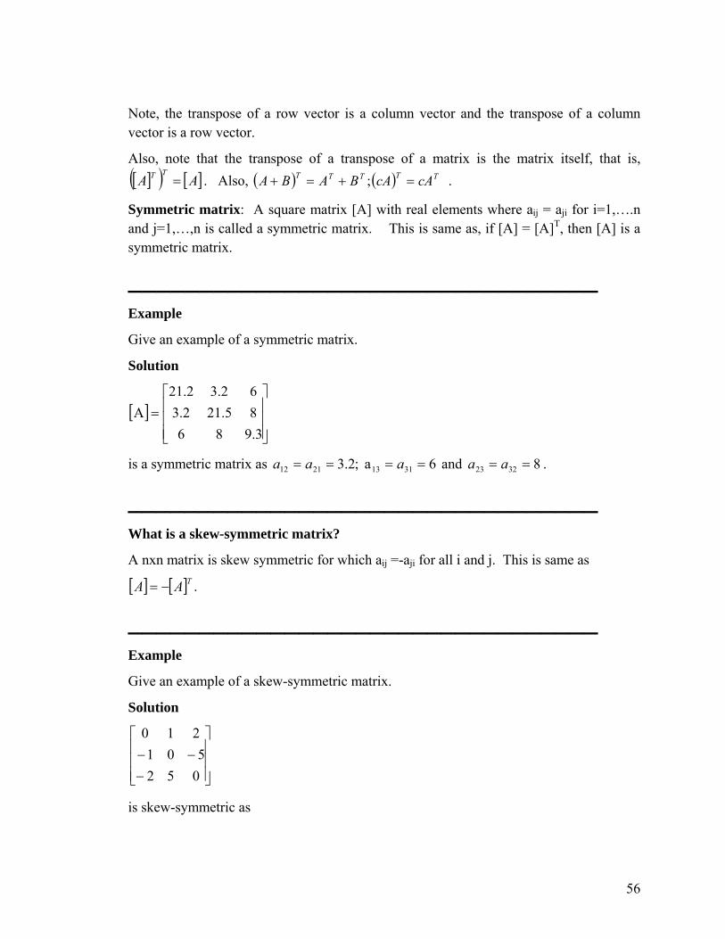
Symmetric matrix: A square matrix [A] with real elements where aij = aji for i=1,….n and j=1,…,n is called a symmetric matrix. This is same as, if [A] = [A]T, then [A] is a symmetric matrix.
_________________________________ Example
Give an example of a symmetric matrix.
Solution
[ ]⎥⎥⎥
⎦
⎤
⎢⎢⎢
⎣
⎡=
3.98685.212.362.32.21
A
is a symmetric matrix as 6a ;2.3 31132112 ==== aaa and 83223 == aa .
_________________________________ What is a skew-symmetric matrix?
A nxn matrix is skew symmetric for which aij =-aji for all i and j. This is same as
[ ] [ ] .TAA −=
_________________________________ Example
Give an example of a skew-symmetric matrix.
Solution
⎥⎥⎥
⎦
⎤
⎢⎢⎢
⎣
⎡
−−−052501
210
is skew-symmetric as
56
a12 = -a21 = 1; a13 = -a31 = 2; a23 = - a32 = -5. Since aii = -aii only if aii = 0, all the diagonal elements of a skew symmetric matrix have to be zero.
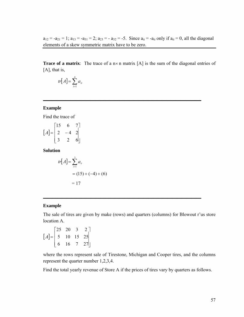
Trace of a matrix: The trace of a n×n matrix [A] is the sum of the diagonal entries of [A], that is,
[ ] ∑=
=n
iiiaAtr
1
_________________________________ Example
Find the trace of
[ ]⎥⎥⎥
⎦
⎤
⎢⎢⎢
⎣
⎡−=
6232427615
A
Solution
[ ] ∑=
=3
1iiiaAtr
)6()4()15( +−+=
= 17
_________________________________ Example
The sale of tires are given by make (rows) and quarters (columns) for Blowout r’us store location A.
[ ]⎥⎥⎥
⎦
⎤
⎢⎢⎢
⎣
⎡=
2771662515105232025
A
where the rows represent sale of Tirestone, Michigan and Cooper tires, and the columns represent the quarter number 1,2,3,4.
Find the total yearly revenue of Store A if the prices of tires vary by quarters as follows.
57

[ ]⎥⎥⎥
⎦
⎤
⎢⎢⎢
⎣
⎡=
95.2203.2702.2203.2523.3803.4102.3819.4005.3002.3501.3025.33
B
where the rows represent the cost of each tire made by Tirestone, Michigan and Cooper, the columns represent the quarter numbers.
Solution
To find the total sales of store A for the whole year, we need to find the sales of each brand of tire for the whole year and then add the total sales. To do so, we need to rewrite the price matrix so that the quarters are in rows and the brand names are in the columns, that is find transpose of [ . ]B
[ ] [ ]
T
TBC⎥⎥⎥
⎦
⎤
⎢⎢⎢
⎣
⎡==
95.2203.2702.2203.2523.3803.4102.3819.4005.3002.3501.3025.33
[ ]⎥⎥⎥⎥
⎦
⎤
⎢⎢⎢⎢
⎣
⎡
=
95.2223.3805.3003.2703.4102.3502.2202.3801.3003.2519.4025.33
C
Recognize now that if we find [A] [C], we get
[ ] [ ][ ]⎥⎥⎥⎥
⎦
⎤
⎢⎢⎢⎢
⎣
⎡
⎥⎥⎥
⎦
⎤
⎢⎢⎢
⎣
⎡==
95.2223.3805.3003.2703.4102.3502.2202.3801.3003.2519.4025.33
2771662515105232025
CAD
⎥⎥⎥
⎦
⎤
⎢⎢⎢
⎣
⎡=
131121691736132521521743119319651597
The diagonal elements give the sales of each brand of tire for the whole year, that is
d11 = $1597 (Tirestone sales)
d22 = $2152 (Michigan sales)
d33 = $1311 (Cooper sales)
58
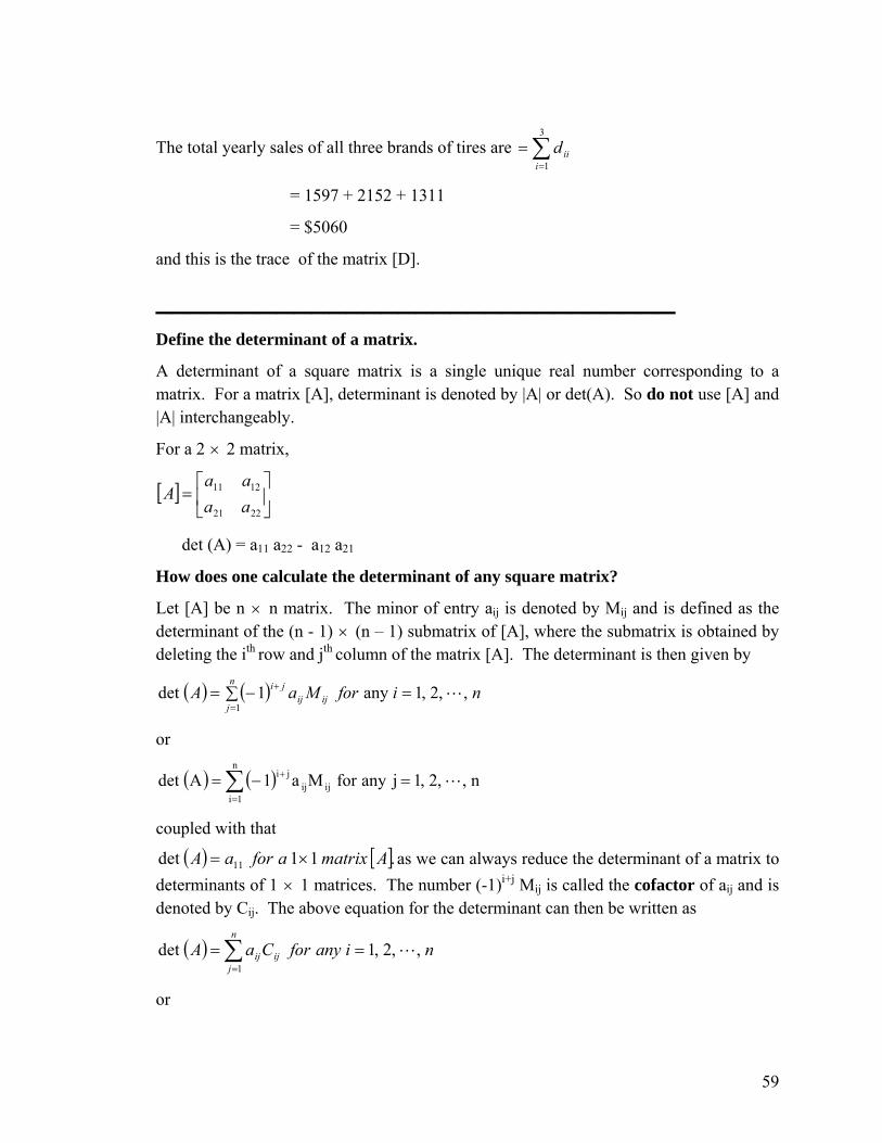
The total yearly sales of all three brands of tires are ∑=
=3
1iiid
= 1597 + 2152 + 1311
= $5060
and this is the trace of the matrix [D].
______________________________ Define the determinant of a matrix.
A determinant of a square matrix is a single unique real number corresponding to a matrix. For a matrix [A], determinant is denoted by |A| or det(A). So do not use [A] and |A| interchangeably.
For a 2 × 2 matrix,
[ ] ⎥⎦
⎤⎢⎣
⎡=
2221
1211
aaaa
A
det (A) = a11 a22 - a12 a21
How does one calculate the determinant of any square matrix?
Let [A] be n × n matrix. The minor of entry aij is denoted by Mij and is defined as the determinant of the (n - 1) × (n – 1) submatrix of [A], where the submatrix is obtained by deleting the ith row and jth column of the matrix [A]. The determinant is then given by
( ) ( )∑ =−==
+n
jijij
ji niforMaA1
,,2,1any1det L
or
( ) ( )∑=
+ =−=n
1iijij
ji n,,2,1janyforMa1Adet L
coupled with that
( ) [ ].11det 11 AmatrixaforaA ×= as we can always reduce the determinant of a matrix to determinants of 1 × 1 matrices. The number (-1)i+j Mij is called the cofactor of aij and is denoted by Cij. The above equation for the determinant can then be written as
( ) ∑=
==n
jijij nianyforCaA
1
,,2,1det L
or
59

( ) ∑=
==n
iijij njanyforCaA
1,,2,1det L
The only reason why determinants are not generally calculated using this method is that it becomes computationally intensive. For a n × n matrix, it requires arithmetic operations proportional to n!.
_________________________________ Example
Find the determinant of
[ ]⎥⎥⎥
⎦
⎤
⎢⎢⎢
⎣
⎡=
11214418641525
A
Solution
Method 1
( ) ( )∑ =−==
+3
13,2,11det
jijij
ji ianyforMaA
Let i = 1 in the formula
( ) ( )∑ −==
+3
111
11detj
jjj MaA
( ) ( ) ( ) 131331
121221
111111 111 MaMaMa +++ −+−+−=
131312121111 MaMaMa +−=
11214418641525
11 =M
11218
=
4−=
11214418641525
12 =M
60

1144164
=
80−=
11214418641525
13 =M
12144864
=
384−=
det(A) 131312121111 MaMaMa +−= ( ) ( ) ( )3841805425 −+−−−=
384400100 −+−=
84−=
Also for i=1,
( ) ∑==
3
111det
jjjCaA
( ) 1111
11 1 MC +−=
11M=
4−=
( ) 1221
12 1 MC +−=
12M−=
80=
( ) 1331
13 1 MC +−=
13M=
384−=
( ) 313121211111det CaCaCaA ++=
( ) ( ) ( 384)1(80)5(4)25( −++−= ) 384400100 −+−=
84−=
61

Method 2
( ) ( )∑ −==
+3
11det
iijij
ji MaA for any j = 1,2,3.
Let j=2 in the formula
( ) ( )∑ −==
+3
122
21deti
iii MaA
( ) ( ) ( ) 323223
222222
121221 111 MaMaMa +++ −+−+−=
323222221212 MaMaMa −+−=
11214418641525
12 =M
1144164
=
80−=
11214418641525
22 =M
1144125
=
119−=
11214418641525
32 =M
164125
= 39−=
det(A) = -5(-80) + 8(-119) – 12(-39) 323222221212 MaMaMa −+−=
= 400 – 952 + 468
= -84.
62

In terms of cofactors for j=1,
( ) ∑==
3
122det
jii CaA
( ) 1221
12 1 MC +−=
12M−=
80=
( ) 2222
22 1 MC +−=
22M=
119−=
( ) 3223
32 1 MC +−=
32M−=
39=
( ) 323222221212det CaCaCaA ++=
( ) ( ) ( )39)12(119)8(80)5( +−+=
= 400 – 952 + 468 84−=
_________________________________
Is there a relationship between det (AB), and det (A) and det (B)?
Yes, if [A] and [B] are square matrices of same size, then
det (AB) = det (A) det (B).
Are there some other theorems that are important in finding the determinant?
Theorem 1: If a row or a column in a n×n matrix [A] is zero, then det (A) =0
Theorem 2: Let [A] be a n×n matrix. If a row is proportional to another row, then det(A) = 0.
Theorem 3: Let [A] be a n×n matrix. If a column is proportional to another column, then det (A) = 0
Theorem 4: Let [A] be a n×n matrix. If a column or row is multiplied by k to result in matrix [B]. Then det(B)=k det(A).
63
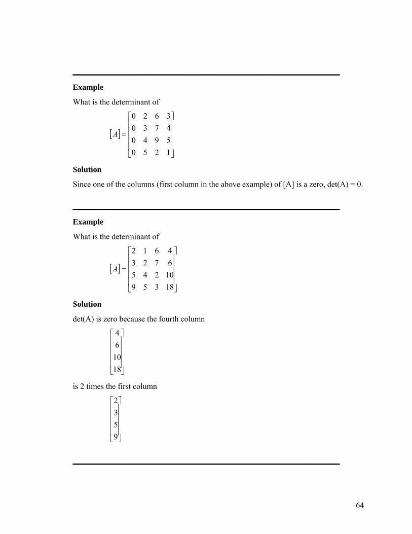
_________________________________ Example
What is the determinant of
[ ]⎥⎥⎥⎥
⎦
⎤
⎢⎢⎢⎢
⎣
⎡
=
1250594047303620
A
Solution
Since one of the columns (first column in the above example) of [A] is a zero, det(A) = 0.
_________________________________ Example
What is the determinant of
[ ]⎥⎥⎥⎥
⎦
⎤
⎢⎢⎢⎢
⎣
⎡
=
183591024567234612
A
Solution
det(A) is zero because the fourth column
⎥⎥⎥⎥
⎦
⎤
⎢⎢⎢⎢
⎣
⎡
181064
is 2 times the first column
⎥⎥⎥⎥
⎦
⎤
⎢⎢⎢⎢
⎣
⎡
9532
_________________________________
64

Example
If the determinant of
[ ]⎥⎥⎥
⎦
⎤
⎢⎢⎢
⎣
⎡=
11214418641525
A
is –84, then what is the determinant of
[ ]⎥⎥⎥
⎦
⎤
⎢⎢⎢
⎣
⎡=
12.2514418.166415.1025
B
Solution
Since the second column of [B] is 2.1 times the second column of [A],
det(B) = 2.1 det(A)
= (2.1)(-84)
= -176.4
_________________________________ Example
Given the determinant of
[ ]⎥⎥⎥
⎦
⎤
⎢⎢⎢
⎣
⎡=
11214418641525
A
is -84, what is the determinant of
[ ]⎥⎥⎥
⎦
⎤
⎢⎢⎢
⎣
⎡−−=
11214456.18.40
1525B
Solution
Since [B] is simply obtained by subtracting the second row of [A] by 2.56 times the first row of [A],
det(B) = det(A) = -84.
65

_________________________________ Example
What is the determinant of
[ ]⎥⎥⎥
⎦
⎤
⎢⎢⎢
⎣
⎡−−=
7.00056.18.40
1525A
Solution
Since [A] is an upper triangular matrix
( ) ∏=
=3
1
deti
iiaA
( )( )( )332211 aaa=
( )( )( )7.08.425 −=
= -84.
_________________________________ Key Terms
Transpose Symmetric Skew symmetric Trace Determinant
_________________________________
Homework
Let [A] = . Find [A]⎥⎦
⎤⎢⎣
⎡2976325 T 1.
Answer: ⎥⎥⎥
⎦
⎤
⎢⎢⎢
⎣
⎡
2693725
66

2.
If [A] and [B] are two symmetric matrices, show that [A]+[B] is also symmetric. nxn
Hint: Let [ ] [ ] [ ]BAC +=
ijijij bac += for all i, j.
and jijiji bac += for all i, j.
ijijji bac += as [ ]A and [ ]B are symmetric
Hence
.ijji cc =
3.
Give an example of a 4×4 symmetric matrix.
4.
Give an example of a 4×4 skew-symmetric matrix.
5.
What is the trace of
[ ]⎥⎥⎥⎥
⎦
⎤
⎢⎢⎢⎢
⎣
⎡
−
−−−−=
1032597665555
4327
A
Answer: 19
For
[ ]⎥⎥⎥
⎦
⎤
⎢⎢⎢
⎣
⎡
−−
−=
5156099.230710
A
67

Find the determinant of [A] using the cofactor method.
Answer: -150.05
6.
det (3[A]) of a n×n matrix is
a. 3 det (A)
b. det (A)
c. 3n det (A)
d. 9 det (A)
Answer (C.)
7.
For a 5×5 matrix [A], the first row is interchanged with the fifth row, the determinant of the resulting matrix [B] is
A. –det (A)
B. det (A)
C. 5 det (A)
D. 2 det (A)
Answer (A)
8.
⎥⎥⎥⎥
⎦
⎤
⎢⎢⎢⎢
⎣
⎡
0001100001000010
det is
A. 0
B. 1
C. –1
D. ∞
Answer (C.)
68
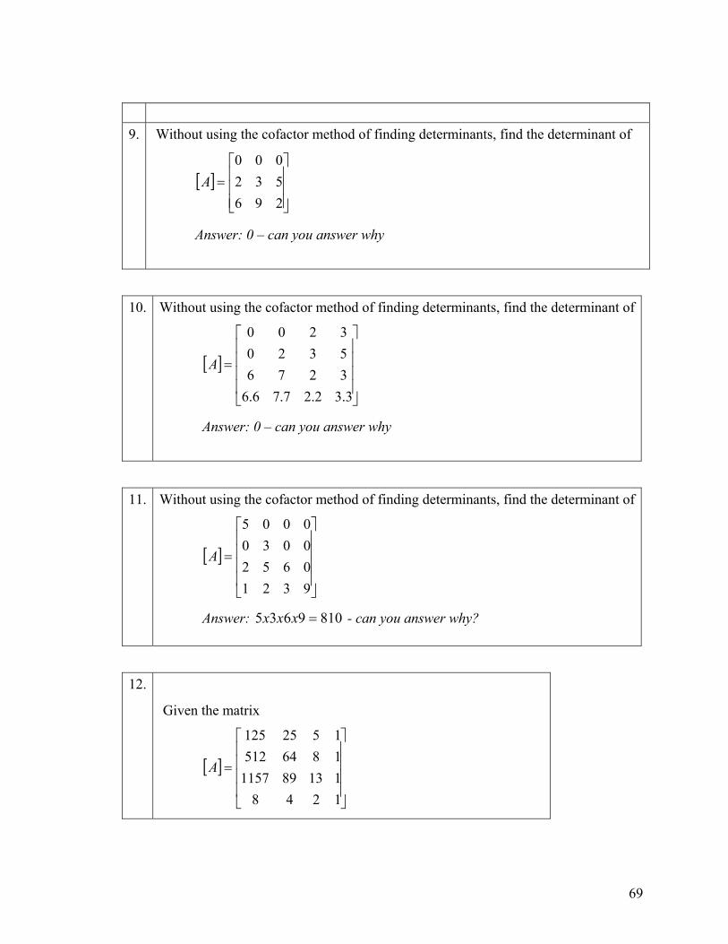
9. Without using the cofactor method of finding determinants, find the determinant of
[ ]⎥⎥⎥
⎦
⎤
⎢⎢⎢
⎣
⎡=
296532000
A
Answer: 0 – can you answer why
10. Without using the cofactor method of finding determinants, find the determinant of
[ ]⎥⎥⎥⎥
⎦
⎤
⎢⎢⎢⎢
⎣
⎡
=
3.32.27.76.6327653203200
A
Answer: 0 – can you answer why
11. Without using the cofactor method of finding determinants, find the determinant of
[ ]⎥⎥⎥⎥
⎦
⎤
⎢⎢⎢⎢
⎣
⎡
=
9321065200300005
A
Answer: 8109635 =xxx - can you answer why?
12.
Given the matrix
[ ]⎥⎥⎥⎥
⎦
⎤
⎢⎢⎢⎢
⎣
⎡
=
124811389115718645121525125
A
69

and
det(A) =-32400
find the determinant of
a) [ ]
⎥⎥⎥⎥
⎦
⎤
⎢⎢⎢⎢
⎣
⎡
−=
124819811141
18645121525125
A
b) [ ]⎥⎥⎥⎥
⎦
⎤
⎢⎢⎢⎢
⎣
⎡
=
214813189115781645125125125
A
c) [ ]
⎥⎥⎥⎥
⎦
⎤
⎢⎢⎢⎢
⎣
⎡
=
124818645121138911571525125
B
d) [ ]⎥⎥⎥⎥
⎦
⎤
⎢⎢⎢⎢
⎣
⎡
=
186451212481138911571525125
C
e) [ ]
⎥⎥⎥⎥
⎦
⎤
⎢⎢⎢⎢
⎣
⎡
=
2481611389115718645121525125
D
Answer: a) –32400 b) 32400 c) 32400 d) –32400 e) –64800
13. What is the transpose of
[A]= ⎥⎥⎥
⎦
⎤
⎢⎢⎢
⎣
⎡
2771662515105232025
70

Answer: [ ]⎥⎥⎥⎥
⎦
⎤
⎢⎢⎢⎢
⎣
⎡
=
272527153
1610206525
TA
14.
What values of the missing numbers will make this a skew-symmetric matrix?
[A]= ⎥⎥⎥
⎦
⎤
⎢⎢⎢
⎣
⎡
5?21?6??32
Answer: ⎥⎥⎥
⎦
⎤
⎢⎢⎢
⎣
⎡
−−
−
5421?4632132
15.
What values of the missing number will make this a symmetric matrix?
[A]= ⎥⎥⎥
⎦
⎤
⎢⎢⎢
⎣
⎡
5?21?6??32
Answer: ⎥⎥⎥
⎦
⎤
⎢⎢⎢
⎣
⎡
57217632132
16.
Find the determinant of
[ ] ⎥⎥⎥
⎦
⎤
⎢⎢⎢
⎣
⎡=
51214418641525
A
Answer: The determinant of [A] is
= 25(28)-5(176)+1(-384) = -564 ⎥⎦
⎤⎢⎣
⎡+⎥
⎦
⎤⎢⎣
⎡−⎥
⎦
⎤⎢⎣
⎡12144864
15144164
551218
25
71

17.
What is the determinant of an upper triangular matrix [A] that is of order nxn?
Answer: The determinant of an upper triangular matrix is the product of its diagonal elements.
18.
Given the determinant of
[ ]⎥⎥⎥
⎦
⎤
⎢⎢⎢
⎣
⎡=
aA
1214418641525
is -564, what is the determinant of [ ]⎥⎥⎥
⎦
⎤
⎢⎢⎢
⎣
⎡=
aB
1214403391525
Justify your answer?
Answer: By inspection, Row 2 of B is (Row 2-Row 1) of A. Hence, det(B) = -564. It is not necessary to find a.
19.
Why is the determinant of the following matrix zero?
[ ]⎥⎥⎥
⎦
⎤
⎢⎢⎢
⎣
⎡=
296532000
A
Answer: The first row of the matrix is zero, hence, the determinant of the matrix is zero.
20.
Why is the determinant of the following matrix zero?
[ ]⎥⎥⎥⎥
⎦
⎤
⎢⎢⎢⎢
⎣
⎡
=
3.32.27.76.6327653203200
A
Answer: Row 4 of the matrix is 1.1 times Row 3. Hence, its determinant is zero.
21.
72

Show that if [A][B]=[I], where [A], [B] and [I] are matrices of n×n size and [I] is an identity matrix, then det(A) ≠ 0 and det(B) ≠ 0.
Answer: We know that det(AB) = det(A)det(B).
[A][B] = [I]
det(AB) = det(I)
det(I) = 111 1
==∏ ∏= =
n
i
n
iiia
det(A)det(B) = 1
Therefore, det(A) ≠ 0 and det(B) ≠ 0.
73
Chapter 5 System of Equations _________________________________ After reading this chapter, you will be able to
Setup simultaneous linear equations in matrix form and vice-versa
Understand the concept of inverse of a matrix
Know the difference between consistent and inconsistent system of linear equations
Learn that system of linear equations can have a unique solution, no solution or infinite solutions
_________________________________ Matrix algebra is used for solving system of equations. Can you illustrate this concept?
Matrix algebra is used to solve a system of simultaneous linear equations. In fact, for many mathematical procedures such as solution of set of nonlinear equations, interpolation, integration, and differential equations, the solutions reduce to a set of simultaneous linear equations. Let us illustrate with an example for interpolation.
_________________________________ Example
The upward velocity of a rocket is given at three different times on the following table
Time, t Velocity, v
s m/s
5 106.8
8 177.2
12 279.2
74

The velocity data is approximated by a polynomial as
( ) 12.t5 , 2 ≤≤++= cbtattv
Set up the equations in matrix form to find the coefficients of the velocity profile. cba ,,
Solution
The polynomial is going through three data points ( ) ( ) ( 332211 ,t and ,, ,, vvtvt ) where from the above table
8.106,5 11 == vt
2.177,8 22 == vt
2.279,12 33 == vt
Requiring that passes through the three data points gives ( ) cbtattv ++= 2
( ) cbtatvtv ++== 12111
( ) cbtatvtv ++== 22222
( ) cbtatvtv ++== 32333
Substituting the data ( ) ( ) ( )332211 , , , , , vtvtvt gives
( ) ( ) 8.106552 =++ cba
( ) ( ) 2.177882 =++ cba
( ) ( ) 2.27912122 =++ cba
or
8.106525 =++ cba
2.177864 =++ cba
2.27912144 =++ cba
This set of equations can be rewritten in the matrix form as
⎥⎥⎥
⎦
⎤
⎢⎢⎢
⎣
⎡=
⎥⎥⎥
⎦
⎤
⎢⎢⎢
⎣
⎡
++++++
2.2792.1778.106
12144864525
cbacbacba
The above equation can be written as a linear combination as follows
75

⎥⎥⎥
⎦
⎤
⎢⎢⎢
⎣
⎡=
⎥⎥⎥
⎦
⎤
⎢⎢⎢
⎣
⎡+
⎥⎥⎥
⎦
⎤
⎢⎢⎢
⎣
⎡+
⎥⎥⎥
⎦
⎤
⎢⎢⎢
⎣
⎡
2.2792.1778.106
111
1285
1446425
cba
and further using matrix multiplications gives
⎥⎥⎥
⎦
⎤
⎢⎢⎢
⎣
⎡=
⎥⎥⎥
⎦
⎤
⎢⎢⎢
⎣
⎡
⎥⎥⎥
⎦
⎤
⎢⎢⎢
⎣
⎡
2.2792.1778.106
cba
11214418641525
_________________________________ The above is an illustration of why matrix algebra is needed. The complete solution to the set of equations is given later in this chapter.
For a general set of “m” linear equations and “n” unknowns,
11222111 cxaxaxa nn =+++ LL
22222121 cxaxaxa nn =+++ LL
……………………………………
…………………………………….
mnmnmm cxaxaxa =+++ ........2211
can be rewritten in the matrix form as
⎥⎥⎥⎥⎥⎥
⎦
⎤
⎢⎢⎢⎢⎢⎢
⎣
⎡
⋅⋅=
⎥⎥⎥⎥⎥⎥
⎦
⎤
⎢⎢⎢⎢⎢⎢
⎣
⎡
⋅⋅
⎥⎥⎥⎥⎥⎥
⎦
⎤
⎢⎢⎢⎢⎢⎢
⎣
⎡
mnmnmm
n
n
c
cc
x
xx
aaa
aaaaaa
2
1
2
1
21
22221
11211
..
..
..
MM
MM
Denoting the matrices by , [ ]A [ ]X , and [ ]C , the system of equation is
[ ]A = [ , where [ is called the coefficient matrix, [ ]X ]C ]A [ ]C is called the right hand side vector and [ is called the solution vector. ]X
Sometimes = systems of equations is written in the augmented form. That is
[ ]A [ ]X [ ]C
76
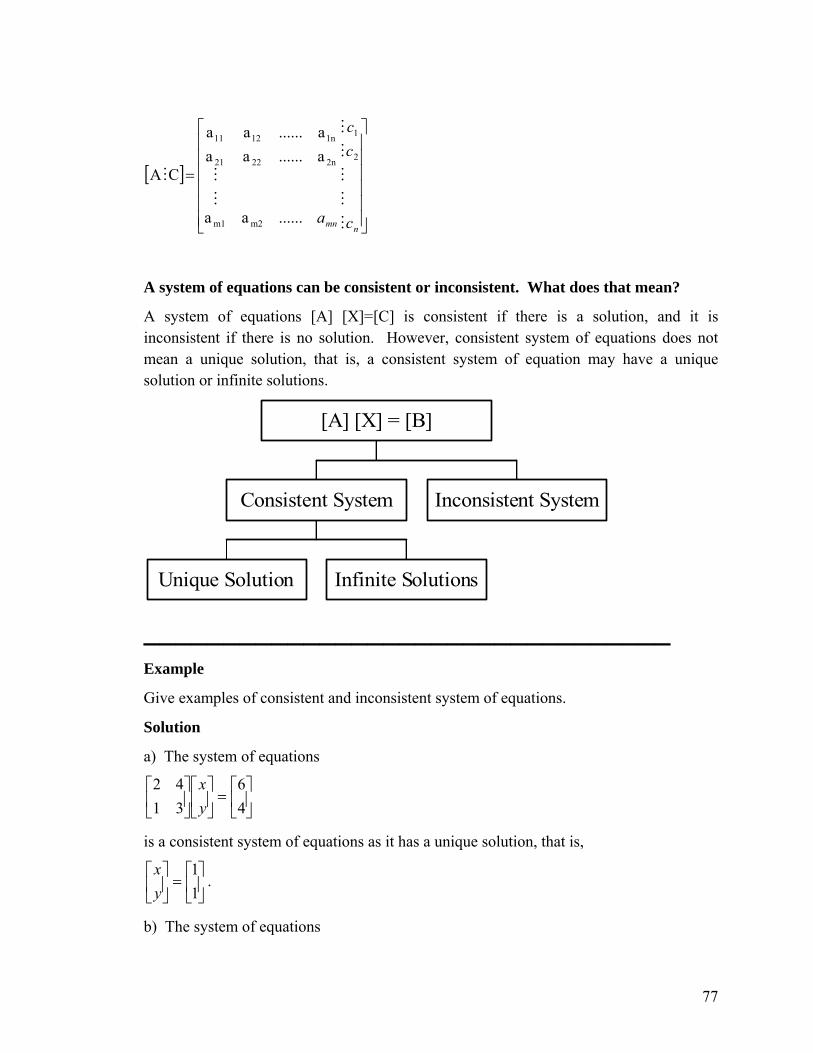
[ ]
⎥⎥⎥⎥⎥⎥
⎦
⎤
⎢⎢⎢⎢⎢⎢
⎣
⎡
=
nmn c
cc
a
2
1
m2m1
2n2221
1n1211
......aa
a......aaa......aa
CA
M
M
M
M
M
M
MM
A system of equations can be consistent or inconsistent. What does that mean?
A system of equations [A] [X]=[C] is consistent if there is a solution, and it is inconsistent if there is no solution. However, consistent system of equations does not mean a unique solution, that is, a consistent system of equation may have a unique solution or infinite solutions.
Unique Solution Infinite Solutions
Consistent System Inconsistent System
[A] [X] = [B]
_________________________________ Example
Give examples of consistent and inconsistent system of equations.
Solution
a) The system of equations
⎥⎦
⎤⎢⎣
⎡=⎥
⎦
⎤⎢⎣
⎡⎥⎦
⎤⎢⎣
⎡46
3142
yx
is a consistent system of equations as it has a unique solution, that is,
⎥⎦
⎤⎢⎣
⎡=⎥
⎦
⎤⎢⎣
⎡11
yx
.
b) The system of equations
77
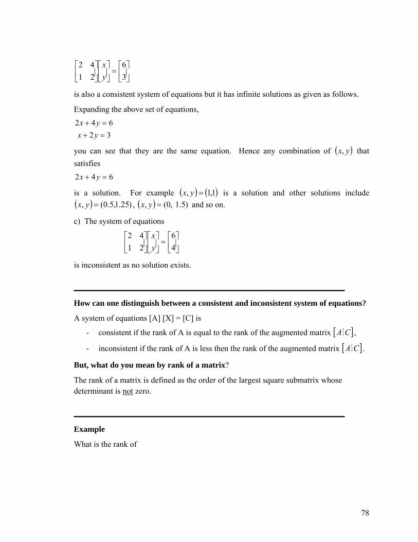
⎥⎦
⎤⎢⎣
⎡=⎥
⎦
⎤⎢⎣
⎡⎥⎦
⎤⎢⎣
⎡36
2142
yx
is also a consistent system of equations but it has infinite solutions as given as follows.
Expanding the above set of equations,
32642
=+=+
yxyx
you can see that they are the same equation. Hence any combination of that satisfies
( yx, )
642 =+ yx
is a solution. For example ( ) ( )1,1, =yx is a solution and other solutions include , ( ) and so on. ( ) )25.1,5.0(, =yx )5.1 ,0(, =yx
c) The system of equations
⎥⎦
⎤⎢⎣
⎡=⎥
⎦
⎤⎢⎣
⎡⎥⎦
⎤⎢⎣
⎡46
2142
yx
is inconsistent as no solution exists.
_________________________________ How can one distinguish between a consistent and inconsistent system of equations?
A system of equations [A] [X] = [C] is
- consistent if the rank of A is equal to the rank of the augmented matrix , [ ]CAM
- inconsistent if the rank of A is less then the rank of the augmented matrix [ ]CAM .
But, what do you mean by rank of a matrix?
The rank of a matrix is defined as the order of the largest square submatrix whose determinant is not zero.
_________________________________ Example
What is the rank of
78

[ ]⎥⎥⎥
⎦
⎤
⎢⎢⎢
⎣
⎡=
321502213
A
Solution
The largest square submatrix possible is of order 3 and that is [A] itself. Since det(A) = -25 ≠ 0, the rank of [A] = 3.
_________________________________ Example
What is the rank of
[ ]⎥⎥⎥
⎦
⎤
⎢⎢⎢
⎣
⎡=
715502213
A
Solution
The largest square submatrix of [A] is of order 3, and is [A] itself. Since det(A) = 0, the rank of [A] is less than 3. The next largest square submatrix would be a 2 2 matrix. One of the square submatrices of [A] is
×
[ ] ⎥⎦
⎤⎢⎣
⎡=
0213
B
and det [B] = -2 ≠ 0. Hence the rank of [A] is 2.
_________________________________ Example
How do I now use the concept of rank to find if
⎥⎥⎥
⎦
⎤
⎢⎢⎢
⎣
⎡=
⎥⎥⎥
⎦
⎤
⎢⎢⎢
⎣
⎡
⎥⎥⎥
⎦
⎤
⎢⎢⎢
⎣
⎡
2.2792.1778.106
11214418641525
3
2
1
xxx
is a consistent or inconsistent system of equations?
Solution
The coefficient matrix is
79

[ ]⎥⎥⎥
⎦
⎤
⎢⎢⎢
⎣
⎡=
11214418641525
A
and the right hand side vector
. [ ]⎥⎥⎥
⎦
⎤
⎢⎢⎢
⎣
⎡=
2.2792.1778.106
C
The augmented matrix is
[ ]⎥⎥⎥
⎦
⎤
⎢⎢⎢
⎣
⎡=
2.2791121442.17718648.1061525
M
M
M
B
Since there are no square submatrices of order 4 as [B] is a 3x4 matrix, the rank of [B] is at most 3. So let us look at the square submatrices of [B] of order 3 and if any of these square submatrices have determinant not equal to zero, then the rank is 3. For example, a submatrix of the augmented matrix [B] is
⎥⎥⎥
⎦
⎤
⎢⎢⎢
⎣
⎡=
11214418641525
][D
has det (D) = -84 ≠ 0.
Hence the rank of the augmented matrix [B] is 3. Since [A]=[D] , the rank of [A] =3. Since the rank of augmented matrix [B] = rank of coefficient matrix [A], the system of equations is consistent.
_________________________________ Example
Use the concept of rank of matrix to find if
⎥⎥⎥
⎦
⎤
⎢⎢⎢
⎣
⎡=
⎥⎥⎥
⎦
⎤
⎢⎢⎢
⎣
⎡
⎥⎥⎥
⎦
⎤
⎢⎢⎢
⎣
⎡
0.2842.1778.106
2138918641525
3
2
1
xxx
is consistent or inconsistent?
Solution
80

The coefficient matrix is given by
[ ]⎥⎥⎥
⎦
⎤
⎢⎢⎢
⎣
⎡=
2138918641525
A
and the right hand side
[ ]⎥⎥⎥
⎦
⎤
⎢⎢⎢
⎣
⎡=
0.2842.1778.106
C
The augmented matrix is
[ ]⎥⎥⎥
⎦
⎤
⎢⎢⎢
⎣
⎡=
0.284213892.17718648.1061525
B
Since there are no square submatrices of order 4 as [B] is a 4×3 matrix, the rank of the augmented [B] is at most 3. So let us look at square submatrices of the augmented matrix [B] of order 3 and see if any of these square submatrices have determinant not equal to zero, then the rank is 3. For example a square submatrix of the augmented matrix [B] is
[ ]⎥⎥⎥
⎦
⎤
⎢⎢⎢
⎣
⎡=
2138918641525
D
has det(D) = 0. This means, we need to explore other square submatrices of order 3 of the augmented matrix [B].
That is,
[ ]⎥⎥⎥
⎦
⎤
⎢⎢⎢
⎣
⎡=
0.2842132.177188.10615
E
det(E) = 0,
[ ]⎥⎥⎥
⎦
⎤
⎢⎢⎢
⎣
⎡=
0.28413892.1778648.106525
F
det(F) = 0,
81
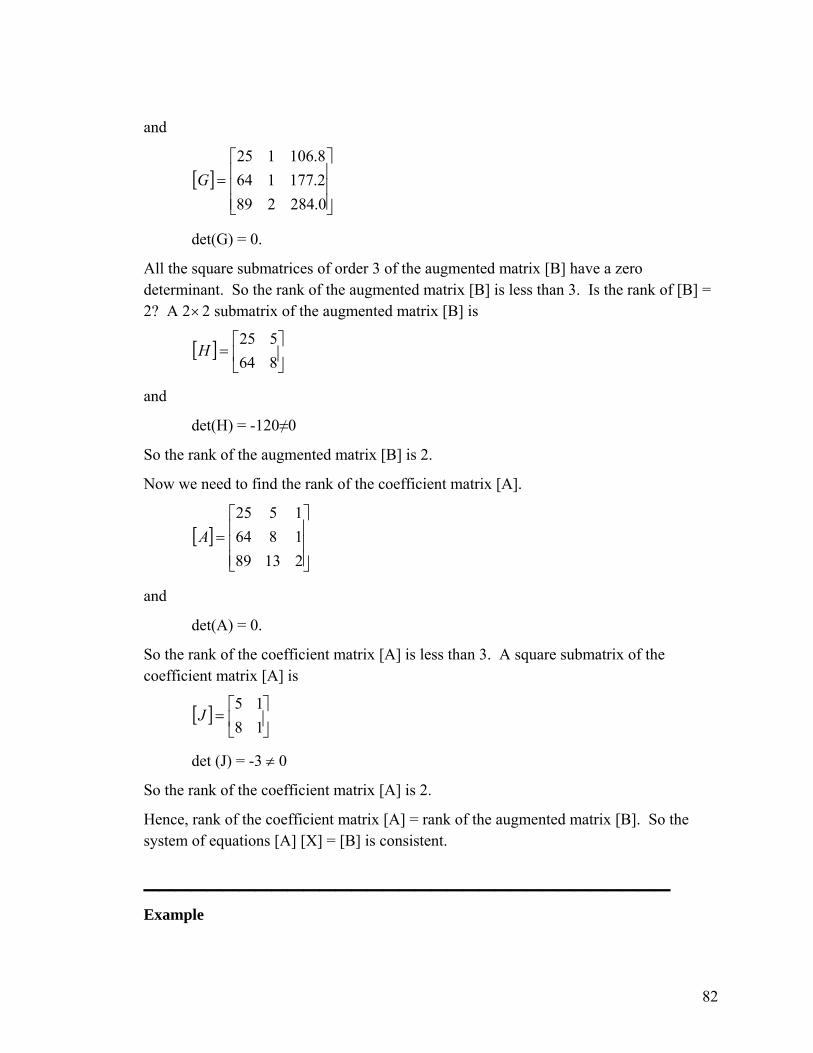
and
[ ]⎥⎥⎥
⎦
⎤
⎢⎢⎢
⎣
⎡=
0.2842892.1771648.106125
G
det(G) = 0.
All the square submatrices of order 3 of the augmented matrix [B] have a zero determinant. So the rank of the augmented matrix [B] is less than 3. Is the rank of [B] = 2? A 2×2 submatrix of the augmented matrix [B] is
[ ] ⎥⎦
⎤⎢⎣
⎡=
864525
H
and
det(H) = -120≠0
So the rank of the augmented matrix [B] is 2.
Now we need to find the rank of the coefficient matrix [A].
[ ]⎥⎥⎥
⎦
⎤
⎢⎢⎢
⎣
⎡=
2138918641525
A
and
det(A) = 0.
So the rank of the coefficient matrix [A] is less than 3. A square submatrix of the coefficient matrix [A] is
[ ] ⎥⎦
⎤⎢⎣
⎡=
1815
J
det (J) = -3 ≠ 0
So the rank of the coefficient matrix [A] is 2.
Hence, rank of the coefficient matrix [A] = rank of the augmented matrix [B]. So the system of equations [A] [X] = [B] is consistent.
_________________________________ Example
82

Use the concept of rank to find if
⎥⎥⎥
⎦
⎤
⎢⎢⎢
⎣
⎡=
⎥⎥⎥
⎦
⎤
⎢⎢⎢
⎣
⎡
⎥⎥⎥
⎦
⎤
⎢⎢⎢
⎣
⎡
0.2802.1778.106
xxx
2138918641525
3
2
1
is consistent or inconsistent.
Solution
The augmented matrix is
[ ]⎥⎥⎥
⎦
⎤
⎢⎢⎢
⎣
⎡=
0.280213892.17748648.1061525
B
Since there are no square submatrices of order 4 as the augmented matrix [B] is a 4×3 matrix, the rank of the augmented matrix [B] is at most 3. So let us look at square submatrices of the augmented matrix (B) of order 3 and see if any of the 3×3 submatrices have a determinant not equal to zero. For example a square submatrix of order 3×3 of [B]
[ ]⎥⎥⎥
⎦
⎤
⎢⎢⎢
⎣
⎡=
2138918641525
D
det(D) = 0
So it means, we need to explore other square submatrices of the augmented matrix [B],
[ ]⎥⎥⎥
⎦
⎤
⎢⎢⎢
⎣
⎡=
0.2802132.177188.10615
E
det(E) ≠ 12.0 ≠ 0.
So rank of the augmented matrix [B] = 3.
The rank of the coefficient matrix [A] = 2 from the previous example.
Since rank of the coefficient matrix [A] < rank of the augmented matrix [B], the system of equations is inconsistent. Hence no solution exists for [A] [X] = [C].
_________________________________
83
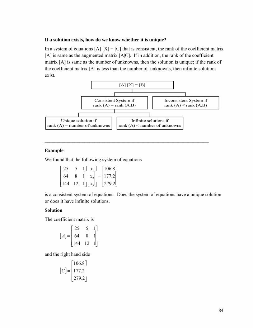
If a solution exists, how do we know whether it is unique?
In a system of equations [A] [X] = [C] that is consistent, the rank of the coefficient matrix [A] is same as the augmented matrix [A|C]. If in addition, the rank of the coefficient matrix [A] is same as the number of unknowns, then the solution is unique; if the rank of the coefficient matrix [A] is less than the number of unknowns, then infinite solutions exist.
Unique solution ifrank (A) = number of unknowns
Infinite solutions ifrank (A) < number of unknowns
Consistent System ifrank (A) = rank (A.B)
Inconsistent System ifrank (A) < rank (A.B)
[A] [X] = [B]
_________________________________ Example:
We found that the following system of equations
⎥⎥⎥
⎦
⎤
⎢⎢⎢
⎣
⎡=
⎥⎥⎥
⎦
⎤
⎢⎢⎢
⎣
⎡
⎥⎥⎥
⎦
⎤
⎢⎢⎢
⎣
⎡
2.2792.1778.106
11214418641525
3
2
1
xxx
is a consistent system of equations. Does the system of equations have a unique solution or does it have infinite solutions.
Solution
The coefficient matrix is
[ ]⎥⎥⎥
⎦
⎤
⎢⎢⎢
⎣
⎡=
11214418641525
A
and the right hand side
[ ]⎥⎥⎥
⎦
⎤
⎢⎢⎢
⎣
⎡=
2.2792.1778.106
C
84
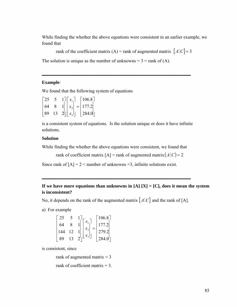
While finding the whether the above equations were consistent in an earlier example, we found that
rank of the coefficient matrix (A) = rank of augmented matrix [ ] 3=CAM
The solution is unique as the number of unknowns = 3 = rank of (A).
________________________________ Example:
We found that the following system of equations
⎥⎥⎥
⎦
⎤
⎢⎢⎢
⎣
⎡=
⎥⎥⎥
⎦
⎤
⎢⎢⎢
⎣
⎡
⎥⎥⎥
⎦
⎤
⎢⎢⎢
⎣
⎡
0.2842.1778.106
2138918641525
3
2
1
xxx
is a consistent system of equations. Is the solution unique or does it have infinite solutions.
Solution
While finding the whether the above equations were consistent, we found that
rank of coefficient matrix [A] = rank of augmented matrix ( ) 2=CAM
Since rank of [A] = 2 < number of unknowns =3, infinite solutions exist.
________________________________ If we have more equations than unknowns in [A] [X] = [C], does it mean the system is inconsistent?
No, it depends on the rank of the augmented matrix [ ]CAM and the rank of [A].
a) For example
⎥⎥⎥⎥
⎦
⎤
⎢⎢⎢⎢
⎣
⎡
=⎥⎥⎥
⎦
⎤
⎢⎢⎢
⎣
⎡
⎥⎥⎥⎥
⎦
⎤
⎢⎢⎢⎢
⎣
⎡
0.2842.2792.1778.106
2138911214418641525
3
2
1
xxx
is consistent, since
rank of augmented matrix = 3
rank of coefficient matrix = 3.
85

Now since rank of (A) = 3 = number of unknowns, the solution is not only consistent but also unique.
b) For example
⎥⎥⎥⎥
⎦
⎤
⎢⎢⎢⎢
⎣
⎡
=⎥⎥⎥
⎦
⎤
⎢⎢⎢
⎣
⎡
⎥⎥⎥⎥
⎦
⎤
⎢⎢⎢⎢
⎣
⎡
0.2802.2792.1778.106
2138911214418641525
3
2
1
xxx
is inconsistent, since
rank of augmented matrix = 4
rank of coefficient matrix = 3.
c) For example
⎥⎥⎥⎥
⎦
⎤
⎢⎢⎢⎢
⎣
⎡
=⎥⎥⎥
⎦
⎤
⎢⎢⎢
⎣
⎡
⎥⎥⎥⎥
⎦
⎤
⎢⎢⎢⎢
⎣
⎡
0.2806.2132.1778.106
213892105018641525
3
2
1
xxx
is consistent, since
rank of augmented matrix = 2
rank of coefficient matrix = 2.
But since the rank of [A] = 2 < the number of unknowns = 3, infinite solutions exist.
Consistent system of equations can only have a unique solution or infinite solutions. Can a system of equations have a finite (more than one but not infinite) number of solutions?
No, you can only have a unique solution or infinite solutions. Let us suppose [A] [X]=[C] has two solutions [Y] and [Z] so that
[A] [Y]=[C]
[A] [Z]=[C]
If r is a constant, then from the two equations
[ ][ ] [ ]CrAr =Y
( )[ ][ ] ( )[ ]CrAr −=− 1Z 1
86
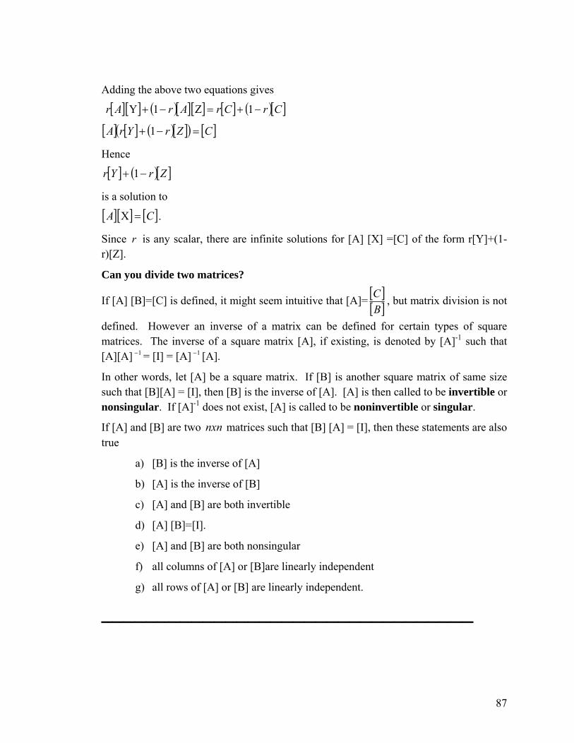
Adding the above two equations gives
[ ][ ] ( )[ ][ ] [ ] ( )[ ]CrCrArAr −+=−+ 1Z 1Y
[ ] [ ] ( )[ ]( ) [ ]CZrYrA =−+ 1
Hence
[ ] ( )[ ]ZrYr −+ 1
is a solution to
[ ][ ] [ ]CA =X .
Since r is any scalar, there are infinite solutions for [A] [X] =[C] of the form r[Y]+(1-r)[Z].
Can you divide two matrices?
If [A] [B]=[C] is defined, it might seem intuitive that [A]= [ ][ ]BC , but matrix division is not
defined. However an inverse of a matrix can be defined for certain types of square matrices. The inverse of a square matrix [A], if existing, is denoted by [A]-1 such that [A][A] = [I] = [A] [A]. 1− 1−
In other words, let [A] be a square matrix. If [B] is another square matrix of same size such that [B][A] = [I], then [B] is the inverse of [A]. [A] is then called to be invertible or nonsingular. If [A]-1 does not exist, [A] is called to be noninvertible or singular.
If [A] and [B] are two nxn matrices such that [B] [A] = [I], then these statements are also true
a) [B] is the inverse of [A]
b) [A] is the inverse of [B]
c) [A] and [B] are both invertible
d) [A] [B]=[I].
e) [A] and [B] are both nonsingular
f) all columns of [A] or [B]are linearly independent
g) all rows of [A] or [B] are linearly independent.
_________________________________
87
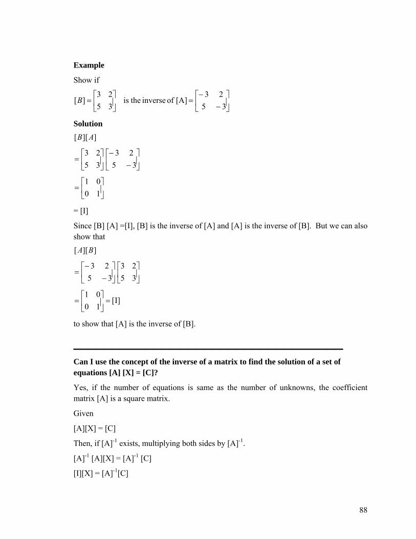
Example
Show if
⎥⎦
⎤⎢⎣
⎡−
−=⎥
⎦
⎤⎢⎣
⎡=
3523
[A] of inverse theis3523
][B
Solution ]][[ AB
⎥⎦
⎤⎢⎣
⎡−
−⎥⎦
⎤⎢⎣
⎡=
3523
3523
1001⎥⎦
⎤⎢⎣
⎡=
= [I]
Since [B] [A] =[I], [B] is the inverse of [A] and [A] is the inverse of [B]. But we can also show that
]][[ BA
⎥⎦
⎤⎢⎣
⎡⎥⎦
⎤⎢⎣
⎡−
−=
3523
3523
I][1001
=⎥⎦
⎤⎢⎣
⎡=
to show that [A] is the inverse of [B].
_________________________________ Can I use the concept of the inverse of a matrix to find the solution of a set of equations [A] [X] = [C]?
Yes, if the number of equations is same as the number of unknowns, the coefficient matrix [A] is a square matrix.
Given
[A][X] = [C]
Then, if [A]-1 exists, multiplying both sides by [A]-1.
[A]-1 [A][X] = [A]-1 [C]
[I][X] = [A]-1[C]
88
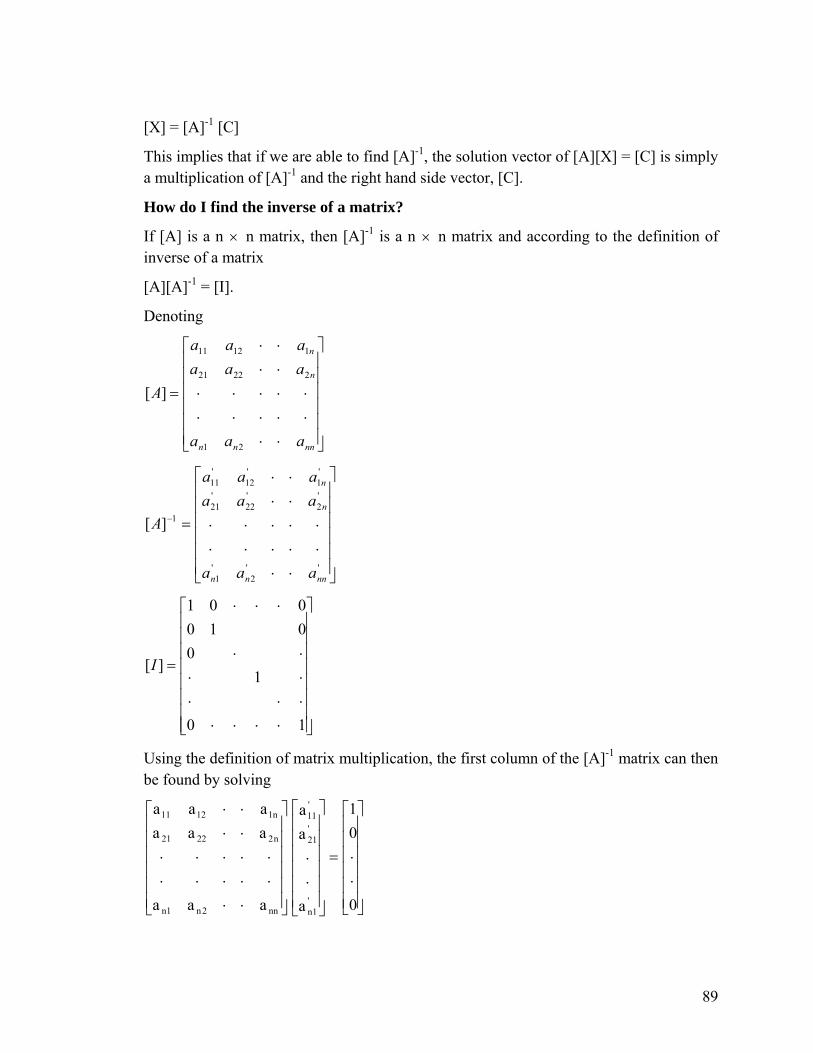
[X] = [A]-1 [C]
This implies that if we are able to find [A]-1, the solution vector of [A][X] = [C] is simply a multiplication of [A]-1 and the right hand side vector, [C].
How do I find the inverse of a matrix?
If [A] is a n × n matrix, then [A]-1 is a n × n matrix and according to the definition of inverse of a matrix
[A][A]-1 = [I].
Denoting
⎥⎥⎥⎥⎥⎥
⎦
⎤
⎢⎢⎢⎢⎢⎢
⎣
⎡
⋅⋅⋅⋅⋅⋅⋅⋅⋅⋅⋅⋅
⋅⋅⋅⋅
=
nnnn
n
n
aaa
aaaaaa
A
21
22221
11211
][
⎥⎥⎥⎥⎥⎥
⎦
⎤
⎢⎢⎢⎢⎢⎢
⎣
⎡
⋅⋅⋅⋅⋅⋅⋅⋅⋅⋅⋅⋅
⋅⋅⋅⋅
=−
''2
'1
'2
'22
'21
'1
'12
'11
1][
nnnn
n
n
aaa
aaaaaa
A
⎥⎥⎥⎥⎥⎥⎥⎥
⎦
⎤
⎢⎢⎢⎢⎢⎢⎢⎢
⎣
⎡
⋅⋅⋅⋅⋅⋅⋅⋅⋅⋅⋅
⋅⋅⋅
=
10
10
010001
][I
Using the definition of matrix multiplication, the first column of the [A]-1 matrix can then be found by solving
⎥⎥⎥⎥⎥⎥
⎦
⎤
⎢⎢⎢⎢⎢⎢
⎣
⎡
⋅⋅=
⎥⎥⎥⎥⎥⎥
⎦
⎤
⎢⎢⎢⎢⎢⎢
⎣
⎡
⋅⋅
⎥⎥⎥⎥⎥⎥
⎦
⎤
⎢⎢⎢⎢⎢⎢
⎣
⎡
⋅⋅⋅⋅⋅⋅⋅⋅⋅⋅⋅⋅
⋅⋅⋅⋅
0
01
a
aa
aaa
aaaaaa
'1n
'21
'11
nn2n1n
n22221
n11211
89

Similarly, one can find the other columns of the [A]-1 matrix by changing the right hand side accordingly.
_________________________________
Example
The upward velocity of the rocket is given by
Time, t Velocity
s m/s
5 106.8
8 177.2
12 279.2
In an earlier example, we wanted to approximate the velocity profile by ( ) 1285 ,2 ≤≤++= cbtattv
We found that the coefficients are given by cba ,,
⎥⎥⎥
⎦
⎤
⎢⎢⎢
⎣
⎡=
⎥⎥⎥
⎦
⎤
⎢⎢⎢
⎣
⎡
⎥⎥⎥
⎦
⎤
⎢⎢⎢
⎣
⎡
2.2792.1778.106
cba
11214418641525
First find the inverse of
[ ]⎥⎥⎥
⎦
⎤
⎢⎢⎢
⎣
⎡=
11214418641525
A
and then use the definition of inverse to find the coefficients .,, cba
Solution
If [ ]⎥⎥⎥
⎦
⎤
⎢⎢⎢
⎣
⎡
=−
'33
'32
'31
'23
'22
'21
'13
'12
'11
1
aaaaaaaaa
A
is the inverse of [A],
90

Then
⎥⎥⎥
⎦
⎤
⎢⎢⎢
⎣
⎡=
⎥⎥⎥
⎦
⎤
⎢⎢⎢
⎣
⎡
⎥⎥⎥
⎦
⎤
⎢⎢⎢
⎣
⎡
100010001
11214418641525
'33
'32
'31
'23
'22
'21
'13
'12
'11
aaaaaaaaa
gives three sets of equations
⎥⎥⎥
⎦
⎤
⎢⎢⎢
⎣
⎡=
⎥⎥⎥
⎦
⎤
⎢⎢⎢
⎣
⎡
⎥⎥⎥
⎦
⎤
⎢⎢⎢
⎣
⎡
001
11214418641525
'31
'21
'11
aaa
⎥⎥⎥
⎦
⎤
⎢⎢⎢
⎣
⎡=
⎥⎥⎥
⎦
⎤
⎢⎢⎢
⎣
⎡
⎥⎥⎥
⎦
⎤
⎢⎢⎢
⎣
⎡
010
11214418641525
'32
'22
'12
aaa
⎥⎥⎥
⎦
⎤
⎢⎢⎢
⎣
⎡=
⎥⎥⎥
⎦
⎤
⎢⎢⎢
⎣
⎡
⎥⎥⎥
⎦
⎤
⎢⎢⎢
⎣
⎡
100
11214418641525
'33
'23
'13
aaa
Solving the above three sets of equations separately gives
⎥⎥⎥
⎦
⎤
⎢⎢⎢
⎣
⎡
'31
'21
'11
aaa
= ⎥⎥⎥
⎦
⎤
⎢⎢⎢
⎣
⎡−
571.49524.0
04762.0
⎥⎥⎥
⎦
⎤
⎢⎢⎢
⎣
⎡
'32
'22
'12
aaa
= ⎥⎥⎥
⎦
⎤
⎢⎢⎢
⎣
⎡
−
−
000.5417.108333.0
⎥⎥⎥
⎦
⎤
⎢⎢⎢
⎣
⎡−=
⎥⎥⎥
⎦
⎤
⎢⎢⎢
⎣
⎡
429.14643.0
03571.0
'33
'23
'13
aaa
Hence
⎥⎥⎥
⎦
⎤
⎢⎢⎢
⎣
⎡
−−−
−=−
429.1000.5571.44643.0417.19524.0
03571.008333.004762.0][ 1A
Now
91

[ ][ ] [ ]CA =X
where
[ ]⎥⎥⎥
⎦
⎤
⎢⎢⎢
⎣
⎡=
cba
X
[ ]⎥⎥⎥
⎦
⎤
⎢⎢⎢
⎣
⎡=
2.2792.1778.106
C
Using the definition of [ ] ,1−A
[ ] [ ][ ] [ ] [ ] C X A 11 −− = AA
[ ] [ ] [ ]C X 1−= A
279.2177.2106.8
1.4295.000-4.5710.4643-1.4170.9524-
0.035710.08333-0.04762-
⎥⎥⎥
⎦
⎤
⎢⎢⎢
⎣
⎡
⎥⎥⎥
⎦
⎤
⎢⎢⎢
⎣
⎡=
⎥⎥⎥
⎦
⎤
⎢⎢⎢
⎣
⎡=
⎥⎥⎥
⎦
⎤
⎢⎢⎢
⎣
⎡
050.170.19
2900.0
cba
So
( ) 12t5 ,050.170.192900.0 2 ≤≤++= tttv
Is there another way to find the inverse of a matrix?
For finding inverse of small matrices, inverse of an invertible matrix can be found by
[ ] ( ) ( )AadjA
Adet
11 =−
where
( )
T
nnnn
n
n
CCC
CCCCCC
Aadj
⎥⎥⎥⎥
⎦
⎤
⎢⎢⎢⎢
⎣
⎡
−
=
21
22221
11211
M
L
92

where Cij are the cofactors of aij. The matrix itself is called the
matrix of cofactors from [A]. Cofactors are defined in Chapter 4.
⎥⎥⎥⎥
⎦
⎤
⎢⎢⎢⎢
⎣
⎡
nnn
n
n
CC
CCCCCC
LL
MM
L
L
1
22222
11211
Example
Find the inverse of
[ ]⎥⎥⎥
⎦
⎤
⎢⎢⎢
⎣
⎡=
11214418641525
A
Solution
From the example in Chapter 4, we found
. ( ) 84det −=A
Next we need to find the adjoint of [A]. The cofactors of A are found as follows.
The minor of entry a11 is
11214418641525
11 =M
11218
=
4−=
The cofactors of entry a11 is
( ) 41 111111
11 −==−= + MMC
The minor of entry a12 is
11214418641525
12 =M
1144164
=
93

80−=
The cofactor of entry a12 is
( ) 1221
12 1 MC +−=
12M−=
80=
Similarly
38413 =C
721 =C
11922 −=C
42023 =C
331 −=C
3932 =C
12033 −=C
Hence the matrix of cofactors of [A] is
[ ]⎥⎥⎥
⎦
⎤
⎢⎢⎢
⎣
⎡
−−−
−−=
1203934201197384804
C
The adjoint of matrix [A] is [C]T,
( ) [ ]⎥⎥⎥
⎦
⎤
⎢⎢⎢
⎣
⎡
−−−
−−==
1204203843911980
374TCAadj
Hence
[ ] ( ) ( )AadjA
Adet
11 =−
⎥⎥⎥
⎦
⎤
⎢⎢⎢
⎣
⎡
−−−
−−
−=
1204203843911980
374
841
94

⎥⎥⎥
⎦
⎤
⎢⎢⎢
⎣
⎡
−−−
−=
429.1000.5571.44643.0417.19524.0
03571.008333.004762.0
_________________________________ If the inverse of a square matrix [A] exists, is it unique?
Yes, the inverse of a square matrix is unique, if it exists. The proof is as follows. Assume that the inverse of [A] is [B] and if this inverse is not unique, then let another inverse of [A] exist called [C].
[B] is inverse of [A], then
[B][A] = [I]
Multiply both sides by [C],
[B][A][C] = [I][C]
[B][A][C] = [C]
Since [C] is inverse of [A], [A][C] = [I]
[B][I] = [C]
[B] = [C]
This shows that [B] and [C] are the same. So inverse of [A] is unique.
_________________________________ Key Terms
Consistent system Inconsistent system
Infinite solutions Unique solution
Rank Inverse
_________________________________ Homework
1. For a set of equations [A] [X] = [B], a unique solution exists if
95
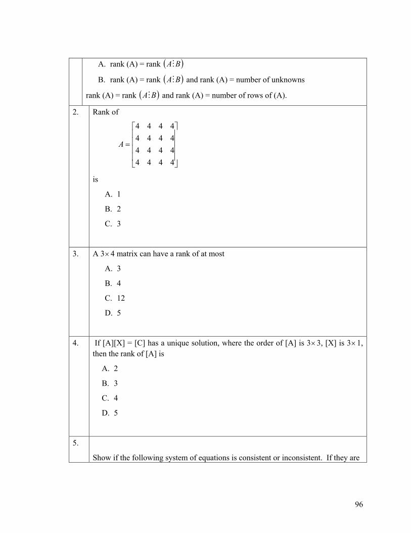
A. rank (A) = rank ( )BAM
B. rank (A) = rank and rank (A) = number of unknowns ( BAM ))rank (A) = rank and rank (A) = number of rows of (A). ( BAM
2. Rank of
⎥⎥⎥⎥
⎦
⎤
⎢⎢⎢⎢
⎣
⎡
=
4444444444444444
A
is
A. 1
B. 2
C. 3
3. A 3×4 matrix can have a rank of at most
A. 3
B. 4
C. 12
D. 5
If [A][X] = [C] has a unique solution, where the order of [A] is 3×3, [X] is 3×1, then the rank of [A] is
A. 2
B. 3
C. 4
D. 5
4.
5.
Show if the following system of equations is consistent or inconsistent. If they are
96
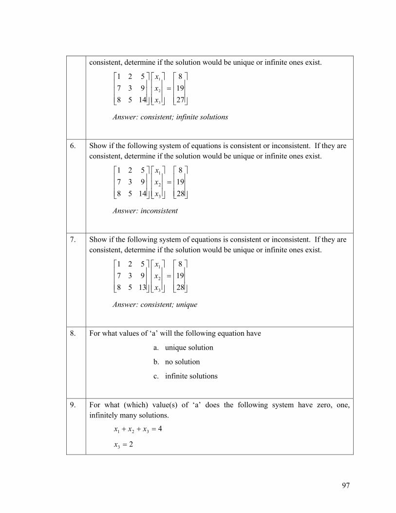
consistent, determine if the solution would be unique or infinite ones exist.
⎥⎥⎥
⎦
⎤
⎢⎢⎢
⎣
⎡=
⎥⎥⎥
⎦
⎤
⎢⎢⎢
⎣
⎡
⎥⎥⎥
⎦
⎤
⎢⎢⎢
⎣
⎡
27198
1458937521
3
2
1
xxx
Answer: consistent; infinite solutions
6. Show if the following system of equations is consistent or inconsistent. If they are consistent, determine if the solution would be unique or infinite ones exist.
⎥⎥⎥
⎦
⎤
⎢⎢⎢
⎣
⎡=
⎥⎥⎥
⎦
⎤
⎢⎢⎢
⎣
⎡
⎥⎥⎥
⎦
⎤
⎢⎢⎢
⎣
⎡
28198
1458937521
3
2
1
xxx
Answer: inconsistent
7. Show if the following system of equations is consistent or inconsistent. If they are consistent, determine if the solution would be unique or infinite ones exist.
⎥⎥⎥
⎦
⎤
⎢⎢⎢
⎣
⎡=
⎥⎥⎥
⎦
⎤
⎢⎢⎢
⎣
⎡
⎥⎥⎥
⎦
⎤
⎢⎢⎢
⎣
⎡
28198
1358937521
3
2
1
xxx
Answer: consistent; unique
8. For what values of ‘a’ will the following equation have
a. unique solution
b. no solution
c. infinite solutions
9. For what (which) value(s) of ‘a’ does the following system have zero, one, infinitely many solutions.
4
2
321 =++ xxx
3 =x
97

( ) 24 312 −=+− axxa
Answer: if ,2 2 −+≠ ora then there will be a unique solution
if then there will be no solution. 2,-or 2+=a
Possibility of infinite solutions does not exist.
10. Find if
⎥⎦
⎤⎢⎣
⎡=⎥
⎦
⎤⎢⎣
⎡−
−=
5.02.025.03.0
][32
5.25][ BandA
are inverse of each other.
Answer: Yes
11.
Find if
⎥⎦
⎤⎢⎣
⎡ −=⎥
⎦
⎤⎢⎣
⎡=
5.02.025.03.0
][325.25
][ BandA
are inverse of each other.
Answer: No
12. Find the
a. cofactor matrix
b. adjoint matrix
of
[ ]⎥⎥⎥
⎦
⎤
⎢⎢⎢
⎣
⎡−−=518172
143A
13. Find [A]-1 using any method
98

⎥⎥⎥
⎦
⎤
⎢⎢⎢
⎣
⎡−−=518172
143 [A]
Answer: [ ]⎥⎥⎥
⎦
⎤
⎢⎢⎢
⎣
⎡
−−−−−
=−−−
−−−
−−−
−
111
221
211
1
2.500x102.500x105.000x104.310x106.034x101.552x102.586x101.638x102.931x10
A
14.
Prove that if [A] and [B] are both invertible and are square matrices of same order, then
([A][B]) =[B] [A] 1− 1− 1−
Hint:
[ ][ ]( ) [ ] [ ] 111 −−− = ABBA
Let [ ] [ ][ ]BAC =
[ ][ ] [ ][ ][ ] 11 −− = BBABC
[ ][ ]IA=
[ ]A=
Again [ ] [ ][ ]BAC =
[ ] [ ] [ ] [ ][ ]BAACA 11 −− =
[ ][ ]BI=
[ ]B=
So
[ ][ ] [ ] ( )[ ] [ ] [ ] ( )2
11
1
−−−−−=
−−−−−=−
−
BCA
ABC
99

From (1) and (2)
[ ][ ] [ ] [ ] [ ][ ]BACABC =−− 11
[ ][ ][ ] [ ] [ ][ ] [ ][ ]BABAABBA =−− 11
[ ] [ ][ ][ ] [ ] [ ][ ] [ ][ ][ ]BAABAABBAA 1111 −−−− =
[ ][ ] [ ][ ][ ] [ ]BBAABB =−− 11
[ ][ ][ ] [ ][ ][ ] [ ] [ ]BBBAABBB 1111 −−−− =
[ ] [ ][ ][ ] [ ].11 IBAAB =−−
15.
What is the inverse of a square diagonal matrix? Does it always exist?
Hint: Inverse of a square n×n diagonal matrix [ is ]A
[ ]
⎥⎥⎥⎥⎥⎥⎥⎥
⎦
⎤
⎢⎢⎢⎢⎢⎢⎢⎢
⎣
⎡
=−
nna
a
a
A
10
010
001
22
11
1
LLM
M
L
L
So inverse exists only if 0≠iia for all i.
16.
[A] and [B] are square matrices. If [A][B] = [0] and [A] is invertible, show[B] = 0.
Hint: [ ][ ] [ ]0=BA
[ ][ ][ ] [ ] [011 −− = ABAA ]
17.
If [A] [B] [C]=[I], where [A], [B] and [C] are of the same size,
100

show that [B] is invertible.
18.
Prove if [B] is invertible,
[A][B]-1 = [B]-1 [A] if and only if [A][B] =[B][A]
Hint: Multiply by [ ] 1−B on both sides,
[ ][ ][ ] [ ] [ ][ ] 111 −−− = BABBBA
19.
For
[ ]⎥⎥⎥
⎦
⎤
⎢⎢⎢
⎣
⎡
−−
−=
5156099.230710
A
[ ]⎥⎥⎥
⎦
⎤
⎢⎢⎢
⎣
⎡
×−−−−
=−
−
5
1
10664.61666.004995.03999.03332.02999.02799.02333.01099.0
A
Show ( ) ( ).det1det 1−=A
A
20. For what values of ‘a’ does the linear system have
x + y= 2
6x + 6 y = a
a) infinite solutions _________________________
b) unique solution _ ______________
Answer: a) 12 b) not possible
21. Three kids - Jim, Corey and David receive an inheritance of $2,253,453. The money is put in three trusts but is not divided equally to begin with. Corey
101
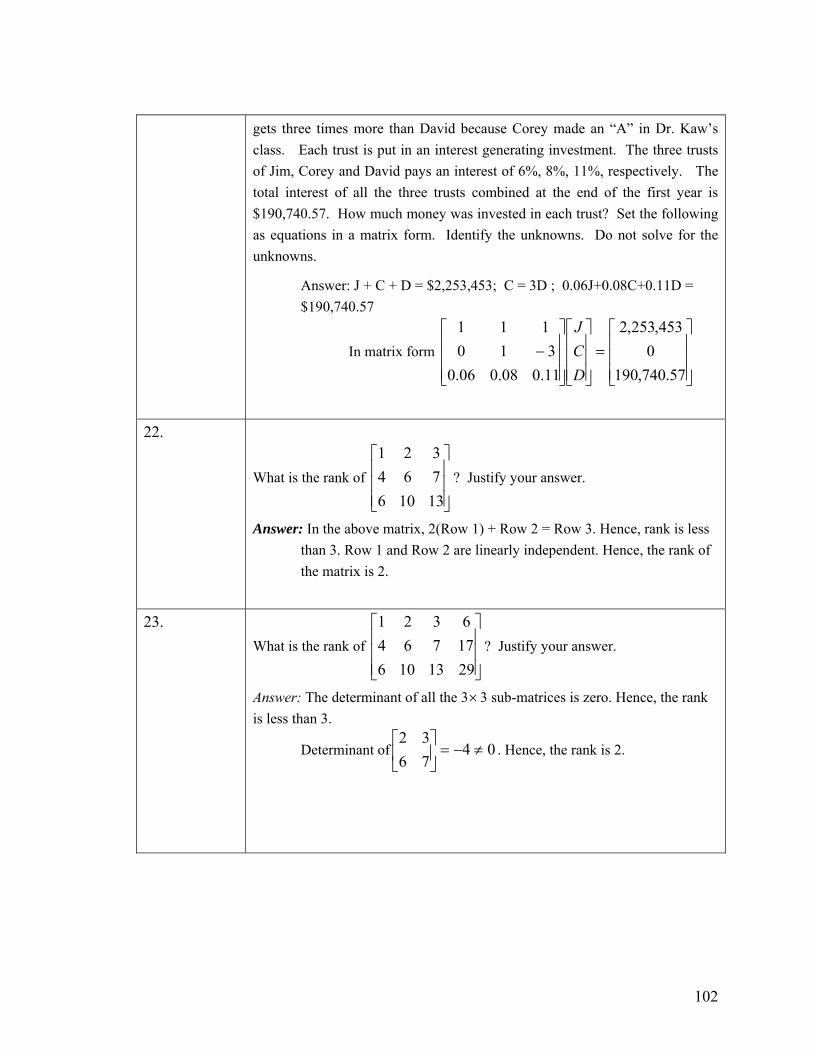
gets three times more than David because Corey made an “A” in Dr. Kaw’s class. Each trust is put in an interest generating investment. The three trusts of Jim, Corey and David pays an interest of 6%, 8%, 11%, respectively. The total interest of all the three trusts combined at the end of the first year is $190,740.57. How much money was invested in each trust? Set the following as equations in a matrix form. Identify the unknowns. Do not solve for the unknowns.
Answer: J + C + D = $2,253,453; C = 3D ; 0.06J+0.08C+0.11D = $190,740.57
In matrix form ⎥⎥⎥
⎦
⎤
⎢⎢⎢
⎣
⎡=
⎥⎥⎥
⎦
⎤
⎢⎢⎢
⎣
⎡
⎥⎥⎥
⎦
⎤
⎢⎢⎢
⎣
⎡−
57.740,1900
453,253,2
11.008.006.0310
111
DCJ
22.
What is the rank of ? Justify your answer. ⎥⎥⎥
⎦
⎤
⎢⎢⎢
⎣
⎡
13106764321
Answer: In the above matrix, 2(Row 1) + Row 2 = Row 3. Hence, rank is less than 3. Row 1 and Row 2 are linearly independent. Hence, the rank of the matrix is 2.
What is the rank of ? Justify your answer. ⎥⎥⎥
⎦
⎤
⎢⎢⎢
⎣
⎡
291310617764632123.
Answer: The determinant of all the 3×3 sub-matrices is zero. Hence, the rank is less than 3.
Determinant of . Hence, the rank is 2. 047632
≠−=⎥⎦
⎤⎢⎣
⎡
102
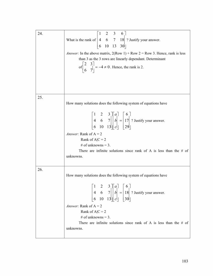
What is the rank of ? Justify your answer. ⎥⎥⎥
⎦
⎤
⎢⎢⎢
⎣
⎡
301310618764632124.
Answer: In the above matrix, 2(Row 1) + Row 2 = Row 3. Hence, rank is less than 3 as the 3 rows are linearly dependant. Determinant
of . Hence, the rank is 2. 047632
≠−=⎥⎦
⎤⎢⎣
⎡
25. How many solutions does the following system of equations have
? Justify your answer. ⎥⎥⎥
⎦
⎤
⎢⎢⎢
⎣
⎡=
⎥⎥⎥
⎦
⎤
⎢⎢⎢
⎣
⎡
⎥⎥⎥
⎦
⎤
⎢⎢⎢
⎣
⎡
29176
13106764321
cba
Answer: Rank of A = 2 Rank of A|C = 2 # of unknowns = 3. There are infinite solutions since rank of A is less than the # of unknowns.
26. How many solutions does the following system of equations have
? Justify your answer. ⎥⎥⎥
⎦
⎤
⎢⎢⎢
⎣
⎡=
⎥⎥⎥
⎦
⎤
⎢⎢⎢
⎣
⎡
⎥⎥⎥
⎦
⎤
⎢⎢⎢
⎣
⎡
30186
13106764321
cba
Answer: Rank of A = 2 Rank of A|C = 2 # of unknowns = 3. There are infinite solutions since rank of A is less than the # of unknowns.
103
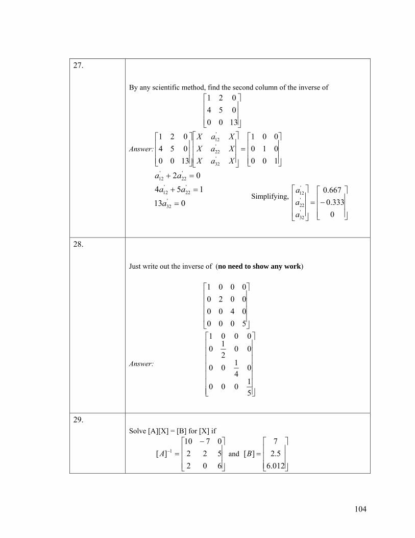
27.
By any scientific method, find the second column of the inverse of
⎥⎥⎥
⎦
⎤
⎢⎢⎢
⎣
⎡
1300054021
Answer: ⎥⎥⎥
⎦
⎤
⎢⎢⎢
⎣
⎡=
⎥⎥⎥
⎦
⎤
⎢⎢⎢
⎣
⎡
⎥⎥⎥
⎦
⎤
⎢⎢⎢
⎣
⎡
100010001
1300054021
'32
'22
'12
XaXXaXXaX
Simplifying, 013
154
02
'32
'22
'12
'22
'12
=
=+
=+
a
aa
aa
⎥⎥⎥
⎦
⎤
⎢⎢⎢
⎣
⎡−=
⎥⎥⎥
⎦
⎤
⎢⎢⎢
⎣
⎡
0333.0
667.0
'32
'22
'12
aaa
28. Just write out the inverse of (no need to show any work)
⎥⎥⎥⎥
⎦
⎤
⎢⎢⎢⎢
⎣
⎡
5000040000200001
Answer:
⎥⎥⎥⎥⎥⎥⎥
⎦
⎤
⎢⎢⎢⎢⎢⎢⎢
⎣
⎡
51000
04100
00210
0001
29. Solve [A][X] = [B] for [X] if
and ⎥⎥⎥
⎦
⎤
⎢⎢⎢
⎣
⎡ −=−
6025220710
][ 1A⎥⎥⎥
⎦
⎤
⎢⎢⎢
⎣
⎡=
012.65.2
7][B
104
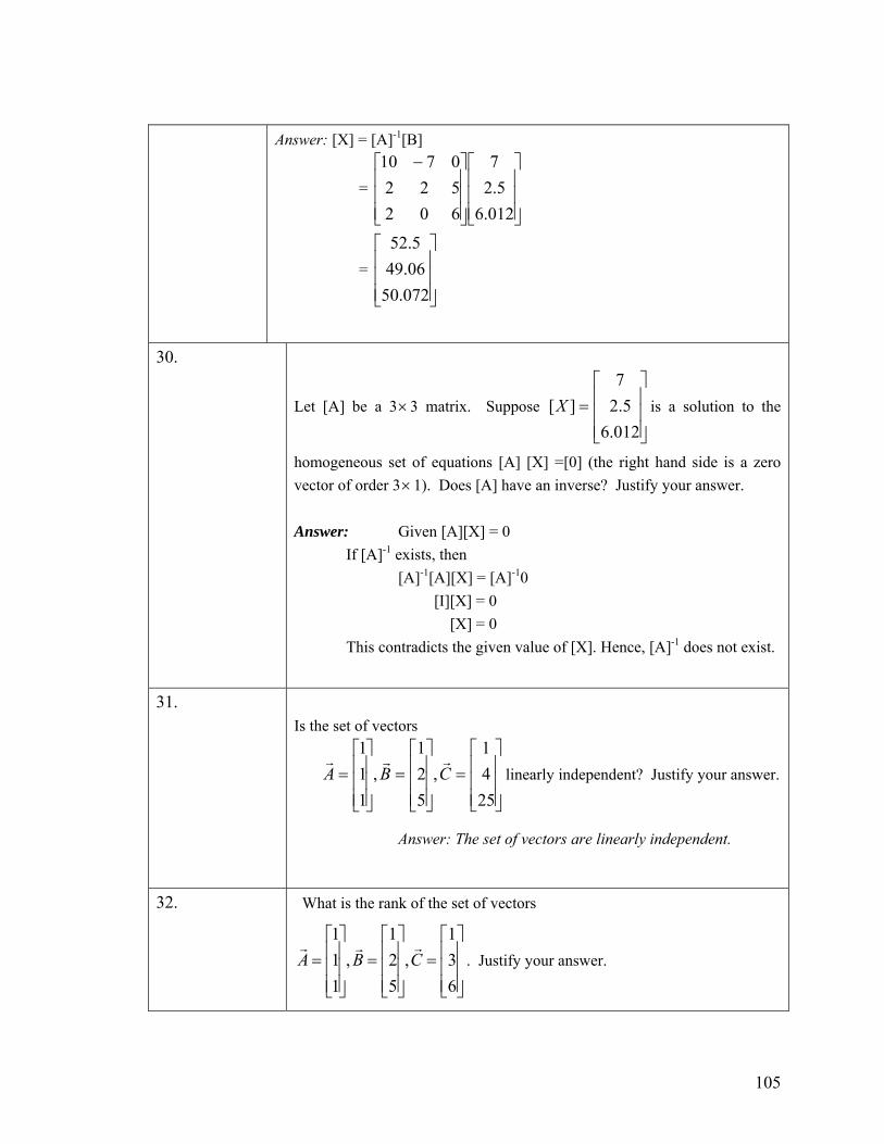
Answer: [X] = [A]-1[B]
= ⎥⎥⎥
⎦
⎤
⎢⎢⎢
⎣
⎡
⎥⎥⎥
⎦
⎤
⎢⎢⎢
⎣
⎡ −
012.65.2
7
6025220710
= ⎥⎥⎥
⎦
⎤
⎢⎢⎢
⎣
⎡
072.5006.495.52
30.
Let [A] be a 3×3 matrix. Suppose is a solution to the
homogeneous set of equations [A] [X] =[0] (the right hand side is a zero vector of order 3
⎥⎥⎥
⎦
⎤
⎢⎢⎢
⎣
⎡=
012.65.2
7][X
×1). Does [A] have an inverse? Justify your answer. Answer: Given [A][X] = 0 If [A]-1 exists, then [A]-1[A][X] = [A]-10 [I][X] = 0 [X] = 0 This contradicts the given value of [X]. Hence, [A]-1 does not exist.
31. Is the set of vectors
⎥⎥⎥
⎦
⎤
⎢⎢⎢
⎣
⎡=
⎥⎥⎥
⎦
⎤
⎢⎢⎢
⎣
⎡=
⎥⎥⎥
⎦
⎤
⎢⎢⎢
⎣
⎡=
2541
,521
,111
CBArrr
linearly independent? Justify your answer.
Answer: The set of vectors are linearly independent.
32. What is the rank of the set of vectors
⎥⎥⎥
⎦
⎤
⎢⎢⎢
⎣
⎡=
⎥⎥⎥
⎦
⎤
⎢⎢⎢
⎣
⎡=
⎥⎥⎥
⎦
⎤
⎢⎢⎢
⎣
⎡=
631
,521
,111
CBArrr
. Justify your answer.
105
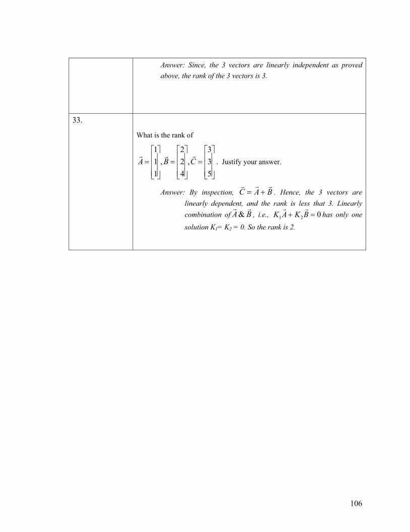
Answer: Since, the 3 vectors are linearly independent as proved above, the rank of the 3 vectors is 3.
33.
What is the rank of
⎥⎥⎥
⎦
⎤
⎢⎢⎢
⎣
⎡=
⎥⎥⎥
⎦
⎤
⎢⎢⎢
⎣
⎡=
⎥⎥⎥
⎦
⎤
⎢⎢⎢
⎣
⎡=
533
,422
,111
CBArrr
. Justify your answer.
Answer: By inspection, BACrrv
+= . Hence, the 3 vectors are linearly dependent, and the rank is less that 3. Linearly combination of BA
rr& , i.e., 021 =+ BKAK
rrhas only one
solution K1= K2 = 0. So the rank is 2.
106
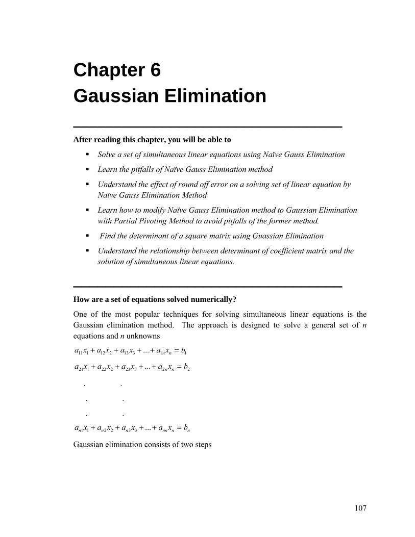
Chapter 6 Gaussian Elimination _________________________________
After reading this chapter, you will be able to
Solve a set of simultaneous linear equations using Naïve Gauss Elimination
Learn the pitfalls of Naïve Gauss Elimination method
Understand the effect of round off error on a solving set of linear equation by Naïve Gauss Elimination Method
Learn how to modify Naïve Gauss Elimination method to Gaussian Elimination with Partial Pivoting Method to avoid pitfalls of the former method.
Find the determinant of a square matrix using Guassian Elimination
Understand the relationship between determinant of coefficient matrix and the solution of simultaneous linear equations.
_________________________________
How are a set of equations solved numerically?
One of the most popular techniques for solving simultaneous linear equations is the Gaussian elimination method. The approach is designed to solve a general set of n equations and n unknowns
11313212111 ... bxaxaxaxa nn =++++
22323222121 ... bxaxaxaxa nn =++++
. .
. .
. .
nnnnnnn bxaxaxaxa =++++ ...332211
Gaussian elimination consists of two steps
107

1. Forward Elimination of Unknowns: In this step, the unknown is eliminated in each equation starting with the first equation. This way, the equations are “reduced” to one equation and one unknown in each equation.
2. Back Substitution: In this step, starting from the last equation, each of the unknowns is found.
Forward Elimination of Unknowns: In the first step of forward elimination, the first unknown, x1 is eliminated from all rows below the first row. The first equation is selected as the pivot equation to eliminate x1. So, to eliminate x1 in the second equation, one divides the first equation by a11 (hence called the pivot element) and then multiply it by a21. That is, same as multiplying the first equation by a21/ a11 to give
111
211
11
21212
11
21121 ... b
aaxa
aaxa
aaxa nn =+++
Now, this equation can be subtracted from the second equation to give
111
2121
11
212212
11
2122 ... b
aabxa
aaaxa
aaa nnn −=⎟⎟
⎠
⎞⎜⎜⎝
⎛−++⎟⎟
⎠
⎞⎜⎜⎝
⎛−
or '2
'22
'22 ... bxaxa nn =++
where
nnn aaaaa
aaaaa
111
212
'2
1211
2122
'22
−=
−=
M
This procedure of eliminating , is now repeated for the third equation to the n1x th equation to reduce the set of equations as
11313212111 ... bxaxaxaxa nn =++++
'2
'23
'232
'22 ... bxaxaxa nn =+++
'3
'33
'332
'32 ... bxaxaxa nn =+++
. . .
. . .
. . .
108
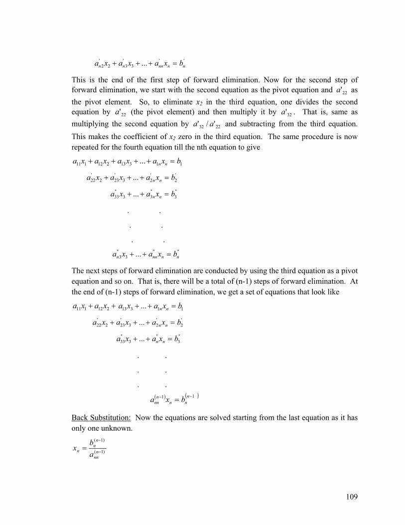
''3
'32
'2 ... nnnnnn bxaxaxa =+++
This is the end of the first step of forward elimination. Now for the second step of forward elimination, we start with the second equation as the pivot equation and as the pivot element. So, to eliminate x
22'a2 in the third equation, one divides the second
equation by (the pivot element) and then multiply it by . That is, same as multiplying the second equation by and subtracting from the third equation. This makes the coefficient of x
22'a 32'a
2232 '/' aa
2 zero in the third equation. The same procedure is now repeated for the fourth equation till the nth equation to give
11313212111 ... bxaxaxaxa nn =++++
'2
'23
'232
'22 ... bxaxaxa nn =+++
"3
"33
"33 ... bxaxa nn =++
. .
. .
. .
""3
"3 ... nnnnn bxaxa =++
The next steps of forward elimination are conducted by using the third equation as a pivot equation and so on. That is, there will be a total of (n-1) steps of forward elimination. At the end of (n-1) steps of forward elimination, we get a set of equations that look like
++ 212111 xaxa 11313 ... bxaxa nn =++
'2
'23
'232
'22 ... bxaxaxa nn =+++
"3
"3
"33 ... bxaxa nn =++
. .
. .
. .
( ) ( )11 −− = nnn
nnn bxa
Back Substitution: Now the equations are solved starting from the last equation as it has only one unknown.
)1(
)1(
−
−
= nnn
nn
n ab
x
109

Then the second last equation, that is the (n-1)th equation, has two unknowns - xn and xn-1, but xn is already known. This reduces the (n-1)th equation also to one unknown. Back substitution hence can be represented for all equations by the formula
( ) ( )
( )11
11
−+=
−− ∑−= i
ii
n
ijj
iij
ii
i a
xabx for i = n – 1, n – 2,…,1
and
)1(
)1(
−
−
= nnn
nn
n ab
x
_________________________________ Example
The upward velocity of a rocket is given at three different times in the following table
Time, t Velocity, v
s m/s
5 106.8
8 177.2
12 279.2
The velocity data is approximated by a polynomial as
( ) 12.t5 , 322
1 ≤≤++= atatatv
The coefficients for the above expression were found in Chapter 5 to be given by
321 , a, aa
⎥⎥⎥
⎦
⎤
⎢⎢⎢
⎣
⎡=
⎥⎥⎥
⎦
⎤
⎢⎢⎢
⎣
⎡
⎥⎥⎥
⎦
⎤
⎢⎢⎢
⎣
⎡
2.2792.1778.106
aaa
11214418641525
3
2
1
Find the values of a1, a2, a3 using Naïve Guass Elimination. Find the velocity at seconds. 11 ,9 ,5.7 ,6=t
Solution
110
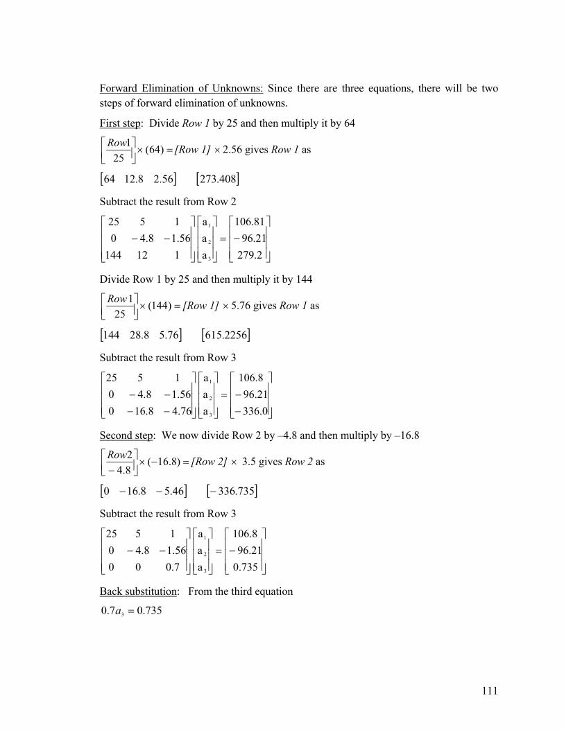
Forward Elimination of Unknowns: Since there are three equations, there will be two steps of forward elimination of unknowns.
First step: Divide Row 1 by 25 and then multiply it by 64
=×⎥⎦⎤
⎢⎣⎡ )64(
251Row [Row 1] 2.56 gives Row 1 as ×
[ ] [ 408.27356.28.1264 ] Subtract the result from Row 2
⎥⎥⎥
⎦
⎤
⎢⎢⎢
⎣
⎡−=
⎥⎥⎥
⎦
⎤
⎢⎢⎢
⎣
⎡
⎥⎥⎥
⎦
⎤
⎢⎢⎢
⎣
⎡−−
2.27921.9681.106
aaa
11214456.18.40
1525
3
2
1
Divide Row 1 by 25 and then multiply it by 144
=×⎥⎦⎤
⎢⎣⎡ )144(
251 Row [Row 1] 5.76 gives Row 1 as ×
[ ] [ 2256.61576.58.28144 ] Subtract the result from Row 3
⎥⎥⎥
⎦
⎤
⎢⎢⎢
⎣
⎡
−−=
⎥⎥⎥
⎦
⎤
⎢⎢⎢
⎣
⎡
⎥⎥⎥
⎦
⎤
⎢⎢⎢
⎣
⎡
−−−−
0.33621.968.106
aaa
76.48.16056.18.40
1525
3
2
1
Second step: We now divide Row 2 by –4.8 and then multiply by –16.8
=−×⎥⎦⎤
⎢⎣⎡−
)8.16(8.42Row [Row 2] × 3.5 gives Row 2 as
[ ] [ 735.33646.58.160 −−− ] Subtract the result from Row 3
⎥⎥⎥
⎦
⎤
⎢⎢⎢
⎣
⎡−=
⎥⎥⎥
⎦
⎤
⎢⎢⎢
⎣
⎡
⎥⎥⎥
⎦
⎤
⎢⎢⎢
⎣
⎡−−
735.021.968.106
aaa
7.00056.18.40
1525
3
2
1
Back substitution: From the third equation
735.07.0 3 =a
111

0.70.735a 3 =
1.050 =
Substituting the value of a3 in the second equation,
21.9656.18.4 32 −=−− aa
8.456.121.96 3
2 −+−
=a
a
( )4.8-
1.0501.5696.21- +=
7019. =
Substituting the value of in the first equation, 32 and aa
8.106525 321 =++ aaa
2558.106
321
aaa
−−=
( )25
050.170.1958.106 −−=
2900.0 =
Hence the solution vector is
⎥⎥⎥
⎦
⎤
⎢⎢⎢
⎣
⎡=
⎥⎥⎥
⎦
⎤
⎢⎢⎢
⎣
⎡
050.170.19
2900.0
3
2
1
aaa
The polynomial that passes through the three data points is then
( ) 322
1 atatatv ++=
125 ,050.170.192900.0 2 ≤≤++= ttt
Since we want to find the velocity at 11 and 9 ,5.7 ,6=t seconds, we could simply substitute each value of t in ( ) 050.170.192900.0 2 ++= tttv and find the corresponding velocity. For example, at 6=t
( ) ( ) ( )./ 69.129
050.1670.1962900.06 2
smv
=++=
112

However we could also find all the needed values of velocity at t = 6, 7.5, 9 and 11 seconds using matrix multiplication.
( ) [ ]⎥⎥⎥
⎦
⎤
⎢⎢⎢
⎣
⎡
=1
1.05 19.7 29.0
2
tt
tv
So if we want to find ( ) ( ) ( ) ( ),11 ,9 ,5.7 ,6 vvvv it is given by
( ) ( ) ( ) ( )[ ]11 9 5.7 6 vvvv
[ ]⎥⎥⎥
⎦
⎤
⎢⎢⎢
⎣
⎡
=11111195.76
1195.76 05.1 7.19 0.29
2222
[ ]⎥⎥⎥
⎦
⎤
⎢⎢⎢
⎣
⎡=
11111197.561218156.2536
1.050 19.70 2900.0
[ ]252.8 201.8 165.1 7.129 =
( ) smv / 7.1296 =
( ) smv / 1.1655.7 =
( ) smv / 8.2019 =
( ) smv / 8.25211 =
_________________________________ Example
Use Naïve Gauss Elimination to solve
7710 21 =− xx
901.36099.23 321 =++− xxx
655 321 =+− xxx
Use six significant digits with chopping in your calculations.
Solution
Working in the matrix form
113

⎥⎥⎥
⎦
⎤
⎢⎢⎢
⎣
⎡
−−
−
5156099.230710
⎥⎥⎥
⎦
⎤
⎢⎢⎢
⎣
⎡
3
2
1
xxx
= ⎥⎥⎥
⎦
⎤
⎢⎢⎢
⎣
⎡
6901.37
Forward Elimination of Unknowns
Dividing Row 1 by 10 and multiplying by –3, that is, multiplying Row 1 by -0.3, and subtract it from Row 2 would eliminate a21,
⎥⎥⎥
⎦
⎤
⎢⎢⎢
⎣
⎡
−−−
5156001.000710
⎥⎥⎥
⎦
⎤
⎢⎢⎢
⎣
⎡
3
2
1
xxx
= ⎥⎥⎥
⎦
⎤
⎢⎢⎢
⎣
⎡
6001.67
Again dividing Row 1 by 10 and multiplying by 5, that is, multiplying Row 1 by 0.5, and subtract it from Row 3 would eliminate a31,
⎥⎥⎥
⎦
⎤
⎢⎢⎢
⎣
⎡−−
55.206001.000710
⎥⎥⎥
⎦
⎤
⎢⎢⎢
⎣
⎡
3
2
1
xxx
=
⎥⎥⎥
⎦
⎤
⎢⎢⎢
⎣
⎡
5.2001.67
This is the end of the first step of forward elimination.
Now for the second step of forward elimination, we would use Row 2 as the pivot equation and eliminate Row 3 – Column 2. Dividing Row 2 by –0.001 and multiplying by 2.5, that is multiplying Row 2 by –2500, and subtracting from Row 3 gives
⎥⎥⎥
⎦
⎤
⎢⎢⎢
⎣
⎡−−
15005006001.000710
= ⎥⎥⎥
⎦
⎤
⎢⎢⎢
⎣
⎡
3
2
1
xxx
⎥⎥⎥
⎦
⎤
⎢⎢⎢
⎣
⎡
15005001.67
This is the end of the forward elimination steps.
Back substitution
We can now solve the above equations by back substitution. From the third equation,
1500515005 3 =x
1500515005
3 =x
.1=
Substituting the value of x3 in the second equation
001.66001.0 32 =+− xx
114
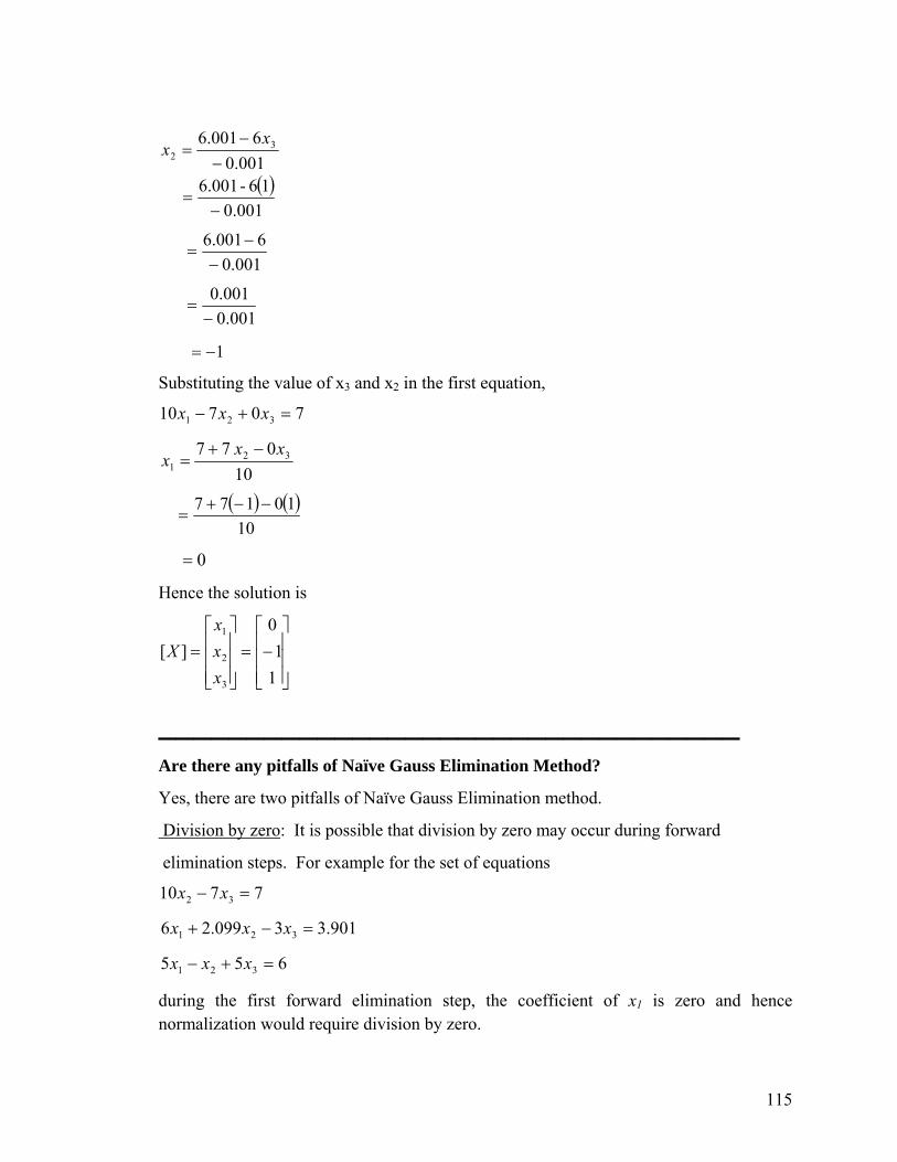
( )001.0
16-6.001
001.06001.6 3
2
−=
−−
=x
x
001.0
6001.6−
−=
001.0
001.0−
=
1−=
Substituting the value of x3 and x2 in the first equation,
70710 321 =+− xxx
100 77 32
1xx
x−+
=
( ) ( )10
10177 −−+=
0 =
Hence the solution is
⎥⎥⎥
⎦
⎤
⎢⎢⎢
⎣
⎡−=
⎥⎥⎥
⎦
⎤
⎢⎢⎢
⎣
⎡=
11
0][
3
2
1
xxx
X
_________________________________ Are there any pitfalls of Naïve Gauss Elimination Method?
Yes, there are two pitfalls of Naïve Gauss Elimination method.
Division by zero: It is possible that division by zero may occur during forward
elimination steps. For example for the set of equations
7
6
710 32 =− xx
901.33099.26 321 =−+ xxx
55 321 =+− xxx
during the first forward elimination step, the coefficient of x1 is zero and hence normalization would require division by zero.
115

Round-off error: Naïve Gauss Elimination Method is prone to round-off errors. This is true when there are large numbers of equations as errors propagate. Also, if there is subtraction of numbers from each other, it may create large errors. See the example below.
_________________________________ Example
Remember the previous example where we used Naïve Gauss Elimination to solve
7710 21 =− xx
901.36099.23 321 =++− xxx
655 321 =+− xxx
using six significant digits with chopping in your calculations. Repeat the problem, but now use five significant digits with chopping in your calculations.
Solution
Writing in the matrix form
⎥⎥⎥
⎦
⎤
⎢⎢⎢
⎣
⎡
−−
−
5156099.230710
= ⎥⎥⎥
⎦
⎤
⎢⎢⎢
⎣
⎡
3
2
1
xxx
⎥⎥⎥
⎦
⎤
⎢⎢⎢
⎣
⎡
6901.37
Forward Elimination of Unknowns
Dividing Row 1 by 10 and multiplying by –3, that is, multiplying Row 1 by -0.3, and subtract it from Row 2 would eliminate a21,
⎥⎥⎥
⎦
⎤
⎢⎢⎢
⎣
⎡
−−−
5156001.000710
⎥⎥⎥
⎦
⎤
⎢⎢⎢
⎣
⎡
3
2
1
xxx
= ⎥⎥⎥
⎦
⎤
⎢⎢⎢
⎣
⎡
6001.67
Again dividing Row 1 by 10 and multiplying by 5, that is, multiplying the Row 1 by 0.5, and subtract it from Row 3 would eliminate a31,
=
⎥⎥⎥
⎦
⎤
⎢⎢⎢
⎣
⎡−−
55.206001.000710
⎥⎥⎥
⎦
⎤
⎢⎢⎢
⎣
⎡
3
2
1
xxx
⎥⎥⎥
⎦
⎤
⎢⎢⎢
⎣
⎡
5.2001.67
This is the end of the first step of forward elimination.
116

Now for the second step of forward elimination, we would use Row 2 as the pivoting equation and eliminate Row 3 – Column 2. Dividing Row 2 by –0.001 and multiplying by 2.5, that is, multiplying Row 2 by –2500, and subtract from Row 3 gives
⎥⎥⎥
⎦
⎤
⎢⎢⎢
⎣
⎡−−
15005006001.000710
⎥⎥⎥
⎦
⎤
⎢⎢⎢
⎣
⎡
3
2
1
xxx
= ⎥⎥⎥
⎦
⎤
⎢⎢⎢
⎣
⎡
15004001.67
This is the end of the forward elimination steps.
Back substitution
We can now solve the above equations by back substitution. From the third equation,
1500415005 3 =x
1500515004
3 =x
99993.0=
Substituting the value of x3 in the second equation
001.66001.0 32 =+− xx
( )
0.001-5.9995-6.001
0.001-0.999936-6.001
001.06001.6 3
2
=
=
−−
=x
x
001.0
0015.0−
=
5.1−=
Substituting the value of x3 and x2 in the first equation,
70710 321 =+− xxx
10077 32
1xx
x−+
=
( ) ( )10
105.177 −−+=
117

=10
05.107 −−
=10
5.3−
= 3500.0−
Hence the solution is
[ ]⎥⎥⎥
⎦
⎤
⎢⎢⎢
⎣
⎡=
3
2
1
xxx
X
⎥⎥⎥
⎦
⎤
⎢⎢⎢
⎣
⎡−−
=99993.0
5.135.0
Compare this with the exact solution of
[ ]⎥⎥⎥
⎦
⎤
⎢⎢⎢
⎣
⎡=
3
2
1
xxx
X
⎥⎥⎥
⎦
⎤
⎢⎢⎢
⎣
⎡−=11
0
_________________________________ What are the techniques for improving Naïve Gauss Elimination Method?
As seen in the example, round off errors were large when five significant digits were used as opposed to six significant digits. So one way of decreasing round off error would be to use more significant digits, that is, use double or quad precision. However, this would not avoid division by zero errors in Naïve Gauss Elimination. To avoid division by zero as well as reduce (not eliminate) round off error, Gaussian Elimination with partial pivoting is the method of choice.
How does Gaussian elimination with partial pivoting differ from Naïve Gauss elimination?
The two methods are the same, except in the beginning of each step of forward elimination, a row switching is done based on the following criterion. If there are n
118
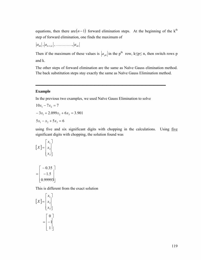
equations, then there are ( forward elimination steps. At the beginning of the k)1−n th step of forward elimination, one finds the maximum of
kka , kka ,1+ , …………, nka
Then if the maximum of these values is pka in the pth row, k≤p≤ n, then switch rows p
and k.
The other steps of forward elimination are the same as Naïve Gauss elimination method. The back substitution steps stay exactly the same as Naïve Gauss Elimination method.
_________________________________ Example
In the previous two examples, we used Naïve Gauss Elimination to solve
7710 21 =− xx
901.36099.23 321 =++− xxx
655 321 =+− xxx
using five and six significant digits with chopping in the calculations. Using five significant digits with chopping, the solution found was
[ ]⎥⎥⎥
⎦
⎤
⎢⎢⎢
⎣
⎡=
3
2
1
xxx
X
⎥⎥⎥
⎦
⎤
⎢⎢⎢
⎣
⎡−−
=99993.0
5.135.0
This is different from the exact solution
[ ]⎥⎥⎥
⎦
⎤
⎢⎢⎢
⎣
⎡=
3
2
1
xxx
X
⎥⎥⎥
⎦
⎤
⎢⎢⎢
⎣
⎡−=11
0
119
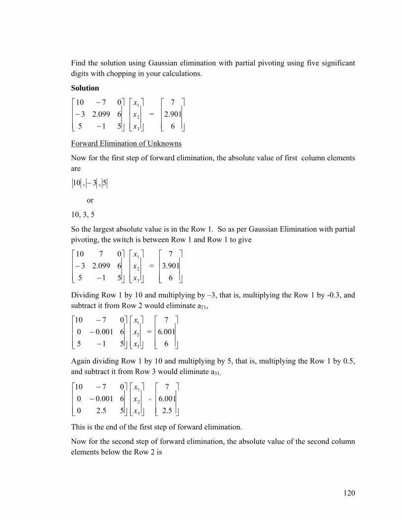
Find the solution using Gaussian elimination with partial pivoting using five significant digits with chopping in your calculations.
Solution
⎥⎥⎥
⎦
⎤
⎢⎢⎢
⎣
⎡
−−
−
5156099.230710
= ⎥⎥⎥
⎦
⎤
⎢⎢⎢
⎣
⎡
3
2
1
xxx
⎥⎥⎥
⎦
⎤
⎢⎢⎢
⎣
⎡
6901.27
Forward Elimination of Unknowns
Now for the first step of forward elimination, the absolute value of first column elements are
10 , 3− , 5
or
10, 3, 5
So the largest absolute value is in the Row 1. So as per Gaussian Elimination with partial pivoting, the switch is between Row 1 and Row 1 to give
⎥⎥⎥
⎦
⎤
⎢⎢⎢
⎣
⎡
−−
5156099.230710
= ⎥⎥⎥
⎦
⎤
⎢⎢⎢
⎣
⎡
3
2
1
xxx
⎥⎥⎥
⎦
⎤
⎢⎢⎢
⎣
⎡
6901.37
Dividing Row 1 by 10 and multiplying by –3, that is, multiplying the Row 1 by -0.3, and subtract it from Row 2 would eliminate a21,
⎥⎥⎥
⎦
⎤
⎢⎢⎢
⎣
⎡
−−−
5156001.000710
⎥⎥⎥
⎦
⎤
⎢⎢⎢
⎣
⎡
3
2
1
xxx
= ⎥⎥⎥
⎦
⎤
⎢⎢⎢
⎣
⎡
6001.67
Again dividing Row 1 by 10 and multiplying by 5, that is, multiplying the Row 1 by 0.5, and subtract it from Row 3 would eliminate a31,
⎥⎥⎥
⎦
⎤
⎢⎢⎢
⎣
⎡−−
55.206001.000710
⎥⎥⎥
⎦
⎤
⎢⎢⎢
⎣
⎡
3
2
1
xxx
=
⎥⎥⎥
⎦
⎤
⎢⎢⎢
⎣
⎡
5.2001.67
This is the end of the first step of forward elimination.
Now for the second step of forward elimination, the absolute value of the second column elements below the Row 2 is
120
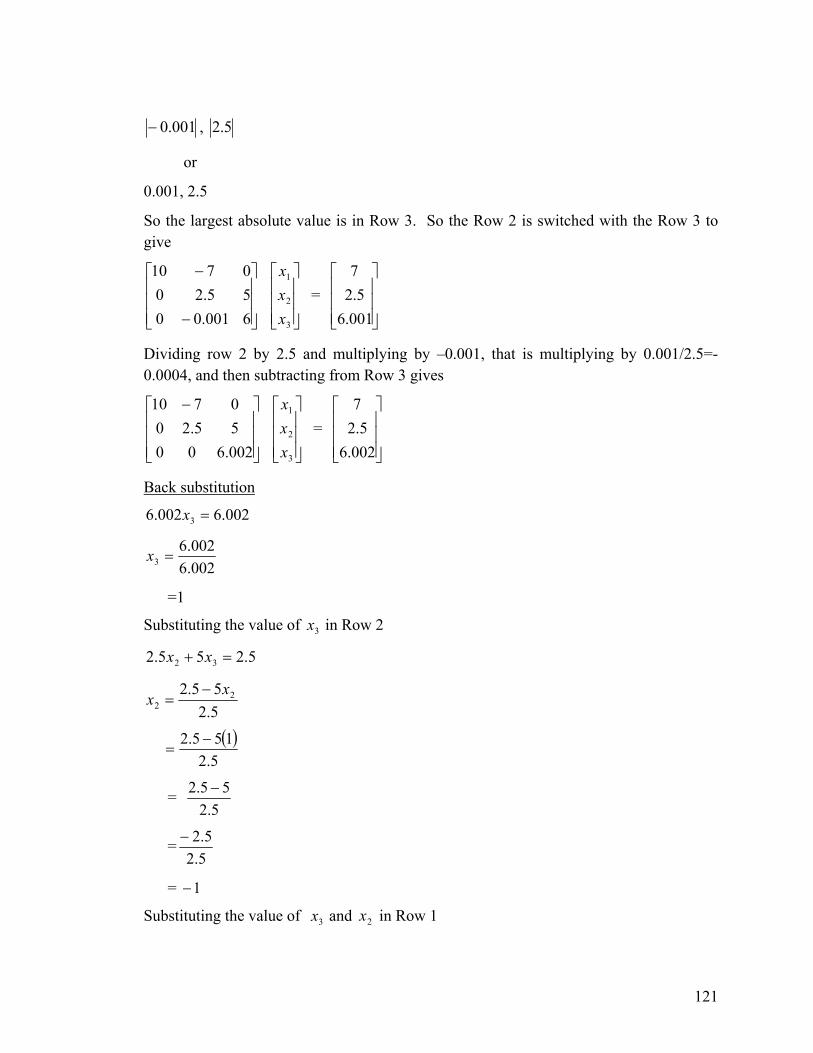
001.0− , 5.2
or
0.001, 2.5
So the largest absolute value is in Row 3. So the Row 2 is switched with the Row 3 to give
⎥⎥⎥
⎦
⎤
⎢⎢⎢
⎣
⎡
−
−
6001.0055.200710
= ⎥⎥⎥
⎦
⎤
⎢⎢⎢
⎣
⎡
3
2
1
xxx
⎥⎥⎥
⎦
⎤
⎢⎢⎢
⎣
⎡
001.65.2
7
Dividing row 2 by 2.5 and multiplying by –0.001, that is multiplying by 0.001/2.5=-0.0004, and then subtracting from Row 3 gives
⎥⎥⎥
⎦
⎤
⎢⎢⎢
⎣
⎡ −
002.60055.200710
= ⎥⎥⎥
⎦
⎤
⎢⎢⎢
⎣
⎡
3
2
1
xxx
⎥⎥⎥
⎦
⎤
⎢⎢⎢
⎣
⎡
002.65.2
7
Back substitution
002.6002.6 3 =x
002.6002.6
3 =x
=1
Substituting the value of in Row 2 3x
5.255.2 32 =+ xx
5.255.2 2
2xx −
=
( )5.2
155.2 −=
= 5.2
55.2 −
=5.25.2−
= 1−
Substituting the value of and in Row 1 3x 2x
121
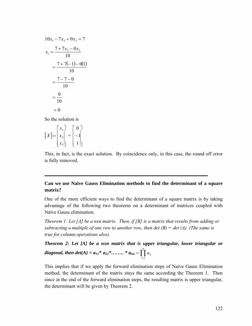
70710 221 =+− xxx
10077 32
1xxx −+
=
( ) ( )10
10177 −−+=
10077 −−
=
100 =
0 =
So the solution is
[ ]⎥⎥⎥
⎦
⎤
⎢⎢⎢
⎣
⎡=
3
2
1
xxx
X = ⎥⎥⎥
⎦
⎤
⎢⎢⎢
⎣
⎡−11
0
This, in fact, is the exact solution. By coincidence only, in this case, the round off error is fully removed.
_________________________________ Can we use Naïve Gauss Elimination methods to find the determinant of a square matrix?
One of the more efficient ways to find the determinant of a square matrix is by taking advantage of the following two theorems on a determinant of matrices coupled with Naïve Gauss elimination.
Theorem 1: Let [A] be a nxn matrix. Then, if [B] is a matrix that results from adding or subtracting a multiple of one row to another row, then det (B) = det (A). (The same is true for column operations also).
Theorem 2: Let [A] be a nxn matrix that is upper triangular, lower triangular or
diagonal, then det(A) = a11* a22*…….. * ann ∏=
=n
iiia
1
This implies that if we apply the forward elimination steps of Naive Gauss Elimination method, the determinant of the matrix stays the same according the Theorem 1. Then since at the end of the forward elimination steps, the resulting matrix is upper triangular, the determinant will be given by Theorem 2.
122

_________________________________ Example
Find the determinant of
[A]= ⎥⎥⎥
⎦
⎤
⎢⎢⎢
⎣
⎡
11214418641525
Solution
Remember earlier in this chapter, we conducted the steps of forward elimination of unknowns using Naïve Gauss Elimination method on [A] to give
[ ]⎥⎥⎥
⎦
⎤
⎢⎢⎢
⎣
⎡−−=
7.00056.18.40
1525B
According to Theorem 2
det (A) = det (B)
( )00.84
)7.0)(8.4(25−=
−=
_________________________________ What if I cannot find the determinant of the matrix using Naive Gauss Elimination method, for example, if I get division by zero problems during Naïve Gauss Elimination method?
Well, you can apply Gaussian Elimination with partial pivoting. However, the determinant of the resulting upper triangular matrix may differ by a sign. The following theorem applies in addition to the previous two to find determinant of a square matrix.
Theorem 3: Let [A] be a nxn matrix. Then, if [B] is a matrix that results from switching one row with another row, then det (B) = - det (A).
_________________________________ Example
Find the determinant of
123

[ ]⎥⎥⎥
⎦
⎤
⎢⎢⎢
⎣
⎡
−−
−=
5156099.230710
A
Remember from that at the end of the forward elimination steps of Gaussian elimination with partial pivoting, we obtained
[ ]⎥⎥⎥
⎦
⎤
⎢⎢⎢
⎣
⎡ −=
002.60055.200710
B
( ) 05.150)002.6)(5.2)(10(det ==B
Since rows were switched once during the forward elimination steps of Gaussian elimination with partial pivoting,
( ) )B(detAdet −=
05.150−= .
Prove det (A) = ( )1Adet1
−.
Proof
[A][A]-1 = [I]
( ) ( )( ) ( )( ) ( ).det
1det
1detdetdet det
1
1
1
−
−
−
=
=
=
AA
AAIAA
If [A] is a nxn matrix and det (A) ≠ 0, what other statements are equivalent to it?
1. [A] is invertible.
2. [A]-1 exists.
3. [A] [X] = [C] has a unique solution.
4. [A] [X] = [0] solution is [X] = 0r
.
5. [A] [A]-1 = [I] = [A]-1 [A].
Key Terms
Naïve Gauss Elimination Partial Pivoting Determinant
124
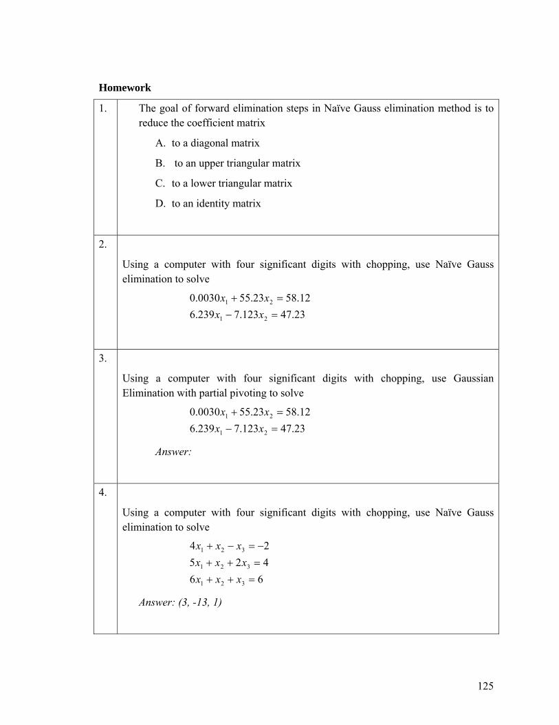
Homework
1. The goal of forward elimination steps in Naïve Gauss elimination method is to reduce the coefficient matrix
A. to a diagonal matrix
B. to an upper triangular matrix
C. to a lower triangular matrix
D. to an identity matrix
2.
Using a computer with four significant digits with chopping, use Naïve Gauss elimination to solve
23.47123.7239.612.5823.550030.0
21
21
=−=+
xxxx
3.
Using a computer with four significant digits with chopping, use Gaussian Elimination with partial pivoting to solve
23.47123.7239.612.5823.550030.0
21
21
=−=+
xxxx
Answer:
4.
Using a computer with four significant digits with chopping, use Naïve Gauss elimination to solve
6642524
321
321
321
=++=++−=−+
xxxxxx
xxx
Answer: (3, -13, 1)
125

Using a computer with four significant digits with chopping, use Gaussian Elimination with partial pivoting to solve
6642524
321
321
321
=++=++−=−+
xxxxxx
xxx
Answer: (2.995, -12.98, 1.001)
5.
For
[ ]⎥⎥⎥
⎦
⎤
⎢⎢⎢
⎣
⎡
−−
−=
5156099.230710
A
Find the determinant of [A] using forward elimination step of Naïve Gauss Elimination method.
Answer: -150.05
6.
One of the drawbacks of Naive-Gauss Elimination method is Answer: Division by zero.
7. Division by zero during forward elimination steps in Gaussian elimination with partial pivoting method implies the coefficient matrix [A] is
Answer: It implies that the co-efficient matrix is singular, that is, its determinant is zero and it is not invertible.
8. One of the advantages of Gaussian elimination with Partial Pivoting over Naive Guass Elimination method is
Answer: It overcomes the problem of Division by zero.
126

9. Show and explain clearly the first step of forward elimination of Naïve Gauss elimination method for
⎥⎥⎥
⎦
⎤
⎢⎢⎢
⎣
⎡=
⎥⎥⎥
⎦
⎤
⎢⎢⎢
⎣
⎡
⎥⎥⎥
⎦
⎤
⎢⎢⎢
⎣
⎡
30186
13106764321
cba
Answer: Dividing Row 1 by 1; multiplying it by 4 and subtracting the result from Row 2
⎥⎥⎥
⎦
⎤
⎢⎢⎢
⎣
⎡−=
⎥⎥⎥
⎦
⎤
⎢⎢⎢
⎣
⎡
⎥⎥⎥
⎦
⎤
⎢⎢⎢
⎣
⎡−−
306
6
13106520
321
cba
Dividing Row 1 by 1; multiplying it by 6 and subtracting the result from Row 3
⎥⎥⎥
⎦
⎤
⎢⎢⎢
⎣
⎡
−−=
⎥⎥⎥
⎦
⎤
⎢⎢⎢
⎣
⎡
⎥⎥⎥
⎦
⎤
⎢⎢⎢
⎣
⎡
−−−−
66
6
520520
321
cba
10. Show and explain clearly the first step of forward elimination of Gaussian elimination method with partial pivoting for
⎥⎥⎥
⎦
⎤
⎢⎢⎢
⎣
⎡=
⎥⎥⎥
⎦
⎤
⎢⎢⎢
⎣
⎡
⎥⎥⎥
⎦
⎤
⎢⎢⎢
⎣
⎡
30186
13106764321
cba
Answer: Comparing |a11|, |a21| and |a31| equals 1, 4, 6. Since 6 is greater, switch Row 3 and Row 1.
⎥⎥⎥
⎦
⎤
⎢⎢⎢
⎣
⎡=
⎥⎥⎥
⎦
⎤
⎢⎢⎢
⎣
⎡
⎥⎥⎥
⎦
⎤
⎢⎢⎢
⎣
⎡
61830
321764
13106
cba
Dividing Row 1 by 6; multiplying it by 4 and subtracting the result from Row 2
⎥⎥⎥
⎦
⎤
⎢⎢⎢
⎣
⎡−=
⎥⎥⎥
⎦
⎤
⎢⎢⎢
⎣
⎡
⎥⎥⎥
⎦
⎤
⎢⎢⎢
⎣
⎡−−
62
30
3213
53
2013106
cba
Dividing Row 1 by 6; multiplying it by 1 and subtracting the result from Row 3
⎥⎥⎥
⎦
⎤
⎢⎢⎢
⎣
⎡−=
⎥⎥⎥
⎦
⎤
⎢⎢⎢
⎣
⎡
⎥⎥⎥⎥
⎦
⎤
⎢⎢⎢⎢
⎣
⎡
−−
12
30
65
310
35
320
13106
cba
127
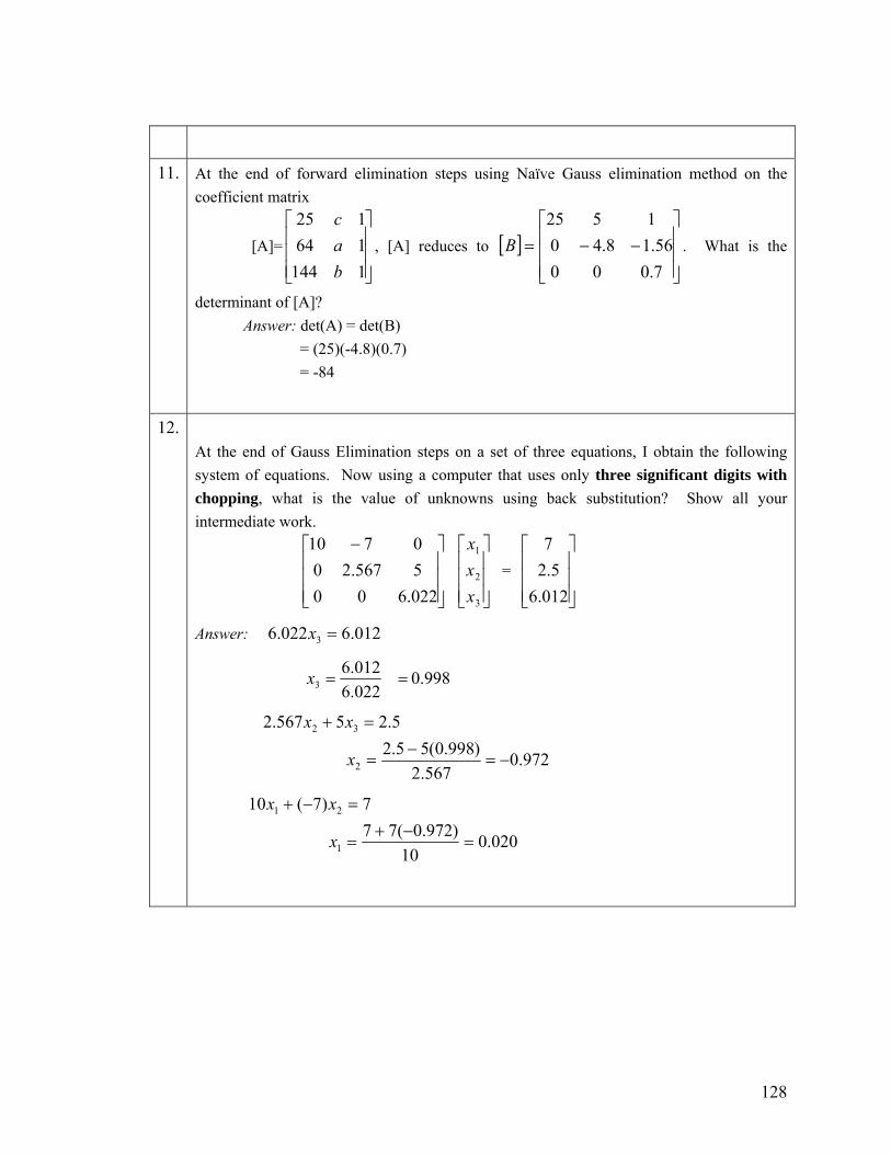
11. At the end of forward elimination steps using Naïve Gauss elimination method on the coefficient matrix
[A]= , [A] reduces to [ ] . What is the
determinant of [A]?
⎥⎥⎥
⎦
⎤
⎢⎢⎢
⎣
⎡
1144164125
bac
⎥⎥⎥
⎦
⎤
⎢⎢⎢
⎣
⎡−−=
7.00056.18.40
1525B
Answer: det(A) = det(B) = (25)(-4.8)(0.7) = -84
12. At the end of Gauss Elimination steps on a set of three equations, I obtain the following system of equations. Now using a computer that uses only three significant digits with chopping, what is the value of unknowns using back substitution? Show all your intermediate work.
⎥⎥⎥
⎦
⎤
⎢⎢⎢
⎣
⎡ −
022.6005567.200710
= ⎥⎥⎥
⎦
⎤
⎢⎢⎢
⎣
⎡
3
2
1
xxx
⎥⎥⎥
⎦
⎤
⎢⎢⎢
⎣
⎡
012.65.2
7
Answer: 012.6022.6 3 =x
0.998 022.6012.6
3 ==x
972.0
567.2)998.0(55.2
5.25567.2
2
32
−=−
=
=+
x
xx
020.0
10)972.0(77
7)7(10
1
21
=−+
=
=−+
x
xx
128

Chapter 7 LU Decomposition _________________________________ After reading this chapter, you will be able to
Learn when LU Decomposition is numerically more efficient than Gaussian Elimination
Decompose a nonsingular matrix into LU Show how LU decomposition is used to find matrix inverse.
_________________________________ I hear about LU Decomposition used as a method to solve a set of simultaneous linear equations? What is it and why do we need to learn different methods of solving a set of simultaneous linear equations?
We already studied two numerical methods of finding the solution to simultaneous linear equations – Naïve Gauss Elimination and Gaussian Elimination with Partial Pivoting. Then, why do we need to learn another method? To appreciate why LU Decomposition could be a better choice than the Gauss Elimination techniques in some cases, let us discuss first what LU Decomposition is about.
For any nonsingular matrix [ ]A on which one can conduct Naïve Gauss Elimination forward elimination steps, one can always write it as
[ ] [ ][ ]ULA =
where
[L] = lower triangular matrix
[U] = upper triangular matrix
Then if one is solving a set of equations
[A] [X] = [C],
then
129

[ ][ ][ ] [ ]CXUL = [ ][ ]( )ULA ][ =
Multiplying both side by [ ] , 1−L
[ ] [ ][ ][ ] [ ] [ ]CLXULL 11 −− =
[ ][ ][ ]XUI = [ ] [ ]CL 1− [ ] [ ]( )][1 ILL =−
[ ][ ] [ ] [ ]CLXU 1−= [ ][ ]( )][UUI =
Let
[ ] [ ] [ ]ZCL =−1
then
[ ][ ] [ ]CL =Z (1)
and
[ ][ ] [ ]ZU =X (2)
So we can solve equation (1) first for and then use equation (2) to calculate ][Z [ ]X .
This is all exciting but this looks more complicated than the Gaussian elimination techniques!! I know but I cannot tease you any longer. So here we go!
Without proof, the computational time required to decompose the matrix to [L] [U]
form is proportional to
[ ]A
3
3n , where n is the number of equations (size of matrix).
Then to solve the [ ] , the computational time is proportional to
[ ]A
[ ] [ ]CL =Z 2
2n . Then to
solve the [ ] , the computational time is proportional to [ ] [ ]CU =X 2
2n . So the total
computational time to solve a set of equations by LU decomposition is proportional to 2
3
3nn
+ .
In comparison, Gaussian elimination is computationally more efficient. It takes a
computational time proportional to 23
23 nn+ , where the computational time for forward
elimination is proportional to3
3n and for the back substitution the time is proportional
to2
2n .
130

This has confused me further! Gaussian elimination takes less time than LU Decomposition method and you are trying to convince me then LU Decomposition has its place in solving linear equations! Yes, it does.
Remember in trying to find the inverse of the matrix [ ]A in Chapter 5, the problem reduces to solving ‘n’ sets of equations with the ‘n’ columns of the identity matrix as the RHS vector. For calculations of each column of the inverse of the [ matrix, the coefficient matrix [ matrix in the set of equation
]A]A [ ][ ] [ ]CA =X does not change. So if
we use LU Decomposition method, the [ ] [ ][ ]U LA = decomposition needs to be done only once and the use of equations (1) and (2) still needs to be done ‘n’ times.
So the total computational time required to find the inverse of a matrix using LU
decomposition is proportional to 3
4)(3
32
3 nnnn=+ .
In comparison, if Gaussian elimination method were applied to find the inverse of a matrix, the time would be proportional to
2323
3423 nnnnn +=⎟⎟⎠
⎞⎜⎜⎝
⎛+ .
For large values of n
34
23
334 nnn⟩⟩+
Are you now convinced now that LU decomposition has its place in solving systems of equations? We are now ready to answer other questions - how do I find LU matrices for a nonsingular matrix [A] and how do I solve equations (1) and (2).
How do I decompose a non-singular matrix [A], that is, how do I find [ ] [ ][ ]U LA = ?
If forward elimination steps of Naïve Gauss elimination methods can be applied on a nonsingular matrix, then [ can be decomposed into L U as ]A
⎥⎥⎥⎥
⎦
⎤
⎢⎢⎢⎢
⎣
⎡
=
nnnn
n
n
aaa
aaaaaa
A
L
MLMM
L
K
21
22221
11211
][
131
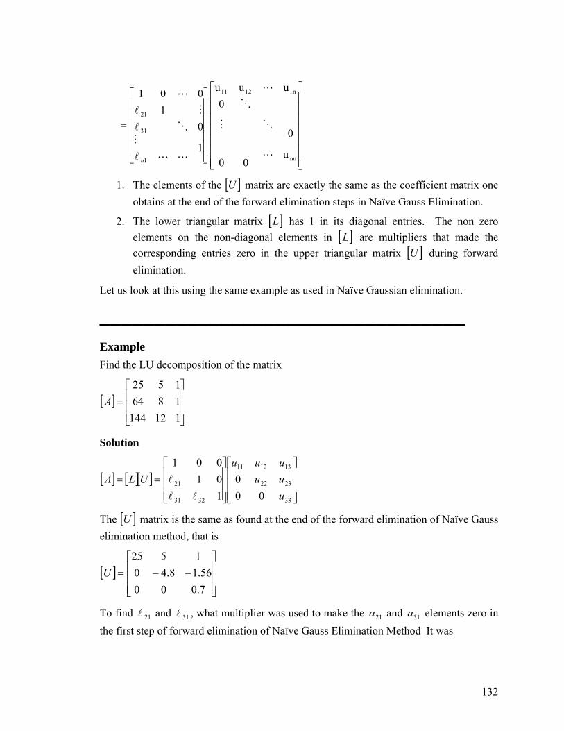
⎥⎥⎥⎥⎥⎥⎥
⎦
⎤
⎢⎢⎢⎢⎢⎢⎢
⎣
⎡
⎥⎥⎥⎥⎥⎥
⎦
⎤
⎢⎢⎢⎢⎢⎢
⎣
⎡
=
nn
1n1211
1
31
21
u00
0
0uuu
1
01
001
L
OM
O
L
LLl
MOl
Ml
L
n
1. The elements of the [ matrix are exactly the same as the coefficient matrix one obtains at the end of the forward elimination steps in Naïve Gauss Elimination.
]U
2. The lower triangular matrix [ ]L has 1 in its diagonal entries. The non zero elements on the non-diagonal elements in [ ]L are multipliers that made the corresponding entries zero in the upper triangular matrix [ during forward elimination.
]U
Let us look at this using the same example as used in Naïve Gaussian elimination.
_________________________________ Example Find the LU decomposition of the matrix
[ ]⎥⎥⎥
⎦
⎤
⎢⎢⎢
⎣
⎡=
11214418641525
A
Solution
[ ] [ ][ ]⎥⎥⎥
⎦
⎤
⎢⎢⎢
⎣
⎡
⎥⎥⎥
⎦
⎤
⎢⎢⎢
⎣
⎡==
33
2322
131211
3231
21
000
101001
uuuuuu
ULAll
l
The matrix is the same as found at the end of the forward elimination of Naïve Gauss elimination method, that is
[ ]U
[ ]⎥⎥⎥
⎦
⎤
⎢⎢⎢
⎣
⎡−−=
7.00056.18.40
1525U
To find and , what multiplier was used to make the and elements zero in the first step of forward elimination of Naïve Gauss Elimination Method It was
21l 31l 21a 31a
132
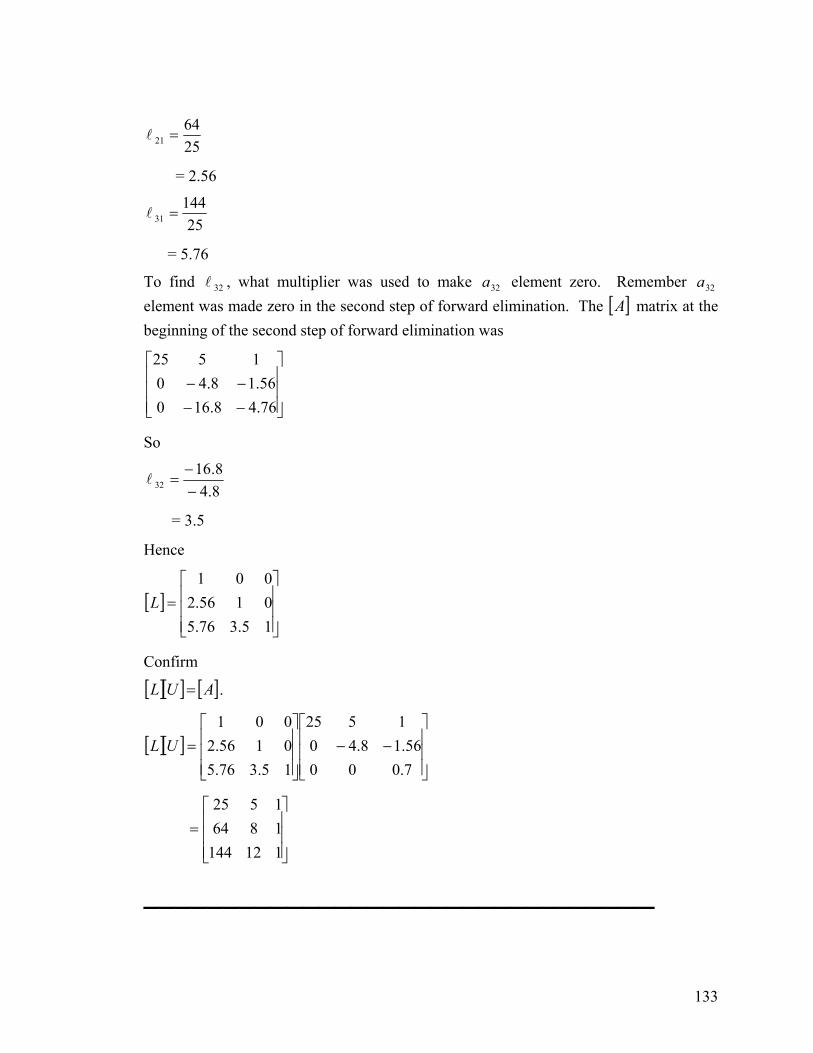
2564
21 =l
= 2.56
25144
31 =l
= 5.76
To find , what multiplier was used to make element zero. Remember element was made zero in the second step of forward elimination. The [ matrix at the beginning of the second step of forward elimination was
32l 32a 32a]A
⎥⎥⎥
⎦
⎤
⎢⎢⎢
⎣
⎡
−−−−
76.48.16056.18.40
1525
So
8.48.16
32 −−
=l
= 3.5
Hence
[ ]⎥⎥⎥
⎦
⎤
⎢⎢⎢
⎣
⎡=
15.376.50156.2001
L
Confirm
[ ][ ] [ ]AUL = .
[ ][ ]⎥⎥⎥
⎦
⎤
⎢⎢⎢
⎣
⎡−−
⎥⎥⎥
⎦
⎤
⎢⎢⎢
⎣
⎡=
7.00056.18.40
1525
15.376.50156.2001
UL
⎥⎥⎥
⎦
⎤
⎢⎢⎢
⎣
⎡=
11214418641525
________________________________
133

Example Use LU decomposition method to solve the following simultaneous linear equations.
⎥⎥⎥
⎦
⎤
⎢⎢⎢
⎣
⎡=
⎥⎥⎥
⎦
⎤
⎢⎢⎢
⎣
⎡
⎥⎥⎥
⎦
⎤
⎢⎢⎢
⎣
⎡
2.2792.1778.106
aaa
11214418641525
3
2
1
Solution Recall that
[ ][ ] [ ]CXA =
and if
[ ] [ ][ ]ULA =
then first solving
[ ][ ] [ ]CZL =
and then
[ ][ ] [ ]ZXU =
gives the solution vector [ ] . X
Now in the previous example, we showed
[ ] [ ][ ]⎥⎥⎥
⎦
⎤
⎢⎢⎢
⎣
⎡−−
⎥⎥⎥
⎦
⎤
⎢⎢⎢
⎣
⎡==
7.00056.18.40
1525
15.376.50156.2001
ULA
First solve
[ ][ ] [ ]CZL =
⎥⎥⎥
⎦
⎤
⎢⎢⎢
⎣
⎡=
⎥⎥⎥
⎦
⎤
⎢⎢⎢
⎣
⎡
⎥⎥⎥
⎦
⎤
⎢⎢⎢
⎣
⎡
2.2792.1778.106
15.376.50156.2001
3
2
1
zzz
to give
z1 = 106.8
2.56z1 +z2 = 177.2
5.76 z1 + 3.5 z2 + z3 = 279.2
134

Forward substitution starting from the first equation gives
z1 =106.8
z2 = 177.2 – 2.56 z1
= 177.2 – 2.56 (106.8)
= -96.21
z3 = 279.2 – 5.76 z1 – 3.5z2
= 279.2 – 5.76(106.8) – 3.5(-96.21)
= 0.735
Hence
[ ]⎥⎥⎥
⎦
⎤
⎢⎢⎢
⎣
⎡=
3
2
1
zzz
Z
⎥⎥⎥
⎦
⎤
⎢⎢⎢
⎣
⎡−=
735.021.968.106
This matrix is same as the right hand side obtained at the end of the forward elimination steps of Naïve Gauss elimination method. Is this a coincidence?
Now solve
[ ][ ] [ ]ZXU =
⎥⎥⎥
⎦
⎤
⎢⎢⎢
⎣
⎡=
⎥⎥⎥
⎦
⎤
⎢⎢⎢
⎣
⎡
⎥⎥⎥
⎦
⎤
⎢⎢⎢
⎣
⎡−−
0.73596.21-
106.8
7.00056.18.40
1525
3
2
1
aaa
8.106525 321 =++ aaa
21.9656.18.4 32 −=−− aa
735.07.0 3 =a
From the third equation
735.07.0 3 =a
0.70.735a 3 =
135

1.050 =
Substituting the value of a3 in the second equation,
21.9656.18.4 32 −=−− aa
8.456.121.96 3
2 −+−
=a
a
( )4.8-
1.0501.5696.21- +=
7019. =
Substituting the value of in the first equation, 32 and aa
8.106525 321 =++ aaa
2558.106
321
aaa
−−=
( )25
050.170.1958.106 −−=
2900.0 =
The solution vector is
⎥⎥⎥
⎦
⎤
⎢⎢⎢
⎣
⎡=
⎥⎥⎥
⎦
⎤
⎢⎢⎢
⎣
⎡
050.170.19
2900.0
3
2
1
aaa
_________________________________ How do I find the inverse of a square matrix using LU Decomposition?
A matrix [ is the inverse of ]B [ ]A if [ ][ ] [ ] [ ][ ]ABIBA == . How can we use LU decomposition to find inverse of the matrix? Assume the first column of [ (the inverse of [A] is
]B
[b b12 ………….b ] T 11 1n
then from the above definition of inverse and definition of matrix multiplication.
136
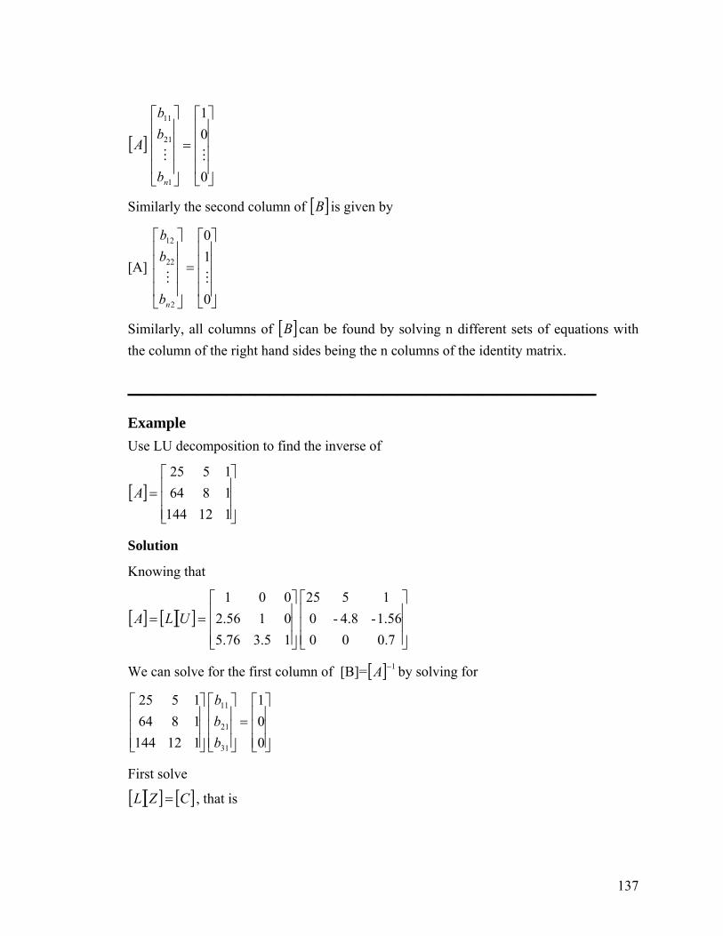
[ ]A
⎥⎥⎥⎥
⎦
⎤
⎢⎢⎢⎢
⎣
⎡
=
⎥⎥⎥⎥
⎦
⎤
⎢⎢⎢⎢
⎣
⎡
0
01
1
21
11
MM
nb
bb
Similarly the second column of [ ]B is given by
[A]
⎥⎥⎥⎥
⎦
⎤
⎢⎢⎢⎢
⎣
⎡
=
⎥⎥⎥⎥
⎦
⎤
⎢⎢⎢⎢
⎣
⎡
0
10
2
22
12
MM
nb
bb
Similarly, all columns of can be found by solving n different sets of equations with the column of the right hand sides being the n columns of the identity matrix.
[ ]B
_________________________________ Example Use LU decomposition to find the inverse of
[ ]⎥⎥⎥
⎦
⎤
⎢⎢⎢
⎣
⎡=
11214418641525
A
Solution
Knowing that
[ ] [ ][ ]⎥⎥⎥
⎦
⎤
⎢⎢⎢
⎣
⎡
⎥⎥⎥
⎦
⎤
⎢⎢⎢
⎣
⎡==
0.7001.56-4.8-01525
15.376.50156.2001
ULA
We can solve for the first column of [B]= [ ] 1−A by solving for
⎥⎥⎥
⎦
⎤
⎢⎢⎢
⎣
⎡=
⎥⎥⎥
⎦
⎤
⎢⎢⎢
⎣
⎡
⎥⎥⎥
⎦
⎤
⎢⎢⎢
⎣
⎡
001
11214418641525
31
21
11
bbb
First solve
[ ][ ] [ ]CZL = , that is
137

⎥⎥⎥
⎦
⎤
⎢⎢⎢
⎣
⎡=
⎥⎥⎥
⎦
⎤
⎢⎢⎢
⎣
⎡
⎥⎥⎥
⎦
⎤
⎢⎢⎢
⎣
⎡
001
15.376.50156.2001
3
2
1
zzz
to give
11 =z
056.2 21 =+ zz
05.376.5 321 =++ zzz
Forward substitution starting from the first equation gives
1 z1 =
12 2.56z-0 z =
( )156.20 −=
56.2−=
213 5.376.50 zzz −−=
( ) ( )56.25.3176.50 −−−=
2.3=
Hence
[ ]⎥⎥⎥
⎦
⎤
⎢⎢⎢
⎣
⎡=
3
2
1
zzz
Z
⎥⎥⎥
⎦
⎤
⎢⎢⎢
⎣
⎡−=
2.356.2
1
Now solve
[ ][ ] [ ]ZXU =
that is
138

⎥⎥⎥
⎦
⎤
⎢⎢⎢
⎣
⎡=
⎥⎥⎥
⎦
⎤
⎢⎢⎢
⎣
⎡
⎥⎥⎥
⎦
⎤
⎢⎢⎢
⎣
⎡−−
3.22.56-1
7.00056.18.40
1525
31
21
11
bbb
1525 312111 =++ bbb
56.256.18.4 3121 −=−− bb
2.37.0 31 =b
Backward substitution starting from the third equation gives
7.02.3
31 =b
= 571.4
8.4560.156.2 31
21 −+−
=b
b
8.4
)571.4(560.156.2−
+−=
= -0.9524
2551 3121
11bb
b−−
=
25
571.4)9524.0(51 −−−=
= 0.04762
Hence the first column of the inverse of [A] is
⎥⎥⎥
⎦
⎤
⎢⎢⎢
⎣
⎡−=
⎥⎥⎥
⎦
⎤
⎢⎢⎢
⎣
⎡
571.49524.0
04762.0
31
21
11
bbb
Similarly by solving
⎥⎥⎥
⎦
⎤
⎢⎢⎢
⎣
⎡=
⎥⎥⎥
⎦
⎤
⎢⎢⎢
⎣
⎡
⎥⎥⎥
⎦
⎤
⎢⎢⎢
⎣
⎡
010
11214418641525
32
22
12
bbb
139

⎥⎥⎥
⎦
⎤
⎢⎢⎢
⎣
⎡
−
−=
⎥⎥⎥
⎦
⎤
⎢⎢⎢
⎣
⎡
000.5417.108333.0
32
22
12
bbb
and solving
⎥⎥⎥
⎦
⎤
⎢⎢⎢
⎣
⎡=
⎥⎥⎥
⎦
⎤
⎢⎢⎢
⎣
⎡
⎥⎥⎥
⎦
⎤
⎢⎢⎢
⎣
⎡
100
bbb
11214418641525
33
23
13
gives
⎥⎥⎥
⎦
⎤
⎢⎢⎢
⎣
⎡−=
⎥⎥⎥
⎦
⎤
⎢⎢⎢
⎣
⎡
429.14643.0
03571.0
33
23
13
bbb
Hence
[ ]⎥⎥⎥
⎦
⎤
⎢⎢⎢
⎣
⎡
−−−=−
429.1050.5571.44643.0417.19524.0
0357.008333.04762.01A
Can you confirm the following for the above example? [ ][ ] [ ]IAA =−1 [ ]AA 1−= [ ]
_________________________________ Key Terms LU decomposition Inverse
_________________________________ Homework
1.
Show that LU decomposition is computationally more efficient way of finding the inverse of a square matrix than using Gaussian elimination.
2.
LU decomposition method is computationally
140

more efficient than Naïve Gauss elimination for
A. Solving a single set of simultaneous linear equations
B. Solving multiple sets of simultaneous linear equations with different coefficient matrices.
C. Solving multiple sets of simultaneous linear equations with same coefficient matrix but different right hand sides.
D. Solving less than ten simultaneous linear equations.
3.
It one decomposes a symmetric matrix [A] to a LU form, then
A. [L] = [U]T
B. [U]T = [L]T
A. [L] = [U]
D. [L] = [I]
4.
Use LU decomposition to solve
6642524
321
321
321
=++=++−=−+
xxxxxx
xxx
Answer: (3, -13, 1)
5.
Find the inverse of
141
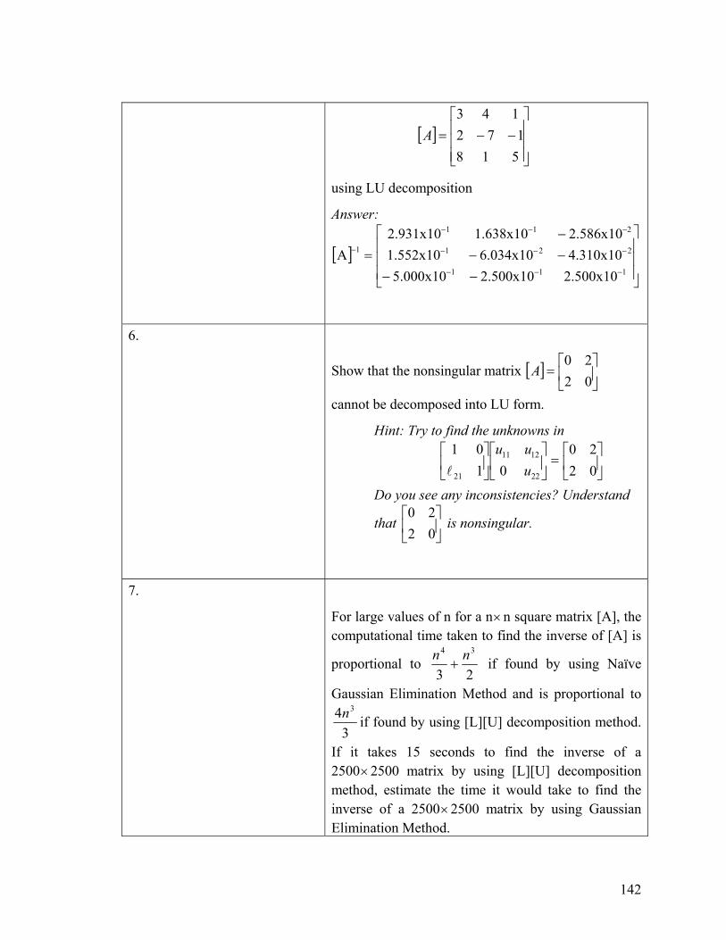
[ ]⎥⎥⎥
⎦
⎤
⎢⎢⎢
⎣
⎡−−=518172
143A
using LU decomposition
Answer:
[ ]⎥⎥⎥
⎦
⎤
⎢⎢⎢
⎣
⎡
−−−−−
=−−−
−−−
−−−
−
111
221
211
1
2.500x102.500x105.000x104.310x106.034x101.552x102.586x101.638x102.931x10
A
6.
Show that the nonsingular matrix
cannot be decomposed into LU form.
[ ] ⎥⎦
⎤⎢⎣
⎡=
0220
A
Hint: Try to find the unknowns in
⎥⎦
⎤⎢⎣
⎡=⎥
⎦
⎤⎢⎣
⎡⎥⎦
⎤⎢⎣
⎡0220
0101
22
1211
21 uuu
l
Do you see any inconsistencies? Understand
that is nonsingular. ⎥⎦
⎤⎢⎣
⎡0220
7.
For large values of n for a n×n square matrix [A], the computational time taken to find the inverse of [A] is
proportional to 23
34 nn+ if found by using Naïve
Gaussian Elimination Method and is proportional to
34 3n if found by using [L][U] decomposition method.
If it takes 15 seconds to find the inverse of a 2500×2500 matrix by using [L][U] decomposition method, estimate the time it would take to find the inverse of a 2500×2500 matrix by using Gaussian Elimination Method.
142

143
Chapter 8 Gauss-Siedel Method _________________________ After reading this chapter, you will be able to
Solve a set of equations using Gauss-Siedel method
Learn the advantages and pitfalls of Gauss-Siedel method
Understand under what conditions Gauss-Siedel method always converges
_________________________________
Why do we need another method to solve a set of simultaneous linear equations?
In certain cases, such as when a system of equations is large, iterative methods of solving equations such as Gauss-Siedel method are more advantageous. Elimination methods such as Gaussan elimination, are prone to round off errors for a large set of equations. Iterative methods, such as Guass-Siedel method, allow the user the control of the round-off error. Also if the physics of the problem are well known for faster convergence, initial guesses needed in iterative methods can be made more judiciously. You convinced me, so what is the algorithm for Gauss-Siedel method? Given a general set of n equations and n unknowns, we have
11313212111 ... cxaxaxaxa nn =++++
22323222121 ... cxaxaxaxa nn =++++
. .
. .
. .
nnnnnnn cxaxaxaxa =++++ ...332211
If the diagonal elements are non-zero, each equation is rewritten for the corresponding unknown, that is, the first equation is rewritten with on the left hand side, second equation is rewritten with on the left hand side and so on as follows
1x
2x
144
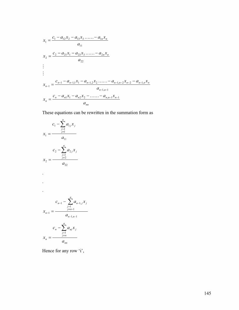
11
131321211 a
xaxaxacx nn−−−=
KK
nn
nnnnnnn
nn
nnnnnnnnnn
nn
axaxaxac
x
axaxaxaxac
x
axaxaxac
x
11,2211
1,1
,122,122,111,111
22
232312122
−−
−−
−−−−−−−−
−−−−=
−−−−=
−−−=
KK
KK
M
M
KK
These equations can be rewritten in the summation form as
11
11
11
1 a
xac
x
n
jj
jj∑≠=
−
=
22
21
22
2 a
xac
x
j
n
jj
j∑≠=
−
=
.
.
.
1,1
11
,11
1−−
−≠=
−−
−
∑−
=nn
n
njj
jjnn
n a
xac
x
nn
n
njj
jnjn
n a
xac
x
∑≠=
−
=1
Hence for any row ‘i’,
145

.,,2,1,1
nia
xac
xii
n
ijj
jiji
i K=
−
=
∑≠=
Now to find xi’s, one assumes an initial guess for the xi’s and then use the rewritten equations to calculate the new guesses. Remember, one always uses the most recent guesses to calculate xi. At the end of each iteration, one calculates the absolute relative approximate error for each xi as
100xx
xxnewi
oldi
newi
ia
−=ε
where is the recently obtained value of xnewix i, and is the previous value of xold
ix i.
When the absolute relative approximate error for each xi is less than the prespecified tolerance, the iterations are stopped.
___________________________ Example
The upward velocity of a rocket is given at three different times in the following table
Time, t Velocity, v
S m/s
5 106.8
8 177.2
12 279.2
The velocity data is approximated by a polynomial as
( ) 12.t5 , 322
1 ≤≤++= atatatv
The coefficients a1, a2, a3 for the above expression were found in Chapter 5 to be given by
⎥⎥⎥
⎦
⎤
⎢⎢⎢
⎣
⎡=
⎥⎥⎥
⎦
⎤
⎢⎢⎢
⎣
⎡
⎥⎥⎥
⎦
⎤
⎢⎢⎢
⎣
⎡
2.2792.1778.106
aaa
11214418641525
3
2
1
146
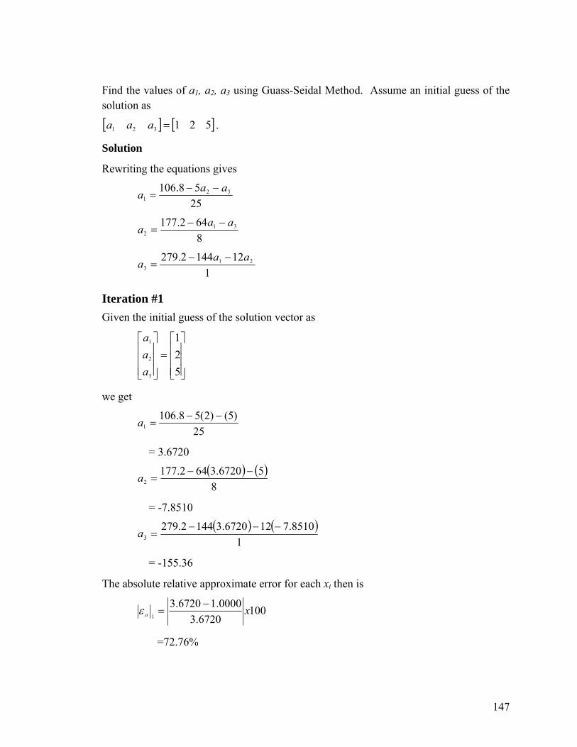
Find the values of a1, a2, a3 using Guass-Seidal Method. Assume an initial guess of the solution as
[ ] [ 521321 =aaa ] . Solution
Rewriting the equations gives
2558.106 32
1
aaa −−=
8642.177 31
2
aaa −−=
1
121442.279 213
aaa −−=
Iteration #1 Given the initial guess of the solution vector as
⎥⎥⎥
⎦
⎤
⎢⎢⎢
⎣
⎡=
⎥⎥⎥
⎦
⎤
⎢⎢⎢
⎣
⎡
521
3
2
1
aaa
we get
25
)5()2(58.1061
−−=a
= 3.6720
( ) ( )8
56720.3642.1772
−−=a
= -7.8510
( ) ( )1
8510.7126720.31442.2793
−−−=a
= -155.36
The absolute relative approximate error for each xi then is
1006720.3
0000.16720.31
xa
−=ε
=72.76%
147

1008510.7
0000.28510.72
xa −−−
=ε
=125.47%
10036.155
0000.536.1553
xa −−−
=ε
= 103.22%
At the end of the first iteration, the guess of the solution vector is
⎥⎥⎥
⎦
⎤
⎢⎢⎢
⎣
⎡
−−=
⎥⎥⎥
⎦
⎤
⎢⎢⎢
⎣
⎡
36.1558510.7
6720.3
3
2
1
aaa
and the maximum absolute relative approximate error is 125.47%.
Iteration #2 The estimate of the solution vector at the end of iteration #1 is
⎥⎥⎥
⎦
⎤
⎢⎢⎢
⎣
⎡
−−=
⎥⎥⎥
⎦
⎤
⎢⎢⎢
⎣
⎡
36.1558510.7
6720.3
3
2
1
aaa
Now we get
( )25
36.1558510.758.1061
−−−=a
= 12.056
( )8
36.155056.12642.1772
−−=a
= -54.882
( ) ( )1
882.5412056.121442.2793
−−−=a
=-798.34
The absolute relative approximate error for each then is ix
100056.12
6720.3056.121
xa−
=∈
= 69.542%
148
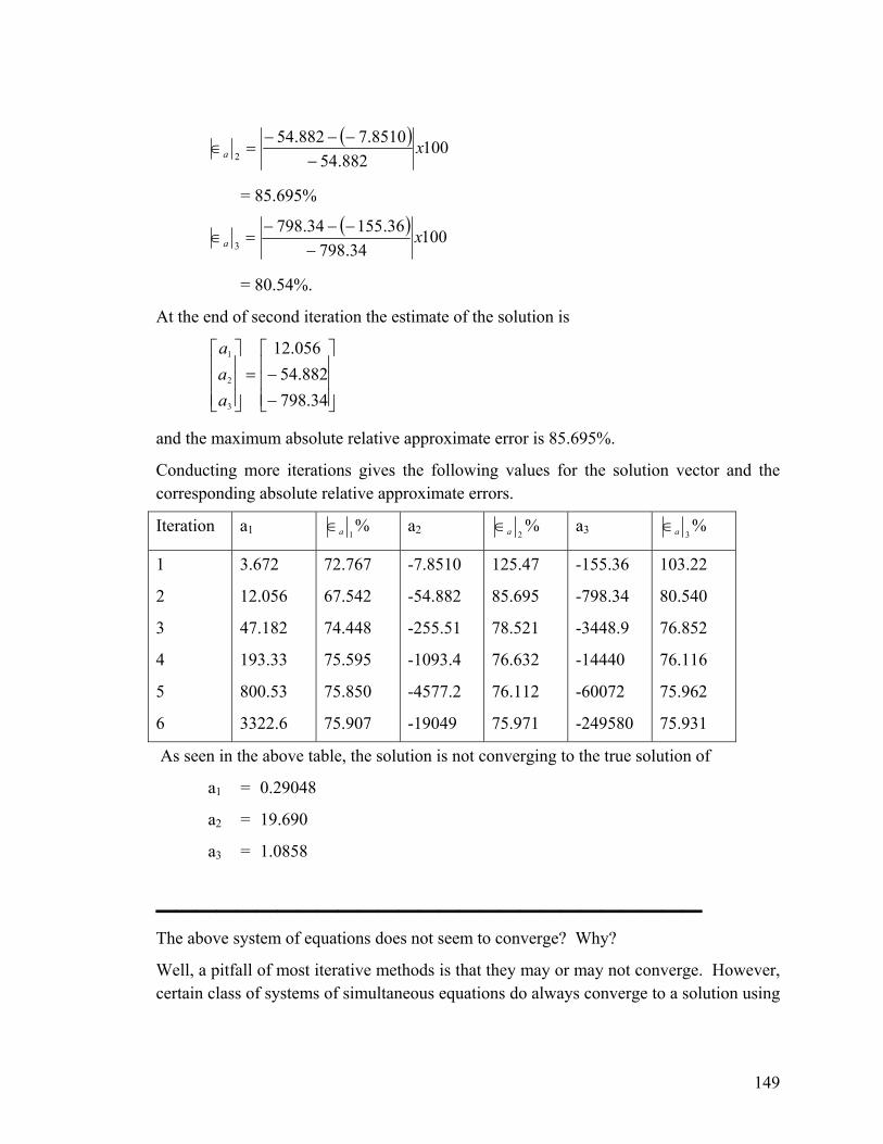
( ) 100882.54
8510.7882.542
xa −−−−
=∈
= 85.695%
( ) 10034.798
36.15534.7983
xa −−−−
=∈
= 80.54%.
At the end of second iteration the estimate of the solution is
⎥⎥⎥
⎦
⎤
⎢⎢⎢
⎣
⎡
−−=
⎥⎥⎥
⎦
⎤
⎢⎢⎢
⎣
⎡
34.798882.54
056.12
3
2
1
aaa
and the maximum absolute relative approximate error is 85.695%.
Conducting more iterations gives the following values for the solution vector and the corresponding absolute relative approximate errors.
Iteration a1 %1a∈ a2 %
2a∈ a3 %3a∈
1
2
3
4
5
6
3.672
12.056
47.182
193.33
800.53
3322.6
72.767
67.542
74.448
75.595
75.850
75.907
-7.8510
-54.882
-255.51
-1093.4
-4577.2
-19049
125.47
85.695
78.521
76.632
76.112
75.971
-155.36
-798.34
-3448.9
-14440
-60072
-249580
103.22
80.540
76.852
76.116
75.962
75.931
As seen in the above table, the solution is not converging to the true solution of
a1 = 0.29048
a2 = 19.690
a3 = 1.0858
___________________________ The above system of equations does not seem to converge? Why?
Well, a pitfall of most iterative methods is that they may or may not converge. However, certain class of systems of simultaneous equations do always converge to a solution using
149
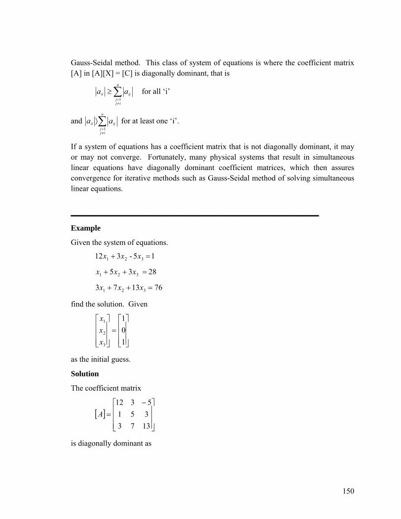
Gauss-Seidal method. This class of system of equations is where the coefficient matrix [A] in [A][X] = [C] is diagonally dominant, that is
∑≠=
≥n
ijj
ijii aa1
for all ‘i’
and ∑≠=
⟩n
ijj
ijii aa1
for at least one ‘i’.
If a system of equations has a coefficient matrix that is not diagonally dominant, it may or may not converge. Fortunately, many physical systems that result in simultaneous linear equations have diagonally dominant coefficient matrices, which then assures convergence for iterative methods such as Gauss-Seidal method of solving simultaneous linear equations.
___________________________ Example
Given the system of equations.
1 5 -3 12 321 =+ xxx
28 3 5 321 =++ xxx
76 13 7 3 321 =++ xxx
find the solution. Given
⎥⎥⎥
⎦
⎤
⎢⎢⎢
⎣
⎡=
⎥⎥⎥
⎦
⎤
⎢⎢⎢
⎣
⎡
101
3
2
1
xxx
as the initial guess.
Solution
The coefficient matrix
[ ]⎥⎥⎥
⎦
⎤
⎢⎢⎢
⎣
⎡ −=
13733515312
A
is diagonally dominant as
150

8531212 131211 =−+=+≥== aaa
43155 232122 =+=+≥== aaa
10731313 323133 =+=+≥== aaa
and the inequality is strictly greater than for at least one row. Hence the solution should converge using Gauss-Seidal method.
Rewriting the equations, we get
12
531 321
xxx +−=
5
328 312
xxx −−=
13
7376 213
xxx −−=
Assuming an initial guess of
⎥⎥⎥
⎦
⎤
⎢⎢⎢
⎣
⎡=
⎥⎥⎥
⎦
⎤
⎢⎢⎢
⎣
⎡
101
3
2
1
xxx
Iteration 1:
( ) ( )12
150311
+−=x
= 0.50000
( ) ( )5
135.0282
−−=x
= 4.9000
( ) ( )13
9000.4750000.03763
−−=x
= 3.0923
The absolute relative approximate error at the end of first iteration is
10050000.0
0000.150000.01
xa−
=∈
151
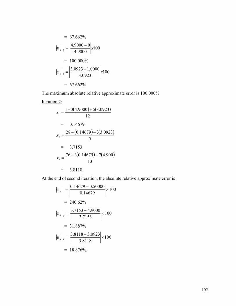
= 67.662%
1009000.4
09000.42
xa−
=∈
= 100.000%
1000923.3
0000.10923.33
xa−
=∈
= 67.662%
The maximum absolute relative approximate error is 100.000%
Iteration 2:
( ) ( )12
0923.359000.4311
+−=x
= 0.14679
( ) ( )5
0923.3314679.0282
−−=x
= 3.7153
( ) ( )13
900.4714679.03763
−−=x
= 3.8118
At the end of second iteration, the absolute relative approximate error is
10014679.0
50000.014679.01
×−
=∈a
= 240.62%
1007153.3
9000.47153.32
×−
=∈a
= 31.887%
1008118.3
0923.38118.33
×−
=∈a
= 18.876%.
152

The maximum absolute relative approximate error is 240.62%. This is greater than the value of 67.612% we obtained in the first iteration. Is the solution diverging? No, as you conduct more iterations, the solution converges as follows.
Iteration a1 1aε a2 2aε a3 3aε
1
2
3
4
5
6
0.50000
0.14679
0.74275
0.94675
0.99177
0.99919
67.662
240.62
80.23
21.547
4.5394
0.74260
4.900
3.7153
3.1644
3.0281
3.0034
3.0001
100.00
31.887
17.409
4.5012
0.82240
0.11000
3.0923
3.8118
3.9708
3.9971
4.0001
4.0001
67.662
18.876
4.0042
0.65798
0.07499
0.00000
This is close to the exact solution vector of
⎥⎥⎥
⎦
⎤
⎢⎢⎢
⎣
⎡=
⎥⎥⎥
⎦
⎤
⎢⎢⎢
⎣
⎡
431
3
2
1
xxx
___________________________ Example
Given the system of equations
76 13x 7x 3x 321 =++
28 3x 5x x 321 =++
1 5x - 3x 12x 32 1 =+
find the solution using Gauss-Seidal method. Use [ ] [ ]101,, 321 =xxx as the initial guess.
Solution
Rewriting the equations, we get
3
13776 321
xxx −−=
5
328 312
xxx −−=
153

5
3121 213 −
−−=
xxx
Assuming an initial guess of
⎥⎥⎥
⎦
⎤
⎢⎢⎢
⎣
⎡=
⎥⎥⎥
⎦
⎤
⎢⎢⎢
⎣
⎡
101
3
2
1
xxx
the next six iterative values are given in the table below
Iteration a1 1a∈ a2 2a∈ a3 3a∈
1
2
3
4
5
6
21.000
-196.15
-1995.0
-20149
2.0364x10⁵
-2.0579x10⁵
110.71
109.83
109.90
109.89
109.90
1.0990
0.80000
14.421
-116.02
1204.6
-12140
1.2272x10⁵
100.00
94.453
112.43
109.63
109.92
109.89
5.0680
-462.30
4718.1
-47636
4.8144x10⁵
-4.8653x10⁶
98.027
110.96
109.80
109.90
109.89
109.89
You can see that this solution is not converging and the coefficient matrix is not diagonally dominant. The coefficient matrix
[ ]⎥⎥⎥
⎦
⎤
⎢⎢⎢
⎣
⎡
−=
5312351
1373A
is not diagonally dominant as
2013733 131211 =+=+≤== aaa
Hence Gauss-Seidal method may or may not converge.
However, it is the same set of equations as the previous example and that converged. The only difference is that we exchanged first and the third equation with each other and that made the coefficient matrix not diagonally dominant.
So it is possible that a system of equations can be made diagonally dominant if one exchanges the equations with each other. But it is not possible for all cases. For example, the following set of equations.
3321 =++ xxx
154

9
9
432 321 =++ xxx
7 321 =++ xxx
can not be rewritten to make the coefficient matrix diagonally dominant.
___________________________ Homework
1. In a system of equation [A] [X] = [C], if [A] is diagonally dominant, then Gauss-Seidal method
A. always converges
B. may or may not converge
C. always diverges
2.
In a system of equations [A] [X] = [C], if [A] is not diagonally dominant, then Gauss-Seidal method
D. Always converges
E. May or may not converge
F. Always diverges.
3.
In a system of equations [A] [X] = [C], if [A] is not diagonally dominant, the system of equations can always be rewritten to make it diagonally dominant.
G. True
H. False
155

4.
Solve the following system of equations using Gauss-Seidal method
23712 321 x x x =++
5
6
5 321 - x x x =++
1172 321 =−+ xxx
Conduct 3 iterations, calculate the maximum absolute relative approximate error at the end of each iteration and choose [ ] [ ]531321 =xxx as your initial guess.
Answer: [ ] [ ]0243.10115.190666.0321 −−=xxx
[ ] [ ]%099.17%564.10%001.65321=∈∈∈ aaa
[ ] [ ]%099.17%564.10%001.65321=∈∈∈ aaa
156
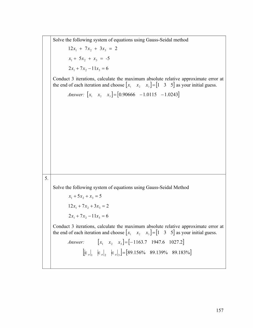
Solve the following system of equations using Gauss-Seidal method
3712 321 x x x =++ 2
55 321 - x x x =++
61172 321 =−+ xxx
Conduct 3 iterations, calculate the maximum absolute relative approximate error at the end of each iteration and choose [ ] [ ]531321 =xxx as your initial guess.
[ ] [ ]0243.10115.190666.0321 −−=xxx Answer:
5.
Solve the following system of equations using Gauss-Seidal Method
5 321 =++ xxx 5
2 3712 321 =++ xxx
1172 321 =−+ xxx 6
Conduct 3 iterations, calculate the maximum absolute relative approximate error at the end of each iteration and choose [ ] [ ]531321 =xxx as your initial guess.
[ ] [ ]2.10276.19477.1163321 −=xxxAnswer:
[ ] [ ]%183.89%139.89%156.89321=∈∈∈ aaa
157

Chapter 9 Adequacy of Solutions _________________________ After reading this chapter, you will be able to
Know the difference between ill conditioned and well conditioned system of equations
Define the norm of a matrix
Relate the norm of the matrix and of its inverse to the ill or well conditioning of the matrix, that is, how much trust can you have in the solution of the matrix.
_________________________________
What does it mean by ill conditioned and well-conditioned system of equations?
A system of equations is considered to be well conditioned if a small change in the coefficient matrix or a small change in the right hand side results in a small change in the solution vector.
A system of equations is considered to be ill conditioned if a small change in the coefficient matrix or a small change in the right hand side results in a large change in the solution vector.
_________________________________
Example
Is this system of equations well conditioned?
⎥⎦
⎤⎢⎣
⎡=⎥
⎦
⎤⎢⎣
⎡⎥⎦
⎤⎢⎣
⎡999.74
999.3221
yx
Solution
The solution to the above set of equations is
⎥⎦
⎤⎢⎣
⎡=⎥
⎦
⎤⎢⎣
⎡12
yx
158

Make a small change in the right hand side vector of the equations
⎥⎦
⎤⎢⎣
⎡−=⎥
⎦
⎤⎢⎣
⎡
⎥⎦
⎤⎢⎣
⎡=⎥
⎦
⎤⎢⎣
⎡⎥⎦
⎤⎢⎣
⎡
000.4999.3
998.7001.4
999.3221
yx
givesyx
Make a small change in the coefficient matrix of the equations
⎥⎦
⎤⎢⎣
⎡=⎥
⎦
⎤⎢⎣
⎡
⎥⎦
⎤⎢⎣
⎡=⎥
⎦
⎤⎢⎣
⎡⎥⎦
⎤⎢⎣
⎡
001388.0994.3
999.74
998.3001.2001.2001.1
yx
givesyx
This system of equation “looks” ill conditioned as a small change in the coefficient matrix or the right hand side resulted in a large change in the solution vector.
_________________________________
Example
Is this system of equations well conditioned?
⎥⎦
⎤⎢⎣
⎡=⎥
⎦
⎤⎢⎣
⎡⎥⎦
⎤⎢⎣
⎡74
3221
yx
Solution
The solution to the above equations is
⎥⎦
⎤⎢⎣
⎡=⎥
⎦
⎤⎢⎣
⎡12
yx
Make a small change in the right hand side vector of the equations.
⎥⎦
⎤⎢⎣
⎡=⎥
⎦
⎤⎢⎣
⎡⎥⎦
⎤⎢⎣
⎡001.7001.4
3221
yx
gives
159
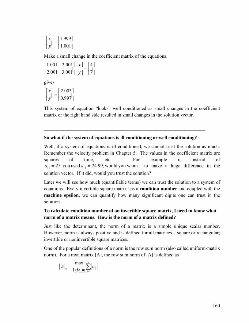
⎥⎦
⎤⎢⎣
⎡=⎥
⎦
⎤⎢⎣
⎡001.1999.1
yx
Make a small change in the coefficient matrix of the equations.
⎥⎦
⎤⎢⎣
⎡=⎥
⎦
⎤⎢⎣
⎡⎥⎦
⎤⎢⎣
⎡74
001.3001.2001.2001.1
yx
gives
⎥⎦
⎤⎢⎣
⎡=⎥
⎦
⎤⎢⎣
⎡997.0003.2
yx
This system of equation “looks” well conditioned as small changes in the coefficient matrix or the right hand side resulted in small changes in the solution vector.
_________________________________
So what if the system of equations is ill conditioning or well conditioning?
Well, if a system of equations is ill conditioned, we cannot trust the solution as much. Remember the velocity problem in Chapter 5. The values in the coefficient matrix are squares of time, etc. For example if instead of
to make a huge difference in the solution vector. If it did, would you trust the solution?
ityou want would,99.24 usedyou ,25 1111 == aa
Later we will see how much (quantifiable terms) we can trust the solution to a system of equations. Every invertible square matrix has a condition number and coupled with the machine epsilon, we can quantify how many significant digits one can trust in the solution.
To calculate condition number of an invertible square matrix, I need to know what norm of a matrix means. How is the norm of a matrix defined?
Just like the determinant, the norm of a matrix is a simple unique scalar number. However, norm is always positive and is defined for all matrices – square or rectangular; invertible or noninvertible square matrices.
One of the popular definitions of a norm is the row sum norm (also called uniform-matrix norm). For a mxn matrix [A], the row sum norm of [A] is defined as
∑=
∞ <<=
n
jija
miA
11max
160

that is, find the sum of the absolute of the elements of each row of the matrix [A]. The maximum out of the ‘m’ such values is the row sum norm of the matrix [A].
_________________________________
Example
Find the row sum norm of the following matrix [A].
⎥⎥⎥
⎦
⎤
⎢⎢⎢
⎣
⎡
−−
−=
5156099.230710
A
Solution
( ) ( ) ( )[ ]515,6099.23,0710max
31max 3
1
+−+++−+−+
<<= ∑
=∞
jija
iA
( ) ( ) ( )[ ]515,6099.23,0710max ++++++=
[ ]11,099.11,17max=
.17=
_________________________________
How is norm related to the conditioning of the matrix?
Let us start answering this question using an example. Go back to the “ill conditioned” system of equations,
⎥⎦
⎤⎢⎣
⎡=⎥
⎦
⎤⎢⎣
⎡⎥⎦
⎤⎢⎣
⎡999.74
yx
999.3221
that gives the solution as
⎥⎦
⎤⎢⎣
⎡=⎥
⎦
⎤⎢⎣
⎡12
yx
Denoting the above set of equations as
[ ][ ] [ ]CXA =
2X =∞
161
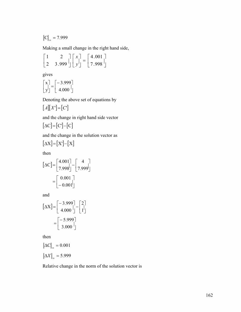
999.7C =∞
Making a small change in the right hand side,
⎥⎦
⎤⎢⎣
⎡=⎥
⎦
⎤⎢⎣
⎡⎥⎦
⎤⎢⎣
⎡998.7001.4
999.3221
yx
gives
⎥⎦
⎤⎢⎣
⎡−=⎥
⎦
⎤⎢⎣
⎡000.4999.3
yx
Denoting the above set of equations by
[ ][ ] [ ]'' CXA =
and the change in right hand side vector
[ ] [ ] [C'CC −=Δ ]
]
and the change in the solution vector as
[ ] [ ] [X'XX −=Δ
then
[ ] ⎥⎦
⎤⎢⎣
⎡−⎥
⎦
⎤⎢⎣
⎡=Δ
999.74
998.7001.4
C
⎥⎦
⎤⎢⎣
⎡−
=001.0
001.0
and
[ ] ⎥⎦
⎤⎢⎣
⎡−⎥
⎦
⎤⎢⎣
⎡−=Δ
12
000.4999.3
X
⎥⎦
⎤⎢⎣
⎡−=
000.3999.5
then
001.0C =Δ∞
999.5=Δ∞
X
Relative change in the norm of the solution vector is
162

9995.2
2999.5
=
=Δ
∞
∞
XX
Relative change in the norm of the right hand side vector is
410250.1
999.7001.0
−
∞
∞
×=
=Δ
CC
See the small relative change in the right hand side vector of 1.250 ×10⁻⁴ results in a large relative change in the solution vector as 2.995.
In fact, the ratio between the relative change in the norm of the solution vector to the relative change in the norm of the right hand side vector is
2395710250.1
9995.2
//
4
=×
=
Δ
Δ
−
∞∞
∞∞
CCXX
Let us now go back to the “well-conditioned” system of equations.
⎥⎦
⎤⎢⎣
⎡=⎥
⎦
⎤⎢⎣
⎡⎥⎦
⎤⎢⎣
⎡74
yx
3221
gives
⎥⎦
⎤⎢⎣
⎡=⎥
⎦
⎤⎢⎣
⎡12
yx
Denoting the system of equations as
[ ][ ] [ ]CXA =
2X =∞
7C =∞
Making a small change in the right hand side vector
⎥⎦
⎤⎢⎣
⎡=⎥
⎦
⎤⎢⎣
⎡⎥⎦
⎤⎢⎣
⎡001.7001.4
yx
3221
gives
163

⎥⎦
⎤⎢⎣
⎡=⎥
⎦
⎤⎢⎣
⎡001.1999.1
yx
Denoting the above set of equations as
[ ][ ] [ ]'C'XA =
and the change in the right hand side vector
[ ] [ ] [CCC −=Δ ' ]
]
and the change in the solution vector as
[ ] [ ] [XXX −=Δ '
then
[ ] ⎥⎦
⎤⎢⎣
⎡−⎥
⎦
⎤⎢⎣
⎡=Δ
74
001.7001.4
C ⎥⎦
⎤⎢⎣
⎡=
001.0001.0
and
[ ] ⎥⎦
⎤⎢⎣
⎡−⎥
⎦
⎤⎢⎣
⎡=Δ
12
001.1999.1
X ⎥⎦
⎤⎢⎣
⎡−=
001.0001.0
then
001.0C =Δ∞
001.0X =Δ∞
Relative change in the norm of solution vector is
2001.0
=
Δ
∞
∞
XX
4105 −×=
Relative change in the norm of the right hand side vector is
7001.0
=
Δ
∞
∞
CC
= 410429.1 −×
164

See a small relative change in the right hand side vector norm of 1.429 ×10⁻⁴ results in a small relative change in the solution vector norm of 5 10-4. ×
In fact, the ratio between the relative change in the norm of the solution vector to the relative change in the norm of the right hand side vector is
4104291
4105
//
−×
−×=
Δ
Δ
∞∞
∞∞
.
CCXX
=3.5
What are some of the properties of norms?
0≥A1. For a matrix [A],
AkkA =2. For a matrix [A] and a scalar k,
3. For two matrices [A] and [B] of same order,
BABA +≤+
4. For two matrices [A] and [B] that can be multiplied as [A] [B],
BAAB ≤
Is there a general relationship that exists between or between C/CandX/X ΔΔ
and X/XΔ A/AΔ ? If so, it could help us identify well-conditioned and ill
conditioned system of equations.
If there is such a relationship, will it help us quantify the conditioning of the matrix, that is, tell us how many significant digits we could trust in the solution of a system of simultaneous linear equations?
There is a relationship that exists between
CC
andXX ΔΔ
, and between
AA
andXX ΔΔ
.
These relationships are
165
CC
AAXX
X Δ≤
Δ+
Δ −1 .
AA
AAXX 1 Δ
<Δ −
Looking at the above two inequalities, it shows that the relative change in the norm of the right hand side vector or the coefficient matrix 1AA −can be amplified by as much as .
1AA −This number is called the condition number of the matrix and coupled with
the machine epsilon, we can quantify the accuracy of the solution of [A][X] = [C].
Prove for [ ] [ ] [ ]CXA =
AA
AAXX
X 1 Δ⟨
Δ+
Δ − .
Proof
Let
[ ] [ ] [ ]CXA = (1)
Then if [A] is changed to , then[X] will change to [ 'A ] [ ]'X , such
that
[ ] [ ] [ ]C'X'A = (2)
From equations (1) and (2),
[ ] [ ] [ ][ ]' ' XAXA =
Denoting change in [A] and [X] matrices as
[ ] [ ] [A'AA −=Δ ]]
[ ] [ ] [X'XX −=Δ
then
[ ][ ] [ ] [ ]( ) [ ] [ ]( )XXAAXA Δ+Δ+=
Expanding the above expression
[ ][ ] [ ][ ] [ ][ ] [ ][ ] [ ][ ]XAXAXAXAXA ΔΔ+Δ+Δ+=
166

[ ][ ] [ ] [ ] [ ]( )XXAXA Δ+Δ+Δ= 0
[ ][ ] [ ] [ ] [ ]( )XXAXA Δ+Δ=Δ−
[ ] [ ] [ ] [ ] [ ]( )XXAAX 1 Δ+Δ−=Δ −
Applying the theorem of norms that norm of multiplied matrices is less than the multiplication of the individual norms of the matrices,
XXAAX 1 Δ+Δ<Δ −
A Multiplying both sides by
XXAAAXA 1 Δ+Δ<Δ −
AA
AAXX
X 1 Δ<
Δ+
Δ −
How do I use the above theorems to find how many significant digits are correct in my solution vector?
Relative error in solution vector is <= Cond (A)* relative error in right hand side.
Possible relative error in the solution vector is <= Cond (A) * mach∈
Hence Cond (A)* should give us the number of significant digits at least correct in our solution by comparing it with 0.5
mach∈
×10-m.
_________________________________
Example
How many significant digits can I trust in the solution of the following system of equations?
⎥⎦
⎤⎢⎣
⎡=⎥
⎦
⎤⎢⎣
⎡⎥⎦
⎤⎢⎣
⎡42
yx
999.3221
Solution
[ ] ⎥⎦
⎤⎢⎣
⎡=
999.3221
A
[ ] ⎥⎦
⎤⎢⎣
⎡−
−=−
1.10001.20001.200031.3999
A 1
167

999.5A =∞
4.5999A 1 =∞
−
( )∞
−∞
= 1AAACond
4.5999999.5 ×=
35990=
Assuming single precision with 24 bits used in the mantissa for real numbers, the machine epsilon
6
241
10119209.0
2−
−
×=
=∈mach
2
6
104290.010119209.035990
)*(
−
−
=
××=
∈
x
ACond mach
Comparing it with m105.0 −×2m 104290.0105.0 −− ×<×
2m<
So two significant digits are at least correct in the solution vector.
_________________________________
Example
How many significant digits can I trust in the solution of the following system of equations?
⎥⎦
⎤⎢⎣
⎡=⎥
⎦
⎤⎢⎣
⎡⎥⎦
⎤⎢⎣
⎡74
yx
3221
Solution
For
[ ] ⎥⎦
⎤⎢⎣
⎡=
3221
A
it can be shown
168
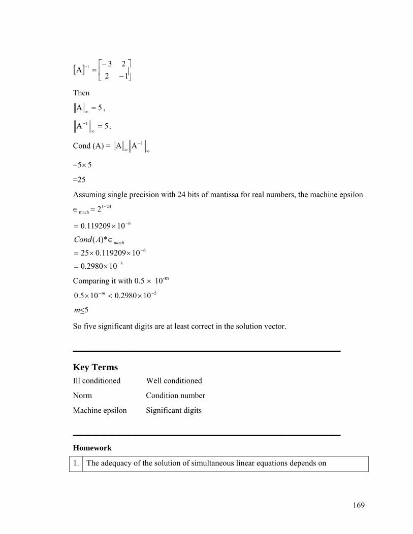
[ ] ⎥⎦
⎤⎢⎣
⎡−
−=−
1223
A 1
Then
5A =∞
,
5A 1 =∞
− .
∞
−∞
1AACond (A) =
=5×5
=25
Assuming single precision with 24 bits of mantissa for real numbers, the machine epsilon 241
mach 2 −=∈
610119209.0 −×=
5
6
102980.010119209.025
)*(
−
−
×=
××=
∈machACond
Comparing it with 0.5 × 10-m
5102980.0105.0 −− ×<× m
5<m
So five significant digits are at least correct in the solution vector.
_________________________________
Key Terms Ill conditioned Well conditioned
Norm Condition number
Machine epsilon Significant digits
_________________________________
Homework
1. The adequacy of the solution of simultaneous linear equations depends on
169

A. Condition number
B. Machine epsilon
C. Product of condition number and machine epsilon
D. Norm of the matrix.
2.
If a system of equations [A] [X] = [C] is ill conditioned, then
A. det(A) = 0
B. Cond(A) = 1
C. Cond(A) is large.
A is large. D.
If Cond(A) = 104 and = 0.119 × 10⁻⁶mach∈ , then in [A] [X] = [C], at least these many
significant digits are correct in your solution,
A. 3
B. 2
C. 1
D. 0
3.
Make a small change in the coefficient matrix to
⎥⎦
⎤⎢⎣
⎡=⎥
⎦
⎤⎢⎣
⎡⎥⎦
⎤⎢⎣
⎡999.74
yx
999.3221
and find
∞∞
∞∞
Δ
Δ
A/AX/X
Is it a large or small number? How is this number related to the condition number of the matrix?
170

4.
Make a small change in the coefficient matrix to
⎥⎦
⎤⎢⎣
⎡=⎥
⎦
⎤⎢⎣
⎡⎥⎦
⎤⎢⎣
⎡74
yx
3221
and find
∞∞
∞∞
Δ
Δ
A/AX/X
Is it a large or a small number? Compare your results with the previous problem. How is this number related to the condition number of the matrix?
5. Prove
CC
AAXX 1 Δ
<Δ −
6.
For
[ ]⎥⎥⎥
⎦
⎤
⎢⎢⎢
⎣
⎡
−−
−=
5156099.230710
A
gives
[ ]⎥⎥⎥
⎦
⎤
⎢⎢⎢
⎣
⎡
×−−−−
=−
−
5
1
10664.61666.004995.03999.03332.02999.02799.02333.01099.0
A
a) What is the condition number of [A]?
b) How many significant digits can we at least trust in the solution of [ ][ ] [ ]CXA = if 6
mach 101192.0 −×=∈
c)Without calculating the inverse of the matrix [A], can you estimate the condition
171
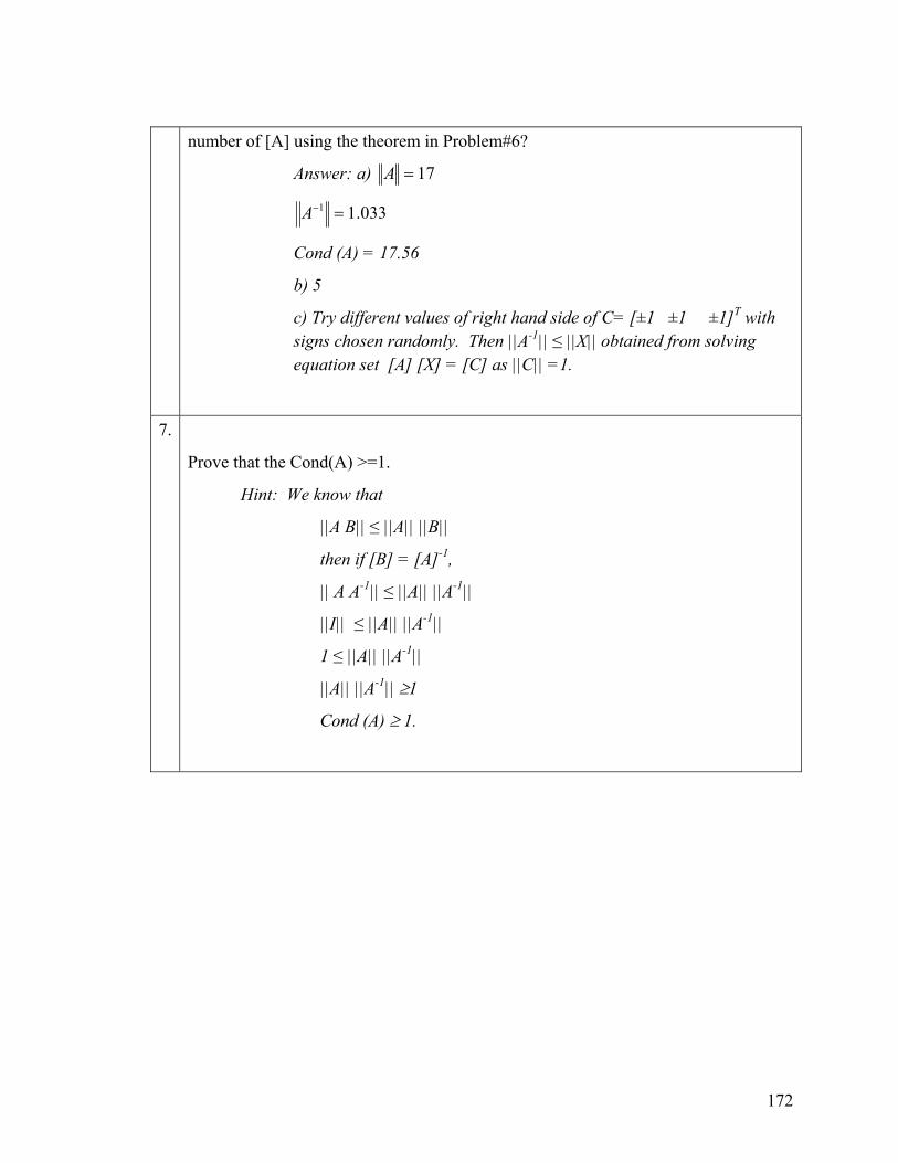
number of [A] using the theorem in Problem#6?
17=A Answer: a)
033.11 =−A
Cond (A) = 17.56
b) 5 Tc) Try different values of right hand side of C= [±1 ±1 ±1] with
signs chosen randomly. Then ||A-1|| ≤ ||X|| obtained from solving equation set [A] [X] = [C] as ||C|| =1.
7.
Prove that the Cond(A) >=1.
Hint: We know that
||A B|| ≤ ||A|| ||B|| -1, then if [B] = [A]
|| A A-1|| ≤ ||A|| ||A-1||
||I|| ≤ ||A|| ||A-1||
1 ≤ ||A|| ||A-1||
||A|| ||A-1|| ≥1
Cond (A) ≥ 1.
172
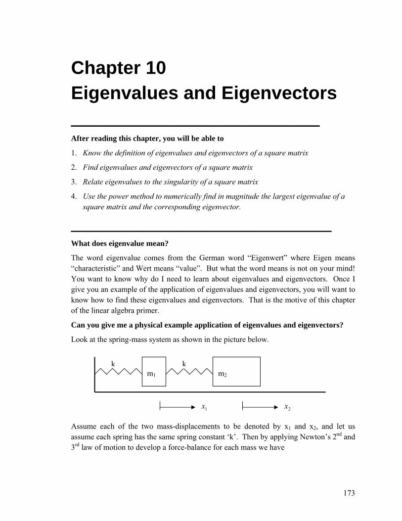
Chapter 10 Eigenvalues and Eigenvectors ___________________________ After reading this chapter, you will be able to
1. Know the definition of eigenvalues and eigenvectors of a square matrix
2. Find eigenvalues and eigenvectors of a square matrix
3. Relate eigenvalues to the singularity of a square matrix
4. Use the power method to numerically find in magnitude the largest eigenvalue of a square matrix and the corresponding eigenvector.
_________________________________
What does eigenvalue mean?
The word eigenvalue comes from the German word “Eigenwert” where Eigen means “characteristic” and Wert means “value”. But what the word means is not on your mind! You want to know why do I need to learn about eigenvalues and eigenvectors. Once I give you an example of the application of eigenvalues and eigenvectors, you will want to know how to find these eigenvalues and eigenvectors. That is the motive of this chapter of the linear algebra primer.
Can you give me a physical example application of eigenvalues and eigenvectors?
Look at the spring-mass system as shown in the picture below.
1x 2x
m1
m2
k k
Assume each of the two mass-displacements to be denoted by x1 and x2, and let us assume each spring has the same spring constant ‘k’. Then by applying Newton’s 2nd and 3rd law of motion to develop a force-balance for each mass we have
173
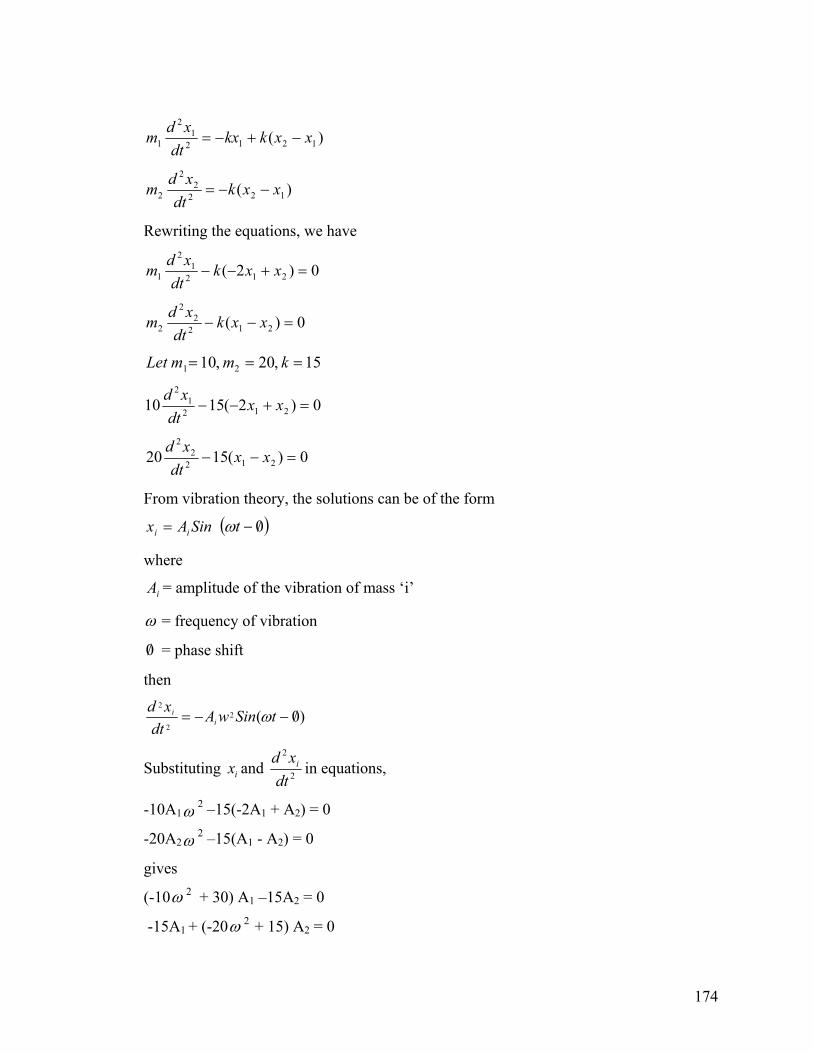
)( 12121
2
1 xxkkxdt
xdm −+−=
)( 1222
2
2 xxkdt
xdm −−=
Rewriting the equations, we have
0)2( 2121
2
1 =+−− xxkdt
xdm
0)( 2122
2
2 =−− xxkdt
xdm
15 ,20 ,10 21 === kmmLet
0)2(1510 2121
2
=+−− xxdt
xd
0)(1520 2122
2
=−− xxdt
xd
From vibration theory, the solutions can be of the form
( )0/−tωSinAx ii =
where
iA = amplitude of the vibration of mass ‘i’
ω = frequency of vibration
0/ = phase shift
then
)0(22
2
/−−= tSinwAdt
xdi
i ω
2
2
dtxd iSubstituting and ix in equations,
-10A1ω 2 –15(-2A1 2 + A ) = 0
-20A2ω 2 –15(A1 2 - A ) = 0
gives
(-10ω 2 + 30) A –15A = 0 1 2
-15A1 + (-20ω 2 + 15) A = 0 2
174
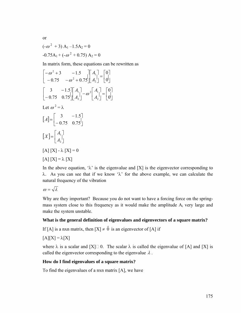
or
(-ω 2 + 3) A –1.5A = 0 1 2
-0.75A1 + (-ω 2 + 0.75) A = 0 2
In matrix form, these equations can be rewritten as
⎥⎦
⎤⎢⎣
⎡=⎥
⎦
⎤⎢⎣
⎡⎥⎦
⎤⎢⎣
⎡
+−−−+−
00
75.075.05.13
2
12
2
AA
ωω
⎥⎦
⎤⎢⎣
⎡=⎥
⎦
⎤⎢⎣
⎡−⎥
⎦
⎤⎢⎣
⎡⎥⎦
⎤⎢⎣
⎡−
−00
75.075.05.13
2
12
2
1
AA
AA
ω
Let ω 2 = λ
[ ] ⎥⎦
⎤⎢⎣
⎡−
−=
75.075.05.13
A
[ ] ⎥⎦
⎤⎢⎣
⎡=
2
1
AA
X
[A] [X] - λ [X] = 0
[A] [X] = λ [X]
In the above equation, ‘λ’ is the eigenvalue and [X] is the eigenvector corresponding to λ. As you can see that if we know ‘λ’ for the above example, we can calculate the natural frequency of the vibration
λω =
Why are they important? Because you do not want to have a forcing force on the spring-mass system close to this frequency as it would make the amplitude Ai very large and make the system unstable.
What is the general definition of eigenvalues and eigenvectors of a square matrix?
If [A] is a nxn matrix, then [X] ≠ 0r
is an eigenvector of [A] if
[A][X] = λ[X]
where λ is a scalar and [X] 0. The scalar λ is called the eigenvalue of [A] and [X] is called the eigenvector corresponding to the eigenvalue λ .
How do I find eigenvalues of a square matrix?
To find the eigenvalues of a nxn matrix [A], we have
175

[A][X] = λ[X]
[A][X] - λ[X] = 0
[A][X] - λ[I][X] = 0
([A] - λ[I])[X] = 0
Now for the above set of equations to have a nonzero solution,
det ([A] - λ[I]) = 0
This left hand side can be expanded to give a polynomial in λ solving the above equation would give us values of the eigenvalues. The above equation is called the characteristic equation of [A].
For a nxn [A] matrix, the characteristic polynomial of A is of degree n as follows
det ([A] - λ[I]) = 0
gives
λn n-1 + c λ + - - + c1 n = 0
Hence this polynomial can have n roots.
_________________________________
Example
Find the eigenvalues of the physical problem discussed in the beginning of this chapter, that is, find the eigenvalues of the matrix
[ ] ⎥⎦
⎤⎢⎣
⎡−
−=
75.075.05.13
A
Solution
[ ] [ ] ⎥⎦
⎤⎢⎣
⎡−−
−−=−
λλ
λ75.075.0
5.13IA
[ ] [ ] 0)5.1)(75.0()75.0)(3()det( =−−−−−=− λλλ IA
0125.1375.025.2 2 =−+−− λλλ
0125.175.32 =+− λλ
)1(2)125.1)(1(4)75.3()75.3( 2 −−±−−
=λ
176

2092.375.3 ± =
=3.421,0.3288
So the eigenvalues are 3.421 and 0.3288.
_________________________________
Example
Find the eigenvectors of
⎥⎦
⎤⎢⎣
⎡−
−=
75.075.05.13
A
Solution
The eigenvalues have already been found in the previous example
3288.0,421.3 21 == λλ
Let
[ ] ⎥⎦
⎤⎢⎣
⎡=
2
1
xx
X
be the eigenvector corresponding to
421.31 =λ
Hence
( [ - λ]A 1 [I]) [ = 0 ]X
01001
421.375.075.0
5.13
2
1 =⎥⎦
⎤⎢⎣
⎡
⎭⎬⎫
⎩⎨⎧
⎥⎦
⎤⎢⎣
⎡−⎥
⎦
⎤⎢⎣
⎡−
−xx
⎥⎦
⎤⎢⎣
⎡=⎥
⎦
⎤⎢⎣
⎡⎥⎦
⎤⎢⎣
⎡−−−−
00
671.275.05.1421.0
2
1
xx
If
1x = s
Then
-0.421s-1.5 =0 2x
177

= -0.2807 s 2x
421.31 =λThe eigenvector corresponding to then is
⎥⎦
⎤⎢⎣
⎡−
=⎥⎦
⎤⎢⎣
⎡−
=2807.01
2807.0][ s
ss
X .
The eigenvector corresponding to 421.31 =λ is ⎥⎦
⎤⎢⎣
⎡− 2807.0
1
3288.02 =λ is Similarly, the eigenvector corresponding to
⎥⎦
⎤⎢⎣
⎡781.11
_________________________________
Example
Find the eigenvalues and eigenvectors of
[ ]⎥⎥⎥
⎦
⎤
⎢⎢⎢
⎣
⎡
−−−=
005.05.05.05.0
105.1A
Solution
The characteristic equation is given by
det ( [ - λ[ ) = 0 ]A ]I
005.0
5.05.05.0105.1
det =⎥⎥⎥
⎦
⎤
⎢⎢⎢
⎣
⎡
−−−−−
−
λλ
λ
( ) 0)]5.0)(5.0()0)(5.0[(1)]0)(5.0())(5.0)[(5.1( =−−−−+−−−−− λλλλ
025.025.12 23 =+−+− λλλ
The roots of the above equation are
0.1 ,5.0 ,5.0=λ
Note that there are eigenvalues that are repeated. Since there are only two distinct eigenvalues, there are only two eigenspaces. But corresponding to λ = 0.5 there should be two eigenvectors that form a basis for the eigenspace.
178
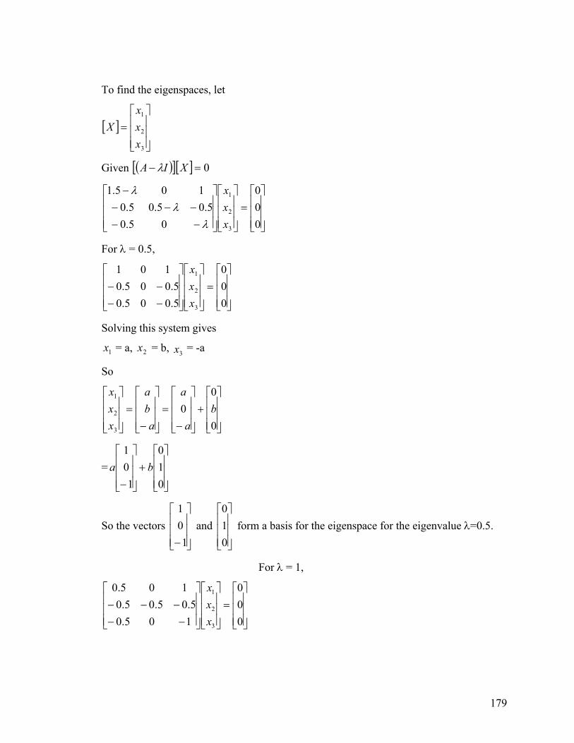
To find the eigenspaces, let
[ ]⎥⎥⎥
⎦
⎤
⎢⎢⎢
⎣
⎡=
3
2
1
xxx
X
( )[ ][ ] 0 =− XIA λGiven
⎥⎥⎥
⎦
⎤
⎢⎢⎢
⎣
⎡=
⎥⎥⎥
⎦
⎤
⎢⎢⎢
⎣
⎡
⎥⎥⎥
⎦
⎤
⎢⎢⎢
⎣
⎡
−−−−−
−
000
05.05.05.05.0
105.1
3
2
1
xxx
λλ
λ
For λ = 0.5,
⎥⎥⎥
⎦
⎤
⎢⎢⎢
⎣
⎡=
⎥⎥⎥
⎦
⎤
⎢⎢⎢
⎣
⎡
⎥⎥⎥
⎦
⎤
⎢⎢⎢
⎣
⎡
−−−−
000
5.005.05.005.0
101
3
2
1
xxx
Solving this system gives
1x = a, = b, = -a 2x3x
So
⎥⎥⎥
⎦
⎤
⎢⎢⎢
⎣
⎡+
⎥⎥⎥
⎦
⎤
⎢⎢⎢
⎣
⎡
−=
⎥⎥⎥
⎦
⎤
⎢⎢⎢
⎣
⎡
−=
⎥⎥⎥
⎦
⎤
⎢⎢⎢
⎣
⎡
0
00
3
2
1
ba
a
aba
xxx
= ⎥⎥⎥
⎦
⎤
⎢⎢⎢
⎣
⎡+
⎥⎥⎥
⎦
⎤
⎢⎢⎢
⎣
⎡
− 010
101
ba
So the vectors and form a basis for the eigenspace for the eigenvalue λ=0.5. ⎥⎥⎥
⎦
⎤
⎢⎢⎢
⎣
⎡
010
⎥⎥⎥
⎦
⎤
⎢⎢⎢
⎣
⎡
−101
For λ = 1,
⎥⎥⎥
⎦
⎤
⎢⎢⎢
⎣
⎡=
⎥⎥⎥
⎦
⎤
⎢⎢⎢
⎣
⎡
⎥⎥⎥
⎦
⎤
⎢⎢⎢
⎣
⎡
−−−−−
000
105.05.05.05.0
105.0
3
2
1
xxx
179
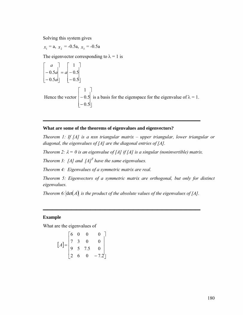
Solving this system gives
= a, = -0.5a, = -0.5a 1x 2x 3x
The eigenvector corresponding to λ = 1 is
⎥⎥⎥
⎦
⎤
⎢⎢⎢
⎣
⎡
−−=
⎥⎥⎥
⎦
⎤
⎢⎢⎢
⎣
⎡
−−
5.05.0
1
5.05.0 aaa
a
Hence the vector is a basis for the eigenspace for the eigenvalue of λ = 1. ⎥⎥⎥
⎦
⎤
⎢⎢⎢
⎣
⎡
−−
5.05.0
1
_________________________________
What are some of the theorems of eigenvalues and eigenvectors?
Theorem 1: If [A] is a nxn triangular matrix – upper triangular, lower triangular or diagonal, the eigenvalues of [A] are the diagonal entries of [A].
Theorem 2: λ = 0 is an eigenvalue of [A] if [A] is a singular (noninvertible) matrix. T have the same eigenvalues. Theorem 3: [A] and [A]
Theorem 4: Eigenvalues of a symmetric matrix are real.
Theorem 5: Eigenvectors of a symmetric matrix are orthogonal, but only for distinct eigenvalues.
( )Adet is the product of the absolute values of the eigenvalues of [A]. Theorem 6:
_________________________________
Example
What are the eigenvalues of
[ ]⎥⎥⎥⎥
⎦
⎤
⎢⎢⎢⎢
⎣
⎡
−
=
2.706205.75900370006
A
180
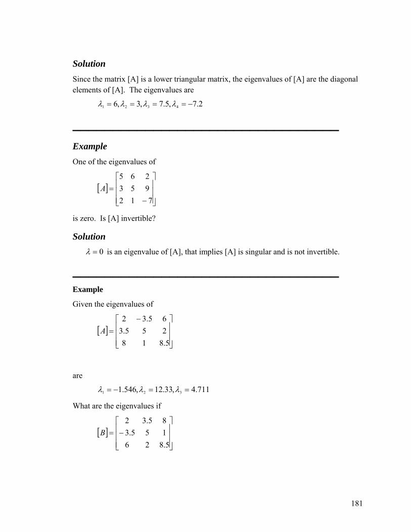
Solution Since the matrix [A] is a lower triangular matrix, the eigenvalues of [A] are the diagonal elements of [A]. The eigenvalues are
2.7,5.7,3,6 4321 −==== λλλλ
_________________________________
Example One of the eigenvalues of
[ ]⎥⎥⎥
⎦
⎤
⎢⎢⎢
⎣
⎡
−=
712953265
A
is zero. Is [A] invertible?
Solution 0=λ is an eigenvalue of [A], that implies [A] is singular and is not invertible.
_________________________________
Example
Given the eigenvalues of
[ ]⎥⎥⎥
⎦
⎤
⎢⎢⎢
⎣
⎡ −=
5.818255.365.32
A
are
711.4,33.12,546.1 321 ==−= λλλ
What are the eigenvalues if
[ ]⎥⎥⎥
⎦
⎤
⎢⎢⎢
⎣
⎡−=
5.826155.385.32
B
181

Solution Since [B] = [A]T, the eigenvalues of [A] and [B] are the same. Hence eigenvalues of [B] also are
711.4,33.12,546.1 321 ===− λλλ
Example Given the eigenvalues of
[ ]⎥⎥⎥
⎦
⎤
⎢⎢⎢
⎣
⎡ −=
0.818255.365.32
A
are
711.4,33.12,546.1 321 ==−= λλλ
Calculate the magnitude of the determinant of the matrix.
Solution Since
[ ] 321 det λλλ=A
4.711 12.33 546.1−=
= 89.80
_________________________________
How does one find eigenvalues and eigenvectors numerically?
One of the most common methods used for finding eigenvalues and eigenvectors is the power method. It is used to find the largest eigenvalue in absolute sense. Note that if this largest eigenvalues is repeated, this method will not work. Also this eigenvalue needs to be distinct. The method is as follows:
( )[ ]0X for the eigenvector in 1. Assume a guess
[A][X] = λ[X] ( )[ ]0Xequation. One of the entries of needs to be unity.
2. Find
182

[Y] (1) = [X[ ]A (0)]
3. Scale [Y(1)] so that the chosen unity component remains unity.
[Y(1) (1)] = λ [X(1)] ( )[ ]2X4. Repeat steps (2) and (3) with [X] = [X(1)] to get .
5. Repeat the setups 2 and 3 until the value of the eigenvalue converges. If s∈ is the pre-specified percentage relative error tolerance to which you would like the answer to converge to, keep iterating until
( ) ( )
( ) si
ii
ελ
λλ≤×
−+
+
1001
1
where the left hand side of the above inequality is the definition of absolute percentage relative approximate error, denoted generally by .aε A prespecified
percentage relative tolerance of implies at least significant digits are current in your answer. When the system converges, the value of λ is the largest (in absolute value) eigenvalue of [A].
''mm−× 2105.0
_________________________________
Example
Using the power method, find the largest eigenvalue and the corresponding eigenvector of
[ ]⎥⎥⎥
⎦
⎤
⎢⎢⎢
⎣
⎡
−−−=
005.05.05.05.0
105.1A
Solution
Assume
[ ]⎥⎥⎥
⎦
⎤
⎢⎢⎢
⎣
⎡=
111
)0(X
[ ][ ]⎥⎥⎥
⎦
⎤
⎢⎢⎢
⎣
⎡
⎥⎥⎥
⎦
⎤
⎢⎢⎢
⎣
⎡
−−−=
111
005.05.05.05.0
105.1 )0(XA
183

⎥⎥⎥
⎦
⎤
⎢⎢⎢
⎣
⎡
−−=
5.05.0
5.2
( )
⎥⎥⎥
⎦
⎤
⎢⎢⎢
⎣
⎡
−−=
2.02.0
15.21Y
(1) = 2.5 λ( )[ ]0XWe will choose the first element of to be unity.
[ ]⎥⎥⎥
⎦
⎤
⎢⎢⎢
⎣
⎡
−−=
2.02.0
1)1(X
[ ][ ]⎥⎥⎥
⎦
⎤
⎢⎢⎢
⎣
⎡
−−
⎥⎥⎥
⎦
⎤
⎢⎢⎢
⎣
⎡
−−−=
2.02.0
1
005.05.05.05.0
105.1 )1(XA
⎥⎥⎥
⎦
⎤
⎢⎢⎢
⎣
⎡
−−=
5.05.0
3.1
⎥⎥⎥
⎦
⎤
⎢⎢⎢
⎣
⎡
−−=
3846.03846.01
3.1][ )2(Y
(2) = 1.3 λ
[ ]⎥⎥⎥
⎦
⎤
⎢⎢⎢
⎣
⎡
−−=
3846.03846.01
)2(X
The absolute relative approximate error in the eigenvalues is
100|| )2(
)1()2(
xa λλλε −
=
1003.1
5.13.1 x−=
184
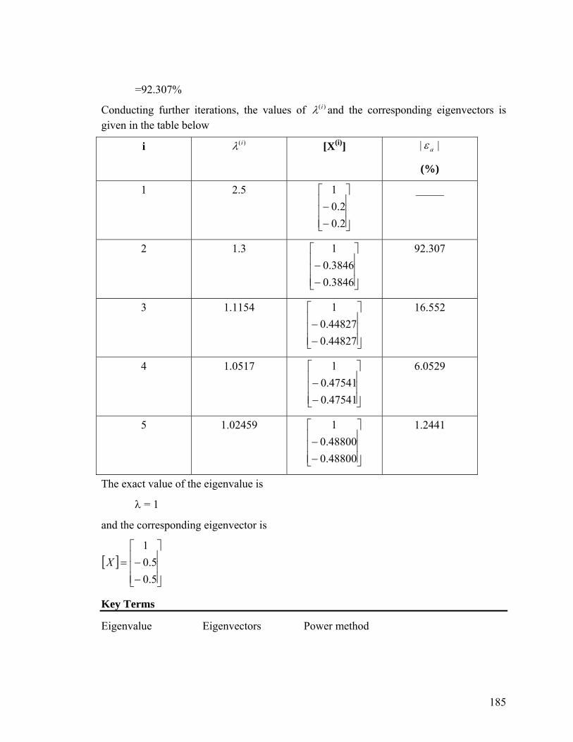
=92.307%
Conducting further iterations, the values of and the corresponding eigenvectors is given in the table below
)(iλ
i )(iλ [X(i) || aε]
(%)
1 2.5
⎥⎥⎥
⎦
⎤
⎢⎢⎢
⎣
⎡
−−
2.02.0
1 _____
2 1.3
⎥⎥⎥
⎦
⎤
⎢⎢⎢
⎣
⎡
−−
3846.03846.01 92.307
3 1.1154
⎥⎥⎥
⎦
⎤
⎢⎢⎢
⎣
⎡
−−
44827.044827.01 16.552
4 1.0517
⎥⎥⎥
⎦
⎤
⎢⎢⎢
⎣
⎡
−−
47541.047541.01 6.0529
5 1.02459
⎥⎥⎥
⎦
⎤
⎢⎢⎢
⎣
⎡
−−
48800.048800.01 1.2441
The exact value of the eigenvalue is
λ = 1
and the corresponding eigenvector is
[ ]⎥⎥⎥
⎦
⎤
⎢⎢⎢
⎣
⎡
−−=
5.05.0
1X
Key Terms
Eigenvalue Eigenvectors Power method
185

_________________________________
Homework 1.
The eigenvalues ‘λ’ of matrix [A] are found by solving the equation(s)? 0=− IA λ a)
b) [ ][ ] [ ]IXA =
c) [ ][ ] [ ] 0r
=− IXA λ0=Ad)
2. Find the eigenvalues and eigenvectors of
⎥⎦
⎤⎢⎣
⎡=
32910
][A
using the determinant method
Answer: (12,1), , ⎥⎦
⎤⎢⎣
⎡2169.09762.0
⎥⎦
⎤⎢⎣
⎡− 8381.0
8381.0
3.
Find the eigenvalues and eigenvectors of
⎥⎥⎥
⎦
⎤
⎢⎢⎢
⎣
⎡−=
102102104
][A
using the determinant method
Answer: (0,4,5615,0.43845), , , ⎥⎥⎥
⎦
⎤
⎢⎢⎢
⎣
⎡−
99068.05284.327816.0
⎥⎥⎥
⎦
⎤
⎢⎢⎢
⎣
⎡−
48963.027496.0
87193.0
⎥⎥⎥
⎦
⎤
⎢⎢⎢
⎣
⎡
010
4.
Find the eigenvalues of these matrices by inspection
186
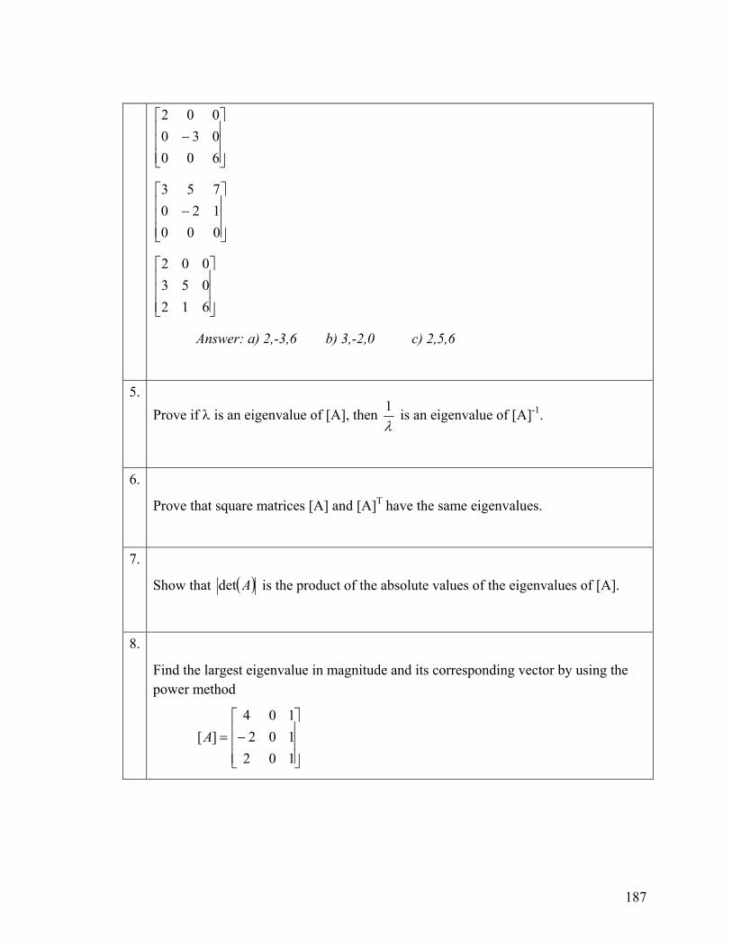
⎥⎥⎥
⎦
⎤
⎢⎢⎢
⎣
⎡−
600030002
⎥⎥⎥
⎦
⎤
⎢⎢⎢
⎣
⎡−
000120753
⎥⎥⎥
⎦
⎤
⎢⎢⎢
⎣
⎡
612053002
Answer: a) 2,-3,6 b) 3,-2,0 c) 2,5,6
5.
λ1 is an eigenvalue of [A]-1. Prove if λ is an eigenvalue of [A], then
6.
Prove that square matrices [A] and [A]T have the same eigenvalues.
7.
( )Adet is the product of the absolute values of the eigenvalues of [A]. Show that
8.
Find the largest eigenvalue in magnitude and its corresponding vector by using the power method
⎥⎥⎥
⎦
⎤
⎢⎢⎢
⎣
⎡−=
102102104
][A
187

Start with an initial guess of the eigenvector as ⎥⎥⎥
⎦
⎤
⎢⎢⎢
⎣
⎡−
5.05.0
1
Answer:4.5615, after 4 iterations
⎥⎥⎥
⎦
⎤
⎢⎢⎢
⎣
⎡−
56154.031534.01
188

INDEX
A
Addition of matrices · 51Addition of vectors · 37adjoint · 93, 94, 98Associate law of addition · 49Associate law of multiplication · 49associative law of multiplication · 49augmented matrix · 78, 80, 81, 82, 83, 84, 85, 86
B
back substitution · 114, 116, 118, 128, 130Back Substitution · 108, 109
C
cofactor · 55, 59, 67, 69, 94, 98column vector · 8, 9, 16, 20, 21, 24, 56Column vector · 8Commutative law of addition · 49condition number · 5, 161, 166, 170, 171, 172 Condition number · 170conditioning of the matrix · 5, 6, 158, 162, 166 consistent · 4, 5, 74, 77, 78, 79, 80, 82, 83, 84, 85, 86, 96, 97 Consistent · 5, 86, 95
D
decompose a non-singular matrix · 5, 131 determinant · 4, 5, 55, 59, 60, 63, 64, 65, 66, 67, 68, 69, 71, 72, 78, 80, 81, 82, 83, 102, 107, 122, 123, 125, 126, 127,
161, 183, 187Determinant · 66, 102, 103, 124iagdonal · 4, 10, 11, 13, 14, 57, 58, 71, 100, 122, 124, 132, 144, 181Diagonal · 11, 16diagonal elements · 10, 11, 13, 57, 58, 71, 132, 144, 181diagonal matrix · 11, 100, 124Diagonal matrix · 11, 16diagonally dominant coefficient matrices · 150diagonally dominant matrix · 14, 15 Diagonally Dominant Matrix · 14distributive law · 52Distributive law · 4 9dot product · 4, 36, 37
E
eigenvalue · 6, 174, 176, 180, 181, 182, 183, 184, 186, 188
2

Eigenvalue · 186Eigenvalues · 6, 174, 181eigenvectors · 6, 174, 176, 178, 179, 181, 183, 185, 187Eigenvectors · 6, 174, 181, 186element of the matrix · 8elimination methods · 131Elimination methods · 5, 122, 144entry · 8, 31, 59, 93, 94Equal matrices · 16
F
Forward substitution · 135, 138
G
Gauss · 5, 107, 113, 115, 118, 119, 122, 123, 124, 125, 126, 127, 128, 129, 131, 132, 135, 140, 144, 149, 150, 151, 153, 154, 155, 156, 157
Gauss Elimination · 5, 107, 113, 115, 118, 119, 122, 123, 124, 125, 126, 128, 129, 132Gaussian · 5, 107, 118, 119, 120, 123, 124, 125, 126, 127, 129, 130, 131, 132, 140, 142Gaussian elimination with partial pivoting · 5, 118, 119, 123, 124, 126Gauss-Siedel method · 144
I
identity matrix · 11, 12, 17, 52, 72, 124, 131, 137Identity matrix · 11, 16 ill conditioned · 5, 158, 159, 160, 161, 162, 166, 170 Ill conditioned · 170Inconsistent · 95inconsistent system · 5, 74, 77, 78, 79Inconsistent system · 95inverse of a matrix · 5, 74, 87, 88, 89, 92, 131invertible · 5, 87, 92, 99, 100, 101, 124, 126, 161, 182invertible matrix · 92
L
Linear combination · 33, 37, 51linear combination of matrices · 4, 48Linear combination of matrices · 51linear combination of vectors · 4, 20, 26, 36Linear combination of vectors · 37linearly dependent · 29, 31, 32, 33, 34, 39, 40, 106linearly independent · 4, 20, 27, 28, 29, 31, 32, 33, 34, 38, 39, 40, 87, 102, 105Linearly independent · 37lower triangular matrix · 10, 11, 17, 124, 129, 132, 181Lower triangular matrix · 10, 16LU · 5, 129, 130, 131, 132, 134, 136, 137, 140, 141, 142LU Decomposition · 5, 129, 131, 136
3

M
matrices · 4, 5, 7, 13, 14, 15, 16, 17, 41, 43, 44, 48, 49, 50, 51, 53, 54, 55, 59, 63, 67, 72, 76, 87, 92, 99, 100, 102, 122, 131, 140, 161, 165, 166, 167, 187, 188
Matrices · 7matrix · 4, 5, 7, 8, 9, 10, 11, 12, 13, 16, 43, 45, 46, 47, 48, 49, 51, 52, 53, 54, 55, 56, 57, 58, 59, 60, 63, 68, 69, 72, 74,
75, 76, 79, 80, 81, 82, 83, 84, 85, 86, 87, 88, 89, 90, 93, 94, 96, 98, 101, 102, 103, 105, 107, 112, 113, 116, 122, 123, 124, 126, 127, 129, 130, 131, 132, 133, 135, 136, 140, 142, 149, 150, 154, 158, 159, 160, 161, 165, 166, 170, 171, 172, 176, 177, 181, 183, 186
Matrix · 4, 7, 14, 16, 41, 51, 55, 74multiplication of matrices · 50Multiplication of matrices · 51
N
nonsingular matrix · 129, 131, 142nontrivial solution · 31, 33norm of the matrix · 158, 161Norm of the matrix · 170null · 4, 24, 34, 39Null · 37
P
power method · 174, 183, 184, 188principal · 10product of matrices · 51properties of norms · 5, 165
R
rank of a matrix · 5, 78row vector · 8, 16, 20, 47, 56Row vector · 8
S
singular · 87, 181, 182Singular · 126skew-symmetric matrix · 4, 56, 67, 71special types of matrices · 4, 7, 8square matrix · 4, 5, 6, 9, 10, 11, 13, 14, 16, 19, 55, 56, 59, 87, 88, 95, 107, 122, 123, 136, 140, 142, 161, 174, 176Square matrix · 9, 16submatrix · 9, 59, 78, 79, 80, 81, 82, 83Submatrix · 9Subtraction of matrices · 51symmetric matrix · 56, 57, 67, 71, 141, 181 Symmetric matrix · 56system of equations · 4, 5, 74, 77, 78, 80, 82, 83, 84, 85, 86, 96, 97, 103, 128, 144, 149, 150, 153, 154, 155, 156, 157,
158, 159, 160, 161, 162, 164, 166, 168, 169, 170System of Equations · 4, 74
4
T
trace of a matrix · 55Trace of a matrix · 57transpose · 55, 56, 58, 70Transpose · 55, 66Tridiagonal matrices · 13
U
unique solution · 5, 40, 74, 77, 84, 86, 95, 96, 97, 101, 124Unique solution · 95unit · 4, 24, 40Unit · 37Unit vector · 37upper triangular matrix · 10, 17, 66, 71, 123, 124, 129, 132Upper triangular matrix · 10, 16
V
vector · 4, 6, 8, 9, 20, 23, 24, 25, 26, 31, 34, 35, 37, 39, 40, 56, 76, 80, 89, 112, 131, 134, 136, 147, 148, 149, 153, 159, 160, 161, 162, 163, 164, 165, 166, 167, 168, 169, 170, 181, 188
Vector · 8, 16, 37
W
well-conditioned · 5, 159, 164, 166
Z
zero matrix · 12Zero matrix · 12, 16zero vector · 24, 30, 32, 40, 105
5