Introduction to Mechanical Testing for Engineering

Science Students

Jeffrey W. Kysar

September 30, 2009

1 Introduction

Experimental measurement of the mechanical behavior of structures and systems is very

important for design, validation of theories and well as lifetime estimates. This document

gives a brief overview the measurement of several aspects of mechanical behavior, including:

the definitions of different stress and strain measures; discussion of elastic properties; mea-

surement of the elastic and plastic properties using a Universal Testing Machine; an overview

of strain gages; and finally, a discussion of the Wheatstone Bridge.

2 Definitions of Stress and Strain

Stress is a measure used to quantify the force transmitted through an object on a per

unit area basis; as such, it has a units of force per area. Strictly speaking, stress is a tensor

quantity which is a generalization of a vector quantity. A vector quantity (such as force) has

a magnitude and a direction associated with it. A tensor quantity (of the type of stress or

strain) has three magnitudes and three directions associated with it; the three magnitudes

are known as principal stresses (or strains) and the three directions are known as principal

1

axes. Thus, six pieces of information (i.e. numbers) are required to fully describe the stress

(or strain) state at each point within an object.

We will consider the the stress state associated with a rod of uniform cross-section sus-

pended from a ceiling with a weight that exerts a force of magnitude P hanging from its

lower end. We learn in elementary Physics that we can express—or find numerical values

for the coefficients of—a vector using any set of coordinate axes we choose; however we also

learn that some coordinate axes are more convenient to use than others. In the case we are

considering, the most convenient set of coordinate axes has one axis (i.e. the x-axis, the

y-axis or the z-axis) coincident with the central axis of the rod. For example, if the y-axis is

chosen to be along the rod’s axis (with mutually perpendicular x-axis and z-axis), the force

vector can be expressed as P = (0, P, 0). Since the rod is stationary, the magnitude P does

not vary along the length of the rod. (Otherwise one portion of the rod would accelerate

relative to the other portions. This would occur if we were, say, to hit the end of the rod

with a hammer.) Thus only one coefficient of the force vector is non-zero and furthermore

it is constant; we refer to this type of load (i.e. force) on the bar as being uni-axial.

Before defining the stress, we must first define an appropriate cross-sectional area of the

rod. To begin, we will choose to characterize the cross-sectional area that is perpendicular

to the axis of the bar, so that a unit normal vector to the cross-section is parallel to the axis

of the rod. Afterward we must choose when we measure the area. One obvious choice is

to measure the cross-sectional area prior to the application of the force P ; this area will be

denoted as A0. From experience or intuition we may expect the cross-sectional area of the

rod to change as the force is applied. Therefore, another obvious choice is to measure the

cross-sectional area after the application of the force P ; this area will be denoted as A. It

is clear that any number of other definitions for area could be chosen that are intermediate

between A0 and A.

The nominal stress (sometimes called engineering stress) is defined as

2

PA

L

A0

L0

a) b)

Figure 1: Uni-axial strain state: (a) Prior to application of load; (b) After application ofload.

σnom =P

A0. (1)

It is the most convenient stress measure for this experimental set-up because it is not neces-

sary to measure the area during loading.

However Newton’s Laws must be satisfied in the loaded configuration, (i.e. after the

forces have been applied) so a more fundamental stress measure is the true, or Cauchy,

stress defined as

σtrue =P

A= σnom

A0

A

, (2)

One important thing to notice is that the two different stress measures can be converted one

to the other. Therefore, from the perspective of calculation, it is important to choose one

stress measure and to apply it consistently.

Strain is a measure of the change in length of the rod on a per unit length basis. With

reference to Fig. 1, we define the initial length of the rod to be L0 and the length of the rod

after the force has been applied is denoted as L. The change in length is ∆L = L − L0.

An important related quantity is the so-called stretch ratio denoted as λ = L/L0. It in now

3

necessary to normalize ∆L to define the strain measure.

One clear option is to normalize with L0 which gives rise to a measure that is called the

nominal strain (sometimes called engineering strain) defined as

εnom =L− L0

L0=

∆L

L0= λ− 1. (3)

The corresponding “true”, or logarithmic, strain uses the current length L. However the

value of L changes continuously during the process of loading, so the true strain must be

calculated as the sum of an infinite number of infinitesimal strains calculated relative to the

current length. It is therefore defined as

εtrue =

L

L0

dL

L= ln

L

L0

= ln(λ). (4)

There are many other strain measures that can be defined. All valid strain measures, how-

ever, must be expressed solely as a function, f(λ), of the stretch ratio, λ. It must satisfy

f(1) = 0 which simply requires that the value of strain be zero relative to the reference state

(usually the undeformed object). In addition f (1) = 1, where the prime denotes differenti-

ation with respect to stretch ratio. This ensures that the function for strain is linear with

respect to stretch ratio for sufficiently small deformations. Another common condition is

that f (λ) > 0 which ensures that the strain increases monotonically with stretch ratio; this

condition is appropriate for the convention that an increase in length signifies a positive,

rather then a negative, strain. Since εnom is the only linear function which satisfies these

three conditions, all other strain measures must be non-linear functions in λ which reduce

to the nominal strain measure for sufficiently small values of strain.

The nominal strain measure is valid only for very small strain magnitudes, so small

in fact, that the strains are typically said to be small strain or infinitesimal strain. (The

term “infinitesimal” in this context simply refers to very small values, and is different than

4

the usage of the term “infinitesimal” in the context of calculus.) The true strain, along

with several other commonly used non-linear strain measures, are intended to be used in

circumstances in which the deformations are relatively large, or as is commonly said, for

finite strain conditions.

What are typical magnitudes of the deformation encountered in practice? Materials such

as many biological tissues and polymers can undergo very large stretch ratios on the order of

2 or 3 or greater (think of stretching your skin, a rubber band or a balloon). Special stress

and strain measures have been devised for these materials which are beyond the scope of

the discussion herein. Most conventional engineering materials (i.e. metals, cement, rock,

wood, ceramics, etc.) are used in designs for which the strain as well as the change in cross-

sectional area are no greater than about 0.1%. Under these circumstances, the difference

between A0 and A becomes negligible so all stress measures can be used interchangeably.

Thus the stress can be denoted simply as σ, where σ σnom σtrue, as is evident from

Equation 2. Likewise for strain, we can expand the function for true strain into a Taylor

series about λ = 1 to obtain εtrue = ln(λ) = (λ − 1) − 12(λ − 1)2 + · · · , which formally

converges for |λ− 1| ≤ 1. However we note that the first term of the expansion is identical

to the expression for εnom when (λ − 1)2 1. (The notation means “much, much less

than.”) Therefore, as with the stress state, the strain under these conditions can be denoted

simply as ε, where ε εnom εtrue.

Most machines and structures are designed so the material in their components remains

elastic as forces or displacements are applied. The term elastic implies that the applied

deformations are reversible in the sense that the object returns to the original configuration

of its unloaded state after the forces are removed (think of a spring that is pulled slightly

and then reverts to it original shape and size after the force is removed). If the applied

forces are sufficiently large, though, the material is permanently deformed (think of pulling

the spring so far that you put a permanent set in it such that the spring is somewhat longer

after unloading than it was before loading). The difference in the shape of the body before

5

and after the loading is attributed to plastic deformation.

Most common engineering materials remain elastic as long as the strains are less than

about ε 10−3 = 0.1%. As such, within the elastic range, the nominal stress and the nominal

strain measures are usually employed. In such a circumstance, even though, σ σnom σtrue

and ε εnom εtrue, it is good practice to report precisely which stress and strain measures

are employed.

Since there are many stress and strain measures that can be used for calculations, how

does one choose which strain measure to use with a given stress measure, or vice versa? We

use energy arguments to answer this. The fundamental definition of work is the application

of a force acting through a distance. In mathematical terms, the scalar quantity work, W ,

is expressed as W = F · D, where F refers to a constant force vector and D refers to a

constant displacement vector that the force acts along. When the force and displacement

vectors are not constants, then the appropriate definition for work is dW = F · dD, where

dW is an infinitesimal (this time in the context of the calculus) increment of work and dD,

is an infinitesimal increment of displacement.

Since stress is related to force and strain is related to displacement, we expect it is

possible to express the work as a function of stress and strain directly. Therefore, we write

the expression

dw = σw · dεw (5)

where dw will be some quantity related to dW , and the subscripts on σw and εw simply

denote a matching pair of stress and strain measures, respectively. (The dot product is

also a valid operation on tensor quantities such as stress and strain.) We first consider the

nominal stress and strain measures. We set σw = σnom = P/A0 from Eq. 1. Likewise, we

can set εw = εnom = λ − 1 from Eq. 3. The derivative of nominal strain with respect to

λ is dεw/dλ = 1, which can be rearranged to obtain the expression dεw = dλ . From the

definition of the stretch ratio, λ = L/L0, we find that dλ = dL/L0, since L0 is a constant.

6

Thus, dεw = dL/L0. Upon substitution of these expressions into Eq. 5 and noting that the

stress and strain act in the same direction, there results the following

dwnom =P

A0

dL

L0=

PdL

A0L0=

PdL

V0(6)

where V0 = A0L0 is the volume of the rod prior to the application of any load. Also we note

that the quantity PdL is simply the scalar form of the dW = F · dD so that PdL can be

interpreted as a small increment of work that the applied force exerts on the suspended rod.

Thus, the proper interpretation of dwnom in Eq. 6 is the work done on the suspended rod

per unit volume of the rod in its reference, unloaded configuration.

It is evident now that σnom and εnom are paired quantities that can be used to calculate

work; such stress and strain pairs are said to be work conjugate. Furthermore, the work is

calculated on a per unit volume basis. It should be emphasized, though, that the volume

used for the normalization will not always be that of the reference, unloaded configuration.

Finally, we see that the quantities, σw and εw used in Eq. 5 refer generically to work conjugate

pairs of stress and strain measures.

We next demonstrate that the σtrue and εtrue are also work conjugate measures. We

set σw = σtrue = P/A from Eq. 2. Likewise, we set εw = εtrue = ln(λ) from Eq. 4. The

derivative dεw/dλ = 1/λ can be rearranged to obtain the expression dεw = dλ/λ. Recalling

that dλ = dL/L0 leads to dεw = dL/L. Upon substitution of these expressions into Eq. 5

there results the following

dwtrue =P

A

dL

L=

PdL

AL=

PdL

V(7)

where V = AL is the current volume of the rod after the application of the force P . Thus,

the proper interpretation dwtrue in Eq. 7 is the work done on the suspended rod per unit

volume of the rod in its current, loaded configuration.

The discussion in this section has assumed a uni-axial stress state. These concepts are

7

readily extended to account for a fully general and arbitrary stress and strain state, which

are beyond the scope of this class. Students interested in learning more about topics related

to stress, strain and deformation should take Solid Mechanics courses or Elasticity courses

in as upper level electives or at graduate school.

3 Elastic Properties

The response of a material to an applied load is classified according to whether it remains

elastic or enters the elastic-plastic regime. If magnitude of the stress state stays below a

threshold known as the yield stress (or yield strength), the material is said to be elastic.

Atoms in a material which deforms elastically change their interatomic distances, but the

atoms retain the same nearest neighbors. Such a material stores elastic energy as it is

deformed that can be released upon unloading. In that sense, the system is thermodynami-

cally reversible. However if the applied stress exceeds the yield stress, the deformation occurs

simultaneously by two mechanisms: interatomic stretching due to elastic strain; and, inter-

change of atomic nearest neighbors resulting in mass flux due to plastic strain (in essence

the atoms flow through the crystal lattice analogously to fluid flow). If plastic deformation

occurs, the system is thermodynamically irreversible, so energy is dissipated. In essence, the

portion of the applied work that goes into elastic deformation is stored in the system, but

the portion of the applied work that goes into plastic deformation is dissipated.

3.1 Hooke’s Law

Stress and strain measures are, in-general, tensor quantities. The relationship between the

stress and strain measures during elastic deformation is known as Hooke’s Law. In this

course, we will only consider stress states that are either uni-axial or bi-axial. In the uni-

axial stress state discussed above, there was only one stress and one strain to consider. It

is not surprising, then, that there are two stresses and two strains that must be taken into

account for a bi-axial stress state. Examples of a bi-axial stress state include the walls of

8

y!

y!

x! x!

Figure 2: Bi-axial stress state

a cylindrical pressure vessel (think of a pressurized soda can), the stresses in an inflated

spherical balloon, etc.

As illustrated in Fig. 2, we adopt the following notation: σx is the normal stress that acts

in the direction of the x-axis; and, σy is the normal stress that acts in the direction of the

y-axis. Likewise for strains: εx is the normal strain that acts in the direction of the x-axis;

and, εy is the normal strain that acts in the direction of the y-axis. It is important to note

that there are no shear stresses (i.e. stresses that lead to changes of angle in Fig. 2 rather

than changes of lengths of the sides) considered in this special case.

For the case of the suspended rod discussed in Section 2, the relationship between stress

and strain for a uni-axial stress state is

σy = Eεy (8)

where E is a material property called the Young’s Modulus. Since strain measures are

dimensionless, E has the same units as stress. In addition to a deformation in the direction

of the y-axis, experiment also demonstrates that there is also deformation in the transverse

direction; in this case there is a normal strain in direction of the x-axis. This relationship is

9

quantified as

εx = −νεy (9)

where ν is known as Poisson’s ratio. This relationship shows that there is a coupling between

the normal strains in the x- and y-directions. The deformation is often called a Poisson

contraction, because if the suspended rod were to lengthen, its cross-sectional dimensions

would decrease according to Eq. 9.

When generalized to a bi-axial stress state, Hooke’s law is expressed as

εx = 1E (σx − νσy)

εy = 1E (σy − νσx)

(10)

which can be inverted to express the stresses in terms of the strains as

σx = E(1−ν2)(εx + νεy)

σy = E(1−ν2)(εy + νεx).

(11)

4 Measurement of Elastic and Plastic Properties

4.1 Universal Testing Machines

Many different types of testing equipment are used to measure the mechanical properties

of materials. One of the most versatile is the so-called Universal Testing Machine. These are

capable of testing a specimen in tension, compression, torsion and bending under a variety

of test conditions. During the test, the load, displacements, or strain of the specimen can be

accurately controlled while the other variables are being measured. Two leading companies

that manufacture universal testing machines are Instron Corporation and by MTS Systems

Corporation. These machines have a closed-loop control system and use a servo-hydraulic

or a servo-electric system to drive the test.

10

Figure 3: Schematic Representation of Universal Testing Machine (N.E. Dowling, MechanicalBehavior of Materials, p. 105, Prentice-Hall, 1999)

A representative sketch of a universal test machine is shown in Fig. 3. What follows is

a description of the capabilities of an Instron 8501 model.1The test specimen is mounted

between the upper part of the actuator and the lower part of the load cell. There are various

types of grips which are used to hold the specimen in position. The actuator drives the test

system by controlling the displacement of one end of the specimen. Physically, in the Instron

8501, the actuator is the ram of a hydraulic cylinder and its nominal full scale displacement is

±50 mm (2 in). A servo-valve allows the actuator to be accurately controlled. The position,

or stroke, of the actuator is measured with a linear variable differential transformer (LVDT).

The actuators of some other testing machines are screw-driven and are referred to as having

a servo-electric actuation. The load cell measures the force that is exerted on the specimen

during the test. The Instron 8501 has one load cell with a nominal 100 kN (22480 lbf) full

scale and another with a nominal 10 kN (2248 lbf) full scale. Each will measure a compressive

as well as tensile load to full scale.

The strain which the specimen experiences can be measured during the test. The Instron1The Mechanical Engineering Department will soon take delivery of a new Instron 5569A Table Mounted

Materials Testing System. Until that time, however, this discussion will make use of the Instron 8501 system

that the author used at a different university. However, in the lab this semester, we will use a servo-hydraulic

MTS system.

11

8501 has a strain gage with two knife edges that are placed in contact with the specimen

and secured in place with rubber bands. Assuming that the knife edges do not move relative

to the specimen during a test, the change in distance between the knife edges correspond to

the change in length. By knowing the initial length of the gage, the strain can be readily

calculated.

Another common method to measure the strain of a specimen is to use a resistance

strain gage. A resistance strain gage consists of a small metallic foil that is embedded in

a protective coating. The protective coating is glued onto a specimen. Under strains, the

resistance of the foil changes proportionally with the strain.

There are two crossheads. The fixed crosshead is always stationary with respect to

the actuator’s hydraulic cylinder. The adjustable crosshead can be moved up or down

with dedicated hydraulic cylinders to account for various testing needs. During a test, the

adjustable crosshead is locked into position. The crosshead is often abbreviated as x-head.

The outputs of the load cell, LVDT, and other gages are voltages between ±10 volts.

These voltages can be calibrated against their respective variables and measured with analog

or with digital data acquisition devices.

A control panel allows the testing machine to be operated manually. It has digital read

outs of the load, position, and strain in units which the user can specify. The user enters

commands at the control panel to control the motion of the actuator. In addition, the control

panel can be set to take appropriate actions when certain events are detected. For example,

if a certain load threshold is detected, the test can be paused by stopping the actuator.

Or after a certain number of cycles have occurred during a fatigue test, the test can be

terminated.

The main limitation of the control panel is that commands can not be stored and subse-

quently performed in a sequential manner. The operator must enter the commands at the

control panel throughout the test.

However, by using an auxiliary computer to control the Instron 8501, all commands

12

necessary to run a complete test can be entered into the computer and then transmitted to

the Instron 8501 at the correct time. The operator can use either a commercial software

package or a user-written program.

4.2 Control of the Universal Testing Machine

The goal of any test is to control one variable (independent variable) while measuring the

response of the other variables (dependent variables) which are pertinent to the system. The

Instron 8501 employs a digital feedback control loop to accurately control the independent

variable.

The testing machine can be controlled in three standard ways. Each method controls

the position of the actuator in order to control either the force exerted on the specimen,

the strain it experiences, or the displacement of one end of the specimen. In addition, some

testing machines allow control of other calculated variables such as true strain.

The independent variable can be controlled in a variety of wave forms. These include sine

waves, triangular waves, square waves, ramps, combinations of ramps, or a wave generated

externally. The amplitude and frequency of the wave forms can be varied within reasonable

limits.

To ensure the safety of the operator and of the testing machine, maximum limits on the

variables of the test can be set. If the position, load, or strain of the specimen exceeds these

safety limits, the test is abandoned.

Event detectors are similar to limits in that they detect a threshold level of a variable.

However, the action taken upon detection is different. Instead of abandoning a test, the

event detector usually signals the end of one phase of a test and the beginning of the next.

Variables which can trigger an event are the strains, load, and position. The maximum,

minimum, and mean values of these variables can be monitored. In addition, the total

number of cycles or the number of cycles during one phase of a test can be monitored.

The event detectors can trigger several different actions. One of the most common is to

begin or to end the acquisition of data. Sometimes the event can trigger the control mode to

13

be transferred to another variable. Also the event detector can signal the normal, as opposed

to unexpected, end of a test.

4.3 Other Aspects of the Universal Testing Machine

There are many types of grips and fixtures which are used to hold the specimen in place

during a test. These include: clevises through which pins can be used to hold the specimen;

threaded grips which hold a threaded specimen; hydraulic grips which hold a specimen

securely during the transition between tensile and compressive loading; compression platens;

and, various fixtures which can load a beam-like specimen in bending (the most common of

which is the four-point bending fixture which loads the specimen with a constant bending

moment along a portion of its length).

The stiffness of the testing machine can affect the results of a test. A machine with

small supporting members that connect the two crossheads has a low stiffness and is called

a “soft” machine. Conversely, a machine with more rigid supporting members is called a

“hard” machine.

Traditionally, the nominal stress-strain curve of a tensile test is given in terms of its corre-

sponding force-displacement curve. While the load cell measures the actual force in the test

specimen, the actuator’s displacement is not the same as the test specimen’s displacement

because the actuator’s length changes during the test. This discrepancy can be alleviated

by measuring the testing machine’s stiffness and using it to correct the results. However,

with the advent of the strain gage, the elongation experienced by the test specimen can be

measured directly.

Some universal testing machines have more than one actuator and load cell. These multi-

axial machines allow the force or displacement of a structural member to be controlled at

several different places, and in some cases, can produce combined stress states such as tension

and shear.

Finally, the outputs of the various sensors on the universal testing machines are usually

calibrated to report results in several magnitudes of units in the SI and the U.S. Customary

14

Units.

4.4 Monotonic Tensile Test

The monotonic tensile test is one of the most commonly performed materials tests. Its

most general goal is to associate measurable material properties with the observable charac-

teristics of a material.

Although there are other, more accurate, ways of measuring them, one goal of a monotonic

tensile test is to measure the Young’s modulus and the Poisson’s ratio of a material. The

concept of Young’s modulus embodies the assumption that a portion of the stress-strain

curve is linear. Therefore, another goal of the test is to find the highest stress at which the

stress-strain curve is proportional. This is called the proportional limit. Another observable

characteristic of a material is that it can withstand only a certain amount of elastic strain.

After this elastic limit, a ductile material deforms plastically while some brittle materials

simply break.

The elastic limit is usually difficult to find because the operator must search for it in

an iterative manner. A more common measure of this property is the so-called yield stress

(or strength) of a ductile material. This is the stress which produces a specific strain in the

material. This strain is usually defined as the 0.2% offset strain. The yield stress is the

stress where the stress-strain curve intersects a straight line which has the same slope as the

proportional part of the curve but which begins at 0.2% strain rather than 0% strain. The

greatest stress which a material can withstand is the ultimate stress. The breaking stress

is the stress at which the specimen breaks. These are all reported with the nominal stress

measure.

A typical threaded grip used to hold a tensile specimen is shown in Fig. 4. Once the

specimen is secured, a portion of it with length, L, call the gauge section is chosen over

which the elongation will be measured. The overall length of the specimen is denoted h.

The original cross-sectional area of the gauge section is also calculated.

During the test, the distances h and L are gradually increased. If the testing machine

15

Figure 4: Sketch of Grip for Tensile Test (N.E. Dowling, Mechanical Behavior of Materials,p. 111, Prentice-Hall, 1999)

is operating under position control, the distance h increases at a constant rate. If the

testing machine is operating under strain control, the distance L increases at a constant

rate. Using strain control, the apparent stiffness of the testing machine is increased. In

effect, the specimen is fooled into thinking that it is, within the accuracy of the controller,

in a completely rigid testing machine.

The force with which the specimen resists the motion is measured as well as the resultant

elongation of L. These variables are then plotted with the force as the ordinate and the

displacement as the abscissa. This is the force-displacement curve.

4.5 Description of Test Using the Instron 8501

A test can be performed manually using the control panel or it can be performed with

an auxiliary computer and its associated software. The test procedure is the same in either

case.

It is important that the machine be in thermal equilibrium before the test begins. The

16

hydraulic pump and the electrical system should be turned on at least thirty minutes prior

to use. At this time the sensors can be calibrated. The load cell and the strain gages can

be automatically calibrated. The position sensor (LVDT) is calibrated in the factory and

should never require further calibration under normal use. After calibration, the safety limits

should be activated. The specimen should be loaded into the grips when the control panel is

in position control (which is the default control mode). The original cross-sectional area of

the specimen, its original length, and the gage length of the strain gage must be recorded.

The strain gage should be clipped onto the specimen with rubber bands. The test is now

ready to begin.

A test will be performed at a constant strain rate. Therefore the machine should be

changed from position control to strain control. A ramp wave form which increases the

strain in the specimen at some rate between 10−5 s−1 and 10−10 s−1 should be used for a

quasi-static test. For example, by choosing a strain rate of 10−4 s−1, it will take ten seconds

to go from zero strain to a strain of 0.001 (0.1 %).

Monitoring the test with an analog output device, it will be evident that, at first, the

force is increasing virtually in a linear manner as the strain increases. After the relationship

is not linear, the test will be paused and the strain rate reversed so that the force decreases

almost to zero. Then, the strain rate will be reversed again back to an increasing strain rate.

At one point, the force will start to decrease while the strain is still increasing. Soon after

that, the machine will be paused and put back into position control so the strain gage can

be removed. Then using position control, the elongation of the specimen will be increased

until it breaks.

4.6 Force-Displacement Curves

We consider a monotonic tensile test for 1018 cold rolled steel. The initial diameter of

the test specimen was 6.04 mm, its initial length was 60 mm, and the gage length of the

strain gage was 12.7 mm. Fig. 5 is a force-displacement curve where the displacement is the

actuator’s displacement. Fig. 6 is a nominal stress-strain curve where the stress is the force

17

Figure 5: Representative Force vs. Displacement Curve

divided by the initial cross-sectional area and the strain is the percentage change of length

of the specimen as measured by the strain gage. Note that the specimen was not broken

with the strain gage connected to it, so the breaking stress is not shown in Fig. 6. Also,

the necking did not occur within the strain gage’s range, so there is no well-defined ultimate

stress either in the nominal stress strain curve.

The proportional limit, elastic limit, and yield limit were discussed earlier. It is difficult

to find the exact stress of the proportional and elastic limits. In principle, since linearity

is an approximation, the elastic limit is higher than the proportional limit. However, the

distinction is usually too small to be detected.

While the strain level is below the elastic limit, the strain can be decreased again to

zero along almost the same line that the increasing strain followed. This shows that the

strain is indeed elastic. Above the elastic limit, the specimen deforms plastically. When

unloading occurs, the curve has virtually the same slope as the initial elastic loading but

the unloading occurs to the right of the initial strain increase. Upon reloading, the curve

retraces its previous unloading curve until it begins to yield plastically again. (Exceptions

18

Figure 6: Nominal Stress vs. Nominal Strain

occur when micro-cracking, rather than the motion of dislocations, is the basis of the plastic

deformation.) Note that after reloading, the yielding begins again as if no unloading had

occurred. Also note that upon reloading the specimen, the elastic limit is higher than it was

for the initial loading. These are features of strain hardening.

Continuing on after reloading, the force-displacement curve reaches a maximum. This is

the ultimate stress. Before reaching the ultimate stress, the strain is longitudinally uniform

along the length of the specimen. That is, all cross-sections experience the same strain and

hence have the same cross-sectional area. At the ultimate stress, one part of the specimen

begins to yield more than the other parts. This is called the neck area. Almost all further

strain takes place at this neck Finally, the neck is reduced enough in diameter that is breaks

under the load. This is the breaking stress.

Young’s modulus is the slope of the linear portion of the stress-strain curve. In this test,

the Young’s modulus is approximately 200× 109 Pa or 200 GPa. Poisson’s Ratio is the ratio

of the transverse strain to the normal strain in the specimen. Within the elastic region of

19

Figure 7: Representative True Stress vs. True Strain (N.E. Dowling, Mechanical Behaviorof Materials, p. 126, Prentice-Hall, 1999)

the curve, the normal strain is so small that the lateral strain is difficult to measure without

a strain gage.

4.7 True Stress-Strain Curves

After significant plastic deformation has occurred, the distinction between the nominal

and true stress measures becomes important. It is known experimentally that plastic strain

in a ductile material occurs at approximately constant volume. Therefore, when well into

the plastic range and before necking has initiated, the following assumptions can be made

AL = A0L0 (12)

A0

A=

L

L0=

L0 + ∆L

L0≈ 1 + εnom. (13)

Substituting this into Equations 14 and 15 yields

20

σtrue = σnom

A0

A

= σnom (1 + εnom) (14)

εtrue = ln

L

L0

= ln (1 + εnom) . (15)

The nominal stress-strain curve is identical to the force-displacement curve except for thescale. The true stress-strain curve can readily be calculated from the force-displacementdata.

A true stress-strain curve is compared to a nominal stress-strain curve in Fig. 7. The

strain ranges differ partly because the definition of εtrue differs from that of εnom, but more

significantly in this case because, after necking, σtrue has been measured at the necked section

whereas εnom has been based on the overall length change. It is evident from Eq. 14 that

the true stress is a monotonically increasing function and is always greater than the nominal

stress. This indicates that a ductile material continues to strain harden until the specimen

breaks; indeed, even after the nominal stress begins to decrease after necking initiates, the

true stress of the material within the neck continues to increase. The reason a nominal

stress-strain diagram has a negative slope past the yield point is because the reduced area at

the neck requires a lower force to resist a strain. The definition of the true strain in terms of

the extensional strain, which was given earlier in terms of overall length L, is not valid after

necking has occurred. However, by measuring the cross-sectional area of the necked section

and using Eq. 14 and Eq. 15 in terms of cross-sectional areas, it is still possible to calculate

true stress and true strain until the specimen breaks.

4.8 Cyclic Stress-Strain Curve

The monotonic tensile test measures the response of a specimen to a single load until

failure occurs. For most physical applications, though, the load is cyclic. Therefore it is

desirable to measure the response of a material to a cyclic load.

This test is essentially the same as the monotonic tensile test except that the loading

is cycled from tensile to compressive many times during the test. During each cycle, the

specimen is loaded past the elastic limit in both tension and compression.

21

Figure 8: Typical Cyclic Stress-Strain Response (N.E. Dowling, Mechanical Behavior ofMaterials, p. 588, Prentice-Hall, 1999)

A schematic of a cyclic stress-strain curve in Fig. 8 shows a series of hysteresis loops. The

curve starts at the origin and increases past the elastic limit to point A. Then the loading

is reversed to point D and then reversed again to point B. A line is drawn through the

maximum and minimum points of the hysteresis loops to form the cyclic stress strain curve.

In effect, this line associates stress amplitudes with strain amplitudes. A material may be

softened or hardened by the cyclic loading. Both cases are illustrated in the schematic shown

in Fig. 9 where the stress amplitudes increase during a constant amplitude strain loading in

a cyclic hardening material. The opposite is true for a cyclic softening material.

5 Experimental Stress Analysis

Experimental Stress Analysis is an important part of engineering practice. However its

name can sometimes be misleading. The general goal of Experimental Stress Analysis is to

measure the state of strain in an object. To be complete, the measurements must include the

magnitudes of the principal strains as well as the directions of their axes. By knowing the

material’s constitutive properties, it is then possible to calculate the stresses corresponding

to the measured strains.

The strains and the calculated resultant stresses can be determined on a mechanical

22

Figure 9: Cyclic Softening and Hardening (N.E. Dowling, Mechanical Behavior of Materials,p. 586, Prentice-Hall, 1999)

prototype to allow a better product design. In research institutions, such measurements can

be used to obtain actual strains and stresses in an object which then become benchmarks

against which theoretical analyses and numerical calculations can be compared.

Another common use of experimental stress analysis is in the construction of transducers.

With a sound knowledge of engineering mechanics, a transducer can be designed which will

measure the strain resulting from the change of another, independent, variable. Examples

include the use of resistance strain gages in pressure transducers, accelerometers, load cells,

and extensometers used to measure the nominal strain of mechanical test specimens.

Some methods measure the state of strain at a point of an object. More accurately, the

"average" strain state is measured over a small portion of an object. Assuming then, that

there are no high strain gradients in that region, this average strain is a good measure of the

state of strain at that point.

Other methods measure the state of strain across an entire surface. These whole field

measurement techniques usually provide a lower resolution but give a much better overall

23

SolderTabs

ElectricalGrid

EncapsulatingMatrix

Figure 10: Schematic of Bonded Resistance Strain Gage

understanding of the strain distribution. This larger "picture" helps the engineer to under-

stand how forces are being transmitted though the object and lets the engineer easily locate

any areas of stress concentration. One of these techniques can even measure the strains

inside an object by "freezing" the strains inside a volume and then cutting the object into a

series of cross-sections. The strain state can then be measured on each cross-section.

In practice, some techniques of Experimental Stress Analysis are more conveniently ap-

plied to models of actual objects. Other techniques are more suited to measuring strains

on the actual object in question. The most common method—the bonded resistance strain

gage—to measure the strain at a point will be introduced next.

5.1 Electrical Strain Gages

An electrical strain gage is an device which exploits the dependence upon strain of the

resistance, capacitance, or inductance of a material. By far the most common electrical

strain gage is the bonded resistance strain gage which was developed in the 1930’s.

As shown in Fig. 10, a bonded resistance strain gage (which will hereafter be called simply

a strain gage) consists of a grid made of thin wire or a metallic foil which is encapsulated

inside a plastic matrix. Solder tabs are integrated with the grid to allow easy connections to

data acquisition devices. This matrix is bonded to the surface of an object so that the grid

24

experiences the same strain as the surface. Any strain which acts in the direction parallel

to the grid will change the grid’s electrical resistance. Thus the strain exerted on the grid

will be transduced into a change of electrical resistance. We now derive a mathematical

relationship which relates the change in electrical resistance to the strain experienced by the

grid.

Each material has a property called resistivity, denoted by ρ, which governs how readily

electric charge is able to propagate through it. Metals—which readily conduct electricity—

have a very low resistivity whereas materials such as ceramics and plastic—which are usually

electrical insulators—have very high values of resistivity. If the material is shaped into a

wire of length L with a cross-sectional area A, the overall resistance, R, of the wire is given

by

R =ρL

A. (16)

We will apply this relationship to the the wire in the grid of the strain gage. The length

L in this case will be treated as the total length of the wire as it meanders back and forth

repeatedly along the grid, as shown in Fig. 10. (Another alternative would be to treat L as

the length of one line in the grid to calculate its resistance, after which we could multiply

the result by the number of lines in the grid.)

When the strain gage is mounted on a surface that experiences a strain, the length of the

grid will change in proportion to the strain. The nominal strain measure, εnom = (∆L)/L0,

is adopted where L is the overall length of the grid while strained and L0 is the length in the

unstrained state. In addition, the grid material will undergo a Poisson contraction which

will change the cross-sectional area A. Finally, the resistivity, ρ, is expected to change as a

function of strain for reasons that are beyond the scope of this class. It is important to note

that the changes in resistivity, length and area of the material in the grid are expected to be

much smaller than the magnitudes of these variables. For example, the value of strain will

likely be no larger than 10−3 which is the ratio of the change in length to the original length.

It is necessary to calculate the electrical resistance of the grid as the strain is applied.

25

In principle, one can measure the change in resistance by taking the difference between

measurements of the resistance after and before application of the strain. However since

each of the three variables will change only slightly it is natural to expect that the resistance

will change only slightly as well. As a consequence, the change in resistance may be so small

as to not be within the resolution of the data acquisition instrument. Even if the resolution

of the instrument is able to detect the change, the uncertainty in the measurement of change

of resistance may be unsatisfactorily large. A general rule of experimental measurement is

that when faced with the prospect of measuring a small change in a variable, do not simply

take the difference between two values of the variable. Rather design an experiment so that

the change in the variable is measured directly.

In this context the goal is to measure directly the change in resistance as a consequence

to the applied strain. Eq. 16 can not be used directly for this purpose because it expresses

the interrelationship between the actual values of the quantities. Instead, it is necessary to

find the interrelationship between the changes in the values of the quantities.

The strategy for finding the interrelationship between changes in the values of quantities

when all the changes are expected to be “small” is to employ the total differential (also known

as total derivative). The meaning of “small” will be discussed below. Strictly speaking the

total differential can be interpreted as the first term of a Taylor series expansion. In the

general case when the changes in the quantities are not expected to be “small,” then the

appropriate strategy it so employ a higher-order Taylor Series expansion.

The total differential is used to calculate the derivative of a quantity which depends on

multiple other quantities. In the context of resistance, the total differential of Eq. 16 is

dR =∂R

∂ρdρ +

∂R

∂LdL +

∂R

∂AdA. (17)

Upon taking partial derivatives of Eq. 16 and substituting

dR =L

Adρ +

ρ

AdL− ρL

A2dA (18)

26

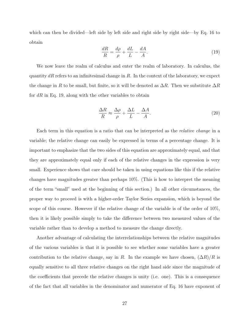
which can then be divided—left side by left side and right side by right side—by Eq. 16 to

obtaindR

R=

dρ

ρ+

dL

L− dA

A. (19)

We now leave the realm of calculus and enter the realm of laboratory. In calculus, the

quantity dR refers to an infinitesimal change in R. In the context of the laboratory, we expect

the change in R to be small, but finite, so it will be denoted as ∆R. Then we substitute ∆R

for dR in Eq. 19, along with the other variables to obtain

∆R

R≈ ∆ρ

ρ+

∆L

L− ∆A

A. (20)

Each term in this equation is a ratio that can be interpreted as the relative change in a

variable; the relative change can easily be expressed in terms of a percentage change. It is

important to emphasize that the two sides of this equation are approximately equal, and that

they are approximately equal only if each of the relative changes in the expression is very

small. Experience shows that care should be taken in using equations like this if the relative

changes have magnitudes greater than perhaps 10%. (This is how to interpret the meaning

of the term “small” used at the beginning of this section.) In all other circumstances, the

proper way to proceed is with a higher-order Taylor Series expansion, which is beyond the

scope of this course. However if the relative change of the variable is of the order of 10%,

then it is likely possible simply to take the difference between two measured values of the

variable rather than to develop a method to measure the change directly.

Another advantage of calculating the interrelationships between the relative magnitudes

of the various variables is that it is possible to see whether some variables have a greater

contribution to the relative change, say in R. In the example we have chosen, (∆R)/R is

equally sensitive to all three relative changes on the right hand side since the magnitude of

the coefficients that precede the relative changes is unity (i.e. one). This is a consequence

of the fact that all variables in the denominator and numerator of Eq. 16 have exponent of

27

unity. If the exponents had been something other than one, then some of the coefficients

before relative changes in Eq. 20 would be different than one as well. Thus the various terms

would have had different sensitivities.

In the expression for relative change in length, (∆L)/L, the variable L in the denomina-

tor refers to the current length of the strain gage grid after the strain is applied. We want to

express this as nominal strain, so we choose to normalize by the initial length instead; the dif-

ference in the ratio will be negligible as long as ∆L L. Therefore, we set εnom = (∆L)/L0.

It is straightforward to show by recourse to Hooke’s Law that (∆A)/A = −2ν(∆L)/L, ne-

glecting higher terms of (∆L)/L; Poisson’s ratio of the grid is denoted as ν. There results

after substitution into Eq. 20

∆R

R≈ ∆ρ

ρ+

∆L

L(1 + 2ν). (21)

Finally, dividing both sides of the equation by (∆L)/L, one obtains

G =(∆R)/R

(∆L)/L≈ (∆ρ)/ρ

(∆L)/L+ 1 + 2ν (22)

where G is the so-called gage factor of the strain gage. The first term on the right is called

the piezoresistivity which is a material property that relates the change in resistance to

strain. It is a constant for small strains and is tabulated.

The strain gage is sensitive to temperature changes because the variables in the expression

for the gage factor are temperature dependent and because, in general, the coefficients of

thermal expansion are different for the grid material, the matrix, and the object on which

the strain gage is applied. Temperature dependence can lead to substantial errors. A typical

method of dealing with it is discussed later.

An enlarged drawing of an actual strain gage is shown in Fig. 11. The gage length and

the gage width form the area over which the "average" strain is measured. The gage length

also provides the nominal length used in the definition of the gage factor. The gage length

28

GRID

WIDTH

OVERALL

PATTERN

LENGTH

MATRIX

LENGTH

OVERALL

PATTERN WIDTH

MATRIX WIDTH

GAGE

LENGTH

Figure 11: Drawing of Actual Strain Gage (Adapted from Catalog 500, Micro-MeasurementsDivision, Measurements Group, Inc., Raleigh, NC 27611)

ranges typically from less than 0.5 mm to 13 mm (0.016 in to 0.5 in). Strain gages are usually

manufactured with a nominal resistance of either 120 Ω or 350 Ω. A common grid material

is constantan (55% copper and 45% nickel) which has a gage factor of about G ≈ 2.0.

If a nominal strain level of εnom = 0.1% = 10−3 is measured with a 120 Ω strain gage

of gage factor G = 2.0, the resistance will change by ∆R = 0.24 so that (∆R)/R = 0.002.

The small magnitude of this ratio plays an important part in how the resistance changes are

measured.

Ideally, the resistance of a strain gage is a function of only the normal strain parallel to

its grid axis. In reality, however, the transverse strains affect the resistance. This effect can

be quantified but is often neglected.

If the stress state is uni-axial and in a known direction, a single strain gage will be

sufficient to define the strain state. However, to measure a general two-dimensional state

of strain at a point, three strain measurements must be made in different directions. The

29

R1

R4

R2

R3

vin

vout

Figure 12: Wheatstone Bridge

magnitudes and directions of the principal strains can then be calculated by means of a

Mohr’s circle analysis or, equivalently, by an eigenvalue/eigenvector analysis. To measure

the general state of strain, strain gages are made which incorporate a set of three grids which

are encapsulated at different orientations in the matrix. These “rosette” strain gages come in

two standard configurations: three grids mutually aligned 45 degrees apart and, three grids

mutually aligned 120 degrees apart.

Other strain gages are manufactured with two mutually perpendicular grids. These are

used to measure the magnitudes of principal strains when the their directions are known.

Alternatively, they can be used to measure the Poisson’s ratio of a material or to measure

the magnitude of the sum of the normal strains (an invariant with respect to direction) at a

point.

The very small changes of resistance characteristic to strain gages are difficult to measure

at a high resolution. For that reason, several special electrical circuits have been developed

30

for use with strain gages and other sensors. The Wheatstone Bridge electrical circuit is the

most common. A schematic diagram of the Wheatstone Bridge is shown in Fig. 12.

The circuit consists of four electrical resistors arranged as shown. The circuit is then

excited with an input voltage, vin. It can be shown from basic circuit analysis that the

corresponding output voltage, vout, is

vout = vin

R1R3 −R2R4

(R1 + R2)(R3 + R4)

. (23)

If the combination of resistances R1R3 − R2R4 = 0 then the bridge is said to be balanced

and vout = 0.

Strain gages are used as resistors in one or more arms of the bridge. From the discussion

of strain gages in Section 5.1, we note that the changes of electrical resistance is expected

to be very small during operation. Therefore, we expect any changes in vout to be very

small as well. Hence we adopt the strategy of calculating the total differential of Eq. 23 and

simplifying it in order to directly relate the changes of resistances with the change in vout.,

denoted as ∆vout. It can be shown (by neglecting second order terms) that

∆vout = vinR1R2

(R1 + R2)2

∆R1

R1− ∆R2

R2+

∆R3

R3− ∆R4

R4

(24)

where the ∆ notation indicates a small change in the value of the respective variables. This

form is particularly convenient because the (∆R)/R terms appear in the definition of the

gage factor of the strain gage in Eq. 22. Assuming that the nominal resistances of the bridge

are equal before any strain is applied, the expression reduces to

∆vout =vin

4

∆R1

R1− ∆R2

R2+

∆R3

R3− ∆R4

R4

. (25)

Now by identifying the nominal strain on strain gage #1 as ε1 = (∆L1)/L1 corresponding

to (∆R1)/R1 , etc., and by assuming that identical strain gages (both in terms of nominal

31

MM

#1

#3

#2

#4

Figure 13: Full Bridge Configuration

resistance as well as gage factor) are on each arm of the Wheatstone bridge, the expression

becomes

∆vout =Gvin

4[ε1 − ε2 + ε3 − ε4] . (26)

The Wheatstone Bridge circuit is often used in what is known as the quarter-bridge

configuration, where there is only one "active" strain gage (arm #1 of the bridge) and three

"dummy" resistors (resistors which do not change their value) in the other positions. The

strain experienced by the active gage is then related to the gage factor, input voltage and

change in output voltage as

ε1 =4

G

∆vout

vin. (27)

It is important to note that the Wheatstone Bridge is usually balanced under conditions

of zero applied strain. Therefore vout = 0 under conditions of zero strain so that ∆vout is

measured relative to zero.

By knowing the relationship between strains in an object, Eq. 26 can be further manipu-

lated. For example, Fig. 13 shows four strain gages mounted on a beam to make a transducer.

Strain gages #1 and # 3 are mounted on the top side of the beam and strain gages #2 and

#4 are mounted on the bottom side directly opposite the first two. Therefore, strain gages

#1 and #3 measure the strain on the top surface of the beam so that ε1 = ε3 = εtop. Like-

wise, strain gages #2 and #4 measure the strain on the bottom surface of the beam so that

ε1 = ε3 = εbottom. However for a beam under a constant moment, εtop = −εbottom. Thus,

32

Eq. 26 reduces to

εtop =1

G

∆vout

vin. (28)

There are two unexpected benefits to this configuration. Note that any temperature-related

resistance changes (they will be the same for each strain gage if they are bonded to the same

material in the same environment) in the strain gages will be exactly canceled out by terms

in Eq. 26 that have coefficients of opposite sign (such as ε1 and ε2). Likewise, the strains due

to an axial load (i.e one that would induce a strain of εtop = εbottom) are exactly canceled out.

The configuration in Fig. 13 is a full-bridge, temperature compensated transducer which

responds only to strains induced by a bending load.

Similarly, it would be simple to imagine a one-half bridge (two "active" strain gages and

two "dummy" resistors) configuration to measure the strains in a bar due to axial loading

while neglecting the strains due to a bending load. Again, the transducer is temperature

compensated.

To compensate for temperature changes in a Quarter-Bridge configuration (i.e. for a

single "active" strain gage in position #1) of the Wheatstone Bridge, it is common to apply

a "dummy" strain gage in position #2 to an identical type of material which is in the same

temperature environment but which is unstrained; in addition dummy resistors are placed

in arms #3 and #4 and maintained at equal temperatures. The change in resistance due to

temperature is then precisely canceled.

There are many data acquisition units on the market for the measurement of strains

with resistance strain gages. By connecting the strain gages in quarter-, half-, or full-bridge

configurations, specifying the type of configuration to the data acquisition device and entering

the strain gages’ gage factor, the level of strain is output directly in terms of microstrain

(µε). The strain resolution of the devices is usually 10−6 which is 1 µε.

33

6 Suggested Reading

There are many good texts and reference books on the subject of mechanical testing.Here is a list of just four of them, focusing on ductile metals.

• M. A. Meyers and K. K. Chawla, Mechanical Metallurgy, Prentice-Hall, 1984

• G. E. Dieter, Mechanical Metallurgy, McGraw-Hill, 1986

• N. E. Dowling, Mechanical Behavior of Materials, Prentice-Hall, 1993

• American Society for Testing and Materials (ASTM) develops and publishes standards

for the testing of materials.

34