introduction to modern canonical quantum general …arxiv:gr-qc/0110034v1 5 oct 2001 introduction to...

arX

iv:g

r-qc

/011

0034

v1 5

Oct

200

1

Introduction

to

Modern Canonical

Quantum General Relativity

T. Thiemann1

MPI f. Gravitationsphysik, Albert-Einstein-Institut,

Am Muhlenberg 1, 14476 Golm near Potsdam, Germany

Preprint AEI-2001-119

[email protected]

http://arXiv.org/abs/gr-qc/0110034v1

Abstract

This is an introduction to the by now fifteen years old research field of canonical quantum generalrelativity, sometimes called “loop quantum gravity”. The term “modern” in the title refers to the factthat the quantum theory is based on formulating classical general relativity as a theory of connectionsrather than metrics as compared to in original version due to Arnowitt, Deser and Misner.

Canonical quantum general relativity is an attempt to define a mathematically rigorous, non-perturbative, background independent theory of Lorentzian quantum gravity in four spacetime di-mensions in the continuum. As such it differs considerably from perturbative ansatze. It provides aunified theory of all interactions in the sense that all interactions transform under a common gaugegroup: The four-dimensional diffeomorphism group of the underlying differental manifold which ismaximally broken in perturbative approaches. The approach is minimal in that one simply ana-lyzes the logical consequences of combining the principles of general relativity with the principlesof quantum mechanics. As a consequence, no extra dimensions, no corresponding Kaluza-Kleincompactifications, no supersymmetry and its associated phenomenology – compatible spontaneousbreaking at low energies, seem to be necessary. On the other hand, no explanation for the particlecontent and the dimension of the universe is provided by the theory.

The requirement to preserve background independence has lead to new, fascinating mathematicalstructures which one does not see in perturbative approaches, e.g. a fundamental discreteness ofspacetime seems to be a prediction of the theory which is a first substantial evidence for a theory inwhich the gravitational field acts as a natural UV cut-off.

An effort has been made to provide a self-contained exposition at the appropriate level of rigourwhich at the same time is accessible to graduate students with only basic knowledge of generalrelativity and quantum field theory on Minkowski space. To be useful, not all facets of the field havebeen covered, however, guides to further reading and a detailed bibliography is included. This reportis submitted to the on-line journal “Living Reviews” and is thus subject to being updated on at leasta bi-annual basis.

Contents

Introduction 5Defining Quantum Gravity . . . . . . . . . . . . . . . . . . . . . . . . . . . . . . . . . 10

Why Quantum Gravity in the 21st Century ? . . . . . . . . . . . . . . . . . . 10The Role of Background Independence . . . . . . . . . . . . . . . . . . . . . . 14Approaches to Quantum Gravity . . . . . . . . . . . . . . . . . . . . . . . . . 15Motivation for Canonical Quantum General Relativity . . . . . . . . . . . . . 21

Notation and Conventions . . . . . . . . . . . . . . . . . . . . . . . . . . . . . . . . . 24

I Foundations 28I.1 Classical Hamiltonian Formulation of General Relativity and the Programme of Canon-

ical Quantization . . . . . . . . . . . . . . . . . . . . . . . . . . . . . . . . . . . . . . 29I.1.1 The ADM Formulation . . . . . . . . . . . . . . . . . . . . . . . . . . . . . . . 29I.1.2 The Programme of Canonical Quantization . . . . . . . . . . . . . . . . . . . . 42

I.1.2.1 The General Programme . . . . . . . . . . . . . . . . . . . . . . . . . 42I.1.2.2 Application to General Relativity in the ADM Formulation . . . . . 47

I.1.3 The New Canonical Variables of Ashtekar for General Relativity . . . . . . . . 49I.1.4 Functional Analytic Description of Classical Connection Dynamics . . . . . . . 62

I.2 Mathematical Foundations of Modern Canonical Quantum General Relativity . . . . 67I.2.1 The Space of Distributional Connections for Diffeomorphism Invariant Quan-

tum Gauge Theories . . . . . . . . . . . . . . . . . . . . . . . . . . . . . . . . 73I.2.1.1 The Label Set: Piecewise Analytic Paths . . . . . . . . . . . . . . . . 74I.2.1.2 The Topology: Tychonov Topology . . . . . . . . . . . . . . . . . . . 77I.2.1.3 Gauge Invariance: Distributional Gauge Transformations . . . . . . . 83

I.2.2 The C∗ Algebraic Viewpoint . . . . . . . . . . . . . . . . . . . . . . . . . . . . 90I.2.3 Regular Borel Measures on the Projective Limit: The Uniform Measure . . . . 97I.2.4 Functional Calculus on a Projective Limit . . . . . . . . . . . . . . . . . . . . 101I.2.5 Density and Support Properties of A,A/G with Respect to A,A/G . . . . . . 108I.2.6 Spin – Network Functions, Loop Representation, Gauge – and Diffeomorphism

Invariance of µ0 and Ergodicity . . . . . . . . . . . . . . . . . . . . . . . . . . 111I.3 Quantum Kinematics . . . . . . . . . . . . . . . . . . . . . . . . . . . . . . . . . . . . 119

I.3.1 Canonical Commutation – and Adjointness Relations . . . . . . . . . . . . . . 119I.3.1.1 Classical Lie Algebra of Functions and Vector Fields on A: Electric

Fluxes . . . . . . . . . . . . . . . . . . . . . . . . . . . . . . . . . . . 119I.3.1.2 Regularization of the Magnetic and Electric Flux Poisson Algebra . . 120I.3.1.3 Invariant Vector Fields on Gn . . . . . . . . . . . . . . . . . . . . . . 126I.3.1.4 Essential Self-Adjointness of Electric Flux Momentum Operators . . 129

2

I.3.1.5 Selection of the Uniform Measure by Adjointness Conditions . . . . . 130I.3.2 Implementation of the Gauss Constraint . . . . . . . . . . . . . . . . . . . . . 131

I.3.2.1 Derivation of the Gauss Constraint Operator . . . . . . . . . . . . . 131I.3.2.2 Complete Solution of the Gauss Constraint . . . . . . . . . . . . . . 132

I.3.3 Implementation of the Diffeomorphism Constraint . . . . . . . . . . . . . . . . 135I.3.3.1 Derivation of the Diffeomorphism Constraint Operator . . . . . . . . 135I.3.3.2 General Solution of the Diffeomorphism Constraint . . . . . . . . . . 136

I.4 Kinematical Geometrical Operators . . . . . . . . . . . . . . . . . . . . . . . . . . . . 141I.4.1 Derivation of the Area Operator . . . . . . . . . . . . . . . . . . . . . . . . . . 141I.4.2 Properties of the Area Operator . . . . . . . . . . . . . . . . . . . . . . . . . . 143I.4.3 Diffeomorphism Invariant Volume Operator . . . . . . . . . . . . . . . . . . . 147

II Current Research 149II.1 Quantum Dynamics . . . . . . . . . . . . . . . . . . . . . . . . . . . . . . . . . . . . . 150

II.1.1 The Wick Transform Proposal . . . . . . . . . . . . . . . . . . . . . . . . . . . 151II.1.1.1 The General Scheme . . . . . . . . . . . . . . . . . . . . . . . . . . . 152II.1.1.2 Wick Transform for Quantum Gravity . . . . . . . . . . . . . . . . . 155

II.1.2 Derivation of the Hamiltonian Constraint Operator . . . . . . . . . . . . . . . 156II.1.3 Mathematical Definition of the Hamiltonian Constraint Operator . . . . . . . 161

II.1.3.1 Concrete Implementation . . . . . . . . . . . . . . . . . . . . . . . . 161II.1.3.2 Operator Limits . . . . . . . . . . . . . . . . . . . . . . . . . . . . . 165II.1.3.3 Commutator Algebra . . . . . . . . . . . . . . . . . . . . . . . . . . . 166II.1.3.4 The Quantum Dirac Algebra . . . . . . . . . . . . . . . . . . . . . . 172

II.1.4 The Kernel of the Wheeler-DeWitt Constraint Operator . . . . . . . . . . . . 173II.1.5 Further Related Results . . . . . . . . . . . . . . . . . . . . . . . . . . . . . . 175

II.1.5.1 Generator of the Wick Transform . . . . . . . . . . . . . . . . . . . . 175II.1.5.2 Testing the New Regularization Technique by Models of Quantum

Gravity . . . . . . . . . . . . . . . . . . . . . . . . . . . . . . . . . . 176II.1.5.3 Quantum Poincare Algebra . . . . . . . . . . . . . . . . . . . . . . . 178

II.2 Extension to Standard Matter . . . . . . . . . . . . . . . . . . . . . . . . . . . . . . . 181II.2.1 Kinematical Hilbert Spaces for Diffeomorphism Invariant Theories of Fermionic

and Higgs Fields . . . . . . . . . . . . . . . . . . . . . . . . . . . . . . . . . . 181II.2.1.1 Fermionic Sector . . . . . . . . . . . . . . . . . . . . . . . . . . . . . 181II.2.1.2 Higgs Sector . . . . . . . . . . . . . . . . . . . . . . . . . . . . . . . 184II.2.1.3 Gauge and Diffeomorphism Invariant Subspace . . . . . . . . . . . . 186

II.2.2 Quantization of Matter Hamiltonian Constraints . . . . . . . . . . . . . . . . . 187II.2.2.1 Quantization of Einstein-Yang-Mills-Theory . . . . . . . . . . . . . . 188II.2.2.2 A General Quantization Scheme . . . . . . . . . . . . . . . . . . . . . 190

II.3 Semiclassical Analysis . . . . . . . . . . . . . . . . . . . . . . . . . . . . . . . . . . . 192II.3.1 Weaves . . . . . . . . . . . . . . . . . . . . . . . . . . . . . . . . . . . . . . . . 193II.3.2 Coherent States . . . . . . . . . . . . . . . . . . . . . . . . . . . . . . . . . . . 195

II.3.2.1 Semiclassical States and Coherent States . . . . . . . . . . . . . . . . 196II.3.2.2 Construction Principle: Complexifier Method and Heat Kernels . . . 198II.3.2.3 Coherent States for Canonical Quantum General Relativity . . . . . 200II.3.2.4 The Infinite Tensor Product Extension . . . . . . . . . . . . . . . . . 206

II.3.3 Photon Fock States on A . . . . . . . . . . . . . . . . . . . . . . . . . . . . . . 211

3

II.3.4 Applications . . . . . . . . . . . . . . . . . . . . . . . . . . . . . . . . . . . . . 214II.4 Further Research Directions . . . . . . . . . . . . . . . . . . . . . . . . . . . . . . . . 216

II.4.1 Spin Foam Models . . . . . . . . . . . . . . . . . . . . . . . . . . . . . . . . . 216II.4.2 Quantum Black Hole Physics . . . . . . . . . . . . . . . . . . . . . . . . . . . 224II.4.3 Connections Between Canonical Quantum General Relativity and String – (M)

Theory . . . . . . . . . . . . . . . . . . . . . . . . . . . . . . . . . . . . . . . . 231II.5 Selection of Open Research Problems . . . . . . . . . . . . . . . . . . . . . . . . . . . 233

III Mathematical Tools 236III.1 The Dirac Algorithm for Field Theories with Constraints . . . . . . . . . . . . . . . . 237III.2 Elements of Fibre Bundle Theory . . . . . . . . . . . . . . . . . . . . . . . . . . . . . 244III.3 Tools from General Topology . . . . . . . . . . . . . . . . . . . . . . . . . . . . . . . 253III.4 Elementary Introduction to Gel’fand Theory for Abelean C∗ Algebras . . . . . . . . . 259III.5 Tools from Measure Theory . . . . . . . . . . . . . . . . . . . . . . . . . . . . . . . . 269III.6 Spectral Theorem and GNS-Construction . . . . . . . . . . . . . . . . . . . . . . . . . 276III.7 Introduction to Refined Algebraic Quantization (RAQ) . . . . . . . . . . . . . . . . . 280

4

Introduction

This report tries to give a status overview of the field of modern canonical quantum general relativity,sometimes called “loop quantum gravity”. The term “modern” accounts for the fact that this is a“connection dynamics” formulation of Einstein’s theory, rather than the original “geometrodynamics”formulation due to Arnowitt, Deser and Misner. As this is an article submitted to the on-line journal“Living Reviews, the report will be updated on an at least bi-annual basis.

The field of modern canonical quantum general relativity was born in 1986 and since then anorder of 500 research papers closely related to the subject have been published. Pivotal structuresof the theory are scattered over an order of 100 research papers, reports, proceedings and books,issues which were believed to be essential initially turned out to be negligible later on and viceversa. These facts make it hard for the beginner to go quickly to the frontier of original research.The present report aims at giving beginners a guideline, a kind of geodesic through the literaturesuggesting in which order to read a minimal number of papers in order to understand the founda-tions. The report should be accessible to students at the graduate level (say European studentsin their sixth or seventh semester) with only basic prior knowledge of general relativity and quan-tum field theory on Minkowski space. However, the target audience does not consist of the lighthearted readers who wish to get just some rough idea of what the field is all about, those readersare advised to study the excellent review articles [1, 2, 3]. Rather, we typically have in mind theserious student who wants to gain thorough understanding of the foundations and to pass quicklyto the frontier of active research. As financial support over an extended period of time is a seriousissue for almost all graduate students in the world, time is pressing and it is important that onedoes not waste too much time in learning the basics. We have therefore decided to select only aminimal amount of material, just enough in order to reach a firm understanding of the foundations,which on the other hand is presented in great detail so that one does not have to read much besidesthis report for this purpose. Since some of the mathematics that is needed maybe unfamiliar to theyounger students we have also included a large mathematical “appendix” that serves to fill in someof the necessary background. Remembering too freshly still our own experience how annoying andtime consuming it can be to collect papers, to compare and streamline notations, to adapt numer-ical coefficient conventions etc. this should also help to avoid unnecessary confusions and time delays.

The number of people working in the field of canonical quantum general relativity is of the or-der of 102 (including students and post-docs) which is unfortunately quite small, when compared,for instance, with the size of the string theory community (of the order 103) and it is one of the aimsof this report to attract more young researchers to dive into this alternative, fascinating researchsubject. Here is a, to the best knowledge of the author, complete list of locations where researchin canonical quantum general relativity (and related) is, at least partly, currently performed andfunded together with the names of main contact persons in alphabetical order and their main currentresearch directions. The locations are listed alphabetically by continent and within one continentgeographically by country from north to south (p=permanent position, n=non-permanent position,we only list post-docs among the non-permanent staff):

A) Central America

1. Universidad Autonoma Metropolitana Itztapalapa, Mexico City, Mexico

Hugo Morales-Tecotl (p): semiclassical quantum gravity

2. Universidad Nacionale Autonoma de Mexico, Mexico City, Mexico

5

Alexandro Corichi (p): semiclassical quantum gravity, isolated horizon quantum blackholes;Michael Ryan (p) : mini(midi)superspace models;Jose-Antonio Zapata (p) : semiclassical quantum gravity, spin foams

B) North America

3. University of Alberta, Edmonton, Canada

Stephen Fairhurst (n): isolated horizon quantum black holes;Viquar Husain (p): mini(midi)superspace and integrable models;Don Page (p): mini(midi)superspace models

4. Perimeter Institute for Theoretical Physics and University of Waterloo, Waterloo, On-tario, Canada

Olaf Dreyer (n): isolated horizon quantum black holes;Fotini Markopoulou (p): causal spin foams, renormalization;Lee Smolin (p): connections between loop quantum gravity and string theory, causalquantum dynamics, spin foam models;O. Winkler (n): semi-classical quantum gravity

5. Syracuse University, Syracuse, NY, USA

Donald Marolf (p): refined algebraic quantization, general relativistic aspects of stringtheory

6. Center for Gravitational Physics and Geometry, The Pennsylvania State University atUniversity Park, PA, USA

Abhay Ashtekar (p): isolated horizon quantum black holes, semi-classical quantum grav-ity;Martin Bojowald (n): mini(midi)superspace models, quantum dynamics;Amit Ghosh (n): isolated horizon black holes;Roger Penrose1 (p): twistor theory, fundamental issues;Alexandro Perez (n): spin foam models

7. University of Utah, Salt Lake City, UT, USA

Christopher Beetle (n): covariant formulation;Karel Kuchar (p): mini – and midisuperspace models, covariant formulation

8. University of Maryland, College Park, MD, USA

Ted Jacobson (p): classical actions, (quantum) black hole physics

9. Kansas State Unviversity, Kansas City, KS, USA

Louis Crane (p): state sum models, spin foam models;David Yetter(p): state sum models, spin foam models

10. Utah State University, Logan, UT, USA

Charles Torre (p): mini(midi)superspace models, fundamental issues

11. University of California, Riverside, CA, USA

John Baez (p): isolated horizon quantum black holes, spin foam models

1Distinguished Visiting Professor from the University of Oxford, Oxford, UK

6

12. University of California and Institute of Theoretical Physics, Santa Barbara, CA, USA

Jim Hartle (p): connection between consistent histories – and canonical approach;Kirill Krasnov (n) : isolated horizon quantum black holes, spin foam models, aspects ofstring theory

13. University of Mississippi, Oxford, MS, USA

Luca Bombelli (p): semiclassical quantum gravity

14. Lousiana State University, Baton Rouge, LA, USA

Jorge Pullin (p): quantum dynamics, Dirac observables, semiclassical quantum gravity

C) South America

15. Universidad de la Republica, Montevideo, Uruguay

Rodolfo Gambini (p): quantum dynamics, Dirac observables;Jorge Griego (p): quantum dynamics;Michael Reisenberger (p): dynamical lattice formulations, spin foam models

16. Centro de Estudios Cientificos, Valdivia, Chile

Claudio Teitelboim: mini(midi)superspace models, quantization of gauge systems;Andres Gomberoff (p): refined algebraic quantization, general relativistic aspects of stringtheory

D) Asia

17. Raman Research Institute, Bangalore, India

Joseph Samuel (p): classical formulation;Madhavan Varadarajan (p): semiclassical quantum gravity

E) Europe

18. The Niels Bohr Institute, Copenhagen, Denmark

Jan Ambjorn (p): path integral formulation (dynamical triangulations);Matthias Arnsdorf (n): semiclassical quantum gravity, connections with string theory

19. University of Nottingham, Nottingham, UK

John Barrett (p): spin foam models, state sum models;Jorma Louko (p): mini(midi)superspace models, general relativistic aspects of string the-ory

20. Albert – Einstein – Institut, Golm near Potsdam, Germany

Hermann Nicolai (p): supergravity, superstring theory, connections between canonicalquantum gravity and M – Theory;Thomas Thiemann (p): quantum dynamics, semi-classical analysis

21. University of Warsaw, Warsaw, Poland

Jurek Lewandowski (p): isolated horizon quantum black holes, semi-classical quantumgravity

22. Utrecht University and Spinoza Institute, Utrecht, The Netherlands

Gerhard ’t Hooft (p): quantum black hole physics, fundamental issues;Renate Loll (p): quantum geometry, path integral formulation (dynamical triangulations)

7

23. Cambridge University, Cambridge, UK

Ruth Williams (p): spin foam models, state sum models

24. Imperial College, London, UK

Chris Isham (p): fundamental issues (topos theory)

25. Universite Libre de Bruxelles, Bruxelles, Belgium

Marc Henneaux (p): BRST analysis, quantization of gauge systems, general relativisticaspects of supergravity and string theory

26. Ecole Normale Superieure, Paris, France

Bernard Julia (p): canonical quantization of supergravity theories, Noether charges

27. Universitat Wien, Wien, Austria

Peter Aichelburg (p): general relativistic aspects of supergravity and string theory

28. Universitat Bern, Bern, Switzerland

Peter Hajicek (p): midi(mini)superspace models

29. Ecole Normale Superieur, Lyon, France

Laurent Freidel (p) : spin foam models

30. Universita di Torino, Torino, Italy

Jeanette Nelson (p): mini(midi)superspace models, Regge calculus

31. Universita di Parma, Parma, Italy

Roberto de Pietri (n) : quantum dynamics, spin foam models

32. Universite de Marseille, Luminy, France

Carlo Rovelli (p): quantum dynamics, Dirac observables, spin foam models

33. Instituto de Matematicas y Fisica Fundamental, Madrid, Spain

Guillermo Mena-Maguan (p): mini(midi)superspace models, Euclidean versus Lorentzianformulation

34. Universidad Europea, Madrid, Spain

Fernando Barbero (p): classical actions

35. Instituto Superior Tecnico, Lisboa, Portugal

Jose Mourao (p): mathematical framework

36. Universidad do Algarve, Faro, Portugal

Nenad Manojlovic (p): mini(midi)superspaces, integrable models

All these places are definitely worthwhile applying to for graduate studies or post-doc positions.Notice that we have listed only those researchers that are at least partly involved or interested inquantum general relativity research and only those aspects of their work that touch on quantumgravity. For instance, the Albert – Einstein – Institute is currently the largest (by number of mem-bers and budget) institute in the world that focusses on gravitational physics, consisting of altogetherfour divisions: Quantum Gravity and Unified Theories with focus on M – Theory (director: HermannNicolai), Astrophysics (director: Bernard Schutz), Mathematical General Relativity (director: Ger-hard Huisken), Gravitational Wave Detection (director: Karsten Danzmann). Institutes of similarsizes are the Center for Gravitational Physics and Geometry, the Perimeter Institute for TheoreticalPhysics and the Institute for Theoretical Physics at Santa Barbara. Unfortunately the University of

8

Pittsburgh, Pittsburgh, PA, USA (Ted Newman (p): null surface formulation, fundamental issues)no longer appears in the above list since quantum gravitational research is no longer funded there.

This report is organized as follows :

Before diving into the subject, the next subsection motivates the search for a quantum theory ofgravity, points out what the essential problems are that one has to deal with, lists the possible ap-proaches and their respective strengths and weaknesses and finally motivates our choice to studycanonical quantum general relativity. We also list our notation and conventions.

We then approach the main text of the report which is subdivided into three parts:

The first part contains the foundations of the theory, that is, results which are physically andmathematically robust. Thus we will study in detail a) the classical canonical formulation of generalrelativity in terms of connection variables, b) the general programme of canonical quantization, c)the application of this programme to general relativity in terms of connections and the resultingHilbert space structures, d) the proof that the Hilbert space found implements the correct quantumkinematics (that is, it represents the correct commutation relations and supports the kinematicalconstraints of the theory) and finally e) the kinematical geometrical operators which measure forinstance areas of (coordinate) surfaces. We also sketch how spectral properties of these kinematicaloperators extend to their physical (dynamical) counterparts in the presence of matter.

The second part discusses the main, current research directions within canonical quantum generalrelativity and describes their respective status. These results are less robust and still, at leastpartially, in flow. Thus we outline in detail a) the implementation of the quantum dynamics orQuantum Einstein Equantions (also known by “Wheeler – DeWitt Equation”), b) the couplingof standard quantum matter, c) the semiclassical analysis necessary in order to verify whether thetheory constructed is indeed a quantization of general relativity, d) the path integral formulationof the theory (also called spin foam formulation), e) quantum black hole physics and finally f) thepossible links between string theory and canonical quantum general relativity. This part closes witha section in which we list a selected number of open and fascinating research problems.

Finally, in the third part we provide some mainly mathematical background material. Thus wegive elementary but fairly extensive introductions to elements of a) the Dirac algorithm for dealingwith theories with constraints, b) the theory of fibre bundles, c) general topology, d) Gel’fand the-ory for Abelean C∗−algebras, e) measure theory, f) the GNS construction and g) refined algebraicquantization (RAQ).

Acknowledgements

My thanks go to Theresa Velden, for a long time managing director of the on-line journal “Liv-ing Reviews”, for continuously encouraging me to finally finish this review.

9

Defining Quantum Gravity

In the first subsection of this section we explain why the problem of quantum gravity cannot beignored in nowadays physics, even though the available accelerator energies lie way beyond the Planckscale. Then we define what a quantum theory of gravity and all interactions is widely expected toachieve and point out the two main directions of research divided into the perturbative and non-perturbative approaches. In the third subsection we describe these approaches in more detail andfinally in the fourth motivate our choice to do canonical quantum general relativity as opposed toother approaches.

Why Quantum Gravity in the 21st Century ?

It is often argued that quantum gravity is not relevant for the physics of this century because in ourmost powerful accelerator, the LHC to be working in 2005, we obtain energies of the order of a few103 GeV while the energy scale at which quantum gravity is believed to become important is thePlanck energy of 1019 GeV. While that is true, it is false that nature does not equip us with particlesof energies much beyond the TeV scale, there are astrophysical particles with energy of a fist strokeand the next generation of particle microscopes is therefore not going to be built on the surface ofEarth any more but in its orbit. Moreover, as we will describe in this report in more detail, evenwith TeV energy scales it might be possible to see quantum gravity effects in the close future.

But even apart from these purely experimental considerations, there are good theoretical reasonsfor studying quantum gravity. To see why, let us summarize our current understanding of the fun-damental interactions :Ashamingly, the only quantum fields that we fully understand to date in four dimensions are freequantum fields on four-dimensional Minkowski space. Formulated more provocatively:

In four dimensions we only understand an (infinite) collection of uncoupled harmonicoscillators on Minkowski space !

In order to leave the domain of these rather trivial and unphysical quantum field theories, physicistshave developed two techniques : perturbation theory and quantum field theory on curved back-grounds. This means the following :With respect to accelerator experiments, the most important processes are scattering amplitudesbetween particles. One can formally write down a unitary operator that accounts for the scatter-ing interaction between particles and which maps between the well-understood free quantum fieldHilbert spaces in the far past and future. Famously, by Haags theorem [4], whenver that operatoris really unitary, there is no interaction and if it is not unitary, then it is ill-defined. In fact, onecan only define the operator perturbatively by writing down the formal power expansion in terms ofthe generator of the would-be unitary transformation between the free quantum field theory Hilbertspaces. The resulting series is divergent order by order but if the theory is “renormalizable” thenone can make these orders artificially finite by a regularization and renormalization procedure with,however, no control on convergence of the resulting series. Despite these drawbacks, this recipe hasworked very well so far, at least for the electroweak interaction.

Until now, all we have said applies only to free (or perturbatively interacting) quantum fields onMinkowski spacetime for which the so-called Wightman axioms [4] can be verified. Let us summarizethem for the case of a scalar field in (D + 1)−dimensional Minkowski space:

10

W1 RepresentationThere exists a unitary and continuous representation U : P → B(H) of the Poincare groupP on a Hilbert space H.

W2 Spectral ConditionThe momentum operators P µ have spectrum in the forward lightcone:ηµνP

µP ν ≤ 0; P 0 ≥ 0.

W3 VacuumThere is a unique Poincare invariant vacuum state U(p)Ω = Ω for all p ∈ P .

W4 CovarianceConsider the smeared field operator valued tempered distributions φ(f) =

∫RD+1 dD+1xφ(x)f(x)

where f ∈ S(RD+1) is a test function of rapid decrease. Then finite linear combinations of theform φ(f1)..φ(fN)Ω lie dense in H (that is, Ω is a cyclic vector) and U(p)φ(f)U(p)−1 = φ(f p)for any p ∈ P .

W5 Locality (Causality)Suppose that the supports (the set of points where a function is different from zero) of f, f ′ arespacelike separated (that is, the points of their supports cannot be connected by a non-spacelikecurve) then φ(f), φ(f ′) = 0.

The most important objects in this list are those that are highlighted in bold face letters: The fixed,non-dynamical Minkowski background metric η with its well-defined causal structure, its Poincaresymmetry group P , the associated representation U(p) of its elements, the invariant vacuum state Ωand finally the fixed, non-dynamical topological, differentiable manifold RD+1. Thus the Wightmanaxioms assume the existence of a non-dynamical, Minkowski background metric which implies thatwe have a preferred notion of causality (or locality) and its symmetry group, the Poincare group fromwhich one builds the usual Fock Hilbert spaces of the free fields. We see that the whole structure ofthe theory is heavily based on the existence of these objects which come with a fixed, non-dynamicalbackground metric on a fixed, non-dynamical topological and differentiable manifold.

For a general background spacetime, things are already under much less control: We still havea notion of causality (locality) but generically no symmetry group any longer and thus there is noobvious generalization of the Wightman axioms and no natural perturbative Fock Hilbert space anylonger. These obstacles can partly be overcome by the methods of algebraic quantum field theory[5] and the so-called microlocal analysis [6] (in which the locality axiom is taken care of pointwiserather than globally) which recently have also been employed to develop perturbation theory on ar-bitrary background spacetimes [7] by invoking the mathematically more rigorous implementation ofthe renormalization programme developed by Epstein and Glaser in which no divergent expressionsever appear at least order by order (see, e.g., [8]).

However, the whole framework of ordinary quantum field theory breaks down once we make thegravitational field (and the differentiable manifold) dynamical, once there is no background metricany longer !

Combining these issues, one can say that we have a working understanding of scattering processesbetween elementary particles in arbitrary spacetimes as long as the backreaction of matter on geom-etry can be neglected and that the coupling constant between non-gravitational interactions is small

11

enough (with QCD being an important exception) since then the classical Einstein equation, whichsays that curvature of geometry is proportional to the stress energy of matter, can be approximatelysolved by neglecting matter altogether. Thus, for this set-up, it seems fully sufficient to have only aclassical theory of general relativity and perturbative quantum field theory on curved spacetimes.

From a fundamental point of view, however, this state of affairs is unsatisfactory for many reasonsamong which we have the following:

i) Classical Geometry – Quantum Matter InconsistencyAt a fundamental level, the backreaction of matter on geometry cannot be neglected. Namely,geometry couples to matter through Einstein’s equations

Rµν − 1

2R · gµν = κTµν[g]

and since matter undelies the rules of quantum mechanics, the right hand side of this equation,the stress-energy tensor Tµν [g], becomes an operator. One has tried to keep geometry classicalwhile matter is quantum mechanical by replacing Tµν [g] by the Minkowski vacuum expectation

value < Tµν [η] > but the solution of this equation will give g 6= η which one then has to feedback into the definition of the vacuum expectation value etc. The resulting iteration does notconverge in general. Thus, such a procedure is also inconsistent whence we must quantize thegravitational field as well. This leads to the Quantum Einstein Equations

Rµν − 1

2R · gµν = κTµν[g]

Of course, this equation is only formal at this point and must be embedded in an appropriateHilbert space context.

ii) Inherent Classical Geometry InconsistencyEven without quantum theory at all Einstein’s field equations predict spacetime singularities(black holes, big bang singularities etc.) at which the equations become meaningless. In a trulyfundamental theory, there is no room for such breakdowns and it is suspected by many thatthe theory cures itself upon quantization in analogy to the Hydrogenium atom whose stabilityis classically a miracle (the electron should fall into the nucleus after a finite time lapse due toemission of Bremsstrahlung) but is easily explained by quantum theory.

iii) Inherent Quantum Matter InconsistencyAs outlined above, perturbative quantum field theory on curved spacetimes is itself also ill-defined due to its UV (short distance) singularities which can be cured only with an ad hocrecipe order by order which lacks a fundamental explanation, moreover, the perturbation seriesis presumably divergent. Besides that, the usually infinite vacuum energies being usuallyneglected in such a procedure contribute to the cosmological constant and should have a largegravitational backreaction effect. That such energy subtractions are quite significant is maybebest demonstrated by the Casimir effect. Now, since general relativity possesses a fundamentallength scale, the Planck length, it has been argued ever since that gravitation plus mattershould give a finite quantum theory since gravitation provides the necessary, built-in, shortdistance cut-off.

iv) Perturbative Quantum Geometry InconsistencyGiven the fact that perturbation theory works reasonably well if the coupling constant is small

12

for the non-gravitational interactions on a background metric it is natural to try whetherthe methods of quantum field theory on curved spacetime work as well for the gravitationalfield. Roughly, the procedure is to write the dynamical metric tensor as g = η + h where ηis the Minkowski metric and h is the deviation of g from it. One arrives at a formal, infiniteseries with finite radius of convergence which becomes meaningless if the fluctuations are large.Although the naive power counting argument implies that general relativity so defined is a non-renormalizable theory it was hoped that due to cancellations of divergencies the perturbationtheory could be actually finite. However, that this hope was unjustified was shown in [9] wherecalculations demonstrated the appearance of divergencies at the two-loop-level, which suggeststhat at every order of perturbation theory one must introduce new coupling constants whichthe classical theory did not know about and one loses predictability.

It is well-known that the (locally) supersymmetric extension of a given non-supersymmetricfield theory usually improves the ultra-violet convergence of the resulting theory as compared tothe original one due to fermionic cancellations [10]. It was therefore natural to hope that quan-tized supergravity might be finite. However, in [11] a serious argument against the expectedcancellation of perturbative divergences was raised and recently even the again popular (due toits M-Theory context) most complicated 11D “last hope” supergravity theory was shown notto have the magical cancellation property [12].

Summarizing, although a definite proof is still missing up to date (mainly due to the highlycomplicated algebraic structure of the Feynman rules for quantized supergravity) it is todaywidely believed that perturbative quantum field theory approaches to quantum gravity aremeaningless.

The upshot of these considerations is that our understanding of quantum field theory and thereforefundamental physics is quite limited unless one quantizes the gravitational field as well. Being verysharply critical one could say:

The current situation in fundamental physics can be compared with the one at theend of the nineteenth century: While one had a successful theory of electromagnetism,one could not explain the stability of atoms. One did not need to worry about thisfrom a practical point of view since atomic length scales could not be resolved at thattime but from a fundamental point of view, Maxwell’s theory was incomplete. The dis-covery of the mechanism for this stability, quantum mechanics, revolutionized not onlyphysics. Still today we have no thorough understanding for the stability of nature (anexperiment that everybody can repeat by looking out of the window) and it is similarlyexpected that the more complete theory of quantum gravity will radically change ourview of the world. That is, considering the metric as a quantum operator will bring usbeyond standard model physics even without the discovery of new forces, particles orextra dimensions.

13

The Role of Background Independence

The twentieth century has dramatically changed our understanding of nature : It revealed thatphysics is based on two profound principles : quantum mechanics and general relativity. Bothprinciples revolutionize two pivotal structures of Newtonian physics : First, the determinism ofNewton’s equations of motion evaporates at a fundamental level, rather dynamics is reigned byprobabilities underlying the Heisenberg uncertainty obstruction. Secondly, the notion of absolutetime and space has to be corrected, space and time and distances between points of the spacetimemanifold, that is, the metric, become themselves dynamical, geometry it is no longer just an observer.The usual Minkowski metric ceases to be a distinguished, externally prescribed, background structure.Rather, the laws of physics are background independent, mathematically expressed by the classicalEinstein equations which are generally (or four-diffeomorphism) covariant. As we have argued, itis this new element of background independence brought in with Einstein’s theory of gravity whichcompletely changes our present understanding of quantum field theory.

A satisfactory physical theory must combine both of these fundamental principles, quantum me-chanics and general relativity, in a consistent way and will be called “Quantum Gravity”. However,the quantization of the gravitational field has turned out to be one of the most challenging unsolvedproblems in theoretical and mathematical physics. Although numerous proposals towards a quanti-zation have been made since the birth of general relativity and quantum theory, none of them canbe called successful so far. This is in sharp contrast to what we see with respect to the other threeinteractions whose description has culminated in the so-called standard model of matter, in partic-ular, the spectacular success of perturbative quantum electrodynamics whose theoretical predictionscould be verified to all digits within the experimental error bars until today.

Today we do not have a theory of quantum gravity, what we have is :1) The Standard Model, a quantum theory of the non-gravitational interactions (electromagnetic,weak and strong) or matter which, however, completely ignores general relativity.2) Classical General Relativity or geometry, which is a background independent theory of all inter-actions but completely ignores quantum mechanics.

What is so special about the gravitational force that it persists its quantization for about seventyyears already ? As outlined in the previous subsection, the answer is simply that today we onlyknow how to do Quantum Field Theory (QFT) on fixed background metrics. The whole formalism ofordinary QFT heavily relies on this background structure and collapses to nothing when it is missing.It is already much more difficult to formulate a QFT on a non-Minkowski (curved) background butit seems to become a completely hopeless task when the metric is a dynamical, even fluctuatingquantum field itself. This underlines once more the source of our current problem of quantizinggravity : We have to learn how to do QFT on a differential manifold (or something even morerudimentary, not even relying on a fixed topological, differentiable manifold) rather than a spacetime.

In order to proceed, today a high energy physicist has the choice between the following two,extreme approaches :Either the particle physicist’s, who prefers to take over the well-established mathematical machineryfrom QFT on a background at the price of dropping background independence altogether to beginwith and then tries to find the true background independent theory by summing the perturbationseries (summing over all possible backgrounds). Or the quantum geometer’s, who believes thatbackground independence lies at the heart of the solution to the problem and pays the price tohave to invent mathematical tools that go beyond the framework of ordinary QFT right from thebeginning. Both approaches try to unravel the truly deep features that are unique to Einstein’stheory associated with background independence from different ends.

14

The particle physicist’s language is perturbation theory, that is, one writes the quantum metricoperator as a sum consisting of a background piece and a perturbation piece around it, the graviton,thus obtaining a graviton QFT on a Minkowski background. We see that perturbation theory, byits very definition, breaks background independence and diffeomorphism invariance at every finiteorder of perturbation theory. Thus one can restore background independence only by summing upthe entire perturbation series which is of course not easy. Not surprisingly, as already mentioned,applying this programme to Einstein’s theory itself results in a mathematical desaster, a so-callednon-renormalizable theory without any predictive power. In order to employ perturbation theory, itseems that one has to go to string theory which, however, requires the introduction of new additionalstructures that Einstein’s classical theory did not know about: supersymmetry, extra dimensionsand an infinite tower of new and very heavy particles next to the graviton. This is a fascinating butextremely drastic modification of general relativity and one must be careful not to be in conflict withphenomenology as superparticles, Kaluza Klein modes from the dimensional reduction and thoseheavy particles have not been observed until today. On the other hand, string theory has a goodchance to be a unified theory of the perturbative aspects of all interactions in the sense that allinteractions follow from a common object, the string, thereby explaining the particle content of theworld.

The quantum geometer’s language is a non-perturbative one, keeping background independenceas a guiding principle at every stage of the construction of the theory, resulting in mathematicalstructures drastically different form the ones of ordinary QFT on a background metric. One takesEinstein’s theory absolutely seriously, uses only the principles of general relativity and quantummechanics and lets the theory build itself, driven by mathematical consistency. Any theory meetingthese standards will be called Quantum General Relativity (QGR). Since QGR does not modify thematter content of the known interactions, QGR is therefore not in conflict with phenomenology butalso it cannot explain the particle content so far. However, it tries to unify all interactions in adifferent sense: all interactions must transform under a common gauge group, the four-dimensionaldiffeomorphism group which on the other hand is mlmost completely broken in perturbative ap-proaches.

Let us remark that even without specifying further details, any QGR theory is a promisingcandidate for a theory that is free from two divergences of the so-called perturbation series of Feynmandiagrammes common to all perturbative QFT’s on a background metric: (1) Each term in the seriesdiverges due to the ultraviolet (UV) divergences of the theory which one can cure for renormalizabletheories, such as string theory, through so-called renormalization techniques and (2) the series of theserenormalized, finite terms diverges, one says the theory is not finite. The first, UV, problem has achance to be absent in a background independent theory for a simple but profound reason: In order toto say that a momentum becomes large one must refer to a background metric with respect to whichit is measured, but there simply is no background metric in the theory. The second, convergence,problem of the series might be void as well since there are simply no Feynman diagrammes ! Thus,the mere existence of a consistent background independent quantum gravity theory could imply afinite quantum theory of all interactions.

Approaches to Quantum Gravity

The aim of the previous subsection was to convince the reader that background independence is,maybe, The Key Feature of quantum gravity to be dealt with. No matter how one deals with thisissue, whether one starts from a perturbative (= background dependent) or from a non-perturbative(= background independent) platform, one has to invent something drastically new in order to

15

quantize the gravitational field. We will now explain these approaches in more detail, listed indecreasing numbers of researchers working in the respective fields.

1) Perturbative Approach : String TheoryThe only known consistent perturbative approach to quantum gravity is string theory whichhas good chances to be a theory that unifies all interactions. String Theory [13] is not afield theory in the ordinary sense of the word. Originally, it was a two-dimensional fieldtheory of world-sheets embedded into a fixed, D-dimensional pseudo-Riemannian manifold(M, g) of Lorentzian signature which is to be thought of as the spacetime of the physical world.The Lagrangean of the theory is a kind of non-linear σ−model Lagrangean for the associatedembedding variables X (and their supersymmetric partners in case of the superstring). If oneperturbes g(X) = η + h(X) as above and keeps only the lowest order in X one obtains afree field theory in two dimensions which, however, is consistent only when D = 26 (bosonicstring) or D = 10 (superstring) respectively. Strings propagating in those dimensions are calledcritical strings, non-critiical strings exist but have so far not played a significant role due tophenomenological reasons. Remarkably, the mass spectrum of the particle-like excitations ofthe closed worldsheet theory contain a massless spin-two particle which one interprets as thegraviton. Until recently, the superstring was favoured since only there it was believed to bepossible to get rid off an unstable tachyonic vaccum state by the GSO projection. However,one recently also tries to construct stable bosonic string theories [14].

Moreover, if one incorporates the higher order terms h(X) of the string action, sufficient forone loop corrections, into the associated path integral one finds a consistent quantum theoryup to one loop only if the background metric satisfies the Einstein equations. These are themost powerful outcomes of the theory : although one started out with a fixed backgroundmetric, the background is not arbitrary but has to satisfy the Einstein equations up to higherloop corrections indicating that the one-loop effective action for the low energy quantum fieldtheory in those D dimensions is Einstein’s theory plus corrections. Finally, at least the typeII superstring theories are are one-loop and, possibly, to all orders, finite. String theoriststherefore argue to have found candidates for a consistent theory of quantum gravity with theadditional advantage that they do not contain any free parameters (like those of the standardmodel) except for the string tension.

These facts are very impressive, however, some cautionary remarks are appropriate:

– Vacuum DegeneracyDimension D+1 = 10, 26 is not the dimension of everyday physics so that one has to arguethat the extra D − 3 dimensions are “tiny” in the Kaluza-Klein sense although nobodyknows the mechanism responsible for this “spontaneous compactification”. According to[15] there exists an order of 104 consistent, distinct Calabi-Yau compactifications (othercompactifications such as toroidal ones seem to be inconsistent with phenomenology)each of which has an order of 102 free, continuous parameters (moduli) like the vacuumexpectation value of the Higgs field in the standard model. For each compactification ofeach of the five string theories in D = 10 dimensions and for each choice of the moduli oneobtains a distinct low energy effective theory. This is clearly not what one expects from atheory that aims to unify all the interactions, the 18 (or more for massive neutrinos) free,continuous parameters of the standard model have been replaced by 102 continuous plusat least 104 discrete ones.

This vacuum degeneracy problem is not cured by the M-Theory interpretation of string

16

theory but it is conceptually simplified if certain conjectures are indeed correct : Stringtheorists believe (bearing on an impressively huge number of successful checks) that so-called T (or target space) and S (or strong – weak coupling) duality transformationsbetween all these string theories exist which suggest that we do not have 104 unrelated102-dimensional moduli spaces but that rather these 102-dimensional manifolds intersect insingular, lower dimensional submanifolds corresponding to certain singular moduli config-urations. This typically happens when certain masses vanish or certain couplings divergeor vanish (in string theory the coupling is related to the vacuum expectation value of thedilaton field). Crucial in this picture are so-called D-branes, higher dimensional objectsadditional to strings which behave like solitons (“magnetic monopoles”) in the electricdescription of a string theory and like fundamental objects (“electric degrees of freedom”)in the S-Dual description of the same string theory, much like the electric – magneticduality of Maxwell theory under which strong and weak coupling are exchanged. Furtherrelations between different string theories are obtained by compactifying them in one wayand decompactifying them in another way, called a T – duality transformation. The re-sulting picture is that there exists only one theory which has all these compactificationlimits just described, called M – Theory. Curiously, M – Theory is an 11D theory whoselow energy limit is 11D supergravity and whose weak coupling limit is type IIA superstringtheory (obtained by one of these singular limits since the size of the 11th compactifieddimension is related to the string coupling again). Since 11D supergravity is also the lowenergy limit of the 11D supermembrane, some string theorists interpret M-Theory as thequantized 11D supermembrane (see, e.g., [16] and references therein).

– Phenomenology MatchUntil today, no conclusive proof exists that for any of the compactifications describedabove we obtain a low energy effective theory which is experimentally consistent with thedata that we have for the standard model [17] although one seems to get at least ratherclose. The challenge in string phenomenology is to consistently and spontaneously breaksupersymmetry in order to get rid off the so far non-observed superpartners. There is alsoan infinite tower of very massive (of the order of the Planck mass and higher) excitations ofthe string but these are too heavy to be observable. More interesting are the Kaluza Kleinmodes whose masses are inverse proportional to the compactification radii and which haverecently given rise to speculations about “sub-mm-range” gravitational forces [18] whichone must make consistent with observation also.

– Fundamental DescriptionEven before the M – Theory revolution, string theory has always been a theory withoutLagrangean description, S – Matrix element computations have been guided by conformalinvariance but there is no “interaction Hamiltonian”, string theory is a first quantizedtheory. Second quantization of string theory, called string field theory [19], has so farnot attracted as much attention as it possibly deserves. However, a fascinating possibilityis that the 11D supermembrane, and thus M – Theory, is an already second quantizedtheory [20].

– Background DependenceAs mentioned above, string theory is best understood as a free 2D field theory propagat-ing on a 10D Minkowski target space plus perturbative corrections for scattering matrixcomputations. This is a heavily background dependent description, issues like the actionof the 10D diffeomorphism group, the fundamental symmetry of Einstein’s action, or the

17

backreaction of matter on geometry, cannot be asked. Perturbative string theory, as far asquantum gravity is concerned, can describe graviton scattering in a background spacetime,however, most problems require a non-perturbative description when the backreaction canno longer be ignored, such as scattering at quantum black holes. As a first step in thatdirection, recently stringy black holes have been discussed [21]. Here one uses so-calledBPS D-brane configurations which are so special that one can do a perturbative calcula-tion and extend it to the non-perturbative regime since the results are protected againstnon-perturbative corrections due to supersymmetry. So far this works only for extremelycharged, supersymmetric black holes which are astrophysically not very realistic. Butstill these developments are certainly a move in the right direction since they use for thefirst time non-perturbative ideas in a crucial way and have been celebrated as one of thetriumphes of string theory.

2) Non-Perturbative ApproachesThe non-perturbative approaches to quantum gravity can be grouped into the following fivemain categories.

2a) Canonical Quantum General RelativityIf one wanted to give a definition of this theory then one could say the following:

Canonical Quantum General Relativity is an at-tempt to construct a mathematically rigorous, non-perturbative, background independent quantum theoryof four-dimensional, Lorentzian general relativity plus allknown matter in the continuum.

This is the oldest approach and goes back to the pioneering work by Dirac [22] startedin the 40’s and was further developed especially by Wheeler and DeWitt [23] in the 60’s.The idea of this approach is to apply the Legendre transform to the Einstein-Hilbertaction by splitting spacetime into space and time and to cast it into Hamiltonian form.The resulting “Hamiltonian” H is actually a so-called Hamiltonian constraint, that is,a Hamiltonian density which is constrained to vanish by the equations of motion. AHamiltonian constraint must occur in any theory that, like general relativity, is invariantunder local reparameterizations of time. According to Dirac’s theory of the quantizationof constrained Hamiltonian systems, one is now supposed to impose the vanishing of thequantization H of the Hamiltonian constraint H as a condition on states ψ in a suitableHilbert space H, that is, formally

Hψ = 0

This is the famous Wheeler-DeWitt equation or Quantum-Einstein-Equation of canon-ical quantum gravity and resembles a Schrodinger equation, only that the familiar ∂ψ/∂tterm is missing, one of several occurences of the “absence or problem of time” in thisapproach (see, e.g., [29] and references therein).Since the status of this programme is the subject of the present review we will not gotoo much into details here. The successes of the theory are a mathematically rigorousframework, manifest background independence, a manifestly non-perturbative language,an inherent notion of quantum discreteness of spacetime which is derived rather than pos-

18

tulated, certain UV finiteness results, a promising path integral formulation (spin foams)and finally a consistent formulation of quantum black hole physics.

The following issues are at the moment unresolved within this approach:

∗ Tremendously Nonlinear StructureThe Wheeler-DeWitt operator is, in the so-called ADM formulation, a functionaldifferential operator of second order of the worst kind, namely with non-polynomial,not even analytic (in the basic configuration variables) coefficients. To even define suchan operator rigorously has been a major problem for more than 60 years. What shouldbe a suitable Hilbert space that carries such an operator ? It is known that a FockHilbert space is not able to support it. Moreover, the structure of the solution space isexpectedly very complicated. Thus we see that one meets a great deal of mathematicalproblems before one can even start addressing physical questions. As we will describein this report there has been a huge amount of progress in this direction since theintroduction of new canonical variables due to Ashtekar [30] in 1986. However, thephysics of the Wheeler-DeWitt operator is still only poorly understood.

∗ Loss of Manifest Four-Dimensional Diffeomorphism CovarianceDue to the split of spacetime into space and time the treatment of spatial and timediffeomorphisms is somewhat different and the original four-dimensional covarianceof the theory is no longer manifest. Classically one can prove (and we will in fact dothat later on) that four-dimensional diffeomorphism covariance is encoded in a precisesense into the canonical formalism, although it is deeply hidden. In quantum theorythe proper implementation of the diffeomorphism group is the question whether theso-called Dirac algebra (of which the Wheeler – DeWitt operator is an element) hasan anomaly or not and which at the moment has no conclusive answer.Let us clarify an issue that comes up often in debates between quantum geometersand string theorists:What one means by (D + 1)-dimensional covariance in string theory on a Minkowskitarget space is just (D+1)−dimensional Poincare covariance but not Diffeomorphismcovariance. Clearly the Poincare group is a subgroup of the diffeomorphism group (forasymptotically flat spacetimes) of measure zero and the rest of the diffeomorphismgroup, which is in fact the symmetry group of Einstein’s theory, is completely brokenin string theory. In canonical QGR at least the huge spatial subgroup of the diffeo-morphism group is manifestly without anomalies and possibly the remaining part ofthe diffeomorphism group as well.

∗ Interpretational (Conceptual) IssuesOnce one has found the solutions of the Quantum Einstein Equations one must find acomplete set of Dirac observables (operators that leave the space of solutions invari-ant) which is an impossible task to achieve even in classical general relativity. Onemust therefore find suitable approximation methods which is a development whichhas just recently started. However, even if one would have found those (approximate)operators, which would be in some sense even time independent and therefore ex-tremely non-local, one would need to deparameterize the theory, that is, one mustfind an explanation for the local dynamics in our world. There are some proposals fordealing with this issue but there is no rigorous framework available at the moment.

∗ Classical LimitAs we will see, our Hilbert space is of a new (background independent) kind, operators

19

are regulated in a non-standard (background independent) way. It is therefore nolonger clear that the theory that has been constructed so far indeed has generalrelativity as its classical limit. Again, semiclassical analysis has just been launchedrecently.

2b) Continuum Functional Integral ApproachHere one tries to give meaning to the sum over histories of e−SE where SE denotes the Eu-clidean Einstein-Hilbert action [31]. It is extremely hard to do the path integral and apartfrom semi-classical approximations and steepest descent methods in simplified models witha finite number of degrees of freedom one could not get very far within this frameworkyet. There are at least the two following reasons for this :1) The action functional SE is unbounded from below. Therefore the path integral is badlydivergent from the outset and although rather sophisticated proposals have been made ofhow to improve the convergence properties, none of them has been fully successful to thebest knowledge of the author.2) The Euclidean field theory underlying the functional integral and the quantum the-ory of fields propagating on a Minkowski background are related by Wick rotating theSchwinger functions of the former into the Wightman functions of the latter (see, e.g.,[32]). However, in the case of quantum gravity the metric itself becomes dynamical and isbeing integrated over, therefore the concept of Wick rotation becomes ill-defined. In otherwords, there is no guarantee that the Euclidean path integral even has any relevance forthe quantum field theory underlying the Lorentzian Einstein-Hilbert action.On the other hand, the functional integral approach has motivated the consistent historiesapproach to the quantum mechanics of closed systems (cosmologies) [33] which in manysenses is superiour over the Copenhagen interpretation.

2c) Lattice Quantum GravityThis approach can be subdivided into two main streams (see [34] for a review):a) Regge Calculus [35]. Here one introduces a fixed triangulation of spacetime and in-tegrates with a certain measure over the lengths of the links of this triangulation. Thecontinuum limit is reached by refining the triangulation.b) Dynamical Triangulations [36]. Here one takes the opposite point of view and keepsthe lengths of the links fixed but sums over all triangulations. The continuum limit isreached by taking the link length to zero.In both approaches one has to look for critical points (second order phase transitions). Anissue in both approaches is the choice of the correct measure. Although there is no guide-line, it is widely believed that the dependence on the measure is weak due to universalityin the statistical mechanical sense. The reason for the possibility that the path integralexists although the Euclidean action is unbounded from below is that the configurationswith large negative action have low volume (measure) so that “entropy wins over energy”.Especially in the field of dynamical triangulations there has been a major breakthroughrecently [37]: The convergence of the partition function could be established analyticallyin two dimensions (the action is basically a cosmological constant term) and the rela-tion between the Lorentzian and Euclidean theory becomes transparent. This opens thepossibility that similar results hold in higher dimensions, in particular, it seems as if theLorentzian theory is much better behaved than the Euclidean theory because one has tosum over fewer configurations (those that are compatible with quantum causality). Thereare also promising new results concerning a non-perturbative Wick rotation [38].

20

What is still missing within this approach (in more than two dimensions), as in any pathintegral approach for quantum gravity that has been established so far, is a clear physicalinterpretation of the expectation values of observables as transition amplitudes in a givenHilbert space. A possible way out could be proposed if one were able to establish reflectionpositivity of the measure, see [32].

2d) Non-Orthodox ApproachesApproaches belonging to this approach start by questioning standard quantum field theoryat an even more elementary level. Namely, if the ideas about spacetime foam (discretestructure of spacetime) are indeed true then one should not even start formulating quantumfield theory on a differentiable manifold but rather something intrinsically discrete. Maybewe even have to question the foundations of quantum mechanics and to depart from apurely binary logic. To this category belong the Non-Commutative Geometry by AlainConnes [39] also considered recently by string theorists [40], the Topos Theory by ChrisIsham [41], the Twistor Theory by Roger Penrose [42], the Causal Set Programme byRaphael Sorkin [43] and finally the Consistent History approach due to Gell-Mann andHartle [33] which recently has picked up some new momentum in terms of the historyphase space due to Isham et al and Kuchar et al [44].These approaches are, maybe, the most radical reformulations of fundamental physics butthey are also the most difficult ones because the contact with standard quantum fieldtheory is very small. Consequently, these programmes are in some sense “farthest” fromobservation and are consequently least developed so far. However, the ideas spelled outin these programmes could well reappear in the former approaches as well once the latterhave reached a sufficiently high degree of maturity.

All of these four nonperturbative programmes are mutually loosely connected : Roughly, theoperator formulation of the canonical approach is equivalent to the continuous path integralformulation through some kind of Feynman-Kac formula a concrete implementation of which arethe so-called spin-foam models to be mentioned later, lattice quantum gravity is a discretizationof the path integral formulation and both the canonical and the lattice approach seem to hintat discrete structures on which the non-orthodox programmes are based.

Finally, every non-perturbative programme better contains a sector which is well described byperturbation theory and therefore string theory which then provides an interface between thetwo big research streams.

This ends our survey of the existent quantum gravity programmes. By far most of the people,of the order of 103, work in string theory, followed by the canonical programme with an order of102 scientists, then the lattice quantum gravity –, functional integral – and the non-commutativeprogramme with an order of 101 researchers and finally the non-orthodox programmes except for thenon-commutative one with an order of 100 physicists.

Motivation for Canonical Quantum General Relativity

We close this section by motivating our choice to follow the non-perturbative, canonical approach.Of course, our discussion cannot be entirely objective.

I) Non-Perturbative versus Perturbative

Our preference for a nonperturbative approach is twofold:

21

The first reason is certainly a matter of taste, a preference for a certain methodology: Tryto combine the two fundamental principles, general relativity and quantum mechganics with noadditional structure, explore the logical consequences and push the framework until success oruntil there is a contradiction (inconsistency) either within the theory or with the experiment.In the latter case, examine the reason for failure and try to modify theory appropriately. Thereason for not allowing additional structure (principle of minimality) is that unless we onlyuse structures which have been confirmed to be a property of nature then we are standing infront of an ocean of possible new theories which a priori could be equally relevant. In a sensewe are saying that if gravity cannot be quantized perturbatively without extra structures suchas necessary in string theory, then one should try a nonperturbative approach. If that stillfails then maybe we find out why and exactly which extra structures are necessary rather thanguessing them. Such a methodology has proved to be very successful in the history of science.

The second reason, however, is maybe more serious: It is not at all true that perturbationtheory is always a good approximation in a non-empty neighbourhood of the expansion point.To quote an example from [3], consider the harmonic oscillator Hamiltonian H = p2 +ω2q2 andlet us treat the potential V = ω2q2 as an interaction Hamiltonian perturbing the free Hamilto-nian H0 = p2 at least for low frequencies ω. The exact spectrum of H is discrete while that ofH0 is continuous. The point is now that one is never going to see, for no value of the “couplingconstant” ω > 0, the discreteness of the unperturbed Hamiltonian by doing perturbation theoryand thus one completely misses the correct physics !

Finally, borrowing from [45], let us exhibit a calculation which demonstrates the regularizingmechanism of a non-perturbative treatment of general gravity taking its very non-linear naturevery serious.Consider the self-energy of a bare point charge e0 with rest mass m0 due to static electromag-netic and gravitational interaction. From the point of view of Newtonian physics, this energyis of the form (h = c = 1, the bare Newton’s constant is denoted by G0)

m(r) = m0 + e20/r −G0m20/r

and diverges as r → 0 unless e0, m0, G0 are fine tuned. However, general relativity tells usthat all of the mass of the charge, that is rest mass plus field energy within a shell of radius rcouples to the gravitational field which is why above equation should be replaced by

m(r) = m0 + e20/r −G0m(r)2/r

which can be solved for

m(r) =r

2G0[−1 +

√

1 +4G0

r(m0 +

e20r

)]

Notice that now the bare mass m(r = 0) = e0/√G0 is finite without fine tuning. Moreover, the

result is non-analytical in Newton’s constant G0 and is not accessible by perturbation theory, inparticular, the bare mass is independent of the rest mass ! Of course, this calculation shouldnot be taken too seriously since e.g. no quantum effects have been brought in, it merely servesto illustrate our point that general relativity could serve as natural regulator of field theorydivergences. (However, a proper general relativistic treatment (ADM mass of the Reissner-Nordstrøm solution) [45] can be performed, see also for more details).

These arguments can be summarized by saying that there is a good chance that perturbativequantum gravity completely misses the point although, of course, there is no proof !

22

II) Canonical versus other Non-Perturbative Approaches

Here our motivation is definitely just a matter of taste, that is, we take a practical viewpoint:

Path integrals have the advantage that they are manifestly four-dimensionally diffeomorphisminvariant but their huge disadvantage is that they are awfully hard to compute analytically, evenin quantum mechanics. While numerical methods will certainly enter the canonical approachas well in the close future one gets farther with analytical methods. However, it should bestressed that path integrals and canonical methods are very closely related and usually one canderive one from the other through some kind of Feynman – Kac formula.

The non-orthodox approaches have the advantage of starting from a discrete/non-commutativespacetime structure from scratch while in canonical quantum gravity one begins with a smoothspacetime manifold and obtains discrete structures as a derived concept only which is logicallyless clean: The true theory is the quantum theory and if the world is discrete one should notbegin with smooth structures at all. Our viewpoint is here that, besides the fact that againthe canonical approach is more minimalistic, at some stage in the development of the theorythere must be a quantum leap and in the final reformulation of the theory everything is justcombinatorical. This can actually be done in 2+1 gravity as we will describe later on !

23

Notation and Conventions

You can tell whether a high energy physicist is a particle physicist or a quantum geometer from theindex notation that she or he uses. We obviously use here the quantum geometer’s (that is, latinletters from the beginning of the alphabet are tensorial while those from the middle are Lie algebraindices), the particle physicists’s is often just opposite.

G= 6.67 · 10−11m3kg−1s−2: Newton’s constantκ = 8πG/c3: Gravitational coupling constantℓp =

√hκ = 10−33 cm: Planck length

mp =√h/κ/c = 1019GeV: Planck mass

Q: Yang-Mills coupling constantM, dim(M) = D + 1: Spacetime manifoldσ, dim(σ) = D: Abstract spatial manifoldΣ: Spatial manifold embedded into MG: Compact gauge groupLie(G): Lie algebraN − 1: Rank of gauge groupµ, ν, ρ, .. = 0, 1, .., D: Tensorial spacetime indicesa, b, c, .. = 1, .., D: Tensorial spatial indicesǫa1..aD

: Levi-Civita totally skew tensor densitygµν : Spacetime metric tensorqab: Spatial (intrinsic) metric tensor of σKab: Extrinsic curvature of σR: Curvature tensorh: Group elements for general Ghmn, m, n, o, .. = 1, .., N : Matrix elements for general GI, J,K, .. = 1, 2, .., dim(G): Lie algebra indices for general Gτ I : Lie algebra generators for general GkIJ = −tr(τ Iτ J)/N := δIJ : Cartan-Killing metric for G[τ I , τJ ] = 2fIJ

KτK : Structure constants for Gπ(h): (Irreducible) representations for general Gh: Group elements for SU(2)hAB, A,B, C, .. = 1, 2: Matrix elements for SU(2)i, j, k, .. = 1, 2, 3: Lie algebra indices for SU(2)τi: Lie algebra generators for su(2)kij = δij : Cartan-Killing metric for SU(2)fij

k = ǫijk: Structure constants for SU(2)πj(h): (Irreducible) representations for SU(2) with spin jA: Connection on G-bundle over σAIa: Pull-back of A to σ by local sectiong: gauge transformation or element of complexification of GP : Principal G−bundleA: Connection on SU(2)-bundle over σAia: Pull-back of A to σ by local section∗E: (D − 1)-form covector bundle associated to the G-bundle under the adjoint representation∗EI

a1..,aD−1=: kIJǫa1..,aD

EaD

J : Pull-back of ∗E to σ by local section

24

∗E: (D − 1)-form covector bundle associated to the SU(2)-bundle under the adjoint representation∗Ei

a1..,aD−1=: kijǫa1..,aD

EaDj : Pull-back of ∗E to σ by local section

Eaj := ǫa1..aD−1(∗E)ka1..aD−1

kjk/((D − 1)!): “Electric fields”e: One-form covector bundle associated to the SU(2)-bundle under the defining representation (D-bein)eia: Pull-back of e to σ by local sectionΓia: Pull-back by local section of SU(2) spin connection over σM: Phase spaceE : Banach manifold or space of smooth electric fieldsT(a1..an) := 1

n!

∑ι∈Sn

Taι(1) ..aι(n): Symmetrization of indices

T[a1..an] := 1n!

∑ι∈Sn

sgn(ι) Taι(1) ..aι(n): Antisymmetrization of indices

A: Space of smooth connections or abstract algebraG: Space of smooth gauge transformationsA: Space of distributional connectionsAC: Space of smooth complex connectionsGC: Space of smooth complex gauge transformationsG: Space of distributional gauge transformationsA/G: Space of smooth connections modulo smooth gauge transformationsA/G: Space of distributional connections modulo distributional gauge transformationsA/G: Space of distributional gauge equivalence classes of connections

AC: Space of distributional complex connections

A/GC: Space of distributional complex gauge equivalence classes of connections

C: Set of piecewise analytic curves or classical configuration spaceC: Quantum configuration spaceP: Set of piecewise analytic pathsQ: Set of piecewise analytic closed and basepointed pathsL: Set of tame subgroupoids of P or general label setS: Set of tame subgroups of Q (hoop group) or set of spin network labelss: spin-net= spin-network label (spin-net)Γω0 : Set of piecewise analytic, compactly supported graphsΓωσ : Set of piecewise analytic, countably infinite graphsc: Piecewise analytic curvep: Piecewise analytic pathe: Entire analytic path (edge)α: Entire analytic closed path (hoop)γ: Piecewise analytic graphv: vertex of a graphE(γ): Set of edges of γV (γ): Set of vertices of γhp(A) = A(p): holonomy of A along p≺: abstract partial orderΩ: vector state or symplectic structure or curvature two-formF : pull-back to σ of 2Ω by a local sectionω: general stateH: general Hilbert spaceCyl: Space of cylindrical functions

25

D: dense subspace of H equipped with a stronger topologyD′: topological dual of DD∗: algebraic dual of DH0 = L2(A, dµ0): Uniform measure L2 spaceH⊗: Infinite Tensor Product extension of H0

Cyll: Restriction of Cyl to functions cylindrical over γ[.], (.): Equivalence classesDiffω(σ): Group of analytic diffeomorphisms of σϕ: analytic diffeomorphism

26

DISCLAIMERLike every review also this one is necessarily incomplete. There are many more fascinating resultswhich we could not possibly also describe due to lack of space and time.

The selection of material is certainly biased by the author’s own taste and by the fact that wewanted to keep this review at the same time compact and complete. This is not meant, at all, as aquality evaluation. We apologize to all those researchers whose results were, in their mind, not (ornot sufficiently) highlighted and hope that the extensive bibliography displays a reasonably fair andobjective overview of the available literature.

In that respect, let us mention that until four years ago a complete and nicely structured literaturelist [280] was available which unfortunately has not been updated since then. It would be nice ifsome good soul would find the time and strength to fill in the huge amount of literature that haspiled up over the last four years.

27

Part I

Foundations

28

I.1 Classical Hamiltonian Formulation of General Relativity

and the Programme of Canonical Quantization

In this section we focus on the classical Hamiltonian formulation of general relativity. First we repeatthe most important steps that have lead to the metrical formulation due to Arnowitt, Deser andMisner [46]. Then we introduce the main ideas behind the programme of canonical quantization andsummarize the status of that programme when applied to general relativity in the ADM formulation.As we will see, not much progress could be achieved in that formulation which has motivated Ashtekarto look for a different one, more suitable to quantization. We introduce this connection formulationin the final subsection of this section.

I.1.1 The ADM Formulation

The major reference for this subsection is definitely the beautiful textebook by Wald (especiallyappendix E and chapter 10) and by Hawking&Ellis [47].

The object of interest is the Einstein – Hilbert action for metric tensor fields gµν of Lorentzian(s = −1) or Euclidean (s = +1) signature which propagate on a (D + 1)-dimensional manifold M

S =1

κ

∫

MdD+1X

√| det(g)|R(D+1) . (I.1.1. 1)

In this article we will be mostly concerned with s = −1, D = 3 but since the subsequent derivationscan be done without extra effort we will be more general here. Our signature convention is “mostlyplus, that is, (−,+, ..,+) or (+,+, ..,+) in the Lorentzian or Euclidean case respectively so thattimelike vectors have negative norm in the Lorentzian case.. Here µ, ν, ρ, .. = 0, 1, .., D are indicesfor the components of spacetime tensors and Xµ are the coordinates of M in local trivializations.R(D+1) is the curvature scalar associated with gµν and κ = 8πG where G is Newton’s constant (inunits where c = 1). The definition of the Riemann curvature tensor is in terms of one-forms givenby

[∇µ,∇ν ]uρ =(D+1) Rµνρσ uσ (I.1.1. 2)

where ∇ denotes the unique, torsion-free, metric-compatible, covariant differential associated withgµν . To make the action principle corresponding to (I.1.1. 1) well-defined one has, in general, toadd boundary terms which we avoid by assuming that M is spatially compact without boundary.The more general case can be treated similarly, see e.g. [48], but would unnecessarily complicate theanalysis.

In order to cast (I.1.1. 1) into canonical form one makes the assumption that M has the specialtopology M = R× σ where σ is a fixed three-dimensional, compact manifold without boundary. Bya theorem due to Geroch [49], if the spacetime is globally hyperbolic (existence of Cauchy surfaces inaccordance with the determinism of classical physics) then it is necessarily of this kind of topology.Therefore, for classical physics our assumptions about the topology of M seems to be no restrictionat all, at least in the Lorentzian signature case. In quantum gravity, however, different kinds oftopologies and, in particular, topology changes are conceivable. Our philosophy will be first toconstruct the quantum theory of the gravitational field based on the classical assumption that M =R × σ and then to lift this restriction in the quantum theory. A concrete proposal for such a liftingwhich naturally suggests itself in our formulation will be given later on, we are even able to allow forcertain classes of signature changes ! Notice that none of the approaches listed in the introduction,except for the path integral approach which, however, is mathematically poorly defined in more than

29

two spacetime dimensions, knows how to deal with topology changes from first principles, there existonly ad hoc prescriptions.

Having made this assumption, one knows that M foliates into hypersurfaces Σt := Xt(σ), thatis, for each fixed t ∈ R we have an embedding (a globally injective immersion) Xt : σ → M definedby Xt(x) := X(t, x) where xa, a, b, c, .. = 1, 2, 3 are local coordinates of σ. Likewise we have adiffeomorphism X : R×σ 7→M ; (t, x) 7→ X(t, x) := Xt(x), in other words, a one-parameter familyof embeddings is equivalent to a diffeomorphism. We would like to use these special diffeomorphismsin order to give a D + 1 (space and time) decomposition of the action (I.1.1. 1). Now, since theaction (I.1.1. 1) is invariant under all diffeomorphisms (changes of the coordinate system) of Mthe families of embeddings Xt are not specified by it and we allow them to completely arbitrary (aprecise characterization of these “embedding diffeomorphisms” as compared to Diff(M) can be foundin [50]). A useful parameterization of the embedding and its arbitrariness can be given through itsdeformation vector field

T µ(X) := (∂Xµ(t, x)

∂t)|X=X(x,t) =: N(X)nµ(X) +Nµ(X) (I.1.1. 3)

Here nµ is a unit normal vector to Σt, that is, gµνnµnν = s and Nµ is tangential, ,gµνn

µXν,a = 0. The

coefficients of proportionality N and Nµ respectively are called lapse function and shift vector fieldrespectively. Notice that implicitly information about the metric gµν has been invoked into (I.1.1. 3),namely we are only dealing with spacelike embeddings and metrics of the above specified signature.The lapse is nowhere vanishing since for a foliation T must be timelike everywhere. Moreover, wetake it to be positive everywhere as we want a future directed foliation (negative sign would give apast directed one and mixed sign would not give a foliation at all since then necessarily the leaves ofthe foliation would intersect).We need one more property of n : By the inverse function theorem, the surface Σt can be definedby an equation of the form f(X) = t = const.. Thus, 0 = limǫ→0[f(Xt(x + ǫb) − f(Xt(x))]/ǫ =baXµ

,a(f,µ)X=Xt(x) for any tangential vector b of σ in x. It follows that up to normalization the normalvector is proportional to an exact one-form, nµ = Ff,µ or, in the language of forms, n = nµdX

µ =Fdf . Actually, this fact is an easy corollary from Frobenius’ theorem (the surfaces Σt are the integralmanifolds of the distribution v : M 7→ T (M); X 7→ VX(n) = v ∈ TX(M); iv(n) = 0 ⊂ TX(M)).

Let us forget about the foliation for a moment and just suppose that we are given a hypersurfaceσ embedded into M via the embedding X. Let n be its unit normal vector field and Σ = X(σ) itsimage. We now have the choice to work either on σ or on Σ when developing the tensor calculus ofso-called spatial tensor fields. To work on Σ has the advantage that we can compare spatial tensorfields with arbitrary tensor tensor fields restricted to Σ because they are both tensor fields on a subsetof M . Moreover, once we have developed tensor calculus on Σ we immediately have the one on σ byjust pulling back (covariant) tensor fields on Σ to σ via the embedding, see below.

Consider then the following tensor fields, called the first and second fundamental form of Σ

qµν := gµν − snµnν and Kµν := qρµqσν∇ρnσ (I.1.1. 4)

where all indices are moved with respect to gµν . Notice that both tensors in I.1.1. 4, are “spatial”,i.e. they vanish when either of their indices is contracted with nµ. A crucial property of Kµν is itssymmetry : We have K[µν] = qρµq

σν ((∇[ρ ln(F ))nσ] + F∇[µ∇ν]f) = 0 since ∇ is torsion free. The

square brackets denote antisymmetrization defined as an idempotent operation. From this fact onederives another useful differential geometric identity by employing the relation between the covariantdifferential and the Lie derivative :

2Kµν = qρµqσν (2∇(ρnσ))

30

= qρµqσν (Lng)ρσ = qρµq

σν (Lnq + sLnn⊗ n)ρσ

= qρµqσν (Lnq)ρσ = (Lnq)µν (I.1.1. 5)

since nµLnqµν = −qµν [n, n]µ = 0. Using nµ = (T µ −Nµ)/N we can write (I.1.1. 5) in the form

2Kµν =1

N(LT−Nq)µν − 2nρqρ(µ ln(N),ν) =

1

N(LT−Nq)µν (I.1.1. 6)

Next we would like to construct a covariant differential associated with the metric qµν . We wouldlike to stress that this metric is non-degenerate as a bijection between spatial tensors only and notas a metric between arbitrary tensors defined on Σ. Recall that, by definition, a differential ∇ issaid to be covariant with respect to a metric g (of any signature) on a manifold M if it is 1) metriccompatible, ∇g = 0 and 2) torsion free, [∇µ,∇ν ]f = 0 ∀C∞(M). According to a classical theorem,these two conditions fix ∇ uniquely in terms of the Christoffel connection which in turn is defined byits action on one-forms through ∇µuν := ∂µuν − Γρµνuρ. Since the tensor q is a metric of Euclideansignature on Σ we can thus apply these two conditions to q and we are looking for a covariantdifferential D on spatial tensors only such that 1) Dµqνρ = 0 and 2) D[µDν]f = 0 for scalars f .Of course, the operator D should preserve the set of spatial tensor fields. It is easy to verify thatDµf := qνµ∇ν f and Dµuν := qρµq

σν∇ρuσ for uµn

ν = 0 and extended to arbitrary tensors by linearityand Leibniz’ rule, does the job and thus, by the above mentioned theorem, is the unique choice.Here, f and u denote arbitrary smooth extensions of f and u respectively into a neighbourhood ofΣ in M , necessary in order to perform the ∇ operation. The covariant differential is independent ofthat extension as derivatives not tangential to Σ are projected out by the q tensor (go into a local,adapted system of coordinates to see this) and we will drop the tilde again. One can convince oneselfthat the action of D on arbitrary spatial tensors is then given by acting with ∇ in the usual wayfollowed by spatial projection of all appearing indices including the one with respect to which thederivative was taken.

We now ask what the Riemann curvature R(D)µνρ

σ of D is in terms of that of ∇. To answer thisquestion we need the second covariant differential of a spatial co-vector uρ which when carefully usingthe definition of D is given by

DµDνuρ = qµ′

µ qν′

ν qρ′

ρ ∇µ′Dν′uρ′

= qµ′

µ qν′

ν qρ′

ρ ∇µ′qν′′

ν′ qρ′′

ρ′ ∇ν′′uρ′′ (I.1.1. 7)

The outer derivative hits either a q tensor or ∇u the latter of which will give rise to a curvatureterm. Consider then the ∇q terms.Since ∇ is g compatible we have ∇q = s∇n⊗ n = s[(∇n) ⊗ n+ n⊗ (∇n)]. Since all of these termsare contracted with q tensors and q annihilates n, the only terms that survive are proportional toterms of either the form

(∇µ′nν′)(nρ′′(∇ν′′uρ′′) = −(∇µ′nν′)(∇ν′′n

ρ′′)uρ′′

where nµuµ = 0 ⇒ ∇ν(nµuµ) = 0 was exploited, or of the form (∇µ′nν′)(∇nuρ′). Concluding, the

only terms that survive from ∇q terms can be transformed terms into proportional to ∇n ⊗∇n or∇n⊗∇nu where the ∇n factors, since contracted with q tensors, can be traded for extrinsic curvatureterms (use uµ = qνµuν to do that).It turns out that the terms proportional to ∇nu cancel each other when computing the antisym-metrized second D derivative of u due to the symmetry of K and we are thus left with the famous

31

Gauss equation

R(D)µνρ

σuσ : = 2D[µDν]uρ

= [2sKρ[µKσν] + qµ

′

µ qν′

ν qρ′

ρ qσσ′R

(D+1)µ′ν′ρ′

σ′ ]uσ

R(D)µνρσ = 2sKρ[µKν]σ + qµ

′

µ qν′

ν qρ′

ρ qσ′

σ R(D+1)µ′ν′ρ′σ′ (I.1.1. 8)

Using this general formula we can specialize to the Riemann curvature scalar which is our ultimateconcern in view of the Einstein-Hilbert action. Employing the standard abbreviations K := Kµνq

µν

and Kµν = qmuρqνσKνσ (notice that indices for spatial tensors can be moved either with q or withg) we obtain

R(D) = R(D)µνρσq

µρqνσ

= s[K2 −KµνKµν ] + qµρqνσR(D+1)

µνρσ (I.1.1. 9)

Equation (I.1.1. 9) is not yet quite what we want since it is not yet purely expressed in terms ofR(D+1) alone. However, we can eliminate the second term in (I.1.1. 9) by using g = q + sn⊗ n andthe definition of curvature R(D+1)

µνρσ nσ = 2∇[µ∇ν]nρ as follows

R(D+1) = R(D+1)µνρσ gµρgνσ

= qµρqνσR(D+1)µνρσ + 2sqρµnν [∇µ,∇ν]nρ

= qµρqνσR(D+1)µνρσ + 2snν [∇µ,∇ν ]nν (I.1.1. 10)

where in the first step we used the antisymmetry of the Riemann tensor to eliminate the term quarticin n and in the second step we used again q = g − sn ⊗ n and the antisymmetry in the µν indices.Now

nν([∇µ,∇ν ]nµ) = −(∇µn

ν)(∇νnµ) = +(∇µn

µ)(∇νnν) + ∇µ(n

ν∇νnµ − nµ∇νn

ν)

and using ∇µs = 2nν∇µnν = 0 we have

∇µnµ = gµν∇νn

µ = qµν∇νnµ = K (I.1.1. 11)

(∇µnν)(∇νn

µ) = gνσgρµ(∇µnσ)(∇νnρ) = qνσqρµ(∇µnσ)(∇νnρ) = KµνKµν

Combining (I.1.1. 9), (I.1.1. 10) and (I.1.1. 11) we obtain the Codacci equation

R(D+1) = R(D) − s[KµνKµν −K2] + 2s∇µ(n

ν∇νnµ − nµ∇νn

ν) (I.1.1. 12)

Inserting this differential geometric identity back into the action, the third term in (I.1.1. 12) is atotal differential which we drop for the time being as one can rederive it later on when making thevariational principle well-defined.

At this point it is useful to pull back various quantities to σ. Consider the D spatial vextor fieldson Σt defined by

Xµa (X) := Xµ

,a(x, t)|X(x,t)=X (I.1.1. 13)

Then we have due to nµXµa = 0 that

qab(t, x) := (Xµ,aX

ν,bqµν)(X(x, t)) = gµν(X(t, x))Xµ

,a(t, x)Xν,b(t, x) (I.1.1. 14)

andKab(t, x) := (Xµ

,aXν,bKµν)(X(x, t)) = (Xµ

,aXν,b∇µnν)(t, x) (I.1.1. 15)

32

Using qab and its inverse qab = ǫaa1..aD−1ǫbb1..bD−1qa1b1 ..qaD−1bD−1/[det((qcd)) (D − 1)!] we can express

qµν , qµν , qνµ as

qµν(X) = [qab(x, t)Xµ,aX

µ,b](x, t)|X(x,t)=X

qνµ(X) = gµρ(X)qρν(X)

qµν(X) = gνρ(X)qρµ(X) (I.1.1. 16)

To verify that this coincides with our previous defintion q = g − sn ⊗ n it is sufficient to checkthe matrix elements in the basis given by the vector fields n,Xa. Since for both definitions n isannihilated we just need to verify that (I.1.1. 16) when contracted with Xa ⊗Xb reproduces (I.1.1.14) which is indeed the case.

Next we define N(x, t) := N(X(x, t)), ~Na(x, t) := qab(x, t)(Xµb gµνN

ν)(X(x, t)). Then it is easy toverify that

Kab(x, t) =1

2N(qab − (L ~Nq)ab)(x, t) (I.1.1. 17)

We can now pull back the expressions quadratic in Kµν that appear in (I.1.1. 12) using (I.1.1. 16)and find

K(x, t) = (qµνKµν)(X(x, t)) = (qabKab)(x, t)

(KµνKµν)(x, t) = (KµνKρσq

µρqνσ)(X(x, t)) = (KabKcdqacqbd)(x, t) (I.1.1. 18)

Likewise we can pull back the curvature scalar R(D). We have

R(D)(x, t) = (R(D)µνρσq

µρqνσ)(X(x, t))(R(D)µνρσX

µaX

νbX

ρcX

σd )(X(x, t))qac(x, t)qbd(x, t) (I.1.1. 19)

We would like to show that this expression equals the curvature scalar R as defined in terms ofthe Christoffel connection for qab. To see this it is sufficient to compute (Xµ

aDµf)(X(x, t)) =∂af(X(x, t)) =: (Daf)(x, t) with f(x, t) := F (X(x, t)) and with ua(x, t) := (Xµ

auµ)(X(x, t)), ua(x, t) =qab(x, t)ub(x, t)

(Daub)(x, t) := (XµaX

νbDµuν)(X(x, t))

= Xµ,a(x, t)X

ν,b(x, t)(∇µunu)(X(x, t))

= (∂aub)(x, t) −Xµ,abuµ(X(x, t))

−uc(x, t)Γ(D+1)ρµν (X(x, t))Xρ

,c(x, t)(Xµ,a(x, t)X

ν,b(x, t)

= (∂aub)(x, t) − Γ(D)cab (x, t)u

c(x, t) (I.1.1. 20)

where in the last step we have used the explicit expressions of the Christoffel connections Γ(D+1)

and Γ(D) in terms of gµν and qab respectively. Now since every tensor field W is a linear com-bination of tensor products of one forms and since Dµ satisfies the Leibniz rule we easily find(Xµ

aXνb ..DµWν..)(X(x, t)) =: (DaWb..)(x, t) where nowDa denotes the uniqe torsion-free covariant dif-

ferential associated with qab andWa.. is the pull-back ofWµ... In particular, we haveXµaX

νbX

ρcDµDνuρ =

DaXµb X

νcDµuρ = DaDbuc from which our assertion follows since

(Rabcdud)(x, t) := ([Da, Db]uc)(x, t) = (XµaX

νbX

ρc [Dµ, Dν ]uρ)(X(x, t)) (I.1.1. 21)

= (XµaX

νbX

ρcX

σdR

(D)µνρσ)(X(x, t))ud(x, t)

From now on we will move indices with the metric qab only.

33

One now expresses the line element in the new system of coordinates x, t using the quantitiesqab, N,N

a (we refrain from displaying the arguments of the components of the metric)

ds2 = gµνdXµ ⊗ dXν (I.1.1. 22)

= gµν(X(t, x))[Xµ,tdt+Xµ

,adxa] ⊗ [Xν

,tdt+Xν,bdx

b]

= gµν(X(t, x))[Nnµdt+Xµ,a(dx

a +Nadt)] ⊗ [Nnνdt+Xν,b(dx

b +N bdt)]

= [sN2 + qabNaN b]dt⊗ dt+ qabN

b[dt⊗ dxa + dxa ⊗ dt] + qabdxa ⊗ dxb

and reads off the components gtt, gta, gab of X∗g in this frame. Since the volume form Ω(X) :=√| det(g)|dD+1X is covariant, i.e., (X∗Ω)(x, t) =

√| det(X ∗ g)|dtdDx we just need to compute

det(X∗g) = sN2 det(qab) in order to finally cast the action (I.1.1. 1) into D + 1 form. The re-sult is (dropping the total differential in (I.1.1. 12))

S =1

κ

∫

Rdt∫

σdDx

√det(q)|N |(R− s[KabK

ab − (Kaa )

2]) (I.1.1. 23)

We could drop the absolute sign for N in (I.1.1. 23) since we took N positive but we will keep itfor the moment to see what happens if we allow arbitrary sign. Notice that (I.1.1. 23) vanishesidentically for D = 1, indeed in two spacetime dimensions the Einstein action is proportional to atopological charge, the so-called Euler characteristic of M and in what follows we concentrate onD > 1.

We now wish to cast this action into canonical form, that is, we would like to perform the Legendretransform from the Lagrangean density appearing in (I.1.1. 23) to the corresponding Hamiltoniandensity. The action (I.1.1. 23) depends on the velocities qab of qab but not on those of N and Na.Therefore we obtain for the conjugate momenta (use (I.1.1. 17) and the fact that R does not containtime derivatives)

1

κP ab(t, x) :=

δS

δqab(t, x)= −s |N |

Nκ

√det(q)[Kab − qab(Kc

c)]

Π(t, x) :=δS

δN(t, x)= 0

Πa(t, x) :=δS

δNa(t, x)= 0 (I.1.1. 24)

The Lagrangean in (I.1.1. 23) is therefore a singular Lagrangean, one cannot solve all velocities formomenta [51]. We can solve qab in terms of qab, N,N

a and P ab using (I.1.1. 17) but this is notpossible for N, Na, rather we have the so-called primary constraints

C(t, x) := Π(t, x) = 0 and Ca(t, x) := Πa(t, x) = 0 (I.1.1. 25)

The Hamiltonian treatment of systems with constraints has been developed by Dirac [24] to which ashort introduction is given in section III.1. According to that theory, we are supposed to introduceLagrange multiplier fields λ(t, x), λa(t, x) for the primary constraints and to perform the Legendretransform as usual with respect to the remaining velocities which can be solved for. We have

qab = 2NKab + (L ~Nq)ab

qabPab = (L ~Nq)abP

ab − 2s|N |√

det(q)[KabKab −K2]

PabPab = det(q)(KabK

ab + (D − 2)K2)

P 2 := (P aa )2 = (1 −D)2 det(q)K2 (I.1.1. 26)

34

and by means of these formulae we obtain the canonical form of the action (I.1.1. 23)

κS =∫

Rdt∫

σdDxqabP ab + NΠ + NaΠa (I.1.1. 27)

−[qab(P, q,N, ~N)P ab + λC + λaCa −√

det(q)|N |(R− s[KabKab −K2])(P, q,N, ~N)]

=∫

Rdt∫

σdDxqabP ab + NΠ + NaΠa

−[(L ~Nq)abPab + λC + λaCa −

√det(q)|N |(R + s[KabK

ab −K2])(P, q,N, ~N)]=

∫

Rdt∫

σdDxqabP ab + NΠ + NaΠa

−[(L ~Nq)abPab + λC + λaCa + |N |(− s√

det(q)[PabP

ab − 1

D − 1P 2] −

√det(q)R)]

Upon performing a spatial integration by parts (whose boundary term vanishes since ∂σ = ∅) onecan cast it into the following more compact form

S =1

κ

∫

Rdt∫

σdDxqabP ab + NΠ + NaΠa − [λC + λaCa +NaHa + |N |H ] (I.1.1. 28)

where

Ha := −2qacDbPbc

H := −(s√

det(q)[qacqbd −

1

D − 1qabqcd]P

abP cd +√

det(q)R) (I.1.1. 29)

are called the (spatial) Diffeomorphism constraint and Hamiltonian constraint respectively, for rea-sons which we will derive below.

The geometrical meaning of these quantities is as follows :At fixed t the fields (qab(t, x), N

a(t, x), N(t, x);P ab(x, t),Πa(t, x),Π(t, x)) label points (configura-tion;canonically conjugate momenta) in an infinite dimensional phase space M (or symplectic mani-fold). Strictly speaking, we should now specify on what Banach space this manifold is modelled [52],however, we will be brief here as we are primarily not interested in the metric formulation of thissection but rather in the connection formulation of the next section where we will give more details.For the purpose of this subsection it is sufficient to say that we can choose the model space to be thedirect product of the space T2(σ)×T1(σ)×T0(σ) of smooth symmetric covariant tensor fileds of rank2, 1, 0 on σ respectively and the space T 2(σ) × T 1(σ) × T 0(σ) of smooth symmetric contravarianttensor density fields of weight one and of rank 2, 1, 0 on σ respectively, equipped with some Sobolevnorm. (The precise functional analytic description is somewhat more complicated in case that σ isunbounded with boundary but can also be treated). In particular, one shows that the action (I.1.1.28) is differentiable in this topology.

The phase space carries the strong [52] symplectic structure Ω or Poisson bracket

P (f 2), F2(q) = κF2(f2), ~Π(~f 1), ~F1( ~N) = κ~F1(~f

1), Π(f), F (N) = κF (f) (I.1.1. 30)

(all other brackets vanishing) where we have defined the following pairing, invariant under diffeo-morphisms of σ, e.g.

T 2(σ) × T2(σ) → R; (F2, f2) → F 2(f2) :=

∫

σdDxF ab

2 (x)f 2ab(x) (I.1.1. 31)

35

and similar for the other fields. Physicists use the following short-hand notation for (I.1.1. 30)

P ab(t, x), qcd(t, x′) = κδa(cδ

bd)δ

(D)(x, y) . (I.1.1. 32)

In the language of symplectic geometry, the first term in the action (I.1.1. 28) is a symplecticpotential for the symplectic structure (I.1.1. 30). We now turn to the meaning of the term in thesquare bracket in (I.1.1. 28), that is, the “Hamiltonian”

κH :=∫

σdDx[λC + λaCa +NaHa + |N |H ] =: ~C(~λ) + C(λ) + ~H( ~N) +H(|N |) (I.1.1. 33)

of the action and the associated equations of motion.The variation of the action with respect to the Lagrange multiplier fields ~λ, λ reproduces the

primary constraints (I.1.1. 25). If the dynamics of the system is to be consistent, then theseconstraints must be preserved under the evolution of the system, that is, we should have e.g.C(t, x) := H, C(t, x) = 0 for all x ∈ σ, or equivalently, C(f) := H, C(f) = 0 for all (t-independent) smearing fields f ∈ T0(σ). However, we do not get zero but rather

~C(~f),H = ~H(~f) and C(f),H = H((N

|N |f) (I.1.1. 34)

which is supposed to vanish for all f, ~f . Thus, consistency of the equations of motion ask us toimpose the secondary constraints

H(x, t) = 0 and Ha(x, t) = 0 (I.1.1. 35)

for all x ∈ σ. Since these two functions appear next to the C,Ca in (I.1.1. 33), in general relativity the“Hamiltonian” is constrained to vanish ! General relativity is an example of a so-called constrainedHamiltonian system with no true Hamiltonian. The reason for this will become evident in a moment.

Now one might worry that imposing consistency of the secondary constraints under evolutionresults in tertiary constraints etc., but fortunately, this is not the case. Consider the smearedquantities H(f), ~H(~f) where, e.g., ~H( ~N) :=

∫σ d

3xNaVa (notice that indeed H,Π and Ha,Πa are,respectively, scalar and co-vector densities of weight one on σ). Then we obtain

H, ~H(~f) = ~H(L ~N~f) −H(L~f |N |)

H, H(f) = H(L ~Nf) + ~H( ~N(|N |, f, q)) (I.1.1. 36)

where ~N(f, f ′, q)a = qab(ff ′,b − f ′f,b). Equations (I.1.1. 36) are equivalent to the Dirac algebra [24]

~H(~f), ~H(~f ′) = κ ~H(L~f~f ′)

~H(~f), H(f)) = κH(L~ff)

H(f), H(f ′)) = κ ~H( ~N(f, f ′, q)) (I.1.1. 37)

also called the hypersurface deformation algebra. The meaning of (I.1.1. 34,I.1.1. 37) is that theconstraint surface M of M, the submanifold of M where the constraints hold, is preserved underthe motions generated by the constraints. In the terminology of Dirac [24], all constraints are offirst class (determine coisotropic constraint submanifolds [51] of M) rather than of second class(determine symplectic constraint submanifolds [51] of M).

36

It remains to study the equations of motion of the canonical coordinates on the phase spacethemselves. Since C = Π, Ca = Πa it remains to study those of N,Na, qab, P

ab. For shift and lapsewe obtain Na = λa, N = λ. Since λa, λ are arbitrary, unspecified functions we see that also thetrajectory of lapse and shift is completely arbitrary. Moreover, the equations of motion of qab, P

ab

are completely unaffected by the term ~C(~λ)+C(λ) in H. It is therefore completely straightforward tosolve the equations of motion as far as N,Na,Π,Πa are concerned : Simply treat N,Na as Lagrangemultipliers and drop all terms proportional to C,Ca from the action (I.1.1. 28). The result is thereduced action

S =1

κ

∫

Rdt∫

σdDxqabP ab − [NaHa + |N |H ] (I.1.1. 38)

called the Arnowitt – Deser – Misner action [46]. It is straightforward to check that as far as qab, Pab

are concerned, the actions (I.1.1. 28) and (I.1.1. 38) are completely equivalent.The equations of motion of qab, P

ab then finally allow us to interpret the motions that the con-straints generate on M geometrically. Since the reduced Hamiltonian (using the same symbol asbefore)

H =1

κ

∫

σdDx[NaHa + |N |H ] (I.1.1. 39)

is a linear combination of constraints we obtain the equations of motion once we know the Hamiltonianflow of the functions ~H(~f), H(f) for any ~f, f separately. Denoting, for any function J on M,

δ~fJ := ~H(~f), J and δfJ := H(f), J (I.1.1. 40)

it is easiest to begin with the corresponding equations for J = F2(q) since upon integration by parts

we have ~H(~f) =∫dDxP ab(L~fq)ab so that both constraint functions are simple polynomials in P ab

not involving their derivatives. We then readily find

δ~fF2(q) = κF2(L~fq)

δfF2(q) = −2sκ∫

σdDx

Pab − Pqab/(D − 1)√det(q)

(I.1.1. 41)

Using the relations (I.1.1. 24), (I.1.1. 17) the second identity in (I.1.1. 41) can be written as

δ|N |qab = 2NκKab = κ(qab − (L ~Nq)ab)

In order to interprete this quantity, notice that the components of nµ in the frame t, xa are given bynt = nµX

µ,t = sN, na = nµX

µ,a = 0. In order to compute the contravariant components nµ in that

frame we need the corresponding contravariant metric components. From (I.1.1. 22) we find thecovariant components to be gtt = sN2 + qabN

aN b, gta = qabNb, gab = qab so that the inverse metric

has components gtt = s/N2, gta = −sNa/N2, gab = qab + sNaN b/N2. Thus nt = 1/N, na = −Na/Nand since qat = qtt = 0 we finally obtain

δ|N |F2(q) = κF2(LNnq) (I.1.1. 42)

which of course we guessed immediately from the D + 1 dimensional identiy (I.1.1. 6). Concluding,as far as qab is concerned, Ha generates on all of M diffeomorphisms of M that preserve Σt while Hgenerates diffeomorphisms of M orthogonal to Σt.

The corresponding computation for P (f 2) is harder by an order of magnitude due to the curvatureterm involved in H and due to the fact that the identity corresponding to (I.1.1. 42) holds only on

37

shell, that is, when the (vacuum) Einstein equations G(D+1)µν := R(D+1)

µν − gµν

2R(D+1) = 0 hold. The

variation with respect to ~H(~f) = − ∫σ dDxqab(L~fP )ab (notice that P ab carries density weight one toverify this identity) is still easy and yields the expected result

δ~fP (f 2) = κ(L~fP )(f 2) (I.1.1. 43)

We will now describe the essential steps for the analog of (I.1.1. 42). The ambitious reader whowants to fill in the missing steps should expect to perform at least one Din A4 page of calculation inbetween each of the subsequent formulae.We start from formula (I.1.1. 29). Then

H(|N |), P ab =δH(|N |)δqab

=s|N |√det(q)

[2(P acP bc − P abP/(D − 1)) − qab

2(P cdPcd − P 2/(D − 1))]

+δ

δqab

∫dDx|N |

√det(q)R (I.1.1. 44)

where the second term comes from the√

det(q)−1

factor and we used the well-known formula

δ det(q) = det(q)qabδqab. To perform the remaining variation in (I.1.1. 44) we write

δ√

det(q)R = [δ√

det(q)]R +√

det(q)[δqab]Rab +√

det(q)qab[δRab]

use δδab = δ[qacqcb] = 0 in the second variation and can simplify (I.1.1. 44)

H(|N |), P ab =2s|N |√det(q)

[2(P acP bc − P abP/(D − 1)] +

qab|N |H2

+ |N |√

det(q)(qabR− Rab)

+∫dDx|N |

√det(q)qcd

δ

δqabRcd (I.1.1. 45)

The final variation is the most difficult one since Rcd contains second derivatives of qab. Using theexplicit expression of Rabcd in terms of the Christoffel connection Γcab and observing that, while theconnection itself is not a tensor, its variation in fact is a tensor, we find after careful use of thedefinition of the covariant derivative

qcdδRcd = qcd[−DcδΓeed +DeδΓ

ecd] (I.1.1. 46)

We now use the explicit expression of Γabc in terms of qab and find

δΓabc =qad

2[Dcδqbd +Dbδqcd −Ddδqbc] (I.1.1. 47)

Next we insert (I.1.1. 46) and (I.1.1. 47) into the integral appearing in (I.1.1. 45) and integrate

by parts two times using the fact that for the divergence of a vector va we have√

det(q)Dava =

Da(√

det(q)va) = ∂a(√

det(q)va) (no boundary terms due to ∂σ = ∅) and find∫dDx|N |

√det(q)qcdδRcd =

∫dDx

√det(q)qcd[(Dc|N |)δΓeed − (De|N |)δΓecd]

=∫dDx

√det(q)qcdqef [(Dc|N |)(Ddδqef ) − (De|N |)(Dcδqdf )]

=∫dDx

√det(q)[−(DcD

c|N |)qab + (DaDb|N |)]δqab (I.1.1. 48)

38

Collecting all contributions we obtain the desired result

H(|N |), P ab =2s|N |√det(q)

[2(P acP bc − P abP/(D − 1)] +

qab|N |H2

+|N |√

det(q)(qabR −Rab) +√

det(q)[−(DcDc|N |)qab − (DaDb|N |)] (I.1.1. 49)

which does not look at all as LNnP ab !In order to compute LNnP ab we need an identity for LNnKµν = NLnKµν which we now derive.

Using the definition of the Lie derivative in terms of the covariant derivative ∇µ and using g =q + sn⊗ n one finds first of all

LnKµν = −KKµν + 2KρµKρν + [∇ρ(n

ρKµν) + 2sKρ(µnν)∇nnρ] (I.1.1. 50)

Using the Gauss equation (I.1.1. 8) we find for the Ricci tensor R(D)µν the following equation (use

again g = q + sn⊗ n and the defintion of curvature as R = [∇,∇])

R(D+1)ρσ qρµq

σν −R(D)

µν = s[−KµνK +KµρKρν + qρµq

σνn

λ[∇ρ,∇λ]nσ] (I.1.1. 51)

We claim that the term in square brackets on the right hand side of (I.1.1. 50) equals (−s) timesthe sum of the left hand side of (I.1.1. 51) and the term −s(DµDνN)/N . In order to prove thiswe manipulate the commutator of covariant derivatives appearing in (I.1.1. 51) making use of thedefinition of the extrinsic curvature. One finds

qρµqσνn

λ[∇ρ,∇λ]nσ]

= qρµqσνn

λ(∇ρ∇λnσ) +KKµν −∇ρ(nρKµν)

−s(∇nnρ)nνKµρ − s(∇n(nµn

ρ))(∇ρnν) (I.1.1. 52)

Using this identity we find for the sum of the term in square brackets on the right hand side of (I.1.1.50) and s times the sum of the right hand side of (I.1.1. 51) the expression (dropping the obviouscancellations)

KµρKρν + qρµq

σνn

λ(∇ρ∇λnσ) + s[Kρνnµ(∇nnρ) − (∇n(nµn

ρ))(∇ρnν)]

= KµρKρν + qρµq

σνn

λ(∇ρ∇λnσ) + s[nµ(∇nnρ)qσρ − δσρ(∇σnν) − (∇nnµ)(∇nnν)]

= KµρKρν + qρµq

σν (∇ρ∇nnσ) − qρµq

σν (∇ρn

λ)(∇λnσ) − s(∇nnµ)(∇nnν)

= +qρµqσν (∇ρ∇nnσ) − s(∇nnµ)(∇nnν) (I.1.1. 53)

where in the second step it has been used that the curly bracket vanishes since it is proportional tonρ and contracted with the spatial vector ∇nn

ρ, in the third step we moved ∇λ inside a covariantderivative and picked up a correction term and in the fourth step one realizes that this correctionterm is just the negative of the first term using that Kµν = qρµ∇ρnν . Our claim is equivalent toshowing that the last line of (I.1.1. 53) is indeed given by −s(DµDνN)/N .To see this notice that if the surface Σt is defined by t(X) = t = const. then 1 = T µ∇µt. Since ∇µt isorthogonal to Σt we have nµ = sN∇µt as one verifies by contracting with T µ and thus N = 1/(∇nt).Thus

DµN = −N2Dµ(∇nt) = −N2qνµnρ(∇ρ∇νt)

= −sN(∇nnν) = −sN∇nnµ (I.1.1. 54)

39

where in the first step we interchanged the second derivative due to torsion freeness and could pullnρ out of the second derivative because the correction term is proportional to nρ∇nρ = 0 and in thesecond we have pulled in a factor of N , observed that the correction is annihilated by the projection,used once more sN∇t = n and finally used that ∇nnν is already spatial. The second derivative thengives simply

DµDνN = = −s(DµN)∇nnν − sNqρµqσν∇ρ∇nnσ

= N(∇nnµ)(∇nnν) − sNqρµqσν∇ρ∇nnσ (I.1.1. 55)

which is indeed N times (I.1.1. 53) as claimed. Notice that in (I.1.1. 55) we cannot replace N by |N |if N is not everywhere positive so the interpretation that we are driving at would not hold if we wouldnot set N = |N | everywhere. It is at this point that we must take N positive in all that follows.We have thus established the key result

LNnKµν = N(−KKµν + 2KρµKρν ) − s[DµDνN

+N(R(D+1)ρσ qρµq

σν − R(D)

µν )] (I.1.1. 56)

In order to finish the calculation for LNnP µν we need to know LNn√

det(q),LNnqµν . So far we

have defined det(q) in the ADM frame only, its generalization to an arbirtrary frame is given by

det((qµν)(X)) :=1

D![(∇µ0t)(X)ǫµ0..µD ][(∇ν0t)(X)ǫν0..νD ]qµ1ν1(X)..qµDνD

(X) (I.1.1. 57)

as one can check by specializing to the ADM coordinates Xµ = t, xa. Here ǫµ0..µD is the metricindependent, totally skew Levi-Civita tensor density of weight one. One can verify that with thisdefinition we have det(g) = sN2 det(q) by simply expanding g = q + sn ⊗ n. It is important to seethat LT∇µt = LN∇µt = 0 from which then follows immediately that

LNn√

det(q) =1

2

√det(q)qµνLNnqµν = N

√det(q)K (I.1.1. 58)

where (I.1.1. 6) has been used. Finally, using once more (I.1.1. 54) we find indeed

LNnqµν = −qmuρqνσLNnqρσ = −2NKµν (I.1.1. 59)

We are now in position to compute the Lie derivative of P µν = −s√

det(q)[qmuρqνσ − qmuνqρσ]Kρσ.

Putting all six contributions carefully together and comparing with (I.1.1. 49) one finds the non-trivial result

H(N), P µν =qµνNH

2−N

√det(q)[qmuρqνσ − qmuνqρσ]R(D+1)

ρσ

+LNnP µν (I.1.1. 60)

that is, only on the constraint surface and only when the (vacuum) equations of motion hold, canthe Hamiltonian flow of P µν with respect to H(N) be interpreted as the action of a diffeomorphismin the direction perpendicular to Σt. Now, using again the definition of curvature as the commutatorof covariant derivatives it is not difficult to check that

Gµνnµnν =

sH

2√

det(q)

Gµνnµqνρ = − sHρ

2√

det(q)(I.1.1. 61)

40

so that the constraint equations actually are equivalent to D + 1 of the Einstein equations. Since(I.1.1. 60) contains besides H all the spatial projections of Gµν we see that our interpretation ofH(N), P µν holds only on shell, Gµν = 0.This finishes our geometric analysis of the Hamiltonian flow of the constraints which shows that thesymmetry group of spacetime diffeomorphisms Diff(M) of Einstein’s action is faithfully implementedin the canonical framework, although in a not very manifest way (more precisely, it is only the subsetof those symmetries [50] generated by the Lie algebra of that symmetry group). The importance ofthis result cannot be stressed enough: It is often said that every (D+ 1)− diffeomorphism invariantquantity should be a Dirac observable since Diff(M) is the symmetry of the Einstein-Hilbert action.But this would mean that any higher derivative theory (containing arbitrary scalars built frompolynomials of the curvature tensor) would also have the same Dirac observables, meaning that to bean observable would be theory independent. The catch is that (D + 1)dimensional diffeomorphisminvariance is not only a kinematical statement but involves the theory dependent dynamics. Thefact that the motions generated by the constraints can be interpreted as spacetime diffeomorphismsonly on (the theory dependent) shell spells this out in the precise way.

What do these considerations tell us ? The Hamiltonian of general relativity is not a trueHamiltonian but a linear combination of constraints. Rather than generating time translations itgenerates spacetime diffeomorphisms. Since the parameters of these diffeomorphisms, N,Na arecompletely arbitrary unspecified functions, the corresponding motions on the phase space have to beinterpreted as gauge transformations. This is quite similar to the gauge motions generated by theGauss constraint in Maxwell theory [24]. The basic variables of the theory, qab, P

ab are not observablesof the theory because they are not gauge invariant. Let us count the number of kinematical anddynamical (true) degrees of freedom : The basic variables are both symmetric tensors of rank twoand thus have D(D+ 1)/2 independent components per spatial point. There are D+ 1 independentconstraints so that D + 1 of these phase space variables can be eliminated. D + 1 of the remainingdegrees of freedom can be gauged away by a gauge transformation leaving us with D(D+1)−2(D+1) = (D− 2)(D+1) phase space degrees of freedom or (D− 2)(D+1)/2 configuration space degreesof freedom per spatial point. For D = 3 we thus recover the two graviton degrees of freedom.

The further classical analysis of this system could now proceed as follows :1) One determines a complete set of gauge invariant observables on the constraint surface M andcomputes the induced symplectic structure Ω on the so reduced symplectic manifold M. Equivalently,one obtains the full set of solutions to the equations of motion, the set of Cauchy data are then thesearched for observables. This programme of “symplectic reduction” could never be completed dueto the complicated appearance of the Hamiltonian constraint. In fact, until today one does not knowany observable for full general relativity (with exception of the generators of the Poincare group atspatial infinity in the case that (σ, qab) is asymptotically flat [48]).2) One fixes a gauge and solves the constraints. Years of research in the field of solving the Cauchyproblem for general relativity reveal that such a procedure works at most locally, that is, there do notexist, in general, global gauge conditions. This is reminiscent of the Gribov problem in non-AbelianYang-Mills theories.

In summary, general relativity can be cast into Hamiltonian form, however, its equations of motionare complicated non-linear partial differential equations of second order and very difficult to solve.Nevertheless, the Cauchy problem is well-posed and the classical theory is consistent up to the pointwhere singularities (e.g. black holes) appear [47]. This is one instance where it is expected that theclassical theory is unable to describe the system appropriately any longer and that the more exacttheory of quantum gravity must take over in order to remove the singularity. This is expected tobe quite in analogy to the case of the hydrogenium atom whose stability was a miracle to classical

41

electrodynamics but was easily explained by quantum physics. Of course, the quantum theory ofgravity is expected to be even harder to handle mathematically than the classical theory, however,as a zeroth step an existence proof would already be a triumph. Notice that up to date a similarexistence proof for, say, QCD is lacking as well [32].

I.1.2 The Programme of Canonical Quantization

In this section we briefly summarize which steps the method of canonical quantization consists of.We will not go too much into details, the interested reader is referred to [53, 54, 55, 56]. We thenconsider the application of this programme to canonical general relativity in the ADM formulationand point out the immediate problems that one is confronted with and which prevented one to makeprogress in this field for so long.

I.1.2.1 The General Programme

Let be given an (infinite dimensional) constrained symplectic manifold (M,Ω) modelled on a Banachspace E with strong symplectic structure Ω and first class constraint functionals CI(N

I) (in case ofsecond class constraints one should replace Ω by the corresponding Dirac bracket [24]; there couldalso be an additional true Hamiltonian which is not constrained to vanish but which is supposed to begauge invariant). Here I takes values in some finite index set and CI(N

I) is an appropriate pairingas in the previous section between the constraint density CI(x), x a point in the D-dimensionalmanifold of the Hamiltonian framework, and its corresponding Lagrange multiplier N I . Unlessotherwise specified no summation over repeated indices I is assumed.The quantization algorithm for this system consists of the following.

I) PolarizationThe phase space can be coordinatized in many ways by what are called “elementary variables”,that is, global coordinates such that all functions on M can be expressed in terms of them.One set of elementary variables may be more convenient than another in the sense that theequations of motion or the constraint functions CI look more or less complicated in terms ofthem.

Also, one has to split the set of elementary variables into “configuration qa(x) and momentumvariables P a(x)” (here x is a coordinate of the D-dimensional time slice and a takes valuesin a finite set). This means that, roughly, wave functions should only depend on half of thenumber of elementary variables. In the theory of geometric quantization this “splitting” iscalled a polarization of the symplectic manifold [51]. Among the possible choices of elementaryvariables those are preferred that come in canonically conjugate pairs (P a(x), qa(x)), that is,global Darboux coordinates in terms of which the symplectic structure looks as simple aspossible. This is important as the quantization of the elementary variables requires that theircommutator algebra mirrors their Poisson algebra, see below. In general, the set of elementaryvariables should form a subalgebra of the Poisson algebra on M and should be closed undercomplex conjugation.

Further complications may arise in case that the phase space does not admit an independentset of global coordinates. In this case it may be necessary to work with an overcomplete set ofvariables and to impose their relations among each other as conditions on states on the Hilbertspace. Example :Suppose we want to coordinatize the cotangent bundle over the sphere S2. The sphere cannot

42

be covered by a single coordinate patch, but we can introduce Cartesian coordinates on R3 andimpose the condition (x1)2 + (x2)2 + (x3)2 − 1 = 0 on states depending on R3.

Finally, in the infinite-dimensional context, it is important how to smear the elementary vari-ables : for instance, the relation P (f), P (g) = 0 where P (f) =

∫dDxfa(x)P

a(x) and fa isa smooth co-vector field leads one to conclude the distributional relation P a(x), P b(y) = 0.However, this is meaningless without specifying the space S to which the smearing fields fabelong. For instance, we could also write P a(x), P b(y) = Jab(x)δ(x, y) where Jab(x) is a non-singular anti-symmetric tensor field supported in a set of dDx measure zero without affectingP (f), P (g) = 0. If, on the other hand, one would use distributional fa then P (f), P (g)may not vanish. Of course, this last point is not independent of the choice of the model spaceE mentioned above since some model spaces allow distributional smearing fields while othersdo not.

II) Quantum Configuration SpaceAs experience shows, while the (restriction to the configuration space C of the) phase spaceM is typically some space of smooth fields, complete in a suitable norm, the states of thequantum theory will depend on a more general, distributional quantum configuration space C.For instance, the canonical quantization of a free, massive, real scalar field [32] comes with aHilbert space which is an L2 space with respect to a Gaussian measure for the correspondingcovariance. As is well known, Gaussian measures are supported on a space C of tempereddistributions on Rn and the space C is contained in a measurable set N which has measurezero.

Thus, one has to decide what the quantum configuration space C should be. In a sense, this isdetermined to a large extent by the space S of the smearing fields F a : if q(F ) is supposed to bea meaningful random variable for a measure (the quantum field C ∋ q : S → R(B); F → F (q)is a map from the smearing fields into the random variables of some measureable space B andis called a generalized stochastic process in the language of probability theory and constructivequantum field theory [32]) then the object q typically lies in the topological dual S ′ of S inview of the Bochner-Minlos theory [32, 58].

III) Kinematical MeasuresOne now has to equip C with the structure of a Hilbert space H. This will be naturally an L2

space for a suitable measure µ0 on C. Certainly, H is not yet the physical Hilbert space as onestill has to impose the constraints, however, one has to start from such a “kinematical” Hilbertspace H in order to quantize the constraints (the name “kinematical” stems from the fact thatit does not know about the constraints yet which capture the dynamics of the system). Theminimal requirements on a measure µ0 are as follows :A)It should not only be a cylindrical measure but must be σ−additive, in other words, one mustbe able to integrate functions of an infinite number of degrees of freedom.B)The Hilbert space H := L2(C, dµ0) must be an irreducible representation of the canonicalcommutation relations. More precisely, if F (q) and P (f) are the representations of F (q) andP (f) as linear operators on H with common dense domain D which they leave invariant,then we must get, for instance, [P (f), F (q)] = ihP (f), F (q)∧. Notice that this conditionis well-defined, first because by assumption the Poisson bracket can be expressed in terms ofelementary variables again and, secondly the commutator makes sense because by assumption

43

the elementary operators have domain and range D. Typically, F (q) will act by multiplication,(F (q)Ψ)[q′] = F (q′)Ψ[q′] where the prime is to indicate that q′ is distributional rather thansmooth while P (f) will act as some kind of derivative operator.Irreducibility of this representation means that the basic operators have a dense range whenacting on a cyclic vector. In a reducible representation one tends to have too many degrees offreedom since every irreducible subspace already represents a quantization of the correspondingclassical system.

Finally, in case that we have to work with an overcomplete system of elementary variableswe must require that the quantizations of their relations among each other are identically sat-isfied on H.C)The Hilbert space must implement the classical complex conjugation relations among the ele-mentary variables as adjointness relations on the corresponding operators. More precisely, byassumption the Poisson subalgebra of the elementary variables is closed under complex con-jugation, therefore, e.g., a relation of the kind F (q) = F ′

F (q) + P (f ′F ) will hold for certain

smearing fields F ′F , f

′F depending on F . We then require that F (q)† = F ′

F (q) + P (f ′F ) holds.

Here the dagger denotes the adjoint with respect to µ0. Notice that this condition means alsothat the domains of the elementary operators and their adjoints coincide.

In summary, we have a representation of the classical ∗ subalgebra of the Poisson algebra, givenby the elementary variables, on the Hilbert space.

One can slightly relax these requirements as follows :Given the classical configuration manifold C modelled on a Banach space we are naturallyequipped also with the space of smooth functions F(C) and of smooth vector fields V(C) onit. Let us consider elements (a, b) of the product space F × V and let us equip it with a Liealgebra structure given by [(a, b), (a′, b′))] := (b[a′]−b′[a], [b, b′]) where V×F 7→ F ; (b, a) 7→ b[a]denotes the natural action of vector fields on functions and V ×V 7→ V; (b, b′) 7→ [b, b′] denotesthe natural action of vector fields on themselves by the Lie bracket, that is, ([b, b′])[a] :=b[b′[a]] − b′[b[a]]. It is easy to see that the set of elementary kinematical variables F (q), P (f)can be identified with points in the set F × V by F (q) 7→ (QF , 0), P (f) 7→ (0, Pf) whereQF (q) := F (q), (Pf [a])(q) := P (f), a(q). The advantage is now that while the F (q), P (f)may not (be known to) form a closed subalgebra of the Poisson algebra on M, the set F × Valways forms a closed Lie algebra. In other words, it may happen that P (f), P (f ′) cannot be(obviously) written as a function of the P (f), F (q) again but it is always true that [Pf , Pf ′] isan element of V again. It is easy to see that P (f), P (f ′) 7→ [Pf , Pf ′] if and only if the Jacobiidentity P (f), P (f ′, a + cyclic = 0 holds for all a which, of course, requires the knowledgeof P (f), P (f ′). Now, the quantization map is given by (QF , Pf) 7→ (F (q), P (f)) and therequrement on the measure is that this be a Lie algebra homorphism. We will take this moregeneral approach also in our case.

IV) Constraint OperatorsBy assumption we can write the classical constraint functions CI(N

I) as certain functionsCI(N

I) = cI(NI , F (q), P (f)) of the elementary variables where the curly brackets denote

dependence on an in general infinite collection of variables. A naive quantization procedurewould be to define its quantization as CI(N

I) = cI(NI , F (q), P (f)). This will in general

not work, at least not straightforwardly, for several reasons :A)

44

As is well-known, the quantization of a phase space function is not unique, to a given candidatewe can add arbitrary h corrections and still the classical limit of the corrected operator will bethe original function. This is called the factor ordering ambiguity.B)While such corrections in quantum mechanics are relatively harmless, in quantum field theorythey tend to be desasterous, a simple example is quantum Maxwell theory where the straight-forward quantization of the Hamiltonian gives a divergent nowhere defined operator. It is onlyafter factor ordering that one obtains a densely defined operator. This is what is called a factorordering singularity.C)More seriously, in general the singularities of an operator are of an even worse kind and cannotbe simply removed by a judicious choice of factor ordering. One has to introduce a regulariza-tion of the operator and subtract its divergent piece as one removes the regulator again. This iscalled the renormalization of the operator. The end result must be a densely defined operatoron H.D)If CI(N

I) is classically a real-valued function then one would like to implement CI(NI) as a

self-adjoint operator on H, the reason being that this would guarantee that its spectrum (andtherefore its measurement values) is contained in the set of real numbers. While this is certainlya necessary requirement if CI(N

I) was a true Hamiltonian (i.e. not a constraint), in the caseof a constraint this condition can be relaxed as long as the value 0 is contained in its spectrumbecause this is what we are interested in. On the other hand, a self-adjoint constraint operatoris sometimes of advantage when it comes to actually solving the constraints [55, 56].

V) Imposing the ConstraintsWe would now like to solve the constraints in the quantum theory. A first guess of how to dothat is by saying that a state ψ ∈ H is physical provided that CI(N

I)ψ = 0. The study of thesimple example of a particle moving in R2 with the constraint C = p2 reveals that this does notwork in general : in the momentum representation H = L2(C := R2, dµ0 := d2p) the physicalstate condition becomes p2ψ(p1, p2) = 0 with the general solution ψf(p1, p2) = δ(p2)f(p1) forsome function f . The problem is that ψf is not an element of H. This is a frequent problem of anoperator with continuous spectrum : such an operator does not in general have eigenfunctionsin the ordinary sense. However, it has so-called “generalized eigenfunctions” of which ψf is anexample [59].The way to solve the constraint is as follows (see [59] for details and section III.7) : One takes aconvex topological vector space D which is dense in H in the topology of H and which serves asa common domain for constraint operators and elementary operators. It is then true that H iscontained in the space D∗ of all linear functionals on D (i.e. D∗ is the algebraic dual of D). Wethus have D ⊂ H ⊂ D∗ (in case that the topology of D is nuclear and we take the topologicaldual D′ instead of the algebraic dual, this triple of spaces is called a Gel’fand triple). We nowsay that an element Ψ of D∗ is a solution of the constraints iff

Ψ(CI(NI)ψ) = 0 (I.1.2. 1)

for all I,N I ∈ S, ψ ∈ D.In the example above, we could take for D the space of functions of rapid decrease on R2 andthen D′ as the space of tempered distributions on R2.The set of solutions in D∗ is called D∗

phys. Notice that D∗phys does not carry a natural Hilbert

space structure yet. In the example it is of course natural to take < Ψf ,Ψg >phys:=∫dp1f g.

45

VI) Quantum AnomaliesEven if we finally managed to produce a densely defined, possibly self-adjoint operator, with anon-trivial kernel in the above sense we might encounter a quantum anomaly of the followingkind :Recall that by assumption the constraint algebra is first class. This means that there exist so-called structure maps fIJ

K from S2 into the functions on M such that CI(N I), CJ(NJ) =∑

K CK(fIJK(N I , NJ)). The quantum version of this condition is

[CI(NI), CJ(N

J)]ψ =∑

K

[CK(fIJK(N I , NJ))]∧ψ (I.1.2. 2)

for all ψ ∈ D. There are two potential problems with (I.1.2. 2) :First of all, it does not make sense to take a commutator unless the range of the first operatoris contained in the domain of the second. Therefore, we must require that all operators CI(N

I)leave D invariant.Secondly, notice that especially since, as it is the case in general relativity (see I.1.1. 37), fIJ

K

depends in general on the phase space coordinates, we are not guaranteed that the right handside of (I.1.2. 2) can actually be written in the form

∑K CK(fIJ

K(N I , NJ))ψ with the CKordered to the left. If that is not the case then the following inconsistency arises : Let Ψ ∈ D∗

phys

and let us evaluate Ψ on (I.1.2. 2). Then we find that

0 =∑

K

Ψ([CK(fIJK(N I , NJ))]∧ψ) (I.1.2. 3)

for all ψ ∈ D, I, J,N I , NJ . Thus, not only does every member of D∗phys satisfy the constraints

(I.1.2. 1) but also the additional constraints (I.1.2. 3) which are absent in the classical theory.Since (I.1.2. 3) will in general be new constraints, algebraically independent from the originalones, the number of physical degrees of freedom in the classical and the quantum theory woulddiffer from each other.In summary, we must make sure that (I.1.2. 3) is automatically satisfied once (I.1.2. 1) holdswhich puts additional restrictions on the freedom to order the constraint operators if at allpossible.

VII) Physical Scalar ProductSuppose that we managed to produce densely defined, anomaly-free constraint operators andthe space of solutions D∗

phys. How can we arrive at a Hilbert space Hphys with respect to whichwhich the solutions are square integrable ? In the most general case not much is known abouta rigorous solution to this problem but an idea is provided by the following formal ansatz infortunate cases :Suppose that the constraint operators are all self-adjoint and mutually commuting, then wecan formally define the functional δ-distribution

δ[C] := limǫ→0

∏

I,α∈Aǫ

δ(CI(χα)) (I.1.2. 4)

through the spectral theorem.The χα are the characteristic functions of mutually non-overlapping regions Bα in σ of coordi-nate volume ǫD and ∪α∈AǫBα = σ. Given an element f ∈ D we define an element of D∗

phys anda physical inner product between such elements by

Ψf := δ[C] · f and < Ψf ,Ψg >phys:=< δ[C] · f, g > (I.1.2. 5)

46

where < ., . > is the inner product of H. The fact that the constraints are Abelian revealsthat the inner product (I.1.2. 5) is formally Hermitean, non-negative and sesquilinear. Thecompletion of D∗

phys (possibly after factoring by a subspace of null vectors) with respect to< ., . >phys defines the physical Hilbert space Hphys.For a successful application of these ideas in the finite dimensional context see [55, 56] and inthe infinite-dimensional and even non-Abelian context see [54, 60].

VIII) ObservablesBy definition, a quantum observable is a self-adjoint operator on Hphys. It is actually notdifficult to construct such abstractly defined observables once Hphys is known, however, thereal problem is to find observables which are quantizations of classical observables, the latterbeing gauge invariant functions on the constraint surface of the phase space. Obviously, thisis a hard problem if not even the classical observables are known as it is the case with puregeneral relativity. The situation improves if one couples matter [61].In any case, the physics of the system lies in studying the spectra of the observables. This willin general be a hard problem as well and approximation methods have to be used. Generalrelativity poses a further problem : since there is no true Hamiltonian, the physical Hilbertspace is a space “without dynamics”. This is the problem of time. There are literally hundredsof publications on this issue without clear conclusions and nothing will be said about it inthis article and the author will not even try to give references. However, the author agreeswith Rovelli (see [62] and references therein) that the evolution of one physical quantity in atheory without background metric and thus no background time can only be studied relativeto another one. Therefore, it is possible to assign to one of the degrees of freedom, say O1, therole of a clock variable and one may ask the question : “What is the expectation value of O2

in the state Ψ when O1 has the expectation value t in the state Ψ ?

This is the outline of the general programme. We will now estimate how far one can get with thisprogramme in application to canonical general relativity as displayed in the previous subsection.

I.1.2.2 Application to General Relativity in the ADM Formulation

Let us go through the steps of the programme one by one and see what the immediate problems are:

I) PolarizationLet us assume, as it is usually done throughout the literature, that we choose as elementaryvariables the ones of the previous section, F (q) :=

∫σ d

3xqabFab, P (f) :=

∫σ d

3xP abfab. Allfields are smooth and are symmetric tensors with the appropriate density weight. We choosethe polarization that the configuration variables be the F (q).

II) Quantum Configuration SpaceExperience from scalar quantum field theory motivates to have qab take values in the space oftempered distributions on σ.

III) Kinematical MeasuresNotice that C is an infinite dimensional noncompact space. Therefore [58] we cannot take µ0 tobe an infinite product Lebesgue measure but must take some sort of probability measure, for in-stance a Gaussian measure with “white noise” covariance Cab,cd(x, y) = 1√

det(q0)(x)q0ac(x)q

0bd(x)δ(x, y)

47

where q0 is any fixed positive definite background metric on σ. In other words, the characteristicfunctional [32] of this measure is given by

χ(f) =∫

Cdµ(q)eiF (q) = exp(−1

2

∫d3x

1√det(q0)

F abF cdq0acq

0bd) . (I.1.2. 6)

From the general theory [32] we know that this measure is supported on C and that finite linearcombinations of states of the form (ψF )(q) := exp(iF (q)) are dense in H.

It is obvious that this measure fails to be invariant under three-dimensional diffeomorphismswhich turns out to be a major obstacle in solving the diffeomorphism constraint since, forinstance, the natural representation of the spatial diffeomorphism group Diff(σ) on H, denselydefined by U(ϕ)ψF = ψϕ∗F , is not unitary and therefore cannot be generated by a self-adjointconstraint operator (ϕ ∈Diff(σ) and ϕ∗ is the pull-back action).In fact, the author is not aware of any work where a diffeomorphism invariant measure wasrigorously defined for the stochastic process corresponding to metric quantum fields.

If we let F (q) act by multiplication and define

P (f)ψF := h[F (f) +i

2

∫d3x

fab√det(q0)

qac0 qbd0 qcd]ψF (I.1.2. 7)

then the canonical commutation relations and the adjointness relations are, at least formally,indeed satisfied.

IV) Constraint OperatorsSo far we did not encounter any particular problems. However, now we will encounter amajor roadblock : Looking at the algebraic structure of (I.1.1. 29) we see that the classicalconstraint functions depend non-polynomially, not even analytically on the metric qab (recallthat the curvature scalar depends also on the inverse metric tensor qab). This, first of all, seemsto rule out completely the polarization for which the P (f) are diagonal since then the F (q)would become derivative operators. More seriously, since the P ab(x), qab(x) are operator valueddistributions which are multiplied at the same point in (I.1.1. 29), a simple replacement ofvariables by operators is hopelessly divergent and completely meaningless since it is not clearhow a distribution in the denominator can be defined.

The only chance is that one can suitably regularize expressions (I.1.1. 29) by defining themas limits of functions of smeared field variables, the limit corresponding to vanishing smearingvolume. However, nobody succeeded up to date to accomplish such a regularization and renor-malization procedure for the quantum operator corresponding to the Hamiltonian constraint(I.1.1. 29) which is also famously called the Wheeler-DeWitt Operator.

Since the subsequent steps of the quantization programme depend on this one which we couldnot solve, not much can be said about the remaining steps.

V) Imposing the ConstraintsOf course, one could try to find formal solutions to the Wheeler-DeWitt constraint equationwhich can be seen as the Quantum-Einstein-Equations. Not even one solution could be foundin the full theory (although solutions could be found in certain finite-dimensional truncationsof the theory). Notice that not even the constant state ψ(q) = 1 is a solution.

48

VI) Quantum AnomaliesGiven that one could not even define the Wheeler-DeWitt constraint operator it seems to be ahopeless enterprise to find an ordering for which it is free of anomalies or even self-adjoint.

VII) Physical Scalar ProductDeWitt has defined in his famous three works [23] a formal inner product which is at leastinvariant under three-dimensional diffeomorphisms, however, to the best knowledge of theauthor nobody could ever give a rigorous meaning to the construction.

VIII) ObservablesThis step has been completely out of reach since one started the analysis.

Summarizing, the programme of canonical quantization applied the way as just displayed wasunsuccessful for decades. Thus, most researchers in the field gave up and turned to different ap-proaches. It should be kept in mind, however, that the programme is not a rigid algorithm butrequires to make choices at various stages which are not dictated by mathematical consistency butdepend on one’s intuition. Already in the very first step one is asked to make a choice about theelementary variables and the polarization of the phase space. Until the mid 80’s people worked onlywith those ADM variables displayed above since they are so natural. On the other hand, given thecomplicated structure of (I.1.1. 29) which was a roadblock for such a long time, it seems manda-tory to look for better suited canonical variables which, preferrably, render the constraints at leastpolynomial. This is precisely the achievement of Ashtekar [30].

I.1.3 The New Canonical Variables of Ashtekar for General Relativity

In this subsection we focus on the classical aspects of the so-called “new variables’ ’. The history ofthe the classical aspects of the new variables is approximately twenty years old and we wish to give abrief account of the developments (the history of the quantum aspects will be given in section I.1.4):

• 1981-82The starting point was a series of papers due to Sen [63] who generalized the covariant derivative∇µ of the previous section for s = −1 to Sl(2,C) spinors of left (right) handed helicity resultingin an (anti) self-Hodge-dual connection which is therefore complex-valued. An exhaustivetreatment on spinors and spinor calculus can be found in [64].

• 1986-87Sen was motivated in part by a spinorial proof of the positivity of energy theorem of generalrelativity [65, 66]. But it was only Ashtekar [30, 45, 53] who realized that modulo a slightmodification of his connection, Sen had stumbled on a new canonical formulation of generalrelativity in terms of the (spatial projection of) this connection, which turns out to be ageneralization ofDµ to this class of spinors, and a conjugate electrical field kind of variable, suchthat the initial value constraints of general relativity (I.1.1. 29) can be written in polynomial

form if one rescales H by H 7→ H =√

det(q)H (which looks like a harmless modification at

first sight). In fact H is only of fourth order in the canonical coordinates, not worse thannon-Abelian Yang-Mills theory and thus a major roadblock on the way towards quantizationseemed to be removed. Ashtekar also noted the usefulness of the connection for s = +1 inwhich case it is actually real-valued [67].

49

• 1987-88Ashtekar’s proofs were in a Hamiltonian context. Samuel as well as Jacobson and Smolindicovered independently that there exists in fact a Lagrangean formulation of the theory byconsidering only the (anti) selfdual part of the curvature of Palatini gravity [68]. Jacobsonalso considered the coupling of fermionic matter [69] and an extension to supergravity [70].Coupling to standard model matter was considered by Ashtekar et. al. in [71]. All of thesedevelopments still used a spinorial language which, although not mandatory, is of course quitenatural if one wants to treat spinorial matter.

A purely tensorial approach to the new variables was given by Goldberg [72] in terms of triadsand by Henneax et. al. in terms of tetrads [73].

• 1989-92While the Palatini formulation of general relativity uses a connection and a tetrad field asindependent variables, Capovilla, Dell and Jacobson realized that there is a classically equiv-alent action which depends only on a connection and a scalar field, moreover, they were ableto solve both initial value constraints of general relativity algebraically for a huge (but not thecomplete) class of field configurations. Unfortunately, there is a third constraint besides thediffeomorphism and Hamiltonian constraint in this new formulation of general relativity, theso-called Gauss constraint, which is not automatically satisfied by this so-called “CDJ-Ansatz’’.

This line of thought was further developed by Bengtsson and Peldan [74] culminating in thediscovery that in the presence of a cosmological constant the just mentioned scalar field can beeliminated by a field equation, resulting in a pure connection Lagrangean for general relativity(but not a polynomial one).

• 1994-96As mentioned above, for Lorentzian (Euclidean) signature one considered complex (real) valuedconnection variables. Meanwhile it turned out that it is very hard to implement the realityconditions for the complex valued case as adjointness conditions on the measure in the quantumtheory while for the real valued case it is relatively easy. This motivated Barbero [76] to considerreal valued connections also for Lorentzian signature. Barbero discovered that one can givea Hamiltonian formulation even for all complex values of a parameter considered earlier byImmirzi [77] for either choice of signature. However, in order to keep polynomiality of theHamiltonian constraint when using real valued connections one has to multiply it by an evenhigher power of det(q). Moreover, the constraint becomes algebraically much more complicated.

This caveat is removed by a so-called “phase space Wick rotation’ ’ intoduced in [80, 81] andlater considered also in [82] where one can work with real connections while keeping the algebraicform of the constraint simple. This line of development was motivated by a seminal paper dueto Hall [79] who constructed a unitary transform from a Hilbert space of square integrablefunctions on a compact gauge group to a Hilbert space of square integrable, holomorphicfunctions on the complexification of that gauge group and this transform was generalized byAshtekar, Lewandowski, Marolf, Mourao and Thiemann to gauge theories for compact gaugegroups [83]. Mena-Marugan clarified the relation between this phase space Wick rotation andthe usual one (analytic continuation in the time parameter) [84].

The last development in this respect is the result of [78] which states that polynomiality of theconstraint operator is not only unimportant in order to give a rigorous meaning to it in quantum

50

theory, it is in fact desastrous. The important condition is that the constraint be a scalar ofdensity of weight one. This forbids the rescaling from H , which is already a density of weightone, by any non-trivial power of det(q). It is only in that case that the quantization of theoperator can be done in a background independent way without picking up UV divergences onthe kinematical Hilbert space. For this reason, real connection variables are currently favouredas far as quantum theory is concerned. In retrospect, what is really important is that onebases the quantum theory on connections and canonically conjugate electric fields (which isdual in a metric independent way to a two-form). The reason is that n-forms can be naturallyintegrated over n-dimensional submanifolds of σ without requiring a background structure, thisis not possible for the metric variables of the ADM formulation and has forbidden progress forsuch a long time. We will come back to this point in the next section.

• 1996-2000So far a Lagrangean action principle had been given only for the following values of signature sand Immirzi parameter β, namely Lorentzian general relativity s = −1, β = ±i and Euclideangeneral relativity s = +1, β = ±1. For arbitrary complex β and either signature a Lagrangeanformulation was discovered by Holst and Barros e Sa [85]. Roughly speaking the action is givenby a modification of the Palatini action

S =∫

Mtr(F ∧ [∗ − β−1](e ∧ e)) (I.1.3. 1)

(it results for β = ∞) where ∗ denotes the Hodge dual, F = F (ω) is the curvature of someconnection ω which is considered as an independent field next to the tetrad e. This actionshould be considered in analogy with the θ theta angle modification of bosonic QCD

S =∫

Mtr(F ∧ [∗ + θ]F ) (I.1.3. 2)

In the gravitational case the β term drops out by an equation of motion, in the QCD case thevariation of the θ term is exact and also drops out of the equations of motion. This holds forthe classical theory, but it is well known that in the quantum theory the actions with differentvalues of θ are not unitarily equivalent. A similar result holds for general relativity [77].

Recently Samuel [86] criticized the use of real connection variables for Lorentzian gravity be-cause of the following reason: The Hamiltonian analysis of the action (I.1.3. 1) leads, unlessβ = ±i for s = −1, to constraints of second class which one has to solve by imposing a gaugecondition. It eliminates the boost part of the original SO(1, 3) Gauss constraint and one isleft with an SO(3) Gauss constraint (which also appears in in the case β = ±i). That gaugecondition fixes the direction of an internal SO(1, 3) vector which is automatically preserved bythe remaining SO(3) subgroup and by the evolution derived from the associated Dirac bracket,so that everything is consistent. Now while for β = ±i, s = −1 the spatial connection is simplythe pull-back of the (anti)self-dual part of the four-dimensional spin connection to the spatialslice, for real β its spacetime interpretation is veiled due to the appearance of the second classconstaints and the gauge fixing.

Samuel now asks the following question: For any value of β it can be shown that every SO(3)gauge invariant function of the spatial connection and the triad can be expressed in terms ofthe (pull-back to the spatial slice of the) spacetime fields qµν , Kµν . In the previous section wehave shown that the Hamiltonian evolution of these fields under the Hamiltonian constraintcoincides, on the constraint surface, with their infinitesimal transformation under a timelike

51

diffeomorphism. Is it then true that the induced Hailtonian transformation of SO(3) gaugeinvariant functions of the connection (such as traces of its holonomy around a loop in a spatialslice) coincides with that of (the pull-back to the spatial slice of ) a spacetime connection? Hefinds that this is the case if and only if β = ±i. The simple algebraic reason is that only foran (anti)self-dual connection AIJ , I, J = 0, 1, 2, 3 the components A0j are already determinedby Aj = 1

2ǫjklA

kl so that the pull-back to the spatial slice of Aj determines the pull-back of anSO(1, 3) connection with its full spacetime interpretation only then.

It should be stressed, however, that Samuel’s criticism is purely aesthetical in nature, forinterpretational reasons it is certainly convenient to have a spacetime interpretation of thespatial connection but it is by no means mandatory, one just has to bear in mind that theconnection does not have the naive transformation behaviour under Hamiltonian evolution onthe constraint surface. In fact, to date a satisfactory quantum theory has been constructed onlyfor β real (which in turn does not mean that it is impossible to do for β = ±i). In fact, as wewill show in this subsection, at the classical level all complex values of the Immirzi parameterlead to Hamiltonian formulations completely equivalent to the ADM formulation.

This concludes our historical digression and we come now to the actual derivation of the new vari-able formulation. We decided for the extended phase space approach using triads as this makes thecontact and equivalence with the ADM formulation most transparent and quickest and avoids theintroduction of additional SL(2,C) spinor calculus which would blow up our exposition unnecessar-ily. Also we do this for either signature and any complex value of the Immirzi parameter. What isno longer arbitrary is the dimension of σ : We will be forced to work with D = 3 as will becomeclear in the course of the derivation.The construction consists of two steps : First an extension of the ADM phase space and secondly acanonical transformation on the extended phase space.

Extension of the ADM phase space

We would like to consider the phase space described in section I.1.1 as the symplectic reductionof a larger symplectic manifold with coisotropic constraint surface [51]. One defines a so-called co-D-bein field eia on σ where the indices i, j, k, .. take values 1, 2, .., D. The D-metric is expressed interms of eia as

qab := δjkejaekb . (I.1.3. 3)

Notice that this relation is invariant under local SO(D) rotations eia → Oijeja and we therefore can

view eia, for D = 3, as an su(2)-valued one-form (recall that the adjoint representation of SU(2) onits Lie algebra is isomorphic with the defining representation of SO(3) on R3 under the isomorphismR3 → su(2); vi → viτi where τi is a basis of su(2) (also called “soldering forms” [93]). Thisobservation makes it already obvious that we have to get rid of the D(D− 1)/2 rotational degrees offreedom sitting in eia but not in qab. Since the Cartan-Killing metric of so(D) is just the Euclideanone we will in the sequel drop the δij and also do not need to care about index positions.

Next we introduce yet another, independent one form Kia on σ which for D = 3 we also consider

as su(2) valued and from which the extrinsic curvature is derived as

− 2sKab := sgn(det((eia)))Ki(ae

ib) . (I.1.3. 4)

We see immediately that Kia cannot be an arbitrary D ×D matrix but must satisfy the constraint

Gab := Kj[ae

jb] = 0 (I.1.3. 5)

52

since Kab was a symmetric tensor field. With the help of the quantity

Eaj :=

1

(D − 1)!ǫaa1..aD−1ǫjj1..jD−1

ej1a1 ..ejD−1aD−1

(I.1.3. 6)

one can equivalently write (I.1.3. 6) in the form

Gjk := Ka[jEak] = 0 (I.1.3. 7)

Consider now the following functions on the extended phase space

qab := EjaE

jb | det((Ec

l ))|2/(D−1), P ab := | det((Ecl ))|−2/(D−1)Ea

kEdkK

j[dδ

bc]E

cj (I.1.3. 8)

where Eja is the inverse of Ea

j . It is easy to see that when Gjk = 0, the functions (I.1.3. 8)precisely reduce to the ADM coordinates. Inserting (I.1.3. 8) into (I.1.1. 29) we can also write thediffeomorphism and Hamiltonian constraint as functions on the extended phase space which one cancheck to be explicitly given by

Ha := −Db[KjaE

bj − δbaK

jcE

cj ]

H := − s

4√

det(q)(K l

aKjb −Kj

aKlb)E

ajE

bl −

√det(q)R (I.1.3. 9)

where√

det(q) := | det((Eaj ))|1/(D−1) and qab = Ea

jEbj/ det(q) by which R = R(q) is considered as a

function of Eaj . Notice that, using (I.1.3. 4), (I.1.3. 6), expressions (I.1.3. 9) indeed reduce to (I.1.1.

29) up to terms proportional to Gjk.Let us equip the extended phase space coordinatized by (Ki

a, Eai ) with the symplectic structure

(formally, that is without smearing) defined by

Eaj (x), E

bk(y) = Kj

a(x), Kkb (y) = 0, Ea

i (x), Kjb (y) = κδab δ

ji δ(x, y) (I.1.3. 10)

We claim now that the symplectic reduction with respect to the constraint Gjk of the constrainedHamiltonian system subject to the constraints (I.1.3. 7), (I.1.3. 8) results precisely in the ADMphase space of section I.1.1 together with the original diffeomorphism and Hamiltonian constraint.

To prove this statement we first of all define the smeared “rotation constraints”

G(Λ) :=∫

σdDxΛjkKajE

ak (I.1.3. 11)

where ΛT = −Λ is an arbitrary antisymmetric matrix, that is, an so(D) valued scalar on σ. Theysatisfy the Poisson algebra, using (I.1.3. 10)

G(Λ), G(Λ′) = G([Λ,Λ′]) (I.1.3. 12)

in other words, G(Λ) generates infinitesimal SO(D) rotations as expected. Since the functions (I.1.3.8) are manifestly SO(D) invariant by inspection they Poisson commute with G(Λ), that is, theycomprise a complete set of rotational invariant Dirac observables with respect to G(Λ) for any Λ. Asthe constraints defined in (I.1.3. 9) are in turn functions of these, G(Λ) also Poisson commutes withthe constraints (I.1.3. 9) whence the total system of constraints consisting of (I.1.3. 11), (I.1.3. 9) isof first class.

Finally we must check that Poisson brackets among the qab, Pcd, considered as the functions (I.1.3.

8) on the extended phase space with symplectic structure (I.1.3. 10), is equal to the Poisson brackets

53

of the ADM phase space (I.1.1. 30, at least when Gjk = 0. Since qab is a function of Eaj only it is

clear that qab(x), qcd(y) = 0. Next we have

κP ab(x), qcd(y) = (1

2[qa(eqbf) − qabqef ]Ej

f )(x)Kje(x), (| det(E)|2/(D−1)Ek

cEkd )(y)

= (1

2[qa(eqbf) − qabqef ]Ej

f )(x)[2

D − 1qcd(x)

Kje(x), | det(E)|(y)| det(E)|(x)

+2(det(q)Ek(c(x)Kj

e(x), Ekd)(y)]

= ([qa(eqbf) − qabqef ][− 1

D − 1qcdqef + qe(cqd)f ])(x)δ(x, y)

= δa(cδbd)δ(x, y) (I.1.3. 13)

where we used δE−1 = −E−1δEE−1, [δ| det(E)|]/| det(E)| = [δ det(E)]/ det(E) = EjaδE

aj . The final

Poisson bracket is the most difficult one. By carefully inserting the definitions, making use of therelations Ea

j = det(e)eaj , Eja = eja det(e), eaj = qabejb at various steps one finds after two pages of simple

but tedious algebraic manipulations that

P ab(x), P cd(y) = −det(e)

8[qbcGad + qbdGac + qacGbd + qadGbc])(x)δ(x, y) (I.1.3. 14)

where Gab = qacqbdGcd and so (I.1.3. 14) vanishes only at Gab = 0.Let us summarize : The functions (I.1.3. 8) and (I.1.3. 9) reduce at Gjk = 0 to the corresponding

functions on the ADM phase space, moreover, their Poisson brackets among each other reduce atGjk = 0 to those of the ADM phase space. Thus, as far as rotationally invariant observables areconcerned, the only ones we are interested in, both the ADM system and the extended one arecompletely equivalent and we can as well work with the latter. This can be compactly describedby saying that the symplectic reduction with respect to Gjk of the constrained Hamiltonian systemdescribed by the action

S :=1

κ

∫

Rdt∫

σdDx(Kj

aEaj − [−ΛjkGjk +NaHa +NH ]) (I.1.3. 15)

is given by the system described by the ADM action of section (I.1.1). Notice that, in accordancewith what we said before, there is no claim that the Hamiltonian flow of Kj

a, Eaj with respect to

Ha, H is a spacetime diffeomorphism. However, since the Hamiltonian flow of H,Ha on the con-straint surface Gjk = 0 is the same as on the ADM phase space for the gauge invariant observablesqab, P

ab, a representation of Diff(M) is still given on the constraint surface of Gjk = 0.

Canonical Transformation on the Extended Phase Space

Up to now we could work with arbitrary D ≥ 2, however, what follows works only for D = 3.First we introduce the notion of the spin connection which is defined as an extension of the spatialcovariant derivative Da from tensors to generalized tensors with so(D) indices. One defines

Daub..vj := (Daub)..vj + ..+ ub..(Davj) where Davj := ∂avj + Γajkvk (I.1.3. 16)

extends by linearity and requires that Da is compatible with eja, that is

Daejb = 0 ⇒ Γajk = −ebk[∂aejb − Γcabe

jc] (I.1.3. 17)

54

Obviously Γa takes values in so(D), that is, (I.1.3. 17) defines an antisymmetric matrix.Our aim is now to write the constraint Gjk in such a form that it becomes the Gauss constraint

of an SO(D) gauge theory, that is, we would like to write it in the form Gjk = (∂aEa + [Aa, E

a])jkfor some so(D) connection A. It is here where D = 3 is singled out : What we have is an object ofthe form Ea

j which transforms in the defining representation of SO(D) while Eajk transforms in the

adjoint representation of SO(D). It is only for D = 3 that these two are equivalent. Thus from nowon we take D = 3.

The canonical transformation that we have in mind consists of two parts : 1) A constant Weyl(rescaling) transformation and 2) an affine transformation.

Constant Weyl Transformation

Observe that for any finite complex number β 6= 0, called the Immirzi parameter, the following rescal-ing (Kj

a, Eaj ) 7→ ((β)Kj

a := βKja,

(β)Eaj := Ea

j /β) is a canonical transformation (the Poisson brackets

(I.1.3. 10) are obviously invariant under this map). We will use the notation K = K(1), E = K(1).In particular, for the rotational constraint (which we write in D = 3 in the equivalent form)

Gj = ǫjklKkaE

al = ǫjkl(

(β)Kka )(

(β)Eal ) (I.1.3. 18)

is invariant under this rescaling transformation. We will consider the other two constraints (I.1.3. 9)in a moment.

Affine Transformation

We notice from (I.1.3. 17) that DaEbj = 0. In particular, we have

DaEaj = [DaE

a]j + ΓajkEa

k = ∂aEaj + ǫjklΓ

kaE

al = 0 (I.1.3. 19)

where the square bracket in the first identity means that D acts only on tensorial indices which iswhy we could replace D by ∂ as Ea

j is an su(2) valued vector density of weight one. We also used theisomorphism between antisymmetric tensors of second rank and vectors in Euclidean space to defineΓa =: ΓlaTl where (Tl)jk = ǫjlk are the generators of so(3) in the defining – or, equivalently, of su(2)in the adjoint representation if the structure constants are chosen to be ǫijk. Next we explicitly solvethe spin connection in terms of Ea

j from (I.1.3. 17) by using the explicit formula for Γabc and find

Γia =1

2ǫijkebk[e

ja,b − ejb,a + ecje

laelc,b] (I.1.3. 20)

=1

2ǫijkEb

k[Eja,b −Ej

b,a + EcjE

laE

lc,b] +

1

4ǫijkEb

k[2Eja

(det(E)),bdet(E)

− Ejb

(det(E)),adet(E)

]

where in the second line we used that det(E) = [det(e)]2 in D = 3. Notice that the second line in(I.1.3. 20) explicitly shows that Γja is a homogenous rational function of degree zero of Ea

j and itsderivatives. Therefore we arrive at the important conclusion that

((β)Γja) := Γja((β)E) = Γja = Γja(

(1)E) (I.1.3. 21)

is itself invariant under the rescaling transformation. This is obviously also true for the Chritoffelconnection Γabc since it is a homogenous rational function of degree zero in qab and its derivatives and

55

qab = det(E)EjaE

jb 7→ ((β)qab) = β((1)qab). Thus the derivative Da is, in fact, independent of β and we

therefore have in particular Da((β)Ea

j ) = 0. We can then write the rotational constraint in the form

Gj = 0 + ǫjkl((β)Kk

a )((β)Ea

l ) = ∂a((β)Ea

j ) + ǫjkl[Γja + ((β)Kk

a )]((β)Ea

l ) =: (β)Da(β)Ea

j (I.1.3. 22)

This equation suggests to introduce the new connection

((β)Aja) := Γja + ((β)Kja) (I.1.3. 23)

This connection could be called the Sen – Ashtekar – Immirzi – Barbero connection (names inhistorical order) for the historical reasons mentioned in the beginning of this section. More preciselythe Sen connection arises for β = ±i, Gj = 0, the Ashtekar connection for β = ±i, the Immirziconnection for complex β and the Barbero connection for real β. For simplicity we will refer to itas the new connection which now replaces the spin-connection Γja and gives rise to a new derivative(β)Da acting on generalized tensors as the extension by linearity of the basic rules (β)Davj := ∂avj +ǫjkl(

(β)Aka)vl and (β)Daub := Daub. Notice that (I.1.3. 23) has precisely the structure of a Gauss lawconstraint for an SU(2) gauge theory although (β)A qualifies as the pull-back to σ by local sectionsof a connection on an SU(2) fibre bundle over σ only when β is real. Henceforth we will call Gj theGauss constraint.Given the complicated structure of (I.1.3. 20) it is quite surprising that the variables ((β)A,(β)E)form a canonically conjugate pair, that is

(β)Aja(x),(β)Akb (y) = (β)Ea

j (x),(β)Eb

k(y) = 0, (β)Eaj (x),

(β)Ajb(y) = κδab δkj δ(x, y) (I.1.3. 24)

This is the key feature for why these variables are at all useful in quantum theory : If we wouldnot have such a simple bracket structure classically then it would be very hard to find Hilbert spacerepresentations that turn these Poisson bracket relations into canonical commutation relations.To prove (I.1.3. 24) by means of (I.1.3. 10) (which is invariant under replacing K,E by (β)K,(β)E)we notice that the only non-trivial relation is the first one since Ea

j (x),Γkb (y) = 0. That relation is

explicitly given as

β[Γja(x), Kkb (y) − Γkb (y), Kj

a(x)] = βκ[δΓja(x)

δEbk(y)

− δΓkb (y)

δEaj (x)

] = 0 (I.1.3. 25)

which is just the integrability condition for Γja to have a generating potential F . A promisingcandidate for F is given by the functional

F =∫

σd3xEa

j (x)Γaj (x) (I.1.3. 26)

since if (I.1.3. 25) holds we have

δF

δEaj (x)

− Γja(x) =∫d3yEb

k(y)δΓkb (y)

δEaj (x)

=∫d3yEb

k(y)δΓja(x)

δEbk(y)

=1

κΓja(x),

∫d3yKk

b (y)Ebk(y) = 0 (I.1.3. 27)

because the function∫d3yKk

b (y)Ebk(y) is the canonical generator of constant scale transformations

under which Γja is invariant as already remarked above. To show that F is indeed a potential for

56

Γja we demonstrate (I.1.3. 27) in the form∫d3xEa

j (x)δΓja(x) = 0. Starting from (I.1.3. 20) we have

(using δejaebj = δejbe

bk = 0 repeatedly)

eai δΓia =

1

2ǫijk det(e)eai δ(e

bk[e

ja,b − ejb,a + ecje

laelc,b])

=1

2ǫijk det(e)[eai δ(e

bk(e

ja,b − ejb,a)) + δ(ebke

cjeic,b) − (δeai )e

cjelaebkelc,b]

=1

2ǫijk det(e)[eai δ(e

bk(e

ja,b − ejb,a)) + δ(ebke

ajeia,b) + (δela)e

ai ecjebkelc,b]

=1

2ǫijk det(e)[δ(eai e

bk(e

ja,b − ejb,a) + ebke

ajeia,b) − (δeai )e

bk(e

ja,b − ejb,a) + (δela)e

ai ecjebkelc,b]

=1

2ǫijk det(e)[δ(ebk(e

ajeia,b + eai e

ja,b) − eai e

bkejb,a)) + (δebk)e

ai ejb,a + (δeai )e

bkejb,a

+(δela)eai ecjebkelc,b]

= −1

2ǫabc[ejcδe

jb,a − (δeja)e

jc,b]

= −1

2ǫabc∂a[(δe

jb)e

jc] (I.1.3. 28)

From the first to the second line we pulled eai into the variation of the the third term of δΓai resultingin a correction proportional to δeia, in the next line we relabelled the summation index c into a in thethird term and traded the variation of eai for that of ela in the fourth term, in the next line we pulledagain eai inside a variation resulting in altogether six terms, in the next line we collected the totalvariation terms and reordered them and in the fourth term we relabelled the summation indices a, binto b, a and i, k into k, i resulting in a minus sign from the ǫijk, in the next line we realized thatthe first two terms are symmetric in i, j which thus drop out due to the ǫijk and that the eai and ebkvariation pieces of the third term cancel against the fourth and fifth term, in the next line we madeuse of the relations det(e)ǫijkebje

ck = ǫabceia, det(e)ǫijkeai e

bjeck = ǫabc and relabelled j for l and in the

last line finally we relabelled a for b in the second term resulting in a minus sign and allows us towrite the whole thing as a derivative. It follows that

∫

σd3xEa

j δΓja = −1

2

∫

σd3x∂a(ǫ

abcδejbejc) =

1

2

∫

∂σdSaǫ

abcejbδejc (I.1.3. 29)

which vanishes since ∂σ = ∅. If σ has a boundary such as spatial infinity then the boundary conditionssuch as imposing eja to be an even function on the asymptotic sphere under Cartesian coordinatereflection guarantee vanishing of (I.1.3. 29) as well, see [48, 86].

It remains to write the constraints (I.1.3. 9) in terms of the variables (β)A,(β)E. To that end weintroduce the curvatures

Rjab := 2∂[aΓ

j]a + ǫjklΓ

kaΓ

lb

(β)F jab := 2∂[a

(β)Ajb] + ǫ(β)jklA

ka

(β)Alb (I.1.3. 30)

whose relation with the covariant derivatives is given by [Da, Db]vj = Rabjlvl = ǫjklR

kabv

l and[(β)Da,

(β)Db]vj =(β) Fabjlvl = ǫjkl

(β)F kabv

l. Let us expand (β)F in terms of Γ and (β)K

(β)F jab = Rj

ab + 2βD[aKjb] + β2ǫjklK

jaK

kb (I.1.3. 31)

Contracting with (β)E yields

(β)F jab

(β)Ebj =

RjabE

bj

β+ 2D[a(K

jb]E

bj ) + βKj

aGj (I.1.3. 32)

57

where we have used the Gauss constraint in the form (I.1.3. 18). We claim that the first term on theright hand side of (I.1.3. 32) vanishes identically. To see this we first derive from (I.1.3. 17) due totorsion freeness of the Christoffel connection in the language of forms the algebraic Bianchi identity

dxa ∧ dxbDaejb = dej + Γjk ∧ ek = 0

⇒ 0 = −d2ej = dΓjk ∧ ek − Γjl ∧ del = [dΓjk + Γjl ∧ Γlk] ∧ ek = Ωjk ∧ ek (I.1.3. 33)

Now Ωjk = Ωi(Ti)jk =: (Ω)jk and we see that

Ω = dΓ + Γ ∧ Γ = dΓi Ti +1

2[Tj, Tk]Γ

j ∧ Γk =1

2dxa ∧ dxbRi

abTi

Thus the Bianchi identity can be rewritten in the form

ǫijkǫefcRj

efekc = 0 ⇒

1

2ǫijkǫ

efcRjefe

kceia =

1

2Ebj ǫcabǫ

efcRjae

= RjabE

bj = 0 (I.1.3. 34)

as claimed. Now we compare with the first line of (I.1.3. 9) and thus arrive at the conclusion

(β)F jab

(β)Ebj = Ha + (β)Kj

aGj (I.1.3. 35)

Next we contract (I.1.3. 36) with ǫjkl(β)Ea

k(β)Eb

l and find

(β)F jabǫjkl

(β)Eak

(β)Ebl

= det(q)Rabkle

akebl

β2− 2

EajDaGj

β+ (Kj

aEaj )

2 − (KjbE

aj )(K

kaE

bk) (I.1.3. 36)

Expanding vj = eajva, va = ejavi, using Daejb = 0 and comparing [Da, Db]vj with [Da, Db]vc for any vj

we find Rabij = Rabcdeciedj and so (I.1.3. 36) can be rewritten as

(β)F jabǫjkl

(β)Eak

(β)Ebl

= − det(q)R

β2− 2 (β)Ea

jDaGj + (KjaE

aj )

2 − (KjbE

aj )(K

kaE

bk) (I.1.3. 37)

and comparing with the second line of (I.1.3. 9) we conclude

(β)F jabǫjkl

(β)Eak

(β)Ebl + 2 (β)Ea

jDaGj

=√

det(q)[−√

det(q)R

β2− (Kj

bEaj )(K

kaE

bk) − (Kj

aEaj )

2

√det(q)

]

=

√det(q)

β2[−√

det(q)R− β2 (KjbE

aj )(K

kaE

bk) − (Kj

aEaj )

2

√det(q)

]

=

√det(q)

β2[H + (

s

4− β2)

(KjbE

aj )(K

kaE

bk) − (Kj

aEaj )

2

√det(q)

]

= 4s√

det(q)[− s

4√

det(q)[(Kj

bEaj )(K

kaE

bk) − (Kj

aEaj )

2] − s

4β2

√det(q)R]

= 4s√

det(q)[H − (1 +s

4β2)√

det(q)R] (I.1.3. 38)

58

We see that the left hand side of (I.1.3. 38) is proportional to H if and only if β = ±√s/2, that is,

imaginary (real) for Lorentzian (Euclidean) signature. We prefer, for reasons that become obviousonly in a later section, to solve (I.1.3. 38) for H as follows

H =β2

√det((β)qβ)

[(β)F jabǫjkl

(β)Eak

(β)Ebl + 2 (β)Ea

jDaGj ]

+(β2 − s

4)((β)Kj

b(β)Ea

j )((β)Kj

a(β)Ea

j ) − ((β)Kjc

(β)Ecj )

2

√det((β)qβ)

(I.1.3. 39)

In formula (I.1.3. 39) we wrote everything in terms of (β)A,(β)E if we understand (β)K =(β) A − Γand we used (β)qab = β−1qab =(β) Ej

a(β)Ej

b det((β)E).We notice that both (I.1.3. 35) and (I.1.3. 39) still involve the Gauss constraint. Since the

transformationKja 7→(β) Aja, E

aj 7→(β) Aja is a canonical one, the Poisson brackets among the set of first

class constraints given by Gj, Ha, H are unchanged. Let us write symbolically Ha = H ′a+ f jaGj, H =

H ′+f jGj where H ′a, H

′ are the pieces of Ha, H respectively not proportional to the Gauss constraint.Since Gj generates a subalgebra of the constraint algebra it follows that the modified system ofconstraints given by Gj , H

′a, H

′ not only defines the same constraint surface of the phase spacebut also gives a first class system again, of course, with somewhat modified algebra which howevercoincides with the Dirac algebra on the submanifold Gj = 0 of the phase space. In other words, itis completely equivalent to work with the set of constraints Gj, H

′a, H

′ which we write once more,dropping the prime, as

Gj = (β)Da(β)Ea

j = ∂a(β)Ea

j + ǫjkl(β)Aja

(β)Eaj

Ha = (β)F jab

(β)Ebj

H = [β2 (β)F jab + (β2 − s

4)ǫjmn

(β)Kma

(β)Knb ]ǫjkl

(β)Eak

(β)Ebl√

det((β)qβ)(I.1.3. 40)

For easier comparison with the literature we also write (I.1.3. 40) in terms of (β)Aja, Kja, E

aj which

gives

Gj = ((β)DaEaj )/β = (∂a (β)Ea

j + ǫjkl (β)AjaEaj )/β

Ha = ((β)F jabE

bj )/β

H = [(β)F jab + (β2 − s

4)ǫjmnK

ma K

nb ]ǫjklE

akE

bl√

det(q)(I.1.3. 41)

At this point we should say that our conventions differ slightly from those in the literature : Thereone writes the constraint in terms of Kj

a := Kja/2 and one defines (β)K := βK = (β)K/2 = (β/2)K

and (β)A := Γ + βK = Γ + β/2K =(β/2) A at the price of 2 (β)E being conjugate to (β)A instead of(β)E being conjugate to (β)A. Thus (β)A = (2β)A = (β)A with β = 2β. When writing H in terms ofthese quantities we find

H = [(β)F jab + (β2 − s)ǫjmnK

ma K

nb ]ǫjklE

akE

bl√

det(q)(I.1.3. 42)

where now β2 = s is the preferred value.Summarizing, we have rewritten the Einstein Hilbert action in the following equivalent form

S =1

κ

∫

Rdt∫

σd3x((β)Aia

(β)Eai − [ΛiGi +NaVa +NH ]) (I.1.3. 43)

59

where the appearing constraints are the ones given by either of (I.1.3. 42), (I.1.3. 41) or (I.1.3. 40).

Several remarks are in order :

• Four-dimensional InterpretationLet us try to give a four-dimensional meaning to (β)A. To that end we must complete the3-bein eai to a 4-bein eµα where µ is a spacetime tensor index and α = 0, 1, 2, 3 an index forthe defining representation of the Lorentz (Euclidean) group for s = −1(+1). By definitiongµνe

µαe

νβ = ηαβ is the flat Minkowski (Euclidean) metric. Thus eµ0 , e

µi are orthogonal vectors

and we thus choose eµ0 = nµ and in the ADM frame with µ = t, a we choose (eµi )µ=a = eai .Using the defining properties of a tetrad basis and the explicit form of nµ, gµν in the ADMframe derived earlier, above choices are sufficient to fix the tetrad components completely tobe et0 = 1/N, ea0 = −Na/N, eti = 0, eai . Inversion gives (notice that e0µ = seµ0 = sgµνe

ν0 =

sgµνnµ = snµ) e

0t = N, e0a = 0, eit = Naeia, e

ia. Finally we have for qµν = δµν − snµnν = δµν − eµ0e

0ν

in the ADM frame qtt = 0, qta = 0, qat = Na, qab = δab . Thus we obtain, modulo Gj = 0

Kja = −2sebjKab = −2sebjq

µaq

νb∇µnν = −2ebj(∇aeb)

0 = 2ebj(ωa)0αe

αb

= 2ebj(ωa)0kekb = 2(ωa)

0j (I.1.3. 44)

where in the second identity the bracket denotes that ∇ only acts on the tensorial indexand in the third we used the definition of the four dimensional spin connection ∇µenu

α =(∇µeν)

α + (ωµ)αβenu

β = 0. On the other hand we have

(Γa)jkekb = −(Daeb)

j = −qµa qνb (∇µeν)j = −(∇aeb)

j = (ωa)jkekb (I.1.3. 45)

whence ωajk = Γajk. It follows that

(β)Aajk = ωajk − 2βsωa0lǫjkl (I.1.3. 46)

The Hodge dual of an antisymmetric tensor Tαβ is defined by ∗Tαβ = 12ǫαβγδη

γγ′ηδδ′Tγ′δ′ . Since

ǫ0ijk = ǫijk we can write (I.1.3. 46) in the form

(β)Aajk = ωajk − 2β ∗ ωajk (I.1.3. 47)

Now an antisymmetric tensor is called (anti)self-dual provided that ∗Tαβ = ±√sT with

√s :=

i[1−s]/2 and the (anti)self-dual piece of any Tαβ is defined by T± = 12[T ±∗T/√s] since ∗ ∗ = s

id. An (anti)self-dual tensor therefore has only three linearly independent components. Thiscase happens for (I.1.3. 47) provided that either s = 1, β = ∓1/2 or s = −1, β = ±i/2 and inthis case the new connection is just (twice) the (anti)self-dual piece of the pull-back to σ of thefour-dimensional spin-connection. In all other cases (I.1.3. 47) is only half of the informationneeded in order to build a four-dimensional connection and therefore we do not know how ittransforms under internal boosts. This is, from this perspective, the reason why one has togauge fix the boost symmetry of the action (I.1.3. 1) (by the time gauge eαµn

µ = δα0 ) in orderto remove the then present second class constraints and to arrive at the present formulation.Obviously, this is no obstacle, first, since there does exist a four-dimensional interpretation evenin that case as we just showed and more explicitly from (I.1.3. 10) and, secondly, since we arenot interested in the transformation properties under spacetime diffeomorphisms and internalLorentz transformations of non-gauge-invariant objects anyway, although from an aestheticpoint of view it would be desirable to have such an interpretation.

60

• Reality ConditionsWhen β is real valued (β)A, (β)E are both real valued and can directly be interpreted as thecanonical pair for the phase space of an SU(2) Yang-Mills theory. If β is complex then thesevariables are complex valued. However, they cannot be arbitrary complex functions on σ butare subject to the following reality condtions

(β)E/β = (β)E/β, [(β)A− Γ]/β = [(β)A− Γ]/β (I.1.3. 48)

where Γ = Γ((β)) is a non-polynomial, not even analytic function. These reality conditionsguarantee that there is no doubling of the number of degrees of freedom and one can checkexplicitly that they are preserved by the Hamiltonian flow of the constraints provided thatΛj, the Lagrange multiplier of the Gauss constraint, is real valued. Thus, only SU(2) gaugetransformations are allowed but not general SL(2,C) transformations. The reality conditionsare difficult to implement in the quantum theory directly as already mentioned above.

• Simplification of the Hamiltonian ConstraintThe original motivation to introduce the new variables was that for the quantization of generalrelativity it seemed mandatory to simplify the algebraic sructure of the Hamiltonian constraintwhich for s = −1 requires β = ±i/2 since then the constraint becomes polynomial after mul-

tiplying by a factor proportional to√

det(q). On the other hand, then the reality conditionsbecome non-polynomial. Finally, if one wants polynomial reality conditions then one must haveβ real and then the Hamiltonian constraint is still complicated. Thus it becomes questionablewhat has been gained. The answer is the following : For any choice of β one can actuallymake both the Hamiltonian constraint and the reality conditions polynomial by multiplyingby a sufficiently high power of det(q). But the real question is whether the associated classi-cal functions will become well-defined operator-valued distributions in quantum theory whilekeeping background independence. As we will see in later sections, the Hilbert space that wewill choose does not support any quantum versions of these functions rescaled by powers ofdet(q) and there are abstract arguments that suggest that this is a representation independentstatement. The requirement seems to be that the Hamiltonian constraint is a scalar density of

weight one and thus we must keep the factor of 1/√

det(q) in (I.1.3. 41) whatever the choiceof β and therefore the motivation for polynomiality is lost completely. The motivation to havea connection formulation rather than a metric formulation is then that that one can go muchfarther in the background independent quantization programme provided that β is real. For in-stance, a connection formualtion enables us to employ the powerful arsenal of techniques thathave been developed for the canonical quantization of Yang-Mills theories, specifically Wilsonloop techniques.

• Choice of Fibre BundleIn the whole exposition so far we have assumed that we have a trivial principal SU(2) bundleover σ (see e.g. [88] for a good textbook on fibre bundle theory and section III.2) so that we canwork with a globally defined connection potential and globally defined electric field (β)A, (β)Erespectively. What about different bundle choices ?

Following the notation of appanedix III.2 our situation is that we are dealing with a principalSU(2) bundle over σ with pull-backs (β)AI by local sections of a connection and local sections(β)EI of an associated (under the adjoint representation) vector bundle of two forms and wouldlike to know whether these bundles are trivial. Since the latter is built out of the 3-beins we canequivalently look also at the frame bundle of orthonormal frames in order to decide for triviality.

61

Triviality of the frame bundle is equivalent to to the triviality of its associated principal bundleand in turn to σ being parallelizable. But this is automatically the case for any compact,orientable three manifold provided that G = SU(2), see [89] paragraph 12, exercise 12-B. Moregenerally, in order to prove that a principal fibre bundle is trivial one has to show that thecocycle hIJ of transition functions between charts of an atlas of σ is a coboundary, that is, its(non-Abelian) Cech cohomolgy class is trivial. In [89] one uses a different method, obstructiontheory, where triviality can be reduced to the vanishing of the coefficients (taking values in thehomotopy groups of G) of certain cohomology groups of σ related to Stiefel-Whitney classes.

So far we did not make the assumption that σ is compact or orientable. If σ is not compactbut orientable then one usually requires that there is a compact subset B of σ such that σ−Bhas the topology of the complement of a ball in R3. Then the result holds in B and triviallyin σ − B and thus all over σ. Thus, compactness is not essential. If σ is not orientable thena smooth nowhere singular frame cannot exist and the above quaoted result does not hold,there are no smooth 3-bein fields in this case. In that case we allow non-smooth 3-bein fields,that is, we allow that det(e) has finite jumps between ±| det(e)| on subsets of σ of Lebesguemeasure zero (two surfaces) due to change of sign of one of the three forms ej . This requiresthat one works with a fixed trivialization at the gauge variant level classically. At the gaugeinvariant level the dependence on that trivialization disappears, so there is no problem. Morespecifically, the constraints H,Ha as well as the symplectic structure are gauge invariant whileGj is gauge covariant so that we have independence of the choice of trivialization again on theconstraint surface Gj as expected, we get equivalence with the ADM formulation.. As we willsee, the choice of the bundle will become completely irrelevant anyway in the quantum theory.

• OrientationSo far we did not need to impose any restriction on the orientation of the eja. However, fromEaj = eaj det(e) we easily obtain in D = 3 that det(E) = [det(e)]2 = det(q) > 0. Thus,

classically the Eaj are not arbitrary Lie algebra valued vector densities but rather are subject

to the anholonomic constraintdet(E) > 0 (I.1.3. 49)

One can remove this constraint by multiplying the basic variables by sgn(det(e)) : Eaj :=√

det(q)eaj , Kja = −2sKabe

bj (modulo Gj = 0) so that in fact det(E) = det(q)sgn(det(e)) but

then the result (I.1.3. 28) fails to hold (the symplectic structure remains, surprisingly, un-changed), one would get instead

∫d3xEa

j δΓja = −1

2

∫sgn(det(e))ǫabc∂a(δe

jbejc) =

1

4

∫d3x∂a[sgn(det(e))]ǫabcδqbc

which is ill-defined since 0 = ǫabcδqbc is multiplied by the distribution ∂a[sgn(det(e))] unless onemakes further assumptions classically such as that this distributional one form has support ona set of measure zero (motivated by the fact that qab is smooth.

In view of these considerations we will from now on only consider positive β unless otherwise specified.

I.1.4 Functional Analytic Description of Classical Connection Dynamics

In this final subsection of the classical part of this review we recall some of the elements of the usualinfinite dimensional symplectic geometry that underlies gauge theories. It turns out to be rather

62

difficult to consistently restrict the space of classical fields on a given differential manifold in sucha way that the classical action remains functionally differentiable, usually critically depending onthe boundary conditions that one imposes, while keeping “enough” solutions of the field equations.Usually the simplest solutions, those with a high degree of symmetry, are at the verge of lying outsideof the space of fields that the variational principle was based on. Fortunately, these issues will benot too important for us as the space of quantum fields tends to be even much larger and genericallyis of a distributional kind without leading to any problems. Those issues will however be of someinterest again when we discuss the calssical limit. We can therefore be brief here and will just sketchsome of the main ideas. The interested reader is referred to the exhaustive treatment in [91].

LetG be a compact gauge group, σ aD−dimensional manifold which admits a principalG−bundlewith connection over σ. Let us denote the pull-back to σ of the connection by local sections by Aiawhere a, b, c, .. = 1, .., D denote tensorial indices and i, j, k, .. = 1, .., dim(G) denote indices for theLie algebra of G. We will denote the set of all smooth connections by A and endow it with a globallydefined metric topology of the Sobolev kind

dρ[A,A′] :=

√− 1

N

∫

σdDx

√det(ρ)(x)tr([Aa − A′

a](x)[Ab − A′b](x))ρ

ab(x) (I.1.4. 1)

where tr(τiτj) = −Nδij is our choice of normalization for the generators of a Lie algebra Lie(G) ofrank N and our conventions are such that [τi, τj] = 2fij

kτk define the structure constants of Lie(G).Here ρab is a fiducial metric on σ of everywhere Euclidean signature. In what follows we assumethat either D 6= 2 ( for D = 2, (I.1.4. 1) depends only on the conformal structure of ρ and cannotguarantee convergence for arbitrary fall-off conditions on the connections) or that D = 2 and thefields A are Lebesgue integrable.

Let F aj be a Lie algebra valued vector density test field of weight one and let f ja be a Lie algebra

valued covector test field. Let, as before Aja be a the pull-back of a connection to σ and considera vector bundle of electric fields, that is, of Lie algebra valued vector densities of weight one whosebundle projection to σ we denote by Ea

i . We consider the smeared quantities

F (A) :=∫

σdDxF a

i Aia and E(f) :=

∫

σdDxEa

i fia (I.1.4. 2)

While both are diffeomorphism covariant it is only the latter which is gauge covariant, one reason toconsider the singular smearing through holonomies discussed below. The choice of the space of pairsof test fields (F, f) ∈ S depends on the boundary conditions on the space of connections and electricfields which in turn depends on the topology of σ and will not be specified in what follows.

We now want to select a subset M of the set of all pairs of smooth functions (A,E) on σ suchthat (I.1.4. 2) is well defined (finite) for any (F, f) ∈ S and endow it with a manifold structure anda symplectic structure, that is, we wish to turn it into an infinite dimensional symplectic manifold.

We define a topology on M through the metric:

dρ,σ[(A,E), (A′, E ′)] (I.1.4. 3)

:=

√√√√√− 1

N

∫

σdDx[

√det(ρ)ρabtr([Aa −A′

a][Ab −A′b]) +

σabtr([Ea − Ea′][Eb − Eb′])√det(σ)

]

where ρab, σab are again fiducial metrics on σ of everywhere Euclidean signature. Their fall-off be-haviour has to be suited to the boundary conditions of the fields A,E at spatial infinity. Notice that

63

the metric (I.1.4. 3) is gauge invariant (and thus globally defined, i.e. is independent of the choiceof local section) and diffeomorphism covariant and that dρ,σ[(A,E), (A′, E ′)] = dρ[A,A

′] + dσ[E,E′]

(recall (I.1.1. 1)).Now, while the space of electric fields in Yang-Mills theory is a vector space, the space of con-

nections is only an affine space. However, as we have also applications in general relativity withasymptotically Minkowskian boundary conditions in mind, also the space of electric fields will ingeneral not be a vector space. Thus, in order to induce a norm from (I.1.4. 3) we proceed as follows:Consider an atlas of M consisting only of M itself and choose a fiducial background connection andelectric field A(0), E(0) (for instance A(0) = 0). We define the global chart

ϕ : M 7→ E ; (A,E) 7→ (A− A(0), E − E(0)) (I.1.4. 4)

of M onto the vector space of pairs (A−A(0), E −E(0)). Obviously, ϕ is a bijection. We topologizeE in the norm

||(A− A(0), E −E(0))||ρσ :=√dρσ[(A,E), (A(0), E(0))] (I.1.4. 5)

The norm (I.1.4. 5) is of course no longer gauge and diffeomorphism covariant since the fieldsA(0), E(0) do not transform, they are background fields. We need it, however, only in order to encodethe fall-off behaviour of the fields which are independent of gauge – and diffeomorphism covariance.

Notice that the metric induced by this norm coincides with (I.1.4. 3). In the terminology ofweighted Sobolev spaces the completion of E in the norm (I.1.4. 5) is called the Sobolev spaceH2

0,ρ × H20,σ−1 , see e.g. [92]. We will call the completed space E again and its image under ϕ−1,

M again (the dependence of ϕ on (A(0), E(0)) will be suppressed). Thus, E is a normed, completevector space, that is, a Banach space, in fact it is even a Hilbert space. Moreover, we have modelledM on the Banach space E , that is, M acquires the structure of a (so far only topological) Banachmanifold. However, since M can be covered by a single chart and the identity map on E is certainlyC∞, M is actually a smooth manifold. The advantage of modelling M on a Banach manifold is thatone can take over almost all the pleasant properties from the finite dimensional case to the infinitedimensional one (in particular, the inverse function theorem).

Next we study differential geometry on M with the standard techniques of calculus on infinitedimensional manifolds (see e.g. [93]). We will not repeat all the technicalities of the definitionsinvolved, the interested reader is referred to the literature quoted.

i) A function f : M 7→ C on M is said to be differentiable at m if g := f ϕ−1 : E 7→ C isdifferentiable at u = ϕ(m), that is, there exist bounded linear operators Dgu, Rgu : E 7→ Csuch that

g(u+ v) − g(u) = (Dgu) · v + (Rgu) · v where lim||v||→0

|(Rgu) · v|||v|| = 0 . (I.1.4. 6)

Dfm := Dgu is called the functional derivative of f at m (notice that we identify, as usual, thetangent space of M at m with E). The definition extends in an obvious way to the case whereC is replaced by another Banach manifold. The equivalence class of functions differentiable atm is called the germ G(m) at m. Here two functions are said to be equivalent provided theycoincide in a neighbourhood containing m.

ii) In general, a tangent vector vm at m ∈ M is an equivalence class of triples (U, ϕ, vm) where(U, ϕ) is a chart of the atlas of M containing m and vm ∈ E . Two triples are said to beequivalent provided that v′m = D(ϕ′ ϕ−1)ϕ(m) · vm. In our case we have only one chart and

64

equivalence becomes trivial. Tangent vectors at m can be considererd as derivatives on thegerm G(m) by defining

vm(f) := (Dfm) · vm = (D(f ϕ−1)ϕ(m)) · vm (I.1.4. 7)

Notice that the definition depends only on the equivalence class and not on the representative.The set of vectors tangent at m defines the tangent space Tm(M) of M at m.

iii) The cotangent space T ′m(M) is the topological dual of Tm(M), that is, the set of continuous

linear functionals on Tm(M). It is obviously isomorphic with E ′, the topological dual of E .Since our model space E is reflexive (it is a Hilbert space) we can naturally identify tangentand cotangent space (by the Riesz lemma) which also makes the definition of contravarianttensors less ambiguous. We will, however, not need them for what follows. Similarly, onedefines the space of p−covariant tensors at m ∈ M as the space of continuous p−linear formson the p−fold tensor product of Tm(M).

iv) So far the fact that E is a Banach manifold was not very crucial. But while the tangent bundleT (M) = ∪m∈MTm(M) carries a natural manifold structure modelled on E × E for a generalFrechet space (or even locally convex space) E the cotangent bundle T ′(M) = ∪m∈MT ′

m(M)carries a manifold structure only when E is a Banach space as one needs the inverse functiontheorem to show that each chart is not only a differentiable bijection but that also its inverseis differentiable. In our case again there is no problem. We define differentiable vector fieldsand p−covariant tensor fields as cross sections of the corresponding fibre bundles.

v) A differential form of degree p on M or p−form is a cross section of the fibre bundle ofcompletely skew continuous p−linear forms. Exterior product, pull-back, exterior differential,interior product with vector fields and Lie derivatives are defined as in the finite dimensionalcase.

Definition I.1.1 Let M be a differentiable manifold modelled on a Banach space E . A weak respec-tively strong symplectic structure Ω on M is a closed 2-form such that for all m ∈ M the map

Ωm : Tm(M) 7→ T ′m(M); vm → Ω(vm, .) (I.1.4. 8)

is an injection respectively a bijection.

Strong symplectic structures are more useful because weak symplectic structures do not allow us todefine Hamiltonian vector fields through the definition DL+ iχL

Ω = 0 for differentiable L on M andPoisson brackets through f, g := Ω(χf , χg), see e.g. [94] for details.

Thus we define finally a strong symplectic structure for our case by

Ω((f, F ), (f ′, F ′)) :=∫

ΣdDx[F a

i fi′a − F a′

i fia](x) (I.1.4. 9)

for any (f, F ), (f ′, F ′) ∈ E . To see that Ω is a strong symplectic structure we observe first thatthe integral kernel of Ω is constant so that Ω is clearly exact, so, in particular, closed. Next, letθ ∈ E ′ ≡ E . To show that Ω is a bijection it suffices to show that it is a surjection (injectivity followstrivially from linearity). We must find (f, F ) ∈ E so that θ(.) = Ω((f, F ), .) for any one-form θ .Now by the Riesz lemma there exists (fθ, Fθ) ∈ E such that θ(.) =< (fθ, Fθ), . > where < ., . > is

65

the inner product induced by (I.2.1. 4). Comparing (I.1.4. 3) and (I.1.4. 9) we see that we haveachieved our goal provided that the functions

F ai := ρab

√det(ρ)f ibθ, f

ia := − σab√

det(ρ)F biθ (I.1.4. 10)

are elements of E . Inserting the definitions we see that this will be the case provided that the

functions ρcdσcaσdb/√

det(ρ) and det(ρ)σcdρcaρdb/

√det(σ) respectively fall off at least as σab/

√det(σ)

and ρab√

det(ρ) respectively. In physical applications these metrics are usually chosen to be of the

form 1 + O(1/r) where r is an asymptotical radius function so that these conditions are certainlysatisfied. Therefore, (f, F ) ∈ E and our small lemma is established.

Let us compute the Hamiltonian vector field of a function L on our M. By definition for all(f, F ) ∈ E we have at m = (A,E)

DLm · (f, F ) =∫

ΣdDx[(DLm)ai f

ia + (DLm)iaF

ai ] = −

∫

ΣdDx[(χLm)ai f

ia − (χLm)iaF

ai ] (I.1.4. 11)

thus (χL)ai = −(DL)ai and (χL)ia = (DL)ia. Obviously, this defines a bounded operator on E if and

only if L is differentiable. Finally, the Poisson bracket is given by

L,L′m = Ω(χL, χL′) =∫

ΣdDx[(DLm)ia(DL

′m)ai − (DLm)ai (DL

′m)ia] (I.1.4. 12)

It is easy to see that Ω has the symplectic potential Θ, a one-form on M, defined by

Θm((f, F )) =∫

ΣdDxEa

i fia (I.1.4. 13)

sinceDΘm((f, F ), (f ′, F ′)) := (D(Θm) · (f, F )) · (f ′, F ′) − (D(Θm) · (f ′, F ′)) · (f, F )

and DEai (x)m · (f, F ) = F a

i (x) as follows from the definition.Coming back to the choice of S, it will in general be a subspace of E so that (I.2.0. 15) still

converges. We can now compute the Poisson brackets between the functions F (A), E(f) on M andfind

E(f), E(f ′) = F (A), F ′(A) = 0, E(f), A(F ) = F (f) (I.1.4. 14)

Remark :In physicists’ notation one often writes (DLm)ia(x) := δL

δAia(x)

etc. and one writes the symplectic

structure as Ω =∫dDx DEa

i (x) ∧DAia(x).

66

I.2 Mathematical Foundations of Modern Canonical Quan-

tum General Relativity

In the previous section we have derived a canonical connection formulation of classical general relativ-ity. We have emphasized the importance of n-form fields for a background independent quantizationof the theory. In this section we will see that the insistence on background independent methodsresults in a Hilbert space that is drastically different from the usual Fock space employed in pertur-bative quantum field theory.

We begin by sketching the history of the subject:In the previous section we have shown that for β = ±i, s = −1 the Hamiltonian constraint greatly

simplifies, up to a factor of 1/√

det(q) it becomes a fourth order polynomial in CAja, Eaj . In order to

find solutions to the quantum constraint one chose a holomorphic connection representation, that is,wave functions are functionals of CA but not of CA, the connection itself becomes a multiplicationoperator while the electric field becomes a functional differential operator. In formulae for the choiceβ = −i,

(CAja(x)ψ)[CA] = CAja(x)ψ[CA] and (Eaj (x)ψ)[CA] = ℓ2p

δψ[CA]

δCAja(x)(I.2.0. 15)

(notice that iE/κ is conjugate to CA, ℓ2p = hκ is the Planck area). With this definition, which is onlyformal at this point since one does not know what the functional derivative means without specifyingthe function space to which the CA belong, the canonical commutation relations

[CAja(x),C Akb (y)] = [Ea

j (x), Ebk(y)] = 0, [Ej

a(x),C Akb (y)] = ℓ2pδ

ab δkj δ(x, y) (I.2.0. 16)

are formally satisfied. However, the adjointness relations

(Eja(x))

† = Eja(x),

CAja(x) + (CAja(x))† = 2Γja(x) (I.2.0. 17)

could not be checked because no scalar product was defined with respect to which (I.2.0. 17) shouldhold. Besides simpler mathematical problems such as domains of definitions of the operator valueddistributions (I.2.0. 15), equation (I.2.0. 17) looks desastrous in view of the explicit formula (I.1.3.20) for the spin connection where operator valued distributions would appear multiplied not only atthe same point but also in the denominator which would be extremely difficult to define if possibleat all and could prevent one from defining a positive definite scalar product with respect to whichthe adjointness conditions should hold.

The implementation of the adjointness relations (which one can make polynomial by multiplyingCA by a sufficiently high power of the operator corresponding to det(q)) continues to be the majorobstacle with the complex connection formulation even today which, is why the real connection for-mulation is favoured at the moment. However, in these pioneering years at the end of the 90’s nobodythought about using real connections since the simplification of the Hamiltonian constraint seemedto be the most important property to preserve which is why researchers postponed the solution of theadjointness relations and the definition of an inner product to a later stage and focussed first on otherproblems. There was no concrete proposal at that time how to do that but the fact that the complexconnection CA = Γ−iK is reminecent of the harmonic oscillator variable z = x−ip made it plausiblethat one could possibly make use of the technology known from geometric quantization concerningcomplex Kahler polarizations [51] and the relevant Bargmann-Segal transformation theory. A con-crete proposal in terms of the phase space Wick rotation transformation mentioned earlier appearedonly later in [80] but until today these ideas have not been mathematically rigorously implemented.

67

To speak with the critics of the connection variable approach2 “The new variable people have acredit card that is called “Adjointness Relations”. Whenever they meet a problem that they cannotsolve, they charge the credit card. But one day they must pay the price for their charges and Iwonder what will happen then”.

If one would always first worry about the potential problems and not sometimes close one’seyes and push foreward anyway, then progress would never have been made in physics. There wasa mutitude of results that one could obtain by formal manipulations even in absence of an innerproduct. The most important observation at that time, in the opinion of the author, is the discoveryof the importance of the use of holonomy variables also known as Wilson loop functions. We willdrop the superscripts β,C in what follows.

Already in the early 80’s Gambini et al [95] pointed out the usefulness of Wilson-loop functionsfor the canonical quantization of Yang-Mills theory. Given a directed loop (closed path) α in σand a G-connection A for some gauge group G one can consider the holonomy hα(A) of A along α.The holonomy of a connection is abstractly defined via principal fibre bundle theory, but physicistsprefer the formula hα(A) := P exp(

∮αA) where P stands for path-ordering the power expansion of

the exponential in such a way that the connection variables are ordered from left to right with theparameter along the loop on which they depend increasing. We will give a precise definition lateron. The connection can be taken in any representation of G but we will be mostly concerned withG = SU(2) and will choose the fundamental representation (in case of G = SL(2,C) one choosesone of its two fundamental representations). The Wilson loop functions are then given by

Tα(A) := tr(hα(A)) (I.2.0. 18)

where tr denotes the corresponding trace. The importance of such Wilson loop functions is that, atleast for compact groups, one knows that they capture the full gauge invariant information aboutthe connection [96]. For the case at hand, SL(2,C), an independent proof exists [97].

After the introduction of the new variables which display general relativity as a special kind ofYang-Mills theory, Jacobson, Rovelli and Smolin independently rediscovered and applied Gambini’sideas to canonical quantum gravity [98]. Since the connection representation was holomorphic, oneneeded only one of the fundamental represenations of SL(2,C) (and not its complex conjugate).

The author does not want to go very much into details about the rich amount of formal and exactresults that were obtained by working with these loop variables before 1992 but just list the mostimportant ones. An excellent review of these issues is contained in the book by Gambini and Pullin[99] which has become the standard introductory reference on the loop representation.

1) Formal Solutions to the Hamiltonian Constraint in the Connection RepresentationBy ordering the operators E to the right in the quantization of the rescaled density weight

two operator corresponding to H , one can show [98] that formally ˆHTα = 0 for every non-intersecting smooth loop α (see also [100] for an extension to more complicated loops). Theformal character of this argument is due to the fact that this is a regulated calculation wherein the limit as the regulator is removed one multiplies zero by infinity. An important role playsthe notion of a so-called “area-derivative”.

2) Loop Transform and Knot InvariantsSince the diffeomorphism constraint maps a Wilson loop function to a Wilson loop functionfor a diffeomorphic loop one immediately sees that knot invariants should play an important

2Quotation from a comment given by Karel Kuchar to the author just before his talk at the meeting “QuantumGravity in the Southern Cone”, Punta del Este, Uruguay, 1996.

68

role. Let µ be a diffeomorphism invariant measure on some space of connections, α a loop andψ any state. One can then define a loop transformed state by ψ′(α) :=

∫dµ(A)Tα(A)ψ(A).

The state Ψ = 1 is annihilated by the diffeomorphism constraint if we define the action of

an operator O′ in this loop representation by (O′ψ′)(α) :=∫dµ(A)(OTα)(A)ψ(A) where O is

its action in the connection representation. Likewise one sees, at least formally, that if α is asmooth non-self-intersecting loop then ψ′(α) is annihilated by the Hamiltonian constraint. Ofcourse, again this is rather formal because a suitable diffeomorphism invariant measure µ wasnot known to exist.

3) Chern-Simons TheoryIf one considers, in particular, the loop transform with respect to the formal measure givenby Lebesgue measure times the exponential of i/λ times the Chern-Simons action where λis the cosmological constant then one can argue to obtain particular knot invariants relatedto the Jones-polynomial [99, 101] the coefficients of which seem to be formal solutions tothe Hamiltonian constraint in the loop representation with a cosmological term: Since theexponential of the Chern-Simons action is also a formal solution to the Hamiltonian constraintwith a cosmological term in the connection representation [102] with momenta ordered to theleft one obtains solutions to the Hamiltonian constraint (provided a certain formal integrationby parts formula holds) which correspond to arbitrary, possibly intersecting, loops.

4) CommutatorsAlso commutators of constraints were studied formally in the loop representation reproducingthe Poisson algebra up to quantities which become singular as the regulator is removed (see[99]). These singular coefficients will later be seen to come from the fact that H is a densityof weight two rather than one. Such singularities must be removed but this could be done forH only by breaking diffeomorphism invariance which is unacceptable in quantum gravity. Wewill come back to this point later.

5) Model SystemsOne could confirm the validity of the connection representation in exactly solvable modelsystems such as the familiar mini – and midisuperspace models based on Killing – or dimensionalreduction for which the reality conditions can be addressed and solved quantum mechanically[103].

These developments in the years 1987-92 confirmed that using Wilson loop functions was somethingextremely powerful and a rigorous quantization of the theory should be based on them. Unfortunately,all the nice results obtained so far in the full theory, especially concerning the dynamics as, e.g., theexistence of solutions to the constraints, were only formal because there was no Hilbert space availablewhich would enable one to say in which topology certain limits might exist or not.

The time had come to invoke rigorous functional analysis into the approach. Unfortunately,this was not possible so far for quantum theories of connections for non-compact gauge groups suchas SL(2,C) but only for arbitrary compact gauge groups. The motivation behind pushing thesedevelopments anyway at that time had been, again, that by using Bargmann-Segal transformationtheory one would be able to transfer the results obtained to the physically interesting case. Luckily,due to the results of [78] one could avoid this aditional step and make the results of this sectiondirectly available for Lorentzian quantum gravity, although in the real connection formulation ratherthan the complex one.

69

i) 1992: Quantum Configuration SpaceThe first functional analytic ideas appeared in the seminal paper by Ashtekar and Isham[104] in which they constructed a quantum configuration space of distributional connectionsA by using abstract Gel’fand – Naimark – Segal (GNS) theory for Abelean C∗ algebras, seeappendix III.4. In quantum field theory it is generic that the measure underlying the scalarproduct of the theory is supported on a distributional extension of the classical configurationspace and therefore it was natural to look for something similar, although in a backgroundindependent context. Rendall [105] was able to show that the classical configuration space ofsmooth connections A is topologically densely embedded into A.

ii) 1993 – 1994: Measure Theory, Projective TechniquesAshtekar and Lewandowski [106] then succeeded in providing A with a σ-algebra of measurablesubsets of A and giving a cylindrical defintion of a measure µ0 which is invariant under G gaugetransformations and invariant under the spatial diffeomorphisms of Diff(σ). In [107] Marolf andMourao established that this cylindrically defined measure has a unique σ-additive extensionto the just mentioned σ−algebra. Moreover, they proved that, expectedly, A is containedin a measurable subset of A of measure zero and introduced projective techniques into theframework. In [108] Ashtekar and Lewandowski developed the projective techniques furtherand used them in [109] to set up integral and differential calculus of on A.

Also Baez [110] had constructed different spatially diffeomorphism invariant measures on A,however, they are not faithful (do not induce positive definite scalar products).

iii) 1994: Complex Connections and Heat Kernel MeasuresThe Segal-Bargmann representation in ordinary quantum mechanics on the phase space R2

is a representation in which wave functions are holomorphic, square integrable (with respectto the Liouville measure) functions of the complex variable z = q − ip ∈ C. One can obtainthis representation by heat kernel evolution followed by analytic continuation from the usualposition space representation. In [79] Hall generalized this unitary, so-called Segal-Bargmanntransformation, to phase spaces which are cotangent bundles over arbitrary compact gaugegroups based on the observation that a natural Laplace operator (generator of the heat kernelevolution) exists on such groups. The role of C is then replaced by the complexification GC ofG. Since it turns out that the Hilbert space of functions on A labelled by a piecewise analyticalloop reduces to SU(2)N for some finite natural number N one can just apply Hall’s constructionto quantum gravity which would seem to map us from the real connection representation tothe complex one. This was done in [83] by Ashtekar, Lewandowski, Marolf, Mourao andThiemann. The question remained wether the so obtained inner product incorporates thecorrect adjointness – and canonical commutation relations among the complexified holonomies.In [80, 81] this was shown not to be the case but at the same time a proposal was madefor how to modify the transform in such a way that the correct adjointness – and canonicalcommutation relations are guaranteed to hold. This so-called Wick rotation transformation is aspecial case of an even more general method, the so-called complexifier method, which consistsin replacing the Laplacian by a more general operator (the complexifier) and can be utilized,as in the case of quantum gravity, to keep the algebraic structure of an operator simple whileat the same time trivializing the adjointness conditions on the inner product. Unfortunately,the Wick rotation generator for quantum gravity is very complicated which is why there is norigorous proof to date for the existence and the unitarity of the proposed transform.

iv) 1995: Hilbert Space, Adjointness Relations and Canonical Commutation Relations

70

In [54] Ashtekar, Lewandowski, Marolf, Mourao and Thiemann could show that the Hilbertspace H0 = L2(A, dµ0) in fact solves the adjointness – and canonical commutation relationsfor any canonical quantum field theory of connections that is based on a comapct gauge groupprovided one represents the connection as a multiplication operator and the electric field asa functional derivative operator, in fact, with these actions of the operators the measure µ0

on A is almost uniquely selected. The results of [54] demonstrated that the Hilbert space H0

provides in fact a physically correct, kinematical representation for such theories. Kinematicalhere means that the elements of this Hilbert space carry a representation of the constraintoperators but are not annihilated by them, that is, they are not physical (or dynamical) states.These authors were also able to provide, in the same paper, the complete set of solutions of thespatial, analytic diffeomorphism constraint (labelled by singular (intersecting) knot classes) plusa physical (with respect to the spatial diffeomorphism constraint) inner product using groupaveraging methods [56] (Gel’fand triple techniques) and thus, as a side result, showed thatthe Husain-Kuchar [111] model is a completely integrable, diffeomorphism invariant quantumfield theory. Group averaging methods provide a sytematic framework of how to go from thekinematical Hilbert space to the physical one.

v) 1995: Loop – and Connection Representation: Spin Network FunctionsQuite independently, Rovelli and Smolin as well as as Gambini and Pullin et al had pushed an-other representation of the canonical commutation relations, the so-called loop representationalready mentioned above for which states of the Hilbert space are to be thought of as function-als of loops rather than connections. Since the Wilson loop functionals (polynomials of tracesof holonomies) are not linearly independent, they are subject to the so-called Mandelstam iden-tities, it was mandatory to first find a set of linearly independent functions. Using older ideasdue to Penrose [112] Rovelli and Smolin [113] were able to write down such loop functionals,later called spin-network functions, that are labelled by a smooth SU(2) connection. They thenintroduced an inner product between these functions by simply defining them to be orthonor-mal. Baez [114] then proved that, using that spin-network functions (considered as functionalsof connections labelled by loops) can in fact be extended to A, the spin-network functions areindeed orthonormal with respect to H0, moreover, they form a basis, the two Hilbert spacesdefined by Ashtekar and Lewandowski on the one hand and Rovelli and Smolin are indeedunitarily equivalent. In [115] Thiemann proved a Plancherel theorem, saying that, expectedly,the loop representation and the connection representation are like mutual, non-Abelean Fouriertransforms (called the loop transform as mentioned above) of each other where the role of thekernel of the transform is played by the spin-network functions as one would intuitively expectbecause they are labelled by both loops and connections.

vi) 1996 – 1998: Analytical Versus Smooth and Piecewise Linear LoopsIn all these developments it was crucial, for reasons that will be explained below, that σ isan analytic manifold and that the loops were piecewise analytic. Baez and Sawin [116] wereable to transfer much of the structure to the case that the loops are only piecewise smoothand intersect in a controlled way (a so-called web) and some of their results were strengthenedby Lewandowski and Thiemann [117]. In [118] Zapata introduced the concept of piecewiselinear loops. The motivation for these modifications was that the analytical category is ratherunnatural from a physical viewpoint although it is a great technical simplification. For instance,in the smooth category there is no spin network basis any longer. Both in the analytic andsmooth category the Hilbert space is non-separable after moding out by analytic or smoothdiffeomorphisms respectively while in the piecewise linear category one ends up with a separable

71

Hilbert space. The motivation for the piecewise linear category is, however, unclear from aclassical viewpoint (for instance the classical action is not invariant under piecewise lineardiffeomorphisms). In [119] arguments were given, that support the fact that the (mutuallyorthogonal, unitarily equivalent) Hilbert spaces labelled by the continuous moduli that stillappear in the diffeomorphism invariant analytic and smooth category are superselected. If onefixes the moduli, the Hilbert space becomes separable.

vii) 1994 – 2001: Relation with Constructive Quantum (Gauge) Field TheoryOne may wonder whether the techniques associated with A can be applied to ordinary Yang-Mills theory on a background metric. The rigorous quantization of Yang-Mills theory onMinkowski space is still one of the major challenges of theoretical and mathematical physics[120]. There is a vast literature on this subject [121] and the most advanced results in thisrespect are undobtedly due to Balaban et al which are so difficult to understand “... that theylie beyond the limits of human communicational abilities...” [122]. Technically the problemhas been formulated in the context of constructive (Euclidean) quantum field theory [32] whichis geared to scalar fields propagating on Minkowski space. In [123] a proposal for a general-ization of the key axioms of the framework, the so-called Osterwalder-Schrader axioms [124],has been given by Ashtekar, Lewandowski, Marolf, Mourao and Thiemann. These were thensuccessfully applied in [125] by the same authors to the completely solvable Yang-Mills theoryin two dimensions by making explicit use of A, µ0 and spin-network techniques which so far hadnot been done before although the literature on Yang-Mills theory in two dimensions is rathervast [126]. These results have been refined by Fleischhack [127]. It became clear these axiomsapply only to background independent gauge field theories which is why it works in two dimen-sions only (in two dimensions Yang Mills theory is not background independent but almost:it is invariant under area preserving diffeomorphisms which turns out to be sufficient for theconstructions to work out). This motivated Ashtekar, Marolf, Mourao and Thiemann to gen-eralize the Osterwalder-Schrader framework to general diffeomorphism invariant quantum fieldtheories [128]. Surprisingly the key theorem of the whole approach, the Osterwalder-Schraderreconstruction theorem that allows to obtain the Hilbert space of the canonical quantum fieldtheory from the Euclidean one, can be straightforwardly adapted to the more general context.

One of the Osterwalder-Schrader axioms is the uniqueness of the vacuum which is stated interms of the ergodicity property of the underlying measure with respect to the time translationsubgroup of the Euclidean group (see e.g. [129]) which in turn has consequences for the supportproperties of the measure. In [130] Mourao, Velhinho and Thiemann analyzed these issues forµ0 and found ergodicity with respect to any infinite, discrete subgroup of the diffeomorphismgroup which implied a refinement of the support properties established in [107].

viii) 1999 – 2001: Categories and Groupoids, Hyphs and Gauge Orbit Structure of AFollowing an earlier idea due to Baez [131] Velhinho [132] gave a nice categorical and purelyalgebraic chracterization of A and all the structure that comes with it without using C∗ tech-niques. The technical simplifications that are involved rest on the concept of a groupoid ofpiecewise analytic paths in σ rather than (base-pointed) loops.

In [133] Fleischhack, motivated by his results in [127], discussed a new notion of “loop inde-pendence” which has the advantage of being independent of the differentiability category ofthe graphs under consideration and in particular includes the analytical and smooth category.The new type of collections of loops are called hyphs. A hyph is a finite collection of piecewiseCr paths together with an ordering α 7→ pα of its paths pα where α belongs to some linearly

72

ordered index set such that pα is independent of all the paths pβ; β < α. Here a path p issaid to be independent of another path p′ if there exists a free point x on p (which may be oneof its boundary points), that is, there is a segment of p incident at x which does not overlapwith a segment of p′ (although p, p′ may intersect in x). That is, path independence is based onthe germ of a path. In contrast to graphs or webs (collections of piecewise analytical or smoothpaths), a hyph requires an ordering. Nevertheless one can get as far with hyphs as with websbut not as far as with graphs.

Fleischhack also investigated the issue of Gribov copies in A [134] with respect to SU(2) gaugetransformations. It should be noted that fortunately Gribov copies are no problem in ourcontext: The measure is a probability measure and the gauge group therfore has finite volume.Integrals over gauge invariant functions are therefore well-defined.

ix) 2000 – 2001: Infinite Tensor Product ExtensionFinally, the Hilbert space H0 is sufficient for the applications of quantum general relativityonly if σ is compact. In the non-compact case an extension from compactly supported tonon-compactly supported, piecewise analytic paths becomes necessary. Thiemann and Winkler[136] discovered that the framework of the Infinite Tensor Product of Hilbert spaces, developedby von Neumann more than 60 years ago, is ideally suited to deal with this problem. In contrastto H0 the extended Hilbert space H⊗ is no L2 space any longer.

We notice that all these developments still use a concrete manifold σ and that the loops or paths areembedded into it. However, in order to describe topology change within quantum gravity it wouldbe desirable to formulate a Hilbert space using non-embedded (algebraic) graphs [137]. The state ofthe abstract Hilbert space itself should tell us into wich σ’s the algebraic graph on which it is basedcan be embedded. For some ideas into that direction in connection with semiclassical issues see [138].

This concludes our historical overview over the development of the subject. In the next sectionwe try to give a modern introduction into the key structural theorems by combining most of theabove cited literature which means that we will depart from the historical chronology.

We would like to stress at this point from the outset that the Hilbert space that we will constructin the course of the section is just one from infinitely many inequivalent (kinematical) representationsof the abstract algebra of operators. On the other hand, as we will show in section I.3, it has manyextremely natural and physically appealing properties and is at the moment the one that is moststudied. However, one should not forget that there are many other (kinematical) representationswhich is a freedom that we may need to use exploit in later stages of the development of the theory.For some examples see section II.3.

I.2.1 The Space of Distributional Connections for Diffeomorphism In-

variant Quantum Gauge Theories

In this section we will follow closely Velhinho [132]. For simplicity we stick to the analytic category.For generalization to the other categories discussed above, please refer to to the literature citedthere. So in what follows, σ is an analytic, connected and orientable D−dimensional manifold whichis locally compact (every point has a compact neighbourhood, automatic if σ is finite dimensional)and paracompact (the countable union of compact sets). Generalization to non-connected and non-orientable σ is straightforward.

73

I.2.1.1 The Label Set: Piecewise Analytic Paths

In all that follows we work with connection potentials, thus we assume that a fixed trivialization ofthe principal G−bundle has been chosen (upon passage to the gauge invariant sector nothing willdepend on that choice any more).

Definition I.2.1By C we denote the set of continuous, oriented, piecewise analytic, parameterized, compactly supportedcurves embedded into σ. That is, an element c ∈ C is given as a map

c : [0, 1] → σ; t 7→ c(t) (I.2.1. 1)

such that there is a finite natural number n and a partition [0, 1] = [t0 = 0, t1]∪[t1, t2]∪..∪[tn−1, tn = 1]and such that a) c is continuous at tk, k = 1, .., n−1, b) real analytic in [tk−1, tk], k = 1, .., n−1 andc) c((tk−1, tk), k = 1, .., n− 1 is an embedded one-dimensional submanifold of σ. Moreover, there isa compact subset of σ containing c.

Recall that a differentiable map φ : M1 →M2 between finite dimensional manifolds M1,M2 is calledan immersion when φ has everywhere rank dim(M1). An immersion need not be injective but whenit is, it is called an embedding. For an embedding, the map φ : M1 → φ(M1) is a bijection andthe manifold structure induced by φ on φ(M1) is given by the atlas φ(UI), ϕI φ−1 where UI , ϕIis an atlas of M1. This differentiable structure need not be equivalent to the submanifold structureof φ(M1) which is given by the atlas VJ ∩ φ(M1), φJ where VJ , φJ is an atlas of M2. Whenboth differential structures are equivalent (diffeomorphic in the chosen differentiability category, sayCr, r ∈ N ∪ ∞ ∪ ω where ∞, ω denotes smooth and analytic respectively) the embedding iscalled regular. The above definition allows a curve to have self-intersections and self-overlappings sothat it is only an immersion, but on the open intervals (tk−1, tk) a curve c is a regular embedding, inparticular, it does not come arbitrarily close to itself.

Definition I.2.2i) The beginning point, final point and range of a curve c ∈ C is defined, respectively, by

b(c) := c(0), f(c) := c(1), r(c) := c([0, 1]) (I.2.1. 2)

ii) Composition : C × C → C of composable curves c1, c2 ∈ C (those with f(c1) = b(c2)) andinversion −1 : C → C of c ∈ C are defined by

(c1 c2)(t)

:=c1(2t) t ∈ [0, 1

2]

c2(2t− 1) t ∈ [12, 1]

, c−1(t) := c(1 − t) (I.2.1. 3)

Notice that the operations (I.2.0. 17) do not equip C with the structure of a group for several reasons:First of all, not every two curves can be composed. Secondly, composition is notassociative because(c1 c2) c3, c1 (c2) c3) differ by a reparametrization. Finally, the retraced curve c c−1 is notreally just given by b(c) so that c−1 is not the inverse of c and anyway there is no natural “identity”curve in C.

Definition I.2.3Two curves c, c′ ∈ C are said to be equivalent, c ∼ c′ if and only if1) b(c) = b(c′), f(c) = f(c′) (identical boundaries) and2) c′ is identical with c up to a combination of a finite number of retracings and a reparameterization.

74

It is easy to see that ∼ defines an equivalence relation on C (reflexive: c ∼ c, symmetric: c ∼ c′ ⇒c′ ∼ c, transitive: c ∼ c′, c′ ∼ c′′ ⇒ c ∼ c′′). The equivalence class of c ∈ C is denoted by pc and theset of equivalence classes is denoted by P. In order to distinguish the equivalence classes from theirrepresentative curves we wil refer to them as paths. As always, the dependence of P on σ will not beexplicitly displayed. The second condition means that c′ = c′1 c′1(c′1)

−1 ..c′n−1 c′n−1(c′n−1)−1c′n

for some finite natural number n and curves c′k, c′l, k = 1, .., n, l = 1, .., n− 1 and that there exists a

diffeomorphism f : [0, 1] → [0, 1] such that c f = c′1 .. c′n.Definition I.2.3 has the following fibre bundle theoretic origin (see e.g. [139] and section III.2):

Recall that a connection ω on a principal G bundle P maybe defined in terms of local connectionpotentials AI(x) over the chart UI of an atlas UI , ϕI of σ which are the pull-backs to σ by localsections sφI (x) := φI(x, 1G) of ω where φI : UI ×G→ π−1(UI) denotes the system of local trivializa-tions of P adapted to the UI and π is the projection of P . The holonomy hcI := hcI(1) of AI alonga curve in the domain of a chart UI is uniquely defined by the differential equation

hcI(t) = hcI(t)AIa(c(t))ca(t); hcI(0) = 1G (I.2.1. 4)

and one may check that under a gauge transformation

AI(x) 7→ AJ(x) = −dhJI(x)hJI(x)−1 + adhJI(x)(AI(x)) (I.2.1. 5)

the holonomy transforms as

hcI 7→ hcJ = hJI(b(c))hcIhJI(f(c))−1 (I.2.1. 6)

Denote by AP the space of smooth connections (abusing the notation by identifying the collection ofpotentials with the connection itself) over σ (the dependence on the bundle is explicitly displayed)and in what follows we will write hc(A) for the holonomy of A along c understood as an element ofG which is possible once a trivialization has been fixed. We will denote by Ag := −dgg−1 + adg(A)a gauge transformed connection and have

hgc(A) := hc(Ag) = g(b(c))hc(A)g(f(c))−1 (I.2.1. 7)

Besides these transformation properties, the holonomy has the following important algebraic prop-erties:1) hc1c2(A) = hc1(A)hc2(A),2) hc−1(A) = hc(A)−1

as may be easily checked by using the differential equation (I.2.1. 4). Furthermore, one can ver-ify that the differential equation (I.2.1. 4) is invariant under reparametrizations of c. These threeproperties guarantee that hc(A) does not depend on c ∈ C but only on the equivalence class pc ∈ C.

One might therefore also have given the following definition of equivalence of curves:

Definition I.2.4Two curves c, c′ ∈ C are said to be equivalent, c ∼ c′ if and only if1) b(c) = b(c′), f(c) = f(c′) (identical boundaries) and2) hc(A) = hc′(A) for all A ∈ A.

In fact, defintions I.2.4) and I.2.3 are equivalent if G is compact and non-Abelean [117] since thenevery group element can be written as a commutator, that is, in the form h = h1h2h

−11 h−1

2 so thatcurves of the form c1 c2 c−1

1 is not equivalent with c2. In the Abelean case, definition I.2.4 isstronger than definition I.2.3. In what follows we will work with definition I.2.3.

Property 1) of definition I.2.1. 4 implies that the functions b, f can be extended to C by b(pc) :=b(c), f(pc) =: f(c), the right hand sides are independent of the representative. However, the functionr can be extended only special elements which we will call edges.

75

Definition I.2.5An edge e ∈ P is an equivalence class of a curve ce ∈ C which is analytic in all of [0, 1]. In this caser(e) := r(ce).

For an entire analytic curve we may find an equivalent one which is not entire analytic and containsa retracing. However, we do not allow such representatives in the definition of r(e).

It may be checked that pc1pc2 := pc1c2 and p−1c := pc−1 are well-defined. The advantage of dealing

with paths P rather than curves is that we now have almost a group structure since compositionbecomes associative and the path pc p−1

c = b(pc) is trivial (stays at its beginning point). However,we still do not have a natural identity element in P and not all of its elements can be composed.The natural structure behind this is that of a groupoid. Let us recall the slightly more definition ofa category.

Definition I.2.6i)A category K is a class (in general, more general than a set), the members of which are called objectsx, y, z, .., together with a collection M(K) of sets hom(x, y) for each ordered pair of objects (x, y), themembers of which are called morphisms. Between the sets of morphisms there is defined a compositionoperation

: hom(x, y) × hom(y, z) → hom(x, z); (f, g) 7→ f g (I.2.1. 8)

which satisfies the two following rules:a) Associativity: f (g h) = (f g) h for all f ∈ hom(w, x), g ∈ hom(x, y), h ∈ hom(y, z),b) Identities: For every x ∈ K there exists a unique element idx ∈ hom(x, x) such that for all y ∈ Kwe have idx f = f for all f ∈ hom(y, x) and f idx = f for all f ∈ hom(x, y).ii)A subcategory K′ ⊂ K is a category which contains a subclass of the class of objects in K and foreach pair of objects (x, y) in K′ we have for the set of morphisms hom′(x, y) ⊂ hom(x, y).iii)A morphism f ∈ hom(x, y) is called an isomorphism provided there exists g ∈ hom(y, x) such thatf g = idy, g f = idx.iv)If K1, K2 are categories with collections of sets of morphisms M(K1), M(K2) respectively, then amap F : [K1,M(K1)] → [K2,M(K2)] is called a covariant [contravariant] functor, also denoted byF∗ [F ∗], provided that the algebraic structures are preserved, that is1) f ∈ hom(x, y) ⇒ F (f) ∈ hom(F (x), F (y)) [hom(F (y), F (x))]2) F (f g) = F (f) F (g) [F (g) F (f)]3) F (idx) = idF (x).v)A category in which every morphism is an isomorphism is called a groupoid.

This definition obviously applies to our situation with the following identifications:Category: σ.Objects: points x ∈ σ.Morphisms: paths between points hom(x, y) := p ∈ P; b(p) = x, f(p) = y. Obviously, everymorphism is an isomorphism.Collection of sets of morphisms : all paths M(σ) = PComposition: composition of paths pc1 pc2 = pc1c2Identities: idx = p p−1 for any p ∈ P with b(p) = x.

76

We wil call this category σ the category of points and paths and denote it synonymously by P aswell.Subcategories: γ ⊂ P consisting of a subset of σ as the set of objects and for each two such objectsx, y a subset hom′(x, y) ⊂ hom(x, y).

It is clear that every path is a composition of edges, however, P is not freely generated by edges(free of algebraic relations among edges) because the composition e e′ of two edges e, e′ definedas the equivalence class of entire analytic curves ce, ce′ which are analytic continuations of eachother defines a new edge e′′ again. Notice that hom(x, y) 6= ∅ for any x, y ∈ σ because we haveassumed that σ is connected, one says that P is connected. Moreover, hom(x, x) is actually a groupwith the identity element idx being given by the trivial path in the equivalence class of the curvec(t) = x, t ∈ [0, 1]. The groups hom(x, x) are all isomorphic: Fix an arbitrary path pxy ∈ hom(x, y),then hom(x, x) = pxy hom(y, y) p−1

xy .

Definition I.2.7Fix once and for all x0 ∈ σ. Then Q := hom(x0, x0) is called the hoop group in the literature.

The name “hoop” is an acronym for “holonomical equivalence class of a loop based at x0”. We usethe word hoop to distinguish a hoop (a closed path) from its representative loop (a closed curve).

Lemma I.2.1Fix once and for all a system of paths px ∈ hom(x0, x) with px0 = idx0. Then for any p ∈ P there isa unique α ∈ Q such that

p = p−1b(p) α pf(p) (I.2.1. 9)

The proof consists in solving equation (I.2.1. 9) for α.

Lemma I.2.2Denote, for any subgroupoid l ⊂ P containing x0 as an object, by homl(x0, x0) the subgroup of Qconsisting of hoops within γ.

Let Q′ be any subgroup of Q and let X ⊂ σ be any subset containing x0. Then l := p−1x

α py; x, y ∈ X, α ∈ Q′ is a connected subgroupoid of Q (px the above fixed path system) andQ′ = homl(x0, x0).

Proof of Lemma I.2.2:i) l is a connected subgroupoid:Given p ∈ l there exist x, y ∈ X, α ∈ Q′ such that p = p−1

x α py. Thus p−1 = p−1y α−1 px ∈ l

since Q′ is a subgroup. Also given p′ = p−1y β pz ∈ l we have p p′ = p−1

x α β pz ∈ l sinceQ′ is a subgroup. l is trivially connected since by construction every x ∈ X is connected to x0 ∈ Xthrough the path p−1

x α py with y = x0, α = idx0 .ii)We have

homl(x0, x0) = p ∈ Q; p ∈ l = p−1x0

α px0 ; α ∈ Q′ = Q′ (I.2.1. 10)

since px0 = idx0.2

I.2.1.2 The Topology: Tychonov Topology

We have noticed above that for an element A ∈ A its holonomy hc(A) (understood as taking valuesin G, subject to a fixed trivialization) depends only on pc. To express this we will use the notation

A(pc) := hc(A) (I.2.1. 11)

77

It follows then thatA(p p′) = A(p)A(p′), A(p−1) = A(p)−1 (I.2.1. 12)

in other words, every A ∈ AP defines a groupoid morphism.

Definition I.2.8Hom(P, G) is the set of all (algebraic, no continuity assumptions) groupoid morphisms from the setof paths in σ into the gauge group.

What we have just shown is that A can be understood as a subset of Hom(P, G) via the injectionH : AP → Hom(P, G); A 7→ HA where HA(p) := A(p). That H is an injection (HA = HA′ impliesA = A′) is the content of Giles’ theorem [96] and can easily be understood from the fact that fora smooth connection A ∈ A we have for short curves cǫ : [0, 1] → σ; cǫ(t) = c(ǫt), 0 < ǫ < 1 anexpansion of the form hcǫ(A) = 1G + ǫca(0)Aa(c(0)) + o(ǫ2) so that ( d

dǫ)ǫ=0hcǫ(A) = ca(0)Aa(c(0)),

that is, by varying the curve c we can recover A from its holonomy.We now show that A is certainly not all of Hom(P, G), i.e. H is not a surjection, suggesting that

Hom(P, G) is a natural distributional extension of A:First of all, as we have said before, unless σ is three dimensional and G = SU(2) the bundle P is notnecessarily trivial and the classical spaces A are all different for different bundles. However, the spaceHom(P, G) depends only on σ and not on any P which means that it contains all possible classicalspaces A at once and thus is much larger. Beyond this union of all the A it contains distributionalelements, for instance the following: Let f : S2 → G be any map, x ∈ σ any point. Given a pathp choose a representant cp. The curve cp can pass through x only a finite number of times, say Ntimes, due to piecewise analyticity (see below). At the k-th passage denote by n±

k the direction ofcp(t) at x when it enters (leaves) x. Then define H(p) := [f(−n−

1 )−1f(n+1 )]..[[f(−n−

N )−1f(n+N)] (for

N = 0 defined to be 1G). Notice that a retracing through x does not affect this formula because inthat case n+

k = −n−k and since we are taking only the direction of a tangent, also reparameterizations

do not affect it. It follows that it depends only on paths rather than curves. It is easy to check thatthis defines an element of Hom(calP ,G). It is not of the form HA, A ∈ AP because H has supportonly at x, it is distributional. More examples of distributional elements can be found in [106].

Having motivated the space Hom(P, G) as a distributional extension of AP , the challenge is nowto equip this so far only algebraically defined space with a topology. The reason is that, beingdistributional, it is a natural candidate for the support of a quantum field theory measure as we havestressed before but measure theory becomes most powerful in the context of topology. In order todefine such a topology, projective techniques [58] suggest themselves. We begin quite general.

Definition I.2.9i)Let L be some abstract label (index) set. A partial order ≺ on L is a relation, i.e. a subset of L×L,which is reflexive (l ≺ l), symmetric (l ≺ l′, l′ ≺ l ⇒ l = l′) and transitive (l ≺ l′, l′ ≺ l′′ ⇒ l ≺ l′′).Not all pairs of elements of L need to be in relation and if they are, L is said to be linearly ordered.ii)A partially ordered set L is said to be directed if for any l, l′ ∈ L there exists l′′ ∈ L such that l, l′ ≺ l′′.iii)Let L be a partially ordered, directed index set. A projective family (Xl, pl′l)l≺l′∈L consists of sets Xl

labelled by L together with surjective projections

pl′l : Xl′ → Xl ∀ l ≺ l′ (I.2.1. 13)

78

satisfying the consistency condition

pl′l pl′′l′ = pl′′l ∀ l ≺ l′ ≺ l′′ (I.2.1. 14)

iv)The projective limit X of a projective family (Xl, pl′l) is the subset of the direct product X∞ :=

∏l∈LXl

defined byX := (xl)l∈L; pl′l(xl′) = xl ∀ l ≺ l′ (I.2.1. 15)

The idea to use this definition for our goal to equip Hom(P, G) with a topology is the following:We will readily see that Hom(P, G) can be displayed as a projective limit. The compactness of theHausdorff space G will be responsible for the fact that every Xl is compact and Hausdorff. Nowon a direct product space (independent of the cardinality of the index set) in which each factor iscompact and Hausdorff one can naturally define a topology, the so-called Tychonov topology, suchthat X∞ is compact again. If we manage to show that X is closed in X∞ then X will be compactand Hausdorff as well in the subspace topology (see, e.g. [140]). However, for compact Hausdorffspaces powerful measure theoretic theorems hold which will enable us to equip Hom(P, G) with thestructure of a σ−algebra and to develop measure theory thereon.

In order to apply definition I.2.9 then to our situation, we must decide on the label set L and theprojective family.

Definition I.2.10 i)A finite set of edges e1, .., en is said to be independent provided that the ek intersect each other atmost in the points b(ek), f(bk). ii)A finite set of edges e1, .., en is said to be algebraically independent provided none of the ek is afinite composition of the e1, .., ek−1, ek+1, .., en and their inverses.iii)An independent set of edges e1, .., en defines an oriented graph γ by γ := ∪nk=1r(ek) where r(ek) ⊂ γcarries the arrow induced by ek (e ∪ e′ := pce∪ce′ ). From γ we can recover its set of edges E(γ) =e1, .., en as the maximal analytic segments of γ together with their orientations as well as set ofvertices of γ as V (γ) = b(e), f(e); e ∈ E(γ). Denote by Γω0 the set all of all graphs.iv)Given a graph γ we denote by l(γ) ⊂ P the subgroupoid generated by γ with V (γ) as the set ofobjects and with the e ∈ E(γ) together with their inverses and finite compositions as the set ofhomomorphisms.

Notice that independence of sets of edges implies algebraic independence but not vice versa (considerindependent e1, e2 with f(e1) = b(e2) and define e′1 = e2, e

′2 = e1 e2. Then e′1, e

′2 is algebraically

independent but not independent) and that l(γ) is freely generated by the e ∈ E(γ) due to theiralgebraic independence. Also, l(γ) does not depend on the orientation of the graph since e1, .., enand es11 , .., e

snn , sk = ±1 generate the same subgroupoid. The labels ω, 0 in Γω0 stand for “analytic”

and “of compact support” respectively for obvious reasons.The following theorem finally explains why it was important to stick with the analytic, compact

category.

Theorem I.2.1Let L be the set of all tame subgroupoids l(γ) of P, that is, those determined by graphs γ ∈ Γω0 . Thenthe relation l ≺ l′ iff l is a subgroupoid of l′ equips L with the structure of a partially ordered anddirected set.

79

Proof of Theorem I.2.1:Since l is a subgroupoid of l′ iff all objects of l are objects of l′ and all morphisms of l are morphisms ofl′ it is clear that ≺ defines a partial order. To see that L is directed consider any two graphs γ, γ′ ∈ Γω0and consider γ′′ := γ∪γ′. We claim that γ′′ has a finite number of edges again, that is, it is an elementof Γω0 . For this to be the case it is obviously sufficient to show that any two edges e, e′ ∈ P can onlyhave a finite number of isolated intersections or they are analytic extensions of each other. Clearlythey are analytic extensions of each other if e∩e′ is a common finite segment. Suppose then that e∩e′is an infinite discrete set of points. We may choose parameterizations of their representatives c, c′ suchthat each of its component functions f(t)a := e′(t)a − e(t)a vanishes in at least a countably infinitenumber of points tm, m = 1, 2, ... We now show that for any function f(t) which is real analytic in[0, 1] this implies f = 0. Since [0, 1] is compact there is an accumulation point t0 ∈ [0, 1] of the tm(here the compact support of the c ∈ C comes into play) and we may assume without loss of generalitythat tm converges to t0 and is strictly monotonous. Since f is analytic we can write the absolutelyconvergent Taylor series f(t) =

∑∞n=0 fn(t−t0)n (here analyticity comes into play). We show fn = 0 by

induction over n = 0, 1, ... The induction start f0 = f(t0) = limm→∞ f(tm) = limm→∞ 0 = 0 is clear.Suppose we have shown already that f0 = .. = fn = 0. Then f(t) = fn+1(t−t0)n+1+rn+1(t)(t−t0)n+2

where rn+1(t) is uniformly bounded in [0, 1]. Thus 0 = f(tm)/(tm− t0)n+1 = fn+1 + rn+1(tm)(tm− t0)

for all m, hence fn+1 = limm→∞[fn+1 + rn+1(tm)(tm − t0)] = 0.2

Notice that the subgroupoids l ∈ L also conversely define a graph up to orientation through its edgegenerators.

Now that we have a partially ordered and directed index set L we must specify a projective family.

Definition I.2.11For any l ∈ L define Xl := Hom(l, G) the set of all homomorphisms from the subgroupoid l to G.

Notice that for l = l(γ) any xl ∈ Xl is completely determined by the group elements xl(e), e ∈ E(γ)so that we have a bijection

ργ : Xl → G|E(γ)|; xl 7→ (xl(e))e∈E(γ) (I.2.1. 16)

Since Gn for any finite n is a compact Hausdorff space (here compactness of G comes into play)in its natural manifold topology we can equip Xl with a compact Hausdorff topology through theidentification (I.2.1. 16). This topology is independent of the choice of edge generators of l sinceany map (e1, .., en) 7→ (es1π(1), .., e

sn

π(n)) for any element π ∈ Sn of the permutation group of n elementsinduces a homeomorphism (topological isomorphism) Gn → Gn.

Next we must define the projections.

Definition I.2.12For l ≺ l′ define a projection by

pl′l : Xl′ → Xl; xl′ 7→ (xl′)l (I.2.1. 17)

restriction of the homomorphism xl′ defined on the groupoid l′ to its subgroupoid l ≺ l′.

It is clear that the projection (I.2.1. 17) satisfies the consistency condition (I.2.1. 14) since for l ≺ l′′

we have (xl′′)l = ((xl′′)l′)l for any intermediate l ≺ l′ ≺ l′′. Surjectivity is less obvious.

Lemma I.2.3The projections pl′l, l ≺ l′ are surjective, moreover, they are continuous.

80

Proof of Lemma I.2.3:Let l = l(γ) ≺ l′ = l(γ′) be given. Since l is a subgroupoid of l′ we may decompose any generatore ∈ E(γ) in the form

e = e′∈E(γ′)(e′)see′ (I.2.1. 18)

where see′ ∈ ±1, 0. Notice that |see′| > 2 is not allowed and that any e′ appears at most once in(I.2.1. 18) because e is an edge (cannot overlap itself).Surjectivity:We must show that for any xl ∈ Xl there exists an xl′ ∈ Xl′ such that pl′l(xl′) = xl. Since xl iscompletely determined by he := xl(e) ∈ G, e ∈ E(γ) and xl′ is completely determined by h′e′ :=xl′(e

′) ∈ G, e′ ∈ E(γ′) and since he could be any value in G, what we have to show is that thereexist group elements h′e′ ∈ G, e′ ∈ E(γ′) such that for any group elements he ∈ G, e ∈ E(γ) we have

he = e′∈E(γ′)hse,e′

e′ (I.2.1. 19)

However, since the e ∈ E(γ) are disjoint up to their boundaries we have see′see′ = 0 for any e′ 6= e′ inE(γ′) so that we may specify some e′(e) ∈ E(γ′) for any e ∈ E(γ) and the e′(e) are disjoint up to theirboundaries. Since also the h′e′ can independently take any value we may choose h′e′(e) = he, h

′e′ = 1G

for e′ 6∈ e′(e)e∈E(γ).Continuity:Under the identification (I.2.1. 16) the projections are given as maps

pl′l : GE(γ′) → GE(γ); (h′e′)e′∈E(γ′) 7→ (∏

e′∈E(γ′)

(h′e′)see′ )e∈E(γ) (I.2.1. 20)

By definition, a net (hαk )nk=1 converges in Gn to (hk)

nk=1 if an only if every net limα(h

αk ) = hk, k =

1, .., n individually converges (i.e., (hαk )AB − (hk)AB → 0 for all matrix elements AB). Suppose thenthat (h′αe′ )e′∈E(γ′) converges to (h′e′)e′∈E(γ′). By definition, in a Lie group inversion and finite multiplica-tion are continuous operations. Therefore (

∏e′∈E(γ′)(h

′αe′ )

see′ )e∈E(γ) converges to (∏e′∈E(γ′)(h

′e′)

see′ )e∈E(γ)

(as one can check also explicitly).2

We can now form the projective limit X of the Xl. In order to equip it with a topology we start byproviding the direct product X∞ with a topology. The natural topology on the direct product is theTychonov topology.

Definition I.2.13The Tychonov topology on the direct product X∞ =

∏l∈LXl of topological spaces Xl is the weakest

topology such that all the projections

pl : X∞ → Xl; (xl′)l′∈L 7→ xl (I.2.1. 21)

are continuous, that is, a net xα = (xαl )l∈L converges to x = (xl)l∈L iff xαl → xl for every l ∈ Lpointwise (not necessarily uniformly) in L.

We then have the following non-trivial result.

Theorem I.2.2 (Tychonov)Let L be an index set of arbitrary cardinality and suppose that for each l ∈ L a compact topologicalspace Xl is given. Then the direct product space X∞ =

∏l∈LXl is a compact toplogical space in the

Tychonov topology.

81

An elegant proof of this theorem in terms of universal nets is given in section III.3 where also otherrelevant results from general topology inluding proofs can be found.

Since X ⊂ X∞ we may equip it with the subspace topology, that is, the open sets of X are thesets U ∩X where U ⊂ X∞ is any open set in X∞.

Lemma I.2.4The projective limit X is a closed subset of X∞.

Proof of Lemma I.2.4:Let (xα) := ((xαl )l∈L) be a convergent net in X∞ such that xα := (xαl )l∈L ∈ X for any α. We mustshow that the limit point x = (xl)l∈L lies in X. By lemma I.2.3, the projections pl′l : Xl′ → Xl arecontinuous, therefore

pl′l(xl′) = limαpl′l(x

αl′) = lim

αxαl = xl (I.2.1. 22)

where the second equality follows from xα ∈ X. Thus, the point x ∈ X∞ qualifies as a point in X.2

Since closed subspaces of compact spaces are compact in the subspace topology (see section III.3)we conclude that X is compact in the subspace topology induced by X∞.

Lemma I.2.5Both X∞, X are Hausdorff spaces.

Proof of Lemma I.2.5:By assumtion, G is a Hausdorff topological group. Thus Gn for any finite n is a Hausdorff topologicalgroup as well and since Xl is topologically identified with some Gn via I.2.1. 16 we see that Xl isa topological Hausdorff space for any l ∈ L. Let now x 6= x′ be points in X∞. Thus, there is atleast one l0 ∈ L such that xl0 6= x′l0 . Since Xl0 is Hausdorff we find disjoint open neighbourhoodsUl0 , U

′l0 ⊂ Xl0 of xl0 , x

′l0 respectively. Let U := p−1

l0(Ul0), U

′ := p−1l0

(U ′l0). Since the topology of X∞

is generated by the continuous functions pl : X∞ → Xl from the topology of the Xl, it followsthat U,U ′ are open in X∞. Moreover, U,U ′ are obviously neighbourhoods of x, x′ respectively sincepl(U) = Xl = pl(U

′) for any l 6= l0. Finally, U ∩ U ′ = ∅ since pl0(U ∩ U ′) = Ul0 ∩ U ′l0 = ∅ so that

U,U ′ are disjoint open neighbourhoods of x 6= x′ and thus X∞ is Hausdorff.Finally, to see that X is Hausdorff, let x 6= x′ be points in X, then we find respective disjoint

open neighbourhoods U,U ′ in X∞ whence U ∩X,U ′ ∩X are disjoint open neighbourhoods in X bydefinition of the subspace topology.2

Let us collect these results in the following theorem.

Theorem I.2.3The projective limit X of the spaces Xl = Hom(l, G), l ∈ L where L denotes the set of all tamesubgroupoids of P is a compact Hausdorff space in the induced Tychonov topology whenever G is acompact Hausdorff topological group.

The purpose of our efforts was to equip Hom(P, G) with a topology. Theorem I.2.2 now enablesus to do this provided we manage to identify Hom(P, G) with the projective limit X via a suitablebijection. Now an elementary exercise is that any point of Hom(P, G) defines a point in X if wedefine xl := H|l since the projections pl′l encode the algebraic relations that are induced by askingthat H be a homomorphism. That this map is actually a bijection is the content of the followingtheorem.

82

Theorem I.2.4The map

Φ : Hom(P, G) → X; H 7→ (H|l)l∈L (I.2.1. 23)

is a bijection.

Proof of theorem I.2.3:Injectivity:Suppose that Φ(H) = Φ(H ′), in other words, H|l = H ′

|l for any l ∈ L. Thus, if l = l(γ) we haveH(e) = H ′(e) for any e ∈ E(γ). Since l is arbitrary we find H(p) = H ′(p) for any p ∈ P, that is,H = H ′.Surjectivity:Suppose we are given some x = (xl)l∈L ∈ X. We must find Hx ∈ Hom(P, G) such that Φ(Hx) = x.Let p ∈ P be any path, then we can always find a graph γp such that p ∈ l := l(γp). We may thendefine

Hx(p) := xl(γp)(p) (I.2.1. 24)

Of course, the map p 7→ γp is one to many and therefore the definition (I.2.1. 24) seems to beill-defined. We now show that this is not the case, i.e., (I.2.1. 24) does not depend on the choice ofγp. Thus, let γ′p be any other graph such that p ∈ l′ := l(γ′p). Since L is directed we find l′′ withl, l′ ≺ l′′. But then by the definition of a point x in the projective limit

xl(p) = [pl′′l(xl′′)](p) = (xl′′)|l(p) ≡ xl′′(p) ≡ (xl′′)|l′(p) = [pl′′l(xl′′)](p) = xl′(p) (I.2.1. 25)

It remains to check that Hx is indeed a homomorphism. We have for any p, p′, p p′ ∈ l withf(p) = b(p′)

Hx(p−1) = xl(p

−1) = (xl(p))−1 = Hx(p)

−1 and Hx(p p′) = xl(p p′) = xl(p)xl(p′) = Hx(p)Hx(p

′)(I.2.1. 26)

since xl ∈ Hom(l, G).2

Definition I.2.14 The space A := Hom(P, G) of homomorphisms from the set of piecewise analyti-cal paths into the compact Hausdorff topological group G, identified set-theoretically and topologicallyvia (I.2.1. 23) with the projective limit X of the spaces Xl = Hom(l, G), where l ∈ L runs throughthe tame subgroupoids of P, is called the space of distributional connections over σ. In the inducedTychonov topology inherited from X it is a compact Hausdorff space.

Once again it is obvious that the space of distributions A does not carry any sign anymore of thebundle P , it depends only on the base manifold σ via the set of embedded paths P.

I.2.1.3 Gauge Invariance: Distributional Gauge Transformations

The space A contains connections (from now on considered as morphisms P → G) which are nowherecontinuous as we will see later on and these turn out to be measure-theoretically much more importantthan the smooth ones contained in A. Therefore it is motivated to generalize also the space of smoothgauge transformations G := C∞(σ,G) to the space of all functions

G := Fun(σ,G) (I.2.1. 27)

with no restrictions (e.g. continuity). It is clear that g ∈ G may be thought of as the net (g(x))x∈σand thus G is just the continuous infinite direct product G =

∏x∈σG.

83

The transformation property of A under G (I.2.1. 7) can be understood as an action λ : G×A →A; (g, A) → Ag := λg(A) := λ(g, A) where Ag(p) := g(b(p))A(p)g(f(p))−1 for any p ∈ P which wemay simply lift to A,G as

λ : G × A → A; (g, A) → Ag := λg(A) := λ(g, A) where

Ag(p) := g(b(p))A(p)g(f(p))−1 ∀ p ∈ P (I.2.1. 28)

Notice that this is really an action, i.e. Ag really is an element of A = Hom(P, G), that is, it satisfiesthe homomorphism property

Ag(p−1) = g(b(p−1))A(p−1)g(f(p−1))−1 = g(f(p))A(p)−1g(b(p))−1 = (Ag(p))1

Ag(p)Ag(p′) = [g(b(p))A(p)g(f(p))−1][g(b(p′))A(p′)g(f(p′))−1] = g(b(p))A(p)A(p′)g(f(p′))−1

= g(b(p p′))A(p p′)g(f(p p′))−1 = Ag(p p′) (I.2.1. 29)

because f(p) = b(p′), b(p) = b(p p′), f(p′) = f(p p′). The action (I.2.1. 28) is also continuous onA, that is, for any g ∈ G the map λg : A → A is continuous. To see this, let (Aα) be a net in Aconverging to A ∈ A. Then limα λg(Aα)) = λg(A) if and only if limα pl(λg(Aα))) = pl(λg(A)) for anyl ∈ L. Identifying A|l with some Gn via (I.2.1. 16) and using the bijection (I.2.1. 23) we have forany p ∈ l

[pl(λg(Aα))](l) = [(λg(A

α))|l](p) = [λg(Aα)](p) = g(b(p))Aα(p)g(f(p))−1

= g(b(p))[pl(Aα)](p)g(f(p))−1 (I.2.1. 30)

Since group multiplication and inversion are continuous in Gn we easily get limα[pl(λg(Aα))](l) =

[pl(λg(A))](l) for any p ∈ l, that is, limα pl(λg(Aα)) = pl(λg(A)), thus λg is continuous for any g ∈ G.

Since A is a compact Hausdorff space and λ is a continuous group action on A it then followsimmediately from abstract results (see section III.3) that the quotient space

A/G := [A]; A ∈ A where [A] := Ag; g ∈ G (I.2.1. 31)

is a compact Hausdorff space in the quotient topology. The quotient topology on the quotient A/Gis defined as follows: The open sets in A/G are precisely those whose preimages under the quotientmap

[] : A → A/G; A 7→ [A] (I.2.1. 32)

are open in A, that is, the quotient topology is generated by asking that the quotient map becontinuous.

Now as G is a continuous direct product of the compact Hausdorff spaces G it is a compactHausdorff space in the Tychonov topology by the theorems proved in section I.2.1.2. More explicitly,the projective construction of G proceeds as follows: Given l ∈ L with l = l(γ) we define Gl :=∏v∈V (γ)G and extend the surjective projection pl : A → Al; A 7→ A|l to pl : G → Gl; g 7→ g|l and

for l ≺ l′ the surjective projection pl′l : Al′ → Al; Al′ 7→ (Al′)|l to pl′l : Gl′ → G l; gl′ 7→ (gl′)|l. Theseprojections are obviously surjective again because G is actually a direct product of copies of G, onefor every x ∈ σ.

Notice that the projective limit G = (gl)l∈L; pl′l(gl′) = gl is a group since pl′l(gl′g′l′) = glg

′l =

pl′l(gl′)pl′l(g′l′) and pl′l((g

−1)l′) = (g−1)l = g−1l = pl′l(gl′)

−1 so that actually the pl′l are surjectivegroup homomorphisms. Since the Gl are compact Hausdorff topological groups it follows that G isalso a compact Hausdorff topological group.

84

Summarizing: A/G is the quotient of two projective limits both of which are compact Hausdorffspaces.

On the other hand observe that for l ≺ l′ we have

pl′l(λgl′(Al′)) = λgl

(Al) (I.2.1. 33)

for any A ∈ A, g ∈ G, one says the group action λ is equivariant. Consider then the quotients

[Al]l := Al/Gl := [Al]l; Al ∈ Al where []l : Al → Al/Gl; Al 7→ [Al]l := λgl(Al); gl ∈ Gl

(I.2.1. 34)Due to the equivariance property for l ≺ l′

pl′l([Al′]l′) = pl′l(λgl′(Al′); gl′ ∈ Gl′ = λgl

(Al); gl ∈ Gl = [Al]l (I.2.1. 35)

since the projections pl′l : Gl′ → G l are surjective. Now Al is a compact Hausdorff space and λa continuous group action og Gl thereon, thus [Al]l is a compact Hausdorff space in the quotienttopology induced by []l. By the results proved in section I.2.1.2 we find that the projective limitof these quotients, denoted by A/G, is again a compact Hausdorff space in the induced Tychonovtopology.

We therefore have two compact Hausdorff spaces associated with gauge invariance, on the onehand the quotient of projective limits A/G and on the other hand the projective limit of the quotientsA/G. The question arises what the relation between the spaces A/G,A/G is. In what follows we willshow by purely algebraic and topological methods (without using C∗ algebra techniques) that theyare homeomorphic.

We begin by giving a characterization of A/G similar to the characterization of A as Hom(P, G).

Definition I.2.15Let, as in definition I.2.7 a point x0 ∈ σ be fixed once and for all and denote by Q := hom(x0, x0)the hoop group of σ.i)A finite set α1, .., αn of hoops is said to be independent if any αk contains an edge that is traversedprecisely once and that is intersected by any αl, l 6= k in at most a finite number of points. ii)An independent set of hoops α1, .., αn defines an unoriented, closed graph γ by γ := ∪nk=1r(αk)(α ∪ α′ := pcα∪cα′) up to x0. Here closed up to x0 means that every vertex is at least bivalent except,possibly for the vertex x0. From an oriented graph γ we can recover one set H(γ) = β1, .., βn ofindependent hoops generating the fundamental group π1(γ) of γ (although not a canonical one whencepossibly αk 6= βk but the number n is identical for both sets) as well as the set of vertices of γ asV (γ) = b(e), f(e); e ∈ E(γ). We fix once and for all generators of π1(γ) for every oriented graphγ.iii)Given a graph γ we denote by s(γ) ⊂ Q the (so-called tame) subgroup generated by the generators ofπ1(γ), that is, s(γ) = π1(γ).

We now have an analogue of theorem I.2.1

Theorem I.2.5Let S be the set all tame subgroups s(γ) of Q, that is, those freely generated by graphs γ ∈ Γω0 . Thenthe relation s ≺ s′ iff s is a subgroup of s′ equips Q with the structure of a partially ordered anddirected set.

85

Let now Ys := Hom(s,G). As with Xl = Hom(l, G) we can identify Ys with some Gn displaying it asa compact Hausdorff space. Likewise we have surjective projections for s ≺ s′ given by the restrictionmap, ps′s : Ys′ → Ys; xs′ 7→ (xs′)|s which satisfy the consistency condition ps′s ps′′s′ = ps′′s for anys ≺ s′ ≺ s′′. We therefore can form the direct product Y∞ =

∏s∈S Ys and its projective limit subset

Y = y = (ys)s∈S ; ps′s(ys′) = ys ∀ s ≺ s′ (I.2.1. 36)

which in the Tychonov topology induced from Y∞ is a compact Hausdorff space. Repeating step bystep the proof of theorem I.2.3) we find that the map

Φ : Hom(Q, G) → Y ; H 7→ (H|s)s∈S (I.2.1. 37)

is a bijection so that we can identify Hom(Q, G) with Y and equip it with the topology of Y (opensets of Hom(Q, G) are the sets Φ−1(U) where U is open in Y ). This topology is the weakest one sothat all the projections ps : Y → Ys; y 7→ ys are continuous.

The action λ of G on A = X reduces on Y to

λ : G × Y → Y ; (g, y) 7→ λ(g, y) = λg(y) = Adg(y); [Adg(y)]s = Adg(x0)(ys) (I.2.1. 38)

where for α ∈ s we have [Adg(x0)(ys)](α) = Adg(x0)(y(α)) and Ad : G × G → G; (g, h) 7→ ghg−1 isthe adjoint action of G on itself. In other words, (λG)|Y = AdG where G can be identified with therestriction of G to x0. Clearly Ad acts continuously on Y .

Consider then the quotient space Hom(Q, G)/G (notice that we mod out by G and not G !) whichby the results obtained in the previous section is a compact Hausdorff space in the quotient topology.Now the action Ad on Y is completely independent of the label s, that is

Adg ps′s = ps′s Adg (I.2.1. 39)

so that the points in Y /G are given by the equivalence classes

(y) := Adg(y); g ∈ G = (Adg(ys))s∈S ; g ∈ G = ((ys)s)s∈S (I.2.1. 40)

where ()s : Ys → (Ys)s ys 7→ (ys)s = Adg(ys); g ∈ G denotes the quotient map in Ys. It followsthat Hom(Q, G)/G is the projective limit of the (Ys)s. On the other hand, consider the quotients[Xl]l discussed above. If l′ = l(γ′) and γ′ is not a closed graph then by the action of G on Xl′ weget [Xl′]l′ = [Xl]l where l = l(γ) and γ is the closed graph obtained from γ′ by deleting its openedges (monovalent vertices). Next, if x0 6∈ γ then we add a path to γ connecting any of its pointsto x0 without intersecting γ otherwise and obtain a third graph γ′′ where again [Xl′′ ]l′′ = [Xl]l withl′′ = l(γdprime) due to quotienting by the action of the gauge group. But now γ′′ is a closed graphup to x0. Thus we see that the projective limit of the [Xl]l, l ∈ L and of the [Ys]l, s ∈ S coincides,in other words we have the identity

A/G = Hom(Q, G)/G (I.2.1. 41)

Our proof of the existence of a homeomorphism between A/G and A/G will be based on theidentity (I.2.1. 41) and the fact that A = Hom(P, G). We will break this proof into several lemmas.

Fix once and for all a system of edges

E := ex ∈ Hom(x0, x); x ∈ σ (I.2.1. 42)

86

where ex0 is the trivial hoop based at x0. Let Gx0 := g ∈ G; g(x0) = 1G be the subset of all gaugetransformtions that are the identity at x0 and consider the following map

fE : Hom(P, G) → Hom(Q, G) × Gx0; A 7→ (B, h) where

B(α) : = A(α) ∀ α ∈ Q and h(x) := A(ex) ∀x ∈ σ (I.2.1. 43)

Clearly g(x0) = A(ex0) = 1G. From the known action λ of G on A we induce the following action ofG on Hom(Q, G) × Gx0

λ′ : G × (Hom(Q, G) × Gx0) → (Hom(Q, G) × Gx0); (g, (B, h)) 7→ (Bg, hg) = λ′g(B, h)

whereBg(α) = Adg(x0)(B(α)); ∀ α ∈ Q and hg(x) = g(x0)h(x)g(x)−1 ∀ x ∈ σ (I.2.1. 44)

The action (I.2.1. 44) evidently splits into a G−action by Ad on Hom(Q, G) (with G ≡ G|x0) as

already observed above and a G−action on Gx0 (indeed hg(x0) = 1G)).

Theorem I.2.6For any choice of E the map fE in (I.2.1. 43) is a homeomorphism which is λ−equivariant, that is,

fE λ = λ′ fE (I.2.1. 45)

Proof of Theorem I.2.6:Bijection:The idea is to construct explicitly the inverse f−1

E . The ansatz is of course, that given any p ∈ P wecan construct a hoop based at x0 by using E , namely αp := eb(p) p e−1

f(p), which we can use in order

to evaluate a given B ∈ Hom(Q, G). Since we want that Ag(p) = g(b(p))A(p)g(f(p))−1 we see thatgiven h ∈ Gx0 the only possibility is

f−1E : Hom(Q, G) × Gx0 → Hom(P, G); (B, h) 7→ A where

A(p) := h(b(p))−1B(eb(p) p e−1f(p))h(f(p)) (I.2.1. 46)

One can verify explicitly that this is the inverse of (I.2.1. 43).Equivariance:Trivial by construction.Continuity:By definition of the topology on the spaces Hom(P, G), Hom(Q, G), G respectively, a correspondingnet (Aα), (Bα), (gα) converges to A,B, g iff the nets (Aαl ) = (pl(A

α)), (Bαs ) = (ps(B

α)), (gαx ) =(px(g

α)) converge to Al = pl(A), Bs = ps(B), gx = px(g) where gx = g(x) for all l ∈ L, s ∈ S, x ∈ σ.Continuity of fE then means that (ps× px) fE is continuous for all s ∈ S, x ∈ σ while continuity

of f−1E means that pl f−1

E is continuous for all l ∈ L. Recalling the map (I.2.1. 16) it is easy to seethat

px fE = ρex pl(ex) (I.2.1. 47)

and since the ργ are by definition continuous we easily get continuity of px fE as the compositionof two continuous maps.

To establish the continuity of ps fE , pl f−1E requires more work.

Lemma I.2.6i)

87

For all s ∈ S there exists a connected subgroupoid l ∈ L such that s is a subgroup of l, i.e. s ≺ l(s ∈ L in particular). The projection

pls : Xl → Ys; xl 7→ (xl)|s (I.2.1. 48)

is continuous and satisfies ps fE = pls pl for any choice of E .ii)For any l ∈ L there exists s ∈ S and a conncted subgroupoid l′ ∈ L such that with l = l(γ), l′ = l(γ′)we have V (γ′) = V (γ) ∪ x0, moreover l ≺ l′ and homl′(x0, x0) = s. Let Gx0(l

′) := Fun(V (γ′), G) ∩Gx0 and let πl′ : Gx0 → Gx0(l

′) be the restriction map. The projection pl′l : Xl′ → Xl induces acontinuous map psl : Ys × Gx0(l

′) → Xl which satisfies

pl f−1E(l) = psl (ps × πl) (I.2.1. 49)

for an appropriate choice E(l) of E .iii)For any two choices E , E ′ the map

fE f−1E ′ : Y × Gx0 → Y × Gx0 (I.2.1. 50)

is a homeomorphism.

Proof of Lemma I.2.6:i)Let s ∈ S be freely generated by the independent hoops α1, .., αm, let γ be the unoriented graphthey determine and choose some orientation for it. Then every αk is a finite composition of theedges e1, .., en ∈ E(γ) demonstrating that s is a subgroup of l = l(γ) consisting of hoops based atx0 ∈ V (γ). We have bijections ρα1,..,αm : Ys → Gm and ρe1,..,en : Ys → Gn as in (I.2.1. 16) which canbe used to define the projection pls : Xl → Ys. In particular we get Xs = Ys so that pls is continuous.It follows that ps fE(A) = As = pls(Al) = (pls pl)(A) so that ps fE is continuous.ii)Let l ∈ L be freely generated by independent edges e1, .., en and let γ be the oriented graph theydetermine. If x0 ∈ V (γ) invert the orientation of ek if necessary in order to achieve that f(ek) 6= x0

for any k = 1, .., n. For every vertex v ∈ V (γ) not yet connected to x0 through one of the edgese1, .., en add another edge ev connecting x0 with v to the set e1, .., en so that the extended setremains independent. The extended set e1, .., en′ determines an oriented graph γ′ with x0 ∈ V (γ′)and every vertex of γ′ is conncted to x0 through at least one edge. Given v ∈ V (γ′) choose oneedge elv ∈ hom(x0, v) from e1, ., en′ with the convention that elx0

be the trivial hoop. Define E ′(l) :=elv; v ∈ V (γ) ∪ x0 and let e′1, .., e′m := e1, .., en′ − E ′(l). The hoops based at x0 given byαk := elb(e′

k) e′k (elf(e′

k))

−1, k = 1, .., m are independent due to the segments e′k traversed precisely

once and which are intersected by the other αl in only a finite number of points (namely the endpoints). Let s be the subgroup of Q generated by the αk and let l′ ∈ L be the subgroupoid generatedby the (elx)

−1 αk ely, x, y ∈ V (γ) ∪ x0, k = 1, .., m (we know that it is a connected subgroupoidwith homl′(x0, x0) = s from lemma I.2.2). We claim l ≺ l′. To see this, consider the original setof edges e1, .., en. Each ek, k = 1, .., n is either one of the elv, v ∈ V (γ) ∪ x0 or one of thee′j , j = 1, .., m. In the first case we have ek = elv = e−1

x0 ex0 elv ∈ l′ where ex0 is the trivial hoop. In

the latter case by definition ek = e′j = (elb(e′j))

−1 αj el(f(e′j)) ∈ l′.

Consider now the bijectionf l

′

E ′(l) : Xl′ → Ys × Gx0(l′) (I.2.1. 51)

88

defined exactly as in (I.2.1. 43) but restricted to Xl′ so that only the system of edges E ′(l) is neededin order to define it. We can define now

psl := pl′l (f l′

E ′(l))−1 : Ys × Gx0(l

′) → Xl (I.2.1. 52)

which is trivially continuous again because both Xl and Ys×Gx0(l′) are identified with powers of G.

Let finally E(l) be any system of paths ex ∈ hom(x0, x) that contains E ′(l). Then for anyB ∈ Hom(Q, G), g ∈ Gx0, p ∈ l we have

[(pl f−1E(l))(B, g)](p) = [f−1

E(l)(B, g)](p) = g(b(p))−1B(elb(p) p (elf(p))−1)g(f(p))

= (πl g)(b(p))−1(ps B)(elb(p) p (elf(p))−1)(πl g)(f(p))

= [(f l′

E ′(l))−1)(ps B, πl g)](p) = (pl′l (f l

′

E ′(l))−1)(ps B, πl g)](p)

= [psl (ps × πl)(B, g)](p) (I.2.1. 53)

where in the second line we exploited that b(p), f(p) ∈ V (γ) and that elb(p) p (elf(p))−1 ∈ s, in the

third we observed that only the subset E ′(l) ⊂ E(l) is being used and that p ∈ l ≺ l′ and finally weused (I.2.1. 52). Thus, pl f−1

E(l) = psl (ps × πl) is a composition of continuous maps and thereforecontinuous.iii)Let E = ex, x ∈ σ, E ′ = e′x, x ∈ σ and α ∈ Q, x ∈ σ, then

[fE f−1E ′ (B, g)](α, x) = ([f−1

E ′ (B, g)](α), [f−1E ′ (B, g)](ex))

= (g(b(α))−1B(e′b(α) α (e′f(α))−1)g(f(α)), (g(b(ex))

−1B(e′b(ex) ex (e′f(ex))−1)g(f(ex)))

= (B(α), B(ex (e′x)−1)g(x)) (I.2.1. 54)

where in the last step we noticed that f(ex) = x, b(α) = f(α) = b(ex) = x0, g(x0) = 1G becauseg ∈ Gx0 and that e′x0

is the trivial hoop based at x0. It follows that the map (I.2.1. 50) is givenby (B, g) 7→ (B′, g′) with B′ = B, g′(.) = B(ex (e′x)

−1)g(.). The inverse map is given similarly by(B, g) 7→ (B′, g′) with B′ = B, g′(.) = B(e′x (ex)

−1)g(.) so that it will be sufficient to demonstratecontinuity of the former.

To show that fE f−1E ′ is continuous requires to show that (ps× px) fE f−1

E ′ is continuous for alls ∈ S, x ∈ σ. Now obviously psfEf−1

E ′ = ps is continuous by definition. Next [pxfEf−1E ′ (B, g)](x) =

B(ex (e′x)−1)g(x). Define the restriction map

fE,E ′

x := pex(e′x)−1 × px : Y × Gx0 → Yex(e′x)−1 × (Gx0)|x (I.2.1. 55)

and denote by m : G×G→ G; (g1, g2) → g1g2 multiplication in G. Then

px fE f−1E ′ = m (pex(e′x)−1 × px) (I.2.1. 56)

is a composition of continuous maps and therefore continuous. Hence, fE f−1E ′ is a homeomorphism.

2

We can now complete the proof of continuity of both fE and f−1E for a given, fixed E . We showed

already that px fE is continuous for all x ∈ σ and by lemma I.2.6i) we have that ps fE is continuousfor all s ∈ S, hence fE is continuous. Next

pl f−1E = [pl f−1

E(l)] [fE(l) f−1E ] (I.2.1. 57)

89

is a composition of two continuous functions since the function in the first bracket is continuous bylemma I.2.6ii) and the second by lemma I.2.6iii), thus f−1

E is continuous.2

Theorem I.2.7The spaces A/G = Hom(P, G)/G and A/G = Hom(Q, G)/G are homeomorphic.

Proof of Theorem I.2.7:By theorem I.2.6 we know that1) Hom(P, G) and Hom(Q, G) × Gx0 are homeomorphic and2) G acts equivariantly on both spaces via λ, λ′ respectively.We now use the abstract result that if a group acts (not necessarily continuously) equivariantly on twohomeomorphic spaces then the corresponding spaces continue to be homeomorphic in their respectivequotient topologies (see section III.3). We therefore know that Hom(P, G)/G and (Hom(Q, G) ×Gx0)/G are homeomorphic. But G is a direct product space, that is, G = Gx0×G whence (Hom(Q, G)×Gx0)/G = Hom(Q, G)/G. More explicitly, recalling the action of λ′ in (I.1.1. 41) and writing g ∈ G asg = (g1, g0) ∈ Gx0 ×G where g(x) = g1(x) for x 6= x0 and g(x0) = g0 we see that Bg(α) = Adg0(B(α))and hg(x) = g0h(x)g(x)

−1 which gives hg(x0) = h(x0) = 1G and hg(x) = g0h(x)g1(x)−1 for x 6= x0.

It follows that, given h ∈ Gx0, for any choice of g0 we can gauge hg(x) = 1G for all x ∈ σ by choosingg1(x) = g0h(x). The remaining gauge freedom expressed in g0 then only acts by Ad on Hom(Q, G).2

I.2.2 The C∗ Algebraic Viewpoint

In the previous sections we have defined the quantum configuration spaces of (gauge equivalencecasses of) distributional connections A (A/G) as Hom(P, G) (Hom(P, G)/G) and equipped themwith the Tychonov topology through projective techniques. We could be satisfied with this becausewe know that these spaces are compact Hausdorff spaces and this is a sufficiently powerful result inorder to develop measure theory on them as we will se below.

However, the result that we want to establish in this section, namely that both spaces can beseen as the Gel’fand spectra of certain C∗ algebras, has the advantage to make the connection withso-called cylindrical functions on these spaces explicit which then helps to construct (a priori onlycylindrically defined) measures on them. Moreover, it has a wider range of applicability in the sensethat it does not make use of the concrete label sets used in the previous section. It therefore es-tablishes a concrete link with constructive quantum gauge field theories. A brief introduction toGel’fand – Naimark – Segal theory can be found in section III.4. We will follow closely Ashtekar andLewandowski [109]

We begin again quite generally and suppose that we are given a partially ordered and directedindex set L which label compact Hausdorff spaces Xl and that we have surjective and continuousprojections pl′l : Xl′ → Xl for l ≺ l′ satisfying the consistency condition pl′l pldprimel′ = pl′′l forl ≺ l′ ≺ l′′. Let X∞, X be the corresponding direct product and projective limit respectively withTychonov topology with respect to which we know that they are Hausdorff and compact from theprevious sections.

Definition I.2.16i)

90

Let C(Xl) be the continuous, complex valued functions on Xl and consider their union

Cyl′(X) := ∪l∈LC(Xl) (I.2.2. 1)

Given f, f ′ ∈ Cyl(X) we find l, l′ ∈ L such that f ∈ C(Xl), f′ ∈ C(Xl′) and we say that f, f ′ are

equivalent, denoted f ∼ f ′ provided that

p∗ldprimelf = pl′′l′f′ ∀ l, l′ ≺ l′′ (I.2.2. 2)

(pull-back maps) ii)The space of cylindrical functions on the projective limit X is defined to be the space of equivalenceclasses

Cyl(X) := Cyl′(X)/ ∼ (I.2.2. 3)

We will denote the equivalence class of f ∈ Cyl′(X) by [f ]∼.

Notice that we are actually abusing the notation here since an element f ∈ Cyl(X) is not a functionon X but an equivalence class of functions on the Xl. We will justify this later by showing thatCyl(X) can be identified with C(X), the continuous functions on X.

Condition (I.2.2. 2) seems to be very hard to check but it is sufficient to find just one single l′′

such that (I.2.2. 2). For suppose that fl1 ∈ C(Xl1), fl2 ∈ C(Xl2) are given and that we find somel1, l2 ≺ l3 such that p∗l3l1fl1 = p∗l3l2fl2 Now let any l1, l2 ≺ l4 be given. Since L is directed we findl1, l2, l3, l4 ≺ l5 and due to the consistency condition among the projections we have

i) pl4l1 pl5l4 = pl5l1 = pl3l1 pl5l3 and ii) pl4l2 pl5l4 = pl5l2 = pl3l2 pl5l3 (I.2.2. 4)

whencep∗l5l4p

∗l4l1fl1 =i) p

∗l5l3p∗l3l1fl1 = p∗l5l3p

∗l3l2fl2 =ii) p

∗l5l4p∗l4l2fl2 (I.2.2. 5)

where in the middle equality we have used (I.2.2. 2) for l′′ = l3. We conclude that p∗l5l4 [p∗l4l1fl1 −

p∗l4l2fl2 ] = 0. Now for any fl4 ∈ C(Xl4) the condition fl4(pl5l4(xl5)) = 0 for all xl5 ∈ Xl5 means thatfl4 = 0 because pl5l4 : Xl5 → Xl4 is surjective.

Lemma I.2.7Given f, f ′ ∈ Cyl(X) there exists a common label l ∈ L and fl, f

′l ∈ C(Xl) such that f = [fl]∼, f

′ =[f ′l ]∼.

Proof of Lemma I.2.7:By definition we find l1, l2 ∈ L and representatives fl1 ∈ C(Xl1), fl2 ∈ C(Xl2) such that f =[fl1 ]∼, f

′ = [fl2 ]∼. Choose any l1, l2 ≺ l then fl := p∗ll1fl1 ∼ fl1 (choose l′′ = l in (I.2.2. 2 and usepll = idXl

) and f ′l := p∗ll2fl2 ∼ fl2 . Thus f = [fl]∼, f ′ = [f ′

l ]∼.2

Lemma I.2.8 I.2.9i)Let f, f ′ ∈ Cyl(X) then the following operations are well defined (independent of the representatives)

f + f ′ := [fl + f ′l ]∼, ff

′ := [flf′l ]∼, zf := [zfl]∼, f := [fl]∼ (I.2.2. 6)

where l, fl, f′l are as in lemma I.2.7, z ∈ C and fl denotes complex conjugation.

ii)

91

Cyl(X) contains the constant functions.iii)The sup – norm for f = [fl]∼

||f || := supxl∈Xl

|fl(xl)| (I.2.2. 7)

is well-defined.

Proof of Lemma I.2.9:i)We consider only pointwise multiplication, the other cases are similar. Let l, fl, f

′l and l′, fl′, f ′

l′ as inlemma I.2.7. We find l, l′ ≺ l′′ and have p∗l′′lfl = p∗l′′l′fl′ and p∗l′′lf

′l = p∗l′′l′f

′l′ . Thus

p∗l′′l(flf′l ) = p∗l′′l(fl)p

∗l′′l(f

′l ) = p∗l′′l′(fl′)p

∗l′′l′(f

′l′) = p∗l′′l′(fl′f

′l′) (I.2.2. 8)

so flf′l ∼ fl′f

′l′.

ii)The function f zl : Xl → C; xl → z for any z ∈ C certainly is an element of C(Xl) and for anyl, l′ ≺ l′′ we have z = (p∗l′′lf

zl )(xl′′) = (p∗l′′l′f

zl′)(xl′′) for all xl′′ ∈ Xl′′ so f z := [f zl ]∼ is well-defined.

iii)If f = [fl]∼ = [fl′]∼ is given, choose any l, l′ ≺ l′′ so that we know that p∗l′′lfl = p∗l′′l′fl′ . Then fromthe surjectivity of pl′′l, pl′′l′ we have

supxl∈Xl

|fl(xl)| = supxl′′∈Xl′′

|(p∗l′′lfl)(xl′′)| = supxl′′∈Xl′′

|(p∗l′′l′fl′)(xl′′)| = supxl′∈Xl′

|fl′(xl′)| (I.2.2. 9)

2

Lemma I.2.9i) tells us that Cyl(X) is an Abelean, ∗−algebra defined by the pointwise operationsI.2.2. 6. Lemma I.2.9ii) tells us that Cyl(X) is also unital, the unit being given by the constantfunction 1 = [1l]∼, 1l(xl) = 1. Finally, lemma I.2.9iii) tells us that Cyl(X) is a normed space andthat the norm is correctly normalized, that is, ||1|| = 1. Notice that here the compactness of theXl comes in since the norm (I.2.2. 7) certainly does not make sense any longer on C(Xl) for non-compact Xl. If Xl is at least locally compact we can replace the C(Xl) by C0(Xl), the continuouscomplex valued functions of compact support and still would get an Abelean ∗ algebra with normalthough no longer a unital one. One can always embed an algebra isometrically into a larger algebrawith identity (even preserving the C∗ property, see below) but this does not solve all problems inC∗−algebra theory. Fortunately, we have not to deal with these complications in what follows.

Recall that a norm induces a metric on a linear space via d(f, f ′) := ||f − f ′|| and that a metricspace is said to be complete whenever all its Cauchy sequences converge. Any incomplete metricspace can be uniquely (up to isometry) embedded into a complete metric space by extending it byits non-converging Cauchy sequences (see e.g. [129]). We can then complete Cyl(X) in the norm

||.|| in this sense and obtain an Abelean, unital Banach ∗−algebra Cyl(X). But we notice that notonly the submultiplicativity of the norm (||ff ′|| ≤ ||f || ||f ′||) holds but in fact the C∗ property

||f f || = ||f ||2. Thus Cyl(X) is in fact an unital, Abelean C∗−algebra. This observation suggests toapply Gel’fand-Naimark-Segal theory to which an elementary introduction can be found in sectionIII.4.

Denote by ∆(Cyl(X)) the spectrum of Cyl(X), that is, the set of all (algebraic, i.e. not neces-sarily continuous) homomorphism from Cyl(X) into the complex numbers and denote the Gel’fandisometric isomorphism by

∨: Cyl(X) → C(∆(Cyl(X))); f 7→ f where f(χ) := χ(f) (I.2.2. 10)

92

where the space of continuous functions on the spectrum is equipped with the sup-norm. Thespectrum is automatically a compact Hausdorff space in the Gel’fand topology, the weakest topologyin which all the f , f ∈ Cyl(X) are continuous.

Notice the similarity between the spaces Cyl(X) and C(∆(Cyl(X))): both are spaces of contin-uous functions over compact Hausdorff spaces and on both spaces the norm is the sup-norm. Thissuggests that there is a homeomorphism between the projective limit space X and the spectrum

Hom(Cyl(X),C). This is what we are going to prove in what follows.Consider the map

X : X → ∆(Cyl(X)); x = (xl)l∈L 7→ X (x) where [X (x)](f) := fl(pl(x)) for f = [fl]∼ (I.2.2. 11)

Notice that (I.2.2. 11) is well-defined since f = p∗l fl = p∗l′fl′ for any fl ∼ fl′ which follows from

p∗l fl(x) = fl(xl) = (p∗l′′lfl)(xl′′) = (p∗l′′l′fl′)(xl′′) = fl′(xl′) = p∗l′fl′(x) (I.2.2. 12)

for any x ∈ X, l, l′ ≺ l′′. Notice also that (I.2.2. 11) a priori defines X (x) only on Cyl(X) and not

on the completion Cyl(X). We now show that every X (x) is actually continuous: Let (fα) be a netconverging in Cyl(X) to f , that is, limα ||fα − f || = 0. Then (fα = [fαlα]∼, f = [fl]∼, l, lα ≺ lα,l)

|[X (x)](fα) − [X (x)](f)| = |(p∗lαfαlα − p∗l fl)(x)| = |(p∗lα,llαfαlα − p∗lα,l

fl)(xlα,l)| (I.2.2. 13)

= |fαlα,l− flα,l

)(xlα,l)| ≤ sup

xlα,l∈Xlα,l

|(fαlα,l− flα,l

)(xlα,li)| = ||fα − f ||

hence limα[X (x)](fα) = [X (x)](f) so X (x) is continuous. It follows that X (x) is a continuous linear(and therefore bounded) map from the normed linear space Cyl(X) to the complete, normed linearspace C. Hence, by the bounded linear transformation theorem [129] each X (x) can be uniquely

extended to a bounded linear transformation (with the same bound) from the completion Cyl(X)

of Cyl(X) to C by taking the limit of the evaluation on convergent series in Cyl(X) which are only

Cauchy in Cyl(X). We will denote the extension of X (x) to Cyl(X) by X (x) again and it is then

easy to check that this extended map X is an element of ∆(Cyl(X)) (a homomorphism), e.g. iffn → f, f ′

n → f ′ then

[X (x)](ff ′) := limn→∞[X (x)](fnf

′n) = lim

n→∞([X (x)](fn)) ([X (x)](f ′n)) = ([X (x)](f)) ([X (x)](f ′))

(I.2.2. 14)The map X in (I.2.2. 11) is to be understood in this extended sense.

Theorem I.2.8The map X in I.2.2. 11 is a homeomorphism.

Proof of Theorem I.2.8:Injectivity:Suppose X (x) = X (x′), then in particular [X (x)](f) = [X (x′)](f) for any f ∈ Cyl(X). Hencefl(xl) = fl(x

′l) for any fl ∈ C(Xl), l ∈ L. Since Xl is a compact Hausdorff space, C(Xl) separates

the points of Xl by the Stone-Weierstrass theorem [129], hence xl = x′l for all l ∈ L. It follows thatx = x′.Surjectivity:

Let χ ∈ Hom(Cyl(X),C) be given. We must construct xχ ∈ X such that X (xχ) = χ. In particularfor any f = [fl]∼ ∈ Cyl(X) we have fl(x

χl ) = χ([fl]∼). Given l ∈ L the character χ defines an element

93

χl ∈ Hom(C(Xl),C) via χl(fl) := χ([fl]∼) for all fl ∈ C(Xl). Since Xl is a compact Hausdorff space,it is the spectrum of the Abelean, unital C∗−algebra C(Xl), hence Xl = Hom(C(Xl),C) (see sectionIII.4). It follows that there exists xχl ∈ Xl such that χl(fl) = fl(x

χl ) for all fl ∈ C(Xl). We define

xχ := (xχl )l∈L and must check that it defines an element of the projective limit.Let l ≺ l′ and f = [fl]∼. Then fl ∼ fl′ := p∗l′lfl (choose l′′ = l′ and use pl′l′ = idXl′

) and therefore

fl(xχl ) = χl(fl) = χ([fl]∼) = χ([fl′ ]∼) = χl′(fl′) = fl′(x

χl′) = fl(pl′l(x

χl′)) (I.2.2. 15)

for any fl ∈ C(Xl), l ∈ L. Since C(Xl) separates the points of Xl we conclude xχl = pl′l(xχl′) for any

l ≺ l′, hence xχ ∈ X.Continuity:We have established that X is a bijection. We must show that both X ,X−1 are continuous.

The topology on ∆(Cyl(X)) is the weakest topology such that the Gel’fand transforms f , f ∈Cyl(X)) are continuous while the topology on X is the weakest topology such that all the projectionspl are continuous, or equivalently that al the p∗l fl, fl ∈ C(Xl) are continuous.Continuity of X :Let (xα) be a net in X converging to x, that is, every net (xαl ) converges to xl. Let first f = [fl]∼ ∈Cyl(X). Then

limα

[X (xα)](f) = limα

(p∗l fl)(xα) = (p∗l fl)(x) = [X (x)](f) (I.2.2. 16)

for any f ∈ Cyl(X). Now given ǫ > 0 for general f ∈ Cyl(X) we find fǫ ∈ Cyl(X) such that

||f − fǫ|| < ǫ/3 because Cyl(X) is dense in Cyl(X). Also, by (I.2.2. 16), we find α(ǫ) such that|[X (xα)(fǫ) − [X (x)](fǫ)| ≤ ǫ/3 for any α(ǫ) ≺ α. Finally, since X (xα),X (x) are characters they are

bounded (by one) linear functionals on Cyl(X) as we have shown above (continuity of the X (x)). Itfollows that

|[X (xα)](f) − [X (x)](f)| ≤ |[X (xα)](f − fǫ)| + |[X (x)](f − fǫ)| + |[X (xα)](fǫ) − [X (x)](fǫ)|≤ 2||f − fǫ|| + ǫ/3 ≤ ǫ (I.2.2. 17)

for all α(ǫ) ≺ α. Thuslimαf(X (xα)) = f(X (f)) (I.2.2. 18)

for all f ∈ Cyl(X), hence X (xα) → X (x) in the Gel’fand topology.X−1:Let (χα) be a net in ∆(Cyl(X)) converging to χ, so χα(f) → χ(f) for any f ∈ Cyl(X) and so inparticular for f = [fl]∼ ∈ Cyl(X). Therefore

χα(f) = χα(p∗l fl) = (p∗l fl)(xχα) = (p∗l fl)(X−1(χα)) → (p∗l fl)(X−1(χ)) = χ(f) (I.2.2. 19)

for all fl ∈ C(Xl), l ∈ L. Hence X−1(χα) → X−1(χ) in the Tychonov topology.2

Corollary I.2.1

The closure of the space of cylindrical functions Cyl(X) may be identified with the space of continuousfunctions C(X) on the sprojective limit X.

This follows from the fact that via theorem I.2.8 we may identify X set-theoretically and topologi-

cally with the spectrum ∆(Cyl(X)) and the fact that the Gel’fand transform between Cyl(X) and

94

C(∆(Cyl(X))) is an (isometric) isomorphism. This justifies in retrospect the notation Cyl(X) al-though cylindrical functions are not functions on X but rather equivalence classes of functions onthe Xl under ∼.

Next we give an abstract and independent C∗−algebraic proof for the fact that the spaces X/Gand X/G are homeomorphic whenever a topological group G acts continuously and equivariantly onthe projective limit X, that is, we reprove theorem I.2.7.

Suppose then that for each l ∈ L we have a group action

λl : G×Xl → Xl; (g, xl) 7→ λlg(xl) (I.2.2. 20)

where λlg is a continuous map on Xl which is equivariant with repspect to the projective structure,that is,

pl′l λl′

= λl pl′l ∀l ≺ l′ (I.2.2. 21)

Due to continuity of the group action and since Xl is Hausdorff and compact, the quotient space Xl/Gis again compact and Hausdorff in the quotient topology (see section III.3) and due to equivariancethe net of equivalence classes ([xl]l)l∈L is a projective net again (with respect to the same projectionspl′l) so that we can form the projective limit X/G of the Xl/G which then is a compact Hausdorffspace again. Here [.]l : Xl → Xl/G denotes the individual quotient maps with respect to the λl.

On the other hand we may directly define an action of G on X itself by

λ : X ×G→ X; x = (xl)l∈L 7→ λg(x) := (λlg(xl))l∈L (I.2.2. 22)

Since X is compact and Hausdorff and λg is a continuous map on X (since it is continuous iff all theλlg are continuous) it follows that the quotient space X/G is again a compact Hausdorff space.

We now want to know what the relation between X/G and X/G is. Let [.] : X → X/G be thequotient map with respect to λ. We then may define a map

Φ : X/G→ X/G; [x] = [(xl)l∈L] 7→ ([xl]l)l∈L (I.2.2. 23)

as follows: we have[x] = λg(x); g ∈ G := (λlg(xl))l∈L g ∈ G (I.2.2. 24)

Now take an arbitrary representative in [x], say λg0(x) for some g0 ∈ G and compute its class inX/G, that is,

Φ([x]) := ([pl(λg0(x))]l)l∈L = (λlg(λlg0(xl)); g ∈ G)l∈L = (λlg(xl); g ∈ G)l∈L (I.2.2. 25)

which shows that Φ is well-defined, that is, independent of the choice of g0.

Theorem I.2.9The map Φ defined in (I.2.2. 23) is a homeomorphism.

Proof of Theorem I.2.9:The strategy of the proof is to 1) first show that the pull-back map

Φ∗ : C(X/G) → C(X/G) (I.2.2. 26)

is a bijection and then 2) to show that for any compact Hausdorff spaces A,B such that Φ∗ : A→ Bis a bijection it follows that Φ is a homeomorphism.

95

Step 1)

Let f ∈ C(X/G) be given. Via corollary I.2.1 we may think of f as an element of Cyl(X/G) andelements of Cyl(X/G) lie dense in that space. Now any f ∈ Cyl(X/G) is given by f = [fl]∼ wherefl is a λl invariant function on Xl. Then

fl([xl]l) = p∗l fl(Φ([x])) (I.2.2. 27)

Thus the functions on Cyl(X/G) are obtained as p∗l fl for some l ∈ L where fl is λl invariant andthen Φ∗p∗l fl is a λ−invariant function on X. But such functions are precisely those that lie densein C(X/G) because a function f ∈ C(X/G) is simply a λ−invariant function in C(X), that is, via

corollary I.2.1 a λ−invariant function in Cyl(X) in which the λ−invariant functions in Cyl(X) liedense and the latter are of the form p∗l fl for some l ∈ L and λ−invariant.

To see that Φ∗ is injective on Cyl(X/G) suppose that Φ∗p∗l fl = Φ∗p∗l′f′l′ for some l, l′. Then

trivially p∗l fl(x) = p∗l′f′l′(x) for all x ∈ X. Let l, l′ ≺ l′′ then

p∗l fl(x) = fl(xl) = p∗l′′lfl(xl′′) = p∗l′f′l′(x) = fl′(xl′) = p∗l′′l′fl′(xl′′) ∀ xl′′ ∈ Xl′′ (I.2.2. 28)

which shows that fl ∼ f ′l′ , hence [fl]∼ = [f ′

l′]∼ define the same element of Cyl(X/G).

To see that Φ∗ is a surjection we notice that it maps the dense set of functions in Cyl(X/G) of

the form p∗l fl (fl being λl−invariant) into the dense set of functions in Cyl(X/G) of the form Φ∗p∗l flthat are λ−invariant. If we can show that Φ∗ : Cyl(X/G) → Cyl(X/G) is continuous then it can

be uniquely extended as a continuous map to the completion Φ∗ : Cyl(X/G) → Cyl(X/G) by the

bounded linear transformation theorem and it will be a surjection since any f ∈ Cyl(X/G) can beapproximated arbitrarily well by elements in Cyl(X/G) which we know to lie in the image of Φ∗

already. To prove that Φ∗ is continuous (bounded), we show that it is actually an isometry andtherefore has unity bound.

||Φ∗p∗l fl||Cyl(X/G)= sup

[x]∈X/G|fl(pl(Φ([x])))|

= sup([xl′ ]l′)l′∈L∈X/G

|fl(pl(([(xl′ ]l′)l′∈L)))| = ||p∗l fl||Cyl(X/G)(I.2.2. 29)

Step 2)Let Φ : A → B be a map between compact Hausdorff spaces such that Φ∗ : C(B) → C(A) is abijection.Injectivity:Suppose Φ(a) = Φ(a′). Then for any F ∈ C(B) we have (Φ∗F )(a) = (Φ∗F )(a′). Since Φ∗ is asurjection and C(A) separates the points of A it follows that a = a′.Surjectivity:Since A,B are the Gel’fand spectra Hom(C(A),C),Hom(C(B),C) of C(A), C(B) respectively andΦ∗ is a bijection we obtain a corresponding bijection between A,B (since the spectrum can beconstructed algebraically from the algebras) via

Φ∗ : A = ∆(C(A)) → B = ∆(C(B)); a 7→ a Φ∗ (I.2.2. 30)

wheref(a) ≡ a(f) = a(Φ∗F ) = (a Φ∗)(F ) = F (Φ(a)) = (Φ(a))(F ) (I.2.2. 31)

for any f = Φ∗F ∈ C(A), F ∈ C(B). It follows that any b ∈ B can be written in the form b = Φ(a)for some a ∈ A.

96

Continuity:We know that both Φ−1, (Φ∗)−1 exist. Then (Φ∗)−1 = (Φ−1)∗ since

f(a) = [(Φ∗ (Φ∗)−1)f ](a) = [(Φ∗)−1f ](Φ(a))

= f((Φ−1 Φ)(a)) = [(Φ−1)∗f ](Φ(a)) (I.2.2. 32)

for any f ∈ C(A), a ∈ A. Let now (aα) be a net in A converging to a. This is equivalent withlimα f(aα) = f(a) for all f ∈ C(A) which in turn implies limα F (Φ(aα)) = F (Φ(a)) for all F ∈ C(B)since any f can be written as Φ∗F which then is equvalent with the convergence of the net Φ(aα) toΦ(a) in B. The proof for Φ−1 is anlogous.2

I.2.3 Regular Borel Measures on the Projective Limit: The UniformMeasure

In this section we describe a simple mechanism, based on the Riesz representation theorem, of howto construct σ−additive measures on the projective limit X starting from a so-called self-consistentfamily of (so-called cylindrical) measures µl on the various Xl. See section III.5 for some usefulmeasure theoretic terminology and the references cited there for further reading.

Our spaces Xl are compact Hausdorff spaces and in particular topological spaces and are there-fore naturally equipped with the σ−algebra Bl of Borel sets (the smallest σ−algebra containing allopen (equivalently closed) subsets of Xl). Let µl be a positive, regular, Borel, probability measureon Xl, that is, a positive semi-definite, σ−additive function on Bl with µl(Xl) = 1 and regularitymeans that the measure of every measurable set can be approximated arbitrarily well by open andcompact sets (hence closed since Xl is compact Hausdorff) respectively. Since the measure is Borel,the continuous functions C(Xl) are automatically measurable.

Definition I.2.17A family of measures (µl)l∈L on the projections Xl of a projective family (Xl, pll′)l≺l′∈L where thepl′l : Xl′ → Xl are continuous and surjective projections is said to be consistent provided that

(pl′l)∗µl′ := µl′ p−1l′l = µl (I.2.3. 1)

for any l ≺ l′. The measure (pl′l)∗µl′ on Xl is called the push-forward of the measure µl′.

The meaning of condition (I.2.3. 1) is the following: Let Bl ∋ Ul ⊂ Xl be measurable. Since pl′lis continuous the pre-images of open sets in Xl are open in Xl′ and therefore measurable, hence pl′lis measurable. Since Ul is generated from countable unions and intersections of open sets it followsthat p−1

l′l (Ul) is measurable. Then we require that

µl′(p−1l′l (Ul)) = µl(Ul) (I.2.3. 2)

for any measurable Ul. We can rewrite condition (I.2.3. 2) in the form∫

Xl′

dµl′(xl′)χp−1l′l

(Ul)(xl′) =

∫

Xl

dµl(xl)χUl(xl) (I.2.3. 3)

where χS denotes the characteristic function of a set S. Here it is strongly motivated to have surjectiveprojections pl′l as otherwise p−1

l′l (Xl) is a proper subset of Xl′ so that 1 = µl(Xl) = µl′(p−1l′l (Xl) could

97

give a contradiction with the µl being probability measures if Xl′ − p−1l′l (Xl) is not a set of measure

zero with respect to µl′.Condition (I.2.3. 3) extends linearly to linear combinations of characteristic functions, so-called

simple functions (see section III.5) and the (Lebesgue) integral of any measurable function is definedin terms of simple functions (see section III.5). Therefore we may equivalently write (I.2.3. 1) as

∫

Xl′

dµl′(xl′)[p∗l′lfl](xl′) =

∫

Xl

dµl(xl)fl(xl) (I.2.3. 4)

for any l ≺ l′ and any fl ∈ C(Xl) since every measurable function can be approximated by simplefunctions and measurable simple functions can be approximated by continuous functions (which areautomatically measurable). In the form (I.2.3. 4) the consistency condition means that integratingout the degrees of freedom in Xl′ on which p∗l′lfl does not depend, we end up with with the sameintegral as if we had integrated over Xl only.

To summarize:Let f = [fl]∼ ∈ Cyl(X) with fl ∈ C(Xl). Then (I.2.3. 4) ensures that the linear functional

Λ : Cyl(X) → C; f = [fl]∼ 7→ Λ(f) :=∫

Xl


is well defined, i.e independent of the representative fl ∼ p∗l′lfl of f . Moreover, it is a positive linearfunctional (integrals of positive functions are positive) because the µl are positive measures. Since

Cyl(X) ⊂ Cyl(X) is a subset of a unital C∗−algebra, Λ is automatically continuous (see the end

of section III.5) and therefore extends uniquely and continuously to the completion Cyl(X) by thebounded linear transformation theorem. Now in sections I.2.1.2, I.2.1.3 we showed that the Gel’fand

isomorphism applied to Cyl(X) leads to an (isometric) isomorphism of Cyl(X) with C(X) given by∨

: Cyl(X) → C(X); f = [fl]∼ 7→ p∗l fl (I.2.3. 6)

(and extended to Cyl(X) using that Cyl(X) is dense). It follows that we may consider (I.2.3. 4) asa positive linear functional on C(X). Since X is a compact Hausdorff space we are in position toapply the Riesz representation theorem.

Theorem I.2.10Let (Xl, pl′l)l≺l′∈L be a compact Hausdorff projective family with continuous and surjective projectionspl′l : Xl′ → Xl, projective limit X and projections pl : X → Xl.i)If µ is a regular Borel probability measure on X then (µl := µ p−1

l )l∈L defines a consistent familyof regular Borel probability measures on Xl.ii)If (µl)l∈L defines a consistent family of regular Borel probability measures on Xl then there exists aunique, regular Borel probability measure µ on X such that µ p−1

l = µl.iii)The measure µ is faithful if and only if every µl is faithful.

Proof of Theorem I.2.10:i)Define the following positive lineal functional on C(Xl):

Λl : C(Xl) → C; fl 7→∫

Xdµ(x)(p∗l fl)(x) (I.2.3. 7)

98

which satisfies Λl(1) = 1. Since Xl is a compact Hausdorff space, by the Riez representation theoremthere exists a unique, positive, regular Borel probability measure µl on Xl that represents Λl, that is

Λl(fl) =∫

Xl


Since pl′l pl′ = pl, the consistency condition (I.2.3. 4) is obviously met.ii)As was shown above, the positive linear functional on C(X)

Λ : C(X) → C; f = p∗l fl ≡ [fl]∼ 7→∫

Xl


is well-defined due to the consistency condition and satisfies Λ(1) = 1. SinceX is a compact Hausdorffspace the Riesz representation theorem guarantees the existence of a unique, positive, regular Borelprobability measure µ on X representing Λ, that is

Λ(f) =∫

Xdµ(x)f(x) (I.2.3. 10)

iii)Consider f ∈ C(X) of the form f = p∗l fl for some l ∈ L, fl ∈ C(Xl). Functions of the form p∗l fllie dense in C(X). Now f = p∗l fl is non-negative iff fl is non-negative because pl is a surjection. Itfollows that we can restrict attention to all non-negative functions of the form f = p∗l fl for arbitraryfl ∈ C(Xl), l ∈ L as far as faithfulness is concerned. Let Λµ,Λµl

be the positive linear functionalsdetermined by µ, µl respectively. Then:µ faithful ⇔ Λµ(p

∗l fl) = Λµl

(fl) = 0 for any non-negative fl ∈ C(Xl) and any l ∈ L implies f = 0⇔ For any l ∈ L and any non-negative fl ∈ C(Xl) the condition Λµl

(fl) implies fl = 0 ⇔ all µl arefaithful.2

We now define a natural measure on the spectrum of interest namely A, the so-called uniformmeasure. To do this we must specify the space of cylindrical functions. Given a subgroupoid l ∈ Lwith l = l(γ) we think of an element xl ∈ Xl as a collection of group elements xl(e)e∈E(γ) = ρl(xl)and Xl can be identified with G|E(γ)| (see I.2.1. 16). Thus, an element fl ∈ C(Xl) is simply given by

fl(xl) = Fl(xl(e)e∈E(γ)) = (ρ∗lFl)(xl) (I.2.3. 11)

where Fl is a continuous complex valued function on G|E(γ)|. For l ≺ l′ with l = l(γ), l′ = l(γ′) wedefine ρl′l : G|E(γ′)| → G|E(γ)| by ρl pl′l = ρl′l ρl′ (recall that ρl is a bijection.

Definition I.2.18Let L be the set of all tame subgroupoids of the set of piecewise analytic paths P in σ and Xl =Hom(l, G) identified with G|E(γ)| if l = l(γ) via (I.2.1. 16). Then we define for any f ∈ C(Xl)

µ0l(fl) =∫

Xl

dµ0l(xl)ρ∗lFl(xl) :=

∫

G|E(γ)|[∏

e∈E(γ)

dµH(he)] Fl(hee∈E(γ)) (I.2.3. 12)

where µH is the Haar probability measure on G which thanks to the comapctness of G is invariantunder left – and right translations and under inversions.

99

Lemma I.2.9The linear functionals µl in (I.2.3. 12) are positive and consistently defined.

Proof of Lemma I.2.9:That µl defines a positive linear functional follows from the explicit formula (I.2.3. 11) in terms of thepositive Haar measure on Gn. That (µ0l)l∈L defines a consistent family follows from the observationthat if l ≺ l′ with l = l(γ), l′ = l(γ′) then we can reach l from l′ by a finite combination of thefollowing three steps:a) e0 ∈ E(γ′) but e0 ∩ γ ⊂ b(e0), f(e0) (deletion of an edge).b) e0 ∈ E(γ′) but e−1

0 ∈ E(γ) (inversion of an edge).c) e1, e2 ∈ E(γ′) but e0 = e1 e2 ∈ E(γ) (composition of edges)It therefore suffices to establish consistency with respect to all of these elementary steps.

In general we havep∗l′lfl = p∗l′lρ

∗lFl = ρ∗l′ρ

∗l′lFl (I.2.3. 13)

whence

µ0l′(p∗l′lfl) = µ0l′(ρ

∗l′[ρ

∗l′lFl]) =

∫

G|E(γ′)|[∏

e∈E(γ′)

dµH(he)] [ρ∗l′lFl](he)e∈E(γ′)) (I.2.3. 14)

In what follows we will interchange freely orders of integration and break the integral over Gn inintegrals over Gm, Gn−m. This is allowed by Fubini’s theorem since the integrand, being bounded, isabsolutely integrable in any order.a)We have ρl′l(hee∈E(γ′)) = hee∈E(γ) thus

µ0l′(p∗l′lfl) =

∫

G|E(γ)|[∏

e∈E(γ)

dµH(he)]Fl(hee∈E(γ))∫

GdµH(he0) 1 = µ0l(fl) (I.2.3. 15)

since µH is a probability measure.b)We have ρl′l(hee∈E(γ′)) = hee∈E(γ)−e0, h

−1e0 thus

µ0l′(p∗l′lfl) =

∫

G|E(γ)|−1[

∏

e∈E(γ)−e0dµH(he)]

∫

GdµH(he0)Fl(hee∈E(γ)−e0, he−1

0)

=∫

G|E(γ)−1|[

∏


∫

GdµH(h−1

e0 )Fl(hee∈E(γ)−e0, h−1e0 )

=∫

G|E(γ)|[∏

e∈E(γ)

dµH(he)]Fl(hee∈E(γ)) = µ0l(fl) (I.2.3. 16)

since the Jacobian of the Haar measure with respect to the inversion map on G equals unity andwhere we have defined a new integration variable he−1

0:= h−1

e0 .

c)We have ρl′l(hee∈E(γ′)) = hee∈E(γ)−e0, he1he2 thus

µ0l′(p∗l′lfl)

=∫

G|E(γ)|−1[

∏


∫

G2dµH(he1)dµH(he2)Fl(hee∈E(γ)−e0, he1he2)

100

=∫

G|E(γ)|−1[

∏


∫

GdµH(he1)

∫

GdµH(h−1

e1he1e2) ×

×Fl(hee∈E(γ)−e0, he1e2)

=∫

G|E(γ)|−1[

∏


∫

GdµH(he1e2)Fl(hee∈E(γ)−e0, he1e2) ×

×[∫

GdµH(he1)1]

=∫

G|E(γ)|[∏

e∈E(γ)

dµH(he)]Fl(hee∈E(γ)) = µ0l(fl) (I.2.3. 17)

since the Jacobian of the Haar measure with respect to the left or right translation map on G equalsunity and where we have defined a new integration variable by he1e2 := he1he2.2

It follows from theorem I.2.10 that the family (µ0l) defines a regular Borel probability measure onX.

We now can equip the quantum configuration space A with a Hilbert space structure.

Definition I.2.19The Hilbert space H0 is defined as the space of square integrable functions over A with respect to theuniform measure µ0, that is

H0 := L2(A, dµ0) (I.2.3. 18)

Notice that since we have identified cylindrical functions over A/G with gauge invariant, cylindricalfunctions over A the measure µ0 can also be defined as a measure on A/G: Simply restrict the µ0l

to the invariant elements which still defines a positive linear functional on C([Xl]l) and then usethe Riez representation theorem. It is easy to check that the obtained measure coincides with therestriction of µ0 to A/G with σ−algebra given by the sets U ∩A/G where U is measurable in A. Wewill denote the restricted and unrestricted measure by the same symbol µ0.

At this point the physical significance of the Hilbert space is unclear because we did not showthat it supports a representation of the canonical commutation relations and adjointness relations.We will demonstrate this to be the case in section I.3.

I.2.4 Functional Calculus on a Projective Limit

This section rests on the simple but powerful obeservation that in the case of interest the projectionspl′l are not only continuous and surjective but also analytic. This can be seen by using the bijection(I.2.1. 16) between Xl and Gn for some n and using the standard differentiable structure on Gn.

FunctionsWe have seen that we can identify C(X) with the (completion of the) space of) cylindrical functionsf = [fl]/ ∼= p∗l fl, fl ∈ C(Xl). This suggests to proceed analogously with the other differentiabilitycategories. Let n ∈ 0, 1, 2, .. ∪ ∞ ∪ ω then we define

Cyln(X) := (⋃

l∈LCn(Xl))/ ∼ (I.2.4. 1)

That is, a typical element f = [fl]∼ ∈ Cyln(X) can be thought of as an equivalence class of elementsof the form fl ∈ Cn(Xl) where fl ∼ fl′ iff there exists l, l′ ≺ l′′ such that p∗l′′lfl = p∗l′′l′fl′ . As in the

101

previous section, the existence of one such l′′ implies that this equation holds for all l, l′ ≺ l′′. Noticethat fl ∈ Cn(Xl) implies p∗l′lfl ∈ Cn(Xl) due to the analyticity of the projections, this is where theiranalyticity becomes important.

Differential FormsIn fact, since the Grassman algebra of differential forms on Xl is generated by finite linear combi-nations of monomials of the form f

(0)l df

1)l ∧ .. ∧ df (p)

l with 0 ≤ p ≤ dim(Xl), f(0)l ∈ Cn(Xl), f

(k)l ∈

C(n+1)(Xl), k = 1, .., p we can define the space of cylindrical p−forms and the cylindrical Grassmanalgebra by

n∧(X) = (

⋃

l∈L

n∧(Xl))/ ∼ (I.2.4. 2)

because the pull-back commutes with the exterior derivative, that is, p∗l′′lfl = pl′′l′fl′ implies p∗l′′ldfl =d(pl′′l′fl′), in other words, the exterior derivative is a well-defined operation on the Grassmann alge-bra. Notice that if ω = [ωl]∼ ∈ ∧

(X) and ωl has degree p then also p∗l′lωl has degree p, hence thedegree of forms on X is well-defined.

Volume FormsThe case of volume forms is slightly different because a volume form on an orientable Xl is a noweherevanishing differential form of degree dim(Xl) so that the degree varies with the label l. However,volume forms on X (even in the non-orientable case) are nothing else than cylindrically definedmeasures satisfying the consistency condition µl′ pl′l = µl for all l ≺ l′. If they are probabilitymeasures we can extend them to σ−additive measures on X using the Riesz-Markow theorem as inthe previous section.

Vector FieldsDifferentiable vector fields V n(Xl) on Xl are conveniently introduced algebraically on Xl as deriva-tives, that is, they are linear functionals Yl; C

n+1(Xl) → Cn(Xl) annihilating constants and satisfyingthe Leibniz rule. We want to proceed similarly with respect to X and the first impulse would be todefine

V n(X) = (⋃

l∈LV n(Xl))/ ∼

where the equivalence relation is given through the push-forward map. The push-forward is definedby

(pl′l)∗ : V n(Xl′) → V n(Xl′); p∗l′l([(pl′l)∗Yl′](fl)) := Yl′(p

∗l′lfl) (I.2.4. 3)

and we could try to define Yl ∼ Yl′ iff for any l′′ ≺ l, l′ we have (pl′l′′)∗Yl′ = (pll′′)∗Yl. The problemwith this definition is that the push-forward moves us “down” in the directed label set L instead of“up” as is the case with the pull-back so that it is not guaranteed that, given l, l′ there exists anyl′′ at all that satisfies l, l′ ≺ l′′ whence the consistency condition might be empty. This forces us toadopt a different strategy, namely to define V n(X) as projective nets (Yl)l0≺l∈L with the consistencycondition

(pl′l)∗Yl′ = Yl ⇔ p∗l′l[Yl(fl)] = Yl′(p∗l′lfl) ∀ fl ∈ Cn(Xl) l0 ≺ l ≺ l′ (I.2.4. 4)

The necessity to restrict attention to l0 ≺ l is that it may not be possible or necessary to define Ylfor all l ∈ L or to have (I.2.4. 4) satisfied. This question never came up of course for the pull-back.Notice that (I.2.4. 4) means that if fl′ = p∗l′lfl then Yl′(fl′) = p∗l′lYl(fl) for l0 ≺ l ≺ l′, that isconsistently defined vector fields map cylindrical fucntions to cylindrical functions.

102

It is clear that for f = [fl]∼ = p∗l fl with l0 ≺ l the formula

Y (p∗l fl) := p∗l Yl(fl) =: p∗l [(pl)∗Y ](fl) (I.2.4. 5)

is well-defined for suppose that fl ∼ f ′l with l0 ≺ l′ then we find l0 ≺ l, l′ ≺ l′′ such that p∗l′′lfl = p∗l′′l′fl′

whence, using pl′′l pl′′ = pl, pl′′l′ pl′′ = pl′

p∗l′Yl′(fl′) = p∗l′′p∗l′′l′Yl′(fl′) = p∗l′′Yl′′(p

∗l′′l′fl′) = p∗l′′Yl′′(p

∗l′′lfl) = p∗l Yl(fl) (I.2.4. 6)

Lie BracketsSuppose that Y = (Yl)l0≺l∈L, Y

′ = (Y ′l )l′0≺l∈L ∈ V n(X) are consistently defined vector fields. We

certainly find l0, l′0 ≺ l′′0 and claim that [Y, Y ′] := ([Yl, Yl])l′′0 l∈L ∈ V n−1(X) is again consistently

defined. To see this, consider l≺0 l ≺ l′ then for any fl ∈ Cn(Xl) we have due to l0 ≺ l and l′0 ≺ l

p∗l′l([Yl, Y′l ](fl)) = Yl′[p

∗l′l(Y

′l (fl))] − Y ′

l′[p∗l′l(Yl(fl))] = [Yl′, Y

′l′](p

∗l′lfl) (I.2.4. 7)

Vector Field DivergencesRecall that the Lie derivative of an element ωl ∈

∧n(Xl) with respect to a vector field Yl ∈ V n(Xl)is defined by LYl

ωl = [iYld+ diYl

]ωl where

iYlf

(0)l df

(1)l ∧ .. ∧ df (p)

l = f(0)l

p∑

k=1

(−1)k+1Yl(f(k)l ) df

(1)l ∧ ..df (k−1)

l ∧ df (k+1)l ∧ .. ∧ df (p)

l

denotes contraction of forms with vector fields, annihilating zero forms. Let now µl be a volume formon Xl. Since Xl is finite dimesional, all smooth volume forms are absolutely continuous with respectto each other and there exists a well-defined function, called the divergence of Yl with respect to µl,uniquely defined by

LYlµl =: [divµl

Yl]µl (I.2.4. 8)

We say that a vector field Y = (Yl)l0≺l∈L is compatible with a volume form µ = (µl)l∈L provided thatthe family of divergences defines a cylindrical function, that is

p∗l′l[divµlYl] = divµl′

Yl′ ∀l0 ≺ l ≺ l′ (I.2.4. 9)

Hence there exists a well defined cylindrical function divµY := [divµlYl]∼, called the divergence of Y

with respect to µ.

Lemma I.2.10 Let µ be a smooth volume form, Y, Y ′ µ−compatible vector fields and f, f ′ ∈ Cyl1(X)cylindrical functions on X.i)If ∂Xl = ∅ has no boundary then

∫

Xµ f Y (f ′) = −

∫

Xµ (Y (f) + f [divµY ])f ′ (I.2.4. 10)

ii)The Lie bracket [Y, Y ′] is again µ−compatible and

divµ[Y, Y′] = Y (divµY

′) − Y ′(divµY ) (I.2.4. 11)

103

Proof of Lemma I.2.10:i)We find l0, l

′0 ≺ l such that f = p∗l fl, f

′ = p∗l f′l . Then

µ(fY (f ′)) = µ([p∗l fl][p∗l Yl(f

′l )]) = µl(flLYl

[f ′l ]) =

∫

Xl

LYl[µlflf

′l ] − (LYl

[µlfl])f′l

=∫

Xl

d iYl[µlflf

′l ] − µl(Yl(fl) + fl [divµl

Yl])f′l

= −µ((Y (f) + f [divµY ])f ′) (I.2.4. 12)

where in the third line we have applied Stokes’ theorem and that the Lie derivative satisfies theLeibniz rule.ii)We find l0, l

′0 ≺ l′′0 so that ([Yl, Y

′l ])l′′0≺l∈L is consistently defined as shown above. From the fact that

the Lie derivative is an isomorphism between the Lie algebra of vector fields and the derivativesrespectively on Cn(Xl), L[Yl,Y

′l] = [LYl

, LY ′l], and the fact that Lie derivation and exterior derivation

commute, [d, LYl] = 0, we have

(divµl[Yl, Y

′l ])µl = [LYl

, LY ′l](µl) = LYl

([divµlY ′l ]µl) − LY ′

l([divµl

Yl]µl)

= [Yl(divµlY ′l ) − Y ′

l (divµlYl)]µl (I.2.4. 13)

It follows from the consistency of the Yl and the compatibility with the µl that for l ≺ l′

p∗ll′Yl(divµlY ′l ) = Yl′(p

∗ll′(divµl

Y ′l )) = Yl′(divµl′

Y ′l′) (I.2.4. 14)

2

Momentum OperatorsLet Y be a vector field compatible with σ−additive measure (volume form) µ such that it is togetherwith its divergence divµY is real valued. We consider the Hilbert space Hµ := L2(X,µ) and definethe momentum operator

P (Y ) := i(Y +1

2(divµY )1Hµ) (I.2.4. 15)

with dense domain D(P (Y )) = Cyl1(X). From (I.2.4. 10) we conclude that for f, f ′ ∈ D(P (Y ))

< f, P (Y )f ′ >µ= µ(fP (Y )f) = µ(P (Y )ff) =< P (Y )f, f ′ >µ (I.2.4. 16)

from which we see that

D(P (Y )) ⊂ D(P (Y )†) := f ∈ Hµ; sup||f ′||>0

| < f, P (Y )f ′ > |/||f ′|| <∞ and D(P (Y ))†|D(P (Y )) = P (Y )

whence P (Y ) is a symmetric unbounded operator.Finally we notice that if Y, Y ′ are both µ−compatible then

[P (Y ), P (Y ′)] = iP ([Y, Y ′]) (I.2.4. 17)

by a straightforward computation using lemma I.2.10.

Remark:That divµl

Yl is a cylindrical function is a sufficient criterion for P (Y ) to be well defined, but it

104

is too strong a requirement because it means that for given l on any other l ≺ l′ the functiondivµl′

Yl′ ≡ p∗l′l(divµlYl) does not depend on the additional degrees of freedom contained in Xl′. That

is, if not some special graphs are too be distinguished then divµY = const. is the only possibility. Socompatibility between µ and Y is only sufficient but has not been shown to be necessary in order todefine interesting momentum operators. It would be important to replace the compatibility criterionby a weaker one.

General OperatorsMore generally we have the following abstract situation:a)We have a partially ordered and directed index set L, a family of Hilbert spaces Hl := Hµl

:=L2(Xl, dµl) and isometric monomorphisms (linear injections)

Ull′ : Hl → Hl′ (I.2.4. 18)

for every l ≺ l′ which in our special case is given by Ulfl := p∗l′lfl. The isometric monomorphismssatisfy the compatibility condition

Ul′l′′Ull′ = Ull′′ (I.2.4. 19)

for any l ≺ l′ ≺ l′′ due to pl′l pl′′l′ = pl′′l. A system (Hl, Ull′)l≺l′∈L of this sort is called a directedsystem of Hilbert spaces. A Hilbert space H is called the inductive limit of a directed system ofHilbert spaces provided that there exist isometric monomorphisms

Ul : Hl → H (I.2.4. 20)

for any l ∈ L such that the compatibility condition

Ul′Ull′ = Ul (I.2.4. 21)

holds. In our case, obviously Ulfl := p∗l fl provides these monomorphisms so that we have displayedHµ as the inductive limit of the Hµl

.

Likewise we have a family of operators Ol = P (Yl) with dense domain D(Ol) = C1(Xl) in Hl

which are defined for a cofinal subset L(O) = l ∈ L; l0 ≺ l (that is, for any l ∈ L there existsl ≺ l′ ∈ L(O)) of L. These families of domains and operators satisfy the following compatibilityconditions:

Ull′D(Ol) ⊂ D(Ol′) (I.2.4. 22)

for any l ≺ l′ ∈ L(O) since p∗l′lC1(Xl) ⊂ C1(Xl′) (the pull-back of functions is C1 with respect to the

Xl arguments but Cω with respect to the remaining arguments in Xl′). Furthermore

Ull′Ol = Ol′Ull′ (I.2.4. 23)

for any l ≺ l′ ∈ L(O) since p∗l′l(Yl(fl) + [divµlYl]fl/2) = (Yl′(p

∗l′lfl) + [divµl′

Yl′]p∗l′lfl/2) due to consis-

tency and compatibility. A structure of this kind is called a directed system of operators. An operatorO with dense domain D(O) is called the inductive limit of a directed system of operators providedthe above defined isometric isomorphisms interact with domains and operators in the expected way,that is,

UlD(Ol) ⊂ D(O) (I.2.4. 24)

andUlOl = OUl (I.2.4. 25)

105

In our case this is by definition statisfied since p∗lC1(Xl) ⊂ Cyl1(X) and p∗l (Yl(fl) + [divµl

Yl]fl/2) ≡(Y (p∗l fl) + [divµY ]p∗l fl/2).

It turns out that directed systems of Hilbert spaces and operators always have an inductive limitwhich is unique up to unitary equivalence.

Lemma I.2.11i)Given directed systems of Hilbert spaces (Hl, Ull′)l≺l′∈L and operators (Ol, D(Ol), Ull′)l≺l′∈L(O) with

a cofinal index set L(O), there is a, up to unitary equivalence, unique inductive limit Hilbert space(H, Ul)l∈L as well as a unique inductive limit operator (O,D(O), Ul)l∈L(O) densely defined on theinductive limit Hilbert space.ii)If the Ol are essentially self-adjoint with core D(Ol) then O is essentially self-adjoint with core D(O).iii)If the Ol are essentially self-adjoint then (O′

l, D(O′l), Ull′)l≺l′∈L(O) is a directed system of operators

where O′l denotes the self-adjoint extension of Ol.

Proof of Lemma I.2.11:i)In the case of bounded operators, that is D(Ol) = Hl, part i) is standard in operator theory, seee.g. vol. 2 of the first reference of [142] for more details and an extension of the theorem to directedsystems of C∗−algebras and von Neumann algebras which have a unique inductive limit up to algebraisomorphisms.

We consider the vector space V of equivalence classes of nets f = (fl)l0≺l∈L(f) for some cofinal

L(f) ⊂ L with fl ∈ Hl satisfying Ull′fl = fl′ for any l0 ≺ l ≺ l′ and where f ∼ f ′ are equivalent iffl = f ′

l for all l ∈ L(f) ∩ L(f ′). Let us write [f ]∼ for the equivalence class of f . We define

Ul : Hl → V ; fl 7→ [(Ull′fl)l≺l′∈L]∼ (I.2.4. 26)

Due to isometry of the Ull′ the norm on V given by ||[f ]∼|| := ||fl||l is independent of the choice ofl ∈ L(f), in particular, Ul becomes an isometry. We have for l ≺ l′

Ul′Ull′fl = [(Ul′l′′Ull′fl)l′≺l′′ ]∼ = [(Ull′′fl)l′≺l′′]∼ = [(Ull′′fl)l≺l′′]∼ = Ulfl

Finally we consider the subspace of V given by the span of elements of the form Ulfl with fl ∈ Hl

and complete it to arrive at the Hilbert space

H :=⋃

l

UlHl (I.2.4. 27)

to which Ul can be extended uniquely as an isometric monomorphism by continuity. To see theuniqueness one observes that given another inductive limit (H′, Vl) we may define Wl := VlU

−1l :

UlHl → VlHl which one checks to be an isometry. Also for l ≺ l′ we have Wl′Ul = Wl′Ul′Ull′ =Vl′Ull′ = Vl = WlUl, in other words, Wl′ is an extension of Wl for l ≺ l′. This means that we have adensely defined isometry W :

⋃UlHl →

⋃VlHl defined by W|UlHl

= Wl which extends by continuityuniquely to an isometry between the two Hilbert spaces.

Next, define an operator on the dense subspace of H given by D(O) :=⋃l∈L(O) UlD(Ol)

O[(fl)l∈L(O)]∼ := [(Olfl)l∈L(O)]∼ (I.2.4. 28)

106

Since L(O) ∩ l′ ∈ L; l ≺ l′ = l′ ∈ L(O); l ≺ l′ is cofinal we have

OUlfl = O[(Ull′fl)l≺l′∈L]∼ = O[(Ull′fl)l≺l′∈L(O)]∼ = [(Ol′Ull′fl)l≺l′∈L(O)]∼

= [(Ull′Olfl)l≺l′∈L(O)]∼ = [(Ull′Olfl)l≺l′∈L]∼

= UlOlfl (I.2.4. 29)

ii)By the basic criterion of essential self-adjointness we know that (Ol± i · 1Hl

)D(Ol) is dense in Hl. Itfollows that

(O ± i · 1H)D(O) =⋃

l∈L(O)

(O ± i · 1H)UlD(Ol)

=⋃

l∈L(O)

Ul(Ol ± i · 1Hl)D(Ol) (I.2.4. 30)

hence (O ± i · 1H)D(O) is dense in H so that O is essentially self-adjoint by the basic criterion ofessential self-adjointness.iii)Recall that the self-adjoint extension O′

l of an essentially self-adjoint operator Ol with core D(Ol) isunique and given by its closure, that is, the setD(O′

l) given by those fl ∈ Hl such that (fl, Olfl) ∈ ΓOl,

the closure in Hl × Hl of the graph ΓOl= (fl, Olfl); fl ∈ D(Ol) of Ol with respect to the norm

||(fl, f ′l )||2 = ||fl||2 + ||f ′

l ||2.To see that Ull′D(O′

l) ⊂ D(O′l′) we notice that Ull′D(Ol) ⊂ D(Ol′). Hence, the closure D(O′

l′) ofD(Ol′) will contain the closure of Ull′D(Ol) which coincides with Ull′D(O′

l) because Ull′ is bounded.To see that Ull′O

′l = O′

l′Ull′ holds on D(O′l) we notice that Ull′Ol = Ol′Ull′ holds on D(Ol). Since

O′l, O

′l′ are just the extensions of Ol, Ol′ from D(Ol), D(Ol′) to D(O′

l), D(O′l′) and since Ull′D(O′

l) ⊂D(O′

l′) the claim follows.2

Passage to the Quotient SpaceFinally we consider the case of interest, namely the quotient space A/G projective limit. The sig-nificance of the result A/G = A/G is that we can identify cylindrical functions on A/G simply withG−invariant functions on A. More precisly, if λ : G × A → A; A 7→ λg(A) is the G−action andf ∈ Cyln(A) is G−invariant then we may define f ∈ Cyln(A/G) by f([A]) := f(A) = f(λg(A)) forall g ∈ G where [.] : A → A/G ≡ A/G denotes the quotient map. Thus we define zero forms onA/G as zero forms on A which satisfy f = λ∗gf for any g ∈ G. Notice that this is possible for any

differentiability category because the G−action is evidently not only continuous but even analytic !Since pull-backs commute with exterior derivation we can likewise define the Grassman algebra∧

(A/G) as the subalgebra of∧

(A) given by the G−invariant differential forms, that is, those thatsatisfy λ∗gω = ω for all g ∈ G (if f is G−invariant, so is df because λ∗gdf = dλ∗gf = df).

Next, volume forms on A/G are just G−invariant volume forms on A, that is (λg)∗µ = µ λ−1g =

µ λg−1 = µ for all g ∈ G. Given any volume form µ on A we may derive a measure µ on A/G byµ(f) := µ(f) for all G−invariant functions f on A. If we denote the Haar probability measure onG ≡ ∏

x∈σG by µH then from µ(f) = µ(λ∗gf) = [(λg)∗µ](f) for all G−invariant measurable functionswe find

µ([A]) =∫

GµH(g) [(λg)∗µ](A) (I.2.4. 31)

107

Finally, we define vector fields on A/G as G−invariant vector fields A, that is, those satisfying(λg)∗Y = Y for all g ∈ G, more precisely, if Y = (Yl)l0≺l then

(λlg)∗([(λlg)∗Yl](fl)) := Yl[(λ

lg)

∗fl] = (λlg)∗(Yl(fl)) (I.2.4. 32)

for any fl ∈ Cn(A) and l0 ≺ l.

I.2.5 Density and Support Properties of A,A/G with Respect to A,A/GIn this section we will see that A lies topologically dense, but measure theoretically thin in A(similar results apply to A/G with respect to A/G = A/G) with respect to the uniform measureµ0. More precisely, there is a dense embedding (injective inclusion) A → A but A is embeddedinto a measurable subset of A of measure zero. The latter result demonstrates that the measure isconcentrated on non-smooth (distributional) connections so that A is indeed much larger than A.

We have seen in section I.2.1.2 that every element A ∈ A defines an element of Hom(P, G)and that this space can be identified with the projective limit X ≡ A. Now via the C∗−algebraic

framework we know that Cyl(X) can be identified with C(X) and the latter space of functionsseparates the points of X by the Stone-Weierstrass theorem since it is Hausdorff and compact. Thequestion is whether the smaller set of functions Cyl(X) separates the smaller set of points A. Thisis almost obvious and we will do it for G = SU(N), other compact groups can be treated similarly:Let A 6= A′ be given then there exists a point x ∈ σ such that A(x) 6= A′(x). Take D = dim(σ) edgesex,α ∈ P with b(ex,α) = x and linearly independent tangents ex,α(0) at x. Consider the cylindricalfunction

F ǫx : A → C; A 7→ 1

ǫ2∑

α,j

[tr(τjA(eǫx,α))]2 (I.2.5. 1)

where τj is a basis of Lie(G) with normalization tr(τjτk) = −Nδjk and eǫx,α(t) = ex,α(ǫt). Usingsmoothness of A it easy to see that (I.2.3. 10) can be expanded in a convergent Taylor series withrespect to ǫ with zeroth order component

∑j,eα

|Aja(x)eax,α(0)|2 whence F ǫx ∈ Cyl(X) separates our

given A 6= A′. The proof for A replaced by A/G is similar and was given by Giles [96] and will notbe repeated here. In that proof it is important that G is compact.

We thus have the following abstract situation: A collection C = Cyl(X) of bounded complexvalued functions on a set X = A including the constants which separate the points of X. The setX maybe equipped with its own topology (e.g. the Sobolov topology that we defined in section I.1)but this will be irrelevant for the following result which is an abstract property of Abelean unitalC∗−algebras.

Theorem I.2.11Let C be a collection of real-valued, bounded functions on a set X which contain the constants andseparate the points of X. Let C be the Abelean, unital C∗− algebra generated from C by pointwiseaddition, multiplication, scalar multiplication and complex conjugation, completed in the sup-norm.Then the image of X under its natural embedding into the Gel’fand spectrum X of C is dense withrespect to the Gel’fand topology on the spectrum.

Proof of Theorem I.2.11:Consider the following map

J : X → X; x 7→ Jx where Jx(f) := f(x) ∀ f ∈ C (I.2.5. 2)

108

This is an injection since Jx = Jx′ implies in particular f(x) = f(x′) for all f ∈ C, thus x = x′ sinceC separates the points of X by assumption, hence J provides an embedding.

Let J(X) be the closure of J(X) in the Gel’fand topology on X of pointwise convergence on C.Suppose that X − J(X) 6= ∅ and take any χ ∈ X − J(X). Since X is a compact Hausdorff space wefind a ∈ C(X) such that 1 = a(χ) 6= a(Jx) = 0 for any x ∈ X by Urysohn’s lemma. (In Hausdorffspaces one point sets are closed, hence χ and J(X) are disjoint closed sets and finally compactHausdorff spaces are normal spaces).

Since the Gel’fand map∨

: C → C(X) is an isometric isomorphism we find f ∈ C such thatf = a. Hence 0 = a(Jx) = f(Jx) = Jx(f) = f(x) for all x ∈ X, hence f = 0, thus a ≡ 0 contradictinga(χ) = 1. Therfore χ in fact does not exist whence X = J(X).2

Of course in our case C = Cyl(A) and X = A.

Our next result is actually much stronger than merely showing that A is contained in a measur-able subset of A of µ0−measure zero.

Let e be an edge and if e(t) is a representative curve then consider the family of segments es withes(t) := e(st), s ∈ [0, 1]. Consider the map

he : A → Fun([0, 1], G); A 7→ heA where heA(s) := A(es) (I.2.5. 3)

The set Fun([0, 1], G) of all functions from the interval [0, 1] into G (no continuity assumptions) can bethought of as the uncountable direct product G[0,1] :=

∏s∈[0,1]G via the bijection E : Fun([0, 1], G) →

G[0,1]; h → (hs := h(s))s∈[0,1]. The latter space can be equipped with the Tychonov topologygenerated by the open sets on G[0,1] which are generated from the sets P−1

s (Us) = [∏s′ 6=sG] × Us

(where Us ⊂ G is open in G) by finite intersections and arbitrary unions. Here Ps : G[0,1] → G isthe natural projection. Now the pre-image of such sets under he is given by

(he)−1(P−1s (Us)) = A ∈ A; heA ∈ p−1

s (Us)= A ∈ A; heA(s) ∈ Us, h

eA(s′) ∈ G for s′ 6= s

= A ∈ A; A(es) ∈ Us = p−1es

(Us) (I.2.5. 4)

where pes : A → Hom(es, G) is the natural projection in A. Since A is equipped with the Tychonovtopology, the maps pes are continuous and since A is equipped with the Borel σ algebra, continuousfunctions (pre-images of open sets are open) are automatically measurable (pre-images of open setsare measurable. Hence we have shown that he is a measurable map.

Let f be a function on G[0,1], that is, a complex valued function h 7→ f(hss∈[0,1]). We have anassociated map of the form (I.2.1. 16), that is, ρle : Xle → G[0,1]; Ale 7→ (Ale(es) = heA(s))s∈[0,1]

where le is the subgroupoid generated by the algebraically independent edges es. Thus he = ρle ple .The push-forward of the uniform measure ν := he∗µ0 = µ0 (he)−1 is then the measure on G[0,1] givenby

∫

G[0,1]dν(h)f(h) = µ0((h

e)∗f) = µ0le(ρ∗lef) =

∫

G[0,1]

∏

s∈[0,1]

dµH(hes)f(hess∈[0,1])

≡∫

G[0,1]

∏

s∈[0,1]

dµH(hs)f(hss∈[0,1]) (I.2.5. 5)

109

Theorem I.2.12The measure µ0 is supported on the subset De of A defined as the set of those A ∈ A such that heAis nowhere continuous on [0, 1].

Proof of Theorem I.2.12:Trivially

De = A ∈ A; heA nowhere continuous in [0, 1] (I.2.5. 6)

= (he)−1(h ∈ G[0,1]; s 7→ hs nowhere continuous in [0, 1] =: (he)−1(D)

If we can show that D contains a measurable set of ν−measure one or that G[0,1] −D is containedin a measurable set D′ of ν−measure zero then we have shown that De contains a measurable setD′e = (he)−1(G[0,1]−D′) of measure one because µ0(De) = [µ0(he)−1](G[0,1]−D′) = ν(G[0,1]−D′) = 1

and because he is measurable (since G[0,1] is equipped with the Borel σ−algebra). In other words,De will be a support for µ0.

Let us then show that G[0,1] − D = h ∈ G[0,1]; ∃s0 ∈ [0, 1] ∋ h continuous at s0 is containedin a measurable set of ν−measure zero. Let h0 ∈ G[0,1] −D, then we find s0 ∈ [0, 1] such that h0 iscontinuous at s0. Fix any 0 < r < 1 and consider an open cover of G by sets U with Haar measureµH(U) = r. Since G is compact, we find a finite subcover, say U1, .., UN . Now there is k0 ∈ 1, .., Nsuch that h0(s0) ∈ Uk0 . By definition of continuity at a point we find an open interval I ⊂ [0, 1]such that h(I) ⊂ Uk0. This motivates to consider the subsets Sk := h ∈ G[0,1]; ∃I ⊂ [0, 1] open ∋h(I) ⊂ Uk ⊂ G[0,1] and obviously h0 ∈ Sk0 . Our aim is to show that these sets are contained inmeasure zero sets.

Let B(q, 1/m) := s ∈ [0, 1]; |s − q| < 1/m with q ∈ Q, m ∈ N. It is easy to show that thesesets are a countable basis for the topology for [0, 1] (every open set can be obtained by arbitraryunions and finite intersections). Hence any open interval is given as a countable union of these openballs, i.e. I =

⋃B(q,m)⊂I B(q,m). Since h(I ∪ J) = h(I) ∪ h(J) we have

Sk = h ∈ G[0,1]; ∃I ⊂ [0, 1] ∋⋃

B(q,m)⊂Ih(B(q,m)) ⊂ Uk =

⋃

(q,m)∈(Q×N)k

Sk,q,m

Sk,q,m := h ∈ G[0,1]; h(B(q,m)) ⊂ Uk (I.2.5. 7)

where (Q × N)k are defined to be the subsets of rational and natural numbers (q,m) respectivelysuch that SUk,q,m 6= ∅. (We could also remove that restriction).

We now show that Sk,q,m is contained in a measure zero set. Let (sn) be a sequence of points inB(k, q,m). Then Sk,q,m ⊂ h ∈ G[0,1]; h(sn) ∈ Uk ∀sn = ∩nh ∈ G[0,1]; h(sn) ∈ Uk. Now the setsh ∈ G[0,1]; h(sn) ∈ Uk = P−1

s (Uk) are measurable because Ps is continuous and Uk is open, henceso is ∩nh ∈ g[0,1]; h(sn) ∈ Uk. But

ν(∩nh ∈ G[0,1]; h(sn) ∈ Uk) = ν([∏

s 6=sn

G] × [∏

n

Uk]) =∏

n

µH(Uk) =∏

n

r = 0 (I.2.5. 8)

since r < 1. Hence Sk,q,m is contained in a measure zero subset and since ν is σ−additive also Sk issince (I.2.5. 7) is a countable union.

Finally, any h0 ∈ G[0,1] −D is contained in one of the Sk, thus G[0,1] −D ⊂ ⋃Nk=1 Sk is contained

in a measurable subset of measure zero.2

110

I.2.6 Spin – Network Functions, Loop Representation, Gauge – and

Diffeomorphism Invariance of µ0 and Ergodicity

In order to study the ergodicity properties of µ0 we need to introduce an important concept, theso-called spin-network basis. We will distinguish between gauge variant and gauge invariant spin-network states. For representation theory on compact Lie groups, the Peter&Weyl theorem and Haarmeasures the reader is referred to [146].

Definition I.2.20Fix once and for all a representative from each equivalence class of irreducible representations ofthe compact Lie group G and denote the collection of these representatives by Π. Let l = l(γ) begiven. Associate with every edge e ∈ E(γ) a non-trivial, irreducible representation πe ∈ Π which weassemble in a vector ~π = (πe)e∈E(γ).i)The gauge variant spin-network functions are given by

Tγ,~π,~m,~n : A → C; A 7→∏

e∈E(γ)

√dπe[πe(A(e))]mene (I.2.6. 1)

where dπ denotes the dimension of π and ~m = mee∈E(γ), ~n = nee∈E(γ) with me, ne = 1, .., dπe labelthe matrix elements of the representation.ii)Given a vertex v ∈ V (γ) consider the subsets of edges given by Eb

v(γ) := e ∈ E(γ); b(e) = v andEfv (γ) := e ∈ E(γ); f(e) = v. For each v ∈ V (γ), consider the tensor product representation

(⊗e∈Ebv(γ)πe) ⊗ (⊗e∈Ef

v (γ)πce) (I.2.6. 2)

where h 7→ πc(h) := π(h−1)T denotes the representation contragredient to π ((.)T denotes matrixtransposition). Since G is compact, every representation is completely reducible and decomposesinto an orthogonal sum of irreducible representations (not necessarily mutually inequivalent). LetIv(~π, π′

v) be the set of all representations that appear in that decomposition of (I.2.6. 1) and whichare equivalent to π′

v ∈ Π with πt ∈ Π a representative of the trivial representation. An elementIv ∈ Iv(~π, π′

v) is called an intertwiner and we assemble a given choice of intertwiners into a vector~I = (Iv)v∈V (γ). By construction, we can project the representation (I.2.6. 2) into the representationIv ∈ Iv(~π, π′) by contracting (I.2.6. 2) with a corresponding intertwiner. Since the function

A 7→ (⊗e∈Ebv(γ)πe(A(e))) ⊗ (⊗e∈Ef

v (γ)πe(A(e))) (I.2.6. 3)

transforms in the representation (I.2.6. 2) under gauge transformations at v it therefore transformsin the representation Iv at v when contracted with the intertwiner Iv ∈ Iv(~π, π′

v). We now take thefunction

A 7→ ⊗e∈E(γ)πe(A(e)) (I.2.6. 4)

and for each vertex v consider the subproduct (I.2.6. 2) and then contract with an appropriateintertwiner Iv. The result is a cylindrical function on A over l = l(γ) which we denote by Tγ,~π,~I(A)and which transforms in the representation Iv at v. If we vary the π′

v, Iv then the set of functionsTγ,~π,~I span the same vector space as the space of functions Tγ,~π,~m,~n. In particular, we may take thesefunctions to be normalized with respect to H0.

The gauge invariant spin network functions result when we restrict the π′v to be trivial, that is,

to equal πt with the convention that Tγ,~π,~I vanishes if Iv(~π, πt) = ∅ for any v ∈ V (γ). Since these

functions are gauge invariant, we may consider them as functions Tγ,~π,~I : A/G → C.

111

Since spin-network functions are fundamental for what follows, let us discuss an example to makethe definition clear:

ExampleConsider the case of ultimate interest G = SU(2) whose irreducible representations are labelledby non-negative, half-integral spin quantum numbers (from which the name “spin-network” origi-nates). Consider a graph γ consisting of N edges eI , I = 1, .., N and two vertices v1, v2 such thatb(eI) = v1, f(eI) = v2 for 1 ≤ I ≤ M and b(eI) = v2, f(eI) = v1 for M + 1 ≤ I ≤ N for some1 < M < N .

Associate with eI an irreducible representation of SU(2) labelled by the spin quantum numberjI . Under gauge transformations the function

A 7→N∏

I=1

πjI (A(eI))mInI= [⊗N

I=1πjI (A(eI))]m1,..,mN ;n1,..,nN(I.2.6. 5)

with mI , nI = 1, .., 2jI + 1 = dπjIis mapped into

A 7→ [⊗NI=1πjI (g(b(eI))A(eI)g(f(eI))

−1)]m1,..,mN ;n1,..,nN(I.2.6. 6)

= [⊗MI=1πJI

(g(v1))πjI (A(eI))πjI (g(v2))−1 ⊗

⊗⊗NI=M+1πJI

(g(v2))πjI (A(eI))πjI (g(v1))−1]m1,..,mN ;n1,..,nN

= [⊗MI=1πJI

(g(v1)) ⊗ ⊗NI=M+1πJI

(g(v1))−1]m1,..,mM ,lM+1,..,lN ;k1,..,kM ,nM+1,..,nN

××[⊗N

I=1πjI (A(eI))]k1,..,kN ;l1,..,lN ××[⊗M

I=1πJI(g(v2))

−1 ⊗ ⊗NI=M+1πJI

(g(v2))]l1,..,lM ,mM+1,..,mN ;n1,..,nM ,kM+1,..,kN

= [⊗MI=1πJI

(g(v1)) ⊗ ⊗NI=M+1π

cJI

(g(v1))]m1,..,mM ,nM+1,..,nN ;k1,..,kM ,lM+1,..,lN ××[⊗N

I=1πjI (A(eI))]k1,..,kN ;l1,..,lN ××[⊗M

I=1πcJI

(g(v2)) ⊗ ⊗NI=M+1πJI

(g(v2))]n1,..,nM ,mM+1,..,mN ;l1,..,lM ,kM+1,..,kN

from which we see how the contragredient representation enters the stage. Now SU(2) is special in thesense that a representation and its contragredient one are equivalent which follows from gc = τ2gτ

−12

for any g ∈ SU(2) where −τ2 = iσ2 is the spinor metric. We are thus lead to consider tensor productsof the form

[⊗MI=1πJI

(g) ⊗ ⊗NI=M+1π

cjI

(g)] = [⊗MI=1πJI

(1) ⊗ ⊗NI=M+1πjI (τ2)] ·

· [⊗NI=1πJI

(g)] · [⊗MI=1πJI

(1) ⊗ ⊗NI=M+1πjI (τ2)

−1 (I.2.6. 7)

In order to decompose the tensor product representation j1⊗j2⊗..⊗jN into irreducibles we must agreeon a recoupling scheme, that is, we must decide on a bracketing of this tensor product. We choose(..((j1⊗j2)⊗j3)⊗..)⊗jN and apply the Clebsch-Gordan theorem j1⊗j2 = j1+j2⊕j1+j2−1⊕..⊕|j1−j2|starting from the inner most bracket and working our way outwards. For instance in the case N = 3we have

(j1 ⊗ j2) ⊗ j3 = (j1 + j2 ⊕ ..⊕ |j1 − j2|) ⊗ j3

= (j1 + j2 + j3 ⊕ ..⊕ |j1 + j2 − j3|) ⊕ (j1 + j2 − 1 + j3 ⊕ ..⊕ |j1 + j2 − 1 − j3|) ⊕ ..(|j1 − j2| + j3 ⊕ ..⊕ ||j1 −

Notice that all appearing representations, even those that appear with multiplicity higher thanone (and are therefore mutually equivalent), are realized on mutually orthogonal subspaces of the

112

(2j1 + 1)(2j2 + 1)(2j3 + 1) dimensional representation space of j1 ⊗ j2 ⊗ j3. We see that in this caseN = 3 Iv1,2(~j, j = 0) is empty unless j3 ∈ j1 + j2, .., |j1− j2| and if that is the case there is only onetrivial representation contained in (I.2.6. 8) no matter how large j1, j2 are. If N > 3 this is no longertrue, the space of spin-network states on graphs with at least one vertex of valence larger than threeis generically more than one-dimensional for given values of the jI .

We see that the theory of spin-network states for SU(2) is largely governed by the representationtheory of SU(2) and Clebsh-Gordan coefficients which give the precise numerical coefficients in theorthogonal sums (I.2.6. 8). In particular, changing of recoupling schemes gives rise to the complicated3Nj symbols which can be decomposed into 6j symbols. It is this complicated recoupling theory thatdetermines the spectrum of the volume operator, see [147] for an introduction using the terminologyof the present review.

Once we have then isolated all possible trivial representations in the decomposition (I.2.6. 7)we insert one of them back into (I.2.6. 6) in place of (I.2.6. 7) and have found a suitable, gaugeinvariant intertwiner. This we do for all possible (mutually orthogonal) intertwiners and vertices andhave then found all possible gauge invariant states over the given γ given the jI . This concludes ourexample.

The importance of spin-network functions is that they provide a basis for H0.

Theorem I.2.13i)The gauge variant spin-network states provide an orthonormal basis for the Hilbert space L2(A, dµ0).ii)The gauge invariant spin-network states provide an orthonormal basis for the Hilbert space L2(A/G, dµ0).

Proof of Theorem I.2.13:i)The inner product on L2(A, dµ0) is defined by

< f, f ′ >L2(A,dµ0):= Λµ0(ff

′) (I.2.6. 9)

where Λµ0 is the positive linear functional on C(A) determined by µ0 via the Riesz representationtheorem. The cylinder functions of the form p∗l fl, fl ∈ C(Xl) are dense in C(A) (in the sup-norm)and since A is a (locally) compact Hausdorff space and µ0 comes from a positive linear functional onthe space of continuous functions on A (of compact support), these functions are dense in L2(A, dµ0)(in the L2 norm ||f ||2 =< f, f >1/2, see e.g. [145]). It follows that L2(A, dµ0) is the completion ofCyl(A) in the L2 norm. Now

Cyl(A) =⋃

l∈Lp∗lC(Xl) (I.2.6. 10)

and since by the same remark C(Xl) is dense in L2(Xl, dµ0l) it follows that

L2(A, dµ0) =⋃

l∈Lp∗lL2(Xl, dµ0l) (I.2.6. 11)

Now by definition (ρl)∗µ0l = ⊗e∈E(γ)µH for l = l(γ) so that L2(Xl, dµ0l) is isometric isomorphic withL2(G

|E(γ)|,⊗|E(γ)|dµH) which in turn is isometric isomorphic with ⊗e∈E(γ)L2(G, dµH) since ⊗|E(γ)|µHis a finite product of measures. By the Peter&Weyl theorem the matrix element functions

πmn : G→ C; h 7→√dππmn(h), π ∈ Π, m, n = 1, .., dπ (I.2.6. 12)

113

form an orthonormal basis of L2(G, dµH) for any compact gauge group G, that is,

< πmn, π′m′n′ >:=

∫

GdµH(h)πmn(h)π

′m′n′(h) =

δππ′δmm′δnn′

dπ(I.2.6. 13)

This shows that functions of the form (I.2.6. 1) span L′2(Xl, dµ0l) :∼= ⊗|E(γ)|L′

2(G, dµH) whereL′

2(G, dµH) is the closed linear span of the functions πmn with π 6= πt (only non-trivial represen-tations allowed).

It remains to prove 1) that p∗lL′2(Xl, dµ0l) ⊥ p∗l′L

′2(Xl′ , dµ0l′) unless l = l′ and 2) that L2(Xl, dµ0l) =

⊕l′≺lL′2(Xl′, dµ0l′). where completion is with respect to L2(Xl, dµ0l).

To see the former, notice that if l = l(γ) 6= l′ = l(γ′) there is l, l′ ≺ l′′ := l(γ ∪ γ′). Since γ 6= γ′ arepiecewise analytic, there must be an edge e ∈ E(γ) which contains a segment s ⊂ e which is disjointfrom γ′ (reverse the roles of γ, γ′ if necessary) and this segment is certainly contained in γ ∪ γ′. Letfl ∈ L′

2(Xl, dµ0l), fl′ ∈ L′2(X′l, dµ0l′) then

< p∗l fl, p∗l′fl′ >= µ0l′′(p∗l′′lflp

∗l′′l′fl′) = 0 (I.2.6. 14)

since p∗l′′lfl, p∗l′′l′fl′ are (Cauchy sequences of) functions of the form (I.2.6. 1) over γ ∪ γ′ where the

dendence on s of the former function is through a non-trivial representation and of the latter througha trivial representation, so the claim follows from formula (I.2.6. 13).To see the former, observe that L2(G, dµH) = L′

2(G, dµH) ⊕ span(1) and that a function cylindricalover γ which depends on e ∈ E(γ) through the trivial representation is cylindrical over γ− e as well.

Summarizing, if we define H0l := p∗lL2(Xl, dµ0l), H0l := p∗lL

′2(Xl, dµ0l) then

H0 =⋃

l∈Lp∗lH0

l = ⊕l∈Lp∗lH0l (I.2.6. 15)

ii)The assertion follows easily from i) and the fact that L2(A/G, dµ0) is simply the restriction ofL2(A, dµ0) to the gauge invariant subspace: That subspace is the closed linear span of gauge invariantspin-network states by i) and the specific choice that we have made in definition I.2.20 shows thatthey form an orthonormal system since we have chosen them to be normalized and the intertwinersto be projections onto mutually orthogonal subspaces of a tensor product representation space of G.More specifically, the inner product between two spin network functions Tγ,~π,~I , Tγ′,~π′,~I′ is nonvanishingonly if γ = γ′ and ~π = ~π′. In that case, consider v ∈ V (γ) and assume w.l.g. that all edgese1, .., eN incident at v are outgoing. An intertwiner Iv ∈ Iv(~π, πt) can be thought of as a vectorIn1,..,nNv := (Iv)m0

1,..,m0N

;n1,..,nNin the representation space of the representation ⊗N

I=1πI where m0I

are some matrix elements that we fix once and for all. Since Iv is a trivial representation and inparticular represents 1G = (1G)T we have (Iv)m0

1,..,m0N

;n1,..,nN= In1,..,nN

v := (Iv)n1,..,nN ;m01,..,m

0N, moreover

the intertwiners are real valued because the functions πmn(h) depend analytically on h and 1G is realvalued. Now the spin-network state restricted to its dependence on e1, .., eN is of the form

In1,..,nNv [⊗N

I=1πI(A(eI))]n1,..,nN ;k1,..,kN(I.2.6. 16)

It follows from (I.2.6. 13) that the inner product between Tγ,~π,~I , Tγ,~pi,~I′ will be proportional to

In1,..,nNv (I ′)n1,..,nN

v = [(Iv)(I′v)]m0

1,..,m0N

;m′01 ,..,m

′0N∝ δIvI′v (I.2.6. 17)

(if Iv = I ′v then m0I = m0′

I by construction) since the Iv are representations on mutually orthogonalsubspaces.

114

2

We remark that the spin-network basis is not countable because the set of graphs in σ is not countable,whence H0 is not separable. We will see that this is even the case after moding out by spatialdiffeomorphisms although one can argue that after moding out by diffeomorphisms the remainingspace is an orthogonal, uncountably infinite sum of superselected, mutually isomorphic, separableHilbert spaces [119].

Definition I.2.21The gauge variant spin-network representation is a vector space H0 of complex valued functions

ψ : S → C; s 7→ ψ(s) (I.2.6. 18)

where S is the set of quadruples (γ, ~π, ~m,~n) which label a spin-network state. Likewise, the looprepresentation is the gauge invariant spin-network representation defined analogously. This vectorspace is equipped with the scalar product

< ψ, ψ′ >H0:=∑

s∈Sψ(s)ψ′(s) (I.2.6. 19)

between square summable functions.

Clearly the uncountably infinite sum (I.2.6. 19) converges if and only if ψ(s) = 0 except for countablymany s ∈ S. The next corollary shows that the connection representation that we have been dealingwith so far and the spin-network representation are in a precise sense Fourier transforms of eachother where the role of the kernel of the transform is played by the spin-network functions.

Corollary I.2.2 The spin-network (or loop) transform

T : H0 → H0; f 7→ f(s) :=< Ts, f >H0 (I.2.6. 20)

is a unitary transformation between Hilbert spaces with inverse

(T−1ψ)(A) :=∑

s∈Sψ(s)Ts(A) (I.2.6. 21)

Proof of Corollary I.2.2:If f ∈ H0 then

f =∑

s∈S< Ts, f > Ts (I.2.6. 22)

since the Ts form an orthonormal basis (Bessel’s inequality is saturated). Since the Ts form an or-thonormal system we conclude that ||f ||2 =

∑s | < Ts, f > |2 converges, meaning in particular that

< Ts, f >= 0 except for finitely many s ∈ S. It follows that ||Tf ||2 :=∑s |f(s)|2 = ||f ||2 which shows

that T is a partial isometry. Comparing (I.2.1. 29) and (I.2.1. 30) we see that T−1f = f is indeedthe inverse of T . Finally again by the orthogonality of the Ts we have ||T−1ψ||2 =

∑s |ψ(s)|2 = ||ψ||2

so that T−1 a partial isometry as well. Since T is a bijection, T is actually an isometry. Notice thatTs(s

′) = δs,s′.2

Whenever it is convenient we may therefore think of states either in the loop or the connectionrepresentation. In this review we will work entirely in the connection representation.

115

In the previous section we have investigated the topological and measure theoretical relationbetween A and A. In this section we will investigate the action of the gauge and diffeomorphismgroup on A. The uniform measure has two important further properties: it is invariant underboth the gauge group G and the Diffeomorphism group Diffω(σ) (analytic diffeomorphisms). To seethis, recall the action of G on A defined through its action on the subspaces Xl by xl 7→ λg(xl) with[λg(xl)](p) = g(b(p))xl(p)g(f(p))−1 for any p ∈ l. This action has the feature to leave the Xl invariantfor any l ∈ L and therefore lifts to X as x 7→ λg(x) with [λg(x)](p) = g(b(p))x(p)g(f(p))−1 for anyp ∈ L. Likewise we have an action of Diffω(σ) on X defined by

δl : Diffω(σ) ×Xl → Xϕ−1(l); (ϕ, xl) 7→ δlϕ(xl) = xϕ−1(l) (I.2.6. 23)

where ϕ−1 = l(ϕ−1(γ)) if l = l(γ). This action does not preserve the various Xl. The action on allof X is then evidently defined by

δ : Diffω(σ) ×X → X; (ϕ, x = (xl)l∈L) 7→ δϕ(x) = (δlϕ(xl))l∈L (I.2.6. 24)

Clearly δϕ(x) is still an element of the projective limit since it just permutes the various xl amongeach other. Moreover, l ≺ l′ iff ϕ−1(l) ≺ ϕ−1(l′) so the diffeomorphisms preserve the partial order onthe label set. Therefore

pϕ−1(l′)ϕ−1(l)(δl′

ϕ(xl′) = xϕ−1(l) = δlϕ(pl′l(xl′) (I.2.6. 25)

for any l ≺ l′, so we have equivariance

pϕ−1(l′)ϕ−1(l) δl′

ϕ = δlϕ pl′l (I.2.6. 26)

It is now easy to see that for the push-forward measures we have (λg)∗µ0 = µ0, (δϕ)∗µ0 = µ0. Forany f = p∗l fl ∈ C(X), fl = ρ∗lFl ∈ C(Xl), Fl ∈ C(G|E(γ)|), l = l(γ) ∈ L we have

µ0(λ∗gf) = µ0(p

∗l (λ

lg)

∗fl) = µ0l((λlg)

∗fl)

=∫

G|E(γ)|[∏

e∈E(γ)

dµH(he)]Fl(g(b(e))heg(f(e))−1e∈E(γ))

=∫

G|E(γ)|[∏

e∈E(γ)

dµH(g(b(e))−1heg(f(e)))]Fl(hee∈E(γ))

=∫

G|E(γ)|[∏

e∈E(γ)

dµH(he)]Fl(hee∈E(γ)) = µ0(f) (I.2.6. 27)

where we have made a change of integration variables he → g(b(e))heg(f(e))−1 and used that theassociated Jacobian equals unity for the Haar measure (translation invariance). Next

µ0(δ∗ϕf) = µ0(p

∗ϕ−1(l)(δ

lg)

∗fl) = µ0ϕ−1(l)((δlϕ)

∗fl)

=∫

G|E(ϕ−1(γ))|[

∏

e∈E(ϕ−1(γ))

dµH(he)]Fl(hee∈E(ϕ−1(γ)))

=∫

G|E(γ)|[∏

e∈E(γ)

dµH(he)]Fl(hee∈E(γ)) = µ0(f) (I.2.6. 28)

where we have written hee∈E(ϕ−1(γ)) = hϕ−1(e)e∈E(γ) and have performed a simple relabellinghϕ−1(e) → he. It is important to notice that in contrast to other measures on some space of connections

the “volume of the gauge group is finite”: The space C(A/G) is a subspace of C(A) and we may

116

integrate them with the measure µ0 which is the same as integrating them with the restricted measure.We do not have to fix a gauge and never have to deal with the problem of Gribov copies.

One may ask now why one does not repeat with the diffeomorphism group what has been donewith the gauge group: Passing from analytic diffeomorphisms Diffω(σ) to distributional ones Diff(σ)and passing to the quotient space (A/G)/Diff(σ). There are two problems: First, in the case of Gthere was a natural candidate for the extension G → G but this is not the case for diffeomorphismsbecause distributional diffeomorphisms will not lie in any differentiability category any more andtherefore are not diffeomorphisms in the strict sense. Secondly, as we will now show, even theanalytic diffeomorphisms act ergodically on the measure space which means that there are no non-trivial invariant functions. Thus, one either has to proceed differently (e.g. downsizing rather thanextending the diffeomorphism group), change the measure or solve the diffeomorphism constraintdifferently. We will select the third option in section I.3. It should be pointed out, however, thatthe last word of how to deal with diffeomorphism invariance has not been spoken yet. In a sense, itis one of the key questions for the following reason: The concept of a smooth spacetime should nothave any meaning in a quantum theory of the gravitational field where probing distances beyondthe Planck length must result in black hole creation which then evaporate in Planck time, that is,spacetime should be fundamentally discrete. But clearly smooth diffeomorphisms have no room insuch a discrete quantum spacetime. The fundamental symmetry is probably something else, maybe acombinatorial one, that looks like a diffeomorphism group at large scales. Also, if one wants to allowfor topology change in quantum gravity then talking about the diffeomorphism group for a fixed σdoes not make much sense. We see that there is a tension between classical diffeomorphism invarianceand the discrete structure of quantum spacetime which in our opinion has not been satisfactorilyresolved yet and which we consider as one of the most important conceptual problems left open sofar.

Let us then move on to establish ergodicity:The above discussion reveals that as far as G and Diff(σ) are concerned we have the following abstractsituation (see section III.5): We have a measure space with a measure preserving group action ofboth groups (so that the pull-back maps λ∗g, δ

∗ϕ provide unitary actions on the Hilbert space) and

the question is whether that action is ergodic. That is certainly not the case with respect to G sincethe subspace of gauge invariant functions is by far not the span of the constant functions as we haveshown.

Theorem I.2.14The group Diffω0 (σ) of analytic diffeomorphisms on an analytic manifold σ connected to the identityacts ergodically on the measure space A with respect to the Borel measure µ0.

Proof of Theorem I.2.14:The diffeomorphism group acts unitarily on H0 via

[U(ϕ)f ](A) = f(δϕ(A)) (I.2.6. 29)

which means for spin-network states that U(ϕ)Ts = Tϕ−1(s) where

ϕ−1(s) = (ϕ−1(γ), πϕ−1(e) = πee∈E(γ), mϕ−1(e) = mee∈E(γ), nϕ−1(e) = nee∈E(γ) (I.2.6. 30)

for s = (γ, ~π, ~m,~n). Let now f =∑s∈S cs Ts ∈ H0 be given with cs = 0 except for countably many.

Suppose that U(ϕ)f = f µ0−a.e. for any ϕ ∈ Diffω0 (σ). Since S is left invariant by diffeomorphisms,this means that ∑

s

csTϕ−1(s) =∑

s

cϕ(s)Ts =∑

s

csTs (I.2.6. 31)

117

for all ϕ. Since the Ts are mutually orthogonal we conclude that cs = cϕ(s) for all ϕ ∈ Diffω0 (σ).

Now for any s 6= s0 = (∅,~0,~0,~0) the orbit [s] = ϕ(s); ϕ ∈ Diffω0 (σ) contains infinitely manydifferent elements (take any vector field that does not vanish in an open set which contains the graphdetermined by s and consider the one parameter subgroup of diffeomorphisms determined by itsintegral curve – this is where we can make the restriction to the identity component). Thereforecs =const. for infinitely many s. Since f is normalizable, this is only possible if const.= 0, hencef = cs0Ts0 is constant µ0−a.e. and therefore δ ergodic.2

We see that the theorem would still hold if we would replace Diffω0 (σ) by any infinite subgroup Dwith respect to which each orbit [s], s 6= s0 is infinite. An example would be the case σ = RD andD a discrete subgroup of the translation group given by integer multiples of translations by a fixednon-zero vector.

The theorem shows that the only vectors in H0 invariant under diffeomorphisms are the constantfunctions, hence we cannot just pass to that trivial subspace in order to solve the diffeomorphismconstraint. The solution to the problem lies in passing to a larger space of functions, distributionsover a subspace of H0 in which one can solve the constraint. The proof of the theorem showsalready how that distributional space must look like: it must allow for uncountably infinite linearcombinations of the form

∑s csTs where cs is a generalized knot invariant (i.e. cs = cϕs for any ϕ,

generalized because γ(s) has in general self-intersections and is not a regular knot). This brings usto the next section.

118

I.3 Quantum Kinematics

This section is concerned with the following issues: In the previous section we have introduced adistributional extension A of the space of smooth connections A which we choose as our quantumconfiguration space. We equipped it with a topology and the natural Borel σ−algebra that comeswith it and have defined a natural measure µ0 thereon. The measure is natural because it is invariantunder both gauge transformations and spatial diffeomorphisms. However, in order to be physicallymeaningful we must show that the corresponding L2 Hilbert space implements the correct adjointnessrelations and canonical commutation relations. This will be our first task. Next we must solve thequantum constraints by the methods of refined algebraic quantization (RAQ) to which we will give abrief introduction in section III.7. In order to do this we must define the constraints as closed, denselydefined operators on the Hilbert space H0 and look for solutions in the algebraic dual of a certainsubspace thereof. Since the solutions to the constraints are not elements of H0 as we already saw atthe end of the previous section, one must define a new inner product on the space of solutions. We willdo this in this section restricted to the kinematical constraints, that is, the Gauss and Diffeomorphismconstraint. The inner product on the space of solutions of the Diffeomorphism constraint that we willderive by using RAQ methods is, however, only of mathematical interest because it is not possible tosolve the Diffeomorphism and Hamiltonian constraint in two separate steps, the (dual) Hamiltonianconstraint does not leave the space of diffeomorphism invariant distributions invariant.

I.3.1 Canonical Commutation – and Adjointness Relations

In this section as well as the two following ones it will not be important that G = SU(2) or thatσ is threedimensional, hence we will leave the discussion at the level of general compact, connectedgauge groups G and D−dimensional analytic manifolds.

I.3.1.1 Classical Lie Algebra of Functions and Vector Fields on A: Electric Fluxes

In order to convince ourselves that H0 = L2(A, dµ0) implements the correct adjointness and canonicalcommutation relations we must first decide on an appropriate set of classical functions that separatethe points of the classical phase space M. For the configuration space we have already seen severaltimes that the holonomy functions p 7→ A(p) := hp(A) with p ∈ P separate the points of the spaceof classical connections A. We now have to look for appropriate momentum space functions.

Let S be an analytic, orientable, connected, embedded (D − 1)-dimensional submanifold of σ(a surface) which we choose to be open. Since Ea

j is a vector density of weight one, the function(∗Ej)a1..aD−1

:= Ecj ǫca1..aD−1

is a (D − 1)-form which we may integrate in a background independentway over S, that is,

Ej(S) :=∫

S∗Ej (I.3.1. 1)

These functions, which we will refer to as electric flux variables, certainly separate the space Eof smooth electric fields on σ: To see this consider a surface of the form S : (−1/2, 1/2)D−1 →σ; (u1, .., uD−1) 7→ S(u1, .., uD−1) with analytic functions S(u1, .., uD−1) and let Sǫ(u1, .., uD−1) :=S(ǫu1, .., ǫuD−1). Then (I.3.1. 1) becomes

Ej(Sǫ) =∫

(−ǫ/2,ǫ/2)D−1du1..duD−1ǫaa1..aD−1

(∂Sa1/∂u1)(u1, .., uD−1).. (I.3.1. 2)

..(∂SaD−1/∂uD−1)(u1, .., uD−1)Eaj (S(u1, .., uD−1))

= ǫD−1ǫaa1..aD−1(∂Sa1/∂u1)(0, .., 0)..(∂SaD−1/∂uD−1)(0, .., 0)Ea

j (S(0, .., 0)) +O(ǫD)

119

where we have written the lowest order term in the Taylor expansion in the second line. It followsthat

limǫ→0

Ej(Sǫ)

ǫD−1= ǫaa1..aD−1

(∂Sa1/∂u1)(0, .., 0)..(∂SaD−1/∂uD−1)(0, .., 0)Eaj (S(0, .., 0)) +O(ǫD) (I.3.1. 3)

and by varying S we may recover every component of Eaj (x) at x = S(0, .., 0).

The proposal then is to start classically from the set functions A(p), E(S). Notice that in con-trast to the holonomy functions the functions Ej(S) do not have a simple behaviour under gaugetransformations. This is not troublesome at the level of gauge-variant functions but will become aproblem when passing to the gauge invariant sector. Fortunately, as we will see, one can constructgauge invariant functions from the Ej(S) by certain limiting procedures and the amazing fact is thatthe corresponding operators continue to be well-defined in quantum theory. Thus, we will use thefunctions Ej(S) directly only in an intermediate step in order to verify that the reality conditionsand canonical brackets are correctly implemented.

I.3.1.2 Regularization of the Magnetic and Electric Flux Poisson Algebra

The reality conditions are simply that A(p) is G−valued and that E(S) = Ej(S)τj is Lie(G)−valued,i.e., Ej(S) is real valued. The Poisson brackets among A(p), E(S) are, however, a priori ill-definedbecause the Poisson brackets that we derived in section I.1 required that the fields A,E be smeared inD directions by smooth functions while the functions A(p), E(S) represent only one – and (D− 1)−dimensional smearings only. Therfore it is not possible to simply compute their Poisson brackets: Theaim to have a background independent formulation of the quantum theory forces us to consider suchsingular smearings and prevents us from using the Poisson brackets on M directly. The strategy willtherfore be to regularize the functions A(p), E(S) in order to arrive at a three-dimensional smearing,then to compute the Poisson brackets of the regulated functions and finally we will remove theregulator and hope to arrive at a well-defined symplectic structure for the A(p), E(S).

The simplest way to do this is to define a tube T ǫp with central path p to be a smooth function ofthe form

T ǫtp : RD−1 × [0, 1] → σ; T ǫtp (s1, ., sD−1, t′) := δǫ(t′ − t)δǫ(s1, .., sD−1)ps1,..,sD−1

(t′) (I.3.1. 4)

where ps1,..,sD−1is a smooth assignment of mutually non-intersecting paths diffeomorphic to p := p0,..,0

(a congruence) and δǫ is a smooth regularization of the δ−distribution in RD−1 and R respectively.We then define (recall formula (III.2.14) for the holonomy)

hǫp(A) := Pe∫RD−1 d

D−1s fǫ(s1,..,sD−1)∫ 1

0dt∫

ps1,..,sD−1δǫtA

(I.3.1. 5)

where path ordering is with respect the t parameter. We obviously have limǫ→0 hT ǫp

= hp pointwise inA for any choice of δǫ. Likewise we define a disk Dǫ

S with central surface S to be a smooth functionof the form

DǫS : R × U → σ; Dǫ

p(s; u1, ., uD−1) := δǫ(s)Ss(u1, .., uD) (I.3.1. 6)

where Ss is a smooth assignment of mutually non-intersecting surfaces diffeomorphic to S := S0 (acongruence). Here U denotes the subset of RD−1 in the pre-image of S. We then define

Eǫ(S) :=∫

Rds δǫ(s)E(Ss) (I.3.1. 7)

We obviously have limǫ→0E(DǫS) = E(S) pointwise in E .

120

Next recall that the Poisson bracket algebra among the functions F (A) =∫dDxAjaF

aj , E(f) =∫

dDxEaj f

ja of section I.1 is isomorphic with a subalgebra of the Lie algebra C∞(A) × V ∞(A) of

smooth functions and vector fields (derivatives on functions) on A respectively . This Lie algebra isdefined by

[(φ, ν), (φ′, ν ′)] := (ν(φ′) − ν ′(φ), [ν, ν ′]) (I.3.1. 8)

where ν(φ) denotes the action of the vector field ν on the function φ and [ν, ν ′] denotes the Lie bracketof vector fields. The subalgebra of C∞(A) × V ∞(A) which is isomorphic to the Poisson subalgebragenerated by the functions F (A), E(f) is given by the elements (F (A), E(f)) 7→ (φF , βκνf) withalgebra

[(φF , νf), (φF ′, νf ′)] := (F ′(f) − F (f ′), 0) (I.3.1. 9)

and if one would like to quantize the system based on the real-valued functions and vector fieldsφF , νf respectively, then one would ask to promote them to self-adjoint operators with commutatoralgebra isomorphic with (I.3.1. 9).

We are interested in quantizing the system based on another subalgebra of C∞(A) × V ∞(A)(A(p), E(S) 7→ (φp, βκνS) which we now must derive using the above regularization. Let

F ǫktp (x)aj := δkj

∫

RD−1dD−1s δǫ(s1, .., sD−1)

∫ 1

0dt′δǫ(t′ − t)pas1,..,sD−1

(t′)δ(x, ps1,..,sD−1(t′))

f ǫkS (x)ja := δkj

∫

Rds δǫ(s)

∫

UdD−1uǫaa1..aD−1

∂Sa1s (u1, .., uD−1)

∂u1..∂SaD−1

s (u1, .., uD−1)

∂uD−1×

×δ(x, Ss(u1, .., uD−1)) (I.3.1. 10)

then we trivially have

hǫp(A) = Pe∫ 1

0F ǫjt

p (A)τj/2

Eǫj(S) = E(f ǫjS ) (I.3.1. 11)

Notice that the smearing functions (I.3.1. 10) are not quite smooth due to the sharp cut-off atthe boundary of the family of paths and surfaces respectively but this does not cause any trouble,the smeared functions are still differentiable because the functional derivatives (I.3.1. 10) define abounded linear functional on M (see section I.1).

Formula (I.3.1. 11) enables us to map our regulated holonomy and surface variables into the Liealgebra C∞(A) × V ∞(A) via

hǫp(A) 7→ φǫp := Pe∫ 1

0dtφ

Fǫjtp

τj/2and Eǫ

j(S) 7→ νǫSj := νfǫjS

(I.3.1. 12)

compute their algebra and then take the limit ǫ → 0 where we may use the known action of νf onφF .

Now the following issue arises:By (I.3.1. 9) the vector fields νfǫj

Sare Abelean at finite ǫ. On the other hand, we will compute a

vector field νS by νS(φp) := limǫ→0 νǫSj(φ

ǫp). But taking the limit ǫ→ 0 and computing Lie brackets of

vector fields might not commute, as we will see, it does not, the algebra of the νS will be non-Abelean,specifically, [νS, νS′] is generically non-vanishing if S ∩ S ′ 6= ∅. This is no cause of trouble becausewe will take the resulting limit Lie algebra as a starting point for quantization. It is here where itwas important to have started with the Lie algebra of functions and vector fields, the commutator[νS, νS′] is no longer of the form νS′′ and thus does not come from some E(S ′′), hence, if we would

121

have based quantization on a Poisson algebra of functions we would get into trouble as it would notbe a closed Poisson algebra of functions any longer. However, the Lie bracket algebra of vector fieldsis always closed and hence our elementary classical algebra that quantization will be based on willbe the smallest closed subalgebra of C∞(A)×V ∞(A) generated by the φp, νS. Of course, only vectorfields of the form νS will have a classical interpretation as some E(S) which is good enough in orderto take the classical limit.

Let us then actually compute φp, νS:The calculation is quite lengthy and involves expanding out carefully the path ordered exponentialin (I.3.1. 12) and using the known action νf (φF ) = F (f) =

∫dDxF a

j (x)f ja(x). We find

νǫ′

Sj(φǫp) =

∞∑

n=1

∫ 1

0dtn

∫ tn

0dtn−1..

∫ t2

0dt1

n∑

k=1

×

× (φF

ǫj1t1p

τj1/2)..(φF

ǫjk−1tk−1p

τjk−1/2)[ν

fǫ′jS

(φF

ǫjktkp

)τjk/2] ×× (φ

Fǫjk+1tk+1p

τjk+1/2)..(φF ǫjntn

pτjn/2) (I.3.1. 13)

Using

νfǫ′j

S

(φF ǫktp

) = δjk

∫

RD−1dD−1sδǫ(s1, .., sD−1)

∫

Rdsδǫ

′

(s)∫ 1

0dt′δǫ(t′ − t)

∫

UdD−1u×

× pas1,..,sD−1(t′)ǫaa1..aD−1

∂Sa1s (u1, .., uD−1)

∂u1

..∂SaD−1

s (u1, .., uD−1)

∂uD−1

×

× δ(Ss(u1, .., uD−1), ps1,..,sD−1(t′)) (I.3.1. 14)

we can now take first the limit ǫ → 0 and then ǫ′ → 0 (the reason for doing this will becometransparent below). The result is

νǫ′

Sj(φp) :=∞∑

n=1

∫ 1

0dtn

∫ tn

0dtn−1..

∫ t2

0dt1

n∑

k=1

×

× A(t1)..A(tk−1)[limǫ→0

νfǫ′j

S

(φF

ǫjktkp

)τjk/2]A(tk+1)..A(tn) (I.3.1. 15)

where the limit in the square bracket is given by the distribution

δjjk

∫

Rdsδǫ

′

(s)∫

UdD−1upa(tk)ǫaa1..aD−1

∂Sa1s (u1, .., uD−1)

∂u1..∂SaD−1

s (u1, .., uD−1)

∂uD−1×

×δ(Ss(u1, .., uD−1), p(tk)) (I.3.1. 16)

Luckily, there is an additional tk integral involved in (I.3.1. 15) so that the end result will benon-distributional. Let t 7→ F (t) be any (integrable) function and consider the integral

∫

Rdsδǫ

′

(s)∫

UdD−1u

∫ tk+1

0dtF (t)pa(t)ǫaa1..aD−1

∂Sa1s (u1, .., uD−1)

∂u1

..∂SaD−1

s (u1, .., uD−1)

∂uD−1

×

×δ(Ss(u1, .., uD−1), p(t)) (I.3.1. 17)

Notice first of all that the derivative p is well-defined since p is piecewise analytic. Next, we cansubdivide p into analytic segments e (edges) of the following four types:upe intersects S in one of its endpoints only, i.e. q := S ∩ e = b(e) or S ∩ e = f(e) (but not both,subdivide an edge into two halves if necessary). Let Tq(S) be the D − 1 dimensional subspace of

122

the tangent space Tq(σ) at q spanned by the vectors ∂S/∂uk(u1, .., uD−1)S(u)=q tangential to S at qcarrying the orientation induced from S, that is,

na(q) := ǫaa1..aD−1(∂Sa1(u1, .., uD−1)

∂u1

..∂SaD−1(u1, .., uD−1)

∂uD−1

)S(u)=q (I.3.1. 18)

is the outward normal direction. Consider all derivatives (dne/dtn)(t)e(t)=q) and take the first one,(dnqe/dtnq)(t)e(t)=q which, considered as a tangential vector, does not lie in Tq(S). Then we requirethat

(−1)(nq−1)θ(q,e)(dnqea/dtnq)(t)e(t)=qna(q) > 0 (I.3.1. 19)

where θ(q, e) = 0 if q = b(e) and θ(q, e) = 1 if q = f(e). If the orientation of e induced from p is suchthat it is outgoing from q, that is q = b(e) then there is a neighbourhood U of q such that U ∩ r(e)lies “above” S. If e is ingoing, that is q = f(e), then q = b(e−1) so that e−1 is outgoing and wehave e(n)(1) = (−1)n(e−1)(n)(0) where e−1(t) = e(1 − t), so (I.3.1. 19) makes sure that U ∩ r(e−1)lies “below” S. Since r(e) = r(e−1) also U ∩ r(e) lies below S in this case. One could summarizethis by saying that the up case corresponds to edges whose orientation points “upwards” the normaldirection of S.downThe same as in the “up” case but now

(−1)(nq−1)θ(q,e)(dnqea/dtnq)(t)e(t)=qna(q) < 0 (I.3.1. 20)

Now U ∩ r(e) lies “below” S if outgoing and “above” if ingoing, so the orientation of e is such thatit points “downwards” the normal direction of S.insideThe segment lies entirely inside S, that is S ∩ e = e, so that for each q ∈ e and any n = 1, 2, .. wehave

(dnea/dtn)(t)e(t)=qna(q) = 0 (I.3.1. 21)

outsideThe segment e does not intersect S at all, that is, e ∩ S = ∅.

First of all we notice that due to piecewise analyticity of p, p is a finite composition of entire analyticsegments and for each of them the number of edges of the up and down type must be finite. Namely,otherwise we could draw an analytic, inextendable curve c within S (c is then analytic because it liesin the analytic surface S) through this infinite number of isolated intersection points which meansthat actually S ∩ e ⊂ c since e is analytic, that is, e has no isolated intersection points at all whichis a contradiction. On the other hand, if e contains a segment of the inside type then e cannothave a segment of the up or down type because of analyticity, that is, e = e1 (e ∩ U) e2 wheree1 ∩ U = e2 ∩ U = ∅ are of the outside type and e ∩ U is an (open, since U is open) segment of theinside type.

We conclude that p is a composition p = e1 e2 .. eN where each ek is an analytic edge of adefinite type. Let el = p([t′l−1, t

′l]) for some t′l, l = 0, .., N, 0 = t′0 < t′1 < .. < t′N = 1 and define

0 ≤ l(t) ≤ N − 1 to be the largest number such that t′l(t) ≤ t. Then (I.3.1. 17) becomes

l(tk+1)∑

l=1

∫

Rdsδǫ

′

(s)∫

UdD−1u

∫ t′l

t′l−1

dtF (t)pa(t)ǫaa1..aD−1

∂Sa1s (u1, .., uD−1)

∂u1..

123

..∂SaD−1

s (u1, .., uD−1)

∂uD−1δ(Ss(u1, .., uD−1), p(t))

+∫

Rdsδǫ

′

(s)∫

UdD−1u

∫ tk+1

t′l(tk+1)

dtF (t)pa(t)ǫaa1..aD−1

∂Sa1s (u1, .., uD−1)

∂u1

..

..∂SaD−1

s (u1, .., uD−1)

∂uD−1

δ(Ss(u1, .., uD−1), p(t))

=l(tk−1)∑

l=1

∫

Rdsδǫ

′

(s)∫

UdD−1u

∫ 1

0dtF (tl(t))el

a(t)ǫaa1..aD−1

∂Sa1s (u1, .., uD−1)

∂u1..

..∂SaD−1

s (u1, .., uD−1)

∂uD−1

δ(Ss(u1, .., uD−1), p(t))

+∫

Rdsδǫ

′

(s)∫

UdD−1u

∫ δl(tK+1)(tK+1)

t′l(tk+1)

dtF (tl(t))eal(tk+1)+1(t)ǫaa1..aD−1

∂Sa1s (u1, .., uD−1)

∂u1..

..∂SaD−1

s (u1, .., uD−1)

∂uD−1δ(Ss(u1, .., uD−1), p(t)) (I.3.1. 22)

where in the second step we have used reparameterization invariance of (I.3.1. 17) and a reparam-eterization of el given by [t′l−1, t

′l] = tl([0, 1]) for l ≤ l(tk−1) and [t′l, tk+1] = tl([0, δl(tk+1)(tk+1)]) for

l = l(tk+1) + 1 where δl(t) = 0, 1/2, 1 if t = t′l−1, t′l−1 < t < t′l, t = t′l.

Consider then for t′ = 0, 1/2, 1 the integral

∫

Rdsδǫ

′

(s)∫

UdD−1u

∫ t′

0dtF (t)ea(t)ǫaa1..aD−1

∂Sa1s (u1, .., uD−1)

∂u1

..

..∂SaD−1

s (u1, .., uD−1)

∂uD−1δ(Ss(u1, .., uD−1), e(t)) (I.3.1. 23)

where e ∈ e1, .., eN and t′ ∈ 0, 1/2, 1. We compute the value of (I.3.1. 23) for each possible typeof e separately. Obviously, (I.3.1. 23) vanishes if t′ = 0 so we only consider t′ = 1/2, 1.Case outside:This case is trivial, we let ǫ′ → 0 in (I.3.1. 23) and see that the value of the integral becomesarbitrarily small and vanishes in the limit because the integrand has then support on an empty set.Case insideSince s 7→ Ss is a congruence it is clear that δ(Ss(u1, .., uD−1), e(t)) has support at s = 0 and theunique solution u1(t), .., uD−1(t) (which are interior points of U since S is open) of the equationS(u) = e(t). Thus (I.3.1. 23) becomes

δǫ′

(0)∫ t′

0dtF (t)

ea(t)ǫaa1..aD−1[∂S

a1

∂u1..∂S

aD−1

∂uD−1]u(t)

| det(∂Ss(u)/∂(s, u1, .., uD−1))s=0,u=u(t)|(I.3.1. 24)

which vanishes at finite ǫ′ since the denominator is finite while the numerator vanishes by definitionof an inside edge. Since (I.3.1. 24) vanishes at finite ǫ′ its limit ǫ′ → 0 vanishes as well. Expression(I.3.1. 24) is the precise reason for why we have not synchronized the limits ǫ→ 0, ǫ′ → 0 as otherwisewe would have obtained an ill-defined result of the form 0 · ∞.Case upSuppose first that q = S∩e = b(e). Expanding e(t) around t = 0 yields e(t) = q+ tnq

n!(dnqe/dtnq)(0)+

O(tnq+1). Likewise let u(q) be the unique solution of S(u) = q and let us expand S(u) = q +∑D−1k=1 (∂S/∂uk)(u(q))[uk − u(q)k] + O((u − u(q))2). Let us introduce new coordinates vk = uk −

124

u(q)k, k = 1, .., D − 1; vD = tn/(n!) and the matrix (Mq)ak with a, k = 1, .., D and entries Ma

k =(∂Sa/∂uk)(u(q)) for k < D and Ma

D = −(dnqea/dtnq)(0). Letting ǫ′ → 0, (I.3.1. 23) becomes

∫

UdD−1u

∫ t′

0dtF (t)[(dnea/dtnq)(0)tnq−1/((nq − 1)!) +O(tnq)]ǫaa1..aD−1

×

× [∂Sa1

∂u1

(u(q)) +O(v1)]..[∂SaD−1

∂uD−1

(u(q)) +O(vD−1)]δ(M(q) · v +O(v))

=∫

(U−u(q))×[0,(t′)nq /((nq)!)]dDvF ([(nq!)vD]1/nq)(− det(Mq) +O(v1/nq))δ(M(q) · v +O(v))

= − det(Mq)

| det(Mq)|F (0)

2=F (0)

2(I.3.1. 25)

where in the last step we noticed that − det(Mq) = na(q)(e(nq))a(0) > 0 by definition of the up type.

The factor of 1/2 is due to the fact that the support vD = 0 of the δ distribution is at the boundaryof the vD integral (while vk = 0 is in the interior of the vk integral for k < D since S is open), inother words,

∫ 10 dtδ(t)F (t) = F (0)/2. One may ask whether we could not have chosen a different

prescription for the value of the integral, say∫ 10 dtδ(t)F (t) = sF (0) = F (0)− ∫ 0

−1 dtδ(t)F (t) for some1 < s < 1. However, it is only for the value s = 1/2 that the area operator, to be derived below,is invariant under switch of the orientation of the surface that it measures as it physically must be,see below. The reason is that now ǫ(S, e) = 2s for the up type while ǫ(S, e) = −2(1 − s) for thedown type. Under switch of orientation of S this becomes ǫ(S, e) = 2(1 − s) for the up type whileǫ(S, e) = −2s for the up type.

Suppose now q = S ∩ e = f(e). Then, taking the limit ǫ′ → 0 we see that (I.3.1. 23) vanishes ift′ = 1/2 while by a similar calculation it takes the value F (1)/2 if t′ = 1 (switch to vD = (1−t)nq/(nq!)instead noticing that e(t) = q + (−1)nqe(nq)(1)vD + .., e(t) = (−1)nq−1|vD|).

We conclude that the value of the integral (I.3.1. 23) is given by [F (0)θ(t′ − 1/4)δS∩e,b(e) +F (1)θ(t′ − 1)δS∩e,f(e)]/2 where θ(t′) = 1 for t′ ≥ 0 and θ(t′) = 0 for t′ < 0 denotes the step function.Case downThe calculation is completely analogous with the result that (I.3.1. 23) is given by −[F (0)θ(t′ −1/4)δS∩e,b(e) + F (1)θ(t′ − 1)δS∩e,f(e)]/2.

We can summarize the analysis by defining ǫ(e, S) to be +1,−1, 0 whenever e has type up, down orin(out)side respectively whence the value of (I.3.1. 23) is given by

ǫ(e, S)[F (0)θ(t′ − 1/4)δS∩e,b(e) + F (1)θ(t′ − 1)δS∩e,f(e)]/2 (I.3.1. 26)

Inserting (I.3.1. 26) into (I.3.1. 15) we obtain

νSj(φp) := limǫ′→0

νǫ′

Sj(φp)

=1

2

∞∑

n=1

∫ 1

0dtn

∫ tn

0dtn−1..

∫ t2

0dt1

n∑

k=1

A(t1)..A(tk−1) ×

× l(tk+1)∑

l=1

ǫ(el, S)[δ(tk − tl(0))δS∩el,b(el) + δ(tk − tl(1))δS∩el,f(el)]

+ǫ(el(tk+1)+1, S)[δ(tk − tl(tk+1)+1(0))θ(δl(tk+1)(tk+1) − 1/4)δS∩el(tk+1)+1,b(el(tk+1)+1)

+δ(tk − tl(tk+1)+1(1))θ(δl(tk+1)(tk+1) − 1)δS∩el(tk+1)+1,f(el(tk+1)+1)]τj/2 ×A(tk+1)..A(tn)

125

=1

2

∞∑

n=1

∫ 1

0dtn

∫ tn

0dtn−1..

∫ tk+2

0dtk+1

n∑

k=1

×

× l(tk+1)∑

l=1

ǫ(el, S)[δS∩el,b(el)

∫ tl(0)

0dtk−1 + δS∩el,f(el)

∫ tl(1)

0dtk−1]

+ǫ(el(tk+1)+1, S)[θ(δl(tk+1)(tk+1) − 1/4)δS∩el(tk+1)+1,b(el(tk+1)+1)

∫ tl(tk+1)+1(0)

0dtk−1

+θ(δl(tk+1)(tk+1) − 1)δS∩el(tk+1)+1,f(el(tk+1)+1)

∫ tl(tk+1)+1(1)

0dtk−1] ×

×∫ tk−1

0dtk−2..

∫ t2

0dt1A(t1)..A(tk−1)τj/2A(tk+1)..A(tn) (I.3.1. 27)

Now, using the algebraic properties of the holonomy hpp′ = hphp′, hp−1 = h−1p , working out the

consequences in terms of path ordred exponentials, one can convince oneself after tedious algebrathat

νSj(φp) =N∑

l=1

ǫ(el, S)

2he1(A)..hel−1

(A) ×

= [δel∩S,b(el)τj2hel

(A) + δel∩S,f(el)hel(A)

τj2

]hel+1(A)..heN

(A) (I.3.1. 28)

This is our end result. Notice that the details of the regularization of the delta-distribtions did notplay any role. It was seemingly important that we smeared via congruences of curves and surfacesas compared to more general smearings, however, any “reasonable” smearing admits a foliation viacurves and surfaces respectively. Thus, the result (I.3.1. 28) is fairly general.

I.3.1.3 Invariant Vector Fields on Gn

The amazing feature of expression (I.3.1. 28) is that it is again a product of a finite number ofholonomies, the harvest of having started from a manifestly background independent formulation. Ifwe would have started from a function of E which is smeared in all D directions then this would beno longer true, (I.3.1. 28) would be replaced by a more complicated expression in which an additionalintegral over the extra dimension would appear.

The fact that (I.3.1. 28) is again a product of holonomies enables us to generalize the action of νjSto arbitrary cylindrical functions, restricted to smooth connections. Let f ∈ Cyl1(A), then we find asubgroupoid l = l(γ) ∈ L and fl ∈ C1(Xl) such that f = p∗l fl = [fl]∼ and a complex valued functionFl on G|E(γ)| such that f(A) = fl(pl(A)) = Fl(ρl(pl(A))) with ρl(Al) = Al(e)e∈E(γ) = A(e)e∈E(γ).We may choose γ in such a way that it is adapted to a given surface S, that is, each edge of γ hasa definite type with respect to S. This will make the following computation simpler. Notice thatevery graph can be chosen to be adapted by subdividing edges appropriately. Let us now restrict fto A then

[νSj(f)](A) =1

2

∑

e∈E(γ)

ǫ(e, S)[δe∩S,b(e)τj2A(e)+ δe∩S,f(e)A(e)

τj2

]AB∂Fl

∂A(e)AB(A(e′)e′∈E(γ)) (I.3.1. 29)

Evidently, (I.3.1. 29) leaves C∞(Xl) restricted to A invariant which is why we can extend it to all ofA!

126

More precisely:Define the so-called right – and left invariant vector fields on G by

(Rjf)(h) := (d

dt)t=0f(etτjh) =: (

d

dt)t=0[L

∗etτj f ](h)

(Ljf)(h) := (d

dt)t=0f(hetτj ) =: (

d

dt)t=0[R

∗etτj f ](h) (I.3.1. 30)

where Rh(h′) = h′h, Lh(h

′) = hh′ denotes the right and left action of G on itself. The right(left) invariance of Rj (Lj), that is, (Rh)∗Rj = Rj ((Lh)∗Lj = Lj), follows immediately from thecommutativity of left and right translations LhRh′ = Rh′Lh. Notice, however, that the right invariantfield generates left translations and vice versa. Then we can write (I.3.1. 29) in the compact form

Y jl (S)[fl] =

1

4

∑

e∈E(γ)

ǫ(e, S)[δe∩S,b(e)Rje + δe∩S,f(e)L

je]fl (I.3.1. 31)

where Rje is Rj on the copy of G labelled by e and where from now on we just identify Xl with G|E(γ)|

via ρl. Expression (I.3.1. 31) obviously does not require us to restrict f = p∗l fl to A any more.Notice that while Y j

l (S), just as Ej(S) does not have a simple transformation behaviour under gaugetransformations, Rj

e, Lje in fact do

[(λeg)∗([(λeg)∗R

je](fe))](he) = [Rj

e((λeg)astfe)](he) = (

d

dt)t=0fe(g(b(e))e

tτjheg(f(e))−1)

= (d

dt)t=0fe(e

tadg(b(e))(τj)g(b(e))heg(f(e))−1)

= [(λeg)∗(Radg(b(e))(τj )fe)](he) (I.3.1. 32)

so that (λeg)∗Rje = [adg(b(e))(τj)]kR

ke where adg(b(e))(τj) =: [adg(b(e))(τj)]kτk. Similarly (λeg)∗L

je =

[adg(f(e))(τj)]kLke . This shows once more that Rj

e (Lje) is right (left) invariant.

We thus have found a family of vector fields Y jl (S) whenever l is adapted to S. If l = l(γ) is

not adapted then we can produce an adapted one lS = l(γ′) e.g. by choosing r(γ) = r(γ′) and bysubdividing edges of γ into those with definite type with respect to S and where the edges of γ′ carrythe orientation induced by the edges of γ. Since p∗lS lfl ∼ fl we then simply define

p∗lSl(Yjl (S)(fl)) := Y j

lS(p∗lS lfl) (I.3.1. 33)

We must check that (I.3.1. 33) does not depend on the choice of an adapted subgroupoid. Hence, letl′S be another adapted subgroupoid then we find lS, l

′S ≺ l′′S which is still adapted (take for instance the

union of the corresponding graphs and subdivide edges as necessary). Since (I.3.1. 33) is supposedto be a cylindrical function and pLsl pl′′S lS = pLsl pl′′S lS we must show that

p∗l′′SlSY jlS

(S)(p∗lSlfl) = p∗l′′Sl′SY jl′S(S)(p∗l′

Slfl) (I.3.1. 34)

As usual, if (I.3.1. 34) holds for one such adapted l′′S then it holds for all. To see that (I.3.1. 34)holds, it will be sufficient to show that for any adapted subgroupoids lS ≺ l′′S we have

p∗l′′SlSY jlS

(S)(flS) = Y jl′′S(S)(p∗l′′

SlSflS) (I.3.1. 35)

from which then (I.3.1. 34) will follow due to plsl pl′′SlS = pl′sl pl′′S l′S . We again need to check threecases:

127

a)e ∈ E(γ′′S) but e 6∈ E(γS), then (I.3.1. 35) holds because p∗l′′

SlSflS does not depend on A(e) so that

the additional terms proportional to Rje, L

je in (I.3.1. 31) drop out.

b)e ∈ E(γ′′S) but e−1 ∈ E(γS). We observe that with f(h) = f(h−1)

(Rj f)(h) = (d

dt)t=0f((etτjh)−1) = (

d

dt)t=0f(h−1e−tτj ) = −(Ljf)(h−1) (I.3.1. 36)

But then

ǫ(e, S)[δe∩S,b(e)Rje + δe∩S,f(e)L

je]fe

= −ǫ(e, S)[δe∩S,b(e)Lje−1 + δe∩S,f(e)R

je−1 ]fe−1

= ǫ(e−1, S)[δe∩S,b(e)Lje−1 + δe∩S,f(e)R

je−1 ]fe−1

= ǫ(e−1, S)[δe−1∩S,f(e−1)Lje−1 + δe−1∩S,b(e−1)R

je−1 ]fe−1 (I.3.1. 37)

where fe = p∗ee−1fe in obvious notation. Hence (I.3.1. 35) is satisfied.c)e1, e2 ∈ E(γ′′S) but e = e1 e2 ∈ E(γS). If e∩S = b(e) then e1∩S = b(e1) and ǫ(e, S) = ǫ(e1, S) whilee2 ∩ S = ∅ and ǫ(e2, S) = 0 (recall that ǫ(e, S) 6= 0 implies that e, S intersect in only one point).Similarly, if e∩S = f(e) then e2 ∩S = f(e2) and ǫ(e, S) = ǫ(e2, S) while e1 ∩S = ∅ and ǫ(e1, S) = 0.Let f1(h1) := f2(h2) = f(h1h2) then due to left and right invariance

(Rjf1)(h1) = (Rjf)(h1h2) and (Ljf2)(h2) = (Ljf)(h1h2) (I.3.1. 38)

hence

∑

I=1,2

ǫ(eI , S)[δeI∩S,b(eI)RjeI

+ δeI∩S,f(eI )LjeI

]p∗e1,e2),e1e2fe

=

ǫ(e1, S)Rj

e1p∗e1,e2),e1e2fe if e ∩ S = b(e)

ǫ(e2, S)Lje2p∗e1,e2),e1e2fe if e ∩ S = f(e)

=

ǫ(e, S)Rj

efe if e ∩ S = b(e)ǫ(e, S)Ljefe if e ∩ S = f(e)

= ǫ(e, S)[δe∩S,b(e)Rje + δe∩S,f(e)L

je]fe (I.3.1. 39)

as claimed.

Hence our family of vector fields (Y jl (S))l∈L is now defined for all possible l ∈ L, in the language of

the previous section we have the cofinal set l0 := l(∅) ≺ L. Let us check that it is a consistent family,that is

p∗l′l(Yjl (S)(fl)) = Y j

l′ (p∗l′lfl) (I.3.1. 40)

for all l ≺ l′ which are not necessarily adapted. Given l ≺ l′ we find always an adapted subgroupoidl, l′ ≺ lS. Now by the just established independence on the adapted graph we may equivalently showthat

p∗lsl′p∗l′l(Y

jl (S)(fl)) = p∗lsl′Y

jl′ (p

∗l′lfl) (I.3.1. 41)

Now since p∗lsl′p∗l′l = p∗lSl the left hand side equals p∗lS l(Y

jl (S)(fl) ≡ YlS(p∗lS lfl) by definition of Yl on

arbitrary, not necessarily adapted graphs and the right hand side equals because of the same reason

128

Y jlS

(p∗lsl′p∗l′lfl) = YlS(p∗lS lfl).

We thus have established that the family of vector fields (Y jl (S))l∈L is a consistent family and defines

a vector field Y j(S) on A. Notice moreover that Y jl (S) is real valued: From (I.3.1. 31) this will

follow if Rj , Lj are real valued. Now we have embedded G into a unitary group which means thathT = h−1, in particular τTj = −τj . Hence

Rjh = (τjh)AB∂/∂hAB = −(h−1τj)BA∂/∂h

−1BA

= −(h−1τj)AB(∂hCD/∂h−1AB)∂/∂hCD = (h−1τj)ABhCAhBD∂/∂hCD = Rj

h (I.3.1. 42)

where use was made of δh−1 = h−1hh−1 and the fact that the symbol ∂/∂hAB acts as if all componentsof hAB were independent by definition of Rj(f) = (τjh)AB∂f/∂hAB .

Next we consider its family of divergences with respect to the uniform measure µ0. Now theprojection µ0l is simply the Haar measure on G|E(γ)|. Since the Haar measure is right and leftinvariant, i.e. (Lh)∗µH = µH = (Rh)∗µH we have divµH

Rj = divµHLj = 0 as the following calculation

shows:

−∫

Gµh[divµH

Rj ]f = +∫

GµHRj(f) = (

d

dt)t=0

∫

GµHL

∗etτjf = (

d

dt)t=0

∫

G(Letτj)∗µHf = 0 (I.3.1. 43)

It follows that divµ0lY jl (S) = 0 so that Y j(S) is automatically µ0 compatible (and the divergence is

real valued).

I.3.1.4 Essential Self-Adjointness of Electric Flux Momentum Operators

Since Y jS is a consistently defined smooth vector field on A which is µ0−compatible, all the results

from section I.2.4 with respect to the definition of corresponding momentum operators apply andthe remaining question is whether the family of symmetric operators P j

l (S) := iY jl (S) with dense

domain D(P jl (S)) = C1(Xl) is an essentially self-adjoint family.

Looking at (I.3.1. 31), essential self-adjointness of P jl (S) on L2(Xl, dµ0l) will follow if we can show

that iRj , iLj are essentially self-adjoint on L2(G, dµH) with core C1(G). That they are symmetricoperators we know already. Now we we invoke the Peter&Weyl theorem that tells us that

L2(G, dµH) = ⊕π∈ΠL2(G, dµH)|π (I.3.1. 44)

where Π is a collection of representatives of irreducible representations of G, one for each equivalenceclass, and L2(G, dµH)|π is the closed subspace of L2(G, dµH) spanned by the matrix element functionsh 7→ πmn(h). The observation is now that Rj , Lj leave each L2(G, dµH)|π separately invariant. Forinstance

(Rjπmn)(h) = (dπmm′(etτj )

dt)t=0πm′n(h) (I.3.1. 45)

It follows that iRj , iLj are symmetric operators on the finite dimensional Hilbert space L2(G, dµH)|πof dimension dim(π)2 and therefore are self-adjoint. Since the matrix element functions are smooth,by the basic criterion of essential self-adjointness it follows that (i(Rj)|π ± i · 1π)C∞(G)|π is dense inL2(G, dµH)|π, hence so is (i(Rj)|π ± i · 1π)C1(G)|π. Correspondingly,

(iRj ± i · 1)C∞(G) = ⊕π∈Π(i(Rj)|π ± i · 1π)C∞(G)|π (I.3.1. 46)

is dense in L2(G, dµH) and thus iRj is essentially self-adjoint. The proof for iLj is the same.

129

I.3.1.5 Selection of the Uniform Measure by Adjointness Conditions

We are now in the position to establish that H0 is a physically relevant Hilbert space. In fact, weask the more general question whether this Hilbert space is in some sense naturally selected by justimposing the canonical commutation relations and the adjointness conditions:

The classical system is a Lie subalgebra of C∞(A) × V∞(A) generated by pairs of the form φp, νjSassociated with A(p) and Ej(S) where φp is G valued and νjS is real valued. We are therefore asked

to find a representation of the Lie subagebra generated by the φp, νjs by operators A(p), Ej(S) on aHilbert space H0 such that

(A(p)AB)† = (A(p)−1)BA and Ej(S)† = Ej(S) (I.3.1. 47)

(remember that G is w.l.g. a subgroup of some U(N)). More precisely, A(p)AB is supposed tobe a bounded operator (no domain questions therefore) taking values in G and Ej(S) should beself-adjoint. Moreover, we must represent the bracket relations, that is the classical Lie algebrarelations

[((φp)AB, βκνjS), ((φp′)A′B′ , βκνj′S′)] = βκ(νjS((φp′)A′B′) − νj′S′((φp)AB), βκ[νjS, νj′S′]) (I.3.1. 48)

must be promoted to canonical commutation relations

[((φp)AB, βκνjS), ((φp′)A′B′ , βκνj′S′)]

= iβℓ2p((νjS((φp′)A′B′))∧ − (νj′S′((φp)AB)))∧, βκ([νjS, νj′S′])∧) (I.3.1. 49)

where the Planck area ℓ2p = hκ has naturally come into play. Here A(p) := φp, βκνjS =: Ej(S). Itis clear that (I.3.1. 49) is trivially satisfied if we represent an element (φ, ν) ∈ C∞(A) × V ∞(A) ona Hilbert space of the form L2(A, dµ) with some distributional extension A of A and some measureµ thereon by

(φψ)(A) := φ(A)ψ(A) and (νψ)(A) := ih[ν[ψ](A) + (φνψ)(A)] (I.3.1. 50)

where φν is a linear function of ν, provided that the triple φ, ν, φν can be extended from the smoothspace A to the distributional space A. This will be true for our choice of A, φp, νjS provided φνjS

can be chosen appropriately. So the canonical commutation relations are formally (since we did notdiscuss domain questions yet) satisfied then.

Now we come to the adjointness relations. Since (φp)AB is just a G−valued multiplication opera-tor, the adjointness relation for G is trivially satisfied. Now νjS is real valued and in order to get νjSsymmetric to start with one should choose φνjS

= 12divµνjS. Let now any measure µ be given and

denote its push-forward to Xl by µl. Since Xl is finite dimensional, provided that µl is absolutely con-tinuous with respect to µ0l, there exists a mon-negative function ρl on Xl such that µl = ρlµ0l. SinceνjS leaves C∞(Xl) invariant and has a push-forward (νjS)l to C∞(Xl) given by (I.3.1. 31) which is alinear combination of left and right invariant vector fields, it follows that divµl

(νjS)l = (νjS)l[ln(ρl)].We therefore see that the uniform measure µ ≡ µ0 is uniquely picked once we require divµνjS = 0and that µ is a probability measure which is regular with respect to µ0. In other words, if we hadnot constructed µ0 before, guided by diffeomorphism – and gauge invariance, we would have foundthis measure anyway now if we use the very natural condition of divergence freeness. Besides, it isnot known whether there exists any other choice for µ such that the νjS are µ−compatible.

Together with the former results we therefore arrive at the following classification theorem.

130

Theorem I.3.1i)Suppose that we want to base quantization on the classical Lie algebra Cyl∞(A)× V∞(A). Then theLie subalgebra generated by holonomy functions and the vector fields corresponding to electric fluxesis well-defined and can be extended to a Lie subalgebra of Cyl∞(A) × V∞(A).ii)The electric flux vector fields arise from a consistent family of vector fields which are real-valuedand compatible with the uniform measure, the corresponding divergence (which in fact vanishes)being real-valued. The corresponding momentum operator is essentially self-adjoint with respect toH0 = L2(A, dµ0) with core Cyl1(A).iii)The uniform measure µ0 is uniquely selected among all regular, Borel probability measures µ on Aregular with respect to it by imposing that 1) the adjointness – and canonical commutation relationsare implemented on L2(A, dµ) and that 2) the electric flux vector fields are divergence free.

I.3.2 Implementation of the Gauss Constraint

We do not really need to implement the Gauss constraint since we can directly work with gaugeinvariant functions (that is, one solves the constraint classically and quantizes only the phase spacereduced with respect to the Gauss constraint). However, we will nevertheless show how to get togauge invariant functions starting from gauge variant ones by using the technique of refined algebraicquantization outlined in section III.7.

I.3.2.1 Derivation of the Gauss Constraint Operator

We proceed similarly as in the case of the electric flux operator and start from the classical expression

G(Λ) := −∫dDx[DaΛ

j]Eaj ≡ −E(DΛ) (I.3.2. 1)

where DaΛj = ∂aΛ

j+f j klAkaΛ

l is the covariant derivative of the smearing field Λj. Notice that (I.3.2.1) is almost an electric field smeared in D dimensions except that the smearing field DΛ depends onthe configuration space. Nevertheless the vector field on A corresponding to it is given by −κβνDΛ.Next we apply it to Cyl(A) by first computing its action on the special functions φp and then usethe chain rule. In order to compute its action on φp we must regulate it as in the previous sectionand then define νDΛ(φp) := limǫ→0 νDΛ(φǫ). Finally we hope that the end result is again a cylindricalfunction which we then may extend to A and thus derive a cylindrical family of hopefully consistentvector fields on A.

We will not write all the steps, the details are precisely as in the previous section just that theadditional limit ǫ′ → 0 is missing. For the same reason a split of p into edges of different type is notnecessary because E is smeared in D directions. One finds

νDΛ(φp) = βκ∫ 1

0dtpa(t)(DaΛ

j)(p(t))hp([0,t])(A)τj2hp([t,1])(A) (I.3.2. 2)

Let us use the notation Λ = Λjτj and A(p(t)) = pa(t)Aja(p(t))τj/2. Using [τj , τk] = 2fjklτl we can

then recast (I.3.2. 2) into the form

νDΛ(φp) =βκ

2

∫ 1

0dthp([0,t])(A) d

dtΛ(p(t)) + [A(p(t)),Λ(p(t))]hp([t,1])(A) (I.3.2. 3)

131

Now we invoke the parallel transport equation for the holonomy

d

dthp([0,t])(A) = hp([0,t])(A) (I.3.2. 4)

and use hp([t,1])(A) = hp([0,t])(A)−1hp(A), then it is easy to see that (I.3.2. 3) becomes

νDΛ(φp) =βκ

2

∫ 1

0dtd

dthp([0,t])(A)Λ(p(t))h(p([t,1])(A) =

βκ

2[−Λ(b(p))hp(A) + hp(A)Λ(f(p))]

(I.3.2. 5)where we have performed an integration by parts in the last step. So indeed we are lucky: (I.3.2. 5) isa cylindrical function again. Let us write νΛ := −νDΛ then for any fl ∈ C∞(Xl) for any subgroupoidl = l(γ) we have

[νΛ(fl)](A) =βκ

2

∑

e∈E(γ)

[Λ(b(e))A(e) − A(e)Λ(f(e))]AB(∂fl/∂A(e)AB)(A)

=βκ

2

∑

e∈E(γ)

([Λj(b(e))Rje − Λj(f(e))Lje]fl)(A) (I.3.2. 6)

Finally we write this as a sum over vertices in the compact form

Gl(Λ)[fl] := νΛ(fl) =βκ

2

∑

v∈V (γ)

Λj(v)[∑

e∈E(γ); v=b(e)

Rje −

∑

e∈E(γ); v=f(e)

Lje]fl (I.3.2. 7)

Hence we have successfully derived a family of vector fields Gl(Λ) ∈ V∞(Xl) for any l ∈ L. Noadaption of the graph was necessary this time. Since Λj is real valued for compact G, it followsfrom our previous analysis that Gl(Λ) is real valued. Using the steps a), b) and c) of section I.3.1.3one quickly verifies that it is a consistent family and that it is trivially µ0−compatible because itis divergence-free since it is a linear combination of left – and right invariant vector fields. For thesame reason, the associated momentum operator

Gl(Λ)[fl] ==iβℓ2p2

∑

v∈V (γ)

Λj(v)[∑

e∈E(γ); v=b(e)

Rje −

∑

e∈E(γ); v=f(e)

Lje]fl (I.3.2. 8)

is essentially self-adjoint with dense domain C1(A).

I.3.2.2 Complete Solution of the Gauss Constraint

Using the Lie algebra of the left – and right invariant vector fields on Xl given by

[Rje, R

ke′] = −2δee′f

jklR

l, [Lj , Lk] = 2δee′fjk

lLl, [Rj , Lk] = 0 (I.3.2. 9)

(e.g. ([Rj , Rk]f)(h) = ( ∂2

∂s∂s′)s=s′=0f([es

′τk , esτj ]h)) we find

[Gl(Λ), Gl(Λ′)] = (

βκ

2)2

∑

e∈E(γ)

Λj(b(e))Λ′k(b(e))[R

je, R

ke ] + Λj(f(e))Λk(f(e))[Lje, L

ke ]

= −βκG([Λ,Λ′]) (I.3.2. 10)

where we have defined Λ(x) := Λj(x)τj/2. We see that the Lie algebra of the Gl(Λ) represents theLie algebra Lie(G) for each l ∈ L seprately and also represents the classical Poisson brackets among

132

the Gauss constraints, see section I.1. This is already a strong hint that the condition G(Λ) = 0 forall smooth Λj really means imposing gauge invariance.

Let us see that this is indeed the case. According to the programme of RAQ we must choose adense subspace of H0 which we choose to be D := Cyl∞(A). Let f = [fl]∼ be a smooth cylindricalfunction, that is, fl ∈ C∞(Xl), then G(Λ)f = pal st(Gl(Λ)fl). We are looking for an algebraicdistribution L ∈ D∗ such that

L(p∗l Gl(Λ)fl) = 0 (I.3.2. 11)

for all Λj, l ∈ L, fl ∈ C∞(Xl). Since, given l the smooth function Λ is still arbitrary, we may restrictits support to one of the vertices of γ with l = l(γ) and see that (I.3.2. 11) is completely equivalentwith

L(p∗l [∑

e∈E(γ); v=b(e)

Rje −

∑

e∈E(γ); v=f(e)

Lje]fl) = 0 (I.3.2. 12)

for any v ∈ V (γ), l ∈ L, fl ∈ C∞(Xl).We now use the fact that any function in D = C∞(A) is a finite linear combination of spin-

network functions Ts. Therefore, an element L ∈ D∗ is completely specified by the complex valuesL(Ts) with no growth condition on these complex numbers (an algebraic distribution is well-definedif it is defined pointwise in D). We conclude that any element L ∈ D∗ can be written in the form

L =∑

s∈SLs < Ts, . > (I.3.2. 13)

where < ., . > denotes the inner product on L2(A, dµ0) and S denotes the set of all spin-networklabels. Now, first of all (I.3.2. 12) is therefore completely equivalent with

L(p∗l(γ(s))[∑

e∈E(γ(s)); v=b(e)

Rje −

∑

e∈E(γ(s)); v=f(e)

Lje]Ts) = 0 (I.3.2. 14)

for any v ∈ V (γ(s)), s ∈ S where γ(s) is the graph that underlies s. Since the opertor involvedin (I.3.2. 14) leaves γ(s), ~π(s) invariant and spin-network functions are mutually orthogonal we findthat

∑

s′∈S, γ(s′)=γ(s);~π(s′)=~π(s)

Ls′ < Ts′, [∑

e∈E(γ(s)); v=b(e)

Rje −

∑

e∈E(γ(s)); v=f(e)

Lje]Ts >= 0 (I.3.2. 15)

for any v ∈ V (γ(s)), s ∈ S. Effectively the sum over s′ is now reduced over all ~m,~n with me, ne =1, .., dπe for any e ∈ E(γ(s)) and is therefore finite. From this it follows already that the most generalsolution L is an arbitrary linear combination of solutions of the form < ψ, . > where ψ is actuallynormalizable.

Consider now an infinitesimal gauge transformation gt(x) = etΛj(x)τj for some function Λj(x) witht → 0. Since G ∼= Gσ we may arrange that g = 1 at all vertices of γ(s) except for v. Our spinnetwork function is of the form

Ts = [∏

e∈E(γ(s)); b(e)=v

fe(he)] [∏

e∈E(γ(s)); f(e)=v

fe(he)]Fs (I.3.2. 16)

where Fs is a cylindrical function that does not depend on the edges incident at v. Then under aninfinitesimal gauge transformation the spin-network function changes as

(d

dt)t=0λ

∗gtTs = (

d

dt)t=0[

∏


fe(gt(v)he)] [∏


fe(hegt(v)−1)] Fs

133

= (d

dt)t=0[e∈E(γ(s)); b(e)=v(L

egt(v))

∗] [e∈E(γ(s)); f(e)=v(Regt(v)−1)∗] Ts

= Λj(v)[∑


Rje −

∑


Lje] Ts

= Gl(γ(s))(Λ)[Ts] (I.3.2. 17)

which proves that Gl(Λ) is the infinitesimal generator of λletΛ. It is therefore clear that the generalsolution L is a linear combination of solutions of the form < ψ, . > where ψ ∈ H0 is gauge invariant.Strictly speaking, ψ has to be invariant under infinitesimal gauge transformations only but since Gis connected there is no difference with requiring it to be invariant under all gauge transformations(the exponential map between Lie algebra and group is surjective since there is only one component,that of the identity).

We could therefore also have equivalently required that

L(λ∗gf) = L(f) (I.3.2. 18)

for all g ∈ G and all f ∈ D := C∞(A). In passing we recall that we have defined in the previoussection a unitary representation of G on H0 defined densely on C(A) by U(g)f := λ∗g. Let t 7→ gt be

a continuous one-parameter subgroup of G, meaning that limt→0 gt(x) = g0(x) ≡ 1G for any x ∈ σ,meaning that t 7→ gtx := gt(x) is a continuous one parameter subgroup of G for any x ∈ σ (if gt iscontinuous at t = 0 then also at every s since limt→s gt = limt→0 gtgs = gs since group multiplicationis continuous). We claim that the one parameter subgroup of unitary operators U(t) := U(gt) isstrongly continuous, that is, limt→0 ||U(t)ψ−ψ|| = 0 for any ψ ∈ H0. Since any U(t) is bounded andC∞(A) is dense in H0 it will be sufficient to show that strong continuity holds when restricted to D.Also, strong continuity follows already from weak continuity (i.e. < ψ, U(t)ψ′ >→< ψ, ψ′ > for anyψ, ψ′ ∈ H0) since ||U(t)ψ − ψ||2 = 2(||ψ||2 − ℜ(< ψ, U(t)ψ >). Since D is spanned by finite linearcombinations of mutually orthonormal spin network functions (they are in fact smooth), it will thenbe sufficient to show that < Ts, U(t)Ts′ >→< Ts, Ts′ >= δss′. If s = (γ, ~π, ~m,~n) , s′ = (γ′, ~π′, ~m′, ~n′)then a short computation, using that λg leaves γ(s), ~π(s) invariant, shows that

< Ts, U(t)Ts′ >= δγ,γ′δ~π,~π′

∏

e∈E(γ)

[πe(gt(b(e)))m′eme πe(gt(f(e))−1)nen′

e(I.3.2. 19)

and since the matrix element functions are smooth, the claim follows. We conclude therefore fromStone’s theorem that for gt(x) = exp(tΛ(x)) the operator G(Λ) is the self-adjoint generator of U(t).

Finally we display the corresponding rigging map. Since G is a group, the obvious ansatz is

η(f) :=<∫

GµH(g)λ∗gf, . > (I.3.2. 20)

which, since λ∗g preserves C(Cl), is actually a map D → D. Since µ0 is a probability measure wecould therefore immediately take the inner product on H0 for the solutions η(f). But let us seewhere the rigging map proposal takes us. By definition

< η(f), η(f ′) >η := η(f ′)[f ] =∫

GµH(g) < λ∗gf, f

′ >

=∫

GµH(g)

∫

GµH(g′) < λ∗gf, λg′f

′ >=< η(f)†, η(f ′)† > (I.3.2. 21)

where in the second equality we have observed that < λ∗gf, f′ > is invariant under gauge transfor-

mations of f ′ and η(f)† :=< .,∫G µH(g)λ∗gf >. So, indeed the gauge invariant inner product is just

the restricted gauge variant inner product. Finally, for any gauge invariant observable we triviallyhave O′η(f) = η(Of).

134

I.3.3 Implementation of the Diffeomorphism Constraint

Again we could just start from the fact that we have a reasonable unitary representation of thediffeomorphism group already defined in section I.2 but we wish to make the connection to theclassical diffeomorphism constraint more clear in order to show that the representation defined reallycomes from the classical constraint. We will work at the gauge variant level in this section forconvenience, however, we could immediately work at the gauge invariant level and all formulae inthis section go through with obvious modifications. The reason for this is that the Gauss constraintnot only forms a subalgebra in the full constraint algebra but actually an ideal, that is, since theDiffeomorphism and Hamiltonian constraint are actually gauge invariant, the corresponding operatorsleave the space of gauge invariant cylindrical functions invariant. Hence one can solve the Gaussconstraint independently before or after solving the other two constraints.

I.3.3.1 Derivation of the Diffeomorphism Constraint Operator

The representation U(ϕ) of Diff(σ) was densely defined on spin network functions as

U(ϕ)Ts := Tϕ·s where ϕ · s := (ϕ · e := ϕ−1(e), (I.3.3. 1)

(ϕ · ~π(s))ϕ−1(e) := πe, (ϕ · ~m(s))ϕ−1(e) := me, (ϕ · ~n(s))ϕ−1(e) := ne)e∈E(γ(s))

Let u be an analytic vector field on σ and consider the one parameter subgroup t → ϕut of Diffω(σ)(analytic diffeomorphisms) determined by the integral curves of u, that is, solutions to the differentialequation cu,x(t) = u(c(t)), cu,x(0) = x with φut (x) := cu,x(t). The classical diffeomorphism constraintis given by

Va = Ha −AjaGj = 2(∂[aAjb])E

bj −Aja∂bE

bj (I.3.3. 2)

Smearing it with u gives

V (u) =∫d3x(LuAj)a(x)Ea

j (x) = E(LuA) (I.3.3. 3)

where L denotes the Lie derivative. Since the constraint is again linear in momenta we can associatewith it a vector field βκνLuA on A which again depends on A as well. Proceeding similarly as withthe Gauss constraint we find for its action on holonomies of smooth connections

νLuAφp =∫ 1

0dshp([0,s])(A)(LuA)(p(s))hp([s,1])(A) (I.3.3. 4)

We claim that (I.3.3. 4) equals

(d

dt)t=0hp((ϕ

ut )

∗A) (I.3.3. 5)

To see this, one uses the expansion (ϕut )∗A = A+t(LuA)+O(t2) and the fact that with p = p1 ..pN

we have hp = hp1..hpNwith pk = p([tk−1, tk]), 0 = t0 < t1 < .. < tN = 1, tk − tk−1 = 1/N . Denote

δhpk:= hpk

(A+ δA) − hpk(A) Hence

hp(A+ δA) − hp(A) =N∑

n=1

∑

1≤k1<..<kn≤N(hp1..pk1−1

(A)[δhpk1])(hpk1+1..pk2−1

(A)[δhpk2])..

..(hpkn−1+1..pkn−1(A)[δhpkn

])(hpkn+1..pN(A)) (I.3.3. 6)

which holds at each finite N . Now using the formula hpk(A) = P exp(A(pk)) where A(pk) =

∫pkAjτj/2

we obtainδhpk

= Pe[A+δA](pk) − eA(pk) (I.3.3. 7)

135

so that δhpkis at least linear in δA and therefore in t for δA = (ϕut )

∗A−A. Thus, dividing (I.3.3. 6)by t and taking the limit t→ 0 we find

(d

dt)t=0hp((ϕ

ut )

∗A) =N∑

k=1

hp1..pk−1(A)[(

d

dt)t=0hpk

((ϕut )∗A)]hpk+1..pN

(I.3.3. 8)

Finally we have hpk(A+ δA) − hpk

(A) = δA(pk) +O(1/N2) so that in the limit t→ 0 indeed (I.3.3.8) turns into (I.3.3. 4).

Unfortunately, (I.3.3. 4) is no longer a cylindrical function and therefore we cannot constructa consistent family of cylindrically defined vector fields on A, in other words, (I.3.3. 4) cannot beextended to A. Of course for each s the functions hp([0,s])(A) = A(p([0, s]) can directly be extendedto A, however, LuA makes only sense for smooth A. Moreover, we recall from section I.2 that themeasure µ0 is supported on connections A such that for any p ∈ P the function s 7→ A([0, s]) isnowhere continuous and therefore unlikely to be mesurable with respect to ds. Thus, we are not ableto define an operator that correspeonds to the infinitesimal diffeomorphism constraint.

The way out is the observation that the action of finite diffeomorphisms can be extended to A. Infact, the identity νLuhp(A) = ( d

dt)t=0hp((ϕ

ut )

∗A) suggests to consider the exponentiation of the vectorfield νLuA which then gives the action hp(A) 7→ hp((ϕ

ut )

∗A). Since classically we can always recoverthe infinitesimal action from the exponentiated one, we do not lose any information. Moreover, wemay consider general finite diffeomorphisms ϕ which unlike the ϕut are not necessarily connected tothe identity. Now, by the duality between p− chains and p− forms we have for smooth A

hp(ϕ∗A) = Pe

∫pϕ∗A

= Pe∫

ϕ−1(p)A

= hϕ−1(p)(A) (I.3.3. 9)

which is the reason for taking the inverse diffeomorphism in (I.3.3. 1). In the form (I.3.3. 9), itis clear that the finite action of Diffω(σ) on A can be extended to A when considering it as a mapbetween homomorphisms. Hence

δ : Diffω(σ) ×A → A; (ϕ,A) 7→ δϕ(A) where [δϕ(A)](p) := A(ϕ−1(p)) (I.3.3. 10)

This furnishes the derivation of the action (I.3.3. 10) already defined in section I.2 from the classicaldiffeomorphism constraint. Notice that by bconstruction the diffeomorphism quantum constraintalgebra is free of anomalies

U(ϕ)U(ϕ′)U(ϕ−1)U((ϕ′)−1) = U(ϕ ϕ′ ϕ−1 (ϕ′)−1) (I.3.3. 11)

I.3.3.2 General Solution of the Diffeomorphism Constraint

We have seen that we can define a unitary representation of Diffω(σ) on H0 by (I.3.3. 1) and thatit is impossible to construct an action of the Lie algebra of Diffω(σ) on A. We will now see thatthis has a counterpart for the representation U(ϕ): If there would be a quantum operator V (u)which generates infinitesimal diffeomorphisms, then it would be the self-adjoint generator of the oneparameter subgroup t 7→ U(ϕut ), that is, we would have U(ϕut ) = eitV (u). However, that generatorexists only if the one parameter group is stronly continuous. We will now show that it is notstrongly continuous. To see this, take any non-zero vector field and find an open subset U ⊂ σ inwhich it is non-vanishing. We find a non-trivial graph γ contained in U and an infinite decreasingsequence (tn) with limit 0 such that the graphs ϕ−1(γ) are mutually different. Take any spin networkstate Ts with γ(s) = γ. Since spin-network states over different graphs are orthogonal we have

136

||U(ϕu0)Ts − Ts||2 = 2, thus proving our claim. This small computation demonstrates once againhow distributional A in fact is: Once a path just differs infinitesimally from a second one, they arealgebraically independent and a distributional homomorphism is able to assign to them completelyindependent values, there is no continuity at all. This behaviour is drastically different from thatof Gaussian measures and is deeply rooted in the background independence of our formalism: Thecovariance of a Gaussian measure depends on a background metric which is able to tell us howfar apart two points are. However, in a diffeomorphism invariant theory there is no distinguishedbackground metric, in contrast, there are diffeomorphisms which, with respect to any backgroundmetric, can take the two points as far apart or as close together as we desire, the positions of thetwo points are not gauge invariant.

The absence of an infinitesimal generator of diffeomorphisms is not necessarily bad because we canstill impose diffeomorphism invariance via finite diffeomorphisms, in fact finite diffeomorphisms areeven better suited to constructing a rigging map as we will see. However, it should be kept in mindthat the passage from the connected component Diffω0 (σ) to all of Diffω(σ) is a non-trivial step whichis not forced on us by the formalism. Since the so-called mapping class group Diffω(σ)/Diffω0 (σ) ishuge and not very well understood (see e.g. [148]), to take all of Diffω(σ) is at least the most practicaloption then. Furthermore, one should stress once more that while analytic diffeomorphisms are nottoo bad (every smooth paracompact manifold admits a real analytic differentiable structure whichis unique up to smooth diffeomorphisms, see e.g [149]) they are at least rather unnatural becausethe classical action has smooth diffeomorphisms as its symmetry group and also because an analyticdiffeomorphism is determined already by its restriction to an arbitrarily small open subset U of σ.In particular, an analytic diffeomorphism cannot be the identity in U and non-trivial elsewhere.Hopefully these fine details will no longer be important in the final picture of the theory in whichdiffeomorphisms of any differentiability category should have at most a semiclassical meaning anyway.

Let us then go ahead and solve the finite diffeomorphism constraint. That is, by the methods ofRAQ we are looking for algebraic distributions L ∈ D∗ with D = C∞(A) such that

L(U(ϕ)f) = L(f) ∀ϕ ∈ Diffω(σ), f ∈ D (I.3.3. 12)

Here we have explicitly written out the invariance condition in terms of analytic diffeomorphisms.Since the span of spin network functions is dense in D, (I.3.3. 12) is equivalent with

L(U(ϕ)Ts) = L(Ts) ∀ϕ ∈ Diffω(σ), s ∈ S (I.3.3. 13)

In order to solve (I.3.3. 12) recall from section I.3.2.2 that every element of D∗ can be written in theform L =

∑s Ls < Ts, . > where Ls are some complex numbers. Then (I.3.3. 13) becomes a very

simple condition on the coefficients Ls given by

Lϕ·s = Ls ∀ϕ ∈ Diffω(σ), s ∈ S (I.3.3. 14)

Equation (I.3.3. 14) suggests to introduce the orbit [s] of s given by

[s] = ϕ · s; ϕ ∈ Diffω(σ) (I.3.3. 15)

and therefore (I.3.3. 14) means that s 7→ Ls is constant on every orbit. Obviously, S is the disjointunion of orbits which motivates to introduce the space of orbits N whose elements we denote by ν.Introducing the elementary distributions Lν :=

∑s∈ν < Ts, . > we may write the general solution of

the diffeomorphism constraint asL =

∑

ν∈NcνLν (I.3.3. 16)

137

for some complex coefficients cν which depend only on the orbit but not on the representative. Noticethat Lν(Ts) = χν(s) where χ denotes the characteristic function.

We still do not have a rigging map but the structure of the solution space suggests to define

η(Ts) := η[s]L[s] (I.3.3. 17)

for some complex numbers ην for each ν ∈ N and to extend (I.3.3. 17) by linearity to all of D, thatis, one writes a given f ∈ D in the form f =

∑s fsTs with complex numbers fs = 0 except for finitely

many s and then defines η(f) =∑s fsη(Ts). This way the map η is tied to the spin network basis.

The crucial question is now whether the coefficients can be chosen in such a way that η satisfies allrequirements to be a rigging map.

Notice that η is almost an integral over the diffeomorphism group: One could have consideredinstead of η the following transformation

Ts 7→∑

ϕ∈Diffω(σ)

< U(ϕ)Ts, . > (I.3.3. 18)

and the right hand side is certainly diffeomorphism invariant. The measure that is being used hereis a counting measure which is trivially translation invariant.

Unfortunately (I.3.3. 18) does not even define an element of D∗ because there are uncountablyinfinitely many analytic diffeomorphisms which leave γ(s) invariant. To see this, notice that ife ∈ E(γ) is an analytic curve (edge) which is left invariant by ϕ then ϕ must leave invariant alsothe maximal analytic extension e of e in σ due to analyticity (By definition, an analytic edge isgiven by D functions t 7→ ea(t) so ϕ|e : t 7→ ϕ(e(t)) is again analytic which is why there mustbe an analytic reparameterization tϕ such that ϕ(e(t)) = e(tϕ(t)) if ϕ leaves e invariant. But thenthe range of the maximal analytic extension of e tϕ coincides with e and equals ϕ(e)). There isan analytic function Fe which vanishes precisely on e because the condition Fe(e(t)) = 0 for all tis equivalent to the condition that an analytic function on σ should vanish only on the x1−axis inlocal coordinates, which is easily satisfied by the analytic function x2

2 + .. + x2D for instance. Hence,

the function Fγ :=∏e∈E(γ) Fe vanishes precisely on γ. Thus, if we choose a constant vector field

u on σ (which is trivially analytic) then uγ := F 2γ e

−F 2γu vanishes precisely on γ and is analytic. It

follows that its integral curves define a diffeomorphism which is trivial precisely on γ. Since thereare uncountably many u, Fγ the claim follows. As a consequence, (I.3.3. 18) contains uncountablymany times the same functional < Ts, . > so that its value on Ts diverges.

In a sense then, η is a group averaging map in which these trivial action diffeomorphisms havebeen factored out. Now while one can find a subgroup Diffω[s](σ) of Diffω(σ) such that

η(Ts) = η[s]

∑

ϕ∈Diffω

[s](σ)

< U(ϕ)Ts, . > (I.3.3. 19)

(just choose precisely one diffeomorphism that maps s to a given s′ ∈ [s]), unfortunately thesesubgroups depend on [s] so that one cannot view (I.3.3. 19) as a regularized rigging map.

Let us see whether we can choose the coefficients η[s] in such a way that the rigging inner productis well-defined. By definition

< η(Ts), η(Ts′) >η:= η(T ′s)[Ts] = η[s′]χ[s′](s) (I.3.3. 20)

Thus, positivity requires that η[s] > 0. Imposing hermiticity then requires that

η[s′]χ[s′](s) = < η(Ts′), η(Ts) > = η(Ts)[Ts′] = η[s]χ[s](s′) (I.3.3. 21)

138

Now both the right and left hand side are non vanishing if and only if [s] = [s′] so that (I.3.3. 21) iscorrect with no extra condition on the η[s].

Finally we come to the issue of diffeomorphism invariant observables. We call an operator O astrong observable if U(ϕ)OU(ϕ)−1 = O. We call it a weak observable if O′ leaves the solution spaceinvariant, in other words

L(U(ϕ)f) = L(f) ∀ ϕ ∈ Diffω(σ) (I.3.3. 22)

⇒ [O′L](U(ϕ)f) = L(O†U(ϕ)f) = L(U(ϕ)−1O†U(ϕ)f) = O′L(f)

We now show that restricting attention to strong observables would lead to superselection sectors.Namely, suppose that O is a densely defined, closed, strongly diffeomorphism invariant operatorand consider any two spin-network functions Ts, Ts′ with γ(s) 6= γ(s′) where γ denotes the maximalanalytic extension of γ. Then by the above construction we an at least countably infinite number ofanalytic diffeomorphisms ϕn with ϕn(γ(s)) = γ(s) but such that the ϕn(γ(s

′)) are mutually different.Hence for any n

< Ts′, OTs >=< Ts′ , U(ϕn)−1OU(ϕn)Ts >=< U(ϕn)Ts′, OTs > (I.3.3. 23)

Since the states U(ϕn)Ts′ are mutually orthogonal and since

||OTs||2 =∑

s′′∈S| < Ts′′, OTs > |2 ≥

∞∑

n=1

| < U(ϕn)Ts′ , OTs > | = | < Ts′, OTs > |2∞∑

n=1

1 (I.3.3. 24)

we conclude that < Ts′ , OTs >= 0. In other words, strongly diffeomorphism invariant, closed anddensely defined operators cannot have matrix elements between spin network states defined overgraphs with different maximal analytic extensions so that the Hilbert space would split into mutuallyorthogonal superselection sectors. If σ is compact, the total spatial volume would be an operator ofthat kind, it actually preserves the graph on which it acts. More generally, operators which are builtentirely from electric field operators will have this property. However, classically the theory containsmany diffeomorphism invariant functions which are not built entirely from electric fields but dependon the curvature of the connection (for instance the Hamiltonian constraint) and hence, as operators,do not leave the graph on which they act invariant (see the next section). Thus, it is not enough toconsider only strongly invariant operators which is why no superselection takes place [60].

Next we show that there exists a choice for the η[s] such that O′η(f) = η(Of) at least forstrongly invariant operators which then by the general theory of section III.7 implies that the realityconditions (O′)⋆ = (O†)′ are satisfied. To choose the ην appropriately we must discuss the so-calledsymmetry group P[s] of [s], defined as follows: Let p be a permutation on the set E(γ(s)) and definep · s := (p(e), πp(e) := πe, mp(e) := me, np(e) := ne)e∈E(γ) (in the gauge invariant case a similar action isdefined). Then P[s] is the subgroup of the permutation group consisting of those permutations suchthat for each p ∈ P[s] there exists an analytic diffeomorphism ϕp such that ϕp · s = p · s. It is clearthat this definition is independent of the choice of the representative s′ ∈ [s]. For instance, if γ isthe figure eight loop (with intersection) and e, e′ are its two edges then P[s] has two generators fors = (γ, πe = πe′ , me = me′, ne = ne′) while there would be none if e.g. πe 6= πe′ . This demonstratesthat the orbit generating groups Diffω[s](σ) can have different sizes for [s], [s′] even if γ(s), γ(s′) arediffeomorphic.

Now we have just seen that a strong observable has matrix elements at most between Ts, Ts′where γ(s) = γ(s′). The point is then the following: Let [γ] = ϕ(γ); ϕ ∈ Diffω(σ) be the orbitof a graph and let us consider a smaller subgroup Diffω[γ(s)](σ) of Diffω(σ) contained in Diffω[s](σ) and

139

consisting of diffeomorphisms which map γ(s) into precisely one of its orbit elements. Now, due toanalyticity we can in fact choose Diffω[γ](σ) =Diffω[γ](σ): If ϕ 6= ϕ′ ∈ Diffω[γ](σ) then ϕ(γ) 6= ϕ′(γ) so

certainly ϕ(γ) 6= ϕ′(γ). Conversely if If ϕ 6= ϕ′ ∈ Diffω[γ](σ) then ϕ−1 ϕ′(s) 6= s for at least a segments of some edge of γ. However, s belongs to the analytic extension of some edge e of γ. Suppose thatϕ−1 ϕ′(e) = e. This is a contradiction because we have seen above that then ϕ−1 ϕ′ preserves thewhole analytic extension of e.

We conclude that the orbit size of [s] is |P[γ(s)]|/|P[s]| times the orbit size of [γ(s)] where P[γ] isdefined similarly as P[s] just that now ϕp(γ) = p(γ) is required. (Again, if ϕp is a symmetry of γthen it is a symmetry of γ by analyticity). We can therefore write

η(Ts) =η[s]

|P[s]|∑

ϕ∈Diffω

[γ(s)](σ), p∈P[γ(s)]

< U(ϕ)U(ϕp)Ts, . > (I.3.3. 25)

Let now O be a strong observable then

< η(f), O′η(Ts) >η = [O′η(Ts)](f) = [η(Ts)](O†f)

=η[s]

|P[s]|∑

ϕ∈Diffω

[γ(s)](σ), p∈P[γ(s)]

< U(ϕ)U(ϕp)Ts, Odaggerf >

=η[s]

|P[s]|∑

ϕ∈Diffω

[γ(s)](σ), p∈P[γ(s)]

< U(ϕ)U(ϕp)OTs, f >

= < f, η(OTs) >η (I.3.3. 26)

where in the last step we have used that OTs is a countable linear combination of spin-network statesTs′ with γ(s) = γ(s′).

Hence there are in fact no additional conditions on η[s] as far as strong observables are concerned.If even the rigging map ansatz is general enough with respect to the weak observables is a com-pletely different issue and not known at the moment. However, whether or not there is a riggingmap with respect to the diffeomorphism constraint is of marginal interest anyway for the followingreason: Remember that the classical constraint algebra between the Hamiltonian constraint H(N)

and Diffeomorphism constraint ~H( ~N) respectively has the structure

~H( ~N), ~H( ~N ′) ∝ ~H([ ~N, ~N ′]), (I.3.3. 27)

~H( ~N), H(N) ∝ H( ~N [N ]), H(N), H(N ′) ∝ ~H(q−1(NdN ′ −N ′dN)

Thus, the Poisson Lie algebra of diffeomorphism constraints is actually a subalgebra (the first iden-tity) of the full constraint algebra but it is not an ideal (the second identity). It is therefore notpossible to solve the full constraint algebra in two steps by first solving the diffeomorphism con-straint and then solving the Hamiltonian constraint in a second step: As (I.3.3. 27) shows, the dualHamiltonian constraint operator cannot leave the space of diffeomorphism invariant distributionsinvariant and it is therefore meaningless to try to construct an inner product that solves only thediffeomorphism constraint. Rather, one has to construct the space of solutions of all constraints firstbefore one can tackle the issue of the physical inner product.

140

I.4 Kinematical Geometrical Operators

In this section we will describe the so-called kinematical geometrical operators of Canonical Quan-tum Relativity. These are gauge invariant operators which measure the length, area and volumerespectively of coordinate curves, surfaces and volumes for D = 3. The area and volume operatorswere first considered by Rovelli and Smolin in the loop representation [150]. In [151] Loll divoveredthat the volume operator vanishes on gauge invariant states with at most trivalent vertices and usedarea and volume operators in her lattice theoretic framework [152]. Ashtekar and Lewandowski [153]used the connection representation defined in previous sections and could derive the full spectrum ofthe area operator while their volume operator differs from that of Rovelli and Smolin on graphs withvertices of valence higher than three which can be seen as the result of using different diffeomorphismclasses of regularizations. In [154] de Pietri and Rovelli computed the matrix elements of the RSvolume operator in the loop representation and de Pietri created a computer code for the actual caseby case evaluation of the eigenvalues. In [147] the connection representation was used in order toobtain the complete set of matrix elements of the AL volume operator. Area and volume operatorcould be quantized using only the known quantizations of the electric flux of section I.3.1 but theconstruction of the length operator [156] required a new quantization technique which was actuallyfirst employed for the Hamiltonian constraint, see section II.1. To the same category of operatorsalso belong the ADM energy surface integral [157], angle operators [158] and similar other operatorsthat test components of the three metric tensor [159].

In D dimensions we have analogous objects corresponding to d−dimensional submanifolds of σwith 1 ≤ d ≤ D. To get an idea of the constructions involved it will be sufficient here to describethe simplest operator, the so-called area operator which we construct in D dimensions and whichmeasures the area of an open D − 1 dimensional submanifold of σ. A common feature of all theseoperators is that they are essentially self-adjoint, positive semi-definite unbounded operators withpure point (discrete) spectrum which has a length, area, volume ... gap respectively of the order ofthe Planck length, area, volume etc. (that is, zero is not an accumulation point of the spectrum).

We call these operators kinematical because they do not (weakly) commute with the Diffeomor-phism or Hamiltonian constraint operator. One may therefore ask what their physical significanceshould be. As a partial answer we will sketch a proof that if the curves, surfaces and regions are notcoordinate manifolds but are invariantly defined through matter, then they not only weakly commutewith the Diffeomorphism constraint but also their spectrum remains unaffected. There is no suchargument with respect to the Hamiltonian constraint however. We will follow the treatment in [153].

I.4.1 Derivation of the Area Operator

Let S be an oriented, embedded, open, compactly supported, analytical surface and let X : U → Sbe the associated embedding where U is an open submanifold of RD−1. The area functional Ar[S] ofthe D−metric tensor qab is the volume of X−1(S) in the induced (D − 1)−metric

Ar[S] :=∫

UdD−1u

√det([X∗q](u)) (I.4.1. 1)

which coincides with the Nambu-Goto action for the bosonic Euclidean (D− 1)−brane propagatingin a D−dimensional target spacetime (σ, qab). Using the covector densities

na(u) := ǫaa1..aD−1

D−1∏

k=1

∂Xak

∂uk(u) (I.4.1. 2)

141

familiar from section I.3.1 it is easy to see that we can write (I.4.1. 1 in the form

Ar[S] :=∫

UdD−1u

√na(u)nb(u)Ea

j (X(u))Ebj (X(u)) (I.4.1. 3)

Let now U =⋃Nn=1 U

′n be a partition of U by closed sets U ′

n with open interior Un and let U be thecollection of these open sets. Then the Riemann integral (I.4.1. 3) is the limit as N → ∞ of theRiemann sum

ArU [S] :=∑

U∈U

√Ej(SU)Ej(SU) (I.4.1. 4)

where SU = X(U) and Ej(S) is the electric flux function of section I.3.1. The strategy for quantizing(I.4.1. 4) will be to use the known quantization of Ej(S), to plug it into (I.4.1. 4), to apply it tocylindrical functions and to hope that in the limit N → ∞ we obtain a consistently defined familyof positive semi-definite operators. Notice that the square root involved makes sense because itsargument will be a sum of squares of (essentially) self-adjoint operators which has non-negative realspectrum and we may therefore define the square root by the spectral resolution of the operator.

Let then l = l(γ) be any subgroupoid and fl ∈ C2(Xl). Using the results of section I.3.1 weobtain for any surface S

Ej(S)Ej(S)p∗l fl = −p∗lSℓ4pβ

2

16∑

e∈E(γS)

ǫ(e, S)[δe∩S=b(e)Rje + δe∩S=f(e)L

je]2p∗lSlfl (I.4.1. 5)

where lS = l(γ(S)) is any adapted subgroupoid l ≺ lS.When we now plug (I.4.1. 5) into (I.4.1. 4) we can exploit the following fact: Since (I.4.1. 4)

classically approaches (I.4.1. 3) for any uniform refinement of the partition U , for given l and adaptedlS we can refine in such a way that for all e ∈ E(γ) with ǫ(e, S) 6= 0 (e is of the up or down typewith respect to S) we have always that e ∩ S is an interior point of some U ∈ U . Notice that thenǫ(e, S) = ǫ(e, SU) and e ∩ S = e ∩ SU . If on the other hand ǫ(e, S) = 0 but S ∩ e 6= ∅ (e is of theinside type with respect to S) then for those U with U ∩ e 6= ∅ we also have ǫ(e, SU) = 0. Clearly,if e ∩ S = ∅ then e ∩ U = ∅ for all U ∈ U so again ǫ(e, S) = ǫ(e, SU). We conclude that under suchrefinements the subgroupoid lS stays adapted for all SU . Let us denote an adapted partition andtheir refinements by Ul. Then

ArUl[S]p∗l fl =

ℓ2pβ

4p∗lS

∑

U∈U×

×√−

∑

e∈E(γS)

ǫ(e, SU)[δe∩SU=b(e)Rje + δe∩SU=f(e)L

je]2p∗lS lfl (I.4.1. 6)

Let us introduce the set of isolated intersection points between γ and S

Pl(S) := e ∩ S; ǫ(e, S) 6= 0, e ∈ E(γS) (I.4.1. 7)

which is independent of the choice of γS of course. After sufficient refinement, every SU will contain atmost one point which is the common intersection point of edges of the up or down type respectively.Let then for each x ∈ Pl(S) the surface that contains x be denoted by SUx . From our previousdiscussion we know that then ǫ(e, S) = ǫ(e, SUx) for any e ∈ E(γS) with x ∈ ∂e. It follows that(I.4.1. 6) simplifies after sufficient refinement to

ArUl[S]p∗l fl =

ℓ2pβ

4p∗lS

∑

x∈Pl(S)

×

×√−

∑

e∈E(γS),x∈∂eǫ(e, S)[δx=b(e)R

je + δx=b(e)L

je]2p∗lS lfl (I.4.1. 8)

142

Now the right hand side no longer depends on the degree of the adapted refinement and hence thelimit becomes trivial

Ar|l[S]p∗l fl =ℓpβ

4p∗lS

∑

x∈Pl(S)

×

×√−

∑

e∈E(γS),x∈∂eǫ(e, S)[δx=b(e)R

je + δx=f(e)L

je]2p∗lS lfl (I.4.1. 9)

Thus, we have managed to derive a family of operators Arl[S] with dense domain Cyl2(A). Theindependence of (I.4.1. 9) of the adapted graph follows from that of the Ej(S). Here we have en-countered for the first time a common theme throughout the formalism: A state (or graph) dependentregularization. One must make sure therefore that the resulting family of operators is consistent.

I.4.2 Properties of the Area Operator

The following properties go through with minor modifications also for the length and volume opera-tors.

1) ConsistencyWe must show that for any l ≺ l′ holds that a) Ull′C

2(Xl) ⊂ C2(Xl′) and that Ull′Arl[S] =Arl′[S]Ull′ where Ull′fl = p∗l′lfl. Since the p∗ll′ are analytic, a) is trivially satisfied. To verify b)we notice that (I.4.1. 9) can be written as

Ar|l[S] = UlS ArlS [S]UllS (I.4.2. 1)

where ArlS [S] is simply the midlle operator in (I.4.1. 9) between the two pull-backs for the casethat l is already adapted. First we must check that (I.4.2. 1) is independent of the adaptedsubgroupoid l ≺ lS. Let l ≺ l′S be another subgroupoid and take a third adapted subgroupoidwith lS, l

′S ≺ l′′S. If we can show that for any adapted subgroupoids with lS ≺ l′′S we have

Arl′′S[S]UlSl′′S = UlS l′′S ArlS [S] (I.4.2. 2)

then we will be done. To verify (I.4.2. 2) we must make a case by case analysis as in sectionI.3.1.3 for the electric flux operator. But since (I.4.1. 9) is essentially the sum of square rootsof the sum of squares of electric flux operators, the analysis is completely analogous and willnot be repeated here.

Finally, let l ≺ l′. We find an adapted subgroupoid l, l′ ≺ lS. Then

Ar|l′[S]Ull′ == UlS ArlS [S]Ul′lS Ull′ = UlS ArlS [S]UllS = Ar|l[S] (I.4.2. 3)

which is equivalent with consistency.That the operator exists at all is like a small miracle: Not only did we multiply two functionalderivatives Ea

j (x) at the same point, even worse, we took the square of it. Yet it is a denselydefined, positive semi-definite operator without that we encounter any need for renormalizationafter taking the regulator (here the fineness of the partition) away. The reason for the existenceof the operator is the pay – off for having constructed a manifestly background independentrepresentation. We will see more examples of this “miracle” in the sequel.

143

2) Essential Self-AdjointnessTo see that the area operator is symmetric, let fl ∈ C2(Xl), fl′ ∈ C2(Xl′). Then we find anadapted subgroupoid l, l′ ≺ lS whence

< p∗l fl, Ar[S]p∗l′fl′ > = < p∗lSlfl, ArlS [S]p∗lSl′fl′ >L2(XlS),dµ0lS

)

= < ArlS [S]p∗lSlfl, p∗lSl′fl′ >L2(XlS

),dµ0lS)

= < Ar[S]p∗l fl, p∗l′fl′ > (I.4.2. 4)

where in the second step we used that ArlS [S] is symmetric on L2(XlS), dµ0lS) with C2(XlS) asdense domain.

Thus, the area operator is certainly a symmetric, positive semi-definite operator. Therefore weknow that it possesses at least one self-adjoint extension, the so-called Friedrich’s extension.However, we can show that Ar[S] is even essentially self-adjoint. The proof is quite similar toproving essential self-adjointness for the electric flux operator: Let H0

γ,~π be the finite dimen-sional Hilbert subspace of H0 given by the closed linear span of spin-network functions over γwhere all edges are labelled with the same irreducible representations given by ~π. Then theHilbert space maybe written as

H0 = ⊕γ∈Γω0 ,~π

H0γ,~π (I.4.2. 5)

Given a surface S we can without loss of generality restrict the sum over graphs to adaptedones because for r(γ) = r(γS) we have H0

γ,~π ⊂ H0γS ,~π′ for the choice π′

e′ = πe with E(γS) ∋ e′ ⊂e ∈ E(γ). Since then Ar[S] preserves each H0

γ,~π its restriction is a symmetric operator on a

finite dimensional Hilbert space, therefore it is self-adjoint. It follows that Ar|γ,~π[S] ± i · 1γ,~πhas dense range on H0

γ,~π = C∞(Xl(γ))~π ⊂ C2(Xl(γ))~π. Therefore

[Ar[S] ± i · 1H0 ]C2(A) = ⊕γ,~π[Ar|γ,~π[S] ± i · 1γ,~π]C2(Xl(γ))~π

⊃ ⊕γ,~π[Ar|γ,~π[S] ± i · 1γ,~π]H0γ,~π = ⊕γ,~πH0

γ,~π (I.4.2. 6)

is dense in H0.

3) Spectral Properties

i) DiscretenessSince Ar[S] leaves the H0

γ,~π invariant it is simply a self-adjoint matrix there with non-negative eigenvalues. Since

H0γ = ⊕~πH0

γ,~π

and the set of ~π is countable it follows that H0γ has a countable basis of eigenvectors for

Ar[S] so that the spectrum is pure point (discrete), i.e. it does not have a continuouspart. Now, as we vary γ we get a non-separable Hilbert space, however, the spectrum ofAr[S] depends only a) on the number of intersection points with edges of the up and downtype, b) on their respective number per such intersection point and c) on the irreduciblerepresentations they carry and not on any other intersection characteristics. These possi-bilities are countable whence the entire spectrum is pure point and each eigenvalue comeswith an uncountably infinite multiplicity.

144

ii) Complete SpectrumIt is even possible to compute the complete spectrum directly and to prove the discretenessfrom an explicit formula. Such a closed formula is unfortunately not available for thevolume and length operator while badly needed for purposes in particular connected withquantum dynamics as we will see in the next section.

From the explicit formula (I.4.1. 9) it is clear that we may compute the eigenvalues foreach intersection point x of S with edges of γS of the up or down type separately. Sincethe operator is independent of the choice of adapted graph, we may assume that all edgese ∈ E(γS) have outgoing orientation, that is, x = b(e) for each edge incident at x. Then(I.4.1. 9) reduces to

ArlS [S] =ℓ2pβ

4

∑

x∈Pl(S)

√−

∑

e∈E(γS),x∈∂eǫ(e, S)Rj

e2 (I.4.2. 7)

Let Ex,⋆ = (γS) = e ∈ E(γS); x = b(e); e = ⋆type where ⋆ =u,d,i for “up, down,inside” respectively and let Rj

x,⋆ =∑e∈Ex,⋆(γS)R

je. Then we have

∑

e∈E(γS),x∈∂eǫ(e, S)Rj

e2 = [Rjx,u −Rj

x,d]2 (I.4.2. 8)

= (Rjx,u)

2 + (Rjx,d)

2 − 2RjuR

jd = 2(Rj

x,u)2 + 2(Rj

x,d)2 − (Rj

u + Rjd)

2

where we have used that [Rjx,u, R

kx,d] = 0 (independent degrees of freedom). We check

that [Rjx,⋆, R

kx,⋆] = −2fjk

lRjx,⋆ so that also [Rj

x,u+d, Rkx,u+d] = −2fjk

lRjx,u+d with Rj

x,u+d =

Rju+R

jv. From this follows that [Rk

⋆ , (Rju)

2] = [Rk⋆ , (R

jd)

2] = 0 so that ∆u = (Rjx,u)

2/4,∆d =

(Rjx,d)

2/4,∆u+d = (Rjx,u+d)

2/4 are mutually commuting operators and each ofRjx,u, R

jx,d, R

jx,u+d

satisfies the Lie algebra of right invariant vector fields. Thus their respective spectrumis given by the eigenvalues −λπ < 0 of the Laplacian 4∆ = (Rj)2 = (Lj)2 on G in ir-reducible representations π for which all matrix element functions πmn are simultaneouseigenfunctions with the same eigenvalue. It follows that

Spec(Ar[S]) = ℓ2pβ

2

N∑

n=1

√2λπ1

n+ 2λπ1

n− λπ12

n; N ∈ N, π1

n, π2n, π

12n ∈ Π; π12

n ∈ π1n ⊗ π2

n(I.4.2. 9)

where the last condition means that π12n is an irreducible representation that appears in

the decomposition into irreducibles of the tensor product representation π1n ⊗ π2

n. In casethat we are looking only at gauge invariant states we actually have Rj

x,u+v = −Rjx,i. The

spectrum (I.4.2. 9) is manifestly discrete by inspection. It is bounded from below by zeroand is unbounded from above and depends explicitly on the Immirzi parameter.

iii) Area GapLet us discuss the spectrum more closely for G = SU(2). Then per intersection point wehave eigenvalues of the form

λ =ℓ2pβ

2

√2j1(j1 + 1) + 2j2(j2 + 1) − j12(j12 + 1) (I.4.2. 10)

where |j1 − j2| ≤ j12 ≤ j1 + j2 by recoupling theory. Recoupling theory [160], that is,coupling of N angular momenta also tells us how to build the corresponding eigenfunctions

145

through an appropriate recoupling scheme. The lowest positive eigenvalue is given by theminimum of (I.4.2. 10). At given j1, j2 the minimum is given at j12 = j1 + j2 which gives

ℓ2pβ

2

√(j1 − j2)2 + j1 + j2 =

ℓ2pβ

2

√(j2 − (j1 − 1/2))2 + 2j1 − 1/4 (I.4.2. 11)

Since (I.4.2. 11) vanishes at j1 = j2 = 0 at least one of them must be greater than zero,

say j1. Then (I.4.2. 11) is minimized at j2 = j1 −1/2 ≥ 0 and proportional to√

2j1 − 1/4

which takes its minimum at j1 = 1/2. Thus we arrive at the area gap

λ0 =

√3ℓ2pβ

4(I.4.2. 12)

iv) Main SeriesIt is sometimes claimed [161] that the regularization of the area operator is incorrect

and that a different regularization gives eigenvalues proportional to√j(j + 1) rather than

(I.4.2. 10). If that would be the case then this would be of some significance for black holephysics as we will see in section II.3.2. However, first of all regularizations in quantum fieldtheory are never unique and may lead to different answers, the only important thing is thatall of them give the same classical limit. Secondly, even if the regularization performedin [161] is more aesthetic to some authors it is incomplete: In [161] one looks only at theso-called main series which results if we choose j1 = j2 = j, j12 = 0 and then just gives

ℓ2pβ√j(j + 1)

(plus a quantum correction j(j + 1) 7→ j(+1/2)2 due to the different regularization whichresults in integral quantum numbers). However, the complete spectrum (I.4.2. 10) is muchricher, the side series have physical significance for the black hole spectrum as we will seeand lead to a correspondence principle, that is, at large quantum numbers the spectrumapproaches a continuum. To see this notice that at large eigenvalue λ changes as

δλ

λ≈ 2(2j1 + 1)δj1 + 2(2j2 + 1)δj2 − (2j12 + 1)δj12

2[(j1 + 1)j1 + (j2 + 1)j2 − (j12 + 1)j12](I.4.2. 13)

Suppose we choose j1 = j2 = j ≫ 1. Then 0 ≤ j12 ≤ 2j and we may choose j12 = 0, δj12 =1/2, δj1 = δj2 = 0 (notice that such a transition is ignored if we do not discuss the sideseries). Then (I.4.2. 13) can be written

δλ ≈ −(λ0)2

λ(I.4.2. 14)

which becomes arbitrarily small at large j. The subsequent eigenvalues have been calcu-lated numerically in [162] displaying a rapid transition to the continuum.

v) Sensitivity to TopologyThe eigenvalues (I.4.2. 10) do detect some topological properties of σ as well. For instance,in the gauge invariant sector the spectrum depends on whether ∂S = ∅ or not. Moreover,for ∂S = ∅ the spectrum depends on whether S divides σ into two disjoint ergions or not.

146

I.4.3 Diffeomorphism Invariant Volume Operator

We now sketch how to make the geometrical operators at least a weak observable with respect tospatial diffeomorphisms. This is easiest for the volume functional.

Let R be a coordinate region, i.e. a D−dimensional submanifold of σ then the volume functionalis defined by

Vol[R] :=∫

RdDx

√det(q) =

∫

σdDxχR

√det(q) (I.4.3. 1)

where χR denotes the characteristic function of the set R. Suppose now that we couple gravity tomatter (which is possible, see section II.2) and that ρ is a positive definite scalar density of anyweight of the matter (and gravitational) degrees of freedom. Here by positive definite we mean thatρ(x) = 0 if and only if the matter field vanishes at x. For instance, if we have an electromagneticfield scalar field φ we could use the electromagnetic field energy density

ρ =qab

2√

det(q)[EaEb +BaBb]

Consider now the intrinsically defined region

Rρ := x ∈ σ; ρ(x) > 0 (I.4.3. 2)

ThenVol[Rρ] =

∫

σdDxθ(ρ)

√det(q) (I.4.3. 3)

where θ is the modified step function with θ(x) = 1 if x > 0 and θ(x) = 0 otherwise. We claim that(I.4.3. 3) is in fact diffeomorphism invariant. To see this, it is sufficient to show that Fρ(x) := θ(ρ(x))is a scalar of density weight zero. Let ρ be of density weight n, then under a diffeomorphism

Fρ(x) 7→ θ(| det(∂ϕ(x)/∂x)|nρ(ϕ(x))) = θ(ρ(ϕ(x))) = (ϕ∗Fρ)(x)

since θ(cx) = θ(x) for any c > 0.The use of matter is not really essential, we could also have used a gravitational degree of freedom

say ρ =√

det(q)R2 where R is the curvature scalar. The point is now that for scalar densities of

weight one we can actually define ρ as an operator valued distribution (see section II.1) if and onlyif ρ has density weight one. Let U be a partion of σ. If it is fine enough and ρ(x) > 0 then alsoρ[U ] :=

∫U d

Dxρ(x) > 0 for x ∈ U ∈ U , therefore (I.4.3. 3) is approximated by

VolU [Rρ] =∑

U∈Uθ(ρ[U ])Vol[U ] (I.4.3. 4)

Now ρ[U ] can be turned into a densely defined positive definite operator and thus θ(ρ[U ]) can bedefined by the spectral theorem. Moreover, since θ(x)2 = θ(x) we can order (I.4.3. 4) symmetricallyand define

VolU [ρ] =∑

U∈Uθ( ˆρ[U ])Vol[U ]θ( ˆρ[U ]) (I.4.3. 5)

where for an adapted subgroupoid lU = l(γU)

VollU [U ] =β3/2ℓ3p

4

∑

v∈V (γ)

√√√√| 13!

∑

e,e′,e′′∈E(γU ); v=b(e)=b(e′)=b(e′′)

ǫ(e, e′e′′)fjklRjeRk

e′Rle′′ | (I.4.3. 6)

147

is the volume operator for coordinate regions. The adaption consists in orienting each edge to beoutgoing from each vertex (for a given graph, subdivide each edge into two halves if necessary to getan adapted graph), the sum is over unordered triples of edges and

ǫ(e, e′, e′′) = sgn(det(e(0), e′(0), e′′(0)))

The action on unadapted subgroupoids is defined similarly as for the area operator.One now has to refine the partition and show that the final operator Vol[ρ], if it exists, is consis-

tently defined. Since the spectrum of θ( ˆρ[U ]) is given by 0, 1, the spectra of that final operator andthe coordinate volume operator should coincide and in that sense the discreteness of the spectrumis carried over to the diffeomorphism invariant context. Of course there remain technical issues, forinstance Vol[U ], θ( ˆρ[U ]) do not commute and cannot be diagonalized simultaneously, the existenceof the limit is unclear etc. The details will appear elsewhere [163].

What this sketch shows are three points:1) Kinematical Operators have a chance to become full Dirac observables by defining their coordinateregions invariantly through matter (for invariance under the Hamiltonian evolution, this requiresthem to be smeared over time intervals as well). Actually, this is physically the way that one definesregions !2) The discreteness of the spectrum then has a chance to be an invariant property of the physicalobservables.3) If true, then something amazing has happened:We started out with an analytic manifold σ and smooth area functions. Yet, their spectra are entirelydiscrete, hinting at a discrete Planck scale physics, quantum geometry is distributional rather thansmooth. Hopefully, the analytic structure that we needed at the classical level everywhere can belifted to a purely combinatorial structure in the final picture of the theory, as it happened for 2 + 1gravity, see the fourth reference in [103].

148

Part II

Current Research

149

II.1 Quantum Dynamics

We now come to the “Holy Grail” of Canonical Quantum General Relativity, the definition of theHamiltonian constraint. We will see that although one can, surprisingly, densely define a closedconstraint operator at all, there is much less control on the correctness of the proposed operatorthan for the Gauss – and Diffeomorphism constraint operators. Also actually solving the proposedoperator is not only techniclly much more difficult but also conceptually: For instance, while RAQgives some guidelines for how to do that and although it actually works (with some limitations) ifwe restrict ourselves to the spatial Diffeomorphism constraint as we have seen above, the definitionof the physical inner product for all constraints, even for the already mentioned proposal, is anopen problem so far. The reason is that the concept of a rigging map is currently out of controlif the constraints do not form a Lie algebra as is the case for quantum gravity. Summarizing, theimplementation of the correct quantum dynamics is not yet completed and one of the most activeresearch directions at the moment.

While the situation with the proposed operator is certainly not completely satisfactory at themoment, in order to appreciate nevertheless its existence one should keep in mind that the situationwith canonical quantum general relativity had come to a sort of crisis in 1996:

There were rigorous as well as formal results derived.On the rigorous side one had constructed a ∗representation of the classical Poisson algebra for a

suitable elementary set of “string-surface” variables, that is, a kinematical Hilbert space realized asan L2 space with respect to a diffeomorphism invariant measure on a suitable quantum configurationspace. Unfortunately, these results were not immediately useful for quantum gravity because thegravitational connection for the way the theory was defined at that time was complex valued ratherthan real valued and the kinematical Hilbert space defined above depends crucially on the fact thatthe connection is real-valued. It was considered impossible to quantize the density one valued un-rescaled Hamiltonian constraint H in real variables because it is not polynomial.This was the first big problem: The reality structure of Ashtekar’s new variables had not been ad-dressed yet, not even at the kinematical level.

On the formal side there were proposals for the quantization of the constraints and even for theirkernel, however, the way they were defined was lacking diffeomorphism covariance, they includedsingular parameters and although they were meant for the complex Ashtekar connection, since thecomplex theory was not equipped with any Hilbert space it was unclear in which topology certainlimits were performed and what the singular nature of the quantum field operators (and their prod-ucts) was. For Euclidean gravity H becomes actually polynomial in real variables but then one couldshow with the existing kinematical framework that the constraint operator was ill-defined in thegiven representation.This was the second big problem: There existed no rigorous quantization of the constraints, especiallynot of the Wheeler-DeWitt constraint, all proposals were singular.

150

It seemed that one had a rigorous kinematical framework at one’s disposal which wasunphysical if one insisted in using complex variables (which was considerded manda-tory) and which even in the unphysical representation did not support the Hamiltonianconstraint operator !

There was some hope in terms of the Wick rotation proposal which we are going to sketch be-low which should keep the constraint polynomial and solve the reality conditions at the same time,however, that construction could be called at best formal and, moreover, the polynomial constraintfor the real variables would suffer from the same singularities as the one for the complex variables.

The operator that we will describe below in principle kills both problems in one stroke:The crucial point was to realize that it is impossible to quantize the density weight two Hamiltonianconstraint H without breaking background independence. Could one then quantize the original den-sity one valued Hamiltonian constraint H ? Since H is non-polynomial even in complex variables,the desire to have a complex connection formulation turned out to be of marginal interest. We thencould show that with a new regularization technique, H can be turned into a well-defined operatorusing real-valued variables and using the established rigorous kinematical framework which now hadbecome physically relevant. As a side result, also the generator of the Wick transform can be definedin principle using the same technique which could be a starting point for introducing the aestheticallymore satisfactory complex variables into the framework again.

These considerations should be sufficient to indicate that the proposed operator, which we willdescribe in this section, is merely a first rigorous ansatz for the final operator but it is at least apromising hint that the kinematical framework that was developed can support the Hamiltonian con-straint operator. It is arguably the most precisely defined ansatz that exists so far and hopefully it isa good starting point for improvements, generalizations and more drastic modifications (if necessary).

We will follow the only and exhaustive treatment in [80, 78, 164, 165, 119].

Remark:Recently, a second approach towards solving the Hamiltonian constraint has been proposed [166, 167]which is constructed on (almost) diffeomorphism invariant distributions which are based on Vasilievinvariants. What is exciting about this is that one can define something like an area derivative [99]in this space and therefore the arc attachment which we will deal with exhaustively in what followsbecomes much less ambiguous. In this review we will not describe this rather recent formalism be-cause at the moment it falls outside of a Hilbert space context. Hopefully we can return to this in afuture edition of this review when the theory has evolved more.

II.1.1 The Wick Transform Proposal

The Bargmann-Segal Transform for quantum gravity discussed in [83] gives a rigorous constructionof quantum kinematics on a space of complexified, distributional connections by means of key resultsobtained by Hall [79]. Since the transform depended on a background structure, it was clear thatthe associated scalar product did not implement the correct reality conditions. To fix this was thepurpose of [80] where a general theory was developed of how to trivialize reality conditions whilekeeping the algebraic structure of a functional as simple as when complex variables are being used.The same idea proves very useful in order to obtain a very general class of coherent states as we willsee in section II.3. Moreover, as a side result, we were able to improve the coherent state transformas defined by Hall in the following sense :

151

Notice that the prescription given by Hall turns out to establish indeed a unitary transformationbut that it was “pulled out of the hat”, that is, it was guessed by an analogy consideration with thetransform on Rn and turned out to work. It would be much more satisfactory to have a derivationof the transform Ut and the measure νt on the complexified configuration space from first principles,that is, one should be able to compute them just from the knowledge of the two polarizations of thephase space. We will first describe the general scheme in formal terms and then apply it to quantumgravity.

II.1.1.1 The General Scheme

Consider an arbitrary phase space M, finite or infinite, with local real canonical coordinates (p, q)where q is a configuration variable and p its conjugate momentum (we suppress all discrete and con-tinuous indices in this subsection). Furthermore, we have a Hamiltonian (constraint) H ′(p, q) whichunfortunately looks rather complicated in the variables p, q (the reason for the prime will become ev-ident in a moment). Suppose that, however, we are able to perform a canonical transformation on Mwhich leads to the complex canonical pair (pC, qC) such that the Hamiltonian becomes algebraicallysimple (e.g.) a polynomial HC in terms of pC, qC. That is, we have a complex symplectomorphism(pC, qC) := W−1(p, q) such that HC = H ′ W is algebraically simple. Notice that we are not com-plexifying the phase space, we just happen to find it convenient to coordinatize it by complex valuedcoordinates. The reality conditions on pC, qC are encoded in the map W .

We now wish to quantize the system. We choose two Hilbert spaces, the first one, H, for whichthe q’s become a maximal set of mutually commuting, diagonal operators and a second one, HC,for which the qC’s become a maximal set of mutually commuting, diagonal operators. Accordingto the canonical commutation relations we represent p, q on ψ ∈ H by (pψ)(x) = ih∂ψ(x)/∂x and(qψ)(x) = xψ(x). Likewise, we represent pC, qC on ψC ∈ HC by (pCψC)(z) = ih∂ψC(z)/∂z and(qCψ)(x) = zψC(z). The fact that p, q are real-valued force us to set H := L2(C, dµ0) where C isthe quantum configuration space and µ0 is the uniform (translation invariant) measure on C in orderthat p be self-adjoint.

In order to see what the Hilbert space HC should be, we also represent the operators pC, qC on Hby choosing a particular ordering of the function W−1 and substituting p, q by p, q. In order to avoidconfusion, we will write them as (p′, q′) := W−1(p, q) where the prime means that the operators aredefined on H but are also quantizations of the classical functions pC, qC. Now, the point is that theoperators p′, q′, possibly up to h corrections, automatically satisfy the correct adjointness relationson H declining from the reality conditions on pC, qC. This follows simply by expanding the functionW−1 in terms of p, q, computing the adjoint and defining the result to be the quantization of pC, qCon H which equals any valid quantization prescription up to h corrections. Thus, if we could find aunitary operator U : H → HC such that

pC = U p′U−1 and qC = U q′U−1 (II.1.1. 1)

then we have automatically implemented the reality conditions on HC as well because by unitarity

(pC)† = U(p′)†U−1 and (qC)† = U(q′)†U−1 (II.1.1. 2)

where the † operations in (II.1.1. 2) on the left and right hand side respectively are to be understoodin terms of HC and H respectively. In other words, the adjoint of the operator on HC is the imageof the correct adjoint of the operator on H.

To see what U must be, let K : H ∩ Ana(C) → HC be the operator of analytical extension ofreal analytical elements of H and likewise K−1 the operator that restricts the elements of HC (all of

152

which are holomorphic) to real values. We then have the identities

pC = KpK−1 and qC = KqK−1 . (II.1.1. 3)

We now exploit that W−1 was supposed to be a canonical transformation (an automorphism of thephase space that preserves the symplectic structure but not the reality structure). Let C be itsinfinitesimal generator, called the complexifier, that is, for any function f on M,

f(pC, qC) := fC(p, q) := ((W−1)∗f)(p, q) =∞∑

n=0

in

n!C, f(n) (II.1.1. 4)

where the multiple Poisson bracket is inductively defined by C, f(0) = f and C, f(n+1) =C, C, f(n). Using the substitution rule that Poisson brackets become commutators times 1/(ih)we can quantize (II.1.1. 4) by

f ′ := fC(p, q) :=∞∑

n=0

1

hnn![C, f ](n) = (Wt)

−1f Wt (II.1.1. 5)

where we have defined the generalized “heat kernel” operator

Wt := e−tC (II.1.1. 6)

and t = 1/h. That is, the generator C motivates a natural ordering of W−1(p, q).Substituting (II.1.1. 6) into (II.1.1. 4) we find

pC = Utp′U−1t and qC = Utq

′U−1t (II.1.1. 7)

where we have defined the generalized coherent state or Wick rotation transform

Ut := KWt (II.1.1. 8)

with t = 1/h. The reason for the names we chose will become obvious in the next subsection.It follows that if C, Wt exist on real analytic functions and if we can then extend Ut to a unitary

operator from H to HC := L2(CC, dνt)∩Hol(CC) where CC denotes the complexification of C then wehave completed the programme.

Moreover, as a bonus we would have simplified the spectral analysis of the operator that corre-sponds to the quantization of H ′ :First of all we define an unphysical Hamiltonian (constraint) operator H on H simply by choosing asuitable ordering of the function

H(p, q) := HC(pC, qC)|pC→p,qC→q = (K−1 ·HC)(p, q) (II.1.1. 9)

and substituting p, q by the operators p, q. Thus we obtain an operator HC on HC by HC := KHK−1.It follows that if we define the quantization of the physical Hamiltonian (constraint) H ′ on H byH ′ := W−1

t HWt then in fact HC = UtH′U−1t and since Ut is unitary the spectra of H ′ on H and of HC

on HC coincide. But since HC is an algebraically simple function of the elementary operators pC, qCit follows that one has drastically simplified the spectral analysis of the complicated operator H ′ !Finally, given a (generalized) eigenstate ψC of HC, we obtain a (generalized) eigenstate ψ := U−1

t ψC

of H ′ by the inverse of the coherent state transform.

153

The crucial question then is whether we can actually make Ut unitary. In [80] we derived thefollowing formula for the unitarity implementing measure νt on CC :

dνt(z, z) := νt(z, z)dµC0 (z) ⊗ dµC

0 (z)

νt(z, z) := (K[[Wt]†]K−1)−1((K[[Wt]†]K−1))−1δ(z, z) . (II.1.1. 10)

The adjoint operation is meant in the sense of H, K means analytical extension as before and the barmeans complex conjugation of the expression of the operator (i.e. any appearance of multiplicationor differentiation by z is replaced with multiplication or differentiation by z and vice versa, and, ofcourse, also numerical coefficients are complex conjugated). Here µC

0 and µC0 are just the analytic

and anti-analytic extensions of the measure µ0 on C (they are just complex conjugates of each otherthanks to the positivity of µ0) and the distribution in the second line of (II.1.1. 9) is defined by

∫

CC

dµC0 (z)dµC

0 (z)f(z, z)δ(z, z) =∫

Cdµ0(x)f(x, x) (II.1.1. 11)

for any smooth function f on the complexified configuration space of rapid decrease with respect toµ0.Whenever (II.1.1. 9) exists (it is straightforward to check that (II.1.1. 9) does the job formally), theextension of Ut to an unitary operator (isometric, densely defined and surjective) in the sense abovecan be expected [80]. A concrete proof is model-dependent.

In summary, we have solved two problems in one stroke :We have implemented the correct adjointness relations and we have simplified the Hamiltonian(constraint) operator.

A couple of remarks are in order :

• The method does not require that C is self-adjoint, positive, bounded or at least normal. Allthat is important is that Wt exists on real analytic functions in the sense of Nelson’s analyticvector theorem.

• It reproduces the cases of the harmonic oscillator and the case considered by Hall [79]. But italso explains why it works the way it works, namely it answers the question of how to identifyanalytic continuation with a given complex polarization of the phase space as is obvious fromK = UtW

−1t . The computation of νt with our metod via (II.1.1. 9), (II.1.1. 11) is considerably

simpler. The harmonic oscillator corresponds to the complexifier C = 12p2.

• On might wonder why one should compute νt at all and bother with HC [82] ? Could one notjust forget about the analytic continuation and work only on H simply by studying the spectralanalysis of the unphysical operator H and defining the physical operator by H ′ := W−1

t HWt ?The problem is that, while it is true that restrictions to real arguments of (generalized) eigen-vectors of HC are formal eigenvectors of H , these are typically not (generalized) eigenvectorsin the sense of the topology of H. Intuitively, what happens is that the measure νt providesfor the necessary much stronger fall-off in order to turn the analytic extension of the badlybehaved formal eigenvectors W−1

t ψ of H ′ into well-defined (generalized) eigenvectors Kψ ofHC.One can see this also from another point of view : by unitarity, whenever HC is self-adjoint,so is H ′ but in general H is not. Thus, one would not expect the spectra of H, H ′ to coincide.See the appendix of [80] for a discussion of this point.

154

• There are also other applications of this transform, for example in Yang-Mills theory it can beused to turn the Hamiltonian from a fourth order polynomial into a polynomial of order threeonly !

This completes the outline of the general framework. We will now turn to the interesting case ofquantum gravity.

II.1.1.2 Wick Transform for Quantum Gravity

As Barbero [76] correctly pointed out, all the machinery that is associated with the quantum con-figuration space A and the uniform measure µ0 is actually also available for Lorentzian quantumgeneral relativity if one chooses the Immirzi parameter β to be real. However, the Hamiltonianconstraint then does not simplify at all as compared to the ADM expression and so the virtue of thenew variables would be lost. The coherent state transform as derived below in principle combinesboth advantages, namely a well-defined calculus on A and a simple Wheeler-DeWitt constraint.

Let us then apply the framework of the previous subsection. The phase space of Lorentziangeneral relativity can be given a real polarization through the canonical pair (Aja := Γja +Kj

a, Eaj /κ)

(the case considered by Barbero with β = 1) and a complex polarization through canonical pair((CAia) := Γja − iKj

a, (CEa

j ) := iEaj /κ) (the case considered by Ashtekar). The rescaled Hamiltonian

constraint looks very simple in the complex variables, namely

HC(AC, EC) = ǫijk(CF i

ab)(CEa

j )(CEb

k) (II.1.1. 12)

but if we write AC, EC in terms of A,E then the resulting Hamiltonian H ′(A,E) becomes extremelycomplicated. Let us compute the map W . We first of all see that we can go from (A,E) to (AC, EC)in a sequence of three canonical transformations given by

(A = Γ +K,E/κ) → (K,E/κ) → (−iK, iE/κ) → (AC = Γ − iK,EC = iE/κ) .

That the first and third step are indeed canonical transformations was already shown in section I.1.3.The second step is a phase space Wick rotation. Since (K,E) is a canonical pair it is trivial to seethat we have

− iK =∞∑

n=0

in

n!C,K(n) and iE =

∞∑

n=0

in

n!C,E(n) (II.1.1. 13)

where the complexifier or generator of the Wick transform is given by

C = − π

2κ

∫

σd3xKi

aEai (II.1.1. 14)

which is easily seen to be the integrated densitized trace of the extrinsic curvature. C generatesinfinitesimal constant scale transformations. It now seems that we need to compute the generatorof the transform that adds and subtracts the spin-connection Γ. However, we have seen in sectionI.1 that the spin-connection in three dimensions is a homogeneous polynomial of degree zero in Eand its derivatives and since a constant scale factor is unaffected by derivatives we have Γ, C = 0.Thus in fact we have

AC =∞∑

n=0

in

n!C,A(n) and EC =

∞∑

n=0

in

n!C,E(n) . (II.1.1. 15)

155

The task left is to define the operator C and to compute the corresponding measure νt. This seemsto be a very hard problem because Ki

a = Aia − Γia and Γia is just a very complicated function toquantize. Nevertheless it can be done as we will see in the next section.

We conclude this section with a few remarks :1) The Wick transform is a phase space Wick rotation and has nothing to do with analytical con-tinuation in the time parameter t ! Mena Marugan [84] has given a formal relation with the usualWick rotation corresponding to an analytical continuation of time together with a complex conformalrescaling of the four-dimensional metric.2) As we will see in the next section, one can construct a well-defined operator C, whether its ex-ponential makes any sense though is an open question. But we will derive an even stronger result :one can really dispense with the complex variables altogether because one can give meaning to the

unrescaled, original Hamiltonian constraint H ′ = H ′/√

det(q) in terms of the real variables (A,E).Although the complexifier C is then not used any more for the purpose of a Wick rotation, it stillplays a crucial role in the quantization scheme displayed there. That it comes out rigorously quan-tized of that scheme is more a side result than a premise. The corresponding operator H which weconstruct directly on the Hilbert space H0 is surprisingly not terribly complicated. Still, it maybeimportant to construct a Wick transform one day because 1) it could simplify the construction ofrigorous solutions and since 2) a coherent state transform always has a close connection with semi-classical physics which is important for the interpretation and the classical limit of the theory.3) Not surprisingly, the unphysical Hamiltonian H(A,E) := HC(AC := A,EC := E) can be rec-ognized as the Hamiltonian constraint that one obtains from the Hamiltonian formulation of Rie-mannian general relativity (i.e. ordinary general relativity just that one considers four-metrics ofEuclidean signature).4) The Wick transform derived in [80] is the first honest proposal for a solution of the reality con-ditions for the complex connection variables. For a different proposal geared to a Minkowski spacebackground, see [168].

From now on we remove the prime in H ′ again and will only work with physical, unrescaledfunctions of real variables.

II.1.2 Derivation of the Hamiltonian Constraint Operator

In view of the previous section, a crucial question that remained was whether one could make theWick transform to work, that is, whether one could realize its generator as a self-adjoint operator onH0 to begin with. In the course of efforts towards this aim, a new perspective came to the foregroundwhich enables one to get rid of the difficult complex variables altogether and to work entirely withthe real ones. This then also made the existence of the Wick transform a question of marginal inter-est. In retrospect, it is now clear that in any case one could never have succeeded working with anoperator corresponding to H even if one could make the Wick transform work : The reason for thisis so simple that it is surprising that it was not pointed out long before. It has nothing to do withthe use of complex valued variables but rather with the fact that H, regardless of whether writtenin terms of real or complex variables, is a scalar with a density weight of two rather than one. Letus clarify this point from the outset:

When one quantizes an integrated scalar density s(x) of weight k then one replaces the canoni-cal variables by multiplication operators and functional derivatives respectively. When one appliesthe local operator s(x) to a state ψ, which is, in particular, a scalar of density weight zero, the variousmultiplication operators and functional derivatives produce a new state which is roughly of the form

156

D(x)ψ′(x) where ψ′(x) is a well-defined scalar with density weight zero and D(x) is a distribution.However, the operator remembers the density weight of its classical counterpart s and therefore thedensity weight k must be encoded in the distribution D(x). The only distribution of density weightdifferent from zero that can appear is the delta-distribution (and derivatives thereof). We concludethat D(x) is proportional to δ(x)k (and derivatives thereof) which is meaningless unless k = 1.

Why does one not see this problem in ordinary quantum field theory as for instance the MaxwellHamiltonian is a density of weight two as well ? The answer is that one actually does see thisproblem : the divergence that appears can be cured in this case by normal ordering, one subtracts aninfinite constant from the Hamiltonian. Such a procedure is possible in free quantum field theory on afixed background but in background-free general relativity this cannot be done : the infinite constantcontributes to the vacuum energy and cannot be discarded. Also a regularization and renormalizationdoes not work : Consider for instance a point splitting regularization. That is, one measures distancesby a background metric. If one subtracts the divergence and removes the regulator, the result isnecessarily a background dependent operator destroying diffeomorphism covariance.

Actually, this problem was noted by many working on formal solutions to the Hamiltonian con-straint (see, e.g., [98, 100, 99, 169, 170, 171] and references therein) but its underlying reason interms of density weights had not been spelled out clearly.

In order to solve the problem even multiplicative renormalizations were considered, that is, onemultiplies the operator by a regulator which vanishes in the limit. While this removes the backgrounddependence one now has a quantum operator whose classical limit is zero.Another suggestion was to take the square root of the Hamiltonian constraint H since this reducesthe density weight to one and to quantize this square root (see [172], in particular in connection withmatter coupling [173]). However, since H is famously indefinite it is unclear how to define the squareroot of an infinite number of non-self-adjoint, non-positive and non-commuting operators, moreover,classically the square root of a constraint has an ill-defined Hamiltonian vector field and thereforedoes not generate gauge transformations.A brute force method finally to remove the singularities is to go to a lattice formulation but the prob-lem must undoubtedly reappear when one takes the continuum limit (see, e.g., [174] and referencestherein).

For those reasons, the factor 1/√

det(q) in H as compared to H is, in fact, needed and one cannotwork with the rescaled constraint. Since H in either real or complex connection variables is as non-polynomial as in the ADM variables, it seems at first that the whole virtue of introducing connectionvariables is lost (even if the Wick transform could be made to work since the non-polynomial pre-factor does not get removed by it).

However, this is by far not the case, the advantage of connection variables is twofold, there arevery powerful kinematical and dynamical reasons for using them:The kinematical reason is it has been possible to give a rigorous, background independent mathe-matical formulation (using real connections) only using form fields (here one forms and (D − 1)−forms). This has not been achieved using ADM metric variables so far. Only connections provide uswith the powerful calculus on A.The dynamical reason is that, as we are about to show, one can actually give rigorous meaning to Has a quantum operator on H0 despite its non-polynomial nature ! By means of a novel quantizationtechnique the non-polynomial prefactor is absorbed into a commutator between well-defined opera-tors. Since a commutator is essentially a derivation one can intuitively understand that this operationwill express a denominator in terms of a numerator which has a better chance to be well-defined asan operator.

This technique then removed the two major roadblocks that plagued Canonical Quantum General

157

Relativity until 1996 in one stroke :

First, it showed that H can be made well-defined in terms of real connections andtherefore, secondly, the full machinery of L2(A, dµ0) could be accessed.Even more is true : the new technique turns out to be so general that it applies to any kind of fieldtheory for which a Hamiltonian formulation exists [164, 165, 119, 184, 193, 157, 194]. The series ofthese papers is entitled “Quantum Spin Dynamics (QSD)” for the following reason : the Hamiltonianconstraint H acting on a spin-network state creates and annihilates the spin quantum numbers withwhich the edges of the underlying graph are coloured. On the other hand, the ADM energy surfaceHamiltonian operator [157] is essentially diagonal on spin-network states where its eigenvalue is alsodetermined by the spin-quantum numbers. Thus, we may interpret the spin-network representationas the non-linear Fock representation of quantum general relativity, the spin quanta play-ing the role of the occupation numbers of momentum excitations of the usual Fock states of, say,Maxwell theory. The excitations of the gravitational quantum field are string-like, labelled by theedges of a graph, and the degree of freedom corresponding to an edge can be excited only accordingto half-integral spin quantum numbers.

The rest of this section is devoted to a hopefully pedagogical explanation of the main idea on which[164] is based. (see also [78, 175] for an even less technical introduction).

Usually, the Hamiltonian constraint is written in terms of the real connection variables as follows[76, 174] (we set β = 1/2 in this section, the generalization to arbitrary positive values is trivial, anddrop the label β from all formulas)

H =1

κ√

det(q)tr([Fab − Rab][E

a, Eb]) (II.1.2. 1)

(we have a trace and a commutator for the Lie algebra valued quantities and kept explicitly a factorof 1/κ coming from an overall factor of 1/κ in front of the action). The reason for this clear : sinceA,E are the elementary variables one better avoids the appearance of Ki

a = Aia − Γia. We, however,will work paradoxically with the following identical formula (up to an overall numerical factor)

H =2

κ√

det(q)tr([Ka, Kb][E

a, Eb]) −HE (II.1.2. 2)

where

HE =1

κ√

det(q)tr(Fab[E

a, Eb]) (II.1.2. 3)

is called the Euclidean Hamiltonian constraint, that is, the (unrescaled) unphysical Hamiltonianconstraint that one would employ into the Wick rotation transform as alluded to in section II.1.1.Its natural appearance here is not a coincidence as we will see. The reason for doing this will becomeclear in a moment. Notice that we have correctly introduced the overall factor 1/κ in front of theaction into HE , H which will get the dimensionalities right.

Consider the following two quantities,(i) The volume of an open region R of σ :

V (R) :=∫

Rd3x

√| det(q)| and (II.1.2. 4)

158

(ii) the integrated densitized trace of the extrinsic curvature

K :=∫

σd3xKi

aEai (II.1.2. 5)

the latter of which is nothing else than the generator of the Wick transform up to a factor of−π/(2κ). Notice that in (II.1.2. 5) we have taken absolute values under the square root. However,det((qab)) = [det((eia))]

2 is anyway positive so that we could drop the absolute value at the classicallevel. At the quantum level, however, it will be important to keep it. On the other hand, if we defineEaj = det(ekb )e

aj then Ea

i satisfies the following anholonomic constraint

det((Eai )) = det((qab)) ≥ 0 (II.1.2. 6)

as pointed out before. Strictly speaking, one could argue to have to impose (II.1.2. 5) on quantumstates later on. On the other hand, quantum theory is an extension of the classical theory anywayand (II.1.2. 5) could be required to hold on semiclassical states only in the sense of expectationvalues. One could also work instead with Ea

j = | det(ekb )|eaj in which case (II.1.2. 5) would nolonger hold, however, then one has to absorb a factor of sgn(det(ekb )) into the lapse function in thefollowing formulas so that N is allowed to take both signs. Then one might want to argue thatNsgn(det(ekb )) ≥ 0 should hold which is peculiar since it would mean to quantize the lapse, whichis in contradiction with the whole formalism and therefore must be dropped as well in the quantumtheory. Whether one strategy is preferred over the other is not yet clear. What is clear, however,is that the condition (II.1.2. 5) in the strong form (i.e. that the equality sign is excluded) is notpreserved under the quantum evolution: The right hand side of (II.1.2. 5) becomes in quantumtheory, roughly, the square of the volume operator. Now while the volume eigenvalues are non-negative, the value zero is attained on trivalent vertices and these are among the types of vertices

created by the Hamiltonian constraint. Therefore one cannot quantize 1/√

det(q) by replacing it by

the inverse volume operator. We choose here the first alternative and simply drop (II.1.2. 5) whileworking with Ea

j = det(e)eaj .The following two classical identities are key for all that follows :

([Ea, Eb]i√

det(q))(x) = ǫabc(sgn(det(e))eic)(x) = 2ǫabc

δV (R)

δEai (x)

= 2ǫabcV (R), Aia(x)/κ (II.1.2. 7)

for any region R such that x ∈ R and

Kia(x) =

δK

δEai (x)

= K,Aia(x)/κ (II.1.2. 8)

where (II.1.2. 8) relies on Γia, K = 0 as already pointed out in section II.1.1. In the sequel we willuse the notation Rx for any open neighbourhood of x ∈ σ.Using these key identities the reader can quickly convince himself that

(H −HE)(x) = −8ǫabctr(Aa, KAb, KAc, V (Rx))/κ4 (II.1.2. 9)

HE(x) = −2ǫabctr(FabAc, V (Rx))/κ2 (II.1.2. 10)

or, in integrated form, H(N) =∫σ d

3xN(x)H(x) etc. for some lapse function N and any smoothneighbourhood-valued function R : x 7→ Rx

(H −HE)(N) = −8∫

σNtr(A,K ∧ A,K ∧ A, V (R))/κ4 (II.1.2. 11)

HE(N) = −2∫

σNtr(F ∧ A, V (R))/κ . (II.1.2. 12)

159

What we have achieved in (II.1.2. 9), (II.1.2. 10) or (II.1.2. 11), (II.1.2. 12) is to remove the

problematic 1/√

det(q) from the denominator by means of Poisson brackets.The reader will now ask what the advantage of all this is. The idea behind these formulas is the

following :What we want to quantize is H(N) on H0 and since H0 is defined in terms of generalized holonomyvariables A(e) we first need to write (II.1.2. 11), (II.1.2. 12) in terms of holonomies. This can bedone by introducing a triangulation T (ǫ) of σ by tetrahedra which fill all of σ and intersect eachother only in lower dimensional submanifolds of σ. The small parameter ǫ is to indicate how finethe triangulation is, the limit ǫ → 0 corresponding tetrahedra of vanishing volume (the number oftetrahedra grows in this limit as to always fill out σ; we will not be specific here about what ǫactually is, the interested reader is referred to [164]). So let eI(∆) denote three edges of an analytictetrahedron ∆ ∈ T (ǫ) and let v(∆) be their common intersection point with outgoing orientation(the quantities ∆, eI(∆), v(∆), of course, also depend on ǫ but we do not display this in order notto clutter the formulae with too many symbols). The matrix consisting of the tangents of theedges e1(∆), e2(∆), e3(∆) at v(∆) (in that sequence) has non-negative determinant which induces anorientation of ∆. Furthermore, let aIJ(∆) be the arc on the boundary of ∆ connecting the endpointsof eI(∆), eJ(∆) such that the loop αIJ(∆) = eI(∆) aIJ(∆) eJ(∆)−1 has positive orientation in theinduced orientation of the boundary for (I, J) = (1, 2), (2, 3), (3, 1) and negative in the remainingcases. One can then see that in the limit as ǫ→ 0 the quantities

(Hǫ −HǫE)(N) =

8

3κ4

∑

∆∈T (ǫ)

ǫIJKN(v(∆)) × (II.1.2. 13)

× tr(heI(∆)h−1eI(∆), KheJ (∆)h−1

eJ(∆), KheK(∆)h−1eK(∆), V (Rv(∆)))

HǫE(N) =

2

3κ2

∑

∆∈T (ǫ)

N(v(∆))ǫIJKtr(hαIJ (∆)heK(∆)h−1eK(∆), V (Rv(∆)))

(II.1.2. 14)

converge to (II.1.2. 11), (II.1.2. 12) respectively pointwise on M for any choice of triangulation !This independence of the limit, for the classical theory, from the choice of the family of triangulationsenables us to choose the triangulations state-dependent just as for the area operator, see below.

Suppose now that we can turn V (R) and K into well-defined operators on H, densely definedon cylindrical functions. Then, according to the rule that upon quantization one should replacePoisson brackets by commutators times 1/(ih) (II.1.2. 13), (II.1.2. 14) would become densely definedregulated operators on H0 without any divergences for a specific choice of factor ordering ! We willdiscuss the issue of what happens upon removal of the regulator ǫ in a moment.

Is it then true that V (R) and K exist ? We have seen in section I.4 that the answer is affirmativefor the case of the volume operator. We use the version of the volume operator that was constructedin [153] as compared to the one in [150] because it turns out that only the operator [153] gives adensely defined Hamiltonian constraint operator in the regularization scheme that we advertize here,it is important that the volume vanishes on planar vertices (that is, the tangent space at the vertexspanned there by the tangents of the edges incident at it is at most two-dimensional) .

Recall from section I.4 that the volume operator of [153] acts on a function cylindrical over agraph γ as follows :

V (R)fγ :=ℓ3p4

∑

v∈V (γ)∩R

√√√√| i3!

∑

e∩e′∩e=vǫ(e, e′, e)ǫijkRi

eRje′R

ke | fγ (II.1.2. 15)

160

where the sum is over the set V (γ) of all vertices v of the graph γ that lie in R and over all unorderedtriples of edges that start at v (we can take the orientation of each edge incident at v to be outgoingby suitably splitting an edge into two halves if necessary). The function ǫ(e, e′, e) takes the values+1,−1, 0 if the tangents of the three edges at v (in that sequence) form a matrix of positive, negativeor vanishing determinant and the right invariant vector fields Ri

e were defined in section I.3. Theabsolute value |B| of the operator B indicates that one is supposed to take the square root of theoperator B†B. The dense domain of this operator are the thrice differentiable cylindrical functions.Notice that planar vertices of arbitrary valence do not contribute. Surprisingly, also arbitrary tri-valent vertices do not contribute [151] if the corresponding state is gauge-invariant. (Proof: Wehave −(Rj

1 + Rj2) = Rj

3 due to gauge invariance where RjI = Rj

eI, I = 1, 2, 3. Substituting this into

ǫjklRj1R

j2R

j3 and using [Rj

I , RkJ ] = −2δIJǫjklR

lI completes the proof).

Thus, it seems that one can make sense out of a regulated operator corresponding to (II.1.2. 13)for each N , in particular for N = 1. Now recall the classical identity that the integrated densitizedtrace of the extrinsic curvature is the “time derivative” of the total volume

K = HE(1), V (σ) = H(1), V (σ) . (II.1.2. 16)

where N = 1 is the constant lapse equal to unity. This formula makes sense even if σ is not compact(see [164] for the details). Notice that (II.1.2. 16) holds for either signature (i.e. it does not matterwhich Hamiltonian constraint of the Hamiltonian formulation of general relativity we use, the onecorresponding to four metrics of Euclidean or Lorentzian signature). But if we then replace againPoisson brackets by commutators times 1/(ih) and define

Kǫ := − i

h[Hǫ

E(1), V (σ)] (II.1.2. 17)

using the already defined quantities Hǫ(1), V (σ) it seems that we can also define a regulated operatorcorresponding to (II.1.2. 14) !

This concludes the explanation of the main idea. The next subsection comments on the concreteimplementation of this idea.

II.1.3 Mathematical Definition of the Hamiltonian Constraint Operator

Obviously, central questions regarding the concrete implementation of the technique are :I) What are the allowed, physically relevant choices for a family of triangulations T (ǫ) ?II) How should one treat the limit ǫ→ 0 for the operator Hǫ(N) ? That is, should one keep ǫ finiteand just refine γ → σ or is there an operator topology such that this limit can be given a meaning? Secondly, does the refined or limit operator remember something about the choice of the familyT (ǫ) or is there some notion of universality ?III) What is the commutator algebra of these (limits of) operators, is it free of anomalies ?We will address these issues separately.

II.1.3.1 Concrete Implementation

A natural choice for a triangulation turns out to be the following (we simplify the presentationdrastically, the details can be found in [164]):Given a graph γ one constructs a triangulation T (γ, ǫ) of σ adapted to γ which satisfies the followingbasic requirements :

161

a) The graph γ is embedded in T (γ, ǫ) for all ǫ > 0.

b) The valence of each vertex v of γ, viewed as a vertex of the infinite graph T (ǫ, γ), remainsconstant and is equal to the valence of v, viewed as a vertex of γ, for each ǫ > 0.

c) Choose a system of analytic arcs aǫγ,v,e,e′, one for each pair of edges e, e′ of γ incident at a vertexv of γ, which do not intersect γ except in its endpoints where they intersect transversally.These endpoints are interior points of e, e′ and are those vertices of T (ǫ, γ) contained in e, e′

closest to v for each ǫ > 0 (i.e. no others are in between). For each ǫ, ǫ′ > 0 the arcsaǫγ,v,ee′, a

ǫ′

γ,v,e,e′ are diffeomorphic with respect to analytic diffeomorphisms. The segments ofe, e′ incident at v with outgoing orientation that are determined by the endpoints of the arcaǫγ,v,e,e′ will be denoted by sǫγ,v,e, s

ǫγ,v,e′ respectively. Finally, if ϕ is an analytic diffeomorphism

then sǫϕ(γ),ϕ(v),ϕ(e), aǫϕ(γ),ϕ(v),ϕ(e),ϕ(e′) and ϕ(sǫγ,v,e), ϕ(aǫγ,v,e,e′) are analytically diffeomorphic.

d) Choose a system of mutually disjoint neighbourhoods U ǫγ,v, one for each vertex v of γ, and

require that for each ǫ > 0 the aǫγ,v,e,e′ are contained in U ǫγ,v. These neighbourhoods are nested

in the sense that U ǫγ,v ⊂ U ǫ′

γ,v if ǫ < ǫ′ and limǫ→0Uǫγ,v = v.

e) Triangulate U ǫγ,v by tetrahedra ∆(γ, v, e, e′, e), one for each ordered triple of distinct edges e, e′, e

incident at v, bounded by the segments sǫγ,v,e, sǫγ,v,e′, s

ǫγ,v,e and the arcs aǫγ,v,e,e′, a

ǫγ,v,e′,e, a

ǫγ,v,e,e

from which loops αǫ(γ; v; e, e′) etc. are built and triangulate the rest of σ arbitrarily. Theordered triple e, e′, e is such that their tangents at v, in this sequence, form a matrix of positivedeterminant.

Requirement a) prevents the action of the Hamiltonian constraint operator from being trivial. Re-quirement b) guarantees that the regulated operator Hǫ(N) is densely defined for each ǫ. Require-ments c), d) and e) specify the triangulation in the neighbourhood of each vertex of γ and leave itunspecified outside of them. The more detailed prescription of [164] shows that triangulations satis-fying all of these requirements always exist and can also deal with degenerate situations, e.g., howto construct a tetrahedron for a planar vertex. More specifically, what we have done in [164] is tofix the routing of the analytical arcs through the “forest” of the already present edges in such a waythat it is invariant under smooth diffeomorphisms that leave γ invariant and the arcs analytic. Theuse of smooth diffeomorphisms here is not in contradiction to having only an analytic manifold aswe use them only in order to choose the routing, they do not play any other role e.g. in imposing thediffeomorphism constraint. In particular, since we do not need that arcs corresponding to differentpairs of edges are analytically diffeomorphic, there is no contradiction. Here we are more generalthan in [164] in that we just use the axiom of choice. That is, we only use that a choice function

aǫ : Γω0 → Γω0 γ 7→ aǫγ,v,e,e′v∈V (γ); e,e′∈E(γ); v∈∂e∩∂e′ (II.1.3. 1)

subject to requirements a) – e) always exists.The reason for why those tetrahedra lying outside the neighbourhoods of the vertices described

above are irrelevant rest crucially on the choice of ordering (II.1.2. 14) with [h−1s , V ] on the most

right and on our choice of the volume operator [153]: If f is a cylindrical function over γ and s hassupport outside the neighbourhood of any vertex of γ, then V (γ ∪ s) − V (γ) consists of planar atmost four-valent vertices only so that [h−1

s , V ]f = 0. Notice, however, that [150] does not vanishon planar vertices and so [h−1

s , V ]f would not vanish even on trivalent vertices in V (γ ∪ s) − V (γ)because it is not gauge invariant. In other words, in the limit of small ǫ the operator would map usout of the space of cylindrical functions. Therefore the Hamiltonian constraint operator inherits from

162

the volume operator a basic property : It annihilates all states cylindrical with respect to graphswith only co-planar vertices as can be understood from the fact that the volume operator enters theconstruction of both Hǫ

E(N), Hǫ(N). In other words, the dynamics “happens only at the vertices ofa graph”.

Notice that a)-e) are natural extensions to arbitrary graphs of what one does in lattice gaugetheory [176] with one exception : what we will get is not an operator Hǫ(N) to begin with, butactually a family of operators Hǫ

γ(N), one for each graph γ. This happened because we adapted thetriangulation to the graph of the state on which the operator acts. One must then worry that thisdoes not define a linear operator any more, that is, that it is not cylindrically consistently defined.Here we circumvent that problem as follows: We do not define the operator on functions cylindricalover graphs but cylindrical over coloured graphs, that is, we define it on spin-network functions.Since every smooth cylindrical function, the domain for the operator that we will choose, is a finitelinear combination of spin-network functions this defines the operator uniquely as a linear operator.Any operator automatically becomes consistent if one defines it on a basis, the consistency conditionsimply drops out.

Moreover, the regulated operator Hǫ(N) is by construction background independently defined foreach ǫ but not symmetric which, as described in section III.7, is not a necessary requirement for aconstraint operator and even argued to be better not the case [177] in order for the constraint algebrato be non-anomalous for open constraint algebras.

Finally, we point out that beyond the freedom of a choice function (II.1.3. 1) even requirementsa)-e) can be generalized and even the regularization itself can be generalized. For instance in [178]one uses instead of tr(τjhα) the function

∑Nk=1 tr(τjh

nkα )

∑Nk=1 nk

(II.1.3. 2)

for any choice of integers nk such that the denominator is non-vanishing which again gives the correctcontinuum limit since all the functions (II.1.3. 1) are identical in the leading order that we need.Hence, there is vast room for generalizations. Which choice is “more physical” than another, whetherthey all are equivalent or whether all of them are unphysical can only be decided in the investigationof the classical limit.

Let us then display the action of the Hamiltonian constraint on a spin-network function fγ cylindricalwith respect to a graph γ. It is given by

HǫE(N)fγ =

16

3iκℓ2p

∑

v∈V (γ)

N(v)

E(v)

∑

v(∆)=v

ǫIJKtr(hαIJ (∆)heK(∆)[h−1eK(∆), V (Uǫ(v))]) fγ

(II.1.3. 3)

(Hǫ − HǫE)(N)fγ =

64

3κ(iℓ2p)3

∑

v∈V (γ)

N(v)

E(v)

∑

v(∆)=v

ǫIJK × (II.1.3. 4)

× tr(heI(∆)[h−1eI (∆), K

ǫ]heJ (∆)[h−1eJ(∆), K

ǫ]heK(∆)[h−1eK(∆), V (Uǫ(v))]) fγ

where Kǫ is defined by (II.1.2. 17). The first sum is over all the vertices of a graph and the secondsum over all ordered tetrahedra of the triangulation T (ǫ, γ) that saturate the vertex (the remainingtetrahedra drop out). The symbols eI(∆) etc. mean the same as in (II.1.2. 13), (II.1.2. 14) just thatnow the tetrahedra in question are the particular ones as specified in a)-e) above. Here the numerical

163

factors E(v) =

(n(v)

3

), where n(v) is the valence of the vertex v, come about as follows:

Given a triple of edges (e, e′, e′′) incident at v with outgoing orientation consider the tetrahedron∆ǫ(γ, v, e, e′, e′′) bounded by the three segments sǫγ,v,e ⊂ e, sǫγ,v,e′ ⊂ e′, sǫγ,v,e′′ ⊂ e′′ incident at v andthe three arcs aǫγ,v,e,e′, a

ǫγ,v,e′,e′′, a

ǫγ,v,e′′,e. We now define the “mirror images”

sǫγ,v,p(t) := 2v − sǫγ,v,p(t)

aǫγ,v,p,p′(t) := 2v − aǫγ,v,p,p′(t)

aǫγ,v,p,p′(t) := aǫγ,v,p,p′(t) − 2t[v − sǫγ,v,p′(1)]

aǫγ,v,p,p′(t) := aǫγ,v,p,p′(t) + 2t[v − sǫγ,v,p′(1)] (II.1.3. 5)

where p 6= p′ ∈ e, e′, e′′ and we have chosen any parameterization of segments and arcs. Using thedata (II.1.3. 5) we build seven more “virtual” tetrahedra bounded by these quantities so that weobtain altogether eight tetrahedra that saturate v and triangulate a neighbourhood U ǫ

γ,v,e,e′,e of v.Let U ǫ

γ,v be the union of these neigbourhoods as we vary the ordered triple of edges of γ incident atv. The U ǫ

γ,v, v ∈ V (γ) were chosen to be mutually disjoint in point d) above. Let now

U ǫγ,v,e,e′,e′′ := U ǫ

γ,v − U ǫγ,v,e,e′,e′′

U ǫγ := σ −

⋃

v∈V (γ)

U ǫγ,v (II.1.3. 6)

then we may write any classical integral (symbolically) as

∫

σ=

∫

Uǫγ

+∑

v∈V (γ)

∫

Uǫγ,v

=∫

Uǫγ

+∑

v∈V (γ)

1

E(v)

∑

v=b(e)∩b(e′)∩b(e′′)[∫

Uǫγ,v,e,e′,e′′

+∫


]

≈∫

Uǫγ

+∑

v∈V (γ)

1

E(v)[

∑

v=b(e)∩b(e′)∩b(e′′)8∫

∆ǫγ,v,e,e′,e′′

+∫


] (II.1.3. 7)

where in the last step we have noticed that classically the integral over U ǫγ,v,e,e′,e′′ converges to eight

times the integral over ∆ǫγ,v,e,e′,e′′. Now when triangulating the regions of the integrals over Uv,e,e′,e′′ in

(II.1.3. 7), regulation and quantization gives operators that vanish on fγ because the correspondingregions do not contain a non-planar vertex of γ.

Notice that (II.1.3. 3) and (II.1.3. 4) are finite for each ǫ > 0, that is, densely defined withoutthat any renormalization is necessary and with range in the smooth cylindrical functions again. Fur-thermore, the adjoints of the expressions (II.1.3. 3) and (II.1.3. 4) are densely defined on smoothcylindrical functions again so that we get in fact a consistently and densely defined family of closedoperators on H0.

Let us check the dimensionalities: The volume operator in (II.1.3. 3) is given by ℓ3p times adimension free operator, hence (II.1.3. 3) is given by ℓp/κ = mp times a dimension free operator.

Hence the correct dimension of Planck mass mp =√h/κ has popped out. Therefore, by inspection,

(II.1.2. 17) has dimension of ℓ3pmp/h = ℓ2p which is correct since K(x) =√

det(q)(x)Kab(x)qab(x)

dimension cm−1 so that K =∫d3xK(x) has dimension cm2. Finally therefore (II.1.3. 4) has the

correct dimension of (ℓ2p)2ℓ3p/(κℓ

6p = mp again.

164

II.1.3.2 Operator Limits

Basically there are two, technically equivalent viewpoints towards treating the limit ǫ→ 0.

A) Effective Operator ViewpointThe more radical proposal is to drop the parameter ǫ from all formulas. That is, take a choicefunction a once and for all. One gets a densely defined family of closed operators. One mayobject that on a given graph γ one does not get a quantization of the full expressions (II.1.2.13), (II.1.2. 14), however, that is only because the graph γ does not fill all of σ. In other words,the continuum limit of infinitely fine triangulation of the Riemann sum expressions (II.1.2. 13),(II.1.2. 14) in the classical theory is nothing else than taking the graphs, on which the operatoris probed, finer and finer. This is a new viewpoint not previously reported in the literature andcould be called the effective operator viewpoint because on fine but not infinitely fine graphs theclassical limit of the operator will only approximate the exact classical expression in the sameway as (II.1.2. 13) and (II.1.2. 14) only approximate (II.1.2. 11) and (II.1.2. 12). However,it may be that this is the fundamental theory and classical physics is just an approximation toit. This way the UV regulator ǫ corresponding to the continuum limit is trivially removed andour family of operators is really defined on H0. Whether the operator H that we then obtainhas the correct classical limit cannot decided at this stage but is again subject to a rigoroussemiclassical analysis which requires new input, see section II.3.

B) Limit Operator ViewpointThe challenge is to find an operator topology in which the one-parameter family of operatorsHǫ converges.The operators (II.1.3. 3) and (II.1.3. 4) are easily seen to be unbounded (already the volumeoperator has this property). Thus, a convergence in the uniform or strong operator topology isexcluded. Next, one may try the weak operator topology (matrix elements converge pointwise)but with respect to this topology the limit would be the zero operator (it is too weak) : forinstance, a matrix element between two spin-network states is non-zero for at most one valueof ǫ. Finally, we try the weak∗ topology, that is, we must check whether Ψ(Hǫ(N)f) convergesfor each Ψ ∈ D′, f ∈ D where D = C∞(A) with its natural nuclear topology is a densedomain and D′ is its topological dual. It turns out that this topology is a little bit too strong,however, convergence holds with respect to a topology which we might call Uniform Rovelli-Smolin Topology (URST) in appreciation of the fact that Rovelli and Smolin first pointed outin [172] that, if instead of D′ we consider the space D∗ of diffeomorphism invariant algebraicdistributions on D, then objects of the form Ψ(Hǫ(N)f) do not depend at all on the positionor shape of the arcs aǫγ,v,e,e′ alluded to above. In their original work [172] Rovelli and Smolindid not spell out this property in the context of H0 and also they did not have a well-definedconstraint operator but their observation applies to a huge class of operators, their only featurebeing an analog of property c) above. This is how we proceeded in [164, 165, 119].

Therefore, since all the triangulations T (γ, ǫ) restricted to each of the neighbourhoods U ǫγ,v are

diffeomorphic by property c) above, the numbers Ψ(Hǫ(N)f) are actually already independentof ǫ ! Therefore we have the striking result that with respect to the URST

H(N) := limǫ→0

Hǫ(N) = Hǫ0(N) (II.1.3. 8)

where ǫ0 is an arbitrary but fixed positive number. Notice that we require that for each δ > 0there exists an ǫ′(δ) > 0 such that for each f ∈ D,Ψ ∈ D∗

Diff

|Ψ(Hǫ(N)f) − Ψ(Hǫ0(N)f)| < δ

165

for all ǫ < ǫ′(δ) where ǫ′(δ) depends only on δ but not on f,Ψ. In other words, we haveconvergence uniform in D × D∗

Diff rather than pointwise. This will be important in whatfollows.

Notice that therefore the convergence in the URST is very similar to the effective operatorviewpoint in the sense that it gives a topology in which it is allowed to drop the label ǫ fromthe choice function altogether.

In particular we stress that in contrast to the viewpoint taken in [179, 180] we still have theoperator defined on H0 and not on the dual subspace D∗

Diff ⊂ D∗ or an extension thereof,precisely in the same sense as the limit of a family of operators which converges in the weak ∗

topology on D is still considered an operator on D and not a dual operator on D′. In fact, thedual of H(N) cannot be defined on D∗

Diff because that space is not left invariant by H(N)′ aswe pointed out frequently which is why the authors of [179, 180] have to take an extension tothe so-called “vertex smooth” distributions D∗

Diff ⊂ D∗⋆ ⊂ D∗ which is genuinely bigger than

D∗Diff and therefore unphysical. Our viewpoint is completely different: We do not want to

define H ′(N) at all, we just use D∗Diff as a means to define a topology !

On the other hand, the physical reason for why testing convergence of the operator only onD∗Diff rather than on a bigger space is precisely because we are eventually going to look for

the space of solutions to all constraints which in turn must be a subspace D∗phys of D∗

Diff , soin a sense we do not need stronger convergence. Notice that D∗

phys is left invariant by the dual

action of H(N) (namely it is mapped to zero).

Again, whether the continuum operator thereby obtained has the correct classical limit mustbe decided in an additional step.

Which viewpoint one takes is a matter of taste, technically they are completely equivalent. Thelimit operator viewpoint has the advantage that it shows that many choice functions are going to bephysically equivalent and thus decreases (but does not remove) the degree of redundancy. In whatfollows we will therefore drop the label ǫ.

The limit (II.1.3. 8) certainly only depends on the diffeomorphism invariant characteristics of theparticular triangulation T (γ, ǫ) that we chose. For instance, the limit would be different if we woulduse arcs that intersect the graph tangentially or which are smooth rather than analytical. Otherthan that, there is no residual “memory” of the triangulation.

II.1.3.3 Commutator Algebra

We now come to question III) whether the commutator between two Hamiltonian constraints andbetween Hamiltonian and diffeomorphism constraints exists and is free of anomalies.

1) Hamiltonian and Diffeomorphism ConstraintRecall that the infinitesimal generator of diffeomorphisms is ill-defined so that we must checkthe commutator algebra in terms of finite diffeomorphisms. The classical infinitesimal relation ~H(u), H(N) = H(u[N ]) can be exponentiated and gives

etLχ ~H(u) ·H(N) = H((ϕut )

∗N)

where χ ~H(u) denotes the Hamiltonian vector field of ~H(u) on the classical continuum phasespace M and ϕut the one parameter family of diffeomorphisms generated by the integral curves

166

of the vector field u. It tells us that H(x) is a scalar density of weight one. Therefore we expectto have in quantum theory the relation

U(ϕ)H(N)U(ϕ)−1 = H(ϕ∗N), (II.1.3. 9)

To check whether (II.1.3. 9) is satisfied, we notice that for a spin network function fγ we have

by the definition of the action of the diffeomorphism group U(ϕ) on H0 on the one hand

U(ϕ)H(N)fγ = U(ϕ)∑

v∈V (γ)

N(v)Hv,a(γ)fγ

=∑

v∈V (γ)

N(v)Hϕ−1(v),ϕ−1(a(γ))fϕ−1(γ)

=∑

v∈V (γ)

(ϕ∗N)(ϕ−1(v))Hϕ−1(v),ϕ−1(a(γ))fϕ−1(γ)

= [U(ϕ)H(N)U(ϕ)−1]U(ϕ)fγ

= [U(ϕ)H(N)U(ϕ)−1]fϕ−1(γ) (II.1.3. 10)

and on the other hand

H(ϕ∗N)fϕ−1(γ) =∑

v∈V (ϕ−1(γ))

(ϕ∗N)(v)Hv,a(ϕ−1(γ))fϕ−1(γ)

=∑

v∈V (γ)

(ϕ∗N)(ϕ−1(v))Hϕ−1(v),a(ϕ−1(γ))fϕ−1(γ) (II.1.3. 11)

Here Hv,a(γ) is the operator coefficient of N(v) in (II.1.3. 3), (II.1.3. 4) which depends on thegraph a(γ) assigned to γ through the choice function a, that is, the segments sγ,v,e and arcsaγ,v,e,e′. Comparing (II.1.3. 10) and (II.1.3. 11) we get equality provided that

ϕ a = a ϕ ∀ϕ ∈ Diffω(σ) (II.1.3. 12)

This seems to burden us with the proof that such a choice function really exists and in factwe do not have a proof although it would be very nice to have one since it would decreasethe possible number of choice functions. However, we can avoid this by the observation thatour choice function was constructed in such a way that the assignments a(γ) and a(ϕ(γ)) areanalytically diffeomorphic. In other words we always find an analytical diffeomorphism ϕ′

ϕ−1(γ)

which preserves ϕ−1(γ) such that

[U(ϕ)H(N)U(ϕ)−1]fϕ−1(γ)[U(ϕ′ϕ−1(γ))H(ϕ∗N)U(ϕ′

ϕ−1(γ))−1]fϕ−1(γ) (II.1.3. 13)

for any γ and any fϕ−1(γ). Thus, while (II.1.3. 9) is violated, it is violated in an allowed waybecause the “anomaly” is a constraint operator again. Put differently, the “anomaly” is notseen in the URST so that (II.1.3. 9) is an exact operator identity in the URST.

In that sense then, H(N) is a diffeomorphism covariant, densely defined, closed operator onH0.

2) Hamiltonian and Hamiltonian ConstraintThere are three important properties of the operator H(N) that follow from our class of choicefunctions (properties a)-e)) :

167

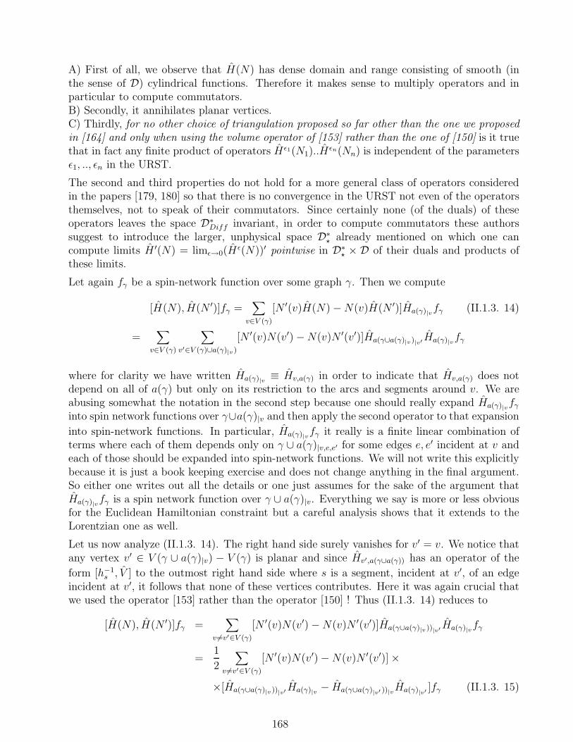
A) First of all, we observe that H(N) has dense domain and range consisting of smooth (inthe sense of D) cylindrical functions. Therefore it makes sense to multiply operators and inparticular to compute commutators.B) Secondly, it annihilates planar vertices.C) Thirdly, for no other choice of triangulation proposed so far other than the one we proposedin [164] and only when using the volume operator of [153] rather than the one of [150] is it truethat in fact any finite product of operators Hǫ1(N1)..H

ǫn(Nn) is independent of the parametersǫ1, .., ǫn in the URST.

The second and third properties do not hold for a more general class of operators consideredin the papers [179, 180] so that there is no convergence in the URST not even of the operatorsthemselves, not to speak of their commutators. Since certainly none (of the duals) of theseoperators leaves the space D∗

Diff invariant, in order to compute commutators these authorssuggest to introduce the larger, unphysical space D∗

⋆ already mentioned on which one cancompute limits H ′(N) = limǫ→0(H

ǫ(N))′ pointwise in D∗⋆ × D of their duals and products of

these limits.

Let again fγ be a spin-network function over some graph γ. Then we compute

[H(N), H(N ′)]fγ =∑

v∈V (γ)

[N ′(v)H(N) −N(v)H(N ′)]Ha(γ)|vfγ (II.1.3. 14)

=∑

v∈V (γ)

∑

v′∈V (γ)∪a(γ)|v )

[N ′(v)N(v′) −N(v)N ′(v′)]Ha(γ∪a(γ)|v )|v′Ha(γ)|vfγ

where for clarity we have written Ha(γ)|v ≡ Hv,a(γ) in order to indicate that Hv,a(γ) does notdepend on all of a(γ) but only on its restriction to the arcs and segments around v. We areabusing somewhat the notation in the second step because one should really expand Ha(γ)|vfγinto spin network functions over γ∪a(γ)|v and then apply the second operator to that expansion

into spin-network functions. In particular, Ha(γ)|vfγ it really is a finite linear combination ofterms where each of them depends only on γ ∪ a(γ)|v,e,e′ for some edges e, e′ incident at v andeach of those should be expanded into spin-network functions. We will not write this explicitlybecause it is just a book keeping exercise and does not change anything in the final argument.So either one writes out all the details or one just assumes for the sake of the argument thatHa(γ)|vfγ is a spin network function over γ ∪ a(γ)|v. Everything we say is more or less obviousfor the Euclidean Hamiltonian constraint but a careful analysis shows that it extends to theLorentzian one as well.

Let us now analyze (II.1.3. 14). The right hand side surely vanishes for v′ = v. We notice thatany vertex v′ ∈ V (γ ∪ a(γ)|v) − V (γ) is planar and since Hv′,a(γ∪a(γ)) has an operator of the

form [h−1s , V ] to the outmost right hand side where s is a segment, incident at v′, of an edge

incident at v′, it follows that none of these vertices contributes. Here it was again crucial thatwe used the operator [153] rather than the operator [150] ! Thus (II.1.3. 14) reduces to

[H(N), H(N ′)]fγ =∑

v 6=v′∈V (γ)

[N ′(v)N(v′) −N(v)N ′(v′)]Ha(γ∪a(γ)|v ))|v′Ha(γ)|vfγ

=1

2

∑

v 6=v′∈V (γ)

[N ′(v)N(v′) −N(v)N ′(v′)] ×

×[Ha(γ∪a(γ)|v ))|v′Ha(γ)|v − Ha(γ∪a(γ)|v′ ))|vHa(γ)|v′

]fγ (II.1.3. 15)

168

where in the second step we used the antisymmetry of the expression [N ′(v)N(v′)−N(v)N ′(v′)]in v, v′. Now the crucial point is that for v 6= v′ ∈ V (γ) the prescription of how to attach thearcs first around v and then around v′ as compared to the opposite may not be the samebecause our prescription depends explicitly on the graph to which we apply it, however, theyare certainly analytically diffeomorphic.

Thus, there exist analytical diffeomorphisms ϕγ,v,v′ preserving γ ∪ a(γ)|v such that

Ha(γ∪a(γ)|v))|v′Ha(γ)|vfγ = U(ϕγ,v,v′)Ha(γ)|v′

Ha(γ)|vfγ (II.1.3. 16)

for any v 6= v′ ∈ V (γ). It follows that

[H(N), H(N ′)]fγ =1

2

∑

v 6=v′∈V (γ)

[N ′(v)N(v′) −N(v)N ′(v′)] ×

×[U(ϕγ,v,v′) − U(ϕγ,v′,v)]Ha(γ)|v′Ha(γ)|vfγ (II.1.3. 17)

where we have used [Ha(γ)|v′, Ha(γ)|v ] = 0 for v 6= v′ since the derivative operators involved act

on disjoint sets of edges.

Expression (II.1.3. 17) is to be compared with the classical formula H(N), H(N ′ = ~H(q−1[(dN)N ′−(dN ′)N ]). The fact that we get a difference between finite diffeomorphism constraint operatorslooks promising at first because for next neighbour vertices v, v′ this could be interpreted as asubstitute for the operator Ha which somehow had to be written in terms of finite diffeomor-phism anyway because we know that the infinitesimal generator dos not exist. Unfortunatelythere are also contributions from pairs v, v′ which are far apart. This we could avoid by specify-ing the choice function more closely in the sense that the arcs aγ,v,e,e′ should, for a given vertexv, not depend on all of γ but only on γv ⊂ γ, the subset of γ consisting of all edges incident atv. But still (II.1.3. 17) does not, at least not obviously, resemble the classical calculation tooclosely because there it is crucial that H(x), H(x′) 6= 0 as x→ x′ while [Ha(γ)|v′

, Ha(γ)|v ] = 0for any v 6= v′.

Certainly then for Ψ ∈ D∗Diff , f ∈ D we have in the URST

Ψ([H(N), H(N ′)]f) := limǫ→0

limǫ′→0

Ψ([Hǫ(N), Hǫ′(N ′)]f) = 0 (II.1.3. 18)

where the limit is again uniform in both Ψ, f . But this would not be surprising even if the righthand side would be a manifset quantization of the right and side (with ~H replaced by U(ϕ)−1H0

and ordered to the outmost left). In other words, in the URST we do not see the differencebetween any operators which are, like (II.1.3. 17), of the form of a difference between twofinite diffeomorphism operators ordered to the outmost left times any other operators. Hereit proves useful to take the effective operator point of view which in fact can detect thosedifferences. Again it requires more work, that is, semiclassical analysis, in order to decidewhether the classical limit of the right hand side of (II.1.3. 17) has anything to do with~H(q−1([(dN)N ′ − (dN ′)N ]). It is worthwhile, however, to point out that (II.1.3. 17) provesthe absence of a strong anomaly. In other words, if (II.1.3. 18) would not hold, then thequantization that we have proposed would be mathematically inconsistent. What is possiblethough is that (II.1.3. 17) could represent a weak anomaly in the sense that the quantumdynamics that H(N) generates is physically inconsistent, that is, the classical dynamics is notreproduced in the classical limit. This is precisely what has to be analyzed in the future and,if true, to find out how to cure the problem.

169

To summarize: The constraint algebra of the Hamiltonian constraints among each other is mathe-matically consistent but possibly has a physical anomaly.

Three remarks are in order:i)In [179, 180] the authors prove a statement similar to (II.1.3. 18) on their space D∗

⋆. The algebra oftheir dual constraint operators becomes Abelean for a large class of operators which even classicallydo not need to be proportional to a diffeomorphism constraint. They then argue that the quantiza-tion method proposed here cannot be correct because it either implies a physical anomaly or, evenworse, that the (dual of the) quantum metric operator qab vanishes identically.

We disagree with this conclusion for two reasons:1)Their limit dual operators are defined by

[H ′(N)Ψ](f) := limǫ→0

Ψ(Hǫ(N)f) (II.1.3. 19)

where convergence is only pointwise, that is, for any δ > 0, Ψ ∈ D∗⋆, f ∈ D there exists ǫ(δ,Ψ, f)

such that|[H ′(N)Ψ](f) − Ψ(Hǫ(N)f)| < δ (II.1.3. 20)

for any ǫ < ǫ(δ,Ψ, f). Thus, while they have blown up D∗Diff to D∗

⋆, their convergence is weaker whenrestricted to D∗

Diff so that it is not easy to compare the two operator topologies (notice that we canalso define a dual operator vial (II.1.3. 19) restricted to D∗

Diff considered as a subspace of D∗, thissubspace is just not left invariant so that we cannot compute commutators of duals). However it isclear that the subspace D∗

⋆ is a sufficiently small extension of D∗Diff in order to make sure that a

much wider class of operators converges in their topology than the class that we have mind for ourtopology since our topology roughly requires that Ψ(Hǫ(N)f) is already independent of ǫ while theirtopology only requires that the ǫ dependence rests in the smearing functions N which are requiredto be smooth at vertices.

Therefore our first conclusion is that it is not surprising that in their topology more operatorsconverge.

Next, let us turn to commutators. In our topology, what is required is that the expression Ψ([Hǫ(N), Hǫ′(N ′)]f)just equals zero independently of how large the graph is on which f depends because we have identifiedHǫ(N) with the continuum operator. In their topology what happens is that unless the operatorH(N) has also the properties B), C) besides A) then one gets for the commutator an expression ofthe form (II.1.3. 15) on which one acts with an element Ψ ∈ D∗

⋆ the result of which is that one gets

([H(N ′)′, H(N)′]Ψ)(fγ) = limǫ→0

limǫ′→0

∑

v∈V (γ)

∑

v′∈V (γ∪aǫ(γ)|v)−V (γ)

[N ′(v)N(v′) −N(v)N ′(v′)] ×

×Ψ[Haǫ′ (γ∪aǫ(γ)|v))|v′Haǫ(γ)|vfγ] (II.1.3. 21)

For the same reason as for Ψ ∈ D∗Diff each evaluation of Ψ that appears on the right hand side

is already independent of ǫ, ǫ′ for any Ψ ∈ D∗⋆ by definition of that space. Therefore the only ǫ, ǫ′

dependence rests in the function [N ′(v)N(v′) −N(v)N ′(v′)]. Now, while each of the roughly |V (γ)|Ψ−evaluations is nonvanishing, since we take the limit pointwise and the N,N ′ are smooth, thelimit vanishes. If we would not have taken pointwise convergence, then for each finite ǫ, ǫ′ we can

170

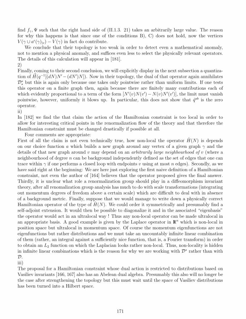
find fγ ,Ψ such that the right hand side of (II.1.3. 21) takes an arbitrarily large value. The reasonfor why this happens is that since one of the conditions B), C) does not hold, now the verticesV (γ ∪ aǫ(γ)|v) − V (γ) in fact do contribute.

We conclude that their topology is too weak in order to detect even a mathematical anomaly,not to mention a physical anomaly, and suffices even less to select the physically relevant operators.The details of this calculation will appear in [181].2)Finally, coming to their second conclusion, we will explicitly display in the next subsection a quantiza-tion of ~H(q−1[(dN)N ′− (dN ′)N ]). Now in their topology, the dual of that operator again annihilatesD∗⋆ but this is again only because one takes only pointwise rather than uniform limits. If one tests

this operator on a finite graph then, again because there are finitely many contributions each ofwhich evidently proportional to a term of the form [N ′(v)N(v′)−N(v)N ′(v′)], the limit must vanishpointwise, however, uniformly it blows up. In particular, this does not show that qab is the zerooperator.ii)In [182] we find the that claim the action of the Hamiltonian constraint is too local in order toallow for interesting critical points in the renormalization flow of the theory and that therefore theHamiltonian constraint must be changed drastically if possible at all.

Four comments are appropriate:First of all the claim is not even technically true, how non-local the operator H(N) is dependson our choice function a which builds a new graph around any vertex of a given graph γ and thedetails of that new graph around v may depend on an arbitrarily large neighbourhood of v (where aneighbourhood of degree n can be background independently defined as the set of edges that one cantrace within γ if one performs a closed loop with endpoints v using at most n edges). Secondly, as wehave said right at the beginning: We are here just exploring the first naive definition of a Hamiltonianconstraint, not even the author of [164] believes that the operator proposed gives the final answer.Thirdly, it is unclear what role a renormalization group should play in a diffeomorphism invarianttheory, after all renomalization group analysis has much to do with scale transformations (integratingout momentum degrees of freedom above a certain scale) which are difficult to deal with in absenceof a background metric. Finally, suppose that we would manage to write down a physically correctHamiltonian operator of the type of H(N). We could order it symmetrically and presumably find aself-adjoint extension. It would then be possible to diagonalize it and in the associated “eigenbasis”the operator would act in an ultralocal way ! Thus any non-local operator can be made ultralocal inan appropriate basis. A good example is given by the Laplace operator in Rn which is non-local inposition space but ultralocal in momentum space. Of course the momentum eigenfunctions are noteigenfunctions but rather distributions and we must take an uncountably infinite linear combinationof them (rather, an integral against a sufficiently nice function, that is, a Fourier transform) in orderto obtain an L2 function on which the Laplacian looks rather non-local. Thus, non-locality is hiddenin infinite linear combinations which is the reason for why we are working with D∗ rather than withD.iii)The proposal for a Hamiltonian constraint whose dual action is restricted to distributions based onVasiliev invariants [166, 167] also has an Abelean dual algebra. Presumably this also will no longer bethe case after strengthening the topology but this must wait until the space of Vasiliev distributionshas been turned into a Hilbert space.

171

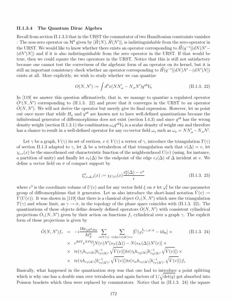
II.1.3.4 The Quantum Dirac Algebra

Recall from section II.1.3.3 that in the URST the commutator of two Hamiltonian constraints vanishes: The non-zero operator on H0 given by [H(N), H(N ′)], is indistinguishable from the zero-operator in

the URST. We would like to know whether there exists an operator corresponding to ~H(q−1[(dN)N ′−(dN ′)N ]) and if it is also indistinguishable from the zero operator in the URST. If that would betrue, then we could equate the two operators in the URST. Notice that this is still not satisfactorybecause one cannot test the correctness of the algebraic form of an operator on its kernel, but it isstill an important consistency check whether an operator corresponding to ~H(q−1[(dN)N ′−(dN ′)N ])exists at all. More explicitly, we wish to study whether we can quantize

O(N,N ′) :=∫d3x(NN ′

,a −N,aN′)qabVb (II.1.3. 22)

In [119] we answer this question affirmatively, that is, we manage to quantize a regulated operatorOǫ(N,N ′) corresponding to (II.1.3. 22) and prove that it converges in the URST to an operatorO(N,N ′). We will not derive the operator but merely give its final expression. However, let us pointout once more that while Ha and qab are known not to have well-defined quantizations because theinfinitesimal generator of diffeomorphisms does not exist (section I.4.3) and since qab has the wrongdensity weight (section II.1.3.1) the combination ωaq

abVb is a scalar density of weight one and thereforehas a chance to result in a well-defined operator for any co-vector field ωa such as ωa = NN ′

,a−N,aN′.

Let γ be a graph, V (γ) its set of vertices, v ∈ V (γ) a vertex of γ, introduce the triangulation T (γ)of section II.1.3 adapted to γ, let ∆ be a tetrahedron of that triangulation such that v(∆) = v, letχǫ,v(x) be the smoothened out characteristic function of the neighbourhood U(v) (using, for instance,a partition of unity) and finally let sI(∆) be the endpoint of the edge eI(∆) of ∆ incident at v. Wedefine a vector field on σ of compact support by

ξaǫ,v,∆,I(x) := χU(v)(x)saI(∆) − va

ǫ(II.1.3. 23)

where ǫ3 is the coordinate volume of U(v) and for any vector field ξ on σ let ϕξt be the one-parametergroup of diffeomorphisms that it generates. Let us also introduce the short-hand notation V (v) :=V (U(v)). It was shown in [119] that there is a classical object Oγ(N,N

′) which uses the triangulationT (γ) and whose limit, as γ → σ, in the topology of the phase space coincides with (II.1.3. 22). Thequantizations of these objects define densely defined operators O(N,N ′) with consistent cylindricalprojections Oγ(N,N

′) given by their action on functions fγ cylindrical over a graph γ. The explicitform of these projections is given by

O(N,N ′)fγ = −i16ǫijkǫilmhℓ2p

∑

v∈V (γ)

∑

v(∆)=v(∆′)=v

[U(ϕξǫ,v,∆′,Rǫ − idH] × (II.1.3. 24)

× ǫRST ǫNPQ[N(v)N ′(sN(∆)) −N(sN (∆))N ′(v)] ×× tr(τjheP (∆)[h

−1eP (∆),

√V (v)])tr(τkheQ(∆)[h

−1eQ(∆),

√V (v)]) ×

× tr(τlheS(∆′)[h−1eS(∆′),

√V (v)])tr(τmheT (∆′)[h

−1eT (∆′),

√V (v)])fγ

Basically, what happened in the quantization step was that one had to introduce a point splitting

which is why one has a double sum over tetrahedra and again factors of 1/√

det(q) got absorbed into

Poisson brackets which then were replaced by commutators. Notice that in (II.1.3. 24) the square

172

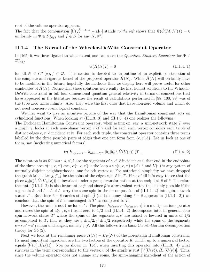
root of the volume operator appears.

The fact that the combination [U(ϕξǫ,v,∆′,Rǫ − idH] stands to the left shows that Ψ(O(M,N ′)f) = 0

uniformly in Ψ ∈ D∗Diff and f ∈ D for any N,N ′.

II.1.4 The Kernel of the Wheeler-DeWitt Constraint Operator

In [165] it was investigated to what extent one can solve the Quantum Einstein Equations for Ψ ∈D∗Diff

Ψ(H(N)f) = 0 (II.1.4. 1)

for all N ∈ C∞(σ), f ∈ D. This section is devoted to an outline of an explicit construction ofthe complete and rigorous kernel of the proposed operator H(N). While H(N) will certainly haveto be modified in the future, hopefully the methods that we display here will prove useful for othercandidates of H(N). Notice that these solutions were really the first honest solutions to the Wheeler-DeWitt constraint in full four dimensional quantum general relativity in terms of connections thathave appeared in the literature because the result of calculations performed in [98, 100, 99] was ofthe type zero times infinity. Also, they were the first ones that have non-zero volume and which donot need non-zero cosmological constant.

We first want to give an intuitive picture of the way that the Hamiltonian constraint acts oncylindrical functions. When looking at (II.1.3. 3) and (II.1.3. 4) one realizes the following :The Euclidean Hamiltonian Constraint operator, when acting on, say, a spin-network state T overa graph γ, looks at each non-planar vertex v of γ and for each such vertex considers each triple ofdistinct edges e, e′, e incident at it. For each such triple, the constraint operator contains three termslabelled by the three possible pairs of edges that one can form from e, e′, e. Let us look at one ofthem, say (neglecting numerical factors)

tr([hα(v;e,e′) − hα(v;e,e′)−1 ]hs[h−1s , V (U(v))])T . (II.1.4. 2)

The notation is as follows : s, s′, s are the segments of e, e′, e incident at v that end in the endpointsof the three arcs a(v; , e, e′) etc., α(v; e, e′) is the loop s a(v; e, e′) (s′)−1 and U(v) is any system ofmutually disjoint neighbourhoods, one for ech vertex v. For notational simplicity we have droppedthe graph label. Let j, j′, j be the spins of the edges e, e′, e in T . First of all it is easy to see that thepiece hs[h

−1s , V (Uǫ0(v))] is invariant under a gauge transformation at the endpoint p of s. Therefore

the state (II.1.4. 2) is also invariant at p and since p is a two-valent vertex this is only possible if thesegments s and e − s of e carry the same spin in the decomposition of (II.1.4. 2) into spin-networkstates T ′. But since e − s carries still spin j (no holonomy along e − s appears in (II.1.4. 2)) weconclude that the spin of e is unchanged in T ′ as compared to T .

However, the same is not true for e, e′ : The piece [hα(v;e,e′)−hα(v;e,e′)−1 ] is a multiplication operatorand raises the spin of a(v; , e, e′) from zero to 1/2 and (II.1.4. 2) decomposes into, in general, fourspin-network states T ′ where the spins of the segments s, s′ are raised or lowered in units of 1/2as compared to T , that is, they are j ± 1/2, j′ ± 1/2 respectively while the spins of the segmentse−s, e′−s′ remain unchanged, namely j, j′. All this follows from basic Clebsh-Gordan decompositiontheory for SU(2).

Next we look at the remaining piece H(N) + HE(N) of the Lorentzian Hamiltonian constraint.Its most important ingredient are the two factors of the operator K which, up to a numerical factor,equals [V (σ), HE(1)]. Now as shown in [164], when inserting this operator into (II.1.3. 4) whatsurvives in the term corresponding to the vertex v of the graph is just [V (U(v)), HE(U(v))]. Thus,since the volume operator does not change any spins, the spin-changing ingredient of the action of

173

the remaining piece of H(N) at v are two successive actions of HE(U(v)) as just outlined.

In summary, the Hamiltonian constraint operator has an action similar to a fourth order polyno-mial consisting of creation of annihilation operators. What is being created or annihilated are thespins of edges of a graph (notice that an edge with spin zero is the same as no edge at all).

Let us now look at this action in more detail. We will restrict attention only to the Euclideanpiece, for the more complicated full action see [165].Notice that the Euclidean constraint operator creates edges of a special kind, called extraordinaryedges, namely the arcs a = a(v; e, e′). What is special about them is that they end in planar verticeswhich are either bi- or tri-valent. If they are tri-valent then, moreover, the vertex is the intersectionof the two analytical edges a, e where a just ends on an interiour point of e. Moreover, let e, e′ be theedges on which a ends. Then the analytical extensions of e, e′ end in at least one point and the twopossible earliest of their intersection points away from a∩ e, a∩ e′ are, together with these analyticalextensions, non-planar vertices of γ. However, not only are these edges special, also the spin theycarry is special, namely the arc a carries always spin 1/2. We will continue to call this whole set ofextraordinary structures an extraordinary edge.

The special nature of these edges allows to classify the full set of labels S of spin-network states,called spin-nets, as follows. Denote by S0 ⊂ S, called sources, the set of spin-nets, corresponding tographs with no extraordinary edges at all.

From these sources one constructs iteratively derived sets Sn(s0), n = 0, 1, 2, .. for each sources0 ∈ N0, called spin-nets of level n based on s0. Put S0(s0) := s0 and define Sn+1(s0) as follows: Take each s ∈ Sn(s0), compute HE(N)Ts for all possible lapse functions N , decompose it intospin-network states and enter the appearing spin-nets into the set Sn+1(s0).

In [165] it is shown that the sets Sn(s0),Sn′(s′0) are disjoint unless s0 = s′0 and n = n′. It iseasy to see that the complement of the set of sources S0 = S − S0 coincides with the set of derivedspin-nets of level greater than zero. Moreover, for each s ∈ N there is a unique integer n and aunique source s0 such that s ∈ Sn(s0).

The purpose for doing all this is, of course, that this classification leads to a simple constructionof all rigorous solutions of the Euclidean Hamiltonian constraint based on the observation that

HE(N) · spanTss∈Sn(s0) ⊂ spanTss∈Sn+1(s0) . (II.1.4. 3)

Since a solution Ψ of (II.1.4. 1) is a diffeomorphism invariant distribution in D∗Diff we define first

[Sn(s0)] := [s]s∈Sn(s0) where [s] is the label for the diffeomorphism invariant distribution T[s] (recallsection I.4.3). We can now make an ansatz for a basic solution of the form

Ψ := Ψ[s0],~n :=N∑

k=1

∑

[s]∈[Snk(s0)]

c[s]T[s] (II.1.4. 4)

with complex coefficients c[s] which are to be determined from the Quantum Einstein Equations

(II.1.4. 1). Now from (II.1.4. 4) it is clear that Ψ[s0],[~n](HE(N)Ts) can be non-vanishing if and only if[s] ∈ [Snk−1(s0)] for some k = 1, .., n, say k = l. Choose a representant s ∈ [s] and let γ be the graph

underlying s and V (γ) its set of vertices. We then find, writing HE(N) =∑v∈V (γ)N(v)HE(v), that

Ψ[s0],~n(HE(N)Ts) =∑

[s′]∈[Snl(s0)]

c[s′]∑

v∈V (γ)

N(v)T[s′](HE(v)Ts) (II.1.4. 5)

174

should vanish for any choice of lapse function N(v). Since N(v) can be any smooth function we findthe condition that

Ψ[s0],~n(HE(N)Ts) =∑

[s′]∈[Snl(s0)]

c[s′]T[s′](HE(v)Ts) = 0 (II.1.4. 6)

should vanish for each choice of the finite number of vertices v ∈ V (γ) and for each of the finitenumber of spin-nets s ∈ Snl−1(s0). This follows from the fact that the numbers T[s′](HE(v)Ts) arediffeomorphism invariant and therefore do not actually depend on v itself but only on the diffeo-morphism invariant information that is contained in the graph γ together with the vertex v singledout.

Therefore, (II.1.4. 6) is a finite system of linear equations for the coefficients c[s′]. As the cardinal-ity of the sets Sn(s0) exponentially grows with n this system is far from being overdetermined and wearrive at an infinite number of solutions. The most general solution will be a linear combination ofthe elementary solutions (II.1.4. 6). Qualitatively the same result holds for the Lorentzian constraint[165], however, it is more complicated because coefficients from different levels get coupled and soone gets solutions labelled also by the highest level that was used (possibly one has to allow all levels,that is, the highest level is always infinity). Nevertheless it is remarkable how the solution of theQuantum Einstein Equations is reduced to an exercise in finite-dimensional linear algebra (althoughthe computation of the coefficients T[s′](HE(v)Ts) is far from easy, see, e.g., [183] which, although

the authors restrict to tri-valent graphs and HE(N) only, is already rather involved). On the otherhand, it is expected that physically interesting solutions will actually be infinite linear combinationsof coupled solutions, that is, solutions of infinite level, an intuition coming from [184].

Notice that the solutions (II.1.4. 6) are bona fide elements of D∗Diff and therefore give, for

the first time, rigorously defined solutions to the diffeomorphism and the Hamiltonian constraintof full, four-dimensional Lorentzian Quantum General Relativity in the continuum, subject to thereservation that we still have to prove that the classical limit of this theory in fact is general relativity.One should now organize these solutions into a Hilbert space such that adjointness and canonicalcommutation relations of full Dirac observables are faithfully implemented. Since group averagingdoes not work for open algebras, there is no good proposal at this point for how to do that and is avery important open research problem.

II.1.5 Further Related Results

We list here further results that are directly connected to the issues that we have touched upon inthis section already.

II.1.5.1 Generator of the Wick Transform

In principle we could dispense with the rigorous construction of the Wick transform since we couldwork entirely with the operators (II.1.3. 3) and (II.1.3. 4) rather than with the modified ones de-scribed in this subsection. However, since the availability of a complex connection representationcould be conceptually important in particular when making contact with the path integral formula-tion, we will make a short digression on available first ansatze for how to get there.

Recall that the generator of the Wick transform C is given, up to numerical factors, by i[V (σ), HE(1)].One would like to invoke the spectral theorem in order to define its exponential and it is thereforemotivated to have an at least symmetric operator HE(1). This, however, is not the case the wayHE(1) is defined : take for example s ∈ S0, s

′ ∈ S1(s) such that < Ts′, HE(1)Ts > 6= 0, but then

< Ts, HE(1)Ts′ > = 0 by definition of S0. Of course, one can symmetrize the operator by defining

175

the matrix elements of the symmetric operator to be the half the sum of the matrix elments of theunsymmetric operator plus the transpose of its complex conjugate. This operator is also well-definedbut in [165] we did not succeed in proving existence of self-adjoint extensions of it. What works isthe following : one marks the extraordinary edges by taking them to be smooth but not analytical.This way it becomes possible to tell whether a given state was obtained by the action of the con-straint on a function cylindrical over a piecewise analytical graph. Then the repeated action of theconstraint adds always the same smooth extraordinary edge a(v; e, e′) to the graph and this turnsthe operator into a symmetric one when factor-ordering its expression symmetrically. The formalismis not disturbed by the fact that one leaves the purely analytical category of graphs. The so sym-metrized operator is free of mathematical anomalies as well but the structure of its solutions becomesmore complicated. One can then invoke von Neumann’s theorem (that says that if a densely definedsymmetric operator commutes on its domain with a conjugation operator that preserves its domainthen there exist self-adjoint extensions) to show that HE(N) and in fact also C have self-adjointextensions. (A conjugation operator is a bounded, anti-linear operator which squares to the iden-tity). This method of proof does not work, however, for the constraint H(N) because the Lorentzianoperator is a sum consisting of two operators which are symmetric and have self-adjoint extensionsbut it is unclear whether they have extensions to the same domain (the explicit extensions are noteven known although it is likely that all operators in question are essentially self-adjoint in whichcase the answer would be given by their closure).

In any case, we could in principle define self-adjoint operators HE(N), C and define the operatorWt := exp(−tC) by its spectral resolution. Then, according to the philosophy of the Wick transformof section II.1.1 we should analytically continue the operator W−1

t HE(N)Wt and define it to be theLorentzian Hamiltonian constraint. The problem is that the spectrum of C is far from known andit is not even clear, although extremely likely, that HE(N) and C can be extended as self-adjointoperators to the same domain. A method of proof, as sketched in [165], could probably be based onNelson’s analytic vector theorem but the proof was not completed there.

II.1.5.2 Testing the New Regularization Technique by Models of Quantum Gravity

Presently there are two positive tests for the quantization procedure that we applied to the Hamil-tonian constraint, namely Euclidean 2 + 1 gravity [184] and isotropic and homogeneous BIanchicosmologies quantized in a non-standard fashion [185].

The first model is a dimensional reduction of 3 + 1 gravity which one can formulate also as aquantum theory of SU(2) connections and su(2) electric fluxes with precisely the same algebraicform of all constraints. Hence, one can introduce the full mathematical structure of A, µ0,H0 as well

as the quantum constraints Gj = DaEaj , Va = F j

abEbj , HE = F j

abEakE

bl ǫjkl/

√det(q) the only difference

with the Lorentzian 3 + 1 theory being that now indices a, b, c, .. = 1, 2 have range in one dimensionless and that there is only the Euclidean constraint.

The second model is 3+1 Lorentzian gravity but instead of performing the usual Killing reductionone looks for (distributional) states in the full Hilbert space H0 of the theory which are compatiblewith the Killing symmetries of the model.

In both models one then follows step by step the regularization procedure outlined in sectionsII.1.2,II.1.3. The outcomes are as follows:

• Euclidean 2+1 GravityThe quantization of 2+1 general relativity is an exhaustively studied problem (see, e.g., [186,187, 188, 189, 190, 191, 192], third and fourth references in [103] and references in all of those).Several different quantization techniques have been applied and were shown to give consistent

176

results. The reader might wonder why 2+1 Euclidean quantum gravity should serve as atest model for 3+1 Lorentzian quantum gravity. The reason for this is that, as pointed outin [191, 192], the Hamiltonian formulation of 2+1 gravity via connections leads to the non-compact gauge group SU(1, 1) for three-metrics of Lorentzian signature while for three-metricsof Euclidean signature we have the same compact gauge group as in Lorentzian 3+1 gravity,namely SU(2). Thus, in order to maximally simulate the 3+1 theory, we should considerEuclidean 2+1 gravity.

However, in order to maximally test the new technique introduced in sections II.1.2, II.1.3 andthe constraints of the 3+1 theory one has to develop techniques different from those that peoplenormally employ in 2+1 gravity which make [184] of interest by itself. In particular, it containsa full fledged derivation of the 2 + 1 volume operator. The reason is the following:Pure 2 + 1 gravity on a Riemann surface of some fixed genus is a topological field theory,that is, there are only finitely many degrees of freedom. This can be easily seen from thefact that we have six canonical pairs and six first class constraints. When the metric qab isnon-degenerate, the Diffeomorphism and Hamiltonian constraint together are equivalent to theFlatness Constraint Cj := ǫabF j

ab = 0. Almost exclusively the theory is quantized using Cjrather than Va, H , see in particular [187] and reference three and four of [103]. But of coursewe must use Va, H in order to test the 3 + 1 theory appropriately.

The result is that all steps of the quantization programme can be carried up to and includingthe construction of the full solution space to all constraint. The structure of that solutionspace is as complicated as in the 3+1 theory, therefore it is not easy to find a suitable physicalinner product. However, one finds that the full space of solutions to the flatness constraintis contained as a subspace in the space of solutions to the Diffeomorphism and Hamiltonianconstraint. Therefore, the validity of the quantization method is confirmed in this model.Futhermore, the curvature operator Fab (which of course becomes substituted by a holonomyalong contractible loop) must be ordered to the most left. Thus, ordering is important here,in particular the Hamiltonian constraint is by far not even symmetric in that ordering. Aninner product on that subspace of the full solution space is then suggested to be usual productintroduced in [187]. The full solution space of the Diffeomorphism and Hamiltonian constraintis much larger which could be related to the fact that it contains a huge number of states withvanishing volume [184], however, this speculation is yet unconfirmed. What to do with zerovolume states (degenerate three metrics) in 3 + 1 connection quantum gravity has always beena puzzle [186].

• Isotropic, Homogeneous Bianchi CosmologiesIn an outstanding series of papers [185] Bojowald has introduced a method for embedding thequantum theory of a Killing – or dimensionally reduced model of a given field theory of con-nections into the quantum theory of the full unreduced theory. Paraphrasing somewhat theprocedure, roughly what happens is the following:In contrast to the usual mini (midi) superspace quantization procedure of first reducing theclassical theory by the Killing symmetry and then quantizing the resulting reduced theory, hereone starts with the Hilbert space of the full unreduced theory and imposes the Killing symme-try on states. Since the Killing symmetry group is in a sense a subgroup of the diffeomorhismgroup it is clear that one gets symmetric (distributional) states by a kind of group averagingprocedure together with a natural group averaging inner product. One then “projects” the con-straint operators of the full theory, regularized by the same technique as in section II.1.3, on thespace of symmetric states. The method is very general but most is known for the isotropic and

177

homogeneous Bianchi models and has culminated in a series of papers entitled “Loop QuantumCosmology I – IV” plus successors thereof [185]. The results are indeed spectacular:

1) Absence of Initial SingularityLet us take as a detector for the big bang singularity in a Friedman – Robertson – Walkermodel the divergence of the inverse scale factor 1/a at a = 0. In quantum theory the bigbang singularity evaporates !!! It is simply not there. The technical reason is as follows:The function 1/a is classically a negative power of the volume functional which we candisplay as the Poisson bracket between a positive power of the volume functional and aholonomy by using the same key identities that were employed in section II.1.2. Nowone simply replaces the Poisson bracket by a commutator exactly as we havedone in the full theory and in that very precise sense, the results by Bojowaldconfirm the validity of our quantization technique of [164]. The crucial fact isnow that the commutator cannot blow up at low volume. Even better, one can show thatthe quantization of 1/a is a positive semi-definite operator which is bounded from above !Thus, in loop quantum cosmology one of the dreams about quantum gravity, that it curesclassical singularities seems to come true.

2) Rapid Convergence to the Classical RegimeOne might imagine that a quantization of 1/a with such bizarre properties should have aspectrum far off the classcal curve a 7→ 1/a. However, this is far from true: As one canimagine, (linear combinations of symmetric subsets of) spin network states diagonalizethe inverse scale factor operator and its spectrum is purely discrete. Already for spins aslow as j > O(10) the spectrum lies exaclty on the classical curve.

3) Discrete Time EvolutionThe scale factor itself makes a good time observable in the present model. As the solutionalgorithm for the Hamiltonian constraint of the full theory, section II.1.4, already indicates,the time evolution becomes discrete and can be solved in closed form. Amazingly, giveninitial data one can quantum evolve through the classical singularity to negative times.

4) No Boundary Conditions NecessaryWhen analyzing the solution space of the quantum evolution equation (Wheeler – De-witt equation) one discovers that there is a unique solution with the correct semiclassicalproperties. Thus, one does not need to carefully adjust the boundary condition on theinitial state [186] in order to get a state today with the desired properties, the theory itselfchooses that state!

One should, of course, consider more examples and transfer these results to the full theory in orderto gain confidence into the quantization method, ultimatively a semiclassical analysis is unavoidable,however, these two results described are hopefully promising enough in order to take the proposalfor the regularization of the Hamiltonian constraint proposed sufficiently serious.

II.1.5.3 Quantum Poincare Algebra

In [157] an investigation was started in order to settle the question whether H0 supports the quan-tization of the ADM energy surface integral

EADM(N) = −2

κ

∫

∂σdSa

N√det(q)

Eaj ∂bE

bj (II.1.5. 1)

178

for an asymptotically flat spacetime M (here ∂σ corresponds to spatial infinity i0 in the Penrosediagramme describing the conformal completion of M). It should be stressed that (II.1.5. 1) is thevalue of the graviatational energy (at unit lapse N = 1) only when the constraints are satisfied,otherwise one has to add to (II.1.5. 1) the Hamiltonian constraint H(N). In particular one has touse HADM(N) = H(N)+EADM (N) in order to compute the equations of motion. If N is, say of rapiddecrease, then HADM(N) = H(N) generates gauge transformations (time reparameterizations), if itis asymptotically constant then it generates symmetries. There are nine more surface integrals of thetype (II.1.5. 1) and together they generate the asymptotic Poincare algebra. They are the only tenDirac obeservables known for full, Lorentzian, asymptotically flat gravity in four dimensions. For adiscussion of these and related issues, see e.g. [87] and references therein.

In [157] we were only able to cover time translations (II.1.5. 1), spatial translations and spatialrotations. Boosts, which are much harder to define, were not considered there but there is no principalproblem to do so. We will focus here only on the quantization of (II.1.5. 1) for reasons of brevity.The method of regularization and quantization completely parallel those displayed in sections II.1.2,II.1.3 and will not be repeated here. The only new element that goes into the classical regularizationis the exploitation of the fall off conditions on the classical fields, in particualr that A = O(1/r2) inan asymptotic radial coordinate. This enables one to replace, effectively, in (II.1.5. 1) ∂bE

bj by the

gauge invariant quantity Gj = DbEbj in (II.1.5. 1), that is, the Gauss constraint. At first sight one

is tempeted to set it equal to zero. However, a detailed analysis shows that for the Gauss constraintto be functionally differentiable, its Lagrange multiplier must fall off as 1/r2 which means that theGauss constraint does not need to hold at ∂σ. Thus, it would be physically incorrect to requireGj = 0 at ∂σ, in other words, quantum states do not need to be gauge invariant at ∂σ or, putdifferently, the motions generated by Gj at ∂σ are not gauge transformations but symmetries.

The final answer is (EADM = EADM(1))

EADMfγ = −2mp

∑

v∈V (γ)∩∂σ

ℓ3p

VvRjvR

jvfγ (II.1.5. 2)

where Rjv =

∑f(e)=v R

je, Vv = limRv→v V (Rv) and x 7→ Rx is an open region valued function with

x ∈ Rx. The operator (II.1.5. 2) is defined actually on an extension of H0 which allows for edges thatare not compactly supported. Moreover we must require that 1) for each v ∈ γ ∩ ∂σ the eigenvaluesof Vv are non-vanishing and that 2) e ∩ ∂σ is a discrete set of points for every e ∈ E(γ). We haveassumed w.l.g. that all edges with e ∩ ∂σ 6= ∅ are of the “up” type with respect to the surface ∂σ.

Under these assumptions one can show the following:

i) Positive Semi-Definiteness(II.1.5. 2) defines a self-consistent family of essentially self-adjoint, positive semi-definite op-erators. This is like a quantum positivity of energy theorem but it rests heavily on the twoassumptions 1) and 2) made above whose physical origin is poorly understood.

ii) Fock Space InterpretationSince the volume operator is gauge invariant, it follows that it commutes with the Laplacian∆v = (Rj

v)2 and therefore we can simultaneously diagonalize these operators. It is clear that

the eigenstates are certain linear combinations of spin-network states and the eigenvalues areof the form jv(jv + 1)/λv (where λv is a volume eigenvalue) times mp. Thus we can completethe intuitive picture that the Hamiltonian constraint gave us: while the constraint changesthe spin quantum numbers, the energy is diagonal in it in very much the same way as theannihilation and creation operators of quantum mechanics change the occupation number of

179

an energy eigenstate. We may thus interpret the spin quantum numbers as occupation numbersof a non-linear Fock representation. In quantum field theory we label Fock states by occupationnumbers nk for momentum modes k. Here we have occupation numbers je for “edge modes” e.

iii) Spectral PropertiesThe eigenvalues are discrete and unbounded from above but in contrast to the geometry opera-tors there is no energy gap. Rather there is an accumulation point at zero because [∆v, Vv] = 0(we can choose the state to be very close to being gauge invariant but to have arbitrarily largevolume). This is to be expected on physical grounds because we should be able to detectarbitrarily soft gravitons at spatial infinity.

iv) Quantum Dirac Observable and Schrodinger equation(II.1.5. 2) trivially commutes with all constraints (since diffeomorphisms ϕ and lapses N thatgenerate gauge transformations are trivial (identity and zero) at ∂σ) and therefore representsa true quantum Dirac observable. In principle we can now solve “the problem of time” since aphysically meaningful time parameter is selected by the one parameter unitary groups generatedby EADM , in other words, we have a Schrodinger equation

− ih∂Ψ

∂t= EADMΨ (II.1.5. 3)

Actually in [157] concepts that go beyond H0 were needed and introduced heuristically. They gounder the name “Infinite Tensor Product Extension” and were properly defined only later in [136].They will be discussed briefly in section II.3.2.

180

II.2 Extension to Standard Matter

The exposition of section II.1 would be unserious if we would not be able to extend the frameworkalso to matter, at least to the matter of the standard model. This is straightforward for gauge fieldmatter, however for fermionic and Higgs matter one must first develop a background independentmathematical framework [194]. We will discuss the essential steps in the next subsection and thensketch the quantization of the matter parts of the total Hamiltonian constraint in the section afterthat, see [193] for details.

We should point out that these representations are geared towards a background independentformulation. The matter Hamiltonian operator of the standard model in a background spacetimeis not carried by these representations. They make sense only if we couple quantum gravity. Also,while we did not treat supersymmetric matter explicitly, the following exposition reveals that it isstraightforward to extend the formalism to Rarita – Schwinger fields.

II.2.1 Kinematical Hilbert Spaces for Diffeomorphism Invariant Theo-

ries of Fermionic and Higgs Fields

First attempts to couple quantum field theories of fermions to quantum general relativity gravitywere made in the pioneering work [195]. However, this paper was still written in terms of thecomplex-valued Ashtekar variables for which the kinematical framework was missing. Later on [196]appeared in which a kinematical Hilbert space for diffeomorphism invariant theories for fermions wasproposed which were coupled to arbitrary gauge fields and real-valued Ashtekar variables using thekinematical framework of section I.2. Also, the diffeomorphism constraint was solved there but notthe Hamiltonian constraint. However, that fermionic Hilbert space did implement the correct realityconditions for the fermionic degrees of freedom only for a subset of all kinematical observables. In[194] we removed this problem by introducing new fermionic variables, so-called Grassmann-valuedhalf-densities and also extended the framework to Higgs fields. This section is accordingly subdividedinto one section each for the fermionic and the Higgs sector respectively and in the third section wecollect results and define the most general gauge and diffeomorphism invariant states of connections,fermions and Higgs fields.

II.2.1.1 Fermionic Sector

We will take the fermionic fields to be Grassmann-valued, see [197, 198] for a mathematical intro-duction into these concepts. Furthermore, the Grassmann field ηAµ is a scalar with respect to diffeo-morphisms of σ which carries two indices, A,B,C, .. = 1, 2 and µ, ν, ρ = 1, .., dim(G) correspondingto the fact that it transforms according to the fundamental representation of SU(2) and the definingrepresentation of the compact, connected, unimodular gauge group G of a Yang-Mills gauge theoryto which it may couple. This can be generalized to arbitrary representations of SU(2) × G but werefrain from doing that for the sake of concreteness. Notice that it is no loss of generality to restrictourselves to only one helicity of the fermion as we can always perform a canonical transformation(iσA

′, σA′) → (iǫAB

′σB′ , ǫAB′ σB

′) =: (iηA, ηA). We will restrict to only one fermionic species in order

not to clutter the formulae.It turns out that the real-valued action in Hamiltonian form for any diffeomorphism invariant

theory of fermions is given by

SF =∫

Rdt∫

σd3x(

i

2

√det(q)[ηAµηAµ − ˙η

AµηAµ] − [more]) (II.2.1. 1)

181

where “more” stands for various constraints and possibly a Hamiltonian and det(q) is the determinantof the gravitational three-metric which appears because in four spacetime dimensions one needs ametric to define a diffeomorphism invariant theory of fermions. Notice that (II.2.1. 1) is real valuedwith respect to the usual involution (θ1..θn)

∗ = θn..θ1 for Grassmann variables θ1, .., θn since indicesA, µ are raised and lowered with the Kronecker symbol (the involution is just complex conjugationwith respect to bosonic variables).

The immediate problem with (II.2.1. 1) is that it is not obvious what the momentum πAµ

conjugate to ηAµ should be. One strategy would be to integrate the second term in (II.2.1. 1) by parts(the corresponding boundary term being the generator of the associated canonical transformation)

and to conclude that it is given by i√

det(q)ηAµ. However, there is a second term from the integration

by parts given by iEai e

iaη

AµηAµ which after a further integration by parts combines with the symplecticpotential of the real-valued Ashtekar variables to the effect that Aia is replaced by (CAia) = Aia −ieiaη

AµηAµ (recall that Eai is the momentum conjugate to Aia). This is bad because the connection

is now complex-valued and the techniques from section I.2 do not apply any longer so that we arein fact forced to look for another method. The authors of [196] also noticed this subtlety in the

following form: If one assumes that the connection is still real-valued while π = i√

det(q)η is takenas the momentum conjugate to η then one discovers the following contradiction: By assumption wehave the classical Poisson bracket π(x), A(y) = 0. Taking the involution of this equation results

in 0 = −iη(x)√

det(q)(x), A(y) 6= 0. If we, however, insert instead of A the complex variable (CA)

into these equations then in fact there is no contradiction as was shown in [194].The idea of how preserve the real-valuedness of Aia and to simplify the reality conditions on the

fermions is as follows : Notice that if we define the Grassmann-valued half-density

ξAµ := 4

√det(q)ηAµ (II.2.1. 2)

then (II.2.1. 1) in fact equals

SF =∫

Rdt∫

σd3x(

i

2[ξAµξAµ − ˙ξ

AµξAµ] − [more]) (II.2.1. 3)

without picking up a term proportional to d det(q)/dt. Thus the momentum conjugate to ξAµ andthe reality conditions respectively are simply given by

πAµ = iξAµ and (ξ)∗ = −iπ, (π)∗ = −iξ . (II.2.1. 4)

The fact that ξ, π are half densities may seem awkward at first sight but it does not cause anyimmediate problems. Also, recall that “half-density-quantization” is a standard procedure in thetheory of geometric quantization of phase spaces with real polarizations [51].

It is in fact possible to base the quantization on the half-density ξ as a quantum configurationvariable as far as the solution to the Gauss constraint is concerned. Namely, as has been pointed outby many (see, e.g., [195]) an example for a natural, classical, gauge invariant observable is given by

Pe(ξ, A,A) := ξAµ(e(0))CAµ,Cρ1 (he(A))CD(π(he(A)))ρσC

Dσ,Bν2 ξBν(e(1)) (II.2.1. 5)

where the notation is as follows : By (A, he, π(he)) and (A, he, π(he)) respectively we denote (con-nection, holonomy along an edge e, irreducible representation evaluated at the holonomy) of thegravitational SU(2) and the Yang-Mills gauge group G respectively. The matrices CAµ,Bν are pro-jectors on singlet representations of the decomposition into irreducibles of tensor product repre-sentations that appear under gauge transformations on both ends of the path [0, 1] ∋ t → e(t)

182

and the irreducible representation π has to be chosen in such a way that a singlet can occur. Forexample, if G = SU(N) then we can choose π to be the complex conjugate of the defining represen-tation. In particular, if G = SU(2) as well we can take π to be the fundamental representation andCAµ,Cρ

1 = ǫACǫµρ, CDσ,Bν2 = δDBδσν . For more general groups we may have to take more than one

spinor field at each end of the path in order to satisfy gauge invariance.All this works fine until it comes to diffeomorphism invariance : notice that the objects (II.2.1.

5) behave strangely under a diffeomorphism ϕ, namely ϕ · Pe = Pϕ(e)(Jϕ(e(0))Jϕ(e(1)))−1/2 whereJϕ(x) = | det(∂ϕ(x)/∂x)| is the Jacobian. Since there are analyticity preserving diffeomorphismswhich leave e invariant but such that, say, Jϕ(e(0)) can take any positive value it follows that theaverage of Pe over diffeomorphisms is meaningless. We are therefore forced to adopt another strategy.

The new idea [194] is to “dedensitize” ξ by means of the δ-distribution δ(x, y) which itself trans-forms as a density of weight one in either argument. Let θ(x) be a smooth Grassmann-valued scalar(we drop the indices Aµ) and we define ξ(x) not to be a smooth function but rather a distribution(already classically). Let δx,y = 1 for x = y and zero otherwise (a Kronecker δ, not a distribution).

Then on the space of test functions of rapid decrease the distribution√δ(x, y)δ(z, y) is well-defined

and equals δx,zδ(x, y) [194]. As shown in [194] the following transformations (and corresponding onesfor the complex conjugate variables)

θ(x) :=∫

σd3y

√δ(x, y)ξ(y) (II.2.1. 6)

ξ(x) =∑

y∈σδ(x, y)θ(y) (II.2.1. 7)

are canonical transformations between the symplectic structures defined by the symplectic potentialsi∫σ d

3xξ(x)ξ(x) and i∑x∈σ θ(x)θ(x) respectively. Notice that (II.2.1. 6) makes sense precisely when

ξ is a distributional half-density and in fact one can show that ξ = η 4

√det(q) will precisely display

such a behaviour (at least upon quantization) since√

det(q) becomes an operator valued distribution

proportional to the δ distribution (recall the formula for the volume operator). The non-trivialanti-Poisson brackets in either case are given by

ξ(x), ξ(y)+ = −iδ(x, y) and θ(x), θ(y)+ = −iδx,y . (II.2.1. 8)

In summary, we conclude that we can base the quantization of the fermionic degrees of freedom onθ as a configuration variable with conjugate momentum and reality structure given by

πAµ = iθAµ and (θ)∗ = −iπ, (π)∗ = −iθ . (II.2.1. 9)

We now have to develop integration theory. This will be based, of course, on the Berezin “integral”[197, 198]. Let S(x) be the superspace underlying the 2d fermionic configuration degrees of freedomθAµ(x) for any x ∈ Σ where d = 2 dim(G). Of course, all these spaces are just copies of a single spaceS. This superspace can be turned into a trivial σ-algebra B(x) consisting of S(x) and the empty set.On B(x) one can define a probability “measure” dmx with the additional property that it is positiveon “holomorphic” functions (that is, those which depend θ(x) only and not on θ(x)) in the sensethat

∫S dmxf(θ(x))∗f(θ(x)) ≥ 0 where equality holds if and only if f = 0. This measure is given by

dm(θ, θ) =∏

Aµ

(1 + θAµθAµ)dθAµdθAµ (II.2.1. 10)

and dmx = dm(θ(x), θ(x)).Let now S := ×x∈σSx be the fermionic quantum configuration space with σ-algebra B given by

183

the direct product of the B(x). The Kolmogorov-theorem [58] for uncountable direct products ofprobability measures ensures that

dµF (θ, θ) := ⊗x∈σdmx (II.2.1. 11)

is a rigorously defined probability measure on S. It can be recovered as the direct product limit(rather than projective limit) from its finite dimensional joint distributions defined by cylindricalfunctions. Here a function F on S is said to be cylindrical over a finite number of points x1, .., xnif it is a function only of the finite number of degrees of freedom θ(x1), .., θ(xn) and their complexconjugates, that is, F (θ) = fx1,..,xn(θ1(x1), θ1(x1), .., θn(xn), θn(xn)) where fx1,..,xn is a function on Sn.We then have

∫

SdµFF =

∫

Sndm(θ1, θ1)..dm(θn, θn)fx1,..,xn(θ1, θ1, .., θn, θn) . (II.2.1. 12)

Basic cylindrical functions are the fermionic vertex functions. These are defined as follows : orderthe labels Aµ from 1 to 2d and denote them by i, j, k, .. (confusion with the su(2) labels should notarise). Denote by I an array 1 ≤ i1 < .. < ik ≤ 2d and define |I| = k in this case (confusion withthe Lie(G) or spin-network labels should not arise). Then for each set of distinct points v1, .., vn wedefine

F~v,~I =n∏

l=1

Fvl,Ivl, Fvl,Ivl

=

|Ivl|∏

j=1

θij(vl)(vl) (II.2.1. 13)

Is this the correct measure, that is, are the adjointness relations π† = −iθ, θ† = −iπ and thecanonical anti-commutation relations [θAµ(x), π

Bν(y)]+ = ihδBAδνµδx,y faithfully implemented ? It is

sufficient to check this to be the case on cylindrical subspaces if we represent θ(x) as a multiplicationoperator and π(x) as ih∂l/∂θ(x) where the superscript stands for the left ordinary derivative (nota functional derivative). In fact, the measure dµF is uniquely selected by these relations giventhe representation just as in the case of the theory of distributional connections A. Also, it istrivially diffeomorphism invariant since the integrals of a function cylindrical over n points and of itsdiffeomorphic image coincide.

In summary, the correct kinematical Fermion Hilbert space is therefore defined to be HF :=L2(S, dµF ). It follows immediately from these considerations that the quantum fermion field at apoint (i.e. totally unsmeared) becomes a densely defined operator. This seems astonishing at firstsight but it is only a little bit more surprising than to assume that Wilson loop operators, thequantum connection being smeared in one direction only, are densely defined. When quantizingdiffeomorphism invariant theories which lack a background structure one has to give up standardrepresentations and construct new ones.

II.2.1.2 Higgs Sector

It turns out that it is also not possible to combine the well-developed theory of Gaussian measuresfor scalar field theories with diffeomorphism invariance in order to obtain a kinematical frameworkfor diffeomorphism invariant theories of Higgs fields. The basic obstacle is that a Gaussian measure iscompletely defined by its covariance which, however, depends on a background structure (see [193] fora detailed discussion of this point). We are therefore again led to a new non-standard representation.

In the following we restrict ourselves to real-valued Higgs-fields φI which transform according tothe adjoint representation of G. Other cases can be treated by similar methods. We also allow forscalar fields (without internal degrees of freedom).Since in the previous subsection we already got used to dealing with representations for which the

184

quantum configuration field at a point becomes a well-defined quantum operator it is perhaps notso awkward anymore to do the same for the Higgs field. Actually, we are not going to deal with φIitself but with the point-holonomies, which also play a crucial role in Bojowald’s series [185]

Ux(φ) := exp(φI(x)τI) (II.2.1. 14)

where τI denotes a basis of the Lie algebra Lie(G) of the Yang-Mills gauge group. The name stemsfrom the fact that under a gauge transformation g(x) at x we have that U(x) → Adg(x)(U(x)) whichis precisely the transformation behaviour of a holonomy he starting at x in the limit of vanishingedge length. In the case of a simple scalar field we define Ux = eiφ(x). These variables play a rolesimilar to the Wilson loop variables in lattice gauge theory [183] and it is understood that any actionwritten in terms of φI should be rewritten in terms of the U(x) in analogy to the replacement of theYang-Mills action by the Wilson action.

This analogy with holonomies suggests a step by step repetition of the Ashtekar-Isham-Lewandowskiframework of section I.2 [194] which we are going to sketch below. Before doing that we must decideon the elementary variables. With φI being a scalar its conjugate momentum pI is a scalar densityof weight one. Therefore the integrated quantity

pI(B) :=∫

Bd3xpI(x) (II.2.1. 15)

for any open region B in σ is diffeomorphism covariantly defined and the formal Poisson bracketspI(x), φJ(y) = δIJδ(x, y) translate into

pI(B), Ux = χB(x)1

2[τIUx + UxτI ] (II.2.1. 16)

(in order to see this one must regularize Ux as in [194] and then remove the regulator). The otherelementary Poisson bracket is Ux, Uy = 0. Actually one has to generalize the Poisson algebra to theLie algebra of functions on smooth φI ’s and vector fields thereon just as in the case of connectionsin order to obtain a true Lie algebra which one can quantize. Finally, pI(B) is real-valued and Ux isG-valued.

The construction of a quantum configuration space U and a diffeomorphism invariant measuredµU thereon now proceeds just in analogy with section I.2 :A Higgs vertex function H~v,~π,~µ,~ν is just given by

H~v,~π,~µ,~ν =n∏

k=1

√dπk

(πk(U(vk)))µkνk(II.2.1. 17)

where πk are chosen from a complete set of irreducible, inequivalent representations of G and v1, .., vkare distinct points of σ.Consider the Abelian C∗ algebra given by finite linear combinations of Higgs vertex functions andcompleted in the sup-norm over the set of smooth Higgs fields U . Then U , the quantum configurationspace of distributional Higgs fields, is the spectrum of that algebra equipped with the weak∗ topology(Gel’fand topology).

The characterization of the spectrum is as follows : points φ in U are in one to one correspondencewith the set Fun(σ,G) of g-valued functions on σ, the correspondence being given by φ↔ Uφ where√dπ0(Uφ)µν(v) = φ(Hv,π0,µ,ν) and π0 is the fundamental representation of G.

185

Again, since the spectrum is a compact Hausdorff space one can define a regular Borel probabilitymeasure µ on it through positive, normalized, linear functionals Γ on the set of continuous functionsf thereon, the correspondence being given by Γ(f) =

∫U dµf . We define the measure µU by

ΓµU(H~v,~π,~µ,~ν) =

1 H~v,~π,~µ,~ν = 10 otherwise

(II.2.1. 18)

and one easily sees that this measure is just the Haar measure on Gn for functions cylindrical overn distinct points. In particular, the Higgs vertex functions form a complete orthonormal basis byan appeal to the Peter&Weyl theorem. The measure µU can be shown [194] to be concentrated onnowhere continuous Higgs fields, in particular µU(U) = 0.

Finally, U(x) is just a multiplication operator on cylindrical functions and if we replace pI

by −ihδ/δφI then we find for a function F = f~v cylindrical over n points ~v that pI(B)F =−ih∑n

k=1 χB(vk)XIvf~v where XI

v = XI(U(v)), XI(g) = 12[XI

R(g) + XIL(g)] and XL, XR are, re-

spectively, left and right invariant vector fields on G. This representation shows that the canonicalcommutation relations as well as the adjointness relations are faithfully implemented and that theappropriate kinematical Higgs field Hilbert space can be chosen to be HU := L2(U , dµU).

II.2.1.3 Gauge and Diffeomorphism Invariant Subspace

We now put everything together to arrive at the complete solution to the Gauss and Diffeomorphismconstraint for quantum gravity coupled to gauge fields, Higgs fields and Fermions.

We begin with the kinematical Hilbert space

H = L2(ASU(2), dµSU(2)0 ) ⊗ L2(AG, dµ

G0 ) ⊗ L2(F , dµF ) ⊗ L2(U , dµU) (II.2.1. 19)

and now consider its subspace consisting of gauge invariant functions. A basis of such functions islabelled by a graph γ, a labelling of its edges e by spins je and colours ce corresponding to irreduciblerepresentations of SU(2) and G and a labelling of its vertices v by an array Iv, another colour Cvand two projectors pv, qv. The array Iv indicates a fermionic dependence at v by Fv,Iv and Cv standsfor an irreducible representation of G evaluated at U(v). Finally, decompose the tensor product ofirreducible representations of SU(2) given by the fundamental representations corresponding to Fv,Ivand the representations πje for those edges e incident at v and project with pv on a singlet thatappears. Likewise, decompose the tensor product of irreducible representations of G given by thefundamental representations corresponding to Fv,Iv , the representations πce for those edges e incidentat v and the representation πCv

and project with qv on a singlet that appears.The result is a gauge invariant state Tγ,[~j,~I,~p],[~c, ~C,~q] called a spin-colour-network state extending

the definition of a purely gravitational spin-network state. Consider the action G of the gauge groupSU(2)×G on all distributional fields. Then the spin-colour network states contain the space of gaugeinvariant functions which is the same as the Hilbert space

H = L2([ASU(2) ×AG ×F × U ]/G, dµSU(2)0 ⊗ dµG0 ⊗ dµF ⊗ dµU), (II.2.1. 20)

that is, the L2 space on the moduli space.To get the solution to the diffeomorphism constraint one considers the spaces

DSU(2),DG,DF ,DU of smooth cylindrical functions (smooth in the sense of the nuclear topology ofSU(2)n, Gn,Sn, Gn respectively) and their corresponding algebraic duals. Then we form the gaugeinvariant subspaces of the spaces

D := DSU(2) ×DG ×DF ×DU and D∗ := D∗SU(2) ×D∗

G ×D∗F ×D∗

U . (II.2.1. 21)

186

Now the spin-colour-network states span the invariant subspace of D and the diffeomorphism groupacts unitarily by

U(ϕ)Tγ,[~j,~I,~p],[~c, ~C,~q] = Tϕ(γ),[~j,~I,~p],[~c, ~C,~q] (II.2.1. 22)

and similar as in the purely gravitational case we get diffeomorphism invariant distributions in D∗

by group judiciously averaging the action (II.2.1. 22).

II.2.2 Quantization of Matter Hamiltonian Constraints

We will restrict ourselves, for the sake of clarity, to only one kind of matter, namely pure Yang-Millsfields for a compact, connected gauge group G. See [193] for the general case.

To anticipate the result, what we find is that certain ultraviolet divergences, which appear whenwe consider Yang-Mills fields propagating on a background spacetime, disappear when we let thespacetime metric fluctuate as well. We do not claim that this proves finiteness of quantum grav-ity because, first, we must prove that the quantum theory constructed has general relativity as itsclassical limit, secondly, besides the Hamiltonian constraint we also must show that quantizationsof classical observables of the theory are finite and, thirdly, we must establish that those operatorsremain non-singular upon passing to the physical Hilbert space. However, these are first promisingindications anyway.

We will first explain how this works in canonical quantum gravity for the Yang-Mills field andthen describe the general mechanism.The canonical pair coordinatizing the Yang-Mills phase space is given by (Ea

I , AIa) with symplectic

structure formally given byEa

I(x), AJb (y) = δab δ

JI δ(x, y) (II.2.2. 1)

where as before I, J,K, ... = 1, .., dim(G) denote L(G) indices. The contribution of the Yang-Millsfield to the Hamiltonian constraint turns out to be

HYM =qab

2Q2√

det(q)[Ea

IEbI +Ba

IBbI ] (II.2.2. 2)

where Q is the Yang-Mills coupling constant, BaI := 1

2ǫabcF I

bc the magnetic field of the connection

AIa and F Iab its curvature. The integrated form is given by HYM(N) =

∫σ d

3xNHY M where N is thelapse function.

In a background spacetime, say in Minkowski space (N = 1, qab = δab) the integrated Hamiltonianconstraint becomes just the Hamiltonian of the theory. Let us see what happens if we try to quantizethis field theory propagating in Minkowski space non-perturbatively. It will be enough to considerMaxwell-Theory. In order not to have to worry about infrared divergencies, for the sake of the

argument, we will add for this paragraph a mass term m2qab√

det(q)AaAb to the Hamiltonian density

so that we are actually looking at the Proca field. We can then define a Hilbert space L2(S ′, dµG)where µG is some Gaussian measure on the space of tempered distributional connections. The realityconditions and the canonical commutation relations are satisfied if we let Aa act by multiplicationand E

a= −ihQ2δ/δAa + F a where F a is a function of the connection chosen in such a way that E

a

is formally a self-adjoint operator (for instance if µG is the white noise measure then F a = λAa forsome constant λ).

Let us try to compute the ground state of the Hamiltonian. Since its density is proportional to

−[δ

δAa

+ λF a]2 + AaDAa

187

for a positive, invertible differential operator D one will make the ansatz

Ψ = exp(−1

2

∫d3x[λ(Aa)

2 + Aa√DAa])

but ∫d3xH(x)Ψ ∝ Ψ · (

∫d3x) · [

√Dxδ(x)]x=0

diverges. This divergence is still rather harmless since it can be removed by factor ordering but inthe interacting case things get worse.What is the origin of the divergence ? As we have already pointed out earlier in this review, it isrooted in the fact that (II.2.2. 2) becomes a density of weight two if we take qab to be non-dynamical,for instance a constant as in the case of Minkowski space. This is because Ea has density weightone whether or not we couple gravity. The density weight shows up, for example, in the evaluationof the two functional derivatives at one and the same point, giving a meaningless result since theLebesgue measure d3x can only absorb one of the resulting δ distributions. On the other hand, if we

treat qab as a dynamical field then (II.2.2. 2) adopts a density weight of one again because√

det(q)has density weight one and is in the denominator. As we have seen in section II.1.3, the fact that√

det(q) is in the denominator does not need to prevent us from being able to give rigorous meaning

to an operator corresponding to HYM(N). We have already seen that gravity regulates itself in thisrestricted sense.

In the next subsection we explain the quantization of HYM(N) and in the subsequent one we willexplain the general scheme how coupling gravity is able to regulate certain ultra-violet divergences.

II.2.2.1 Quantization of Einstein-Yang-Mills-Theory

We will focus first on the electric part of HYM(N) which we write in the form

HYM,el(N) =1

2Q2

∫d3xN

[eiaEaI ]√

det(q)[eibE

bI ] (II.2.2. 3)

where Q is the Yang-Mills coupling constant. Using the same notation as in section II.1 we can alsowrite this as

HYM,el(N) =1

8κ2Q2

∫d3xN(x)

[Aia(x), V (Rx)EaI(x)]√

det(q)(x)[Aib(x), V (Rx)Eb

I(x)] (II.2.2. 4)

Since EaI = 1

2ǫabceIbc is Hodge dual to a two-form eI we can also write this as

HYM,el(N) =1

8κ2Q2

∫d3xN(x)

[Aia(x), V (Rx)EaI(x)]√

det(q)(x)[Ai(x), V (Rx) ∧ eI(x)] (II.2.2. 5)

which suggests to approximate the integral by a Riemann sum utilizing a triangulation of σ as insection II.1.2. Using the same notation as there we get

HǫYM,el(N) =

1

8κ2Q2

∑

∆∈T (ǫ)

N(v(∆))[Aia(v(∆)), V (Rv(∆))Ea

I(v(∆))]√det(q)(v(∆))

×

× ǫLMN [tr(τiheL(∆)h−1eL(∆), V (Rv(∆)))EI(SMN(∆))] (II.2.2. 6)

188

where we have used that SMN(∆) is any oriented triangular surface with boundary eM(∆)aMN(∆)eN(∆)−1.We now apply the same trick that we used already in previous sections: Let χǫ,x(y) be the charac-teristic function of a box Uǫ(x) with coordinate volume ǫ3 and centre x. Then

V (Uǫ(x)) = ǫ3√

det(q)(x) + o(ǫ4) and (II.2.2. 7)∫χǫ,x(y)

[Ai(y), V (Ry) ∧ eI(y)]√V (Uǫ(y))

= ǫ3[Aia(x), V (Rx)Ea

I(x)]√V (Uǫ(x))

+ o(ǫ3) (II.2.2. 8)

which allows us to replace (II.2.2. 6) by

HǫY M,el(N) =

1

2κ2Q2

∑

∆,∆′∈T (ǫ)

N(v(∆))χǫ,v(∆)(v(∆′))ǫLMN ǫRST ×

×tr(τiheL(∆)h−1

eL(∆), V (Rv(∆)))EI(SMN(∆))

2√V (Uǫ(v(∆)))

×

×tr(τiheR(∆′)h−1

eR(∆′), V (Rv(∆′)))EI(SST (∆′))

2√V (Uǫ(v(∆′)))

(II.2.2. 9)

Again, the region-valued function x → Rx is completely arbitrary up to this point and if we chooseRx = Uǫ(x) then we obtain the final formula

HǫYM,el(N) =

1

2κ2Q2

∑

∆,∆′∈T (ǫ)

N(v(∆))χǫ,v(∆)(v(∆′))ǫLMNǫRST ×

× [tr(τiheL(∆)h−1eL(∆),

√V (Uǫ(v(∆))))EI(SMN(∆))] ×

× [tr(τiheR(∆′)h−1eR(∆′),

√V (Uǫ(v(∆′))))EI(SST (∆′))] (II.2.2. 10)

in which the 1/√

det(q) was removed from the denominator and so qualifies as the starting point for

the quantization. The pointwise limit of (II.2.2. 10) on the phase space gives back (II.2.2. 2) for anytriangulation.

The theme repeats : in order to arrive at a well-defined result on a dense set of vectors given byfunctions cylindrical over graphs γ one must adapt the triangulation to the γ in question. The limit of(II.2.2. 10) with respect to the so obtained T (ǫ, γ) gives still back (II.2.2. 2). The only new ingredientof the triangulation as compared to the one outlined in section II.1.3 is that, at fixed ǫ, we deform thesurfaces SMN(∆), controlled by a further parameter δ, to the effect that limδ→0 SMN(∆, δ) = SMN(∆)and at finite δ the edge eL(∆), ǫLMN = 1 is the only one that intersects SMN(∆, δ) transversally.This can be achieved by detaching SMN(∆) slightly from v(∆) and otherwise choosing the shapeof SMN(∆) appropriately. After replacing Poisson brackets by commutators times 1/(ih) and theYang-Mills electric field by −ihQ2 times functional derivatives we first get a family of operatorsHǫ,δYM,el(N)γ , the limit δ → 0 of which, in the topology of smooth connections, converges to a family

of operators HǫYM,el(N)γ which can be extended to all of A. One verifies that this family of operators,

for sufficiently small ǫ depending on γ qualifies as the set of cylindrical projections of an operatorHǫYM,el(N) and the limit HYM,el(N) as ǫ → 0 in the URST exists and is given by Hǫ0

YM,el(N) for anyarbitrary but fixed ǫ0 > 0. We give the final result

HYM,el(N)fγ = −mpαQ2ℓ3p

∑

v∈V (γ)

∑

v(∆)=v(∆′)=v

N(v)

E(v)2tr(τiheM (∆)[h

−1eM (∆),

√V (Uǫ0(v(∆)))]) ×

189

× tr(τiheN (∆′)[h−1eM (∆′),

√V (Uǫ0(v(∆

′)))])RIeM (∆)R

IeN (∆′) fγ (II.2.2. 11)

where the Planck mass mp =√h/κ and the dimensionless fine structure constant αQ = hQ2 have

peeled out (in our notation, Q2 has the dimension of 1/h) while the Planck volume ℓ3p in the denom-

inator makes the rest of expression dimensionless. As before, RIe = RI(he) and RI(g) is the right

invariant vector field on G and he is the holonomy of A along e. Expression (II.2.2. 11) is manifestlygauge invariant and diffeomorphism covariant.

Notice that, expectedly, (II.2.2. 11) resembles (minus) a Laplacian. Indeed, one can show [193]that HYM,el(N = 1) is an essentially self-adjoint, positive semi-definite operator on H. In particular,(II.2.2. 11) is densely defined and does not suffer from any singularities, it is finite ! This extends tothe magnetic part of the Yang-Mills Hamiltonian whose action on cylindrical functions is given by

HYM,mag(N)fγ = − mp

2αQ(12N2ℓ3p

∑

v∈V (γ)

∑

v(∆)=v(∆′)=v

N(v)

E(v)2ǫLMNǫRST ×

× tr(τiheL(∆)[h−1eL(∆),

√V (Uǫ(v(∆)))]) × (II.2.2. 12)

× tr(τiheR(∆′)[h−1eR(∆′),

√V (Uǫ(v(∆′)))])tr(τ IhαMN (∆))tr(τ IhαST (∆′)) fγ

(we use the normalization tr(τ Iτ J) = −δIJ/N for the normalization of the generators of Lie(G)).Notice the non-perturbative dependence of (II.2.2. 12) on the fine structure constant.

In summary, the Yang-Mills contribution to the Hamiltonian constraint can be densely definedon H. We can see explicitly the regularizing role that the gravitational quantum field has played inthe quantization process : the volume operator acts only at vertices of a graph and therefore alsorestricts the Yang-Mills Hamiltonian to an action at those points. Therefore, the volume operatoracts as an Infra-Red-Cutoff ! Next, the divergent factor 1/ǫ3 stemming from the point-splitting ofthe two Yang-Mills electric fields was absorbed by the volume operator which must happen in orderto preserve diffeomorphism covariance as the point splitting volume should not be measured by thecoordinate background metric but by the dynamical metric itself. Therefore, the volume operatoralso acts as an Ultra-Violet-Cutoff ! The volume operator thus plays a key role in the quantizationprocess which is why a more detailed knowledge about its spectrum would be highly desirable.

One can verify that the Quantum Dirac algebra of the complete Hamiltonian constraint H(N) =HEinstein(N) + HYM(N) closes in a similar fashion as outlined in section II.1.4. As shown in [193],this extends to the Fermionic and Higgs sector as well.

That all of this is not coincidence will be the subject of the next subsection.

II.2.2.2 A General Quantization Scheme

Looking at what happened in sections II.1.3 and II.2.2.1 it seems that one can quantize any Hamilto-nian constraint which is a scalar density of weight one in such a way that it is densely defined. Indeed,in [193] we gave a proof for this which we sketch below (we restrict ourselves here to non-fermionicmatter and to D = 3 spatial dimensions for the sake of clarity). It applies to any field theory in anydimension D ≥ 2 which is given in Hamiltonian form, that is, any generally covariant field theoryderiving from a Lagrangian (for theories including higher derivatives as in higher derivative gravity[199] or as predicted by the effective action of string theory [13] one can apply the Ostrogradskymethod [200] to bring it into Hamiltonian form).

Suppose then that we are given a scalar density H(x) of weight one. Without loss of generalitywe can assume that all the momenta P of the theory are tensor densities of weight one and act by

190

functional derivation with respect to the configuration variables Q which are associated dual tensordensities of weight zero. By contracting them with triad and co-triad fields we obtain new canonicalvariables without tensor indices but with su(2) indices. The corresponding canonical transformationis generated by a functional which changes the definition of the real-valued connection variable Aiabut preserves its real-valuedness and thus does not spoil the kinematical Hilbert space of section I.2.Spatial covariant derivatives are then with respect to Aia.

The general form of this density H(x) is then a sum of homogeneous polynomials of the form(not displaying internal indices)

Hm,n(x) = [P (x)]nEa1(x)..Eam(x)fm,n[Q]a1..am(x)1

[√

det(q)(x)]m+n−1(II.2.2. 13)

where f is a local tensor depending only on configuration variables and their covariant derivativeswith respect to Aia. In order to quantize (II.2.2. 13) we must point split the momenta P,Ea.

Multiply (II.2.2. 13) by 1 = [ | det((eia))|√

det(q)]k where k = 0, 1, 2, ... is an integer to be specified later on.

Since up to a numerical constant | det((eia))| equals ǫabcǫijkAia, V (R)Ajb, V (R)Akc , V (R) for someappropriately chosen region we see that this factor is worth Dk volume functionals in the numerator

and k factors of√

det(q) in the denominator. We now introduce m+n+k−1 point splittings by the

point-splitting functions χǫ,x(y)/ǫD of the previous subsection to point split both the momenta and

the factors of | det((eia))|. The factor 1/ǫD(m+n+k−1) can be absorbed into the√

det(q)’s as before so

that we get a power of m+n+k−1 of volume functionals of the form V (Uǫ(x)) in the denominator.Now choose k large enough until Dk > m+n+ k− 1 or (D− 1)k > m+n− 1. By suitably choosingthe arguments in the process of point-splitting and choosing R. = Uǫ(.) we can arrange, as in theprevious subsection, that the only dependence of (II.2.2. 13) on the volume functional is throughDk factors of the form

Aia, V (Uǫ)V (Uǫ)

m+n+k−1Dk

=Aia, V (Uǫ)

1−m+n+k−1Dk

1 − m+n+k−1Dk

(II.2.2. 14)

so that the volume functional is removed from the denominator. The rest of the quantization pro-ceeds by choosing a triangulation of σ replacing connections by holonomies along its edges, Higgsfields by point holonomies at vertices, momenta by functional derivatives and Poisson brackets bycommutators. By carefully choosing the factor ordering (momenta to the right hand side) one alwaysfinds a densely defined operator whose limit (as the regulator is removed) exists in the URST andwhose commutator algebra is non-anomalous.

The proof shows that the density weight of one for H(x) was crucial : If it would be lower thanone then point splitting would result in a regulated operator whose limit is the zero operator andif it is higher than one then the limit diverges as said already earlier. Notice that the final resultsuffers from factor ordering ambiguities but not from factor ordering singularities.

191

II.3 Semiclassical Analysis

Despite the positive mathematical results concerning the quantization of H(N), there are goodreasons to be at least careful about accepting that it is physically correct. There are a number ofreasons for this:

i) Commutator AlgebraWe have seen that the commutator algebra of the Hamiltonian constraints among each otheron H0 does not obviously resemble the classical Poisson bracket algebra. One possible reactionwould be: “I could not care less3 !” The reason is that all that is physically important isthat the constraint algebra be represented correctly on the physical Hilbert space. Let us givean example: Suppose we have a classical Poisson bracket algebra of functions Jj = ǫjklxkplon the phase space T ∗R3 given by Jj, Jk = ǫjklJl and that we would like to impose the

constraints Jjψ = 0. Certainly we can quantize Jj = ǫjklxkpl and obtain a representation ofthe Poisson bracket algebra on the kinematical Hilbert space H0 = L2(R

3, d3x) in the usualfashion. Consider now instead the representation J ′

1 = ∂/∂θ, J ′2 = ∂/∂ϕ, J ′

3 = 0 where θ, ϕare the usual angular coordinates. This choice is motivated by the fact that the Jk are linearcombinations of the J ′

k. Now, although the algebra of the J ′k is Abelean on H0 both sets of

constraints select the same space of solutions, namely the wave functions that depend on theradial coordinate only.

The example shows that one could be lucky, that is, the quantum evolution of unphysicalstates may not resemble the classical evolution of unphysical functions while there is a matchfor physical states and physical observables, however, it would be far more convincing in ourcase to have a match at the kinematical level as well because we do not know what the physicalobservables of the theory are.

ii) Non-Perturbative Hilbert SpaceThe kinematical Hilbert space H0 is a non-perturbative one which is drastically different fromthe usual perturbative Fock spaces of quantum field theory on a given background spacetime.Therefore, all the beautiful coherent state machinery that is available for Fock spaces and theassociated intuition that quantum field theorists have developed over the last seven decades iscompletely lost. That a given operator has the correct classical limit is no longer “obvious byinspection”.

iii) Tremendous Non-LinearityNot only is H(N) is no polynomial in the basic variables A,E, it is not even an analyticfunction of those. The way we defined it involved the volume functional which itself is not ananalytic function and the replacement of its Poisson brackets by commutators. Next, the basicoperators, due to background independence are not smeared in the standard way. Finally, wehad to invoke a choice function. All these steps are never performed in standard quantum fieldtheory since one is always dealing with polynomials and can drop the choice function from thebeginning because the available background metric fixes the (point splitting) regularization ina unique way.

Thus, what we need are new tools in order to investigate what the (semi)classical limit of thetheory is and to get control on it, it is in fact the next logical step in the quantization programme.In particular, we want to verify that the Hamiltonian constraint operator really has the classical

3Comment by Bryce DeWitt on a talk by the author during the Meeting “MG IX”, Rome, July 2000.

192

Hamiltonian constraint as its classical limit or to find out in the course of the analysis whether itmust be modified and how. It is therefore necessary to understand in general what one means bythe classical limit of the background independent quantum field theory that we have at our disposalnow.

Roughly, the idea is to construct states with respect to which the gravitational degrees of freedombehave almost classical, that is, their fluctuations are minimal. It is clear that in order to test thecorrectness of any constraint operator one has to construct first of all kinematical semiclassical statessince one cannot test an operator on its kernel. After we have made sure that the quantization ofthe Hamiltonian constraint is admissable, we will pass to physical coherent states.

Three proposals for semiclassical states have appeared in the literature so far:Historically the first ones are the so-called “geometric weaves” [201] which try to approximate kine-matical geometric operators only. Also “connection weaves” have been considered [202] (see also[203] for a related proposal) which are geared to approximate kinematical holonomy operators. Fi-nally, one can get rid of a certain graph dependence of geometrical weaves through a clever statisticalaverage [204] resulting in “statistical weaves”.

The second proposal is based on the construction of coherent states for full nonlinear, non-AbeleanQuantum General Relativity [207, 208, 209, 210] with all the desired properties like overcompleteness,saturation of the Heisenberg uncertainty relation, peakedness in phase space (thus both connectionand electric flux are well approximated), construction of annihilation and creation operators andcorresponding Ehrenfest theorems. Given such a coherent state, its excitations can be interpreted asthe analogue of the usual graviton states [211]. One can combine these methods with a statisticalaverage of the kind considered above to elimintae the graph dependence. The states are naturallycylindrical projections of distributions in C∞(A)∗.

Finally, the third proposal [212] seems to be especially well suited for the semi-classcal analysisfor free Maxwell theory and linearized gravity. It uses a striking isomorphism between the the usualPoisson algebra in terms of connections smeared in D dimensions and unsmeared electric fields onthe one hand and the algebra obtained by one-dimensionally smeared connections and electric fieldssmeared in D dimensions on the other hand. Using this observation, which however does not carryover to the non-Abelean case, one can carry Fock like coherent states into distributions over C∞(A)and drag the Fock inner product into an inner product on the space of these distributions. See also[213] for closely related work. In [214] it is shown that, for the Abelean case, the dragged Fockmeasure and the uniform measure are mutually singular with respect to each other and that thedragged Fock measure does not support an electric field operator smeared in D−1 dimensions whichare essential to use in the non-Abelean case. This indicates that all the nice structure that comeswith U(1) does not generalize to SU(2). Nontheless the formula for these distributions suggests atranscription to the non-Abelean case [215] but it remains to be seen whether the non-distributionalcylindrical projections of these distributional Fock states (called “shadows” there) have the desiredsemiclassical properties.

In what follows we will describe these proposals in some detail, however, since many details arestill in flow we will restrict to presenting the main ideas without going too much into the technicalities.

II.3.1 Weaves

a) Geometrical WeavesThe early geometric weaves (first reference in [201]) were constructed as follows:Let q0

ab be a background metric. Notice that we are not introducing some background depen-dence here, all states still belong to the background independent Hilbert space H0, we are just

193

looking for states that have low fluctuations around a given classical three – metric. Using thatmetric, sprinkle non-intersecting (but possibly linked), circular, smooth loops at random withmean separation ǫ and mean radius ǫ (as measured by q0

ab. The union of these loops is a graph,more precisely a link γ without intersections. The used random process was, however, notspecified in [201]. Consider the state given by the product of the traces of the holonomies alongthose loops. The reason for choosing non-intersecting loops was that such a state was formallyannihilated by the Hamiltonian constraint. Consider any surface S. From our discussion insection I.4 it is clear that this state is an eigenstate of the area operator Ar(S) with eigenvalueℓ2p√

3N(S, q0, ǫ)/4 where N(S, q0, ǫ) is the number of intersections of S with the link γ. If q0

does not vary too much at the scale ǫ then this number is roughly given by Arq0(S)/ǫ2. Noticethat all of this was done still in the complex connection representation and therefore outside ofa Hilbert space context. Yet, the eigenvalue equation ℓ2pArq0(S)/ǫ2 tells us that canonical quan-tum gravity seems to have a built in finiteness: It does not make sense to take an arbitrarilyfine graph ǫ → 0 since the eigenvalue would blow up. In order to get the corrrect eigenvalueone must take ǫ ≈ ℓp, that is, the loops have to be sprinkled at Planck scale separation. Thisobservation rests crucially on the fact that there is an area gap.

These calculations were done for metrics q0 that are close to being flat. In the second ref-erence of [201] weaves for Schwarzschild backgrounds were considered and require an adaptionof the sprinkling process to the local curvature of q0 in order that one obtains reasonable results.

Finally, in the third reference of [201] the link γ was generalized to disjoint collections of triplesof smooth multi – loops. Each triple intersects in one point with linearly independent tan-gents there. The motivation for this generalization was that then the volume operator (whichvanishes if there are no intersections) could also be approximated by the same technique.

b) Connection WeavesFor an element h of SU(2) we have Tr(h) ≤ 2 where equality is reached only for h = 1.Thus h 7→ 2 − tr(h) is a non-negative function. Let now α be one of the loops considered

in the third reference of [201] and let A ∈ A. Then A 7→ e−β[2−tr(A(α))] is sharply peakedat those A ∈ A with A(α) = 0, that is, at a flat connection (since the α are contractible).Arnsdorf [202] then considers the product of all those functions which is concentrated on thosedistributional connections which, when restricted to the subgroupoid l = l(γ), are flat (thisfunction is precisely of the form of the exponential of the Wilson action employed in latticegauge theory [176]).

Since [202] is written in the context of the Hilbert space H0 and since non-compact topologiesof σ were considered, in contrast to [201] one had to deal with the case that the graph γbecomes infinite (the number of loops becomes infinite). Since such a state is not an elementof H0, Arnsdorf constructed a positive linear functional on the algebra of local operators usingthat formal state and then used the GNS construction (see section III.6) in order to obtaina new Hilbert space in which one can now compute expectation values of various operators.Expectedly, holonomy operators along paths in l have expectation values close to their classicalvalue at flat connections while the semi-classical behaviour of electric flux operators is lessclear.

c) Statistical WeavesIn both the geometric and connection weave construction an arbitrary but fixed graph γ had

194

to be singled out. This is unsatisfactory because it involves a huge amount of arbitrariness.Which graph should one take ? Also, unless the graph γ is sufficiently random the expectationvalues, say of the area operator in a geometric weave for a flat background metric q0 is notrotationally invariant.

To improve this, Bombelli [204] has employed the Dirichlet – Voronoi construction, often usedin statistical mechanics [205], to the geometrical weave. Roughly, this works as follows:Given a background metric q0, a compact hypersurface σ, and a density parameter λ one canconstruct a subset Γ(q0, λ) ⊂ Γω0 of piecewise analytic graphs each of which, in D spatialdimensions, is such that each of its vertices is (D + 1)−valent. A member γx1,..,xN

∈ Γ(q0, λ)is labelled by N ≈ [λVolq0(σ)] points xk ∈ Σ where [.] denotes the Gauss bracket. The graphγx1,..,xN

is obtained unambiguously from the set of points x1, .., xN and the metric q0 (providedthat it is close to being flat) by employing natural notions like minimal geodesic distancesetc. Next, given a spin label j and an intertwiner I we can construct a gauge invariant spin-net sx1,..,xN

(j, I) by colouring each edge with the same spin and each vertex with the sameintertwiner. From these data one can construct the “density operator”

ρ(q0, λ, I, j) :=∫

σNdµq0(x1)..dµq0(xN ) Tsx1,..,xN

(j,I) < Tsx1,..,xN(j,I), . > (II.3.1. 1)

where

dµq0(x) :=

√det(q0)(x)dDx

Volq0(σ)(II.3.1. 2)

is a probability measure (it is here where compactness of σ is important). The reason for theinverted commas in “density operator” is that (II.3.1. 1) actually is the zero operator [206]. Tosee this, notice that for any spin-network state Ts we have < Tsx1,..,xN

(j,I), Ts >= δsx1,..,xN(j,I),s

which in particular means that γx1,..,xN= γ(s). But the set of points satisfying this is certainly

thin with respect to the measure (II.3.1. 2). What happens is that although for any spin-network state Ts the one-dimensional projector Ts < Ts. > is a trace class operator of unittrace, the trace operation does not commute with the integration in (II.3.1. 1). However, onecan then define a positive linear functional ωq0,λ,I,j on the algebra of linear operators on H0 by

ωq0,λ,j,I(O) :=∫

σNdµq0(x1)..dµq0(xN ) < Tsx1,..,xN

(j,I), OTsx1,..,xN(j,I) > (II.3.1. 3)

which would equal Tr(ρ(q0, λ, j, I)O) if integration and trace would commute. Via the GNSconstruction one can now define a new representation H0

q0,λ,j,I which now depends on a back-ground structure. The representations H0 and H0

q0,λ,j,I are certainly not comparable in the sensethat one can embed one space into the other and presumably they are (unitarily) inequivalent.

What is interesting about (II.3.1. 3) is that for an exactly flat background the expectationvalues of, say the area operator, are Euclidean invariant. In order to match the expectation

values of Ar(S) with the value Arq0(S) one must choose j according to [√j(j + 1)ℓ2pβλ

2/3/2] = 1.A similar calculation for the volume operator presumably fixes the value I for the intertwiner.

II.3.2 Coherent States

Especially the statistical weave construction of the previous subsection looks like a promising startingpoint for semiclassical analysis. However, there are several drawbacks with weaves:

195

i) Phase Space ApproximationAll the weaves discussed above seem to approximate either the connection or the electric fieldappropriately although the degree of their approximation has never been checked (are the fluc-tuations small ?). However, what we really need are states which approximate the connectionand the electric field simultaneously with small fluctuations.

ii) Arbitrariness of Spins and IntertwinersAll weaves proposed somehow seem to arbitrarily single out special and uniform values for spinand intertwiners. Drawing an anology with a system of uncoupled harmonic oscillators, it islike trying to build a semiclassical state by choosing an arbitrary but fixed occupation number(spin) for each mode (edge). However, we know that the preferred semiclassical states for theharmonic oscillator are coherent states which depend on all possible occupation numbers. Aswe will see, issue i) and ii) are closely related.

iii) Arbitrariness of GraphsEven in the statistical weave construction we select arbitrarily only a certain subclass of graphs.Again, drawing an anology with the harmonic oscillator picture, this is like selecting a certainsubset of modes in order to build a semiclassical state. However, then not all modes can behavesemi-classically.

iv) Missing Construction PrincipleThe weave states constructed suffer from a missing enveloping construction principle that wouldguarantee from the outset that they possess desired semi-classical properties.

The aim of the series of papers [207, 208, 209, 210] was to decrease this high level of arbitrariness,to look for a systematic construction principle and to make semiclassical states for quantum gravitylook more similar to the semiclassical states for free Maxwell theory which are in fact coherent statesand have been extremely successful, see e.g. [216] and referencese therein.

II.3.2.1 Semiclassical States and Coherent States

Recall that quantization is, roughly speaking, an attempt to construct a ∗ homomorphism

∧: (M, ., .,O, (.)) → (H, [., .]

ih, O, (.)†) (II.3.2. 1)

from a subalgebra O ⊂ C∞(M) of the Poisson algebra of complex valued functions on the symplecticmanifold (M, ., .) to a subalgebra O ⊂ L(H) of the algebra of linear operators on a Hilbert spaceH with inner product < ., . > such that Poisson brackets turn into commutators and complexconjugation into the adjoint operation. Notice that the map cannot be extended to all of C∞(M)(only up to quantum corrections) unless one dives into deformation quantization, see e.g. [217]and references therein, the subalgebra for which it holds is referred to as the algebra of elementaryfunctions (operators). The algebra O should be sufficiently large in order that more complicatedfunctions can be expressed in terms of elements of it so that they can be quantized by choosing asuitable factor ordering.

Dequantization is the inverse of the map (II.3.2. 1). A possible way to phrase this more preciselyis:

Definition II.3.1A system of states ψmm∈M ∈ H is said to be semiclassical for an operator subalgebra O ⊂ L(H)provided that for any O, O′ ∈ O and any generic point m ∈ M

196

[1. ] Expectation Value Property

|< ψm, Oψm >

O(m)− 1| ≪ 1 (II.3.2. 2)

[2. ] Infinitesimal Ehrenfest Property

|< ψm, [O, O]ψm >

ihO,O′(m)− 1| ≪ 1 (II.3.2. 3)

[3. ] Small Fluctuation Property

|< ψm, O2ψm >

< ψm, Oψm >2− 1| ≪ 1 (II.3.2. 4)

The quadruple (M, ., .,O, (.)) is then called the classical limit of (H, [.,.]ih, O, (.)†).

Clearly definition II.3.1 makes sense only when none of the denominators displayed vanish so they willhold at most at generic points m of the phase space (meaning a subset of M whose complement hasLiouville measure comparable to a phase cell) which will be good enough for all practical applications.Notice that if [1.] holds for O then it holds for O† automatically. Condition [1.] is for polynomialoperators sometimes required in the stronger form that (II.3.2. 2) should vanish exactly which canalways be achieved by suitable (normal) ordering prescriptions. Condition [2.] ties the commutator tothe Poisson bracket and makes sure that the infinitesimal quantum dynamics mirrors the infinitesimalclassical dynamics. If the error in [2.] vanishes then we have a finite Ehrenfest property which innon-linear systems is very hard to achieve. Finally, [3.] controls the quantum error, the fluctuationof the operator.

Coherent states have further properties which can be phrased roughly as follows:

Definition II.3.2A system of states ψmm∈M ∈ H is said to be coherent for an operator subalgebra O ⊂ L(H)provided that for any O, O′ ∈ O and any generic point m ∈ M in addition to properties [1.], [2.]and [3.] we have

[4. ] Overcompleteness PropertyThere is a resoltion of unity

1H =∫

Mdν(m)ψm < ψ, . > (II.3.2. 5)

for some measure ν on M.

[5. ] Annihilation Operator PropertyThere exist elementary operators g (forming a complete system) such that

gψm = g(m)ψm (II.3.2. 6)

[6. ] Minimal Uncertainty PropertyFor the self-adjoint operators x := (g + g†)/2, y := (g − g†)/(2i) the (unquenched) Heisenberguncertainty relation is saturated

< (x− < x >m)2 >m=< (y− < y >m)2 >m=1

2| < [x, y] >m | (II.3.2. 7)

197

[7. ] Peakedness PropertyFor any m ∈ M, the overlap function

m′ 7→ | < ψm, ψm′ > |2 (II.3.2. 8)

is concentrated in a phase cell of Liouville volume 12| < [p, h] >m | if p is a momentum operator

and h a configuration operator.

These four conditions are not completely independent of each other, in particular, [5.] implies [6.]but altogether [1.] – [7.] comprises a fairly complete list of desirable properties for semiclassical(coherent states).

II.3.2.2 Construction Principle: Complexifier Method and Heat Kernels

Usually one introduces coherent states for the harmonic oscillator as eigenstates of the annihilationoperator in terms of superpositions of energy eigenstates. This method has the disadvantage thatone needs a preferred Hamiltonian, that is, dynamical input in order to define suitable annihilationoperators. Even if one has a Hamiltonian, the construction of annihilation operators is no longerstraightforward if we are dealing with a non-linear system. Since we neither have a Hamiltonian nora linear system and since for the time being we are anyway interested in kinematical coherent states,we have to look for a different constructive strategy.

A hint comes from a different avenue towards the harmonic oscillator coherent states. Let theHamiltonian be given by

H :=1

2[p2/m+mω2X2] = ωzz where z =

√mωx− ip/

√mω√

2(II.3.2. 9)

Define the complexifier function

C :=p2

2mω(II.3.2. 10)

then it is easy to see that

z =

√mω

2

∞∑

n=0

(−i)nn!

C, xn (II.3.2. 11)

(recall that in our terminology p, x = 1). Translating this equation into quantum theory we find

z =

√mω√2

∞∑

n=0

(−i)nn!

[C, x]n(ih)n

= e−t(−∆/2) x√mω√2

(e−t(−∆/2))−1 (II.3.2. 12)

where the classicality parametert := h/(mω) (II.3.2. 13)

has naturally appeared and which for this system has dimension cm2. The operator z is usuallychosen by hand as the annihilation operator. Let us define that coherent states ψz are eigenstates ofz. Given formula (II.3.2. 13) we can trivially construct them as follows: Let δx be the δ−distribution,

supported at x, with respect to the Hilbert space measure dx. Define ψx := e−tC/h2δx. Then formally

zψx = e−tC/h2

√mωx√

2δx =

x√mω√2

ψx (II.3.2. 14)

198

because δx is an eigendistribution of the operator x. The crucial point is now that ψx is ananalytic function of x as one can see by using the Fourier representation for the δ−distributionδx =

∫R dk/(2π)eikx. We can therefore analytically extend ψx to the complex plane x→ x− ip/(mω)

and arrive with the trivial redefinition ψx−ip/(mω) 7→ ψz at

zψz = zψz (II.3.2. 15)

One can check that the state ψz/||ψz|| coincides with the usual harmonic oscillator coherent statesup to a phase.

We see that the harmonic oscillator coherent states can be naturally put into the language of theWick rotation transform of section II.1.1. This observation, stripping off the particulars of the har-monic oscillator, admits a generalization that applies to any symplectic manifold M, ., . which isa cotangent bundle M = T ∗C where C is the configuration base space of M. The essential steps canbe summarized in the following algorithm (we suppress all indices, discrete and continuous):

1) Hilbert Space and δ−DistributionThe Hilbert space is supposed to be an L2 space, that is, there exists a measure µ on C such thatH = L2(C, dµ). With respect to the measure µ we may define the δ−distribution supported atx ∈ C by the formula δx(f) :=

∫C dµ(x′)δx(x′)f(x′) = f(x) for any f ∈ C∞

0 (C) (or any otherdense space of tests functions). Here we have denoted the integral kernel of the distribution byδx(x

′).

2) Complexifier and Heat Kernel EvolutionFind a non-negative function C on M which can be quantized on H as a positive definite,self-adjoint operator. Moreover, the dimensions of x, C, x should coincide. Then e−C/h is abounded operator and can be defined via the spectral theorem. Furthermore, we need that theheat kernel evolution of the δ−distribution ψx := e−C/hδx is a square integrable function in Hwhich at the same time is analytic in x.

3) Analytic Continuation and Annihilation Operators

Let ψz be the analytic continuation of ψx and define the anniliation operator z := e−C/hx(e−C/h)−1.

Then automatically zψz = zψz is an eigenstate. Notice that the inverse (e−C/h)−1 is only densely

defined on functions of the form e−C/hf, f ∈ H which have been smoothened out by e−C/h.

4) Classicality Parameter and Physical InterpretationThe quantity C/h is dimensionfree by construction. The classicality parameter t is defined byC/h = −t∆/2 where ∆ is a negative definite differential operator of order greater than onein order that, according to the rule p = ih∂/∂x, the parameter t is proportional to a positive

power of h and therefore small. It is clear that z is a quantization of z :=∑∞n=0

(−i)n

n!C, xn.

We require further that C has been chosen in such a way that the functions z, z suffice toisolate configuration and momentum function x, p respectively. Thus we have an invertiblemap m = (x, p) 7→ (z, z) and can finally define ψm := ψz(m).

Certainly, steps 1) – 4) are only formal and have to be justified mathematically in the model at hand.However, given an L2 Hilbert space over the configuration space, they merely require one input: thechoice of the complexifier C and which one selects depends on some physical input.

The complexifier method is extremely natural: Besides the fact that, as one can show, any coher-ent states that have been constructed for linear field theories actually fall into the catgory of states

199

that have been constructed by the complexifier method, automatically the following coherent stateproperties (formally) hold: The annihilation operator property [5.] trivially holds by constructionand hence the saturation of the unquenched minimal uncertainty relation, property [6.], as well.Moreover, the expectation value property [1.] automatically holds for any normal ordered polyno-mial of the z, z†. The overercompleteness property [4.] is equivalent to showing that the coherent

state transform (Uf)(z) := [e−C/hf(x)]|x→z introduced in section II.1.1 is unitary and we have giventhere a formal recipe that constructs a measure ν on the complexification CC such that the trans-form becomes a partial isometry at least (the hard part is to show that the transform is onto thespace of holomorphic ν−square integrable functions on CC). The peakedness property [7.] is at least

rather likely to hold because what e−C/h does to the δ−distribution (which is sharply peaked) is todecrease the size of the peak and to increase its width (of the order

√t) at least in the configuration

representation. Next, again for polynomials of z, z† the infinitesimal Ehrenfest property [2.] shouldfollow from the correct quantization of p, x (less trivial are non-polynomial functions, which howevercrucially appear in our applications). Finally, the small fluctuation property [3.] trivially holds forpolynomials of z alone or z† alone and therefore holds for more general polynomials as well if [2.]holds.

This concludes our motivation for considering complexifier coherent states.

II.3.2.3 Coherent States for Canonical Quantum General Relativity

Let us now apply the framework of the previous subsection to canonical quantum general relativity.We have a (quantum) configuration space C = A and a measure µ0 thereon which together build theHilbert space H0 = L2(A, dµ0). The δ−distribution on A with respect to the measure µ0 is given by

δA =∑

s∈STs(A) < Ts, . > (II.3.2. 16)

So in principle, all that remains to do is to find a suitable complexifier. A natural choice is the volumeoperator Vol(σ) as the complexifier [207] because it is background independent, gauge invariant,spatially diffeomorphism invariant, a differential operator of order 3/2 > 1, positive semi-definite andselfadjoint. In order that classically A, C,A have the same dimension we will choose a parametera with dimension of length whose physical significance will become clear only later and define C :=2Vol(σ)/(κa) (again we take β = 1). Then

C/h =ℓpa

V (σ)

ℓ3p(II.3.2. 17)

is dimensionfree and the classicality parameter is given by t = ℓp/a which should be much smallerthan unity.

It is easy to see that for any path p ∈ P we have

∞∑

n=0

(−i)nn!

C, hp(A,E) = hp(A− ie/a) (II.3.2. 18)

where e = ejadxaτj/2 is the co-triad one-form, that is, we get the holonomy of an SL(2,C) connection.

Therefore, we know the classical correspondence of the annihilation operators

gp := e−C/hhpeC/h (II.3.2. 19)

200

The crucial question is now whether e−C/hδA is analytic in A. In order to compute this quantity weswitch to a new orthonormal basis s = (γ(s), λ(s), I(s)) where for given γ we have diagonalized allspin-network states over γ with eigenvalues λ of V (σ)/ℓ3p and degeneracy labels I. Then

e−C/hδA =∑

s

e−tλ(s)Ts(A) < Ts, . > (II.3.2. 20)

Since the functions Ts(A) are analytic in A we may define our coherent states to be

ψAC :=∑

s

e−tλ(s)Ts(AC) < Ts, . > (II.3.2. 21)

where AC ∈ AC:= Hom(L, SL(2,C)). Of course, (II.3.2. 21) can be applied to any suitable

complexifier C.There are several problems with (II.3.2. 21):

1)Although it defines an element of D∗, it is not an element of H0 and in order to use these states inexpectation value calculations one would need to introduce a new inner product for them just as wehave to do for solutions of the Hamiltonian constraint.

There is no obvious choice for such an inner product at all. One could of course try to normalize(II.3.2. 21) but the resulting expressions become hard to control because the eigenbasis of the volumeoperator is not known.2)One could consider the “cut-off” states

ψγ,AC :=∑

γ′⊂γ

∑

s; γ(s)=γ′

e−tλ(s)Ts(AC) < Ts, . > (II.3.2. 22)

where the sum is over all subgraphs of γ, that is, those that arise by removing edges from E(γ), oneby one in all possible ways. (Here a difference arises depending on whether we work at the gaugevariant or gauge invariant level because in the latter case one can remove edges only in such a waythat γ′ has no univalent vertices. Also if γ contains three edges e1, e2, e3 which meet in one point andsuch that e1e2 is analytic, then after removing e3 we take the convention that the point e1∩e2 is stilla vertex of γ−e3 in the gauge variant case). But even for those it is neither clear how to calculateanything nor is it clear whether (II.3.2. 22) is an element of H0 at all because the degeneracy Nλ

of almost all λ on any given graph could exceed the damping factor e−tλ. So again the complicatedspectrum of the volume operator makes (II.3.2. 22) at least highly unpractical.3)If we would use cut-off states to do semi-classical physics, then they are presumably inadequate forcomputing expectation values of operators with non-vanishing matrix elements between spin networkstates over different graphs like the Hamiltonian – or Diffeomorphism Constraint.4)The Poisson algebra of the classical functions hp(A

C), hp(AC) does not close and therefore the com-mutators between the associated operators should look horrible, that is, the infinitesimal Ehrenfestproperty will be difficult to verify.

One way out is too look for a different classical function C, maybe background dependent, which atleast does not have the problems 2), 3). However, for non-Abelean gauge groups there seems to beno C, polynomial in the electric fields, such that C leaves the space of cylindrical functions invariant

201

and simultaneously 2) and 3) disappear [218] !

Another option is to construct a family of coherent states (ψγ,(A,E))γ∈Γ by hand, that is, for each γwe choose a complexifier Cγ and repeat the above procedure restricted to the Hilbert space Hγ. Thefunction Cγ should cure the problems 2) and 3) just mentioned but it is no longer required that Cγis the discretization of some well-defined function C on M, in particular, it will be not be the casethat the family of operators Cγ is consistent (although this can always be cured by defining them inthe spin-network basis). This has been proposed in [207] and works as follows: Define

δγA :=∑

s∈S; γ(s)=γ

Ts(A) < Ts, . >

δγ,A :=∑

γ′⊂γδγ

′

A (II.3.2. 23)

We evidently have the identitityδA =

∑

γ∈Γω0

δγA (II.3.2. 24)

so that the second line in (II.3.2. 23) is the “distribution cut off at γ”. A simplification arises at thegauge variant level since then evidently

δγ,A =∏

e∈E(γ)

δe,A (II.3.2. 25)

factorizes. Now δe,A = δA(e) where the latter distribution is with respect to the Haar measure. Dueto the Peter&Weyl theorem

δh(h′) =

∑

π∈Π

dπχπ(h(h′)−1) (II.3.2. 26)

which demonstrates that with δeA = δe,a − 1 we also have

δγA =∏

e∈E(γ)

δeA (II.3.2. 27)

Let us now specify Cγ. Given a graph γ consider a system of mutually disjoint, open surfaces(Se)e∈E(γ) where e ∩ Se′ = ∅ if e 6= e′ and xe := e ∩ Se is an interior point of both e, Se. Moreover,Se carries the orientation such that e is of the “up” type and the collection Se is supposed to forma polyhedronal decomposition of σ (add some surfaces that do not intersect γ at all if necessary).Next, choose a system of non-self-intersecting paths ρe(x) within Se, one for every point x ∈ Se withb(ρe(x)) = xe and f(ρe(x)) = x. From these data construct the functions

P ej (A,E) := − 1

2a2e

Tr(τj

∫

Se

AdA(exeρe(x))(∗E(x)) (II.3.2. 28)

where exe is the segment of e with b(exe) = b(e), f(exe) = xe and ∗E = ǫabcEaj τjdx

b ∧ dxc. Again thelength parameter ae will receive its physical meaning only later in concrete physical applications.

The crucial fact about the system of functions he, Pe is that they are gauge covariant, λ∗gP

e =Adg(b(e))(P

e), in contrast to the Ej(S) of section I.3.1. 1, diffeomorphism covariant if ae = a is aconstant (all edges, paths, surfaces just get mapped to diffeomorphic images) and they form a closed

202

Poisson subalgebra of C∞(M) given by

he, he′ = 0

P ej , he′ =

κ

a2e

δee′τj2he

P ej , P

e′

k = −δee′ κa2e

ǫjklPel (II.3.2. 29)

However, this Poisson algebra is isomorphic to the natural Poisson algebra on Mγ :=∏e∈E(γ) T

∗(SU(2))so what we have achieved is construct a map

Φ′γ : M → Mγ; (A,E) 7→ (he(A), P e

j (A,E))e∈E(γ) (II.3.2. 30)

which is a partial symplectomorphism. (Notice that it is neither one to one nor onto for fixed γ. Herewe are abusing the notation somewhat because Φ′

γ certainly also depends on the Se, ρe(x)). This factis going to be fundamental for all that follows for the following reason: What we are really going todo is to construct coherent states for the phase space Mγ := [T ∗(SU(2))]|E(γ)| and since the Poissonstructures of the phase spaces Φ′

γ(M) and Mγ coincide we automatically have proved the Ehrenfestproperty for Φ′

γ(M). Now, if γ gets sufficiently fine, we can approximate any function on M byfunctions in Φ′

γ(M) and in that sense we are constructing approximate coherent states for M.Next we must construct Cγ. In analogy to the harmonic oscillator we choose a function which

is quadratic in the momenta because this will lead to similar Gaussian peakedness properties. Thuswe define

Cγ :=1

2κ

∑

e∈E(γ)

a2e(P

ej )

2 (II.3.2. 31)

One may check, that this leads to the complexification

ge :=∞∑

n=1

(−i)nn!

Cγ, hen = e−iPej τj/2he (II.3.2. 32)

where the Poisson brackets are those of M. Something amazing has happened in (II.3.2. 32): Wehave stumbled naturally on the diffeomorphism

T ∗(SU(2)) → SL(2,C); (h, P ) 7→ e−iPjτj/2h (II.3.2. 33)

where the inverse of (II.3.2. 33) is given by polar decomposition. Now, while the complexification ofR is given by C, the complexification of a Lie group G with Lie algebra Lie(G) is given by the imageunder the exponential map of the complexification of its Lie algebra (that is, we allow arbitrarycomplex coefficients θj of the Lie algebra basis τj) and (II.3.2. 32) tells us precisely how this isinduced by the complexifier. The map (II.3.2. 33) allows us to identify Mγ with SL(2,C)|E(γ)| sothat we have altogether a map

Φγ : M → Mγ; (A,E) 7→ mγ(A,E) := (ge(A,E) := e−iPej τj/2he)e∈E(γ) (II.3.2. 34)

The Poisson algebra (II.3.2. 29) suggests on H0γ the quantization P e

j = iteRje/2 while he is a multi-

plication operator. Here the classicality parameters

te :=ℓ2pa2e

(II.3.2. 35)

203

have naturally appeared and it follows that

Cγ/h = −1

2

∑

e∈E(γ)

te∆e (II.3.2. 36)

where ∆e = (Rje)

2/4. Our annihilation operators become

ge := e−Cγ/hhe(e−Cγ/h)−1 = e−teτ

2j /8e−iP

ej τj/2he (II.3.2. 37)

which up to a quantum correction is precisely the quantization of (II.3.2. 32). Then we can defineabstract coherent states for Hγ by

ψγ,mγ := [e−Cγ/hδγ,hγ ]hγ→mγ

=∏

e∈E(γ)

[ete∆e/2δhe ]he→ge

ψγmγ:= [e−Cγ/hδγhγ

]hγ→mγ

=∏

e∈E(γ)

[ete∆e/2δhe − 1]he→ge

ψg := et∆/2δh]h→g =∑

j=0,1/2,1,3/2,..

(2j + 1)e−tj(j+1)/2χj(gh−1) (II.3.2. 38)

and coherent states on H0 by

ψγ,m := Uγψγ,Φγ(m) and ψγm := UγψγΦγ(m) (II.3.2. 39)

where Uγ : H0γ → H0 is the usual isometric monomorphism.

In [208] we have proved peakedness –, expectation value –, small fluctuation and Ehrenfest prop-erties for the gauge variant states mathematical states ψγ,mγ and the algebra of operators L(H0

γ).All proofs can be reduced to proving it for single copy of SU(2). Overcompleteness follows fromthe results due to Hall [79] for the states ψg on L2(SU(2), dµH). Annihilation operators have beendefined above and for those minimal uncertainty properties follow.

Next, given a system of elements ge ∈ SL(2,C), one for each analytic path e ∈ P we can formthe distribution

ψg :=∑

γ∈Γω0

< ψγgγ, . > ψγgγ

(II.3.2. 40)

where gγ = gee∈E(γ). Now as shown in [83] it is indeed possible to define an operator C through

its cylindrical projections Cγ provided the system of positive numbers te satisfies the two conditions

te1 + te2 = te1e2 and te = te−1 (II.3.2. 41)

which implies that the te are in this case not constants. The te thus have all the properties of a lengthfunction and we may use the background to be approximated in order to define it. The distribution(II.3.2. 40) is then precisely of the type (II.3.2. 20). Of course, by defining Cγ on spin-networkfunctions rather than cylindrical functions this can also be achieved if we do not have (II.3.2. 41).Remark:We could then extend the definition of the operators ge by

ge := e−C/hhe(e−C/h)−1 (II.3.2. 42)

204

from which the properties gege′ = gee′ and ge−1 = g−1e due to similar properties for the operator

he. It follows that if the label g in (II.3.2. 40) is to reproduce all the properties of the operators gethen we should have gege′ = gee′, ge−1 = g−1

e in other words, g qualifies as a generalized connection,that is, an element of Hom(P, SL(2,C)). The question is then whether the images Φe(m) defined in(II.3.2. 30) do have those properties for all m ∈ M by choosing the Se, ρe(x) appropriately. Noticethat for the volume operator as the complexifier this property would be trivially satisfied but in ourcase the answer is less clear.

In any case, the purpose of (II.3.2. 40) is to demonstrate that with our family of coherent states it ispossible to form a distribution which is graph independent but unfortunately one does not have aninner product on these objects available and thus the best thing that one can do at this point is totake the cut-off states ψγ,m or ψγm. Notice that if for γ′ ⊂ γ we choose the Se, ρe(x); e ∈ E(γ′) to bethose that we chose for γ then ψγ,m =

∑γ′⊂γ ψ

γm. The coherent state properties that we established

hold for the ψγ,m and to some extent also for the ψγm.We then must deal with the question of how to choose γ. This question is analyzed in detail in

[210]. One possibility is to form a density matrix similar to the one we discussed above but averagingonly over a countable number of states (thus not leaving H0). Another would be to choose for γ ageneric random graph which does not display any direction dependence on large scales. In any ofthese scenarios the picture that arises is the following:Given γ,m we can extract from these two data two scales: The first is a graph scale ǫ given bythe average edge length as measured by m. The second is a curvature scale L which is determinedboth by the mean curvature radius of the four-dimensional metric determined by m and the meancurvature of the induced metric on the embedded submanifolds e, Se, ρe(x) (so that even in the casethat m are exactly flat initial data the scale L is not necessarily infinity). We then must decidewhich (kinematical) observables should behave maximally semi-classically. This is a choice thatmust be made and the choice of γ will depend largely on this physical input. In [210] we chose theseobervables to be electric and magnetic fluxes. When one then tries to minimize the fluctuations ofthese obervables the parameters ǫ and a (the parameter that appears in t = ℓ2p/a

2, we have chosenae = const. for simplicity) get locked at a ≈ L and ǫ = ℓαpL

1−α for some 0 < α < 1 which in thatcase takes the value α = 1/6. These considerations suggest the following conclusions:

1) Three ScalesThere are altogether three scales, the microscopic Planck scale ℓp, the mesoscopic scale ǫ andthe macroscopic scale L. Since ℓp ≪ L we have ℓp ≪ ǫ ≪ L provided that (as in this case) αis not too close to the values 0, 1.

2) Geometric MeanThe mesoscopic scale takes a geometric mean between the microscopic and macroscopic scales.In particular, it lies well above the microscopic scale ℓp in contrast to the geometric weavestates. The reason for this is that not only electric fluxes had to be well approximated butalso magnetic ones: The weave states are basically spin-network functions which in turn arevery similar to momentum eigenfunctions. Since then electric fluxes are very sharply peaked,magnetic ones are not peaked at all due to the Heisenberg uncertainty relation. This canbest be seen by the observation that < Ts, (hp)ABTs >= 0 for any spin-network state and

any A,B = 1, 2 (and therefore also ωq0,λ,j,I(hp) = 0 for the statistical weave) which is an

unacceptable expectation value since hp should be SU(2)−valued. In order to approximateholonomies one must take an average over large numbers of spins. This is precisely what ourcoherent states do. As a consequence, the elementary observables, those that are defined at the

205

smallest scale which still allows semiclassical behaviour, are now defined at scales not smallerthan ǫ≫ ℓp.

3) Continuum LimitNotice that all our states and operators are defined in the continuum, therefore no continuumlimit has to be taken. Yet, the scale ǫ could be associated with a measure for closeness to thecontinuum in which the graphs with which we probe operators tend to the continuum. Therelation ǫ = ℓαpL

1−α reveals that not only one cannot take ǫ→ 0 at finite ℓp because fluctuationswould blow up, but also that the “continuum limit” ǫ → 0 and the classical limit ℓp → 0 getsynchronized.

We expect many of those properties to hold generically for any semiclassical states that one maywant to build for canonical quantum general relativity and that the extensive proofs in [208] will beuseful for a whole class of states of this kind.

Remark:Let us come back once more to the issue of using kinematical rather than dynamical coherent states.We already said that the full solution to the Hamiltonian constraint is not known at the momentand that even the operator with respect to which we want to compute these solutions is not undersufficient control. Therefore in a first step we must use kinematical states in order to make surethat we have the correct operator. Suppose then that we would have found the correct operator,then certainly the king’s way of doing things would be to work with dynamical coherent states, butprobably this would be highly impractical because the space of solutions for all constraints is verycomplicated (even classically we do not know all the solutions !). Thus, the poor man’s way will beto consider kinematical coherent states ψm where m is a point on the constraint surface of the fullphase space. The virtue of this is that the expectation value of full Dirac observables is approximatelygauge invariant since

δN < ψm, Oψm >=< ψm,[H(N), O]

ihψm >≈ H(N), O(m) = 0

because O is a Dirac observable. Moreover

< ψm, Oψm >≈ O(m) = O([m])

does not depend on the point m in the gauge orbit [m] for the same reason. Thus, at least to zerothorder in h the expectation values of full Dirac observables and their infinitesimal dynamics shouldcoincide whether we use kinematical or dynamical coherent states. This attitude is similar as innumerical classical gravity where one cannot just compute the time evolution of a given initial dataset because for practical reasons one can only evolve approximately. The art is then to gain controlon the error of these computations.

II.3.2.4 The Infinite Tensor Product Extension

Quantum field theory on curved spacetimes is best understood if the spacetime is actually flatMinkowski space on the manifold M = R4. Thus, when one wants to compute the low energy limitof canonical quantum general relativity to show that one gets the standard model (plus corrections)on a background metric one should do this first for the Minkowski background metric. Any classicalmetric is macroscopically non-degenerate. Since the quantum excitations of the gravitational field

206

are concentrated on the edges of a graph, in order that, say, the expection values of the volumeoperator for any macroscopic region is non-vanishing and changes smoothly as we vary the region,the graph must fill the initial value data slice densely enough, the mean separation between verticesof the graph must be much smaller than the size of the region (everything is measured by the threemetric, determined by the four metric to be approximated, in this case the Euclidean one). NowR4 is spatially non-compact and therefore such a graph must necessarily have an at least countablyinfinite number of edges whose union has non-compact range.

However, the Hilbert spaces in use for loop quantum gravity have as dense subspace the spaceof cylindrical functions labelled either by a piecewise analytic graph with a finite number of edgesor by a so-called web, a piecewise smooth graph determined by the union of a finite number ofsmooth curves that intersect in a controlled way, albeit possibly a countably infinite number oftimes. Moreover, in both cases the edges or curves respectively are contained in compact subsets ofthe initial data hypersurface. These categories of graphs will be denoted by Γω0 and Γ∞

0 respectivelywhere ω,∞, 0 stands for analytic, smooth and compactly supported respectively. Thus, the only waythat the current Hilbert spaces can actually produce states depending on a countably infinite graphof non-compact range is by choosing elements in the closure of these spaces, that is, states that arecountably infinite linear combinations of cylindrical functions.

The question is whether it is possible to produce semi-classical states of this form, that is, ψ =∑n znψγn where γn is either a finite piecewise analytic graph or a web, zn is a complex number and

we are summing over the intergers. It is easy to see that this is not the case : Minkowski space hasthe Poincare group as its symmetry group and thus we will have to construct a state which is atleast invariant under (discrete) spatial translations. This forces the γn to be translations of γ0 andzn = z0. Moreover, the dependence of the state on each of the edges has to be the same and thereforethe γn have to be mutually disjoint. It follows that the norm of the state is given by

||ψ||2 = |z|2([∑

n

1][1 − | < 1, ψγ0 > |2] + [∑

n

1]2| < 1, ψγ0 > |2)

where we assumed without loss of generality that ||ψγ0 || = 1 and we used the diffeomorphism in-variance of the measure and 1 is the normalized constant state. By the Schwartz inequality the firstterm is non-negative and convergent only if ψγ0 = 1 while the second is non-negative and convergentonly if < 1, ψγ0 >= 0. Thus the norm diverges unless z = 0.

This caveat is the source of its removal : We notice that the formal state ψ :=∏n ψγn really

depends on an infinite graph and has unit norm if we formally compute it by limN→∞ ||∏Nn=−N ψγn || =

1 using disjointness of the γn. The only problem is that this state is not any longer in our Hilbertspace, it is not the Cauchy limit of any state in the Hilbert space : Defining ψN :=

∏Nn=−N ψγn we

find | < ψN , ψM > | = | < 1, ψγ0 > |2|N−M | so that ψN is not a Cauchy sequence unless ψγ0 = 1.However, it turns out that it belongs to the Infinite Tensor Product (ITP) extension of the Hilbertspace.

To construct this much larger Hilbert space [209] we must first describe the class of graphs thatwe want to consider. We will consider graphs of the category Γωσ where σ now stands for countablyinfinite. More precisely, an element of Γωσ is the union of a countably infinite number of analytic,mutually disjoint (except possibly for their endpoints) curves called edges of compact or non-compactrange which have no accumulation points of edges or vertices. In other words, the restriction of thegraph to any compact subset of the hypersurface looks like an element of Γω0 . These are precisely thekinds of graphs that one would consider in the thermodynamic limit of lattice gauge theories andare therefore best suited for our semi-classical considerations since it will be on such graphs that onecan write actions, Hamiltonians and the like.

207

The construction of the ITP of Hilbert spaces is due to von Neumann [219] and already morethan sixty years old. We will try to outline briefly some of the notions involved, see [209] for a concisesummary of all definitions and theorems involved.

Let for the time being I be any index set whose cardinality |I| = ℵ takes values in the set ofnon-standard numbers (Cantor’s alephs). Suppose that for each e ∈ I we have a Hilbert space He

with scalar product < ., . >e and norm ||.||e. For complex numbers ze we say that∏e∈I ze converges

to the number z provided that for each positive number δ > 0 there exists a finite set I0(δ) ⊂ I suchthat for any other finite J with I0(δ) ⊂ J ⊂ I it holds that |∏e∈J ze − z| < δ. We say that

∏e∈I ze

is quasi-convergent if∏e∈I |ze| converges. If

∏e∈I ze is quasi-convergent but not convergent we define∏

e∈I ze := 0. Next we say that for fe ∈ He the ITP ⊗f := ⊗efe is a C0 vector (and f = (fe) a C0

sequence) if || ⊗f || :=∏e∈I ||fe||e converges to a non-vanishing number. Two C0 sequences f, f ′ are

said to be strongly resp. weakly equivalent provided that∑

e

| < fe, f′e >e −1| resp.

∑

e

|| < fe, f′e >e | − 1|

converges. The strong and weak equivalence class of f is denoted by [f ] and (f) respectively and theset of strong and weak equivalence classes by S and W respectively. We define the ITP Hilbert spaceH⊗ := ⊗eHe to be the closed linear span of all C0 vectors. Likewise we define H⊗

[f ] or H⊗(f) to be the

closed linear spans of only those C0 vectors which lie in the same strong or weak equivalence classas f . The importance of these notions is that the determine much of the structutre of H⊗, namely :1) All the H⊗

[f ] are isomorphic and mutually orthogonal.

2) Every H⊗(f) is the closed direct sum of all the H⊗

[f ′] with [f ′] ∈ S ∩ (f).

3) The ITP H⊗ is the closed direct sum of all the H⊗(f) with (f) ∈ W.

4) Every H⊗[f ] has an explicitly known orthonormal von Neumann basis.

5) If s, s′ are two different strong equivalence classes in the same weak one then there exists a unitaryoperator on H⊗ that maps H⊗

s to H⊗s′ , otherwise such an operator does not exist, the two Hilbert

spaces are unitarily inequivalent subspaces of H⊗.Notice that two isomorphic Hilbert spaces can always be mapped into each other such that scalarproducts are preserved (just map some orthonormal bases) but here the question is whether thismap can be extended unitarily to all of H⊗. Intuitively then, strong classes within the same weakclasses describe the same physics, those in different weak classes describe different physics such asan infinite difference in energy, magnetization, volume etc. See [220] and references therein forillustrative examples.

Next, given a (bounded) operator ae on He we can extend it in the natural way to H⊗ by definingae densely on C0 vectors through ae⊗f = ⊗f ′ with f ′

e′ = fe′ for e′ 6= e and f ′e = aefe. It turns

out that the algebra of these extended operators for a given edge is automatically a von Neumannalgebra [5, 39, 142, 143, 144] for H⊗ (a weakly closed subalgebra of the algebra of bounded operatorson a Hilbert space) and we will call the weak closure of all these algebras the von Neumann algebraR⊗ of local operators. This way, adjointness relations and canonical commutation relations (Weylalgebra) are preserved.

Given these notions, the strong equivalence class Hilbert spaces can be characterized furtheras follows. First of all, for each s ∈ S one can find a representant Ωs ∈ s such that ||Ωs|| = 1.Moreover, one can show that H⊗

s is the closed linear span of those C0 vectors ⊗f ′ such that f ′e = Ωs

e

for all but finitely many e. In other words, the strong equivalence class Hilbert spaces are irreduciblesubspaces for R⊗, Ωs is a cyclic vector for H⊗

s on which the local operators annihilate and createlocal excitations and thus, if I is countable, H⊗

s is actually separable. We see that we make naturallycontact with Fock space structures, von Neumann algebras and their factor type classification [39]

208

(modular theory) and algebraic quantum field theory [5]. The algebra of operators on the ITP whichare not local do not have an immediate interpretation but it is challenging that they map betweendifferent weak equivalence classes and thus change the physics in a drastic way.

A number of warnings are in order :1) Scalar multiplication is not multi-linear ! That is, if f and z·f are C0 sequences where (z·f)e = zefefor some complex numbers ze then ⊗f = (

∏e ze) ⊗f is in general wrong, it is true if and only if

∏e ze

converges.2) Unrestricted use of the associative law of tensor products is false ! Let us subdivide the index setI into mutually disjoint index sets I = ∪αIα where α runs over some other index set A. One cannow form the different ITP H′⊗ = ⊗αH⊗

α , H⊗α = ⊗e∈IαHe. Unless the index set A is finite, a generic

C0 vector of H′⊗ is orthogonal to all of H⊗. This fact has implications for quantum gravity whichwe outline below.

Let us now come back to canonical quantum general relativity. In applying the above conceptswe arrive at the following surprises :

i) First of all, we fix an element γ ∈ Γωσ and choose the countably infinite index set E(γ), the edgeset of γ. If |E(γ)| is finite then the ITP Hilbert space H⊗

γ := ⊗e∈E(γ)He is naturally isomorphicwith the subspace H0

γ of H0 obtained as the closed linear span of cylinder functions over γ.However, if |E(γ)| is truly infinite then a generic C0 vector of H⊗

γ is orthogonal to any possibleH0γ′ , γ

′ ∈ Γω0 . Thus, even if we fix only one γ ∈ Γωσ , the total H0 is orthogonal to almost everyelement of H⊗

γ .

ii) Does H⊗γ have a measure theoretic interpretation as an L2 space ? By the Kolmogorov theorem

[58] the infinite product of probability measures is well defined and thus one is tempted toidentify H⊗

γ = ⊗eL2(SU(2), dµH) with H0′γ := L2(×eSU(2),⊗edµH). However, this cannot be

the case, the ITP Hilbert space is non-separable (as soon as dim(He) > 1 for almost all eand |E(γ)| = ∞) while the latter Hilbert space is separable, in fact, it is the subspace of H0

consisting of the closed linear span of cylindrical functions over γ′ with γ′ ∈ Γω0 ∩E(γ).

iii) Yet, there is a relation between H⊗γ and H0 through the inductive limit of Hilbert spaces :

We can find a directed sequence of elements γn ∈ Γω0 ∩ E(γ), that is, γm ⊂ γn for m ≤ n,such that γ is its limit in Γωσ . The subspaces H0

γn⊂ H0 are isometric isomorphic with the

subspaces of H⊗γ given by the closed linear span of vectors of the form ψγn ⊗ [⊗e∈E(γ−γn)1]

where ψγn ∈ H0γn

≡ H⊗γn

which provides the necessary isometric monomorphism to display H⊗γ

as the inductive limit of the H0γn

.

vi) So far we have looked only at a specific γ ∈ Γωσ . We now construct the total Hilbert space

H⊗ := ∪γ∈ΓωσH⊗γ

equipped with the natural scalar product derived in [209]. This is to be compared with theHilbert space

H0 := ∪γ∈Γω0H0γ = ∪γ∈Γω

σH0′γ

The identity in the last line enables us to specify the precise sense in which H0 ⊂ H⊗ : For anyγ ∈ Γωσ the space H0′

γ is isometric isomorphic as specified in iii) with the strong equivalence classHilbert subspace H⊗

γ,[1] where 1e = 1 is the constant function equal to one. Thus, the Hilbert

H0 space describes the local excitations of the “vacuum” Ω0 with Ω0e = 1 for any possible

analytic path e.

209

Notice that both Hilbert spaces are non-separable, but there are two sources of non-separability: the Hilbert space H0 is non-separable because Γω0 has uncountable infinite cardinality. Thisis also true for the ITP Hilbert space but it has an additional character of non-separability :even for fixed γ the Hilbert space H⊗

γ splits into an uncountably infinite number of mutuallyorthogonal strong equivalence class Hilbert spaces and H0′

γ is only one of them.

v) Recall that spin-network states [10] form a basis for H0. The result of iv) states that theyare no longer a basis for the ITP. The spin-network basis is in fact the von Neumann basisfor the strong equivalence class Hilbert space determined by [Ω0] but for the others we needuncountably infinitely many other bases, even for fixed γ. The technical reason for this is that,as remarked above, the unrestricted associativity law fails on the ITP.

We would now like to justify this huge blow up of the original Hilbert space H0 from the point ofview of physics. Clearly, there is a blow up only when the initial data hypersurface is non-compactas otherwise Γω0 = Γωσ . Besides the fact that like H0 it is another solution to implementing theadjointness – and canonical commutation relations, we have the following:

a) Let us fix γ ∈ Γωσ in order to describe semi-classical physics on that graph as outlined above.Given a classical initial data set m we can construct a coherent state ψγ,m which in fact is aC0 vector ⊗γ

ψmfor H⊗

γ of unit norm. This coherent state can be considered as a “vacuum” or“background state” for quantum field theory on the associated spacetime. As remarked above,the corresponding strong equivalence class Hilbert space H⊗

γ,[ψm] is obtained by acting on the“vacuum” by local operators, resulting in a space isomorphic with the familar Fock spaces andwhich is separable. In this sense, the fact that H⊗

γ is non-separable, being an uncountablyinfinite direct sum of strong equivalence class Hilbert spaces, could simply account for the factthat in quantum gravity all vacua have to be considered simultaneously, there is no distinguishedvauum as we otherwise would introduce a backgrond dependence into the theory.

b) The Fock space structure of the strong equivalence classes immediately suggests to try toidentify suitable excitations of ψγ,m as graviton states propagating on a spacetime fluctuatingaround the classical background deteremined by m [211].Also, it is easy to check whether for different solutions of Einstein’s equations the associatedstrong equivalence classes lie in different weak classes and are thus physically different. Forinstance, preliminary investigations indicate that Schwarzschild black hole spacetimes withdifferent masses lie in the same weak class. Thus, unitary black hole evaportation and formationseems not to be excluded from the outset.

c) From the point of view of H0′γ the Minkowski coherent state is an everywhere excited state like

a thermal state, the strong classes [Ω0] and [ψm] for Minkowski data m are orthogonal and liein different weak classes. The state Ω0 has no obvious semi-classical interpretation in terms ofcoherent states for any classical spacetime.

d) It is easy to see that the GNS Hilbert space used in [202] is isometric isomorphic with a strongequivalence class Hilbert space of our ITP construction. Thus, our ITP framework collectsa huge class of representations in the “folium” [5] of the Hilbert space H0 and embeds themisometrically into one huge Hilbert space H⊗, thus we have now an inner product betweendifferent GNS Hilbert spaces! This demonstrates the power of this framework because innerproducts between different GNS Hilbert spaces are normally not easy to motivate.

210

II.3.3 Photon Fock States on AIn [212] Varadarajan investigated the question in which sense the the techniques of A, µ0, whichin principle apply to any gauge field theory of connections for compact gauge groups, can be usedto describe the Fock states of Maxwell theory. This is not at all an academic question becausepresumably one wants to couple Maxwell theory to gravity also in such a background independentrepresentation as, in fact we have indicated in section II.2. Moreover, linearized gravity can bedescribed in terms of connections as well [213] where it becomes effectively a U(1)3 Abelean gaugetheory just like Maxwell theory. Both theories are, of course, ordinary free field theories on aMinkowski background.

Varadarajan succeeded in displaying Fock states within the framework of A, µ0 in a very preciseway. The crucial observation, unfortunately only valid if the gauge group is Abelean, is the followingisomorphism between two different Poisson subalgebras of the Poisson algebra on M: Consider a one-parameter family of test functions of rapid decrease which are regularizations of the δ−distribution,for instance

fr(x, y) =e−

||x−y||2

2r2

(√

2πr)3(II.3.3. 1)

where we have made use of the Euclidean spatial background metric. Given a path p ∈ P we denoteits form factor by

Xap (x) :=

∫ 1

0dtpa(t)δ(x, p(t)) (II.3.3. 2)

The smeared form factor is defined by

Xap,r(x) :=

∫d3yfr(x, y)X

ap (y) =

∫ 1

0dtpa(t)fr(x, p(t)) (II.3.3. 3)

which is evidently a test function of rapid decrease. Notice that a U(1) holonomy maybe written as

hp(A) := ei∫d3xXa

p (x)Aa(x) (II.3.3. 4)

and we can define a smeared holonomy by

hp,r(A) := ei∫d3xXa

p,r(x)Aa(x) (II.3.3. 5)

Likewise we may define smeared electric fields as

Ear (x) :=

∫d3yfr(x, y)E

a(y) (II.3.3. 6)

If we denote by q the electric charge (notice that in our notation α = hq2 is the fine structureconstant), then we obtain the following Poisson subalgebras: On the one hand we have smearedholonomies but unsmeared electric fields with

hp,r, hp′,r = Ea(x), Eb(y = 0, Ea(x), hp,r = iq2Xap,r(x)hp,r (II.3.3. 7)

and on the other hand we have unsmeared holonomies but smeared electric fields with

hp, hp′ = Ear (x), E

br(y = 0, Ea

r (x), hp = iq2Xap,r(x)hp (II.3.3. 8)

Thus the two Poisson algebras are ismorphic and also the ∗ relations are isomorphic, bothEa(x), Ear (x)

are real valued while both hp, hP,r are U(1) valued. Thus, as abstract ∗− Poisson algebras these two

211

algebras are indistinguishable and we may ask if we can find different representations of it. Evenbetter, notice that hp,rhp′,r = hpp′,r, h−1

p,r = hp−1,r so the smeared holonomy algebra is also isomorphicto the unsmeared one. It is crucial to point out that the right hand side of both (II.3.3. 7), (II.3.3.8) is a cylindrical function again only in the Abelean case, see section I.3.1. Therefore all that followsis not true for SU(2).

Now we know that the unsmeared holonmy algebra is well represented on the Hilbert spaceH0 = L2(A, dµ0) while the smeared holonomy algebra is well represented on the Fock Hilbert spaceHF = L2(S ′, dµF ) where S ′ denotes the space of divergence free, tempered distributions and µF is theMaxwell-Fock measure. These measures are completely characterized by their generating functional

ωF (hp,r) := µF (hp,r) = e−14α

∫d3xXa

p,r(x)√−∆

−1Xb

p,rδab (II.3.3. 9)

since finite linear combinations of the hp,r are dense in HF [212]. Here ∆ = δab = ∂a∂b denotes theLaplacian. Here we have taken a loop p rather than an open path so that Xp,r is transversal. Alsounsmeared electric fields are represented through the Fock state ωF by

ωF (hp,rEa(x)hp′,r) = −α

2[Xa

p,r(x) −Xap′,r(x)]ωF (hpp′,r) (II.3.3. 10)

and any other expectation value follows from these and the commutation relations.Since ωF defines a positive linear functional we may define a new representation of the algebra

hp, Ear by

ωr(hp) := ωF (hp,r) and ωr(hpEar (x)hp′) := ωF (hp,rE

a(x)hp′,r) (II.3.3. 11)

called the r−Fock representation. In order to see whether there exists is a measure µr on A thatrepresents ωr in the sense of the Riesz representation theorem we must check that ωr is a positivelinear functional on C(A). This can be done [212]. In [214] Velhinho has computed explicitly thecylindrical projections of this measure and showed that the one – parameter family of measures µrare expectedly mutually singular with respect to each other and with respect to the uniform measureµ0. Thus, none of these Hilbert spaces is contained in any other. In fact, we have a natural map

Θr : S ′ → A/G; A 7→ Θr(A) where [Θr(A)](p) := ei∫d3xXa

p,rAa(x) (II.3.3. 12)

and Velhinho showed that µr = (Θr)∗µF is just the push-forward of the Fock measure.Recall that the Fock vacuum ΩF is defined to be the zero eigenvalue coherent state, that is, it is

annihilated by the annihilation operators

a(f) :=1√2α

∫d3xfa[ 4

√−∆Aa − i( 4

√−∆)−1Ea] (II.3.3. 13)

where fa is any transversal smearing field. We then have in fact that ωF (.) =< ΩF , .ΩF >HF, that

is ΩF is the cyclic vector that is determined by ωF through the GNS construction. The idea isnow the following: From (II.3.3. 11) we see that we can easily answer any question in the r−Fockrepresentation which has a preimage in the Fock representation, we just have to replace everywherehp,r, E

a(x) by hp, Ear (x). Since in the r−Fock representations only exponentials of connections are

defined, we should exponentiate the annihilation operators and select the Fock vacuum through thecondition

eia(f)ΩF = ΩF (II.3.3. 14)

In particular, choosing f =√

2α( 4√−∆)−1Xp,r for some loop p we get

e∫d3xXa

p,r[iAa+(√−∆)−1Ea]ΩF = ΩF (II.3.3. 15)

212

Using the commutation relations and the Baker – Campell – Hausdorff formula one can write (II.3.3.15) in terms of hp,r and the exponential of the electric field appearing in (II.3.3. 15) times a numericalfactor. The resulting expression can then be translated into the r−Fock representation.

This was Varadarajan’s idea. He found that in fact there is no state in H0 which satisfies thetranslated analogue of (II.3.3. 15) but that there exists a distribution that does (we must translate(II.3.3. 15) first into the dual action to compute that distribution). It is given (up to a constant) by

Ωr =∑

s

e−α

2

∑e,e′∈E(γ(s))

Gre,e′

ne(s)ne′ (s)Ts < Ts, . >H0 (II.3.3. 16)

where s = (γ(s), ne(s)e∈E(γ(s))) denotes a charge network (the U(1) analogue of a spin network)and

Gre,e′ =

∫d3xXa

e,r

√−∆

−1Xbe′,rδ

Tab (II.3.3. 17)

where δTab = δab − ∂a∆−1∂b denotes the transverse projector.

Several remarks are in order concerning this result:

1) Distributional Fock Statesn−particle state excitations of the state ΩF (and also coherent states [215]) can be easily trans-lated into distributional n−particle states (coherent states) by using Varadarjan’s prescriptionabove. Thus, we get in fact a Varadarajan map

V : (HF ,L(HF ) 7→ (D∗,L′(D)) (II.3.3. 18)

Of course, none of the image states is normalizable with respect to µ0 and this raises thequestion in which sense the kinematical Hilbert space is useful at all in order to do semi-classical analysis. One can in this case define a new scalar product on these distributionssimply by

< V · ψ, V · ψ′ >r:=< ψ, ψ′ >F (II.3.3. 19)

In particular we obtain < Ωr, . Ωr >r= ωr so Ωr can be interpreted as the GNS cyclic vectorunderlying ωr. With respect to this inner product one can now perform semi-classical analysis.Of course, in the non-Abelean case a Varadarjan map is not available at this point.

2) Electric Flux OperatorsIn the non-Abelean theory it was crucial not to work with electrical fields smeared in D dimen-sions but rather with those smeared in D−1 dimensions. However, (D−1)−smeared electricalfields have no pre-image under V and in fact Velhinho showed that there is no electric fluxoperator in the r−Fock representation as to be expected. This seems to be an obstruction totransfer the Varadarajan map to the non – Abelean case.

3) Comparison with Heat Kernel Coherent StatesFormulas (II.3.2. 20) and (II.3.3. 16) look very similar to each other (see also [215]). We canwrite (II.3.3. 16) more suggestively as

Ωr =∑

s

eα2

∑e,e′∈E(γ(s))

Gre,e′

ReRe′Ts < Ts, . >H0 (II.3.3. 20)

where Re are right invariant vector fields on U(1). This formula just asks to be analyticallycontinued in order to arrive at a coherent state because it looks like (II.3.2. 20). The deeper

213

origin of this apparent coincidence will be unravelled in [218] where it will be shown that theVaradarajan coherent distributions are a special case of the general formula (II.3.2. 21).

In [215] it is speculated that one should generalize (II.3.3. 20) in the obvious way to thenon-Abelean case by replacing charge nets by spin nets and ReRe′ by Rj

eRje′ and to use the

associated cut-off states (called “shadows” there) for semi-classical analysis. However, it isunclear whether these shadows have similarly nice properties as the cut-off states introducedin [207, 208, 209, 210] because the metric Gr

ee′ is not diagonal. Also it is unclear how oneshould then define non-Abelean Fock states. Finally it is not clear what the interpretation ofthe complexified group label should be without which a semiclassical ineterpretation of thosestates is out of reach.

4) Other OperatorsOne should not forget that important operators of Maxwell theory such as the Hamiltonianoperator are expressed as polynomials of un – exponentiated annihilation and creation operators.However, such operators are not defined neither in the r−Fock representation nor in H0. In[211] we will show how to circumvent that problem.

II.3.4 Applications

Beyond merely checking whether we have a quantum theory of the correct classical theory, namelygeneral relativity coupled to all known matter, quantum gravity has certainly a huge impact on thewhole structure of physics. For instance, if the picture drawn in section II.2 is correct, then onemust do quantum field theory on one-dimensional polymer like structures rather than in a higherdimensional manifold, presumably the ultraviolet divergences disappear and while there are stillbare and renormalized charges, masses etc. the bare charges will presumably be finite while therenormalized charges should better be called effective charges because they simply take into accountphysical screening effects.

Quantum gravity effects are notoriously difficult to measure because the Planck length is so in-credibly tiny. It may therefore come as a surprise that recently physicists have started to seriouslydiscuss the possibility to measure quantum gravity effects, mostly from astrophysical data and grav-itational wave detectors [221]. See also the discussion in the extremely beautiful review by Carlip[222] and references therein. The challenge is to compute these effects within quantum general rela-tivity. First pioneering steps towards the computation of the so-called γ−ray burst effect have beenmade, to date mostly at a phenomenological level, in [223] for photons and [224] for neutrinos. Amore detailed analysis based on the coherent states proposed in [207, 208] will appear in [211].

This is not the place to give a full-fledged account of these developments, so we will restrictourselves to presenting the main ideas for the γ−ray burst effect.

A γ−ray burst is a light signal of extremely high energetic photons (up to 1 TeV !) that travelledover cosmological distances (say 109 years). What is interesting about them is that the signal is likea flash, that is, the intensity decays on the order of 10−3s. The astrophysical origin of these bursts isstill under debate (see the references in [224]) and we will have nothing to add on this debate here.What is important though is that these photons probe the discrete (polymer) structure of spacetimethe more, the more energy they have which should lead to an energy dependent velocity of light(dispersion) very similar to the propagtion of light in cristals. More specifically, if one plots the timesignal of events as measured by a atmospherical Cerenkov light detector [225] within two disjointenergy channels [E1 −∆E,E1 + ∆E] and [E2 −∆E,E2 + ∆E] then one expects a time difference inthe peak of these signals given by

214

t2 − t1 = ξ Lc(0)

[(E2/Ep)α− (E1/Ep)

α] where L is the difference from the source (measured by the red

shift of the galaxy), c(0) is the vacuum speed of light, Ep is the effective Planck scale energy of theorder of mp and α, ξ are theory dependent constants of the order unity. If α = ξ = 1, Ep = mp andE2 −E1 =1 TeV then for L = 109 lightyears we get travel time differences of the order of 102s whichis much larger than the duration of the peak. At present, the sensitivity of available detectors is waybelow such a resoltion of ms mainly because no detectors ahve been built for this specific purposebut the construction of better detectors is on the way [224].

One may object that 1) quantum field theory effects from other interactions should be muchstronger than quantum gravity effects so that this effect would not test so much quatum gravity butrather quantum field theory on Minkowski space, 2) there are many possible astrophysical distur-bances that can cause dispersion such as interstellar dust and 3) it is not clear that the photons ofdifferent energies have been emitted simultaneously.

The answer is as follows:1) is ecluded by definition of quantum field on Minkowski space: Such a theory is Poincare invariantby construction while an energy dependent dispersion breaks Lorentz invariance. We see that theeffect is non-perturbative because in any perturbative approach to quantum gravity one treats gravitylike the other inetactions as a quantum field theory on a Minkowski background.2) is excluded by the fact that the effect gets stronger with higher energy while diffraction at dustgets weaker: The scale of dust or gas molecules is transparent for such highly energetic photons.3) is apparently excluded by model computations in astrophysics [225] for the known scenarios thatlead to the γ−ray burst effect.

How would one then compute the effect within quantum general relativity ? Basically, one wouldlook at quantum Einstein-Maxwell theory and consider states of the form ψE ⊗ ψM where ψE is afixed coherent state for the gravitational degrees of freedom, peaked at Minkowski initial data andψM is a quantum state for the Maxwell-field. Given the Einstein-Maxwell Hamiltonian

HEM =1

2e2

∫d3x

qab√det(q)

[EaEb +BaBb]

one would quantize it as described in section II.2 and then define an effective Maxwell Hamiltonianby

< ψM , HeffM ψ′

M >HM:=< ψE ⊗ ψM , HEMψE ⊗ ψM >HE⊗HM

At the moment we can do this computation only at the kinematical level but as outlined in sectionII.3.2 this should approximate the full dynamical computation and at least gives an idea for the sizeof the effect.

Whatever technique is finally being used to carry out this computation the mere existence of theeffect is a prediction of any background independent approach to quantum gravity. In fact, the tech-nical reason for existence of the effect is a corollary from the Heisenberg uncertainty relation: Thequantum metric operators form a non-commuting set of operators (they depend both on magneticand electric degrees of freedom) so that it is not possible to diagonalize them simultaneously. Thebest one can do is to construct an approximate eigenstate for all of them (namely a coherent state)but that state can then not be exactly Poincare invariant, only approximately.

There are countless other applications of semiclassical states such as an approach to quantum blackholes from first principles and a corresponding computation of the Hawking effect that takes fullaccount of the backreaction of the gravitational field towards infalling matter which at the horizonbecomes infinitely blue shifted so that quantum gravity effects are no longer neglible.

215

II.4 Further Research Directions

In the second last section of this review we will describe briefly three more major research directionswithin Canonical Quantum General Relativity: Spin Foam Models, Quantum Black Holes and In-terfaces between Canonical Quantum General Relativity and String Theory. To be sure, all threetopics deserve to be treated in a chapter of their own, however, our presentation will be short since athorough treatment would require three additional reviews in their own right plus extra backgroundmaterial in additional appendices which would explode the already huge length of this review. Luck-ily, nice, pretty self-contained, review articles, at least for the two first programmes, already exist:

For an introduction to spin-foam models we recommend the really beautiful article by Baez [226]which contains an almost complete and up to date guide to the literature and the historical devel-opment of the subject. See also the article by Barrett [227] for the closely related subject of statesum models. A summary of the classical and quantum aspects of so-called isolated horizons, a lo-cal generalization of event horizons that is used in black hole entropy calculations within quantumgeneral relativity, can be found in [228]. The pivotal papers that describe the details of the classicaland quantum formulation respectively are [229] and [230] respectively.

II.4.1 Spin Foam Models

The prototype of spinfoam models are state sum models that had been extensivley studied [231]within the context of topological quantum field theories [232] long before spin foam models arosewithin quantum gravity. The concrete connection of state sum models with canonical quantumgravity was made by Reisenberger and Rovelli in their seminal paper [233] where they used the(Euclidean version of the) Hamiltonian constraint described in section II.1 in order to write down apath integral formulation of the the theory. Roughly speaking, this works as follows:A heuristic method of how to solve the Hamiltonian constraint is to take any kinematical state ψand to map it to δ(H)ψ where δ(H) =

∏x∈σ δ(H(x). This is of course quite formal since neither the

H(x) are self-adjoint nor mutually commuting. It is anyway a formal solution to the Hamiltonianconstraint if we treat the Diffeomorphism constraint similarly because the algebra of deffeomorphismsand Hamiltonians is formally closed. Proceeding formally, we may define a path integral formulationof the δ−distribution. Neglecting an (infinite) constant as usual we obtain the functional integral

δ(H) =∫

[dN ]ei∫

σd3xN(x)H(x) (II.4.1. 1)

This looks like a group averaging operation and we may try to define a physical inner product betweenphysical states ψphys := δ(H)ψ as

< ψphys, ψ′phys >phys:=< ψ, δ(H)ψ′ >=

∫

N[dN ] < ψ, ei

∫σd3xN(x)H(x)ψ′ > (II.4.1. 2)

where N is the set of all lapse functions on σ. In order to get time dependent lapse functions N(x, t)consider the set of lapse functions NN on M with

∫ T−T dtN(x, t) = N(x) for some T > 0. Let also N

be the set of lapse functions over M . Then∫

N[dN ] < ψ, ei

∫Md4xN(x,t)H(x)ψ′ > (II.4.1. 3)

= limT→∞

∫

N[dN ] < ψ, e

i∫ T

−Tdt∫

σd3xN(x,t)H(x)

ψ′ >

= limT→∞

∫

N[dN ] < ψ, ei

∫σd3xN(x)H(x)ψ′ > [

∫

N[dN ]δ(

∫ T

−TdtN(x, t), N(x))]

216

Consider the integral

ITN :=∫

N[dN ]δ(

∫ T

−TdtN(x, t) = N(x)) (II.4.1. 4)

appearing in the square bracket in the last line of (II.4.1. 3). We claim that it is actually independent

of N(x). This can be verified by introducing the constant shift N(x, t) 7→ N(x, t)+ N ′(x)−N(x)2T

so thatITN = ITN ′ = const.. We conclude that (II.4.1. 3) and (II.4.1. 2) are proportional to each other (byan infinite constant limT→∞ ITN). The formula (II.4.1. 3) is then the starting point for formulating apath integral through the usual skeletonization process.

In any case we can now formally expand the exponent in (II.4.1. 2) and arrive at the followingpicture: Given two spin-network functions Ts, Ts′ we have

< Ts,phys, ψ′s′,phys >phys:=

∞∑

n=0

in

n!

∫

N[dN ] < Ts, H(N)nTs′ > (II.4.1. 5)

Since H(N) is closed and densely defined on spin-network functions, the matrix elements of powers ofthe Hamiltonian constraint can be computed and since we integrate over all possible lapse functionsthe result is manifestly spatially diffeomorphism invariant. Of course, the result is badly divergent,but cutting off the integral over N somehow the following picture emerges: The power of H(N)n

corresponds to a discrete n time step evolution of an intial spin-net s′ to a final one s. At each stepH(N) changes the graph of the spin net s′ according to the rules of section II.1. Let us associate ahypersurface with each time step and let the respective spin nets be embedded inside them. Connectthe vertices of the spin-nets in subsequent hypersurfaces by dotted lines. Since H(N) adds edges toa graph, one of these dotted lines branches up at some intermediate point into two additional dottedlines which connect with the two newly created vertices.

We thus see that the quantum time evolution of edges become two-surfaces (bounded by one ortwo edges and two dotted lines), that is, a spin foam. Such kind of transition amplitudes are exactlyof the form as considered earlier by Reisenberger already [234].

Thus, the canonical theory seems to suggest a bubble evolution not unlike the worldsheet formu-lation of string theory, although spin foams define a background independent string theory in whichthe worldsheet is not a smooth two-dimensional manifold but has necessarily (conical) singularitiesdue to the fact that the Hamiltonian constraint acts non-trivially only at vertices in each time step.

In order to give mathematical meaning to these amplitudes one obviously has to look for a betterdefinition of the path integral. One will therefore begin with stripping off all the particulars of thespecific theory that describes quantum gravity and consider very general spin foam models and searchfor criteria when they converge and when they do not. Then, in a second step, one has to selectamong the converging ones the theory which describes quantum gravity (if any).

It turns out that a systematic starting point are the so-called BF topological field theories [232].In D + 1 dimensions these are described by an action (D ≥ 2)

SBF =∫

MTr(B ∧ F ) (II.4.1. 6)

where B is a Lie(G) valued (D − 1)−form in a vector bundle associated to a principal G bundleP under the adjoint representation and F is the curvature of a connection A over P . The traceoperation is with respect to the the non-degenerate Cartan-Killing metric on Lie(G) (assuming Gto be semi-simple), that is, basically the Kronecker symbol (up to normalization). The equationsof motion are given by F = DB = 0 where D is the covariant differential determined by A (seesection III.2). Thus A is constrained to be flat. The action has a huge symmetry, namely it is gauge

217

invariant and invariant under A 7→ A, B 7→ B + Df for any (D − 2)−form f . Counting physicaldegrees of freedom it is easy to see that almost nothing is left, the theory has only a finite numberof degrees of freedom, it is topological.

The connection with gravity is made through the Plebanski (first order) action (in this sectionwe set κ = 1)

SP =∫

MTr((∗[e ∧ e]) ∧ F ) (II.4.1. 7)

Here e = (ejµ) denotes the co-(D+1)-bein and ∗ denotes the Hodge dual with respect to the internalmetric ηij which is just the Minkowski (Euclidean) metric for Lorentzian (Euclidean) general relativitywith gauge group SO(D, 1) (SO(D + 1)). More specifically

(∗[e ∧ e])ij :=1

(D − 1)!ǫijk1..kD−1

ek1 ∧ .. ∧ ekD−1 (II.4.1. 8)

and plugging this into (II.4.1. 7) one easily sees that (II.4.1. 7) equals the Einstein-Hilbert action fororientable M when A is the spin-connection of e (which is one of the equations of motion that onederives from (II.4.1. 7)). Thus we see that gravity is a BF theory modulo the constraint that B is inthis case not an arbitrary (D − 1)−form but rather has to satisfy the so-called simplicity constraint

B = ∗[e ∧ e] (II.4.1. 9)

The idea for writing a path integral for general relativity is then the following: A lot is knownabout the path integral quantization of BF theory in three and four dimensions [231]. Thus, itseems to be advisable to consider general relativity as a BF theory in which the sum over histories isconstrained by (II.4.1. 9). One might wonder how it can happen that a TQFT like BF theory withonly a finite number of degrees of freedom plus additional constraints can give rise to a field theorylike general relativity with an infinite number of degrees of freedom. The answer is that (II.4.1. 9)breaks a lot of the gauge invariance of BF theory so that gauge degrees of freedom become physicaldegrees of freedom. In order to sum over histories of B’s and A’s with the constraint (II.4.1. 9) wemust first write it in a form in which only B’s appear. The algebraic condition on B such that thereexists e with (II.4.1. 9) satisfied has been systematically analyzed by Freidel, Krasnov and Puzio in[235]. It can be written for D ≥ 3 as

ǫijklm1..mD−3Bµνij B

ρσkl = ǫµνρσλ1..λD−3c

m1..mD−3

λ1..λD−3(II.4.1. 10)

where c is any totally skew (in both sets of indices) tensor density and

Bµνij =

1

(D − 1)!ǫµνρ1..ρD−1ηikηjlB

klρ1..ρD−1

(II.4.1. 11)

Actually for D = 3 there is another solution to (II.4.1. 10) besides (II.4.1. 9) given by

B = ±e ∧ e (II.4.1. 12)

but this solution gives rise again to a topological theory. The constraint (II.4.1. 10) is enforced byadding to the BF action a term of the form

1

2

∫

MdD+1xΦijkl

µνρσBµνij B

ρσkl =:

1

2

∫

Mtr(B ∧ Φ(B)) =:

∫

MΦ · C (II.4.1. 13)

218

where the Lagrange multiplier Φ is totally skew in both index sets and we have denoted the simplicityconstraint by C.

Now the partition function for BF theory is given by

ZBF =∫

[dA dB]ei∫

Mtr(B∧F ) ∝

∫[dA]δ(F ) (II.4.1. 14)

where for either signature the factor of i in front of the action has to be there in order to enforce theflatness constraint δ(F ). That this defines the correct path integral (up to proper regularization) hasbeen verified by independent methods, see [231, 232] and references therein. Since, from the pointof view of BF theory, general relativity is a “perturbation” (with the role of the “free” theory beingplayed by BF theory) with interaction term (II.4.1. 13) the partition function for general relativityshould be given by

ZP =∫

[dA dB dΦ]ei∫

Mtr(B∧[F+ 1

2Φ(B)]) ∝

∫[dA dB]δ(C)ei

∫M

tr(B∧F ) (II.4.1. 15)

where the additional integral over the Lagrange multiplier enforces the simplicity constraint. Pathintegrals of the type (II.4.1. 15) were studied by Freidel and Krasnov [236] in terms of a generatingfunctional

Z[J ] :=∫

[dA dB]ei∫

Mtr(B∧[F+J ]) (II.4.1. 16)

where J is a two-form current. It is easy to see that formally by a trick familiar from ordinaryquantum field theory

ZP =∫

[dΦ]ei 12∫

Mtr( δ

iδJΦ( δ

iδJ)])Z[J ]J=0 (II.4.1. 17)

which could then be the starting point for perturbative expansions. Unfortunately, a truly systematicderivation of spin foam models for general relativity starting directly from (II.4.1. 17) is still missing.

We see that in order to define the partition function for general relativity we must first define theone for BF theory. Let us first consider the case that G is compact (Euclidean signature). Then theδ−distribution δ(F ) in (II.4.1. 14) can be interpreted as the condition that the holonomy of everycontractible loop is trivial. Furthermore, in order to regularize the functional integral, we triangulateM , using some triangulation T and interpret the measure [dA] as the uniform measure on A restrictedto T . Then the condition F = 0 amounts to saying that hα = 1G where α is any contractible loopwithin T . Let π′

1(T ) be the generators of the contractible subgroup of the fundamental group of T .Hence the regulated BF partition function becomes

ZBF (T ) =∫

AT

dµ0T (A)∏

α∈π′1(T )

δ(A(α), 1G) (II.4.1. 18)

and we can use the Peter&Weyl theorem in order to write the δ−distribution as

δ(h, 1G) =∑

π∈Π

dπχπ(h) (II.4.1. 19)

Now magically the integral (II.4.1. 18) is independent of the choice of triangulation which can betraced back to the fact that BF is a topological theory. The theory defined by (II.4.1. 18) is knownas the Turarev-Viro state sum model for D = 2, G = SU(2) and as the Turarev-Ooguri-Crane-Yettermodel in D = 3, G = SO(4). Actually (II.4.1. 18) is still divergent when one expands out theproducts of δ−distributions but this can be taken care of by using a quantum group regularizationat a root of unity which cuts off the sum over representations at those of bounded dimension.

219

Let us now turn to Euclidean gravity for D = 3. We somehow must invoke the simplicityconstraint into (II.4.1. 18). The idea is to look at a canonical quantization of BF theory withthe additional simplicity constraint imposed. This analysis has been started by by Barbieri [237]leading to the consideration of quantum tetrahedra and was completed by Baez and Barrett [238].The result is as follows: Recall that SO(4) is homomorphic with SU(2) × SU(2), therefore itsirreducible representations can be labelled by two spin quantum numbers (j, j′) (“left handed andright handed”). The simplicity constraint now amounts to the constraint j = j′ explaining the word“simplicity”. This motivates to define the partition function for general relativity by restricting thesum in

δ(h, 1SO(4)) =∑

j,j′dπj,j′

χπj,j′(h) (II.4.1. 20)

toδ′(h, 1SO(4)) =

∑

j

dπj,jχπj,j

(h) (II.4.1. 21)

resulting in

ZP (T ) =∫

AT

dµ0T (A)∏

α∈π′1(T )

δ′(A(α), 1G) (II.4.1. 22)

(Some version of) (II.4.1. 22) is referred to as the Barrett-Crane model [239]. The model has beenimproved in its degree of uniqueness by Reisenberger [240] and also by Yetter, Barrett and Barrettand Williams [241].

In contrast to (II.4.1. 18) the integral (II.4.1. 22) is expectedly no longer independent of thetriangulation T so that one has to sum over all triangulations in order to obtain triangulationindependence. This amounts to defining

ZP =∑

T

w(T )ZP (T ) (II.4.1. 23)

Of course, the immediate question is how the weight factors w(T ) should be chosen. Notice that forthis section we mean by a triangulation not an embedded triangulation but a topological one, thatis, in some sense four-dimensional diffeomorphism invariance is defined to be taken care of.

A clue for how to do that comes from the matrix model approach to two-dimensional quantumgravity, see e.g. [242] and references therein. Boulatov and Ooguri [243] respectively have shown thata Feynman like expansion of a certain field theory over a group manifold (rather than a space time)gives rise to all possible triangulations of the Ponzano Regge (or the Turarev-Viro) model in threedimensions with G = SU(2) and the Crane-Yetter model in four dimensions respectively [231] withG = SO(4). In [244] de Pietri, Freidel, Krasnov and Rovelli applied these ideas in order to recoverthe Barrett Crane model from a field theory formulation. To see how this works, consider first thecase of the BF theory in D = 3. Here one considers a real scalar field over SO(4)4 which is rightinvariant, that is φ(h1, h2, h3, h4) = φ(h1g, h2g, h3g, h4g) for any g ∈ SO(4). One can always obtainsuch a φ from a non-invariant field φ′ by φ =

∫SU(2) dµH(g)R∗

gφ′. The Boutalov – Ooguri action is

then given by

S ′BO =

∫

SO(4)4dµH(h1)dµH(h2)dµH(h3)dµH(h4)φ

2(h1, h2, h3, h4) (II.4.1. 24)

+λ

5!

∫

SO(4)10dµH(h1)dµH(h2)dµH(h3)dµH(h4)dµH(h5) ×

×dµH(h6)dµH(h7)dµH(h8)dµH(h9)dµH(h10) ××φ(h1, h2, h3, h4)φ(h5, h6, h7, h8)φ(h7, h3, h8, h9)φ(h9, h6, h2, h10)φ(h10, h8, h5, h1)

220

which looks almost like a λφ5 theory. One can now develop the usual Feynman rules for this fieldtheory, giving rise to propagators and vertex functions and construct the perturbation theory as anexpansion in powers of λ. The result is (for λ = 1)

∫[dφ]e−SBO(φ) =

∑

T

w(T )ZBF (T ) (II.4.1. 25)

with specific weight factors w(T ). Notice that the sum over triangulations is redundant for BF theorybut not for general relativity.

Given the fact that the Barrett - Crane model basically reduces the SO(4) ∼= SU(2)L × SU(2)Rof the BF theory to SU(2) it was natural to try to reduce the Crane – Yetter model to the Bar-rett – Crane model by requiring separate right invariance under SU(2), that is, φ(g1, g2, g3, g4) =φ(g1h1, g2h2, g3h3, g4h4) for any h1, .., h4 ∈ SU(2). Notice that such a field effectively only lives onSU(2)4 precisely as wanted (more precisely, its Peter&Weyl expansion reduces to simple representa-tions). This can be achieved by means of a projection

(Pφ)(g1, .., g4) =∫

SU(2)4dµH(h1)dµH(h2)dµH(h3)dµH(h4)φ(g1h1, g2h2, g3h3, g4h4) (II.4.1. 26)

where we have chosen some internal direction in four dimensional Euclidean space in order to writeSO(4) in terms of two copies of SU(2) (to choose a SU(2) subgroup of SO(4)). The field Pφ isindependent of that direction since it is invariant under simultaneous right action by SO(4) as well.The theory considered in [244] is given by (II.4.1. 24) just that φ is replaced by Pφ, that is,

S ′BC =

∫

SO(4)4dµH(h1)dµH(h2)dµH(h3)dµH(h4)(Pφ)2(h1, h2, h3, h4) (II.4.1. 27)

+λ

5!

∫


×dµH(h6)dµH(h7)dµH(h8)dµH(h9)dµH(h10) ×× (Pφ)(h1, h2, h3, h4)(Pφ)(h5, h6, h7, h8)(Pφ)(h7, h3, h8, h9) ×

×(Pφ)(h9, h6, h2, h10)(Pφ)(h10, h8, h5, h1)

It was shown that the resulting Feynman expansion indeed gives rise to a sum over triangulations ofthe Barrett Crane model.

The individual terms of the resulting series, however, are still divergent. In [245] Rovelli andPerez suggested a slight modification of (II.4.1. 27) by removing the projection in the quadraticterm, that is,

S ′RP =

∫

SO(4)4dµH(h1)dµH(h2)dµH(h3)dµH(h4)φ

2(h1, h2, h3, h4) (II.4.1. 28)

+λ

5!

∫


×dµH(h6)dµH(h7)dµH(h8)dµH(h9)dµH(h10)

× (Pφ)(h1, h2, h3, h4)(Pφ)(h5, h6, h7, h8)(Pφ)(h7, h3, h8, h9) ××(Pφ)(h9, h6, h2, h10)(Pφ)(h10, h8, h5, h1)

which is free of certain bubble divergences in its Feynman expansion. In [246] Perez proved that theresulting model, which is only a slight variation of the Barrett – Crane model and which effectivelyonly depends on simple representations, is actually finite order by order in perturbation theory

221

(triangulation refinement). Of course, this does not show that the series converges but it is anywaya remarkable result that no renormalization is necessary. Besides, in [247] it was demonstrated thatany Euclidean spin foam model can be written as a field theory over a compact group manifold.

So far we have only discussed the Euclidean theory. Can we also deal with the Lorentzian case ?In [248] Barrett and Crane modified their Euclidean model to the Lorentzian case. One obstacle isthat one now has to deal with the non-compact gauge group SO(1, 3) for which all non-trivial unitaryrepresentations are infinite dimensional. The unitary representations of the universal covering groupSL(2,C) are labelled by a pair (n, ρ) ∈ R+

0 × N+0 , quite similar to the case of the universal covering

group SU(2)×SU(2) of SO(4) which are labelled by a pair (j, j′) ∈ N0/2×N0/2. For an exhaustivetreatment see [249]. Following an analogous procedure that has lead to the constraint j = j′ in theEuclidean case we now find that the simplicity constraint leads to nρ = 0, that is, either n = 0 orρ = 0. These representations pick an SL(2,R) or SU(2) subgroup within SL(2,C) for n = 0 orρ = 0 respectively. To see where this comes from, one notices that the B field of the BF theoryessentially becomes, upon canonical quantization, an angular momentum operator and the Casimiroperators are given by C1 = LijL

ij , C2 = Lij(∗L)ij , the simplicity constraint becomes C2 = 0. Inthe Euclidean case the spectra are C1 = j(j + 1) + j′(j′ + 1), C2 = j(j + 1) − j′(j′ + 1) while inthe Lorentzian case they become spectra are C1 = [n2 − ρ2 − 4]/4, C2 = nρ/4. We see that in theEuclidean case the simple representations are “spacelike” representations C1 ≥ 0 while the simplerepresentations with n = 0, ρ = 0 for the Lorentzian theory are timelike and spacelike respectively.The definition of the δ−distribution becomes now more complicated because there is no Peter&Weylbasis any longer. Rather one has direct integrals and sums respectively for the simple continuousand discrete series of representations respectively and in order to evaluate the state sum amplitudesone must now perform also complicated integrals rather than only discrete sums. In [250] Baez andBarrett proved that nevertheless a large class of these amplitudes are “integrable”.

In [251] Perez and Rovelli managed to show that also (a variant of) the Lorentzian Barrett –Crane model can be defined as a field theory on a group manifold including the sum over triangu-lations again. Basically, what one does is to replace in (II.4.1. 28) the group SO(4) by SL(2,C)while the projection P can now be performed with respect to any of the two subgroups SL(2,R)and SU(2) respectively while the field φ is now simultaneously SL(2,C) right invariant. In [251] thechoice SU(2) was made in order to define P which is therefore given by (II.4.1. 26) with gI ∈ SO(4)replaced by gI ∈ SL(2,C), I = 1, 2, 3, 4. Finally, in [252] Crane, Perez and Rovelli succeeded inproving, using the results of [250], that the field theory [251] is finite order by order in parturbationtheory at least on what they call “regular” triangulations.

This concludes our brief report on the impressive progress that has been made over the last fewyears in the “spin foam model industry”. Let us conclude with a couple of remarks:

i) Spin Foams and Canonical TheoryWhat is missing is an interpretation of these spin foam models. Roughly speaking, what oneshould do is to impose boundary conditions (boundary spin nets) on the partition function andto sum over all spin foam amplitudes and triangulations in between that are compatible withthe boundary spin-net. Provided that one can show that the resulting object defines a positivesemi-definite sesqui-linear form one can compute its null space and complete the correspondingfactor space in order to obtain an inner product. What one then would still have to show is thatthe theory that one gets implements (some version of) the Hamiltonian constraint. In otherwords, to be really convincing one must make contact with the canonical theory somehow. Ananalysis of this kind has been started in [253].

222

One can try to go the other way around and start from the canonical theory and derive the pathintegral formulation through some kind of Feynman-Kac formula. A natural starting point forsuch an analysis would be by using coherent states as has often been stressed by Klauder [216].

ii) Semiclassical AnalysisThe Perez – Rovelli variant of the Barrett – Crane model seems to be preferred at the momentbut it is unclear whether the modification they performed changes the physics significantly ornot. Moreover, in some sense there is always a jump in passing from the BF theory to generalrelativity, in other words, while it is extremely convincing that one should pass to simplerepresentations it would be nicer to start from the constrained BF theory partition function(II.4.1. 15) and arrive at the Barrett – Crane model by integrating over the Freidel – Krasnov– Puzio Lagrange multiplicator. Of course even then one has to make some guesses like thechoice of the measure [dA dB dΦ]. So what one would like to have are some independentarguments that the models proposed have the correct classical limit for instance by showingthat they are a well-defined version of the Reisenberger – Rovelli projector (II.4.1. 5).

iii) Sum over TriangulationsWhile we seem to have finiteness proofs for the field theory formulation order by order (“tri-angulation by triangulation”), it would certainly be even better if one could establish that thesum over triangulations converges. “But maybe this does not need to be the case at all4”. Thereason is that what we really would like to show is that

< O >:=

∫[dφ]e−S[φ]O(φ)

Z(II.4.1. 29)

converges for a sufficiently large set of observables (how to express observables of generalrelativity in terms of the field theory on the group manifold is another question). This objectshould be regulated by cutting off the sum over triangulations and then one takes the regulatoraway. The objects (II.4.1. 29) possibly define the finite moments of a rigorously defined measureon some field space on which the the field φ lives. This is exactly how one usually performsconstructive quantum field theory, see [32, 122, 125, 128]: Even in free scalar quantum fieldtheory none of the objects [dφ], e−S[φ], Z makes sense separately, it is only the combination[dφ]e−S[φ]

Zwhich can be given a rigorous meaning.

iv) Built in Causality and Appearance of Renormalization GroupIn dealing with Lorentzian spin foams it is a valid question in which sense the correspondingquantum evolution is causal in any sense. These questions were first addressed in [254] byMarkopoulou and Smolin. One may even restrict the class of spin foams to be considered byallowing only those which are causal.

A different question related to the isssue of the classical limit is whether there is some notionof a renormalization group within spin foam models which then would answer the questionin which sense they depend on the class of triangulations that we sum over or whether weare allowed to perform small changes in the “initial field theory action” without changing theeffective low energy (semiclassical) theory, in other words whether there is a natural notionof universility classes and the like. A first pioneering work has recently been published byMarkopoulou [255] in which the Hopf algebra structure underlying renormalization in ordinary

4Remark by the author to Alexandro Perez at the “Bleibtreu Meeting”, 6th floor, Bleibtreustrasse 12A, 10623Berlin, Germany, Feb. 16 – 18, 2001, Fotini Markopoulou and Lee Smolin (Organizers).

223

field theory discovered by Connes and Kreimer [256] was applied to coarsening processes of thetriangulations that underly of spin foams.

II.4.2 Quantum Black Hole Physics

A first challenge of quantum black hole physics is to give a microscopic explanation for the Bekenstein– Hawking entropy of a black hole [257] given by

SBH =Ar(H)

4ℓ2p(II.4.2. 1)

where Ar(H) denotes the area of the event horizon H as measured by the metric that describesthe corresponding black hole space time and in this section we set ℓ2p = hGNewton instead of hκ =8πhGNewton.

In [258] Krasnov performed a bold computation: Given any surface S with spherical topology,given some area A and an interval [A−∆A,A+ ∆A], let us compute the number N of spin-networkstates Ts such that < Ts, Ar(S)Ts >∈ [A − ∆A,A + ∆A]. Of course, N is infinite. But now letus mod out by the gauge motions generated by the constraints: Most of the divergence of N stemsfrom the fact that for given number of punctures S ∩ γ(s) and fixed representations ~π(s), thereare uncountably many different spin network states with the same area expectation value becausedifferent positions of the punctures give different spin-network states. This is no longer the caseafter moding out by spatial diffemorphisms. There is, however, still a source of divergence becausewhat matters for the area eigenvalue is more or less only the number of punctures and the spins ofthe edges that intersect the surfaces S, what happens outside or inside the surface is irrelevant andcertainly even after moding by spatial diffeomorphisms one still had N = ∞ therefore. Krasnov hadto assume that this divergence would be taken care of after moding out the action of the Hamiltonianconstraint. Hence, ignoring this final divergence his result for ∆ ≈ ℓ2p was very close to (II.4.2. 1)namely proportional to Ar(S)/(4ℓ2p). A similar computation by Rovelli [259] confirmed this value.

This result was promising enough in order to spend more effort in making it water-tight: Forinstance, nothing in [258] could prevent one from performing the computation for any surface, notnecessarily a black hole event horizon so that it was conceptually unclear what the computationshowed. Somehow one had to invoke the information that H is an event horizon into the computa-tion to get rid of the divergences that were just mentioned. Also, given the local nature of the areaeigenvalue counting, it was desirable to localize the notion of an event horizon which can be deter-mined only when one knows the entire spacetime (recall that an event horizon [47] is the externalboundary of the portion of spacetime that does not lie in the past of null future infinity) which iscompletely unphysical from an operational point of view because one would never know if a horizonis really an event horizon since the object under study could collide with a burnt out star in the lateperiod of the universe when all life has deceased. Whether or not H is a horizon one should be ableto determine by performing local measurements in spacetime.

These questions gave rise to a whole industry of its own, called “isolated horizons”, which to alarge extent is a new beautiful chapter in classical general relativity. In what follows we will try tosummarize the main ingredients of the framework, focussing on the quantum aspects.

Notice that in canonical quantum gravity, as presently formulated, we must specify a three manifoldσ of arbitary but fixed topology. When σ has a boundary, one must impose suitable boundary con-ditions on the fields in order to obtain a well-defined action principle. The idea is to first classicallyencode the presence of a locally defined horizon in the topology of σ and the boundary conditions on

224

(A,E) at the internal boundary (and the usual asymptotically flat boundary conditions at spatialinfinity i0) and then to quantize the system. Let us first give the abstract definition.

Definition II.4.1A submanifold ∆ of a spacetime (M, g) is said to be an isolated horizon ifi)∆ is topologically R × S2, null with zero shear and expansion. This conditions ensures that thecovariant derivative ∇ on M induces a unique covariant derivative on ∆ via Du = [∇u]|∆ where uis any smooth extension of the vector field u on ∆ to M .ii)There exists a null normal l of ∆ such that (LlD − DLl)u ∼ 0 where ∼ denotes equality whenrestricted to ∆ (since l is defined on M we must use an extension uDu of u,Du in order to act withthe Lie derivative Ll).iii)The field equations hold at ∆.

Notice that this definition is local to ∆. We can think of l as “time-direction” on ∆ and so thefirst two conditions imply that the geometry on ∆ is stationary with respect to l. These threeconditions are very tight but less tight than those that lead to event horizons although all knownblack hole families are encompassed. For instance it allows that there is radiation within the bulk ofM which may even fall into the singularity as long as it does not cross ∆. For a brief discussion ofall implications and an extension to matter see [228] and for a detailed derivation see [230].

For our limited considerations concerning the black hole entropy calculation it will be sufficientto describe the consequences of definition II.4.1 for the canonical quantization. From now on wewill restrict our attention to the portion of M which is bounded by two initial data hypersurfacesΣ1,Σ2, spatial infinity i0 and the isolated horizon ∆. As it is clear from the definition, the isolatedhorizon implies that our initial data hypersurfaces Σ that foliate M are diffeomorphic to σ where σhas an internal S2 boundary. Then definition II.4.1 implies the following (we will work with arbitraryImmirzi parameter β but suppress it in the canonical coordinates (A = Γ + βK,E = E1/β)):1)There is a differentiable bijection rj : S2 → S2 (meaning that rjrkδjk = 1). Given an SU(2)principal fibre bundle over σ we obtain a principal U(1) bundle over S := S2 by restricing the fibresover s ∈ S2 ⊂ σ to those g ∈ SU(2) which preserve the internal vector rj . Consider the U(1)connection on S2 defined by

W := − 1√2[X∗Γj ]rj (II.4.2. 2)

where X : S → σ denotes the corresponding embedding and Γ the spin connection of the triad.2)The boundary conditions on the pull-backs A, ∗E to S2 are that

Aj := X∗Aj = Wrj

∗E := X∗(∗Ej)rj = − a0

2πβdW (II.4.2. 3)

where a0 := ArE(S) is constrained to be a constant by the isolated horizon conditions (independentof E). Thus (A, ∗E) are completely determined by (W, dW ) respectively.3)Finally, the symplectic structure of our classical system turns out to be

Ω((δA, δE), (δA, δE)) =1

κ[∫

σ−STr(δA ∧ δ ∗ E ′ − δA′ ∧ δ ∗ E) +

a0

πβ

∫

SδW ∧ δW ′] (II.4.2. 4)

225

for arbitrary tangential vectors δA, δE, δA′, δE′ to the phase space M.Thus Ω = Ωσ+ΩS consists of a bulk and a surface term. Clearly, classically the surface degrees of

freedom are determined by the bulk degrees of freedom by continuity but this will change in quantumtheory where the distributional nature of the quantum configuration space excites additional degreesof freedom. Interestingly, the surface symplectic structure is that of a U(1) Chern-Simons theory onR × S with action

SCS =∫

R×SW ∧ dW =

∫

Rdt∫

SǫIJ [WIWJ +Wt(dW )IJ ] (II.4.2. 5)

which displays ǫIJWJ as the momentum canonically conjugate to WI and the constraint is that Wbe flat.

In order to quantize the system we will adopt the following strategy:

1.) Quantum Configuration SpaceEssentially we will make the bulk and surface configuration degrees of freedom independent ofeach other, that is, A = Aσ×AS with distributional SU(2) and U(1) connections respectively.

2.) Kinematical Hilbert SpaceAccordingly the kinematical Hilbert space adopts a tensor product structure H0 = H0

σ ⊗ H0S

with H0σ = L2(Aσ, dµ0),H0

S = L2(AS, dµ0).

3.) Quantum Boundary ConditionsThis structure suggests to solve (II.4.2. 3) in the symbolic form

[1H0σ⊗ eidW ]ψ = [e

− 2πβia0

∗E ⊗ 1H0S]ψ (II.4.2. 6)

The reason for this particular exponentiation of (II.4.2. 3) is required by the particulars of thequantization of Chern-Simons theory.

4.) Implementation of Quantum Dynamics

Finally one has to impose the constraints at S. It turns out that ∗E and dW generate U(1)gauge transformations in the bulk close to S and on S respectively so that through (II.4.2.6) the Gauss constraint is already satisfied, in other words, the total state depending on bothbulk and surface degrees of freedom is gauge invariant! Next, as already anticipated at thebeginning of this section, the diffeomorphism constraint restricted to S basically tells us thatwhat is important is the number of punctures of the graph of a spin-network with the surface Sand not their position. Finally, the Hamiltonian constraint vanishes identically at S due to thedefinition of an isolated horizon which, in particular, requires that lapse functions that generategauge motions induced by H must be identically zero at S (This does not mean that the lapseof a classical isolated horizon solution must vanish at S, rather there is a subtle differencebetween lapse functions that generate symmetries rather than gauge transformations (see, e.g.[87] and references therein) so that in this case lapse functions that do not vanish at S mapbetween gauge inequivalent solutions).

Let us describe this in more detail. In order to solve (II.4.2. 6) one makes a tensor product ansatzψ = ψσ ⊗ ψS implying

ψσ ⊗ [eidWψS ] = [e− 2πβi

a0∗Eψσ] ⊗ ψS (II.4.2. 7)

and one will try to look for eigenvectors of the exponentiated operators with the same eigenvalues.Now, what we have quantized in section I.3 was not ∗Ej bat rather

∫S′ ∗E where S ′ is any surface,

226

however, the fact that this function can be turned into an operator means that there exists anoperator valued distribution which when restricted to S is given on a function cylindrical over γ by

∗E(s)ψσ,γ = 4πiℓ2p∑

p∈S∩γηδ(2)(s,X−1(p))

∑

e∈E(γ);f(e)=p

Ljerj(s)ψσ,γ (II.4.2. 8)

(the appearance of the 4π rather than 1/2 as compared to section I.3 is due to our definition of ℓp inthis section). Here η = 1

2ǫIJds

I ∧ dsJ in a local system of coordinates sI on S. Notice that only leftinvariant vector fields appear because every edge that intersects S is of the “down” type (S carriesoutward orientation and there is no interior of σ with respect to S because S is a boundary). Noedge of the bulk graph γ lies inside S because edges inside S label surface degrees of freedom. Nowthe spectrum of (II.4.2. 8) can be computed by inspection: The operator irjL

j on L2(G, dµH) is

nothing else than the operator 2J3 for the quantum mechanics of the angular momentum whence ithas spectrum 2m with m a half-integral quantum number. In fact, we can choose a spin networkbasis in which (Lje)

2, Ljerj(s) are diagonal and immediately obtain as “distributional eigenvalues”

∗E(s)ψσ,s = 8πℓ2p∑

p∈S∩γ(s)ηδ(2)(s,X−1(p))

∑

e∈E(γ(s));f(e)=p

meψσ,s (II.4.2. 9)

where |me| ≤ je is half-integral. The result (II.4.2. 8) motivates to split the bulk Hilbert space as

H0σ = ⊕P,mHP,m

σ (II.4.2. 10)

where P denotes the set of all punctures of S (that is, positions of points where a bulk graph intersectsS) and m the possible eigenvalues (II.4.2. 8).

Next we turn to the operator dW . Since its eigenvalues must match (II.4.2. 8) we concludethat the quantum curvature of W is flat everywhere except at the punctures. Consider the spacesAP ,GP ,DP of connections which are flat up to the punctures P, gauge transformations which equalthe identity at P and analytic diffeomorphisms which preserve P. Consider the moduli space

MP := AP/(GP ⊳DP) (II.4.2. 11)

and turn it into a symplectic manifold by equipping it with the Chern-Simons symplectic structure(the semi-direct product in (II.4.2. 11) appears because diffeomorphisms act non-trivially on gaugetransformations). The phase space MP is compact (one way to see this is that it can be coordina-tized by U(1) holonomies, see below) and therefore does not admit the standard cotangent bundlepolarization. However, it can be quantized by the methods of geometric quantization [51] by choosinga (positive) Kahler polarization. It would take us too far to develop the necessary background forgeneral geometric quantization and quantization of Chern-Simons theory in particular, see howeverthe exhaustive treatment in the beautiful thesis [257]. The outcome of this analysis is as follows:1) Phase SpaceFirst of all, MP can be identified with the torus with T 2(n−1) := Cn−1/(2πZ)2(n−1) where n = |P| isthe number of punctures. To see at least intuitively how this happens, notice that the holonomiesaround loops and paths between the punctures separate the points of AP/GP since gauge transfor-mations at the punctures are trivial. The punctured surface S is homeomorphic to a sphere withholes and the holonomy of a flat connection along a loop depends only on its homotopy type. Thus,one might think that the homotopy group of of the punctured sphere is generated by n elements αpwhere αp encloses p but not any other puncture, however, this is not true: Any loop β which enclosesall punctures is contractible “over the back of the sphere” and so is the loop β (p∈Pα−1

p ). Thus

227

we may get rid of one of the αp, say αp0 for some fixed puncture p0. Next, consider paths ep, p 6= p0

between p and p0 which do not intersect any αp′, p′ 6= p, p0. Obviously, any path between p, p′ ∈ P

is homotop to ep e−1p′ . This explains already why the phase space should have dimension 2(n− 1).

But each holonomy takes values in U(1) which is diffeomorphic with S1 = T 1 = R/(2πZ). Finally,the diffeomorphisms in DP preserve the homotopy type of the αp, ep; p 6= p0.

2) Geometric QuantizationLet us introduce coordinates xp, yp ∈ R/(2πZ) with hαp = eixp , hep = eiyp. The numbers xp, ypcoordinatize a point in MP and we can always find a representative

W =∑

p 6=p0[xpXp + ypYp] (II.4.2. 12)

where the one forms Xp, Yp are the Poincare duals to the ep, αp, that is

∫

ep

Xp′ =∫

αp

Yp′ = δpp′ and∫

αp

Xp′ =∫

ep

Yp′ = 0 (II.4.2. 13)

Pulling back the symplectic structure Ωs by (II.4.2. 13 we find

Ω =k

2π

∑

p 6=p0dxp ∧ yp (II.4.2. 14)

Now the detailed framework of geometric quantization reveals that there is an obstruction to quan-tization which is spelled out in terms of Weil’s integrality criterion [51]. In our case it boils down tothe condition that the so-called level of the Chern-Simons theory

k :=a0

4πβℓ2p(II.4.2. 15)

must be an integer.Next consider holomorphic wave functions of the zp = xp + iyp which defines a so-called Kahler

polarization (similar to the Segal-Bargmann representation for the phase space R2(n−1)). We canview functions on T 2(n−1) as functions on C2(n−1) which are invariant under translations within thelattice Λ = (2πZ)2(n−1), that is, periodic holomorphic functions. Now by Liouville’s theorem periodicholomorphic functions do not exist so the best that one can achieve are quasi-periodic functionswhich are also called Θ−functions [261]. These are holomorphic functions which depend on theTeichmuller parameter τ with ℑ(τ) > 0 which determines the complex structure of the torus andthe positive level integer k > 0. They satisfy the functional equations (in one complex dimension)Θkτ (z + 2π) = Θk

τ (z), Θkτ (z + 2πτ) = exp(−ikz + b)Θk

τ (z) where b is an arbitrary complex num-ber. It turns out that the vector space of functions satisfying these functional equations is realk−dimensional so that we get k solutions Θk

τ (z, a) with a = 0, 1, .., k − 1 ∈ Zk. In our case we haveτ = i. The significance of the level k is that the symplectic structure depends on it and that the Θ−functions of level k determine a k−dimensional representation of the Heisenberg group generated bythe exponentials of the (pre-)quantum operators xp, yp. The final result is that in our case only Θfunctions ψS,a labelled by ~a ∈ (Zk)

n−1 are indistinguishable, in fact, they form a basis in the pre-quantum Hilbert space of square integrable (with respect to the Liouville measure times a dampingfactor related to the Kahler potential) holomorphic sections (of a complex line bundle over the phasespace). (It may come as a surprise that therefore HP

S is finite dimensional, namely kn−1 but it reallyis not because the number of quantum degrees of freedom is roughly given by the Liouville volume

228

of the phase space (which in our case is finite) divided by the volume of a phase cell). For the samereason the holonomy operators hαp have eigenvalues e2πiap/k. The operators hep will disappear fromthe final picture since we have to take the quotient later on also with respect to gauge transformationswhich are not trivial at the punctures.

We thus conclude that the geometric quantization of MP leads to a Hilbert space HS which isgiven by the inductive limit of the Hilbert spaces HP

S where P ranges over all finite point subsets ofS and where HP

S is isomorphic with the geometric quantization of the corresponding torus. On HPS

the holonomy operators hp, can be simultaneously diagonalized these operators and their eigenvalues

are given by hpψS,a = e2πiap/k where∑p∈P ap = 0(mod k).

Let now Sp ⊂ S be the interior of αp then the non-distributional way to state (II.4.2. 7) is givenby

ψσ ⊗ [hpψS] = [ei− 2πβi

a0

∫Sp

∗Eψσ] ⊗ ψS (II.4.2. 16)

for any p ∈ P, ψS ∈ HPS , ψσ ∈ HP

σ . This evidently leads to the condition

mp = −ap(mod k) (II.4.2. 17)

for the corresponding eigenvalues and we conclude that the kinematical Hilbert space is given (modulocompletion) by

H0 = ⊕P,m,a; 2m=−a(mod k)HP,mσ ⊗HP,a

S (II.4.2. 18)

This Hilbert space is easily seen to solve the full Gauss constraint already since we require states to begauge invariant in the bulk away from S and the condition (II.4.2. 13) is exactly the gauge invariancecondition for gauge transformations at the punctures (actually with respect to a necessarily reducedgauge group).

Next we have to reduce with respect to the spatial Diffeomorphism constraint which simplyamounts to replacing the spaces HP

σ ,HPS by Hn

σ,HnS where now only the number of punctures is

relevant.Finally, with respect to the Hamiltonian constraint there is nothing left to do for the reason

already mentioned above which is quite lucky because, as we have said before, there is no proof thatthe proposed bulk Hamiltonian constraint is the correct one but whatever it is it will vanish at S.

Our final task will be to do the entropy counting. The isolated horizon area operator Ar(S) isa true Dirac observable in the present situation since it is gauge invariant by construction and diffeo-morphism invariant under Diff(S). Its eigenvalues on the sector of the physical Hilbert space labelledby (n,~j, ~m,~a), 2~m + ~a = 0 (mod k) with |ml| ≤ jl the spin of the edge entering the l’th puncture(recall that (Ljl )

2 and Ljl rj can be diagonalized simultaneously with eigenvalues 4jl(jl + 1) and 2ml

respectvely) are given by

Ar(n,~j) = 8πℓ2pβn∑

l=1

√jl(jl + 1) (II.4.2. 19)

(the area operator acts on the bulk degrees of freedom only). We are looking now for all those sectorsfor which (II.4.2. 19) lies in the interval [a0 − δ, a0 + δ]. Notice that when n,~j, ~m are given then ~a iscompletely fixed already. The crucial point is now that

Hn,~j,~mσ = ⊗ = Hn,~j,~m

V ⊗Hn,~j,~mbh (II.4.2. 20)

229

where the first factor (corresponding to edges not intersecting S) has infinite dimension while thesecond has finite dimension (corresponding to edges intersecting S). We can summarize this in theformula (modulo completion)

Hphys = ⊕n,~j,~m,~a=k−2~mHn,~j,~mV ⊗Hn,~j,~m

bh ⊗Hn,~aS (II.4.2. 21)

Next we form the corresponding microcanonical statistical ensemble with the density matrix

ρbh := 1V ⊗ [1

Na0,δ

∑

n,~j,~m

|ψn,~j,~mbh >< ψn,~j,~m

bh |] ⊗ 1S (II.4.2. 22)

where the sum is over all black hole sectors compatible with a0, δ and Na0,δ is their number. Clearly,the quantum statistical entropy is given by

S = −Tr(ρbh ln(ρbh)) = ln(Na0,δ) (II.4.2. 23)

Thus we just need to count states. The analysis is not entirely straightforward but can besummarized as follows:It turns out that expectedly most of the entropy comes from those configurations with jl = 1/2(maximum disorder). Then Ar(n,~j) = 4πℓ2pβn

√3. If we choose δ > 8πℓ2pβ

√3 then we always find an

even integer n in order that the eigenvalue lies in the required interval. Now the eigenvalue jl = 1/2has degeneracy 2 corresponding to the two possible projections ml = ±1/2 suggesting that there are2n such states, one Boolean degree of freedom per puncture. However, we must satisfy the constraint2(m1 + ..+mn) = 0(mod k). Certainly for large a0 we have |2(m1 + ..+mn)| ≤ n ≈ k/

√3 < k which

means that actually m1 + .. +mn = 0, thus half of the spins must be up the others are down. This

brings the number of states with jl = 1/2 down to

(nn/2

)which therefore is a lower bound for

the number Na0,δ. The derivation of an upper bound is more complicated but can be done with theresult that the leading order term is given by S = ln(2)n0 where n0 ≈ k/

√3 which would already be

the leading order if we just had taken the lower bound and applied Stirling’s formula. We see thatwe precisely reproduce the Bekenstein-Hawking entropy provided we choose the Immirzi parameterto be

β =ln(2)

π√

3(II.4.2. 24)

Each of these three transcendent numbers has a well-understood origin: π = κ/(8GNewton),√

3/2 is

the lowest non-vanishing eigenvalue of√j(j + 1) and ln(2) comes from ln(2n).

The strategy to choose the Immirzi parameter according to (II.4.2. 24) would be worthless ifit would not be the same value that one would have to match for various kinds of black holes, notonly the vacuum black holes that we have treated so far. However, as one can show [262] even fordilatonic and Yang-Mills hair black holes the same value works. This relies on the following facts:a) the presence of this bosonic matter does not change the isolated horizon boundary conditions,b) the matter fields are determined through W at S and therefore c) matter has no independentsurface degrees of freedom. It should be pointed out that all of this works for astrophysically realistic(Schwarzschild), four-dimensional, non-supersymmetric black holes.

A couple of remarks are in order:

i) Non-TrivialityThe calculation is certainly very impressive because one could not have expected from the

230

outset that there would be a harmonic interplay between classical general relativity (isolatedhorizon boundary conditions), quantum gravity (discrete eigenvalues of the area operator) andquantum Chern-Simons theory (horizon degrees of freedom).

ii) Other ResultsRecall that there has been established a precise dictionary between the four laws of usualthermodynamics and black hole thermodynamics for event horizons. It turns out that onecan write another dictionary for isolated horizons [263]. Also cosmological horizons can bedescribed by isolated horizon methods.

Next, we have pointed out before that the main series of the area spectrum is by far not all of it.In particular, one can show [265] that the number of eigenvalues in the interval [a0− ℓ2p, a0 + ℓ2p]

grows as e√a0/ℓp explicitly ruling out the naive ansatz made in [266] that the area spectrum is

evenly spaced which seemed to be supported by the errornous computation [161] and wouldhave implied an even spacing of the spectrum. This has huge observational consequences: Thepeak of the black body Hawking spectrum from the black hole is at frequencies ω0 ≈ 1/r0 wherer0 ≈ GM is the Schwarzschild radius of the black hole (we neglect numerical constants and setc = 1). Now a0 = 4πr2

0 and since energy emission of the black hole is due to “area transitions”we obtain spectral lines at hω ≈ (∆M) ≈ ∆(

√a/G) ≈ (∆a)/(gr0) ≈ ω0∆a/G. We see that if

the spectrum would be evenly spaced at ∆a ≈ hG then ω ≈ nω0 so we would not get a blackbody spectrum at all, every line would be at a multiple of the peak line.

iii) Open ProblemsThe case that we have treated above was for a static isolated horizon. While rotating isolatedhorizons can be treated classically [264] so far the quantum theory has not been developed. Arelated question is whether one can also treat Hawking radiation with the present frameworkand a pioneering ansatz was made in [267]. Also, it has been conjectured that the BekensteinHawking entropy is an inevitable, universal property of any kind of quantum gravity theoryand a proof of that conjecture was begun in [268]. However, this calculation was shown notto apply in the present context [269]. Finally, a better understanding about the role of theImmirzi parameter and whether or not it should be fixed as displayed here would be desirable.

iv) First Principle CalculationThe isolated horizon description is an effective one (not from first principles) because thepresence of an isolated horizon was put in at the classical level. It would be far more desirableto begin with the full quantum theory and to have quantum criteria at one’s disposal for whena given state represents a quantum black hole. At this point the semi-classical discussed insection II.3.2 could be of some help.

II.4.3 Connections Between Canonical Quantum General Relativity andString – (M) Theory

Smolin has conducted an ambitious programme, namely the investigation of possible interfaces be-tween canonical quantum general relativity and M – Theory, especially in its Matrix theory incarna-tion [270]. The ultimate goal of this effort is to arrive at a background independent formulation ofM – theory.

The possible links between these two major approaches to quantum gravity are very complexand even a brief introduction would require at least some background material for M – Theory

231

which would really go much beyond what this review is intended to cover. We therefore mustunfortunately leave the reader with the literature cited and just point out, as an example, the recentpaper [271] which seems to indicate that there is a conflict between Maldacena’s conjecture [272],which says that superstring theory on an Anti – deSitter (AdS) background spacetime is equivalent(“dual”) to a conformal field theory (a super Yang Mills theory) on the conformal boundary of theAdS space in the sense that all scattering amplitudes in the bulk are completely determined bythe scattering amplitudes on the boundary, and Rehren’s duality [273], which says that there is anatural isomorphism between nets of local algebras (in the sense of the Haag – Kastler formulationof quantum field theory) in the bulk and on the conformal boundary whenever the AdS backgroundis available. This has actually already been observed earlier in [274]. The conflict is the following:Rehren’s duality maps a local theory (spacelike separated algebras commute), say the one on theboundary, to a theory which is local, say in the bulk, however, not in the standard way: If the formertheory is based on a Lagrangean principle so that fields can be indexed by points on the boundary,the latter theory does not admit a Lagrangean formulation, it is in that sense a non-local theory, inparticular, there is no causal propagation in the standard sense. Looking at the details of Rehren’smap the technical reason for this effect is that one has dropped one dimensional information in this“algebraic holography”.

On the other hand, the Maldacena conjecture seems to assume a map between two Lagrangeantheories (the effective low energy theory of string theory in the bulk is a supergravity theory). Thus,either the two dualities have nothing to do with each other because (the low energy limit of) stringtheory on a given background is not a theory to which the Haag-Kastler framework applies (whichwould be extremely surprising) or there is no Lagrangean origin for M – Theory, not even for its lowenergy limt (which is contrary to all what string theorists seem to assume for decades).

232

II.5 Selection of Open Research Problems

Instead of summarizing the summary that we have given in this review, we close with a (far fromexhaustive) list of open research problems which the author considers most pressing to be solved.

1) Spectrum of the Volume OperatorWe have seen that the volume operator plays a prominent role in the dynamical structure of thetheory, it enters the Hamiltonian constraint, matter Hamiltonians, the generator of the Wicktransform, the Quantum Dirac Algebra, the asymptotic Poincare algebra and the (possible)complexifier of coherent states. Despite this pivotal interaction of quantum dynamics with thevolume operator, very little is known about its spectrum not even asymptotically (that is, inthe limit of large spins) and it would therefore be highly desirable to gain more control over it.

2) Rigorous Construction of the Wick TransformFor various reasons it would be of benefit to return to a complex connection formulation, ifonly because it is closer to a manifestly covariant formulation of the theory in terms of a pathintegral. It therefore seems to be mandatory to construct the generator of that transform as aself-adjoint operator. For the beginning of a corresponding analysis in the simplified contextof mini-superspace models see [275]. Related, although independent to this, is the questionwhether there exist background independent measures on distributional spaces of connectionsfor non-compact gauge groups in analogy to the structure provided by A, µ0.

3) Correct Version of the Hamiltonian Constraint OperatorWe have tried to indicate that at this point we do not have the Hamiltonian constraint but ahuge class of consistent proposals. None of them seems completely satisfactory though for thereasons we have mentioned. It would be worthwhile to explore which kind of generalizations areallowed which still lead to anomaly-free constraint algebras while having the correct classicallimit.

4) Proof of the Correct Classical LimitAt this point the semi-classical analysis has just started. The semi-classical states that areavailable all suffer from one and the same desease: They are incapable to reproduce correctexpectation values for operators which map between spin network states over different graphs.But this is precisely what both the Hamiltonian and Diffeomorphism constraint do. An ap-propriate improvement is therefore mandatory before we can even seriously ask the questionwhether we have the correct theory.

5) Contact with Quantum Field Theory on Curved SpacetimesWe have indicated at various occasions how to make contact with quantum field theory oncurved spacetimes. Luckily, for bosonic quantum field theories these questions can already beaddressed with the semi-classical states available. In its present form, quantum field theory oncurved spacetimes are most naturally formulated in the language of algebraic quantum fieldtheory [276]. It is almost clear that nets of local algebras can have at most a semi-classicalmeaning since the axiom of locality makes sense only when one has a background spacetimeavailable, in other words the fluctuations of the quantum metric must be small compared tothose of matter. It would be crucial to make this correspondence manifest.

6) Three – and Four Dimensional Dirac ObservablesWe have indicated in this article how one could use matter in order to turn the area operator

233

into a spatially diffeomorphism invariant operator. We need something similar with respect tothe Hamiltonian constraint as well, at least we should have a constructive procedure for how toarrive at them by some algorithm which converges sufficiently fast so that one has the notionof an approximate Dirac observable at least. See [277] for a first proposal.

7) Avoidance of Classical SingularitiesAs we mentioned, there are indications that the quantum symmetry reduction of quantumgeneral relativity to certain Bianchi cosmologies predicts that there is no big bang singularityat all. It would add faith to these results if one could establish similar results within the fulltheory without symmetry reduction.

8) Hawking Effect from First PrinciplesAs mentioned in the previous section, the isolated horizon approach to quantum black holes,as every approach to quantum black holes that is presently available, needs a classical input.It would be far more convincing if one could develop pure quantum criteria for when a statedescribes a black hole, thereby opening the possibility to derive the Hawking effect from firstprinciples.

9) Proof of a Feynman – Kac Formula for Canonical Quantum GravityWhat we need in order to connect the spin foam approach with the canonical approach issome kind of Feynman – Kac formula, some possibility to derive the spin foam model out ofcanonical quantum gravity or vice versa. This would be highly desirable since path integralsand operator methods usually complement each other. Again, coherent states could play acrucial role towards this goal.

10) Combinatorial Formulation of the TheoryAn ugly feature of the present framework is that it still depends in a technically not too weakway on a background differential (or even analytic) manifold and topology. If, as many suspect,quantum gravity should allow for topology change then we must get rid of these structures.Actually, the present framework suggests its own way out of these limitations: Instead of talkingabout embedded graphs we must learn how to formulate the theory over algebraic graphs, see[138, 278].

11) Introduce Higher Form Variables in Higher DimensionsIt is quite possible that supersymmetry does not play any role in nature and that actually fourspacetime dimensions are sufficient. However, if M – Theory is correct then quantum gravityin four dimensions can be at most an effective theory. In order to address this possibility onecan start by trying to develop a background independent quantization of 11D supergravity, thelow energy limit of M – Theory. As we have seen, in order to achieve background independenceone must build the canonical theory on p−form fields rather than metrics, similar as in fourdimensions. For a first ansatz see [279].

12) Make contact with String (Membrane) Theory Related to this is the question whether meth-ods of background independent quantum gravity developed in three and four dimensions can-not be used also in higher dimensions, for instance in quantizing the super-membrabe non-perturbatively. The super-membrane in 11D is one of the “hot” candidates for M – Theory.

13) Construction of Physical Inner ProductWe must develop an algorithm for how to arrive at a physical inner product (automatically in-corporating the correct adjointness relations) for open constraint algebras, at least in principle.

234

14) Deparameterization, Reconstruction ProblemSuppose somebody is going to find the complete space of solutions to all quantum constraints,a consistent inner product with all desired properties and a complete set of Dirac observables.What is she/he going to do with it ? By definition “nothing ever happens in quantum gravity”meaning that the Dirac observables are “constants of motion” (strictly speaking only if σis compact). But although our world is four-dimensionally diffeomorphism invariant (andtherefore all true observables should be highly non-local) we perform local measurements everyday. We must learn how to recover such a local description from the frozen picture that weare confronted with in quantum gravity. This is the reconstruction problem [222]. For a prettyproposal see [61, 62].

15) Representation Independent FormulationThe lesson that we learn from algebraic quantum field theory is that the important, primaryingredient are nets of algebras of operators (which in our case, however, would presumably berather non-local). Only in a second step one studies representations of these algebras, of courseone must make sure that there exist physically interesting ones. The advantage of this purelyalgebraic approach is that one can perform a representation free structural analysis of thetheory. It would, for instance, be important to have an analog of the DHR analysis (Doplicher,Haag, Roberts) for the classification [5] of available representations for our theory at one’sdisposal in order to know which features are tied to a specific representation and which are not.Likewise it would be worthwhile thinking about a suitable background free generalization of theHaag – Kastler axioms. For some first steps in that direction, although within the constructiveapproach, see [128].

There is an endless chain of other problems in quantum general relativity both on the technical andon the conceptual side which we cannot possibly enumerate here. Hopefully, one day bright studentswill figure them all out.

235

Part III

Mathematical Tools

236

III.1 The Dirac Algorithm for Field Theories with Con-

straints

It is a crime that the subsequent analysis is not a standard ingredient of every course in theoreticalmechanics. Every interaction that we know today underlies a gauge theory, that is, a field theorywith constraints. However, constraints are generically at most mentioned and one usually finds outabout the fact that one was truly betrayed in that beginning theoretical mechanics course only muchlater. This is the more astonishing as this really important topic can be taught at a truly elementarylevel. Also quantum mechanics is not needed (at most for motivational purposes), the theory canbe formulated in purely classical terms. We recommend the classic expositions by Dirac [24] andby Hanson et al [25] as introductory texts. More advanced are the textbooks [200] and [26]. Forgeometrical quantization with constraints see [27] and for a more mathematical formulation see [28].

We will consider only a finite number of degrees of freedom. The more general case can be treatedstraightforwardly, at least at a formal level. We will also not consider the most general actions butonly those which lead to phase spaces with a cotangential bundle topology. For the more generalcases see the cited literature.

Definition III.1.1Consider a Lagrangean function L : T∗(C) → C; (qa, va) 7→ L(q, v) on the tangential bundle over theconfiguration manifold C where v := q (velocity) defines the corresponding action principle.i)The map

ρL : T∗(C) → T ∗(C); (q, v) 7→ (q, p(q, v) :=∂L

∂v(q, v)) (III.1.1)

is called Legendre transformation.ii)A Lagrangean is called singular provided that ρL is not surjective, that is,

det((∂2L

∂va∂vb)ma,b=1) = 0 (III.1.2)

For singular Lagrangeans it is not possible to solve the velocities in terms of the momenta, theundelying reason being that the Lagrangean is invariant under certain symmetries.

Let m = dim(C) and suppose that the rank of the matrix in (III.1.2) is m − r with 0 < r ≤ m.By the inverse function theorem we can solve (at least locally) m− r velocities for m− r momentaand the remaining velocities, that is w.l.g.

pA =∂L

∂vA(q, v) ⇒ vA = uA(qa, pA, v

i) (III.1.3)

where a, b, .. = 1, ..m, A,B, .. = 1, .., m − r, i, j, .. = 1, .., r. It follows that inserting (III.1.3) intothe remaining equations pi = ∂L/∂vi cannot depend on the vi any more as otherwise the rank wouldexceed m− r. We therefore obtain r equations of the form

pi = [∂L

∂vi(q, v)]vA=uA(qa,pA,vj =: πi(q

a, pA) (III.1.4)

which show that the pa are not independent of each other.

237

Definition III.1.2i)The functions

φi(qa, pa) := pi − πi(q

a, pA) (III.1.5)

are called primary constraints.ii)The function

H ′(qa, pa, vi) := [pav

a − L(qa, pa)]va=ua(qa,pA,vi) (III.1.6)

is called the primary Hamiltonian corresponding to L.

Lemma III.1.1The primary Hamiltonian is linear in vi with coefficients φi.

Proof of Lemma III.1.1:Differentiating the expression

H ′(qa, pa, vi) = pAu

A(qa, pB, vj) + piv

i − L(qa, uA(qa, pB, vj), vi) (III.1.7)

by vi we obtain

∂H ′(qa, pa, vj)

∂vi= [pA − (

∂L(qa, va)

∂vA)vA=uA]

∂uA

∂vi+ [pi − (

∂L(qa, va)

∂vi)vA=uA ]

= [pi − πi(qa, pA)] = φi(q

a, pa) (III.1.8)

2

We conclude that we may write

H ′(qa, pa) = H(qa, pa) + viφi(qa, pa) (III.1.9)

where the new Hamiltonian H is independent of the remaining velocities vi.

Theorem III.1.1The Hamiltonian equations

qa =∂H ′

∂pa, pa = −∂H

′

∂qa, 0 =

∂H ′

∂vi(III.1.10)

are equivalent to the Euler Lagrange equations

qa = va,∂L

∂qa= [

d

dt

∂L

∂va]v=q (III.1.11)

We leave the simple proof (just use carefully the definitions) to the reader.The phase space M of the constrained system is thus coordinatized by the qa, pa while the vi

are Lagrange multipliers, they do not follow any prescribed dynamical trajectory and are completelyarbitrary. Our constrained phase space is equipped with the standard symplectic structure

0 = qa, qb = pa, pb = qa, vi = pa, vi, pa, qb = δba (III.1.12)

and the Hamiltonian H ′.

238

The primary constraints force the system to the submanifold of the phase space defined byφi = 0, i = 1, .., r for which we use the short hand notation φ = 0. This is consistent with thedynamics if and only if that submanifold is left invariant, that is,

φi = H ′, φi = H, φi + vjφj, φi (III.1.13)

vanishes on the constraint surface M := Mφ=0 of the phase space. Now those primary constraintsfall into the following three categories:1)[φi]φ=0 ≡ 0 for i = 1, .., a is identically satisfied for any vi.2i)[φi]φ=0 6= 0 and φj, φiφ=0 = 0 for all j = 1, .., r and i = a+ 1, .., b.2ii)[φi]φ=0 6= 0 for generic vi but the matrix φj, φiφ=0 with j = 1, .., r; i = b+1, .., r has maximal rankr − b.In case 2ii) we do not allow that the rank is smaller than r− b since then we cannot find vi in orderto set [φi]φ=0 = 0 and the theory would become inconsistent. Inconsistent theories have to be ruledout anyway.

Let us now extend the set of primary constraints by the φi := φi−r+a with i = r + 1, .., r + b− aand redefine r by r → r′ := r + b − a. Now iterate the above case analysis (notice that H ′ alwaysonly contains the first r constraints while φ = 0 means φi = 0, i = 1, .., r′) until case 2i) no longerappears (b = a). The iteration stops after at most 2m − r steps because in each step the numberof (automatically functionally independent) constraints increases by at least one and 2m constraintsconstrain the phase space to a discrete set of points.

Definition III.1.3 The constraints φi, i = r′ − r are called secondary constraints. Here r′ is thevalue of the redefined r after the last iteration step.

It follows that at the end of the procedure we have [φi]φ=0 ≡ 0 identically for i = 1, .., a for anychoice of vi and some 0 ≤ a ≤ r′ and the matrix φj, φiφ=0 with j = 1, .., r; i = a + 1, .., r′ withr′ ≥ r has maximal rank r′ − a ≤ r. Let now vj = vj0 + λµvjµ where vj0(q

a, pa) is a special solution ofthe inhomogeneous linear equation

H, φiφ=0 + vjφj, φiφ=0 = 0 (III.1.14)

and vjµ(qa, pa), µ = 1, .., r − (r′ − a) is a basis for the general solution of the homogeneous system.

We defineH := H + vj0φj, ϕµ := vjµφj (III.1.15)

Definition III.1.4A function f ∈ C∞(M) is called of first class provided that φj, fφ=0 = 0 for all j = 1, .., r′,otherwise of second class.

Lemma III.1.2i)The functions ϕµ, H are of first class.ii)The first class functions form a subalgebra of the Poisson algebra on M.

239

Proof of Lemma III.1.2:i) is clear from the construction. ii) follows by relaizing that if f, f ′ are first class then there existfunctions fij , f

′ij with i, j = 1, .., r′ such that φi, f = fijφj, φi, f ′ = f ′

ijφj. A short calculationthen reveals that φi, f, f ′φ=0 = 0.2

Let now Hλ := H + λµϕµ. Since at φ = 0 the finite time evolution of a function f should beindpendent of the arbitrary parameters λµ we require that Hλ1 , .., HλN

, f, ..φ=0 is independentof the λ1, ..λN for any N = 1, 2, ... It is easy to see from the above lemma that this is automaticallythe case if f is of first class. However, since the multiple Poisson brackets contain only the first classconstraints ϕµ it is actually sufficient that f, ϕµφ=0 for all µ.

This motivates to extend the set of first class constraints ϕµ already found to a maximal setCµ, µ = 1, .., k with k ≥ r − (r′ − a) and to add them to the Hamiltonian with additional lagrangemultipliers. Denote the subset of the constraints φi functionally independent of the Cµ, that is, thesecond class constraints, by φI , I = 1, .., r′ − k.

Definition III.1.5i)The set Cµ is called the set of generators of gauge transformations.ii)A function f ∈ C∞(M) is called an observable provided that f, Cµφ=0 for all µ = 1, .., k.iii)The extended Hamiltonian is defined by

Hλ = H + λµCµ (III.1.16)

The nomenclature stems from the fact that Cµ, f can be interpreted as an infinitesimal motiongenerated by the flow of the Hamiltonian vector field associated with Cµ and an obeservable isinvariant under this flow at least on M. That all first class constraints Cµ should be considered asgenerators of gauge transformations (so-called Dirac conjecture) and not only the ϕµ which appearin H ′ is motivated by the fact that only the Cµ form a closed constraint algebra (see below), however,it does not follow strictly from the formalism. That it is physically correct to proceed that way hasbeen confirmed in countless examples though and can even be proved under some restrictions [26].

Lemma III.1.3We have that r′ − k = 2m′ is even and that (φI , φJφ=0) is an invertible matrix.

Proof of Lemma III.1.3:Suppose that (φI , φJφ=0) is singular then there exist numbers xJ ∈ C such that φI , C0φ=0 = 0for all I where C0 = xJφJ . Since Cµ, C0φ=0 anyway we find φi, C0φ=0 = 0 for all i so that C0 isa first class constraint independent of the Cµ. This is a contradiction to the assumed maximality. Itfollows that r′ − k is even since (φI , φJφ=0) is an antisymmetric matrix.2

Definition III.1.6Let cIJ := ((φK , φL)−1)IJ . The Dirac bracket is defined by

f, f ′∗ := f, f ′ + φI , fcIJφJ , f ′ (III.1.17)

240

Theorem III.1.2The Dirac bracket defines a closed but degenerate two form on M with kernel spanned by χφI

whereχf denotes the Hamiltonian vector field of f ∈ C∞(M) with respect to the symplectic structuredetermined by ., ..

Proof of Theorem III.1.2:Our conventions are iχf

Ω + df = 0 and f, f ′ = −iχfiχf ′Ω = χf (f

′) = iχf(df ′) for the relation

between a nondegenerate symplectic struture Ω, Hamiltonian vector field χf and Poisson bracket., .. Also for a p−form ω = ωα1..αpdx

α1 ∧ .. ∧ dxαp we define exterior derivative, contraction withvector fields v and Lie derivative by

dω = [∂α1ωα2..αp+1]dxα1 ∧ .. ∧ dxαp+1

ivω = p vαωαα1..αp−1dxα1 ∧ .. ∧ dxαp−1

Lvω = [iv · d+ d · iv]ω (III.1.18)

Let Ω = 12Ωαβdx

α ∧ dxβ (here α, β, .. = 1, .., 2m). Define the inverse of Ωαβ by ΩαγΩγβ = δαβ . Thenit is easy to verify that χαf = Ωαβ∂βf and therefore Ωαβ = −xα, xβ.

We first of all verify that a nondegenerate two form is closed if and only if the associated Poissonbracket satisfies the Jacobi identity

f[1, f2, f3] = 0 (III.1.19)

To see this we just need to use the formula f, f ′ = −Ωαβ(∂αf)(∂βf′) and the fact that δΩ−1 =

−Ω−1(δΩ)Ω−1 to conclude that (III.1.19) is equivalent with ∂[αΩβγ] = 0.Next we verify directly from the definition for the Dirac bracket and by similar methods applied

to cIJ that on all of M the Jacobi identity

f[1, f2, f3]∗∗ = 0 (III.1.20)

holds. Moreoverf, φI∗ = −φI , f∗ = 0 (III.1.21)

for any I = 1, .., 2m′ and and f ∈ C∞(M). We can therefore introduce local coordinates xα =(xa, xI := φI) with a = 1, ..2(m−m′), I = 1, .., 2m′ such that xa, xI = 0 (Darboux theorem [93],replace the φI by equivalent constraints if necessary) and define (Ω∗)αβ := xα, xβ∗. We then seethat (Ω∗)aI = (Ω∗)IJ = 0. Define (Ω∗)ab to be the inverse of (Ω∗)ab and (Ω∗)aI = (Ω∗)IJ = 0. ThenΩ∗ = π∗Ω where π : M → M′ (xa, xI) 7→ (xa, 0) is the projection to the constraint manifold definedby second class constraints. That Ω∗ is closed and has the anticipated kernel is now obvious.2

Notice that for the first class constraints Cµ and the Hamiltonian Hλ we have for any f ∈ C∞(M)that Cµ, fφ=0 = Cµ, f∗φ=0 and Hλ, fφ=0 = Hλ, f∗φ=0 (more generally this holds for any firstclass function). Thus, on the constraint surface the Dirac bracket defines the same equations ofmotion as the original bracket. Notice however that in general f, f ′φ=0 6= f, f ′∗φ=0 unless oneuses a set of second class constraints φI which are themselves Darboux coordinates which is alwayspossible to achieve but generically difficult and even unpractical. However, the Dirac bracket is easilyseen to have the important property

(f|M′, f ′|M′∗)|M′ = (f, f ′∗)|M′ (III.1.22)

that is, with respect a Dirac bracket we may set the second class constraints equal to zero before orafter evaluating it.

241

Because of this and because the equations of motion and the gauge motions generated by thefirst class constraints are unaltered irrespective of whether we use the original Poisson bracket or theDirac bracket we may just forget about the second class constraints for the rest of the analysis andwork off the constraint surface defined by the sond class constraints while using the Dirac bracket.The reason for treating the second class constraints differently from the first class constraints is asfollows:The cleanest way to treat a constrained Hamiltonian system is to compute the full constraint surfaceM = m ∈ M; φi(m) = 0 ∀ i = 1, .., r′. Since the Hamiltonian is a first class function, its Hamilto-nian flow preserves the constraint surface. Since the Hamiltonian depends on arbitrary parameters,and physical observables must be independent of those, we have required that those oberservablesmust be independent of the Hamiltonian flow generated by the first class constraints, at least on theconstraint surface. This is, however, not possible to require for the second class constraints becausetheir Hamiltonian flow does not preserve the constraint surface. Thus, what one should do is tocompute the gauge orbits [m] of points m on the constraint surface (gauge invariant quantities). Themanifold so obtained is called the reduced phase space M and observables are naturally functions onM. The reduced phase space is automatically equipped with a symplectic structure that one obtainslocally by looking for a suitable set of first class constraints and conjugate Darboux coordinates(together with a suitable choice of second class constraints as Darboux coordinates). See [51] fordetails. One would then quantize the reduced system.

The reason for why that is not always done is that for non-linear systems it is extremely difficultto compute M,M even classically and the reduced symplectic structure on the observables might beso complicated that it is very hard to find a representation of the associated canonical commutationrelations in the quantum theory. Thus, in order to get started with the quantization Dirac hasproposed to solve the constraints not before but after the quantization. Roughly speaking, we turnthe constraints into operators and impose that physical states satisfy

Cµψ = 0 (III.1.23)

(this equation must actually be read in a generalized sense, see section III.7). Notice that we imposethis only for the first class constraints. To see why, notice that the first class constraints must satisfy asubalgebra of the Poisson algebra (we know that Cµ, Cνφ = 0 therefore Cµ, Cν = fµν

ρCρ+fµνIφI

for some structure functions f ρµ∋, fIµν and since the Poisson bracket is first class again we know that

f Iµν = 0). Therefore upon suitable operator ordering for a solution of (III.1.23) we have that

0 = [Cµ, Cµ]ψ = fµνρCρψ (III.1.24)

is a consistent equation. However, if we would extend (III.1.23) to second class constraints we getthe contradiction

0 = [φI , φJ ]ψ 6= 0 (III.1.25)

since the commutator is proportional to a quantization of cIJ which in the worst case is a constant (ingeneral an operator which is not constrained to vanish). Thus, one solves the second class constraintssimply by restricting the argument of the wave function to the constraint surface.

Two remarks are in order:1)Notice that every second class constraint classically removes one degree of freedom while every firstclass constraint removes two since not only we delete degrees of freedom but also compute gaugeorbits. However, since the number of second class constraints is always even, the reduced phase

242

space has always again an even number of physical degrees of freedom (otherwise it would not have anon-degenerate symplectic structure). One may then wonder how it is possible that we just imposethe constraint on the state and do not compute its gauge orbit in addition. The answer is thatthe wave function already depends only on half of the number of kinematical degrees of freedom(configuration space). The imposition of the constraint is actually the condition that the state begauge invariant and simultaneously the constraint operator is deleted.2)One may also wonder why we do not simply remove the first class constraints as well. The procedureto do this is called gauge fixing. Thus, we impose additional conditions kµ = 0 which ideally pickfrom each gauge orbit a unique representative and such that the matrix (kµ, Cν) is non-degenerateon the constraint surface. One may then remove the constraints Cµ by considering the system kµ, Cµas second class constraints and by using the associated Dirac bracket. The reason for not doingthis is that it is actually very problematic: Usually functions with the required properties simplydo not exist, for instance gauge orbits can be cut more than once leading to the so-called Gribovcopies [200, 26]. Also, the geometric structure of the system is very much veiled and different gaugeconditions may lead to different physics.

Finally, let us display a trivial example:Consider the phase space M = T ∗(R3) with constraints φ1 = p1, φ2 = q2, φ3 = p2 where qa, pa, a =1, 2, 3 are canonically conjugate configuration and momentum coordinates. It is easy to see thatC = φ1 is the only first class constraint and that φ2, φ3 is a pair of second class constraints. Forinstance, functions which are independent of q1, q2, p2 are first class but also the Hamiltonian H =−(q1)2 +

∑3a=1[(q

a)2 + (pa)2] and any function which is independent of q1 is an observable but also

the function f = p1q1. The gauge motions generated by C are translations in the q1 direction so that

the value of q1 is pure gauge. Obviously then the only second class constraint reduced phase spaceis M′ = T ∗(R2) while the fully reduced phase space is M = T ∗(R1).

243

III.2 Elements of Fibre Bundle Theory

This section recalls the most important structural elements of the theory of connections on principalfibre bundles and follows closely the excellent exposition in [139] to which the reader is referred formore details. The reason for the inclusion of this section on standard material is the pivotal rolethat the holonomy plays in canonical quantum gravity.

Definition III.2.1A fibre bundle over a differential manifold σ with atlas UI , ϕI is a quintuple (P, σ, π, F,G) consistingof a differentiable manifod P (called the total space), a differentiable manifold σ (called the basespace), a differentiable surjection π : P → σ, a differentiable manifold F (called the typical fibre)which is diffeomorphic to every fibre π−1(x), x ∈ σ and a Lie group G (called the structure group)which acts on F on the left, λ : G × F → F ; (h, f) 7→ λ(h, f) =: λh(f), λh λh′ = λhh′, λh−1 =(λh)

−1. Furthermore, for every UI there exist diffeomorphisms φI : UI × F → π−1(UI), called localtrivializations, such that φIx : F → Fx := π−1(x); f 7→ φIx(f) := φI(x, f) is a diffeomorphism forevery x ∈ UI . Finally, we require that there exist maps hIJ : UI ∩ UJ 6= ∅ → G, called transitionfunctions, such that for every x ∈ UI ∩ UJ 6= ∅ we have φJx = φIx λhIJ (x).

Conversely, given σ, F,G and the structure functions hIJ(x) with given left action λ on F we canreconstruct P, π, φI as follows: Define P ′ = ∪IUI × F and introduce an equivalence relation ∼ bysaying that (x, f) ∈ UI × F and (x′, f ′) ∈ UJ × F for UI ∩ UJ 6= ∅ are equivalent iff x′ = x and f ′ =λhIJ(x)(f). Then P = P ′/ ∼ is the set of eqivalence classes [(x, f)] with respect to this equivalencerelation with bundle projection π([(x, f)]) := x and local trivializations φI(x, f) := [(x, f)].

Definition III.2.2Two bundles defined by the collections of tuples (UI , φI)I and (U ′

J , φ′J)J respectively are said to

be equivalent if the combined collection of tuples (UI , φI), (U ′J , φ

′J)I,J defines a bundle again. A

bundle automorphism is a diffeomorphism of P that maps whole fibres to whole fibres. Equivalentlythen, two bundles are equivalent if there exists a bundle automorphism which reduces to the identityon the base space. A bundle is really an equivalence class of bundles.

Notice that the transition functions satisfy the cocycle condition hIJhJKhKI = 1G over UI ∩UJ ∩UKand hIJ = h−1

JI over UI ∩ UJ . It is crucial to realize that in general hIJ is not a coboundary, that is,there are in general no maps hI : UI → G such that hIJ(x) = hI(x)

−1hJ(x).

Definition III.2.3A fibre bundle is called trivial if its transition function cocycle is a coboundary.

The reason for this notation is that trivial bundles are equivalent to direct product bundles σ ×F : Given transition functions φI , it may be checked that the transition functions φ′

I(x, f) :=φI(x, λhI(x)−1(f)) are actually independent of the label I and thus there is only one of them. Thereforethe bundle is diffeomorphic with σ × F .

Definition III.2.4A local section of P is a smooth map sI : UI → P such that π sI = idUI

. A cross section is a globalsection, that is, defined everywhere on σ.

244

Definition III.2.5A principal G bundle is a fibre bundle where typical fibre and structure group coincide with G. Ona principal fibre bundle we may define a right action ρ : G× P → P ; ρh(p) := φI(π(p), hI(p)h) forp ∈ π−1(UI) where hI : P → G is uniquely defined by (π(p) = xI(p), hI(p)) := φ−1

I (p). Since Gacts transitively on itself from the right, this right action is obviously transitive in every fibre andfibre preserving. sφI (x) := φI(x, 1G) is called the canonical local section. Conversely, given a systemof local sections sI one can construct local trivializations φsI(x, h) := ρh(sI(x)), called canonical localtrivializations.

Notice the identity p = ρhI(p)(sφI (π(p))) = φI(π(p), hI(p)) = φIπ(p)(hI(p)) for any p ∈ π−1(UI). If

UI∩UJ 6= ∅ and p ∈ π−1(UI∩UJ) this leads to ρhI(p)(sφI (π(p))) = ρφhJ (p)(s

φJ(π(p))). Using the fact that

ρ is a right action we conclude sφJ(π(p)) = ρhI (p)hJ(p)−1(sφI (π(p)). Since the left hand side does notdepend any longer on the point p in the fibre above x = π(p) we conclude that we have a G−valuedfunctions hIJ : UI ∩ UJ → G, x 7→ [hJ(p)

−1hI(p)]p∈π−1(x) where the right hand side is independentof the point in the fibre. The functions hIJ are actually the structure functions of P : By definitionwe have φIx(hI(p)) = φJx(hJ(p)), thus hI(p) = (φ−1

Ix φJx)(hJ(p))λhIJ(x)(hJ(p)) = hIJ(x)hJ(p) whichalso shows that the left action in P reduces to left translation in the fibre coordinate.

In a principal G bundle it is easy to see, using transitivity of the right action of G, that trivialityis equivalent with the existence of a global section. This is not the case for vector bundles whichalways have the global section sI(x) = φI(x, 0) but may have non-trivial transition functions.

Definition III.2.6A vector bundle E is a fibre bundle whose typical fibre F is a vector space. The vector bun-dle associated with a principal G bundle P (where G is the structure group of E) under the leftrepresentation τ of G on F , denoted E = P ×τ F , is given by the set of equivalence classes[(p, f)] = (ρh(p), τ(h−1)f); h ∈ G for (p, f) ∈ P×F . The projection is given by πE([(p, f)]) := π(p)and local trivializations are given by ψ(x, f) = [(sI(x), f)] since [(ρh(sI(x)), f)] = [(sI(x), τ(h)f ] =[sI(x), f

′)]. Transition functions result from u = [sJ(π(u)), fJ(u)] = [ρhIJ (π(u))(sI(π(u))), fJ(u))] =[(sI(π(u))), τ(hIJ(π(u)fJ(u))] = [(sI(π(u)), fI(u)] and are thus gven by τ(ρIJ (x)).

Conversely, given any vector bundle E we can construct a principal G bundle P such that E isassociated with it by going through the above mentioned reconstruction process and by using thesame structure group (with τ as the defining representation) acting on the fibre G by left translationsand the same transition functions. A vector bundle is then called trivial if its associated principalfibre bundle is trivial.

Every principal fibre bundle P is naturally equipped with a vertical distribution, that is, an as-signment of a subspace Vp(P ) of the tangent space Tp(P ) at each point p of P that is tangent to thefibre above π(p). (Notice that distributions are not necessarily integrable, i.e they do not form thetangent spaces of a submanifold of P ). These vertical distributions are generated by the fundamen-tal vector fields vY associated with an element Y ∈Lie(G) of the Lie algebra of G which are definedthrough their action on functions f ∈ C∞(P ):

(vY [f ])(p) := (d

dt)t=0f(ρexp(tY )(p)) (III.2.1)

where exp : Lie(G) → G denotes the exponential map. The map v : Lie(G) → Vp(P ); Y → vY is aLie agebra homomorphism by construction.

The complement Hp(P ) of Vp(P ) in Tp(P ) is called the horizontal distribution and is one way todefine a connection on P . More precisely

245

Definition III.2.7A connection on a principal G bundle P is a distribution of horizontal subspaces Hp(P ) of Tp(P )such thata) Hp(P ) ⊕ Vp(P ) = Tp(P ) (i.e. Hp(P ) ∩ Vp(P ) = 0, Hp(P ) ∪ Vp(P ) = Tp(P )).b) If v(p) = vH(p) + vV (p) denotes the unique split of a smooth vector field into its horizontal andvertical components respectively, then the components are smooth vector fields again.c) Hρh(p)(P ) = (ρh)∗Hp(P ).

Condition c) tells us how horizontal supspaces in the same fibre are related. Here ((ρh)∗v)[f ] =v[(ρh)

∗f ] denotes the push-forward of a vector field and (ρh)∗f = f ρh the pull-back of a function.

A different, less geometrical definition of a connection consistent with definition III.2.7 is asfollows:

Definition III.2.8A connection on a principal G bundle P is a Lie algebra valued one form ω on P which projectsTp(P ) into Vp(P ), that isa) ω(vY ) = Yb) (ρh)

∗ω = adh−1(ω)c) Hp(P ) = v ∈ Tp(P ); ivω = 0.

Here ad : G × Lie(G) → Lie(G); (x, Y ) 7→ hY h−1 denotes the adjoint action of G on its own Liealgebra and iv denotes the contraction of vector fields with forms. To see that both definitions areconsistent we notice that

((ρh)∗ω)p(vp) = (ω)ρh(p)((ρh)∗vp) = (adh−1ω)p(vp) = h−1ωp(vp)h (III.2.2)

so that vp ∈ Hp(P ) implies (ρh)∗vp ∈ Hρh(p)(P ) indeed, demonstrating that conditions b),c) of defini-tion III.2.8 imply condition c) of definition III.2.7. Condition a) is an additional requirement fixingan otherwise free constant factor in ω.

For practical applications it is important to have a coordinate expression for ω. To that end, letus express ω in a local trivialization p = φI(x, h). Introducing matrix element indices A,B,C, .. forgroup elements h = (hAB) we have

vµY (p) = (∂φµI (x, h)

∂hAB(hY )AB)φI (x,h)=p (III.2.3)

where pµ denotes the coordinates of p. Recalling the definition (xI(p) = π(p), hI(p)) := φ−1I (p) we

claim that(ωI(p))AB = adhI(p)−1(π∗AI)(p)AB + (hI(p)

−1)ACdhI(p)CB (III.2.4)

where AI(x) is a Lie(G) valued one form on UI . Let us check that properties a), b) and c) aresatisfied.a)We have (π∗AI)(vY )p = AI(π∗vY )π(p) but (π astvY )µ(x) = [∂πµ(φI(x, h))/∂hAB ](hY )AB = 0 sinceπ(φI(x, h)) = x is independent of the fibre coordinate h. On the other hand

(hI(p)−1dhI [vY ]p)AB = hI(p)

−1AC [∂hI(p)CB/∂p

µ][∂φµ(x, h)/∂hDE(hY )DE]p=φI(x,h)

= hI(p)−1AD(hI(p)Y )DB = YAB (III.2.5)

246

where the hAB, A,B = 1, .., dim(G) could be treated as independent coordinates (although, depend-ing on the group, this may not be the case) because of the chain rule. More precisely,

hI(p)−1dhI [vY ]p = hI(p)

−1[∂hI(p)/∂pµ][(

d

dt)t=0φ

µ(x, hetY )]p=φI(x,h)

= hI(p)−1(

d

dt)t=0hI(p)e

tY = Y (III.2.6)

b)We have ρh(p) = φI(π(p), hI(p)h) = φ(π(p), hI(ρh(p)) since ρ is fibre preserving whence hI(ρh(p)) =hI(p)h. Since (π∗AI) depends only on π(p) we have (π∗AI)(ρh(p)) = (π∗AI)(p). Finally, sinceρ∗d = dρ∗ we easily find

(ρ∗hω)(p) = adhI(p)h(π∗AI)(p) + (hI(p)h)

−1dhI(p)h = ω(ρh(p)) = adh−1(ω(p)) (III.2.7)

as claimed.c)Was already checked above.

Consider the pull-back of ω to σ by the canonical local section sφI (x) = φI(x, 1G). ObviouslyhI(s

φ(x)) = 1G whence ((sφI )∗dhI)(x) = d1G = 0 and ((sφI )

∗π∗AI)(x) = (π sφI )∗AI)(x) = AI(x)since π sI = idσ for any section. We conclude

Definition III.2.9The so-called connection potentials

AI = (sφI )∗ω (III.2.8)

are nothing else than the pull-back of the connection by local sections.

By its very defintion, the connection ω is globally defined therefore the above coordinate formulamust be independent of the trivialization. This implies the following identity between the potentialsAI(x)

π∗AI = π∗[adhIJπ∗AJ − dhIJh

−1IJ ] (III.2.9)

as one can easily verify using (π∗h)IJ(p) = hI(p)hJ(p)−1. We can also pull this identity back to σ

and obtainAI = adhIJ

(AJ) − dhIJh−1IJ (III.2.10)

which is called the transformation behaviour of the connection potentials under a change of section(or trivialization or gauge). Since the bundle P can be reconstructed from G, σ and the transitionfunctions hIJ(x) we conclude that a connection can be defined uniquely by a system of pairs consistingof connection potentials and local sections (AI , sI) respectvely, subject to the above transformationbehaviour.

Definition III.2.10Given a principal G bundle P over σ and a curve c in σ we define a curve c to be the horizontal liftof c provided thati) π(c) = cii) dc(t)/dt ∈ Hc(t)(P ) for any t in the domain [0, 1] of the parametrization of c.

247

We now show that the lift is actually unique: We know that c(t) = φI(c(t), hcI(t)−1) = ρhcI(t)−1(sφI (c(t))

for some function hcI(t) (to be solved for) when c(t) lies in the chart UI . It follows that

dc(t)/dt = [∂φI/∂xaca(t) + ∂φI/∂hAB(hcI(t)

−1)AB](φI(x, h) = ˜c(t) (III.2.11)

That this vector is horizontal along c(t) means that ω[ ˙c]c(t) = 0. Using ω = adhI−1(π∗AI) + h−1

I dhIwe find

ω[ ˙c]c(t) = hcI(t)[AIa(c(t))hcI(t)−1ca(t) +

d

dt(hcI(t)

−1)] (III.2.12)

implying the so-called parallel transport equation (dropping the index I)

hcI(t) = hcI(t)AIa(c(t))ca(t) (III.2.13)

which is an ordinary differential equation of first order and therefore has a unique solution by theusual existence and uniqueness theorems if we provide an initial datum c(0). The point c(1) iscalled the parallel transport of c(0). Since the point c(1) in the base is already known, the essentialinformation is contained in the group element hcI = hcI(1) to which we will also refer to as the

holonomy of AI along c. It should be noted, however, that while ˜c(1) is globally defined, hcI dependson the choice of the local trivialization. In fact, under a change of trivialization AI(x) 7→ AJ(x) =−dhJI(x)h−1

JI (x) + adhJI(x)(AI(x)) we obtain hcJ = hJI(c(0))hcIhJI(c(1))−1 which maybe checked byinserting these formulas into the parallel transport equation with x, c(1) replaced by c(t) and relyingon the uniqueness property for solutions of ordinary differential equations. It is easy to check that ifc is within the domain of a chart, then an analytic formula for hc(A) is given by

hc(A) = Pe∫

cA = 1 +

∞∑

n=1

∫ 1

0dtn

∫ tn

0dtn−1..

∫ t2

0dt1A(t1)..A(tn) (III.2.14)

where A(t) = Aja(c(t))ca(t)τj/2, τj/2 is a Lie algebra basis and P denotes the path ordering symbol

(the smallest path parameter to the left).

Definition III.2.11Let V be a vector space and ψ ∈ ∧n(P )⊗V be a vector valued n−form on P . The covariant derivative∇ψ of ψ is the element of

∧n+1(P ) ⊗ V defined uniquely by

(∇ψ)p[v1, .., vn+1] := dψp[vH1 , .., v

Hn+1] (III.2.15)

where vk ∈ Tp(P ), vHk is its horizontal component and d is the ordinary exteriour derivative.

This definition can be applied to the connection one form where the vector space is given byV =Lie(G).

Definition III.2.12The covariant derivative of the connection one-form ω ∈ ∧1(P ) ⊗ Lie(P ) is called the curvaturetwo-form Ω = ∇ω of ω.

The curvature inherits from ω the property

ρ∗hΩ = adh−1(Ω) (III.2.16)

248

To see this, notice that the property (ρh)∗Hp(P ) = Hρh(p)(P ) of the horizontal suspaces means that(ρh)∗vHp ∈ Hρh(p)(P ) for any v ∈ Tp(P ). Since every element of Hρh(p)(P ) can be obtained this wayand (ρh)∗ is a bijection we conclude [(ρh)∗vp]H = (ρh)∗vHp . Thus

(ρ∗hΩ)p(up, vp) = Ωρh(p)((ρh)∗up, (ρh)∗vp) = dωρh(p)([(ρh)∗up]H , [(ρh)∗vp]

H)

= dωρh(p)((ρh)∗uHp , (ρh)∗v

Hp ) = (dρ∗hω)p(u

Hp , v

Hp ) = adh−1(dωp)(u

Hp , v

Hp )

= adh−1(Ωp)(up, vp) (III.2.17)

Definition III.2.13An element ψ ∈ ∧n(P )⊗F is said to be of type (τ, F ) (or equivariant under ρ) for some representationτ of G on F iff ρ∗hψ = τ(h)ψ.

It follows that the curvature Ω is of type (ad,Lie(G)).

Definition III.2.14Let ψ ∈ ∧m(P ) ⊗ Lie(G), ξ ∈ ∧n(P ) ⊗ Lie(G) then

[ψ, ξ] := ψ ∧ ξ − (−1)mnξ ∧ ψ = ψj ∧ ξk[τj , τk] ∈m+n∧

(P ) ⊗ Lie(G) (III.2.18)

where τj is some basis of the Lie algebra of G.

Theorem III.2.1 (Cartan Structure Equation)

Ω = dω + ω ∧ ω (III.2.19)

Proof of Theorem III.2.1:Using the split u = uH +uV it is clear that ω∧ω(u, v) = ω∧ω(uV , vV ) because ωp annihilates Hp(P ).Notice that [ω, ω] = 2ω ∧ ω.

Likewise we write

dω(u, v) = dω(uH, vH) + dω(uH, vV ) + dω(uV , vH) + dω(uV , vV ) (III.2.20)

and use the differential geometric identity dω(u, v) = u[ivω]−v[iuω]−i[u,v]ω with (iuψ)(v1, .., vn−1) :=∑nk=1(−1)k+1ψ(v1, , , vk−1, u, vk+1, .., vn) for the contraction of an n−form with a vector field (see, e.g.

the second reference in [93]).To evaluate these four terms in (III.2.20) we need two preliminary results:

1)We can always find X, Y ∈ Lie(G) such that uV = vX , v

V = vY are displayed as fundamental vectorfields. It is easy to verify that [uV , vV ] = [vX , vY ] = v[X,Y ] ∈ Vp(P ) is a Lie algebra homomorphism.We will exploit that ω(uV ) = X etc. is a constant.2)By definition of the Lie bracket of vector fields [uV , vH ] = (d/dt)t=0[ρhuV (t)]∗v

V ∈ Hp(P ) since the

push-forward by the right action preserves horizontal vector fields (huV

(t) denotes the integral curveof uV ). We will exploit that ω(wH) = 0 for any horizontal vector field wH .

249

Using these two properties it is immediate that dω(uH, vV ) = dω(uV , vH) = 0 and that dω(uV , vV ) =−ω([vX , vY ]) = −[X, Y ]. On the other hand

ω ∧ ω(uV , vV ) = ivV iuV ω ∧ ωivV [ω(uv)ω − ωω(uv)] = [ω(vX), ω(vY )] = +[X, Y ]

Therefore we are left with

[dω + ω ∧ ω](u, v) = dω(uH, vH) = Ω(u, v) (III.2.21)

2

Corollary III.2.1 (Bianchi Identity)

∇Ω = 0 (III.2.22)

To prove this, use the Cartan structure equation to infer dω = ω ∧ ω − ω ∧ dω = [ω ∧ Ω] and useω(uH) = 0 again.

Definition III.2.15The local field strength FI := 2s∗IΩ = 2[dAI + AI ∧ AI is twice the pull-back by local sections of thecurvature two-form.

Using the transformation behaviour of the connection potential under a change of trivialization it iseasy to verify the the corresponding change of the field strength is given by

FJ(x) = adgJI(x)(FI(x)) (III.2.23)

whence traces of polynomials in the field strength, used in classical action principles of gauge fieldtheories are globally defined (gauge invariant).

Definition III.2.16Let E = P ×τ F be a vector bundle associated to P , c a curve in σ and c its horizontal lift whichwe display as above as c(t) = ρhcI(t)−1(sφI (c(t)). A local section of E is then given by SI(x) =

[(sφI (x), fI(x))] where fI(x) is called the fibre section, whence

SI(c(t)) = [(sφI (c(t)), fI(c(t))] = [ρhcI(t)−1(sφI (c(t)), τ(hcI(t))fI(c(t))] = [c(t), τ(hcI(t))fI(c(t))](III.2.24)

The covariant differential of SI along v := c(0) at x = c(0) is defined by

(∇vSI)x := [c(0), (d

dt)t=0τ(hcI(t))fI(c(t))] (III.2.25)

It is easy to see, using the equivalence relation in the definition of E and the definition of thehorizontal lift that (III.2.25) is actually independent of the initial datum for c or, equivalently, thegroup element h0 in c(0) = ρh0(sI(x), 1G). Notice that multiplication of sections by scalar functionsis defined by f(x)SI(x) = [(sφI (x), f(x)fI(x)] so that the covariant differential ∇ satisfies the usualaxioms for a covariant differential (Leibniz rule).

250

As usual, one is interested for practical calculations in coordinate expressions. To that end,consider a constant basis eα in F and consider the special sections SIα(x) := [(sφI (x), eα)]. From thedifferential equation for the holonomy (III.2.13) with initial condition hcI(0) = 1G we conclude

(∇vSIα)(x) = [(sφI (x), (∂τ(h)

∂hAB]h=1G

(AIa(x))ABvaeα)] (III.2.26)

= vaAjIa(x)[(sφI (x), (

dτ(exp(tτj))

dt))t=0eα)] = vaAjIa(x)τ

τj SIα(x)

where we have abbreviated by τ τj = (dτ(exp(tτj ))

dt))t=0 a basis of Lie(G) in the representation τ and have

expanded AI = AjIτj correspondingly. Using the Leibniz rule and the fact that a general section maybe written as SI(x) = fαI (x)SIα(x) we find

∇vSI = iv[dfαI SIα + fαI A

jIτ

τj SIα] (III.2.27)

This expression becomes especially familiar if we use the standard basis (eα)β = δβα whence fαI (Meα) =

Mβαf

αI eβ = (MfI)

αeα for any matrix M so that

∇vSI = iv[dfI + AjIττj fI ]

αSIα =: [iv(∇fI)α]SIα (III.2.28)

We now require that SI = S is actually globally defined which will require a certain transformationbehaviour of fI(x) under a change of section. We have p = ρhI(p)(s

φI (x)) = ρhJ (p)(s

φJ(x)) so that

sφJ(x) = ρhIJ (x)(sφI (x)), thus SJ(x) = [(sφI (x), τ(hIJ (x))fJ(x))] = SI(x) requires that the fibre section

transforms asfJ(x) = τ(hJI(x))fI(x) (III.2.29)

This leads to the following covariant transformation property of its covariant derivative (c(0) =x, c(0) = v):

(∇vfJ)(x) = iv(dfJ)x + (d

dt)t=0τ(hcJ (t))fJ(x)

= τ(hJI(x))[iv(dfI)x + τ(hJI(x))−1[ivdτ(hJI)](x)fI(x)

+τ(hJI(x))−1(

d

dt)t=0τ(hJI(x)hcI(t)hJI(c(t))

−1)τ(hJI(x))fI(x)]

= τ(hJI(x))[iv(dfI)x + τ(hJI(x))−1[ivdτ(hJI)](x)fI(x)

+(d

dt)t=0τ(hcI(t)hJI(c(t))

−1)fI(x)

+(d

dt)t=0τ(hJI(c(t))

−1)τ(hJI(x))fI(x)]

= τ(hJI(x))[(∇vfI)(x) + τ(hJI(x))−1[ivdτ(hJI)](x)fI(x)

+[ivdτ(hJI)−1](x)τ(hJI(x))fI(x)]

= τ(hJI(x))(∇vfI)(x) (III.2.30)

which implies that the cross section S has a globally defined covariant differential.

Definition III.2.17 A cross section S in E = P × τF is said to be parallel transported along acurve c in σ iff (∇c(t)S)(c(t)) = 0 for all t ∈ [0, 1].

251

Notice that we may consider the covariant differential as a map ∇ : S(E) → S(E) ⊗ ∧1(σ) whereS(E) denotes the space of sections of E. We extend this definition to ∇ : S(E) ⊗ ∧n(σ) →S(E) ⊗ ∧n+1(σ) through the “Leibniz rule”

∇(S ⊗ ψ) := (∇S) ∧ ψ + S ⊗ dψ (III.2.31)

This way we can rediscover the field strength through the square of the covariant differential:

∇2S = ∇2Sα ⊗ fα = ∇[∇Sα ⊗ fα + Sα ⊗ dfα]

= ∇Sα ⊗ [dfα + Aαβfβ] = Sα ⊗ Aαγ ∧ [dfγ + Aγβf

β] + d(Aαβfβ)

= = Sα ⊗ [dAαβ + Aαγ ∧Aγβ ]fβ =1

2Sα ⊗ F α

β fβ (III.2.32)

252

III.3 Tools from General Topology

We collect and prove here some important results from general topology needed in the main text.For more details, see e.g. [140].

Definition III.3.1I)i)Let X be a set and U a collection of subsets of X. We call X a topological space provided that1) ∅, X ∈ U2) U is closed under finite intersections: U1, .., UN ∈ U , N ∈ N ⇒ ⋂N

k=1Uk ∈ U3) U is closed under arbitrary (possibly uncountably infinite) unions: Uα ∈ U , α ∈ A ⇒ ⋃

α∈A Uα ∈ UThe sets U ∈ U are called open, their complements X − U closed in X. If x ∈ X is a point and Uan open set containing it then U is called a neighbourhood of x in X. A topology U is called stronger(finer) then a topology U ′ which then is weaker (coarser) if U ′ ⊂ U .ii)Let (X,U), (Y,V) be topological spaces such that Y ⊂ X. The relative or subspace topology UY inducedon Y is given by defining the sets U ∩ Y ; U ∈ U to be open. We say that we have a topologicalinclusion, denoted Y → X, provided that the intrinsic topology is stronger than the relative one, thatis, UY ⊂ V.II)i)A function f : X → Y between topological spaces X, Y is said to be continuous provided that thepreimage f−1(V ) of any set V ⊂ Y that is open in Y is open in X. (The preimage is defined byf−1(V ) = x ∈ X; f(x) ∈ V and despite the notation does not require f to be either an injectionor a surjection). One easily shows that f is continuous if it is continuous at each point x ∈ X.Here f is continuous at x ∈ X if for any open neighbourhood V of y = f(x) there exists an openneighbourhood U of x such that f(x′) ∈ V for all x′ ∈ U (i.e. f(U) ⊂ V ).ii)If f is a continuous bijection and also f−1 is continuous then f is called a homeomorphism or atopological isomorphism.

We see that a topology on a set X is simply defined by saying which sets are open, or equivalently,which functions are continuous. The importance of homeomorphisms f for topology is that not onlythe spaces X, Y can be identified set theoretically but also topologically, that is, open sets can beidentified with each other.

In order to get more topological spaces with more structure one must add separation and com-pactness properties. The one we need here is the following.

Definition III.3.2i)A topological space X is said to be Hausdorff iff for any two of its points x 6= y there exist neigh-bourhoods U, V of x, y respectively which are disjoint.ii)A topological space X is called compact if every open cover V of X (a collection of open sets of Xwhose union is all of X) has a finite subcover.

253

Definition III.3.3i)A net (xα) in a topological space X is a map α→ xα from a partially ordered and directed index setA (relation ≥) to X.ii)A net (xα) converges to x, denoted limα x

α = x if for every open neighbourhood U ⊂ X of x thereexists α(U) ∈ A such that xα ∈ U for every α ≥ α(U) (one says that (xα) is eventually in U).iii)A subnet (xα(β)) of a net (xα) is defined through a map B → A; β 7→ α(β) between partially orderedand directed index sets such that for any α0 ∈ A there exists β(α0) ∈ B with α(β) ≥ α0 for anyβ ≥ β(α0) (one says that B is cofinal for A).iv)A net (xα) in a topological space X is called universal if for any subset Y ∈ X the net (xα) iseventually either only in Y or only in X − Y .

Notice that for a subnet there is no relation between the index sets A,B except that α(B) ⊂ A sothat in particular the subnet of a sequence (A = N) may not be a sequence any longer. The notionsof closedness, continuity and compactness can be formulated in terms of nets. The fact that one usesnets instead of sequences is that lemma III.3.1 is no longer true when A = N unless we are dealingwith metric spaces.

Lemma III.3.1i) A subset Y of a toplogical space X is closed if for every convergent net (xα) in X with xα ∈ Y ∀αthe limit actually lies in Y .ii)A function f : X → Y between topological spaces is continuous if for every convergent net (xα) inX, the net (f(xα)) is convergent in Y .iii)A topological space X is compact if every net has a convergent subnet. The limit point of the con-vergent subnet is called a cluster (accumulation) point of the original net.

The proof is standard and will be omitted. One easily sees that if a net converges (a functionis continuous) in a certain topology, then it does so in any weaker (stronger) topology. In ourapplications direct products of topological spaces are of fundamental importance.

Definition III.3.4The Tychonov topology on the direct product X∞ =

∏l∈LXl of topological spaces Xl, L any index

set, is the weakest topology such that all the projections

pl : X∞ → Xl; (xl′)l′∈L 7→ xl (III.3.1)

are continuous, that is, a net xα = (xαl )l∈L converges to x = (xl)l∈L iff xαl → xl for every l ∈ Lpointwise (not necessarily uniformly) in L. Equivalently, the sets p−1

l (Ul) = [∏l′ 6=lXl′]×Ul are defined

to be open and form a base for the topology of X∞ (any open set can be obtained from those by finiteintersections and arbitrary unions).

The definition of this topology is motivated by the following theorem.

Theorem III.3.1 (Tychonov)Let L be an index set of arbitrary cardinality and suppose that for each l ∈ L a compact topologicalspace Xl is given. Then the direct product space X∞ =

∏l∈LXl is a compact topological space in the

Tychonov topology.

254

We will give an elegant proof of the Tychonov theorem using the notion of a universal net.

Lemma III.3.2i)A universal net has at most one cluster point to which it then converges.ii)For any map f : X → Y between topological spaces the net f(xα) in Y is universal whenever (xα)is universal in x with no restrictions on f .iii)Any net has a universal subnet.

Proof of Lemma III.3.2:i)Suppose that x is a cluster point of a universal net (xα) and that the subnet xα(β) converges to it.Thus for any neighbourhood U of x the subnet is eventually in U , i.e. there exists β(U) such thatxα(β) ∈ U for any β ≥ β(U). Since (xα) is universal it must be eventually either in U or X − U .Suppose there was α0 such that xα ∈ X −U for any α ≥ α0. By definition of a subnet we find β(α0)such that α(β) ≥ α0 for any β ≥ β(α0). Without loss of generality we may choose β(α0) ≥ β(U).But then we know already that the xα(β), β ≥ β(α0) are in U which is a contradiction. Thus xα iseventually in U . Since U was an arbitray neighbourhood of x, it follows that (xα) actually convergesto x.ii)Obviously f(xα) is eventually in f(X) so we must show that for any V ⊂ f(X) we have f(xα)eventually in V or f(X) − V . Let U = f−1(V ) be the preimage of V , then f(X − U) = f(X) − V .Since (xα) is eventually in U or X − U , the claim follows.iii)The proof can be found in exercise 2J d) together with theorem 2.5 in [141].2

Corollary III.3.1A topological space X is compact iff every universal net converges.

Proof of Corollary III.3.1:⇒:Take any universal net (xα). Since X is compact it has a cluster point to which it actually convergesby lemma III.3.1 i).⇐:Take any net (xα). Then by lemma III.3.1iii) it has a universal subnet xα(β) which converges byassumtion. Thus, X is compact.2

Proof of Theorem III.3.1:Let (xα) = (xαl )l∈L be any universal net in X∞ =

∏l∈LXl. By lemma III.3.1ii) the net pl((x

α)) = (xα)is universal in Xl. Since Xl is compact, it converges to some xl. Define x := (xl)l∈L. By defintion ofthe Tychonov topology, xα → x iff xαl → xl for any l ∈ L whence (xα) converges.2

This proof of the Tychonov theorem is shorter than the usual one in terms of the (in)finite intersectionproperty and technically clearer.

255

Definition III.3.5Let Y be a subset of a topological space X. The subset topology induced by X on Y is defined throughthe collection of open sets V := U ∩ Y ; U ∈ U where U defines the topology of X.

Lemma III.3.3A closed subset Y of a compact topological space X is compact in the subspace topology.

Proof of Lemma III.3.3:Let V be any open cover for Y . Since Y is closed in X, X−Y is open in X whence U = V ∪X−Y is an open cover for X. Since X is compact, it has a finite open subcover UkNk=1 ∪ X − Y forsome N <∞ where Uk is open in X. By defintion of the supspace topology, Uk ∩ Y is open in Y sothat Uk ∩ Y Nk=1 is a finite open subcover of V.2

In our discussion of the gauge orbit of connections we will deal with the quotient of connectionsby the set of gauge transformations which is a topological space again. The resulting quotient spacecarries a natural topology, the quotient topology.

Definition III.3.6i)Let X, Y be topological spaces and p : X → Y a surjection. The map p is said to be a quotient mapprovided that V ⊂ Y is open in Y if and only if p−1(V ) is open in X.ii)If X is a topological space, Y a set and p : X → Y a surjection then there exists a unique topologyon Y with respect to which p is a quotient map.iii)Let X be a topological space and let [X] be a partition of X (i.e. a collection of mutually disjointsubsets of X whose union is X). Denote by [x], x ∈ X the subset of X in that partition of X whichcontains x. Equip [X] with the quotient topology induced by the map [] : X → [X]; x 7→ [x]. Then[X] is called the quotient space of X.

Notice that the requirement for p to be a quotient map is stronger than that it be continuous whichwould only require that p−1(V ) is open in X whenever V is open in Y (but not vice versa). Clearly inii) we define the topology on the set Y to be those subsets V for which the preimage p−1(V ) is openin X and it is an elementary exercise in the theory of mappings of sets to verify that the collectionof subsets of Y so defined satisfies the axioms of a topology of definition III.3.1.

Quotient spaces naturally arise if we have a group action λ : G × X → X; (g, x) → λg(x) :=λ(g, x) on a topological space xX and define [x] := λg(x); g ∈ G to be the orbit of x. The orbitsclearly define a partition of X.

Lemma III.3.4Let X be a compact topological space, Y a set and p : X → Y a surjection. Then Y is compact inthe quotient topology.

Proof of Lemma III.3.4:First of all, consider any subsets V1, V2 of Y .On the one hand suppose x ∈ p−1(V1) ∩ p−1(V2). Then there exist y1 ∈ V1, y2 ∈ V2 such thaty1 = p(x) = y2, that is, y1 = y2 ∈ V1 ∩ V2 so that actually x ∈ p−1(V1 ∩ V2). We concludep−1(V1) ∩ p−1(V2) ⊂ p−1(V1 ∩ V2).

256

On the other hand, let x ∈ p−1(V1 ∩ V2), then there exists y ∈ V1 ∩ V2 such that x ∈ p−1(y). Sincey ∈ V1∩V2 we have p−1(y) ∈ p−1(V1) and p−1(y) ∈ p−1(V2), thus x ∈ p−1(V1)∩P−1(V2). We concludep−1(V1 ∩ V2) ⊂ p−1(V1) ∩ p−1(V2).Thus, altogether p−1(V1) ∩ p−1(V2) = p−1(V1 ∩ V2) and p−1(V1) ∪ p−1(V2) = p−1(V1 ∪ V2) by takingcomplements.

Next, let V be an open cover of Y . Then, by definition of the quotient topology, p−1(V ) is open inX and U := p−1(V ); V ∈ V covers X because

⋃U∈U U =

⋃V ∈V p

−1(V ) = p−1(⋃V ∈V V ) = p−1(Y ) =

X since p is a surjection and V covers Y . We conclude that U is an open cover of X.Since X is compact, we find a finite, open subcover p−1(Vk)Nk=1 of X so thatX =

⋃Nk=1 p

−1(Vk) =p−1(

⋃Nk=1 Vk) = p−1(Y ) whence Y =

⋃Nk=1 Vk, that is, VkNk=1 is a finite open subcover of V and Y is

compact.2

Lemma III.3.5Let X be a Hausdorff space and λ : G ×X → X a continuous group action on X (i.e., λg definedby λg(x) := λ(g, x) is continuous for any g ∈ G). Then the quotient space X/G := [x]; x ∈ Xdefined by the orbits [x] = λg(x); g ∈ G is Hausdorff in the quotient topology.

Proof of Lemma III.3.5:Let [x] 6= [x′] then certainly x 6= x′ since orbits are disjoint. Since X is Hausdorff we find disjointopen neighbourhoods U,U ′ of x, x′ respectively. We want to show that U,U ′ can be chosen in sucha way that

[U ] := [y]; y ∈ U, [U ′] := [y′]; y′ ∈ U ′ (III.3.2)

are disjoint. First of all we notice that (p the projection map)

p−1([U ]) =⋃

y∈Up−1([y]) = λ(g, y); y ∈ U, g ∈ G =

⋃

g∈Hλg(U) =

⋃

g∈Hλg−1(U)

=⋃

g∈H(λg)

−1(U) (III.3.3)

where we have made use of λg−1 = (λg)−1. Since U is open in X and λg is continuous by assumption,

we have that λ−1g (U) is open in X. Since arbitrary unions of open sets are open it follows that

p−1([U ]) is open in X, thus by the definition of the quotient topology we have [U ], [U ′] open in X/G.Next, obviously [x] ∈ [U ], [x′] ∈ [U ′] whence [U ], [U ′] are open neighbourhoods of [x], [x′] in X/Grespectively.

Let us now choose V, V ′ to be open, disjoint neighbourhoods of the orbits p−1([x]) = λG(x), p−1([x′])respectively. (This is certainly possible as otherwise there exists g ∈ G such that λg(x), x

′ have nodisjoint neighbourhoods which is impossible because λg(x) 6= x′ (otherwise [x] = [x′]) and X isHausdorff). We claim that we can choose U,U ′ in such a way that p−1[U ] :=

⋃g∈G λg(U) ⊂ V and

p−1[U ′] :=⋃g∈G λg(U

′) ⊂ V ′.Suppose that were not the case. Then for any neighbourhood U of x we find z ∈ U and g0 ∈ G

such that λg0(z) 6∈ V . Since by construction of V we have that V is a common open neighbourhoodof any λg(x), g ∈ G we have in particular y := λg0(x) ∈ V . It follows that we have found an openneighbourhood V of y = λg0(x) such that for any open neighbourhood U of x there exists z ∈ U withλg0(z) 6∈ V . This means that the map λg0 is not continuous at x in contradiction to our assumptionthat λg is everywhere continuous for any g ∈ G.

Therefore p−1([U ])∩p−1([U ′]) = p−1([U ]∩ [U ′]) = ∅ whence [U ]∩ [U ′] = ∅, thus X/G is Hausdorff.2

257

Theorem III.3.2Let X, Y be topological spaces and let G be a group acting (not necessarily continuously) on themvia λ, λ′ respectively. If f : X → Y is a homeomorphism with respect to which the actions λ, λ′ areequivariant then f extends as a homeomorphism to the quotient spaces X/G, Y/G in their respectivequotient topologies.

Proof of Theorem III.3.2:Equivariance means that f λg = λ′g f for all g ∈ G and since f is a bijection, equivariance impliesalso λg f−1 = f−1 λ′g Consider the corresponding quotient maps

p : X → X/G; x 7→ [x]λ = λg(x); g ∈ G and p′ : Y → Y/G; x 7→ [x]λ′ = λ′g(y); g ∈ G(III.3.4)

Then due to equivariance

f([x]λ) = f(λg(x)); g ∈ G = λ′g(f(x)); g ∈ G = [f(x)]λ′ (III.3.5)

and similarly f−1([y]λ′) = [f−1(y)]λ so that f extends to a bijection between the correspondingequivalence classes.

Next we notice that p−1([x]λ) = λg(x); g ∈ G whence by (III.3.5) we have f(p−1([x]λ)) =(p′)−1([f(x)]λ′) for all [x]λ ∈ X/G. This shows that equivariance also implies

f p−1 = (p′)−1 f ⇒ f−1 (p′)−1 = p−1 f−1 (III.3.6)

Let then B be open in Y/G, thus (p′)−1(B) open in Y by definition of the quotient topology in Y/G,thus (f−1(p′)−1)(B) = (p−1f−1)(B) open in X since f is continuous, thus f−1(B) open in X/G bydefinition of the quotient topology in X/G. Likewise we see that A open in X/G implies f(A) openin Y/G since f−1 is continuous. It follows that f, f−1 are continuous as maps between X/G, Y/G.2

258

III.4 Elementary Introduction to Gel’fand Theory for Abe-

lean C∗ Algebras

There are many good mathematical textbooks on operator algebra – and abstract C∗−algebra theory,see e.g. [142, 39]. The textbooks [143] are more geared towards applications in mathematical physics.For a pedagogical introduction with elegant proofs the beautiful review [144] is recommended.

Definition III.4.1i)An algebra A is a vector space (taken over C) together with a multiplication map A×A → A; (a, a′) 7→aa′ which is associative, (ab)c = a(bc), and distributive, b(za + z′a′) = zba + z′ba′, (za + z′a′)b =zab+ z′a′b for all a, a′, b ∈ A, z, z′ ∈ C.ii)An algebra A is called Abelean if all elements commute with each other and unital if it has a (neces-sarily unique) unit element 1 satisfying 1a = a1 = a for all a ∈ A.iii)A vector subspace B of A is called a subalgebra if it is closed under multiplication. A subalgebra Iis called a left (right) ideal if ab ∈ I (ba ∈ I) for all a ∈ A, b ∈ I and a two-sided ideal (or simplyideal) if it is simultaneously a left – and right ideal. An ideal of either kind is called maximal if thereis no other ideal containing it except for A itself.iv)An involution on an algebra A is a map ∗ : A → A; a 7→ a∗ satisfying1) (za + z′b)∗ = zaast+ z′b∗ (conjugate linear),2) (ab)∗ = b∗a∗ (reverses order) and3) (a∗)∗ = a (squares to the identity)for all a, b ∈ A, z, z′ ∈ C. An algebra with involution is called an ∗−algebra.v)A homomorphism (∗−homomorphism) is a linear map Φ : A → B between algebras (∗−algebras)that preserves the multiplicative (and involutive) structure, that is, φ(ab) = φ(a)φ(b) (and φ(a∗) =(φ(a))∗).vi)A normed algebra A is equipped with a norm ||.|| : A → R+ (that is ||a + b|| ≤ ||a|| + ||b||, ||za|| =|z| ||a||, ||a|| = 0 ⇔ a = 0, if the last property is drooped, then ||.|| is only a seminorm) whose com-patibility with the mutiplicative structure is contained in the submultiplicativity requirement ||ab|| ≤||a|| ||b|| for all a, b ∈ A. If A has an involution we require ||a∗|| = ||a|| and A is called a normed∗−algebra. If A is unital we require ||1|| = 1 (this is just a choice of normalization).vii)A norm induces a metric d(a, b) = ||a− b|| and if the algebra A is complete (every Cauchy sequenceconverges) then it is called a Banach algebra.viii)A C∗−algebra A is a Banach algebra with involution with the following compatibility condition be-tween the involutive and metrical structure

||a∗a|| = ||a||2 (III.4.1)

The innocent looking condition (III.4.1) determines much of the structure of C∗−algebras. If aC∗−algebra is not unital one can always embed it isometrically into a larger unital C∗−algebra(see e.g. [144]). While this does not remove all problems with C∗−algebras without identity in our

259

applications only unital C∗−algebras will appear and this is what we will assume form now on. IfI is a two-sided ideal in an algebra A we can form the quotient algebra A/I which consists of theequivalence classes [a] := a+ b; b ∈ I for any a ∈ A in which the rules for addition, multiplicationand scalar multiplication are given by [a] + [a′] = [a + a′], [a][a′] = [aa′], [za] = z[a] and it is easyto see that the condition that I is an ideal is just sufficient for making these rules independent ofthe representative. Finally, if we think of A as an algebra of operators on a Hilbert space and ||.|| isthe uniform operator norm then we see that we are dealing with agebras of bounded operators onlywhich trivializes domain questions.

Definition III.4.2The spectrum ∆(A) of a unital Banach algebra A is the set of all non-zero ∗−homomorphismsχ : A → C; a→ χ(a), called the characters.

Notice that C is itself a unital, Abelean C∗−algebra in the usual metric topology of R2. Notice thatχ(1) = 1 since χ(a) = χ(1a) = χ(1)χ(a) and if we choose a ∈ A such that χ(a) 6= 0 the claim follows.Similarly χ(a−1) = χ(a)−1 if a has an inverse in A, that is an element a−1 with aa−1 = a−1a = 1.Finally χ(0) = 0 since 1 = χ(1) = χ(1 + 0) = χ(1) + χ(0) = 1 + χ(0).

Definition III.4.3For a character in a unital Banach algebra A define ker(χ) := a ∈ A; χ(a) = 0 to be its kernel.

Clearly, ker(χ) is a two-sided ideal in A since χ(ab) = χ(ba) = χ(a)χ(b) = 0 for all a ∈ A, b ∈ ker(χ).Since χ is in particular a linear functional on A considered as a vector space, it follows that ker(χ) is avector subspace of A of codimension one. After taking its closure in A it is either still of codimensionone or of codimension zero, the latter being impossible since then χ would be identically zero whichwe excluded in the definition for a character. It follows that there exist elements a ∈ A− ker(χ) andthat A is the closure of the span of a, ker(χ). Thus, if there is an ideal I of A properly containingker(χ) then we may take such an a ∈ I − ker(χ) from which we conclude I = A. We conclude thatthe kernel of a character determines a maximal ideal in A.

Definition III.4.4Let A be a normed, unital algebra. The spectrum σ(a) of a ∈ A is defined to be the complementC − ρ(a) where ρ(a) := z ∈ C; (a− z · 1)−1 ∈ A is called the resolvent set of a. For z ∈ ρ(a) onecalls rz(a) := (a− z · 1)−1 the resolvent of aat z. The number

r(a) := sup(|z|; z ∈ σ(a) (III.4.2)

is called the spectral radius of a ∈ A.

Notice that the condition a−1 ∈ A implies that ||a−1|| exists, that is, the inverse has a norm (“isbounded”). If we are dealing with an algebra of possibly unbounded operators on a Hilbert spacethen definition III.4.4 must be more precise: if a is a densely defined, closed (the adjoint a∗ ≡ a†

is densely defined) linear operator on a Hilbert space H with dense domain D(a) then z ∈ ρ(a) iffa− z · 1 is a bijection from D(a) onto H with bounded inverse.

We will need later the following technical result.

Lemma III.4.1For the spectral radius the following identity holds

r(a) = limn→∞ ||an||1/n (III.4.3)

260

Proof of Lemma III.4.1:First we show that the series of non-negative numbers xn = ||an||1/n actually converges. For thispurpose let n ≥ m ≥ 1 be any natural numbers and split n uniquely as n = km + r for naturalnumbers k, r with 0 ≤ r < m. By submultiplicativity of the norm we have

||an||1/n ≤ ||akm||1/n ||ar||1/n ≤ ||am||k/n ||ar||1/n (III.4.4)

Fix m and take n→ ∞ so that k = (n−r)/m→ ∞ while r ∈ 0, .., m−1 stays bounded. Thus theright hand side of (III.4.4) converges to ||am||1/m. It follows that the sequence (xn), xn = ||an||1/n isbounded and therefore must have an accumulation point each of which must be smaller than xm foranym ≥ 1. Let limn sup(xn) be the largest accumulation point, then the inequality limn sup(xn) ≤ xmholds. Now take the infimum on the right hand side which is also an accumulation point, then weget

limn

sup(xn) ≤ limm

inf(xm) (III.4.5)

which means that there is only one accumulation point, so the sequence converges. Denote x :=limn→∞ xn.

Now consider the geometrical (von Neumann) series for z 6= 0

rz(a) = (a− z · 1)−1 = −1

z

∞∑

n=0

(a

z)n (III.4.6)

which converges if there exists 0 ≤ q < 1 with ||(az)n||1/n = ||an||1/n/|z| < q for all n > n(q). In other

words, z ∈ ρ(a) provided that |z| > limn→∞ xn or equivalently z ∈ σ(a) provided that

|z| ≤ x (III.4.7)

Taking the supremum in σ(a) on the left hand side of (III.4.7) we thus find

r(a) ≤ x (III.4.8)

Suppose now that r(a) < x. Then there exists a real number R with r(a) < R < x and sinceobviously R ∈ ρ(a) it is clear that the resolvent rR(a) of a at R converges. Let φ be a continuouslinear functional on A then

φ(rR(a)) = − 1

R

∞∑

n=0

φ((a

z)n) (III.4.9)

exists which means that limn→∞ φ((az)n) = 0. In other words, the function n 7→ φ((a

z)n) is bounded

for all continuous linear functionals φ.Now the space A′ of continuous linear forms on A is itself a Banach space with norm ||φ|| :=

supa∈A |φ(a)|. Consider the family F := an/rn; n ∈ N then we have just shown that for each b ∈ Fthe set |φ(b)|; φ ∈ A′ is bounded. Let us consider each b ∈ F as a map b : A′ → C; φ → φ(b).We have ||b||′ := supφ∈A′ |φ(b)|/||φ|| = ||b|| where the norm in the last equality is the one in A. Bythe principle of uniform boundedness [129] the set ||b||′; b ∈ F is bounded. Therefore we knowthat the set of norms ||an/rn|| is bounded. But

||an/rn|| = (x

r)n(

||an||1/nx

)n (III.4.10)

and the first fraction diverges while the second approaches 1 as n→ ∞.Thus in fact r(a) = limn→∞ ||an||1/n.

2

We will now start establishing the relation between characters and maximal ideals.

261

Lemma III.4.2If I is an ideal in a unital Banach algebra A then its closure I is still an ideal in A. Every maximalideal is automatically closed.

Proof of Lemma III.4.2:Recall that the closure of a subset Y in a topological space is Y together with the limit points ofconvergent nets in Y . Let now I be an ideal in A and let (aα) be a net in I converging to a ∈ I.Then for any b ∈ A we have baα ∈ I since I is an ideal and limα ba

α = ba since ||b(aα − a)|| ≤||b|| ||aα − a|| → 0. Thus (baα) is a net in I converging to ba ∈ A and since al limit points ofconverging nets in I by definition lie in I we actually have have ba ∈ I. Thus, I is an ideal.

Next we notice that every a ∈ A such that ||a− 1|| < 1 is invertible (use a−1 = −(1 − (a− 1))−1

and the geometric series representation for the latter with convergence radius 1). The set a ∈A; ||a− 1|| ≥ 1 is a closed subset of A because if (aα) is a convergent net in it then the net of realnumbers (||aα−1||) belongs to the set x ∈ R; x ≥ 1 and since it converges to ||a−1|| it follows that||a−1|| ≥ 1 since x ∈ R; x ≥ 1 is closed (that bα → b implies ||bα|| → ||b|| follows from the triangleinequality ||a|| ≤ ||a − b|| + ||b||, ||b|| ≤ ||a − b|| + ||a||). We conclude that every non-trivial (thosenot containing invertible elements) ideal I must be contained in the closed set a ∈ A; ||a− 1|| ≥ 1and so must its closure I. Obviously 1 6∈ a ∈ A; ||a− 1|| ≥ 1, hence, closures of non-trivial idealsare non-trivial.

Finally a maximal ideal must be closed as otherwise its closure would be a non-trivial idealcontaining it.2

Theorem III.4.1 (Gel’fand)If A is an Abelean, unital Banach algebra and I a two-sided, maximal ideal in A then the quotientalgebra A/I is isomorphic with C.

Proof of Theorem III.4.1:By lemma III.4.2 I is closed in A. We split the proof into three parts.[i)] If I is a maximal ideal in a unital Banach algebra A then A/I is a Banach algebraThe norm on A/I is given by

||[a]|| := infb∈[a]

||b|| (III.4.11)

To see that this indeed defines a norm we check

||[za]|| = ||z[a]|| = infb∈[a]

||zb|| = |z| ||[a]||

||[a+ a′]|| = ||[a] + [a′]|| = infb∈[a]+[a′]

||b|| = infb∈[a],b′∈[a′]

||b+ b′||

≤ infb∈[a],b′∈[a′]

(||b|| + ||b′||) = ||[a]|| + ||[a′]||

||[a]|| = infb∈[a]

||b|| = 0 ⇒ [a] = [0] (III.4.12)

In the second line we exploited that every representative of [a+ a′] can be written in the form b+ b′

where b, b′ are representatives of [a], [a′] and that the joint infimumm is the same as the infimum.The conclusion in the last line means that [a] contains elements of arbitrarily small norm. (Considera net of elements (a + bα) in [a] whose norm converges to zero. The net (bα) is a net in I and sinceI is closed it follows that the limit point a + b lies in [a]. Since ||a + b|| = 0 and ||.|| is a norm itfollows a+ b = 0, thus 0 ∈ [a] and so [a] = [0]).

262

Suppose that ([an]) is a Cauchy sequence in A/I. We may assume ||[an+1]−[an]|| = ||[an+1−an]|| <2−n (pass to a subsequence if necessary). Since

||[an+1] − [an]|| = infbn+1∈[an+1],bn∈[an]

||bn+1 − bn|| < 2−n (III.4.13)

we certainly find representatives with ||cn+1 − cn|| < 2−n+1. Then for n > m

||cn − cm|| = ||n−1∑

k=m+1

(ck+1 − ck)|| ≤n−1∑

k=m+1

2−k+1 = 2−mm−n−1∑

k=0

2k ≤ 2−m+1 (III.4.14)

which displays (cn) as a Cauchy sequence in A. Since A is complete this sequence converges to somea ∈ A. But then

||[an] − [a]|| = infbn∈[an],b∈[a]

||bn − b|| ≤ ||cn − a|| (III.4.15)

so ([an]) converges to [a]. It follows that A/I is complete, that is, a Banach space with unit [1].[ii)] For an Abelean, unital algebra A an ideal I is maximal in A iff A/I − [0] consists of invertibleelements only⇒:Suppose we find [0] 6= [a] ∈ A/I but that [a]−1 does not exist. This means that a−1 does not existsince [a]−1 = [a−1] as follows from [a][a−1] = [1]. Consider now the ideal A · a = ba; b ∈ A (thisis a two-sided ideal because A is Abelean). Since I ⊂ A we certainly have I · a ⊂ A · a and sinceI · a = I because I is in particular a right ideal we have I ⊂ A · a. Now a ∈ A · a since 1 ∈ A anda 6∈ I because otherwise [a] = [0] which we excluded. It follows that I is a proper subideal of A · a.Finally, since a−1 6∈ A, A · a cannot be all of A, for instance 1 6∈ A · a (an ideal that contains 1 orany invertible element is anyway the whole algebra). It follows that I is not maximal.⇐:Suppose I is not a maximal ideal. Then we find a proper subideal J of A of which I is a propersubideal. Since every non-zero element of A/I is invertible so is every element [a] of J /I. But thenJ contains the invertible element a ∈ A and thus J coincides with A which is a contradiction.[iii)] A unital Banach algebra B in which every non-zero element is invertible is isomorphic with CConsider any b ∈ B then we claim that σ(b) 6= ∅. Suppose that were not the case then ρ(b) = C.Let φ be a continuous linear functional on A considered as a vector space with metric. Usinglinearity of φ and the expansion of rz(b) into an absolutely geometric series we see that z 7→ φ(rz(b))is an entire analytic function. Since φ is linear and continuous, it is bounded with bound ||φ||.Thus |φ(rz(b))| ≤ ||φ|| ||rz(b)||. Since limz→∞ ||rz(b)|| = 0 (use the geometric series) and ||rz(a)|| iseverywhere defined in C we conclude that z 7→ φ(rz(b)) is an entire bounded function which therefore,by Liouville’s theorem, is a constant ca = φ(rz(b)) = limz→∞ φ(rz(b)) = 0. Since φ was arbitrary itfollows that rz(a) = 0 implying that b− z · 1 does not exist which cannot be the case.

Thus we find zb ∈ σ(b), that is, b− zb · 1 is not invertible. By assumption, only zero elements arenot invertible, hence b = zb · 1 for some zb ∈ C for any b ∈ B. The map b 7→ zb is then the searchedfor isomorphism B → C. Notice that b = 0 iff zb = 0.

Let then I be a maximal ideal in a unital, Abelean Banach algebra A. Then by i) B := A/Iis a unital Banach algebra and by ii) each of its non-zero elements is invertible. Thus by iii) it isisomorphic with C.2

263

Corollary III.4.1In an Abelean, unital Banach algebra A there is a one-to-one correspondence between its spectrum∆(A) and the set I(A) of maximal ideals in A via

∆(A) → I(A); χ 7→ ker(χ) (III.4.16)

Proof of Corollary III.4.1:That each character gives rise to a maximal ideal in A through its kernel was already shown afterdefinition III.4.3. Conversely, let I be a maximal ideal in a commutative unital Banach algebra thenwe can apply theorem III.4.1 and obtain a Banach algebra isomorphism χ : A/I → C; [a] → χ([a]).We can extend this to a homomorphism χ : A → C by χ(a) := χ([a]). By construction χ(a) = 0 iff[a] = [0], that is, iff a ∈ I. In other words, the maximal ideal I is the kernel of the character χ.2

The subsequent lemma explains the word “spectrum”.

Lemma III.4.3Let A be a unital, commutative Banach algebra and a ∈ A. Then z ∈ σ(a) iff there exists χ ∈ ∆(A)such that χ(a) = z.

Proof of Lemma III.4.3:The requirement χ(a) = z is equivalent with χ(a− z · 1) = 0 so that a− z · 1 ∈ ker(χ). Since ker(χ)is a maximal ideal in A it cannot contain invertible elements, thus (a− z · 1)−1 does not exist, hencez ∈ σ(a).2

We now equip the spectrum with a topology. We begin by showing that the characters are inparticular continuous linear functionals on the topological vector space A.

Definition III.4.5For a character χ in an Abelean, unital Banach algebra we define its norm by

||χ|| := supa∈A

|χ(a)| (III.4.17)

Lemma III.4.4The characters of an Abelean, unital Banach algebra form a subset of the unit sphere in A′, thecontinuous linear functionals on A considered as a topological vector space.

Proof of Theorem III.4.4:By lemma III.4.3 we showed that σ(a) = χ(a); χ ∈ ∆(A). It follows that

||χ|| = supa∈A

|χ(a)|||a|| ≤ sup

a∈A

sup|χ′(a)|; χ′ ∈ ∆(A)||a|| = sup

a∈A

ρ(a)

||a|| ≤ 1 (III.4.18)

since by lemma III.4.1 we have r(a) = limn→∞ ||an||1/n ≤ ||a||. On the other hand χ(1) = 1, hence||χ|| = 1 for every character χ. This shows that every character is a bounded linear functional on A,that is, ∆(A) ⊂ A′.2

Since we just showed that the characters are in particular bounded linear functionals it is natural toequip the spectrum with the weak ∗ topology of pointwise convergence induced from A′.

264

Definition III.4.6i)The weak ∗ topology on the topological dual X ′ of a topological vector space X (the set of continuous(bounded) linear functionals) is defined by pointwise convergence, that is, a net (φα) in X ′ convergesto φ iff for any x ∈ X the net of complex numbers (φα(x)) converges to φ(x)). Equivalently, it is theweakest topology such that all the functions x : X ′ → C;φ→ φ(x) are continuous.ii)The Gel’fand topology on the spectrum of a unital, Abelean Banach algebra is the weak ∗ topologyinduced from A′ on its subset ∆(A).

We now show that in the Gel’fand topology the spectrum becomes a compact Hausdorff space. Weneed a preparational lemma.

Lemma III.4.5Let X be a Banach space and X ′ its topological dual. Then the unit ball in X ′ is closed and compactin the weak ∗ topology.

Proof of Lemma III.4.5:The unit ball B in X ′ is defined as the subset of elements φ with norm smaller than or equalto unity, that is, ||φ|| := supx∈X |φ(x)|/||x|| ≤ 1. By corollary III.3.1 we must show that everyuniversal net in B converges. Let φα be a universal net in B and consider for any given x ∈ Xthe net of complex numbers (φα(x)) which are bounded by ||x||. Our x ∈ X defines a linear formX ′ → C; φ → φ(x) whence by lemma III.3.2ii) the net (φα(x)) is universal. It is contained in theset z ∈ C; |z| ≤ ||x|| which is compact in C and therefore it converges. Define φ pointwise by thelimit, that is, φ(x) := limα φ

α(x). Then

||φ|| = supx∈X

limα

|φα(x)|/||x|| ≤ limα

||φα|| ≤ 1 (III.4.19)

Thus φα converges pointwise to φ ∈ B. In particular we have shown that B is closed.2

Theorem III.4.2In the Gel’fand topology, the spectrum ∆(A) of a unital, Abelean Banach algebra is compact.

Proof of Theorem III.4.2:Since we have shown 1) in lemma III.4.4 that ∆(A) is a subset of the unit ball B in A′, 2) in lemmaIII.4.5 that B is compact in the weak ∗ topology and 3) in lemma III.3.3 that closed subspaces ofcompact spaces are are compact in the subspace topology it will be sufficient to show that ∆(A) isa closed in B as the Gel’fand topology is the subspace topology induced from B.

Let then (χα) be a net in δ(A) converging to χ ∈ B. We have, e.g., χ(ab) = limα χα(ab) =

limα χα(a)χα(b) = χ(a)χ(b) and similar for pointwise addition, scalar multiplication and involution

in A. It follows that χ is a character, that is, χ ∈ ∆(A).2

Definition III.4.7The Gel’fand transform is defined by

∨: A → ∆(A)′; a 7→ a where a(χ) := χ(a) (III.4.20)

265

Here ∆(A)′ denotes the continuous linear functionals on ∆(A) considered as a topological vectorspace.

It is clear that every a, a ∈ A is a continuous linear functional on the spectrum since for any net (χα)in ∆(A) which converges to χ we have limα a(χ

α) = limα χα(a) = χ(a) = a(χ) because convergence

of (χα) means pointwise convergence on A.

Theorem III.4.3The Gel’fand transform extends to a homomorphism

∨: A → C(∆(A)); a→ a (III.4.21)

with the following additional properties:1) range(a) = σ(a).2) ||a|| := supχ∈∆(A) |a(χ)| = r(a).3) The image

∨(A) separates the points of ∆(A).

Proof of Theorem III.4.3:0)Morphism and Continuity:We have for example

(ab)∨

(χ) = χ(ab) = χ(a)χ(b) = a(χ)b(χ) (III.4.22)

for any χ ∈ ∆(A) and similar for (a+ b)∨

. Thus multiplication and addition of functions are definedpointwise. That the functions a are continuous follows as after definition III.4.7 from the fact thatthe weak ∗ topology on ∆(A) is defined by asking that all the Gel’fand transforms a be continuousand therefore is tautologous.1)We have

range(a) = a(χ); χ ∈ ∆(A) = χ(a); χ ∈ ∆(A) = σ(a) (III.4.23)

as follows from lemma III.4.3.2)We have

||a|| = supχ∈∆(A)

|a(χ)| = supχ∈∆(A)

|χ(a)| = sup(|χ(a)|; χ ∈ ∆(A)) = r(a) (III.4.24)

by definition of the spectral radius. Notice that the sup-norm is a natural norm on a space ofcontinuous functions on a compact space.3)Recall that a collection of functions C on a topological space X is said to separate its points iff forany x1 6= x2 we find f ∈ C such that f(x1) 6= f(x2). Consider then any χ1, χ2 ∈ ∆(A) with χ1 6= χ2.By definition of ∆(A) there exists then a ∈ A such that χ1(a) = a(χ1) 6= χ2(a) = a(χ2).2

To see that then ∆(A) is a Hausdorff space recall the following lemma.

Lemma III.4.6 Let X be a topological space and C ⊂ C(X) a collection of continuous functions onX which separate the points of X. Then the topology on X is Hausdorff.

266

Proof of Lemma III.4.6:Let x1, x2 ∈ X with x1 6= x2 be any two distinct points. Since C separates the points we findf ∈ C with f(x1) 6= f(x2). Let d := |f(x2) − f(x1)|. Since f is continuous at xI , for any ǫ > 0 wefind a neighbourhood UI(ǫ) of xI , I = 1, 2 such that |f(x) − f(xI)| < ǫ for any x ∈ UI(ǫ). Nowd = |f(x2)− f(x1)| ≤ |f(x)− f(x1)|+ |f(x2)− f(x)| for any x ∈ X. Thus d− ǫ < |f(x2)− f(x)| forany x ∈ U1(ǫ) and d− ǫ < |f(x1)− f(x)| for any x ∈ U2(ǫ). Choose ǫ < d/2. Then U1(ǫ)∩U2(ǫ) = ∅.2

Corollary III.4.2The Gel’fand topology on the spectrum of a unital, Abelean Banach algebra is Hausdorff.

Proof of Corollary III.4.2:The proof follows trivially from the fact that by theorem III.4.3 C := a; a ∈ A is a system ofcontinuous functions separating the points of ∆(A) together with lemma III.4.6.2

So far everything worked for an Abelean, unital Banach algebra A. We now invoke the furtherrestriction that A be an Abelean, unital C∗ algebra which makes the Gel’fand transform especiallynice.

Theorem III.4.4Let A be a unital, commutative C∗−algebra (not only a Banach algebra). Then the Gel’fand transformis an isometric isomorphism between A and the space of continuous functions on its spectrum.

Proof of Theorem III.4.4:First of all, using the fact that in a commutative ∗ algebra every element is normal (meaning that[a,∗ ] = 0) we have, making frequent use of the C∗ property (III.4.1)

||a2n ||2 = ||a2n

(a2n

)∗|| = ||(aa∗)2n ||= ||(aa∗)2n−1

((aa∗)2n−1

)∗|| = ||(aa∗)2n−1 ||2

= ||aa∗||2n

= ||a||2n+1

(III.4.25)

where in the third equality we exploited that aa∗ is self-adjoint an in the fifth equality we iteratedthe equality between the expressions at the end of the first and second line. We conclude that forany natural number n

||a|| = ||a2n ||1/2n

(III.4.26)

In lemma III.4.1 we proved the formula r(a) = limn→∞ ||an||1/n meaning that every subsequence ofthe sequence (||an||1/n) has the same limit r(a) including the one displayed in (III.4.26). Thus wehave shown that for Abelian C∗−algebras indeed

r(a) = ||a|| (III.4.27)

and not only r(a) ≤ ||a||. By theorem III.4.32) we have therefore

||a|| = ||a|| (III.4.28)

that is, isometry.Consider now the system of complex valued functions on the spectrum given by C := a; a ∈ A.

We claim that it has the following properties:

267

i) C ⊂ C(∆(A))ii) C separates the points of ∆(A)iii) C is a closed (in the sup-norm topology) ∗ subalgebra of C(∆(A))iv) The constant functions belong to C.Property i), ii) are the assertions 0) and 3) of theorem III.4.3 while iv) follows from the fact that Ais unital, i.e. 1(χ) = χ(1) = 1 so 1 = 1. To show that iii) C is a closed ∗ algebra in C(∆(A)) supposethat (aα) is a net in C converging to some f ∈ C(∆(A)). Thus, (aα) is in particular a Cauchysequence, meaning that ||aα − aβ|| = ||aα − aβ|| becomes arbitrarily small as αβ grow, where wehave used isometry. It follows that (aα) is a Cauchy seqence and therefore converges to some a ∈ Asince A is in particular a Banach algebra and therefore complete. Therefore f = a ∈ C, whence C isclosed. Clearly C is also a ∗ subalgebra because A is an algebra and

∨a homomorphism.

Now reacll from theorem III.4.2 and corollary III.4.2 that ∆(A) is a compact Hausdorff space.Then properties i),ii),iii) of C enable us to apply the Stone-Weierstrass theorem (e.g. [129]) whichtells us that either C = C(∆(A)) or that there exists χ0 ∈ ∆(A) such that a(χ0) = 0 for alla ∈ C. By properety iv) the latter possibility is excluded whence C =

∨(A) is all of C(∆(A)). In

other words, the Gel’fand transform is a surjection. Finally it is an injection since a = a′ implies||a− a′|| = ||a− a′|| = 0 by isometry, hence a = a′.2

Corollary III.4.3Every compact Hausdorff space X arises as the spectrum of an Abelean, unital C∗− algebra A,specifically A = C(X), ∆(A) = X.

Proof of Corollary III.4.3:Let X be a compact Hausdorff space and define A := C(X) equipped with the sup-norm. ThenX ⊂ ∆(C(X)) by the defintion x(f) := f(x) =: f(x) for any f ∈ A so the Gel’fand transform is theidentity map on X. Thus, if ∆(C(X)) −X 6= ∅ then f extends f continuously to ∆(C(X)).

Next let (xα) be a net in X which converges in ∆(C(X)) then f(xα) converges in C for anyf ∈ C(∆(C(X))), i.e., f(xα) converges in C for any f ∈ C(X). It follows that (xα) converges in X,that is, X is closed in ∆(C(X)).

Suppose now that ∆(C(X)) − X 6= ∅. Thus we find χ0 ∈ ∆(C(X)) − X. Now in a Hausdorffspace the one point sets are closed [140]. Therefore the sets X, χ0 are disjoint closed sets in thecompact Hausdorff space ∆(C(X)). Since compact Hausdorff spaces are normal spaces [129] (i.e.one point sets are closed and any two disjoint closed sets are contained in open disjoint sets) we mayapply Urysohns’s lemma [129] to conclude that there is a continuous function F : ∆(C(X)) → Rwith range in [0, 1] such that F|X = 0 and F |χ0 = F (χ0) = 1.

Consider then any f ∈ C(X). Since C(∆(C(X))) are all continuous functions on ∆(C(X)), thereexist different continuous extensions of f to ∆(C(X)), for instance the functions f , f + F where Fis of the form just constructed. However, this contradicts the fact that

∨is an isomorphism since it

would not be surjective.2

Corollary III.4.3 tells us that a compact Hausdorff space can be reconstructed from its Abelean,unital C∗−algebra of continuous functions by constructing its spectrum. This is the starting pointfor generalizations to non-commutative topological spaces [39].

268

III.5 Tools from Measure Theory

For an introduction to general measure theory see e.g. the beautiful textbook [145] . For more ad-vanced topics concerning the extension theory of measures from self-consistent families of projectionsto σ−additive ones, see e.g. [58].

Recall the notion of a topology and of continuous functions from section III.3.

Definition III.5.1i)Let X be a set. Then a collection of subsets U of X is called a σ−algebra provided that1) X ∈ U ,2) U ∈ U implies X − U ∈ U and3) U is closed under countabe unions, that is, if Un ∈ U , n = 1, 2, .. then also ∪∞

n=1Un ∈ U .The sets U ∈ U are called measurable and a space X equipped with a σ−algebra a measurable space.ii)Let X be a measurable space and let Y be a topological space. A function f : X → Y is said to bemeasurable provided that the preimage f−1(V ) ⊂ X of any open set V ⊂ Y is a measurable subset inX.iii)Let X be a topological space. The smallest σ−algebra on X that contains all open (and due to 2)therefore all closed) sets of X is called the Borel σ−algebra of X. The elements of the Borel σ−algebraare called Borel sets.

Given a collection U of subsets of X which is not yet a topology (σ−algebra) the weakest topology(smallest σ−algebra) containing U is obtained by adding to the collection the sets X, ∅ as well asarbitrary unions plus finite intersections (countable unions and intersections). Notice the similaritybetween a collection of sets U that qualify for a σ−algebra and a topology: In both cases the sets X, ∅belong to U but while open sets are closed under arbitrary unions and finite intersections, measurablesets are closed under countable unions and intersections. Note also that if X, Y are topological spacesand f : X → Y is continuous then f is automatically measurable if X is equipped with the Borelσ−algebra.

Definition III.5.2A complex measure µ on a measurable space (X,U) is a function µ : U → C−∞; U 7→ µ(U) whichis countably (or σ−)additive, that is,

µ(∞⋃

n=1

Un) =∞∑

n=1

µ(Un) (III.5.1)

for any mutually disjoint measurable sets Un. A positive measure is also a σ−additive map µ :U → R+ ∪ 0,∞ which however is postive semidefinite and may take the value ∞ with the convention0 ·∞ = 0 (which makes [0,∞] a set in which commutative, distributive and associative law hold). Toavoid trivialities we assume that µ(U) <∞ for at least one measurable set U . A measure is called aprobability measure if µ(X) = 1. The triple (X,U , µ) is called a measure space.

In what follows we will always assume that µ is a positive measure.A very powerful tool in measure theory are characteristic functions of subsets of X.

269

Definition III.5.3A function s : X → C in a measurable space (X,U) is called simple provided its range consists offinitely many points only. If zk ∈ C, k = 1, .., N are these values and Sk = s−1(zk) then s =∑Nk=1 zkχSk

where χS with (χS(x) = 1 if x ∈ S and χS(x) = 0 otherwise) is called the characteristicfunction of the subset S ⊂ X. Obviously, a simple function is measurable if and only if the Sk aremeasurable.

The justification for this definition lies in the following lemma.

Lemma III.5.1Let f : X → [0,∞] be measurable. Then there exists a sequence of measurable simple functions snsuch thata) 0 ≤ s1 ≤ s2 ≤ ... ≤ fb) limn=1 sn(x) = f(x) pointwise in x ∈ X.

The proof can be found in [145], theorem 1.17.

Definition III.5.4 i)For a simple measurable function s =

∑Nk=1 zkχSk

with zk > 0 on a measure space (X,U , µ) withpositive measure µ we define

µ(s) :=∫

Xdµ(x)s(x) :=

N∑

k=1

zkµ(Sk) (III.5.2)

For a general measurable function f : X → [0,∞] we define

µ(f) := sup0≤s≤f

µ(s) (III.5.3)

where the supremum is taken over the simple, positive measurable functions that are nowhere largerthan f . The number µ(f) is called the Lebesgue integral of f . For a general complex valued, measur-able function f one can show that we have a unique split as f = u+ iv, u = u+ − u−, v = v+ − v−with non-negative measurable functions u±, v± and the integral is defined as µ(f) = µ(u+)−µ(u−)+i[µ(u+) − µ(u−)]. Also |f | can be shown to be measurable.ii)A measure µ is called positive definite if for every non-negative measurable function f the conditionµ(f) = 0 implies f = 0 almost everywhere (a.e., i.e. up to measure zero sets).

Of fundamental importance are conditions under which one is allowed to echange integration andtaking limits.

Theorem III.5.1Let (X,U , µ) be a measure space with positive measure µ and let (fn) be a sequence of measurablefunctions that converges pointwise on X to the function f .i) Lebesgue Monotone Convergence TheoremSuppose that 0 ≤ fn(x) ≤ fn+1(x) for all x ∈ X. Then f is measurable and limn→∞ µ(fn) = µ(f).ii) Lebesgue Dominated Convergence TheoremA function F is said to be in L1(X, dµ) if it is measurable and µ(|F |) < ∞. Suppose now thatthere exists F ∈ L1(X, sµ) such that |fn(x)| ≤ |F (x)| for all x ∈ X. Then f ∈ L1(X, dµ) andlimn→∞ µ(|f − fn|) = 0.

270

It is easy to see that limn→∞ µ(|f − fn|) = 0 implies limn→∞ µ(fn) = µ(f).Another convenient observation is the following.

Theorem III.5.2Let (X,U , µ) be a measure space. Let U ′ be the collection of all S ⊂ X such that there exist U, V ∈ Uwith U ⊂ S ⊂ V and µ(V − U) = 0 (in particular U ⊂ U ′). Define µ′(S) = µ(U) in that case. Then(X,U ′, µ′) is a measure space again, called the completion of (X,U , µ).

The theorem says that any measure can be completed. It means that if we have a set which is notmeasurable but which can be sandwiched between measurable sets whose difference has zero measure,then we can add the set to the measurable sets and its measure is given by that of the sandwichingsets.

Definition III.5.5i)A set Y ⊂ X in a measure space (X,U , µ) is called thick or a support for µ provided that for anymeasurable set U ∈ U the condition U ∩ Y = ∅ implies µ(U) = 0. A support for µ will be denoted bysupp(µ).ii)For two measures µ1, µ2 on the same measurable space we say that µ1 is regular (or absolutely con-tinuous) with respect to µ2 iff µ2(U) = 0 for U ∈ U implies µ1(U) = 0. They are called mutuallysingular iff supp(µ1) ∩ supp(µ2) = ∅.

If Y is a measurable support then X − Y is measurable and since Y ∩ (X − Y ) = ∅ we haveµ(X − Y ) = 0 explaining the word support. If Y is a support not measurable with respect to µ onecan define U ′ = [U ∩ Y ] ∪ Y, µ′(U ∩ Y ) = µ(U) and gets a measure space (Y,U ′, µ′) for which Y ismeasurable, called the trace. A given support does not mean that there are not smaller sets whichare still thick. If µ2 is a positive σ−finite (see below) measure and µ1 is a complex measure, then onecan show (the Radon-Nikodym theorem) that there is a unique (so-called Lebesgue) decompositionµ1 = µa1 + µs1 such that µa1, µ

s2 are repectively absolutely continuous and singular with respect to µ2

and that there exists f ∈ L1(X, dµ2), called the Radon-Nikodym derivative, such that dµa1 = f dµ2.The following two definitions prepares to state the Riesz representation (or Riesz – Markov)

theorem which will be of fundamental importance for our applications.

Definition III.5.6i) A topological space is said to be locally compact if every point x ∈ X has an open neighbourhoodwhose closure is compact.ii)A subset S ⊂ X of a topological space X is said to be σ−compact if it is a countable union of compactsets.iii)A subset S ⊂ X in a measure space (X,U , µ) with positive measure µ is said to be σ−finite if S isthe countable union of measurable sets Un with µ(Un) <∞ for all n ∈ N.

Definition III.5.7Let X be a locally compact Hausdorff space and let U be its naturally defined Borel σ−algebra.i)A measure µ defined on the Borel σ−algebra is called a Borel measure.

271

ii)A Borel set S is said to be outer regular with respect to a positive Borel measure µ provided that

µ(S) = infµ(O); S ⊂ O; O ∈ U open (III.5.4)

iii)A Borel set S is said to be inner regular with respect to a positive Borel measure µ provided that

µ(S) = supµ(K); S ⊃ K; K ∈ U compact (III.5.5)

iv) If µ is a positive Borel measure and every Borel set is both inner and outer regular then µ iscalled regular.

Definition III.5.8i)Let X be a topological space. The support supp(f) of a function f : X → C is the closure of the setx ∈; f(x) 6= 0. The vector space of continuous functions of compact support is denoted by C0(X).ii)A linear functional Λ : F → C on the vector space of functions F over a set X is called positive ifΛ(f) ∈ [0,∞) for any f ∈ F such that f(x) ∈ [0,∞) for all x ∈ X.

Theorem III.5.3 (Riesz Representation Theorem)i)Let X be a locally compact Hausdorff space and let Λ : C0(X) → C be a positive linear functionalone the space of continuous, complex-valued functions of compact support in X. Then there exists aσ−algebra U on X which contains the Borel σ−algebra and a unique positive measure µ on U suchthat Λ is represented by µ, that is,

Λ(f) =∫

Xdµ(x)f(x) ∀ f ∈ C0(X) (III.5.6)

Moreover, µ has the following properties:1) µ(K) <∞ if K ⊂ X is compact.2) For every S ∈ U property (III.5.4) holds.3) For every open S ∈ U with µ(S) <∞ property (III.5.5) holds.4) If S ′ ⊂ S ∈ U and µ(S) = 0 then S ′ ∈ U .ii)If, in addition to i), X is σ−compact then µ has the following additional properties:5) µ is regular6) For any S ∈ U and any ǫ > 0 there exists a closed set C and an open set O such that C ⊂ S ⊂ Oand µ(O − C) < ǫ.7) For any S ∈ U there exist sets C ′ and O′ which are respectively countable unions and intersectionsof closed and open sets respectively such that C ′ ⊂ S ⊂ O′ and µ(O′ − C ′) = 0.

A very instructive proof of this theorem can be found in [145]. It is also worth pointing out thefollowing theorem (see e.g. [145]) which underlines the prominent role that continuous functions playfor Borel measures.

272

Theorem III.5.4 (Lusin’s Theorem)Let X be a locally compact Hausdorff space X with σ−algebra U and measure µ satisfying the prop-erties 1), 2), 3) and 4) of theorem III.5.3. Let f be a bounded measurable function with supportin a measurable set of finite measure. Then there exists a sequence (fn) of continous functions ofcompact support, each of which is bounded by the same bound, such that f(x) = limn→∞ fn(x) almosteverywhere with respect to µ (i.e. they coincide pointwise up to sets of measure zero).

Let us also define the notion of faithfulness of measures:

Definition III.5.9Let X be a locally compact Hausdorff space and let U , µ have the properties of theorem III.5.3. Thenµ is called faithful if and only if the positive linear functional (III.5.6) determined by µ is positivedefinite, that is, if f ∈ C0(X) takes only values in [0,∞) and Λ(f) = 0 then f = 0.

Notice that positive definiteness of a measure µ only allows us to conclude that f = 0 µ−a.e. fromµ(f) = 0 for positive measurable f . Faithfulness of the special kind of measures that come frompositive definite linear functionals alow us to conclude f = 0 everywhere if f is continuous and ofcompact support. This means that every open set must have positive measure for if a continuousfunction is positive at a point, it will be bounded away from zero in a whole open neighbourhood ofthat point.

The application that we have in mind is that X is not only locally compact but actually compactso that the set C0(X) coincides with C(X). Hence, C(X) contains the constant functions and wemay w.l.g. assume that Λ(1) = 1 which is just a convenient choice of normalization. (If X is compact,so is every closed subset, hence X is locally compact). It is then trivially σ−compact being its owncover by compact sets. Therefore the stronger version ii) of theorem III.5.3 applies and we see thatby property 5) the measure µ is regular. Furthermore, property 7) tells us that every measurable setcan be sandwiched between sets C ′ ⊂ O′ that belong to the Borel σ−subalgebra such that C ′ − O′

is of measure zero. In other words, every measurable set is a Borel set up to a set of measure zero:Since O′ = S ∪ (O′ − S) we have from σ−additivity µ(S) = µ(O′) since 0 = µ(O′ −C ′) ≥ µ(O′ − S)due to O′ − S ⊂ O′ − C ′. Thus effectively the measure µ in (III.5.6) is a Borel measure and in thatsense we have the following corollary.

Corollary III.5.1Let X be a compact Hausdorff space and let Λ : C(X) → C be a positive linear functional onthe space of continuous functions on X with Λ(1) = 1. Then there exists a unique, regular, Borelprobability measure µ on the natural Borel σ−algebra U of X such that µ represents Λ, that is,

Λ(f) =∫

Xdµ(x)f(x) ∀ f ∈ C(X) (III.5.7)

Notice that regularity of µ on a compact Hausdorff space X reduces to the fact that the measureof every measurable set can be approximated arbitrarily well by open or compact (and hence closedsince in a Hausdorff space every compact subset is closed, see [140]) sets respectively. Also, Lusin’stheorem simplifies to the statement that every bounded measurable function can be approximatedarbitarily well be continuous functions with the same bound up to sets of measure zero.

The notion of faithfulness actually comes from representation theory. Indeed, the origin of positivelinear functionals in physics are usually states, that is, positive linear functionals ω on a unitalC∗−algebra A (see section III.4), which is not necessarily Abelean like the C∗−algebra C(X) fora compact Hausdorff space X, such that ω(1) = 1. Here a positive linear functional is a mapω : A → C; a 7→ ω(a) which satisfies ω(a∗a) ≥ 0 for any a ∈ A. Elements a of A of the form

273

b∗b are called positive, denoted a ≥ 0 (equivalently, a ≥ 0 iff for its spectrum σ(a) ⊂ R+ holds).One writes a ≥ a′ if a − a′ ≥ 0 which equips A with a partial order. We will see in section III.6that positive linear functionals give rise to a representation π of the algebra on a Hilbert space viathe GNS construction. If the unital C∗−algebra is Abelean then we can always think of it as analgebra of continuous functions on a compact Hausdorff space via the Gel’fand isomorphism and ifthe associated measure is faithful, that is, the state is positive definite then the representation isfaithful (or non-degenerate), that is, π(f) = 0 if and only if f = 0.

Notice that every positive linear functional ω on a unital C∗ algebra A is automatically bounded(continuous):If ||.|| denotes the norm on A and ∗ the involution then for any self-adjoint element a = a∗ we have−||a|| ·1 ≤ a ≤ ||a|| ·1 since ||a|| ≥ r(a) (spectral radius). Hence ω(||a|| ·1±a) = ||a||ω(1)±ω(a) ≥ 0.Since ω(1) ≥ 0 because 1 = 1∗1 is positive, it follows that in particular ω(a) ∈ R for self-adjoint aso that |ω(a)|/||a|| ≤ ω(1). If a is arbitrary we can decompose it uniquely into self-adjoint elementsa = a+ + ia− with a± = a∗± and thus

4||a2±|| = ||(a∗)2 + a2 ± (a∗a + aa∗)|| ≤ ||(a∗)2|| + ||a2|| + ||a∗a|| + ||aa∗|| = 4||a||2

where we have made use twice of the C∗−algebra property ||a∗a|| = ||a||2. It follows that

|ω(a)|2 = |ω(a+) + iω(a−)|2 = |ω(a+)|2 + |ω(a−)|2 ≤ ω(1)[||a+||2 + ||a−||2] ≤ 2ω(1)||a||2

so a bound is given by 2ω(1). One can actually show that a sharper bound is given by ω(1) even forunital Banach algebras with involution.

We now turn to another direction within measure theory.

Definition III.5.10Let (X,U , µ) be a measure space with a positive probability measure µ on X. Let λ : G × X →X; (g, x) 7→ λg(x) be a measure preserving group action, that is, (λg)∗µ := µλ−1

g = µ for all g ∈ G,in particular, λg preserves U . The group action is called ergodic if the only invariant sets, that is,sets S ∈ U with λg(S) = S for all g ∈ G, have measure zero or one.

The definition captures exactly the intuitive idea of an ergodic group action, namely that it spreadsany set all over X without changing its measure. It follows from the definition that a measurepreserving group action induces a unitary transformation on L2(X, dµ) by the pull-back, that is,

(U(g)f)(x) := (λ∗gf)(x) = f(λg(x)) (III.5.8)

Since the closed linear span of characteristic functions of measurable sets is all of L2(X, dµ) aswe have seen above, it follows that ergodicity is equivalent with the condition that U(g)f = fµ−a.e. for all g ∈ G implies that f =const. a.e. (Proof: If λ is ergodic and f =

∑k zkχUk

then

U(g)f =∑k zkχλg−1 (Uk) = f a.e. for all g ∈ G implies that all Uk must be invariant under λ, hence

that all of them have measure zero or one. If Uk has measure zero then χUk= 0 a.e., if Uk has measure

one then X − Uk has measure zero so χUk= χX = 1 a.e. The converse implication is similar).

Theorem III.5.5 (von Neumann Mean Ergodic Theorem)Let R → G; t 7→ gt be a one parameter group and U : G→ B(L2(X, dµ) be a unitray representationof G. Let P be the projection on the closure of the set of a.e. invariant vectors under U(gt), t ∈ R.Then

(P f)(x) = limT→∞

1

2T

∫ T

−Tdt(U(gt)f)(x) µ− a.e. (III.5.9)

274

For a proof see for instance [129]. We conclude that λ restricted to t→ gt is ergodic if and only if

limT→∞

1

2T

∫ T

−Tdtf(λgt(x)) = [

∫

Xdµ(x′)f(x′)] · 1 µ− a.e. (III.5.10)

Namely, if t→ λgt is ergodic, then the set of a.e. invariant vectors is given by the constant functions

whence P f ∝ 1, that is,

P f =< 1, P f > ·1 =< P1, f > 1 =< 1, f > ·1 = [∫

Xdµ(x)f(x)] · 1 (III.5.11)

since 1(x) = 1 and the definition of the inner product. Comparing with P f from (III.5.9) gives theclaimed result (III.5.10). Conversely, if (III.5.10) holds then the right hand side is constant almosteverywhere and equals P f hence t→ λgt is ergodic by the above remark.

Criterion (III.5.10) is interesting for the following reason: Suppose that µ1 6= µ2 are differentmeasures on the same measurable space (X,U), and that t → λgt is a measure preserving, ergodicgroup action with respect to both of them. Then

[∫

Xdµ1(x

′)f(x′)] · 1 =µ1−a.e. limT→∞

1

2T

∫ T

−Tdtf(λgt(x)) =µ2−a.e. [

∫

Xdµ2(x

′)f(x′)] · 1 (III.5.12)

for any f ∈ L1(X, dµ1)∩L1(X, dµ2). Now the left and right hand side in (III.5.12) do not depend at allon the point x on which the middle term depends. Thus, if we can find f ∈ L1(X, dµ1)∩L1(X, dµ2) 6=∅ such that the constants [

∫X dµ1(x

′)f(x′) 6= [∫X dµ2(x

′)f(x′)] are different from each other then themiddle term must equal the left hand side whenver x ∈ supp(µ1) and it must equal the right handside whenver x ∈ supp(µ2). This is no contradiction iff µ1, µ2 are mutually singular with respect toeach other. Hence ergodicity gives a simple tool for investigating the singularity structure of measureswith respect to each other and one easily shows that Gaussian measures with different covariances(e.g. scalar fields with different masses) are built on mutually singular measures.

Definition III.5.11A one parameter-group of measure preserving transformations t→ λgt is called mixing provided that

limt→∞

< f, U(gt)f′ >=< f, 1 > < 1, f ′ > (III.5.13)

It is easy to see that mixing implies ergodicity: Suppose that f ′ is invariant a.e. under the one-parameter group. Then by (III.5.13) and inserting the identity 1L2 = P ⊕ [1L2 − P ], where P =|1 >< 1| denotes the projection onto span(1), gives

< f, f ′ > = < f, 1 > < 1, f ′ > + < f, [1L2 − P ]f ′ >=< f, 1 > < 1, f ′ >

⇒ < f, [1L2 − P ]f ′ >= 0 ∀ f ∈ L2(X, dµ) (III.5.14)

hence [1L2 − P ]f ′ = 0 so that f ′ =const. a.e., that is, ergodicity.

275

III.6 Spectral Theorem and GNS-Construction

As an application of appendices III.4 and III.5 in addition to the general theory of the main text wepresent an elegant proof of the spectral theorem and sketch the GNS construction due to Gel’fand,Naimark and Segal.

Let H be a Hilbert space and a a bounded, linear, normal operator on H, that is ||a|| =supψ 6=0 ||aψ||/||ψ|| < ∞ where ||ψ||2 =< ψ, ψ > denotes the Hilbert space norm and [a, a†] = 0where the bounded operator a† is defined by < a†ψ, ψ′ >:=< ψ, aψ′ >. More precisely, consider thelinear form on H defined by

lψ : H → C;ψ′ →< ψ, aψ′ > (III.6.1)

This linear form is continuous since |lψ(ψ′)| ≤ ||ψ|| ||a|| ||ψ′|| by the Schwarz inequality. Hence, bythe Riesz lemma there exists ξψ ∈ H such that lψ =< ξψ, . > and since lψ is conjugate linear in ψ itfollows that ψ 7→ ξψ := a†ψ actually defines a linear operator. Finally, a† is bounded because

||a†ψ||2 = | < ψ, aa†ψ > | ≤ ||ψ|| ||aa†ψ|| ≤ ||ψ|| ||a|| ||a†ψ|| (III.6.2)

again by the Schwarz inequality.Let A be the unital, Abelean C∗−algebra generated by 1, a, a†. It is Abelean since a is normal

and the C∗−property follows from the following observation: Let b ∈ A, then b is also normal and||bψ||2 =< ψ, b†bψ >= ||b†ψ||2 so that ||b|| = ||b†|| for any b ∈ A. Now by the Schwarz inequality||bψ||2 = | < ψ, b†bψ > | ≤ ||ψ|| ||b†bψ|| implying that ||b||2 = ||b†||2 ≤ ||b†b||. On the other hand||b†b|| ≤ ||b|| ||b†|| due to submultiplicativity.

Consider the spectrum ∆(A) = Hom(A,C) and the map z : ∆(A) → C; χ 7→ χ(a) whichis continuous by the definition of the Gel’fand topology on the spectrum. We have seen alreadythat the range of this map coincides with σ(a). Moreover, z is injective because χ(a) = χ′(a)implies that χ, χ′ coincide on all polynomials of a, a† since they are homomorphisms, and thus onallof A by continuity whence χ = χ′. Thus, z is a continuous bijection between the spectra ofA and a respectively. Since a is bounded, both spectra are compact Hausdorff spaces. Now acontinuous bijection between compact Hausdorff spaces is automatically a homeomorphism. (Proof:Let f : X → Y be a continuous bijection and let X be compact and Y Hausdorff. We must showthat f(U) is open in Y for every open subset U ⊂ X, or by taking complements, that images ofclosed sets are closed. Now since X is compact, it follows that every closed set U is also compact.Since f is continuous, it follows that f(U) is compact. Since Y is Hausdorff it follows that f(U) isclosed. See theorems 5.3 and 5.5 of [140]). We conclude that we can identify ∆(A) topologicallywith σ(a). By defintion the polynomials p in a, a† lie dense in A and we have for χ ∈ ∆(A) that

χ(p(a, a†)) = p(χ(a), χ(a)) = p(z(χ), z(χ)) = [p (z, z)](χ) = p(a, a†)∨

(χ) (III.6.3)

so that the Gel’fand isometric isomorphism can be thought of as a map∨

: A → C(σ(a)); b 7→ bwith b(z) = χ(b)z=χ(a).

Now consider any state ψ ∈ H with ||ψ|| = 1. Then

ωψ : A → C; b 7→< ψ, bψ > (III.6.4)

is obviously a state on A. Via the Gel’fand transform we obtain a positive linear functional onC(σ(a)) by

Λψ : C(σ(a)) → C; b 7→ ωψ(b) (III.6.5)

276

and since σ(a) is a compact Hausdorff space we can apply the Riesz representation theorem in orderto find a unique, regular Borel measure µψ on σ(a) such that

ωψ(b) =∫

σ(a)dµψ(z)b(z) (III.6.6)

The measure µψ is caled a spectral measure. The meaning of this formula is explained by the followingdefinition.

Definition III.6.1i)A representation π : A → B(H) of a C∗−algebra is a ∗−homomorphism into the ∗−algebra ofbounded operators on a Hilbert space. The representation is said to be faithful if a 6= 0 impliesπ(a) 6= 0. Two representations πI ;A → B(HI); I = 1, 2 are called equivalent iff there exists aHilbert space isomorphism U : H1 → H2 such that π2(a) = Uπ1(a)U

−1 for all a ∈ A. Finally, arepresentation is called non-degenerate if ker(π) := ψ ∈ H; π(a)ψ = 0 ∀ a ∈ A is given by 0.ii)Let ω be a state on a unital C∗− algebra and define the null space Nω := a ∈ A; ω(a∗a) = 0. TheGNS representation with respect to ω

πω : A → B(Hω) where Hω := A/Nω := [a]; a ∈ A (III.6.7)

where the overbar denotes completion and [.] : A → A/Nω; a 7→ [a] := a + b; b ∈ Nω is thequotient map, is densely defined by

πω(a)[b] := [ab] (III.6.8)

and extended by continuity. The Hilbert space Hω is equipped with the inner product

< [a], [b] >Hω := ω(a∗b) (III.6.9)

The Hilbert space state Ωω := [1] is cyclic for Hω, that is, a dense set of Hilbert space space states isobtained as πω(a)Ωω; a ∈ A. Moreover,

ω(a) =< Ωω, πω(a)Ωω >Hω (III.6.10)

To see that this definition makes sense, one notices that Nω is a closed left ideal in A so that (III.6.8),(III.6.9) are well-defined (using that the right hand side of (III.6.9) defines a positive semidefinitesesquilinear form on H := A and hence the Schwarz inequality applies) and that ||πω(a)|| = ||a||is indeed bounded. One can show that the triple (Hω, πω,Ωω) is fixed by condition (III.6.10) up tounitary equivalence. Notice that the state is not required to be pure (i.e. cannot be written as aconvex linear combination of other states) but if it is then one can show that the representation isirreducible (does not contain invariant subspaces different from itself and 0).

It is almost clear that every non-degenerate representation is an orthogonal sum of cyclic repre-sentations: Take an arbitrary element 0 6= ψ ∈ H and construct Hψ := π(a)ψ; a ∈ A. If H⊥

ψ 6= 0take ψ′ ∈ H⊥

ψ and iterate. The rigrous proof makes use of the axiom of choice and will be left to thereader.

Coming back to our concrete C∗−algebra A generated by a normal, bounded operator a ∈ B((H)on a given Hilbert space H we see that it is represented as π(b) = b on H and that this representation isnon-degenerate because A contains the identity operator. We then find an index set A, vectors ψα andclosed, mutually orthogonal subspaces Hα := bψα; b ∈ A containing ψα such that H = ⊕α∈AHα.

277

By construction, the subspaces Hα are invariant for A. Then any vector ψ ∈ H is (in the closure ofvectors of) the form ψ =

∑α∈A bαψα with bα ∈ A and we have

< ψ, ψ′ >=∑

α∈A< ψα, b

†αb

′αψα > (III.6.11)

Using the result (III.6.6) we may write this as

< ψ, ψ′ >=∑

α∈A

∫

σ(a)dµψα(z)bα(z)b

′α(z) (III.6.12)

where we have used that (b†b′)∨

= bb′. This formula suggests to introduce the Hilbert spacesL2(σ(a), dµψα) as well as the space σ :=

⋃α∈A σ(a)α (disjoint union of copies of σ(a)) and a measure

µ on it defined by µ|σ(a)α := µψα . Notice that measurable sets are of the form⋃α∈B⊂A Uα where Uα

is measurable in σ(a)α, B can be any subindex set and that unions, intersections and differences ofmeasurable sets are performed componentwise. Let us now define the Hilbert space L2(σ, dµ). Anelement ψ of L2(σ, dµ) is a square integrable function on σ with respect to the measure µ and maybe defined in terms of an array of functions ψα ∈ L2(σ(a)α, dµψα) through ψ|σ(a)α

= ψα. Notice thatindeed

< ψ, ψ′ >L2(σ,dµ) =∫

σdµ(z)ψ(z)ψ′(z)

=∑

α∈A

∫

σ(a)α

dµ(z)ψ(z)ψ′(z) =∑

α∈A

∫

σ(a)α

dµ|σ(a)α(z)[ψ(z)ψ′(z)]|σ(a)α

=∑

α∈A

∫

σ(a)dµψα(z)ψα(z)ψ

′α(z) (III.6.13)

explaining the requirement that ψα ∈ L2(σ(a)α, dµψα). Here we have made use of σ−additivity, thatis, µ(

⋃α Uα) =

∑α µ(Uα) =

∑α µψα(Uα) for the mutually disjoint sets Uα ⊂ U . Comparing (III.6.12)

and (III.6.13) we see that we can identify L2(σ, dµ) with ⊕α∈AL2(σ(a)α, dµψα) and obtain a unitarytransformation

U : H → L2(σ, dµ); ψ =∑

α∈Abαψα 7→ ψ where ψ|σ(a)α := bα (III.6.14)

Moreover, we haveUbψ = U

∑

α

bbαψα = ψ′ where ψ′|σ(a)α

= (bbα)∨

= bbα (III.6.15)

which means that on each supspace L(σ(a)α, dµψα) the operator b is represented by multiplication

by b(z). In particular, if b = a or b = a† it is represented by multiplication by z or z since χ(a) = z.This simple corollary from Gel’fand spectral theory and the Riesz representation theorem is the

spectral theorem for bounded operators. It obviously generalizes to the case that we have a family(aI) of bounded operators which together with their adjoints mutually commute with each other.The only difference is that we now get a homeomorphism between ∆(A) and the joint spectrum∏I σ(aI) via χ 7→ (χ(aI))I . We can also strip off the concrete Hilbert space context by considering

an abstract unital C∗−algebra A where instead of vector states ψα we use states ωα on A and applythe GNS construction. That for given a ∈ A there is always a state ω with ω(a∗a) > 0 followsfrom the Hahn-Banach theorem applied to the vector space X := A and its one-dimesional supspaceY := span(a∗a) with the bounding function appearing in the theorem given by the norm on X andby defining ω(a∗a) := ||a||2: The Hahn-Banach theorem guarantees that then ω can be extended asa positive linear functional to all of A.

278

Theorem III.6.1Let (aI) be a self-adjoint collection of mutually commuting elements of a C∗−algebra C. Then thereexists a representation of the sub−C∗−algebra A generated by this collection on a Hilbert space Hsuch that the π(aI) become multiplication operators.

The extension of the spectral theorem to unbounded self-adjoint operators operators on a Hilbertspace can be traced back to the bounded case by using the following trick. (Recall that a denselydefined operator a with domain D(A) is called self-adjoint if a† = a and D(a†) = D(a) where

D(a†) := ψ ∈ H; sup06=ψ′∈D(a)

| < ψ, aψ′ > |/||ψ′|| <∞

and a† is uniquely defined on ψ ∈ D(a†) via < a†ψ, ψ′ >=< ψ, aψ′ > for all ψ ∈ D(a) through theRiesz lemma):The spectrum of a will be an unbounded subset of the real line. Let f be a bijection R → K where Kis a compact one-dimensional subset of C and suppose that f(a) is a bounded operator. Then we canapply the spectral theorem for bounded normal operators to f(a) which then becomes a multiplicationoperator and if f−1 is a measurable function with respect to the spectral measure µ then also a itselfis a multiplication operator. A popular tool is the Caley transform a→ u := (a− i)(a+ i)−1 whichmaps a to a unitary operator.

Finally, let us mention the spectral resolution. Let a be a bounded self-adjoint operator thenby the spectral theorem there is a measure µ and a representation such that < ψ, f(a)ψ >=∫σ(a) dµψ(z)f(z) for any measurable function f and µψ is the spectral measure of ψ in a cyclic repre-

sentation. Let S ⊂ R be measurable and and consider the operators pS := χS(a) called the spectralprojections where χS is the characteristic function of S. Then < ψ, pSψ >=

∫σ(a) dµψ(z)χS(z). Let

pz := χ(−∞,z)(a) for z ∈ R then we see that we obtain the so-called projection valued measures

< ψ, dpzψ >= d < ψ, dpzψ >= dµψ(z) (III.6.16)

whence< ψ, f(a)ψ >=

∫

R< ψ, dpzψ > f(z) (III.6.17)

for all ψ ∈ H or by the the polarization identity

f(a) =∫

Rdpzf(z) (III.6.18)

which is called the spectral resolution of f(a).

279

III.7 Introduction to Refined Algebraic Quantization (RAQ)

RAQ provides strong guidelines of how to solve a given family of quantum constraints but unfortu-nately it is not an algorithm that one just has to apply in order to arrive at a satisfactory end result.In particular, as presently formulated it has its limitations since it does not cover the case that theconstraints form an open algebra with structure functions rather than structure constants as it wouldbe the case for a Lie algebra. Unfortunately, quantum gravity belongs to the open algebra categoryof constrained systems. We mainly follow Giulini and Marolf in [56].

Let Hkin be a Hilbert space, referred to as the kinematical Hilbert space because it is supposedto implement the adjointness – and canonical commutation relations of the elementary kinematicaldegrees of freedom. However, these degrees of freedom are not observables (classically they do nothave vanishing Poisson brackets with the constraints on the constraint surface) and the Hilbert spaceis not the physical one on which the constraint operators would equal the zero operators. The roleof Hkin is to give the constraint operators (CI)I∈I a home, that is, there is a common dense domainDkin ⊂ Hkin which is supposed to be invariant under all the CI and we also require that the CI beclosed operators (i.e. their adjoint is densely defined as well). We do not require them to be boundedoperators. The label set I is rather arbitrary and usually is a combination of direct products of finiteand infinite sets (e.g. tensor or gauge group indices times indices taking values in a separable spaceof smearing functions).

We will further require that the constraints form a first class system and that they actually forma Lie algebra, that is, there exist complex valued structure constants fIJ

K such that

[CI , CJ ] = fIJKCK (III.7.1)

where the summation over K performed here will involve an integral for generic I. Notice that(III.7.1) makes sense due to our requirement on Dkin. The case of an open algebra would correspondto the fact that the structure constants become operator valued as well and then it becomes an issuehow to choose the operator ordering in (III.7.1), in particular, if constraint operators and structureconstant operators are chosen to be self-adjoint and anti-self-adjoint respectively (which would benatural if their classical counterparts are classically real and imaginary valued respectively) then onewould have to order (III.7.1) symmetrically which would be a desaster for solving the constraints, seebelow, which is why in the open case the constraints should not be chosen to be self-adjoint operators.Notice that there is no contradiction because self-adjointness usually is required to ensure that thespectrum (measurement values) of the operator lies in the real line, however, for constraint operatorsthis requirement is void since we are only interested in their kernel and the only requirement is thatthe point zero belongs to the spectrum at all.

In order to allow for non-self-adjoint constraints, in what follows we will assume that the setC := CI ; I ∈ I is self-adjoint (i.e. contains with CI also C†

I = CJ for some J) which means thatthe dense domain Dkin is also a dense domain for the adjoints so that the constraints are explicitlyclosed operators. Let us now consider the self-adjoint set of kinematical observables Okin, that is, alloperators on Hkin which have Dkin as common dense domain together with their adjoints. Obviously,Okin contains C. Consider the commutant of C within Okin, that is,

C′ := O ∈ Okin; [C,O] = 0 ∀ C ∈ C (III.7.2)

It is clear that C′ is a ∗−subalgebra of Okin since [O†, C] = −([O, C])† = 0 and [OO′, C] = O[O′, C] +[O, C]O′ = 0 for any O,O′ ∈ C′ since C† = C is a self-adjoint set. Moreover, C might have a non-trivial

280

centerZ = C ∩ C′ (III.7.3)

which generates a two-sided ideal IZ in C′ corresponding to classical functions that vanish on theconstraint surface and is therfore physically uninteresting. Hence we will define the algebra of physicalobservables to be the quotient algebra

Ophys := C′/Z (III.7.4)

Usually the space Dkin comes with its own topology τ , different from the subspace topologyinherited from the Hilbert space topology ||.|| on Hkin, generically a nuclear topology [59] so thatDkin becomes a Frechet space (a space whose topology is generated by a countable family of semi-norms that separates the points of Dkin and such that Dkin is complete in the associated norm; ageneral locally convex topological vector space is not necessarily complete and the family of semi-norms need not to be countable (it is then not metrizable)). The intrinsic topology τ is then finerthan ||.|| since Dkin is complete but also dense in Hkin (if it would be coarser then a Cauchy sequencein Dkin with respect to the intrinsic topology would also be one in the Hilbert space topology andsince Dkin is dense this completion would coincide with Hkin). It follows that the space of continuouslinear functionals D′

kin (with respect to the topology on Dkin contains Hkin since a Hilbert space isreflexive, that is, H′

kin = Hkin by the Riesz lemma so the elements of Hkin are in particular continuouslinear functionals on Dkin with respect to ||.|| so that they are also continuous with respect to τ (afunction stays continuous if one strengthens the topology on the domain space). Let (lα) be a net inH′kin converging to l then

||lα − l||D′kin

= supf∈Dkin

| < lα − l, f > |||f ||Dkin

= supf∈Dkin

||f ||Hkin

||f ||calDkin

| < lα − l, f > |||f ||Hkin

≤ supf∈Dkin

| < lα − l, f > |||f ||Hkin

≤ supf∈Hkin

| < lα − l, f > |||f ||Hkin

= ||lα − l||H′kin

(III.7.5)

where we used ||f ||Hkin/||f ||calDkin

≥ 1. Thus it converges in D′kin as well, that is, the topology on

D′kin is weaker than that of Hkin. We thus have topological inclusions

Dkin → Hkin → D′kin (III.7.6)

sometimes called a Gel’fand triple.Unfortunately the definition of a Gel’fand triple requires a further input, the nuclear topology

intrinsic to Dkin which we want to avoid since there seems no physical guiding principle (although thenthere are rather strong theorems available concerning the completeness of generalized eigenvectors[59]). We thus equip Dkin simply with the relative topology induced from Hkin. The requirementthat Dkin is dense is then no loss of generality since we may simply replace Hkin by the completion ofDkin. Instead of the topological dual (which would coincide with Hkin we consider the algebraic dualD∗kin of all linear functionals on Dkin. This space is naturally equipped with the weak ∗ topology of

pointwise convergence, i.e. a net (lα) converges to l iff the net of complex numbers (lα(f)) convergesto l(f) for any f ∈ Dkin (but not uniformly). Again we can consider Hkin as a subspace of D∗

kin andsince a net converging in norm certainly converges pointwise we have again topological inclusions

Dkin → Hkin → D∗kin (III.7.7)

which in abuse of notation we will still refer to as Gel’fand triple. Thus, the only input left is thechoice of Dkin for which, however, there are no general selection principles available at the moment(see however [56] for further discussion).

281

The reason for blowing up the structure beyond Hkin is that generically the point zero doesnot lie in the discrete part of the spectrum of C, that is, if we look for solutions to the constraintsin the form CIψ = 0 for all I ∈ I for ψ ∈ Hkin, then there are generically not enough solutionsbecause ψ would be an eigenvector with eigenvalue zero but since zero does not lie in the discretespectrum the eigenvectors do not form the entire solution space. This is precisely what happens withthe diffeomorphism constraint for the case of quantum gravity where the only eigenvectors are theconstant functions. We therefore look for generalized eigenvectors l ∈ D∗

kin in the algebraic dual forwhich we require

[(C†I )

′l](f) := l(CIf) = 0 ∀ I ∈ I, f ∈ Dkin (III.7.8)

where the dual action of an operator O ∈ Okin on l ∈ D∗kin is defined by

[O′l](f) := l(O†f) ∀ f ∈ Dkin (III.7.9)

Notice that since we required C to be a self-adjoint can avoid taking the adjoint in (III.7.8) by passingto self-adjoint representatives CI . Due to the adjoint operation in (III.7.9) we have an anti-linearrepresentation of Okin on D∗

kin which descends to an anti-linear representation of Ophys on the spaceof solutions D∗

phys ⊂ D∗kin to (III.7.8).

At this point, the space D∗phys is just a subspace of D∗

kin. Ww would like to equip a subspaceHphys of it with a Hilbert space topology. The reason for not turning all of D∗

phys into Hphys is thatthen Ophys would be realized as an algebra of bounded operators on Hphys since they are definedeverywhere on D∗

phys which would be unnatural if the corresponding classical functions are unbounded.In particular, the topology on Hphys, as a complete norm topology, should be finer than the relativetopology induced from D∗

kin. The idea is then to consider D∗phys as the algebraic dual of a dense

subspace Dphys ⊂ Hphys so that all of Ophys is densely defined there. In other words we get a secondGel’fand triple

Dphys → Hphys → D∗phys (III.7.10)

with an anti-linear representation of Ophys on Hphys defined by (III.7.9).The choice of the inner product on Hphys is guided by the requirement that the adjoint in the

physical inner product, denoted by ⋆, represents the adjoint in the kinematical one, that is,

< ψ, O′ψ′ >phys=< (O′)⋆ψ, ψ′ >phys=< (O†)′ψ, ψ′ >phys (III.7.11)

for all ψ, ψ′ ∈ Dphys. The canonical commutation relations among observables are automaticallyimplemented because by construction Hphys carries a representation of Ophys on which the correctalgebraic relations were already implemented as an abstract algebra.

A systematic construction of the physical inner product is available if we have an anti-linear(so-called) rigging map

η : Dkin → D∗phys; f 7→ η(f) (III.7.12)

at our disposal which must be such that1) the following is a positive semi-definite sesquilinear form (linear in f , anti-linear in f ′)

< η(f), η(f ′) >phys:= [η(f ′)](f) ∀ f, f ′ ∈ Dkin (III.7.13)

2) For any O ∈ Ophys we have

O′η(f) = η(Of) ∀ f ∈ Dkin (III.7.14)

which makes sure that the dual action preserves the space of solutions since C ′O′η(f) = 0. Noticethat bot the left and the right hand side in (III.7.14) are antilinear in O.

282

We could then define Dphys := η(Dkin)/ker(η) (with the kernel being understood with respect to||.||phys) and complete it with respect to (III.7.13) to obtain Hphys. Notice that (III.7.11) is satisfiedbecause for ψ = η(f), ψ′ = η(f ′) we have

< ψ, O′ψ′ >phys = < η(f), η(Of ′) >phys= [η(Of ′)](f) = [O′η(f ′)](f) = η(f ′)(O†f)

= < η(O†f), η(f ′) >phys=< (O†)′ψ, ψ′ >phys (III.7.15)

To see that Hphys is a subspace of D∗phys with a finer topology, notice that the map J : Hphys → D∗

phys

defined by [J(ψ)](f) :=< ψ, η(f) >phys is an injection because J(ψ) vanishes iff ψ is orthogonal toall η(f) with respect to < ., . >phys which means that ψ = 0 because the image of η is dense. HenceJ is an embedding (injective inclusion) of linear spaces. Moreover, J is evidently continuous: if||ψα − ψ||phys → 0 then J(ψα) → J(ψ) in the weak ∗ topology iff [J(ψα)](f) → [J(ψ)](f) for anyf ∈ Dkin which is clearly the case. So convergence in Hphys implies convergence of J(Hphys), hencethe Hilbert space topology is stronger than the relative topology on J(Hphys).

Thus, the existence of a rigging map solves the problem of defining a suitable inner product. Aheuristic idea of how to construct η is through the group averaging proposal: Since C is a self-adjointset we may assume w.l.g that the CI are self-adjoint, and since they form a Lie algebra we may inprinciple exponentiate this Lie algebra (using the spectral theorem) and obtain a group of operatorstI → exp(tICI) where tI ∈ T is some set depending on the constraints. Let then

η(f) :=∫

Tdµ(t) exp(tICI)f (III.7.16)

with a translation invariant measure µ on T . One easily sees that with

[η(f)](f ′) :=∫

Tdµ(t) < exp(tICI)f, f

′ >kin (III.7.17)

formally [η(f)](CIf′) = 0. Of course, one must check case by case whether T, µ exist and that η has

the required properties.Let us make some short comments about the open algebra case:

Suppose that the classical constraint functions CI and the structure functions fIJK are real and

imaginary valued respectively. As mentioned already, it is now excluded to choose the correspondingoperators to be (anti)-self-adjoint opertors since this would require the ordering

[CI , CJ ] =1

2(fIJ

KCK + CK fIJK) (III.7.18)

and would lead to the following quantum anomaly: If we impose the condition (III.7.8) then wewould find for an element l ∈ D∗

phys that

((fIJK)′C ′

K + C ′K(fIJ

K)′)l = [C ′K , (fIJ

K)′]l = 0 (III.7.19)

which means that l is not only annihilated by the dual constraint operators but also by (III.7.19)which is not necessarily proportional to a dual constraint operator any longer, implying that thephysical Hilbert space will be too small. If on the other hand we do not choose the CI to be self-adjoint, the anomaly problem is potentially absent but now it is no longer true that [C ′

I l](f) = l(CIf),in other words, the question arises whether it is C ′

I l = 0 or (C†I )

′l = 0 that we should impose ? Theanswer is that this just corresponds to a choice of operator ordering since the classical limit of bothCI and C†

I is given by the real valued function CI and thus the answer is that the correct ordering

283

is the one in which the algebra is, besides being densely defined and closed, also free of anomalies.Thus, in the open algebra case we may proceed just as above with the additional requirement ofanomaly freeness. Of course, group averaging does not work since we cannot eponentiate the algebraany longer.

We conclude this section with an example in order to illustrate the procedure:Suppose Hkin = L2(R

2, d2x) and C = p1 = −i∂/∂x1. Obviously the kinematical Hilbert space imple-ments the adjointness and canonical commutation relations among the basic variables x1, x2, p1, p2.A nuclear space choice would be Dkin = S(R2) (test functions of rapid decrease). The functions lannihilated by C are those that do not depend on x1 and are thus not normalizable. However, we candefine them as elements of D∗

kin by l(f) :=< l, f >kin=∫R2 d2xl(x)f(x) which converges pointwise.

Clearly l(Cf) = 0 if l,x1 = 0. The physical observable algebra consists of operators not involving x1

and after taking the quotient with respect to the constraint ideal they involve only p2, x2. Obviouslythey leave the space D∗

phys invariant, consisting of those elements of D∗kin that are x1−independent.

The physical Hilbert space that suggests itself (implementing the correct reality condition) is there-fore Hphys = L2(R, dx2) which is a proper subspace of D∗

phys and we have Dphys = S(R). Now anappropriate rigging map is obtained indeed by

η(f)(x1, x2) :=∫

Rdt exp(itp1)f(x1, x2) =

∫

Rdx1f(x1, x22) = 2πδ(C)f(x1, x2)

since p1 generates x1 translations, produces functions independent of x1 and dt is an invariant measureon T = R. Notice that the integral converges because f is of rapid decrease. Notice also that wecould define the delta distribution of the constraint, using the spectral theorem. In the case of anAbelean self-adjoint constraint algebra a reasonable ansatz for a rigging map is always given by

η(f) =∏

I∈Iδ(CI)f (III.7.20)

We have

< η(f), η(f ′) >phys:= η(f ′)[η(f)] =∫

Rdt∫

R2d2xf ′(x1 + t, x2)f(x1, x2)

=∫

Rdx2[

∫dx′1f ′(x′1, x2)][

∫dx1f(x1, x2)] (III.7.21)

which is the same inner product as chosen above.

284

Bibliography

[1] C. Rovelli, “Loop Quantum Gravity”, Review written for electronic journal “Living Reviews”,gr-qc/9710008C. Rovelli, “Strings, Loops and Others : a critical Survey of the present Approaches to QuantumGravity”, plenary lecture given at 15th Intl. Conf. on Gen. Rel. and Gravitation (GR15), Pune,India, Dec 16-21, 1997, gr-qc/9803024M. Gaul, C. Rovelli, “Loop Quantum Gravity and the Meaning of Diffeomorphism Invariance”,Lect.Notes Phys.541:277-324,2000, [gr-qc/9910079]

[2] G. Horowitz, “Quantum Gravity at the Turn of the Millenium”, gr-qc/0011089C. Rovelli, “Notes for a Brief History of Quantum Gravity”, gr-qc/0006061S. Carlip, “Quantum Gravity: A Progress Report”, Rept.Prog.Phys.64:885,2001 [gr-qc/0108040]

[3] A. Ashtekar, “Quantum Mechanics of Geometry”, gr-qc/9901023[4] R. F. Streater, A. S. Wightman, “PCT, Spin and Statistics, and all that”, Benjamin, New

York, 1964[5] R. Haag, “Local Quantum Physics”, 2nd ed., Springer Verlag, Berlin, 1996[6] S.A. Fulling, “Aspects of Quantum Field Theory in Curved Space-Time”, Cambridge University

Press, Cambridge, 1989M. J. Radzikowski, “The Hadamard Condition and Kay’s Conjecture in (Axiomatic) QuantumField Theory on Curved Space-Time”, PhD Thesis, Princeton University, October 1992

[7] R. Brunetti, K. Fredenhagen, “Microlocal Analysis and Interacting Quantum Field Theories”,Commun.Math.Phys.208:623-661,2000, [math-ph/9903028]

[8] G. Scharf, “Finite Quantum Electrodynamics: The Causal Approach”, Springer – Verlag,Berlin, 1995

[9] M.H. Goroff, A. Sagnotti, Nucl. Phys. B266 (1986) 709[10] P. Van Nieuwenhuizen, Phys. Rep. 68 (1981) 189[11] N. Marcus, A. Sagnotti, Nucl. Phys. B256 (1985) 77[12] S. Deser, “Two Outcomes od Two Old (Super)problems, hep-th/9906178; “Infinities in

Quantum Gravities”, Annalen Phys.9:299-307,2000 [gr-qc/9911073]; “Non-Renormalizabilityof (Last Hope) D = 11 Supergravity with a Terse Survey of Divergences in Quantum Gravi-ties, hep-th/9905017

[13] M.B. Green, J. Schwarz, E. Witten, “Superstring Theory”, Cambridge University Press, Cam-bridge, 1987

[14] J. Polchinski, “String Theory”, vol.1 : “An Introduction to the Bososnic String”, vol. 2 :“Superstring Theory and Beyond”, Cambridge University Press, Cambridge, 1998

[15] W. Lerche, “Recent Developments in String Theory, hep-th/9710246[16] A. Bilal, “(M)atrix Theory : a pedagogical Introduction”, hep-th/9710136

Washington Taylor IV, “Lectures on D-Branes, Gauge Theory and (M)atrices”, hep-th/9801182

285

http://arXiv.org/abs/gr-qc/9710008








http://arXiv.org/abs/math-ph/9903028

http://arXiv.org/abs/hep-th/9906178






[17] M. Haack, B. Kors, D. Lust, “Recent Developments in String Theory: From PerturbativeDualities to M Theory”, hep-th/9904033

[18] I. Antoniadis, K. Benakli, M. Quiros, “Direct Collider Signatures of Large Extra Dimensions”,Phys.Lett.B460:176-183,1999, [hep-ph/9905311]

[19] B. Zwiebach, “Closed String Field Theory: An Introduction”, Les Houches Sum.Sch.1992:0647-678 (QC178:H6:1992), [hep-th/9305026]

[20] R. Helling, H. Nicolai, “Supermebranes and Matrix Theory”, hep-th/9809103[21] A. W. Peet, “TASI Lectures on Black Holes in String Theory”, hep-th/0008241[22] P.A.M Dirac, Phys. Rev. 73 (1948) 1092

P.A.M Dirac, Rev. Mod. Phys. 21 (1949) 392[23] B. S. DeWitt, Phys. Rev. 160 (1967) 1113, Phys. Rev. 162 (1967) 1195, Phys. Rev. 162 (1967)

1239J. A. Wheeler, “Geometrodynamics”, Academic Press, New York, 1962

[24] P. A. M. Dirac, “Lectures on Quantum Mechanics”, Belfer Graduate School of Science, YeshivaUniversity Press, New York, 1964

[25] A. Hanson, T. Regge, C. Teitelboim, “Constrained Hamiltonian Systems”, Accdemia Nazionaledei Lincei, Roma, 1976

[26] M. Henneaux, C. Teitelboim, “Quantization of Gauge Systems” Princeton University Press,Princeton, 1992

[27] A. Ashtekar, M. Stillerman, “Geometric Quantization and Constrained Systems”, Journ. Math.Phys. 27 (1986) 1319

[28] M. Gotay, “Constraints, Reduction and Quantization”, J.Math.Phys.27:2051-2066,1986[29] K. Kuchar, in : “Quantum Gravity II : A second Oxford Symposium”, C.J. Isham, R. Penrose,

D. W. Sciama (eds.), Clarendon Press, Oxford, 1981[30] A. Ashtekar, Phys. Rev. Lett. 57 (1986) 2244, Phys. Rev. D36 (1987) 1587[31] J.B. Hartle, S. W. Hawking, Phys. Rev. D28 (1983) 2960[32] J. Glimm, A. Jaffe, “Quantum Physics”, Springer-Verlag, New York, 1987[33] M. Gell-Mann, J. Hartle, “Classical Equations for Quantum Systems” Phys.Rev.D47:3345-

3382,1993, [gr-qc/9210010][34] R. Loll, “Discrete Approaches to Quantum Gravity in Four Dimensions”, Living

Rev.Rel.1:13,1998, [gr-qc/9805049][35] T. Regge, Nuovo Cimento 19 (1961) 558

R.M. Williams, P. Tuckey, Class. Quantum Grav. 9 (1992) 1409R.M. Williams, Nucl. Phys. Procs. Suppl. 57 (1997) 73

[36] J. Ambjorn, M. Carfora, A. Marzuoli, “The Geometry of dynamical Triangulations”, Springer-Verlag, Berlin, 1998

[37] J. Ambjorn, R. Loll, “Nonperturbative Lorentzian Quantum Gravity and Topology Change”,Nucl.Phys.B536:407-434,1998, [hep-th/9805108]J. Ambjorn, R. Loll, J.L. Nielsen, “Euclidean and Lorentzian Quantum Gravity: Lessons FromTwo Dimensions”, Chaos Solitons Fractals 10:177-195,1999, [hep-th/9806241]J. Ambjorn, K.N. Anagnostopoulos, R. Loll, “On the Phase Diagram of 2-D Lorentzian Quan-tum Gravity”, Nucl.Phys.Proc.Suppl.83:733-735,2000, [hep-lat/9908054]J. Ambjorn, K.N. Anagnostopoulos, R. Loll, “Crossing the C=1 Barrier in 2-D LorentzianQuantum Gravity”, Phys.Rev.D61:044010,2000, [hep-lat/9909129]

[38] J. Ambjorn, J. Correia, C. Kristjansen, R. Loll, “On the Relation Between Euclidean andLorentzian 2-D Quantum Gravity”, Phys.Lett.B475:24-32,2000, [hep-th/9912267]J. Ambjorn, J. Jurkiewicz, R. Loll, “Lorentzian and Euclidean Quantum Gravity: Analytical

286


http://arXiv.org/abs/hep-ph/9905311








http://arXiv.org/abs/hep-lat/9908054

http://arXiv.org/abs/hep-lat/9909129


and Numerical Results”, hep-th/0001124J. Ambjorn, J. Jurkiewicz, R. Loll, “A Nonperturbative Lorentzian Path Integral for Gravity”,Phys.Rev.Lett.85:924-927,2000, [hep-th/0002050]J. Ambjorn, J. Jurkiewicz, R. Loll, “Nonperturbative 3-D Lorentzian Quantum Gravity”,Phys.Rev.D64:044011,2001, [hep-th/0011276]A. Dasgupta, R. Loll, “A Proper Time Cure For the Conformal Sickness in Quantum Gravity”,Nucl.Phys.B606:357-379,2001, [hep-th/0103186]

[39] A. Connes, “Noncommutative Geometry”, Academic Press, London, 1994G. Landi, “An Introduction to Non-Commutative Spaces and Their Geometries”, SpringerVerlag, Berlin, 1997

[40] N. Seiberg, E. Witten : String Theory and Non-Comm. Geo “String Theory and Noncommu-tative Geometry”, JHEP 9909:032,1999, [hep-th/9908142]

[41] C. Isham, “Topos Theory and Consistent Histories: The Internal Logic of the Set of all Con-sistent Sets”, Int.J.Theor.Phys.36:785-814,1997, [gr-qc/9607069]

[42] R. Penrose, “Twistor Theory and the Einstein Vacuum”, Class.Quant.Grav.16:A113-A130,1999[43] D. Rideout, R. Sorkin, “Evidence for a Continuum Limit in Causal Set Dynamics”, D.P.

Rideout, R.D. Sorkin, Phys.Rev.D63:104011,2001, [gr-qc/0003117][44] By C.J. Isham, N. Linden, K. Savvidou, S. Schreckenberg, “ Continuous Time and Consistent

Histories”, J.Math.Phys.39:1818-1834,1998, [quant-ph/9711031]I. Kouletsis, Karel.V. Kuchar, “Diffeomorphisms as Symplectomorphisms in History PhaseSpace: Bosonic String Model”, gr-qc/0108022

[45] A. Ashtekar with invited contributions, “New Perspectives in Canonical Gravity”, Bibliopolis,Napoli, 1988

[46] R. Arnowitt, S. Deser, C.W.Misner, in : “Gravitation : An Introduction to current Research”,L. Witten (ed.), Wiley, New York, 1962

[47] R. M. Wald, “General Relativity”, The University of Chicago Press, Chicago, 1989S. Hawking, Ellis, “The Large Scale Structure of Spacetime”, Cambridge University Press,Cambridge, 1989

[48] R. Beig, O. Murchadha, Ann. Phys. 174 (1987) 463[49] R. Geroch, “The Domain of Dependence”, Journ. Math. Phys. 11 (1970) 437 - 509[50] C.J. Isham, K. Kuchar, Ann. Phys. 164 (1985) 288

C.J. Isham, K. Kuchar, Ann. Phys. 164 (1985) 316[51] N.M.J. Woodhouse, “Geometric Quantization”, 2nd. edition, Clarendon Press, Oxford, 1991[52] J.E. Marsden, P.R. Chernoff, “Properties of Infinite Dimensional Hamiltonian Systems”, Lec-

ture Notes in Mathematics, Springer-Verlag, Berlin, 1974[53] A. Ashtekar, “Non-Perturbative Canonical Gravity”, Lectures notes prepared in collaboration

with R.S. Tate, World Scientific, Singapore, 1991A. Ashtekar, in : “Gravitation and Quantizations”, B. Julia (ed.), Elsevier, Amsterdam, 1995

[54] A. Ashtekar, J. Lewandowski, D. Marolf, J. Mourao, T. Thiemann, “Quantization for diffeo-morphism invariant theories of connections with local degrees of freedom”, Journ. Math. Phys.36 (1995) 6456-6493

[55] A. Higuchi Class. Quant. Grav. 8 (1991) 1983A. Higuchi Class. Quant. Grav. 8 (1991) 2023

[56] A. Higuchi Class. Quant. Grav. 8 (1991) 1983; Class. Quant. Grav. 8 (1991) 2023D. Marolf, “Path Integrals and Instantons in Quantum Gravity: Minisuperspace Models”,Phys. Rev. D53 (1996) 6979D. Marolf, “Almost Ideal Clocks in Quantum Cosmology: A Brief Derivation of Time”, Class.

287








http://arXiv.org/abs/quant-ph/9711031


Quantum Grav. 12 (1995) 2469-86D. Marolf, “The spectral Analysis Inner Product for Quantum Gravity,” in: Proceedings of theVIIth Marcel-Grossman Conference, R. Ruffini, M. Keiser (eds.), World Scientific, Singapore,1995, [gr-qc/9409036]D. Marolf, “Quantum Observable and Recollapsing Dynamics”, Class. Quant. Grav. 12 (1995)1199-1220, [gr-qc/9404053]D. Marolf, Group Averaging and Refined Algebraic Quantization: Where Are We Now ?”, in:proceedings of 9th Marcel Grossmann Meeting on Recent Developments in Theoretical andExperimental General Relativity, Gravitation and Relativistic Field Theories (MG 9), Rome,Italy, 2-9 Jul 2000, [gr-qc/0011112]A. Gomberoff, D. Marolf , On Group Averaging for SO(N,1)” Int.J.Mod.Phys.D8:519-535,1999[gr-qc/9902069]D. Giulini, D. Marolf , “A Uniqueness Theorem for Constraint Quantization”Class.Quant.Grav.16:2489-2505,1999, [gr-qc/9902045]D. Giulini, D. Marolf, “On the Generality of Refined Algebraic Quantization”,Class.Quant.Grav.16:2479-2488,1999, [gr-qc/9812024]

[57] A. Ashtekar, A. Corichi, J.A. Zapata, “Quantum Theory of Geometry III : Non-Commutativityof Riemannian Structures”, gr-qc/9806041

[58] Y. Yamasaki, “Measures on Infinite Dimensional Spaces”, World Scientific, Singapore, 1985[59] I. M. Gel’fand, N. Ya. Vilenkin, “Generalized Functions”, vol. 4, Applications of Harmonic

Analysis, Academic Press, New York, London, 1964[60] D. Marolf, J. Mourao, T. Thiemann, Journ. Math. Phys. 38 (1997) 4370-40[61] C. Rovelli, Class. Quantum Grav. 8 (1991) 297

C. Rovelli, Class. Quantum Grav. 8 (1991) 317[62] C. Rovelli, Phys. Rev. D43 (1990) 442

C. Rovelli, Phys. Rev. D43 (1990) 2638[63] A. Sen, Journ. Math. Phys. 22 (1981) 1781

A. Sen, Phys. Lett B119 (1982) 89A. Sen, Int. Journ. Theor. Phys. 21 (1982) 1

[64] R. Sexl, K. Urbantke, “Relativitat, Gruppen, Teilchen”, Springer-Verlag, Berlin, 1982R. Penrose, W. Rindler, “Spinors and Spacetime’ ’ , vol. 1, vol. 2, Cambrige University Press,Cambridge, 1990

[65] R. Schoen, S.T. Yau, Comm. Math. Phys. 79 (1981) 231-60[66] E. Witten, Comm. Math. Phys. 80 (1980) 381-402[67] A. Ashtekar, in “Mathematics and General Relativity”, American Mathematical Society, Prov-

idence, Rhode Island, 1987A. Ashtekar, Contemporary Math 71 (1988) 39

[68] J. Samuel, Pramana Journ. Phys. 28 (1987) L429T. Jacobson, L. Smolin, Phys. Lett. B196 (1987) 39T. Jacobson, L. Smolin, Class. Quantum Grav. 5 (1987) 583

[69] T. Jacobson, Class. Quantum Grav. 5 (1987) L143[70] T. Jacobson, Class. Quantum Grav. 5 (1987) 923[71] A. Ashtekar, J. D. Romano, R. S. Tate, Phys. Rev. D40 (1989) 2572[72] J. N. Goldberg, Phys. Rev. D37 (1987) 2116[73] M. Henneaux, J. E. Nelson, C. Schomblond, Phys. Rev. D39 (1989) 434[74] R. Capovilla, T. Jacobson, J. Dell, Class. Quantum Grav. 7 (1990) L1; Phys. Rev. Lett. 63

(1989) 2325; Class. Quantum Grav. 8 (1991) 59R. Capovilla, T. Jacobson, J. Dell, L. Maison, Class. Quantum Grav. 8 41

288








[75] P. Peldan, I. Bengtson, Phys. Lett. B244 (1990) 261; In. Journ. Mod Phys. A7 (1990) 261P. Peldan, Class. Quantum Grav. 8 (1991) 1765

[76] F. Barbero, Phys. Rev. D51 (1995) 5507F. Barbero, Phys. Rev. D51 (1995) 5498

[77] C. Rovelli, T. Thiemann, Phys. Rev. D57 (1998) 1009-14G. Immirzi, Nucl. Phys. Proc. Suppl. 57 (1997) 65A. Corichi, K. Krasnov, Mod. Phys. Lett. A13 (1998) 1339

[78] T. Thiemann, “Anomaly-free Formulation of non-perturbative, four-dimensional LorentzianQuantum Gravity”, Physics Letters B380 (1996) 257-264, [gr-qc/9606088]

[79] B. C. Hall, Journ. Funct. Analysis 122 (1994) 103[80] T. Thiemann, “Reality Conditions inducing Transforms for Quantum Gauge Field Theories

and Quantum Gravity”, T. Thiemann, Class. Quantum Gravity 13 (1996) 1383-1403, [gr-qc/9511057]

[81] T. Thiemann, “An Account of Transforms on A/G”, Acta Cosmologica 21 (1995) 145-167,[gr-qc/9511049]

[82] A. Ashtekar, Phys. Rev. D53 (Rapid Communications) (1996) R2865-69[83] A. Ashtekar, J. Lewandowski, D. Marolf, J. Mourao, T. Thiemann, “Coherent State Transforms

for Spaces of Connections”, Journ. Funct. Analysis, 135 (1996) 519-551, [gr-qc/9412014][84] G.A. Mena Marugan, “Geometric Interpretation of Thiemann’s Generalized Wick Transform”,

gr-qc/9705031G.A. Mena Marugan, in : Proceedings of the Fifth Wigner Symposium, World Scientific,Singapore, to be publishedG.A. Mena Marugan, “Thiemann Transform for Gravity with Matter Fields”, gr-qc/9805010

[85] S. Holst, “Barbero’s Hamiltonian Derived From a Generalized Hilbert-Palatini Action”, Phys.Rev. D53 (1996) 5966, gr-qc/9511026N. Barros e Sa, “Hamiltonian Analysis of General Relativity with the Immirzi Parameter”,gr-qc/0006013

[86] J. Samuel, “Canonical Gravity, Diffeomorphisms and Objective Histories”, gr-qc/0005094; “IsBarbero’s Hamiltonian Formulation a Gauge Theory of Lorentzian Gravity ?”, Class. QuantumGrav. 17 (2000) L141, gr-qc/00050095

[87] T. Thiemann, “Generalized Boundary Conditions for General Relativity for the AsymptoticallyFlat Case in Terms of Ashtekar’s Variables”, Class. Quantum Grav. 12 (1995) 181-198, [gr-qc/9910008]

[88] M. Nakahara, “Geometry, Topology and Physics”, IOP Publishing Ltd, Bristol, 1990[89] J. W. Milnor, J. D. Staheff, “Characteristic Classes”, Princeton University Press, Princeton,

1974[90] R. Loll, “Imposing det(E) > 0 in discrete Quantum Gravity”, Phys. Lett. B399 (1997) 227[91] E. Binz, J. Sniatycki, H. Fischer, “Geometry of Classical Fields”, North Holland, Amsterdam,

1988[92] E. Hebey, “Sobolev Spaces on Riemannian manifolds”, Lecture Notes in Mathematics 1635,

Springer Verlag, Berlin, 1996[93] S. Lang, “Differential Manifolds”, Addison Wesley, Reading, Massachusetts, 1972

Y. Choquet-Bruhat, C. DeWitt-Morette, “Analysis, Manifolds and Physics”, part I, NorthHolland, Amsterdam, 1989

[94] P. R. Chernoff, J. E. Marsden, “Properties of Infinite Dimensional Hamiltonian Systems”,Springer-Verlag, Berlin, 1974

289














[95] R. Gambini, A. Trias, Phys. Rev. D22 (1980) 1380C. Di Bartolo, F. Nori, R. Gambini, A. Trias, Lett. Nuov. Cim. 38 (1983) 497R. Gambini, A. Trias, Nucl. Phys. B278 (1986) 436

[96] R. Giles, Phys. Rev. D8 (1981) 2160[97] A. Ashtekar, J. Lewandowski, “Completeness of Wilson Loop Functionals on the Moduli Space

of SL(2,C) and SU(1,1) Connections”, Class. Quantum Grav. 10 (1993) L69, [gr-qc/9304044][98] T. Jacobson, L. Smolin, “Nonperturbative Quantum Geometries” Nucl. Phys. B299 (1988)

295,C. Rovelli, L. Smolin, “Loop Space Representation of Quantum General Relativity”, Nucl.Phys. B331, 80 (1990)

[99] R. Gambini, J. Pullin, “Loops, Knots, Gauge Theories and Quantum Gravity”, CambridgeUniversity Press, Cambridge, 1996

[100] B. Brugmann, J. Pullin, Nucl. Phys. B363 (1991) 221B. Brugmann, J. Pullin, R. Gambini, Phys. Rev. Lett. 68 (1992) 431, Nucl. Phys. B 385 (1992)1199

[101] L. H. Kauffman, “Knots and Physics”, World Scientific, Singapore, 1991[102] H. Kodama, Phys. Rev. D42 (1990) 2548[103] T. Thiemann, H.A. Kastrup, “Canonical Quantization of Spherically Symmetric Gravity in

Ashtekar’s Self-Dual Representation”, Nucl. Phys. B399 (1993) 211-258, [gr-qc/9310012]T. Thiemann, “The Reduced Phase Space of Spherically Symmetric Einstein – Maxwell TheoryIncluding a Cosmological Constant”, Nucl. Phys. B436 (1995) 681-720, [gr-qc/9910007]T. Thiemann, “Reduced Models for Quantum Gravity”, in: “Canonical Gravity: From Clas-sical to Quantum”, p. 289 - 318, Lecture Notes in Physics 434, J. Ehlers, H. Friedrich (Eds.),Springer-Verlag, Berlin 1994A. Ashtekar, V. Husain, C. Rovelli, J. Samuel, L. Smolin, Class. Quantum Grav. 6 (1989) L185V. Husain, L. Smolin, “Exactly Solvable Quantum Cosmologies From Two Killing Field Re-ductions of General Relativity”, Nucl. Phys. 327 (1989) 205-238H. Kodama, “Specialization of Ashtekar’s Formalism to Bianchi Cosmology”, Progr. Theor.Phys. 80, (1988) 1024-1040V. Husain, J. Pullin, “Quantum Theory of Spacetimes with One Killing Field”, Mod. PHys.Lett. A5 (1990) 733-741A. Ashtekar, J. Pullin, “Bianchi Cosmologies: A New Description”, Annals of the Israel Phys-ical Society 9 (1990) 65-76A. Ashtekar, V. Husain, “Symmetry Reduced Einstein Gravity and Generalized Sigma andChiral Models”, Int.J.Mod.Phys. D7 549-566, 1998, [gr-qc/9712053]

[104] A. Ashtekar, C.J. Isham, “Representations of the Holonomy Algebras of Gravity and Non-Abelean Gauge Theories”, Class. Quantum Grav. 9 (1992) 1433, [hep-th/9202053]

[105] A. Rendall, “Comment on a Paper of Ashtekar and Isham”, Class. Quantum Grav. 10 (1993)605

[106] A. Ashtekar, J. Lewandowski, “Representation theory of analytic Holonomy C⋆ algebras”, in“Knots and Quantum Gravity”, J. Baez (ed.), Oxford University Press, Oxford 1994

[107] D. Marolf and J. M. Mourao, “On the Support of the Ashtekar-Lewandowski Measure”, Com-mun. Math. Phys. 170 (1995) 583-606A. Ashtekar, D. Marolf, J. Mourao, “Integration on the Space of Connections Modulo GaugeTransformations” in : Proceedings of the Lanczos International Centenary Conference, J. D.Brown, et al (eds.), SIAM, Philadelphia, 1994

290






[108] A. Ashtekar, J. Lewandowski, “Projective Techniques and Functional Integration for GaugeTheories”, J. Math. Phys. 36, 2170 (1995), [gr-qc/9411046]J. Lewandowski, Int. J. Mod. Phys. D3, 207 (1994)

[109] A. Ashtekar, J. Lewandowski, “Differential Geometry on the Space of Connections via Graphsand Projective Limits”, Journ. Geo. Physics 17 (1995) 191J. Lewandowski, “Differential Geometry for the Space of Connections Modulo Gauge Transfor-mations”, in : Proceedings of the Lanczos International Centenary Conference, J. D. Brown,et al (eds.), SIAM, Philadelphia, 1994

[110] J. Baez, “Generalized Measures in Gauge Theory” Lett. Math. Phys. 31 (1994) 213-224, [hep-th/9310201]J. Baez, “Diffeomorphism Invariant Generalized Measures on the Space of Connections ModuloGauge Transformations”, in: Proceedings of the conference “Quantum Topology”, D. Yetter(ed.), World Scientific, Singapore, 1994, [hep-th/9305045]

[111] V. Husain, K. Kuchar, Phys. Rev. D42 (1990) 12[112] R. Penrose, in : “Quantum Gravity and Beyond”, T. Bastin (ed.), Cambridge University Press,

Cambridge, 1971[113] C. Rovelli, L. Smolin, “Spin Networks and Quantum Gravity”, Phys. Rev. D53 (1995) 5743[114] J. Baez, “Spin Networks in Non-Perturbative Quantum Gravity”, in : “The Interface of Knots

and Physics”, L. Kauffman (ed.), American Mathematical Society, Providence, Rhode Island,1996, [gr-qc/9504036]

[115] T. Thiemann, “The Inverse Loop Transform”, Journ. Math. Phys. 39 (1998) 1236, [hep-th/9601105]

[116] J. Baez, S. Sawin, “Functional Integration on Spaces of Connections”, q-alg/9507023J. Baez, S. Sawin, “Diffeomorphism Invariant Spin-Network States”, q-alg/9708005

[117] J. Lewandowski, T. Thiemann, “Diffeomorphism Invariant Quantum Field Theories of Con-nections in terms webs”, Class. Quantum Grav. 16 (1999) 2299-2322, [gr-qc/9901015]

[118] J.-A. Zapata, “A Combinatoric Approach to Diffeomorphism Invariant Quantum Gauge The-ories”, Journ. Math. Phys. 38 (1997) 5663, [gr-qc/9703037]J.-A. Zapata, “A Combinatoric Space from Loop Quantum Gravity”, Gen. Rel. Grav. 30 (1998)1229, [gr-qc/9703038]

[119] T. Thiemann, “Quantum Spin Dynamics (QSD) : III. Quantum Constraint Algebra and Phys-ical Scalar Product in Quantum General Relativity”, Class. Quantum Grav. 15 (1998) 1207-1247, [gr-qc/9705017]

[120] “Millenium Prize Problems”, Clay Mathemematics Institute,http://www.claymath.org/prizeproblems/index.htm

[121] T. Balaban, J. Imbrie, A. Jaffe, “Exact Renormalization Group for Gauge Theories”, in : Pro-ceedings of the 1983 Cargese Summer SchoolT. Balaban, A. Jaffe, “Constructive Gauge Theory”, in : Proceedings of the 1986 Erichi Sum-mer SchoolT. Balaban, “Constructive Gauge Theory II”, G. Velo, A.S. Wightman (eds.), Plenum Press,New York, 1990T. Balaban, Comm. Math. Phys. 89 (1983) 571, 95 (1984) 17, 96 (1984) 223, 98 (1985) 17,99 (1985) 75, 99 (1985) 398, 102 (1985) 277, 109 (1987) 249, 116 (1988) 1, 119 (1988) 243,122 (1989) 175, 122 (1989) 355P. Federbush, “On the Quantum Yang-Mills Field Theory”, Lecture Notes, Canadian Mathe-matical Society, Conference Proceedings, Vol. 9, 1988M. Gopfert, G. Mack, Comm. Math. Phys. 82 (1982) 545

291








http://arXiv.org/abs/q-alg/9507023

http://arXiv.org/abs/q-alg/9708005





http://www.claymath.org/prizeproblems/index.htm

E. Seiler, “Gauge Theory as a Problem in Constructive Quantum Field Theory and StatisticalMechanics”, in : Lecture Notes in Physics, Springer-Verlag, Berlin, 1982M. Asorey, P.K. Mitter, Commun. Math. Phys. 80 (1981) 43; M. Asorey, F. Falceto, NuclPhys. B327 (1989) 427P. K. Mitter, P. Viallet, Comm. Math. Phys. 79, 43 (1981)

[122] V. Rivasseau, “From perturbative to constructive Renormalization”, Princeton UniversityPress, Princeton, 1991

[123] A. Ashtekar, J. Lewandowski, D. Marolf, J. Mourao, T. Thiemann, in : “Geometry of Con-strained Dynamical Systems”, J. Charap (ed.), p. 60-86, Cambridge University Press, Cam-bridge, 1995T. Thiemann, “An Axiomatic Approach to Constructive Quantum Gauge Field Theory”, in :Symplectic Singularities and Geometry of Gauge Fields, Banach Center Publications, vol. 39,(1996) 389-403, [hep-th/9511122]

[124] K. Osterwalder, R. Schrader, Comm. Math. Phys. 31 (1973) 83, Comm. Math. Phys. 42 (1975)281

[125] A. Ashtekar, J. Lewandowski, D. Marolf, J. Mourao, T. Thiemann, “SU(N) Quatum Yang-Mills Theory in two dimensions : A complete solution”, Journ. Math. Phys. 38 (1997) 5453-82,[hep-th/9605128]

[126] Y. M. Makeenko, A.A. Migdal, Phys. Lett. B80 (1979) 255, Phys. Lett. B97 (1980) 253, Nucl.Phys. B153 (1979) 445, Yad. Phys. 32 (1980) 838, Yad. Phys. 33 (1980) 1639Y. M. Makeenko, Yad. Phys. 33 (1980) 108A. A. Migdal, Nucl. Phys. B265 (1986) 594L. Gross, C. King, A. Sengupta, Ann. Phys. 184 (1989) 65B.K. Driver, Comm. Math. Phys. 123 (1989) 575N. Bralic, Phys. Rev. D22 (1980) 3090S. Klimek, W. Kondracki, Commun. Math. Phys.113 (1987) 389E. Witten, Comm. Math. Phys. 141 (1991) 153, Journ. Geom. Phys. 9 (1991) 303D. Gross, W. Taylor, Nucl. Phys. B403 (1993) 395M. Douglas, V. A. Kazakov, Phys. Lett. B319 (1993) 219

[127] C. Fleischhack, “A New Type of Loop Independence and SU(N) Quantum Yang-Mills Theoryin Two Dimensions”, J.Math.Phys.40:2584-2610,1999, J.Math.Phys.41:76-102,2000; “On theStructure of Physical Measures in Gauge Theories”

[128] A. Ashtekar, D. Marolf, J. Mourao, T. Thiemann, “Constructing Hamiltonian Quantum The-ories from Path Integrals in a Diffeomorphism Invariant Context”, Class.Quant.Grav.17:4919-4940,2000, [quant-ph/9904094]

[129] M. Reed, B. Simon, “Methods of Modern Mathematical Physics: I. Functional Analysis”,Academic Press, Boston, 1980

[130] J.M. Mourao, T. Thiemann, J.M. Velhinho, “Physical Properties of Quantum Field TheoryMeasures”, J.Math.Phys.40:2337-2353,1999, [hep-th/9711139]

[131] J. Baez, “Spin Network States in Gauge Theory”, Adv. Math. 117 (1996) 253-272[132] J. Velhinho, “A Groupoid Approach to Spaces of Generalized Connections”, hep-th/0011200[133] C. Fleischhack , “Gauge Orbit Types for Generalized Connections”, math-ph/0001006; “Hyphs

and the Ashtekar – Lewandowski Measure”, math-ph/0001007[134] C. Fleischhack , “Stratification of the Generalized Gauge Orbit Space” math-ph/0001008; “On

the Gribov Problem for Generalized Connections”, math-ph/0007001

292



http://arXiv.org/abs/quant-ph/9904094







[135] J. M. Velhinho, “A Groupoid Approach to Spaces of Generalized Connections”, hep-th/0011200J.M. Velhinho, “Some Properties of Generalized Connections in Quantum Gravity”, in: pro-ceedings of the 9th Marcel Grossmann Meeting on Recent Developments in Theoretical andExperimental General Relativity, Gravitation and Relativistic Field Theories (MG 9), Rome,Italy, 2-9 Jul 2000, [hep-th/0101141]

[136] T. Thiemann, O. Winkler, “Gauge Field Theory Coherent States (GCS) : IV. Infinite Ten-sor Product and Thermodynamic Limit”, accepted for publ. by Class. Quantum Grav., [hep-th/0005235]

[137] N. Biggs, “Algebraic Graph Theory”, Cambridge University Press, 2nd ed., Cambridge, 1993D. Stauffer, A. Aharony, “Introduction to Percolation Theory”, Taylor and Francis, 2nd ed.,London, 1994D. M. Cvetovic, M. Doob, H. Sachs, “Spectra of Graphs”, Academic Press, New York, 1979

[138] H. Sahlmann, T. Thiemann, O. Winkler, “Coherent States for Canonical Quantum Gen-eral Relativity and the Infinite Tensor Product Extension”, Nucl.Phys.B606:401-440,2001 [gr-qc/0102038]

[139] M. Nakahara, “Geometry, Topology and Physics”, Institute of Physics Publishing, Bristol, 1998[140] J. R. Munkres, “Toplogy: A First Course”, Prentice Hall Inc., Englewood Cliffs (NJ), 1980[141] J. L. Kelley, “General Topology”, Springer-Verlag, Berlin, 1975[142] R. V. Kadison, J. R. Ringrose, “Fundamentals of the Theory of Operator Algebras”, vol. 1,2,

Academic Press, London, 1983O. Bratteli, D. W. Robinson, “Operator Algebras and Quantum Statistical Mechanics”, vol.1,2, Springer Verlag, Berlin, 1997J. Dixmier, “Les Algebres d’ Operateurs dans l’ Espace Hilbertien (Algebres de von Neumann),Gauthiers-Villars, Paris, 1957

[143] W. Thirring, “Lehrbuch der Mathematischen Physik”, vol. 3, Springer Verlag, Berlin, 1978H. Baumgartel, M. Wollenberg, “Causal Nets of Operator Algebras”, Akademie Verlag, Berlin,1992

[144] O. Landford III, “Selected Topoics in Functional Analysis”, in: Proceedings of Les HouchesSummer School “Statistical Mechanics and Quantum Field Theory”, C. DeWitt, R. Stora (ed.),Gordon and Breach Science Publishers, London, 1971

[145] W. Rudin, “Real and Complex Analysis”, McGraw-Hill, New York, 1987[146] N. J. Vilenkin, “Special Functions and the Theory of Group Representations”, American Math-

ematical Society, Providence, Rhode Island, 1968[147] T. Thiemann, “Closed Formula for the Matrix Elements of the Volume Operator in Canonical

Quantum Gravity”, Journ. Math. Phys. 39 (1998) 3347-3371, [gr-qc/9606091][148] D. Giulini, “The Group of large Diffeomorphisms in Classical and Quantum Gravity”, Pub-

lished in Helv.Phys.Acta 69:333-334,1996D. Giulini, “Determination and reduction of Large Diffeomorphisms”,Nucl.Phys.Proc.Suppl.57:342-345,1997, [gr-qc/9702021]D. Giulini, “The Group of Large Diffeomorphisms in General Relativity”, Banach CenterPubl.39:303-315,1997, [gr-qc/9510022]D. Giulini, “Properties of Three Manifolds for Relativists”, Int.J.Theor.Phys.33:913-930,1994,[gr-qc/9308008]

[149] H. Whitney, Ann. Math. 37 648 – 680 (1936)[150] C. Rovelli, L. Smolin, Nucl. Phys. B442 (1995) 593, Erratum : Nucl. Phys. B456 (1995) 734[151] R. Loll, “Spectrum of the Volume Operator in Quantum Gravity”, Nucl.Phys.B460:143-

154,1996 [gr-qc/9511030]

293












[152] R. Loll, Class. Quantum Grav. 14 (1997) 1725R. Loll, Nucl. Phys. B500 (1997) 405R. Loll, Phys. Rev. Lett. 75 (1995) 3048

[153] A. Ashtekar, J. Lewandowski, “Quantum Theory of Geometry I: Area Operators”, Class. Quan-tum Grav. 14 (1997) A55-81 A. Ashtekar, J. Lewandowski, “Quantum Theory of Geometry II: Volume Operators”, Adv. Theo. Math. Phys. 1 (1997) 388-429J. Lewandowski, Class. Quantum Grav. 14 (1997) 71-76

[154] R. De Pietri, C. Rovelli, “Geometry Eigenvalues and Scalar Product from Recoupling Theoryin Loop Quantum Gravity”, Phys. Rev. D54 (1996) 2664, [gr-qc/9602023]

[155] R. De Pietri, Class. Quantum Grav. 14 (1997) 53[156] T. Thiemann, “A Length Operator for Canonical Quantum Gravity”, Journ. Math. Phys. 39

(1998) 3372-3392, [gr-qc/9606092][157] T. Thiemann, “Quantum Spin Dynamics (QSD) : VI. Quantum Poincare Algebra and a Quan-

tum Positivity of Energy Theorem for Canonical Quantum Gravity”, Class. Quantum Grav.15 (1998) 1463-1485, [gr-qc/9705020]

[158] S. Major, “Modeling Space with an Atom of Geometry”, gr-qc/0109056,S. Major, “Operators for Quantized Directions”, Class.Quant.Grav.16:3859-3877,1999, [gr-qc/9905019]

[159] Y. Ma, Y. Ling, “The Q-Hat Operator for Canonical Quantum Gravity”,Phys.Rev.D62:104021,2000, [gr-qc/0005117]

[160] A. R. Edmonds, “Angular Momentum in Quantum Mechanics”, Princeton University Press,Princeton, 1974

[161] A. Alekseev, A.P. Polychronakos, M. Smedback, “On Area and Entropy of a Black Hole”,[hep-th/0004036]

[162] S. Fairhurst, “Table of Lowest Hundred Eigenvalues for the Area Operator”, unpublished[163] T. Thiemann, “A Diffeomorphism Invariant Volume Operator”, in preparation[164] T. Thiemann, “Quantum Spin Dynamics (QSD)”, Class. Quantum Grav. 15 (1998) 839-73,

[gr-qc/9606089][165] T. Thiemann, “Quantum Spin Dynamics (QSD) : II. The Kernel of the Wheeler-DeWitt Con-

straint Operator”, Class. Quantum Grav. 15 (1998) 875-905, [gr-qc/9606090][166] C. Di Bartolo, R. Gambini, J. Griego, J. Pullin, “Canonical Quantum Gravity in the Vasiliev

Invariants Arena: I. Kinematical Structure”, Class. Quantum Grav. 17 (2000) 3211-3237[167] C. Di Bartolo, R. Gambini, J. Griego, J. Pullin, “Canonical Quantum Gravity in the Vasiliev

Invariants Arena: II. Constraints, Habitats and Consistency of the Constraint Algebra”, Class.Quantum Grav. 17 (2000) 3239-3264

[168] M. Bobienski, J. Lewandowski, M. Mroczek, “A Two Surface Quantization of Lorentzian Grav-ity”, gr-qc/0101069

[169] M. Blencowe, Nucl. Phys. B341 (1990) 213[170] B. Brugmann, J. Pullin, Nucl. Phys. B390 (1993) 399[171] R. Gambini, Phys. Lett. B255 (1991) 180

R. Gambini, A. Garat, J. Pullin, Int. Journ. Mod. Phys. D4 (19995) 589[172] C. Rovelli, L. Smolin, Phys. Rev. Lett. 72 (1994) 446[173] C. Rovelli, Nucl. Phys. B405 (1993) 797

L. Smolin, Phys. Review D49 (1994) 4028[174] R. Loll, Acta Cosmologica 21 (1995) 132

R. Loll, Phys. Rev. D54 (1996) 5381

294












[175] J. Baez, in : “Matters of Gravity 1996”, webpage html://www.phys.psu.edu/PULLIN/, gr-qc/9609008

[176] M. Creutz, “Quarks, Gluons and Lattices”, Cambridge University Press, Cambridge, 1983[177] P. Hajicek, K. Kuchar, Phys. Rev. D41 (1990) 1091, Journ. Math. Phys. 31 (1990) 1723[178] M. Gaul, C. Rovelli, “A Generalized Hamiltonian Contraint Operator in Loop Quantum Grav-

ity and its Simplest Euclidean Matrix Elements”, Class.Quant.Grav.18:1593-1624,2001, [gr-qc/0011106]

[179] D. Marolf, J. Lewandowski, “Loop Constraints : A Habitat and their Algebra”,Int.J.Mod.Phys.D7:299-330,1998, [gr-qc/9710016]

[180] R. Gambini, J. Lewandowski, D. Marolf, J. Pullin, “On the Consistency of the ConstraintAlgebra in Spin Network Gravity”, Int.J.Mod.Phys.D7:97-109,1998, [gr-qc/9710018]

[181] T. Thiemann, “Quantum Spin Dynamics (QSD): VIII. The Classical Limit”, in preparation[182] L. Smolin, “The classical Limit and the Form of the Hamiltonian Constraint in Non-

Perturbative Quantum General Relativity”, gr-qc/9609034[183] R. Borissov, R. De Pietri, C. Rovelli, “Matrix Elements of Thiemann’s Hamiltonian Constraint

in Loop Quantum Gravity”, Class. Quantum Grav. 14 (1997) 2793-2823[184] T. Thiemann, “Quantum Spin Dynamics (QSD) : IV. 2+1 Euclidean Quantum Gravity as a

model to test 3+1 Lorentzian Quantum Gravity”, Class. Quantum Grav. 15 (1998) 1249-1280,[gr-qc/9705018]

[185] M. Bojowald, H. Kastrup, “Quantum Symmetry Reduction for Diffeomorphism Invariant The-ories of Connections”, Class. Quantum Grav. 17 (2000) 3009 [hep-th/9907042]; “The AreaOperator in the Spherically Symmetric Sector of Loop Quantum Gravity”, Class. QuantumGrav. 17 (2000) 3044 [hep-th/9907043]M. Bojowald, “Abelean BF Theory and Spherically Symmetric Electromagnetism”, J. Math.Phys. 41 (2000) 4313 [hep-th/9908170]M. Bojowald, “Loop Quantum Cosmology. I. Kinematics”, Class. Quantum Grav. 17 (2000)1489 [gr-qc/9910103]M. Bojowald, “Loop Quantum Cosmology. II. Volume Operators”, Class. Quantum Grav. 17(2000) 1509 [gr-qc/9910104]M. Bojowald, “LoopQuantum Cosmology. III. Wheeler-DeWitt Operators”, Class.Quant.Grav.18:1055-1070,2001[gr-qc/0008052]M. Bojowald, “Loop Quantum Cosmology. IV. Discrete Time Evolution”Class.Quant.Grav.18:1071-1088,2001 [gr-qc/0008053]M. Bojowald, “Absence of Singularity in Loop Quantum Cosmology”, Phys.Rev.Lett.86:5227-5230,2001, [gr-qc/0102069]M. Bojowald,“Dynamical Initial Conditions in Quantum Cosmology”, Phys.Rev.Lett.87:121301,2001, [gr-qc/0104072]M. Bojowald, “The Inverse Scale Factor in Isotropic Quantum Geometry”,Phys.Rev.D64:084018,2001, [gr-qc/0105067]M. Bojowald, “The Semiclassical Limit of Loop Quantum Cosmology”,Class.Quant.Grav.18:L109-L116,2001, [gr-qc/0105113]

[186] S. Carlip, “Lectures in (2+1)-dimensional gravity”, gr-qc/9503024S. Carlip, “The Statistical Mechanics of the three-dimensional Euclidean Black Hole”, Phys.Rev. D55 (1997) 878-882

[187] E. Witten, Nucl. Phys. B311 (1988) 46

295






















[188] A. Mikovic, N. Manojlovic, Nucl. Phys. B385 (1992) 571A. Mikovic, N. Manojlovic, “Remarks on the Reduced Phase Space of (2+1) Gravity on aTorus in the Ashtekar Formulation”, gr-qc/9712011

[189] F. Barbero, M. Varadarajan, Nucl. Phys. B415 (1994) 515[190] D. Marolf, Class. Quantum Grav. 10 (1993) 2625

D. Marolf, Canadian Gen. Rel. 14 (1993) 256J. Louko, D. Marolf, Class. Quantum Grav. 11 (1994) 311

[191] A. Ashtekar, R. Loll, Class. Quantum Grav. 11 (1994) 2417R. Loll, Class. Quantum Grav. 12 (1995) 1655

[192] T. Jacobson, “(1+1) Sector of (3+1) Gravity”, Class.Quant.Grav.13:L111-L116,1996, Erratum-ibid.13:3269,1996, [gr-qc/9604003]J. Lewandowski, Jacek Wisniewski, “Degenerate Sectors of Ashtekar Gravity”,Class.Quant.Grav.16:3057-3069,1999, [gr-qc/9902037]

[193] T. Thiemann, “Quantum Spin Dynamics (QSD) : V. Quantum Gravity as the Natural Regula-tor of the Hamiltonian Constraint of Matter Quantum Field Theories”, Class. Quantum Grav.15 (1998) 1281-1314, [gr-qc/9705019]

[194] T. Thiemann, “Kinematical Hilbert Spaces for Fermionic and Higgs Quantum Field Theories”,Class. Quantum Grav. 15 (1998) 1487-1512, [gr-qc/9705021]

[195] C. Rovelli, H. Morales-Tecotl, Phys. Rev. Lett 72 (1995) 3642-3645C. Rovelli, H. Morales-Tecotl, Nucl. Phys. B331 (1995) 325-361

[196] J. Baez, K. Krasnov, “Quantization of Diffeomorphism Invariant Theories with Fermions”,Journ. Math. Phys 39 (1998) 1251

[197] Y. Choquet-Bruhat, C. DeWitt-Morette, “Analysis, Manifolds and Physics”, part II, NorthHolland, Amsterdam, 1989

[198] B. DeWitt, “Supermanifolds”, Cambridge University Press, Cambridge, 1992[199] I. L. Buchbinder, S.L. Lyahovich, Class. Quantum Grav. 4 (1987) 1487[200] D.M. Gitman, I. V. Tyutin, “Quantization of Fields with Constraints”, Springer-Verlag, Berlin,

1990[201] A. Ashtekar, C. Rovelli, L. Smolin, “Weaving a Classical Geometry with Quantum Threads”,

Phys.Rev.Lett.69:237-240,1992, [hep-th/9203079]J. Zegwaard, “Weaving of Curved Geometries”, Phys.Lett.B300:217-222,1993, [hep-th/9210033]J. Zegwaard, “Gravitons in Loop Quantum Gravity”, Nucl.Phys.B378:288-308,1992J. Iwasaki, C. Rovelli, “Gravitons as Embroidery of the Weave”, Int.J.Mod.Phys.D1:533-557,1993J. Iwasaki, C. Rovelli, “Gravitons from Loops: Nonperturbative Loop Space Quantum GravityContains The Graviton Physics Approximation”, Class.Quant.Grav.11:1653-1676,1994Y. Ma, Y. Ling, “The Classical Geometry from a Physical State in Canonical Qunatum Grav-ity”, Phys.Rev.D62:064030,2000, [gr-qc/0004070]

[202] M. Arnsdorf, Sameer Gupta, “Loop Quantum Gravity on Noncompact Spaces”,Nucl.Phys.B577:529-546,2000, [gr-qc/9909053]M. Arnsdorf, “Approximating Connections in Loop Quantum Gravity”, gr-qc/9910084

[203] M. Varadarajan, J. A. Zapata, “A proposal for Analyzing the Classical Limit of KinematicLoop Gravity”, Class.Quant.Grav.17:4085-4110,2000, [gr-qc/0001040]

[204] L. Bombelli, “Statistical Lorentzian Geometry and the Closeness of Lorentzian Manifolds,J.Math.Phys.41:6944-6958,2000, [gr-qc/0002053]

296














[205] C. Itzykson, J.-M.Drouffe, “Statistical Field Theory”, vol. 2, Cambridge University Press,Cambridge, 1989

[206] M. Bojowald, private communication[207] T. Thiemann, “Quantum Spin Dynamics (QSD): VII. Symplectic Structures and Contin-

uum Lattice Formulations of Gauge Field Theories”, T. Thiemann, Class.Quant.Grav.18:3293-3338,2001, [hep-th/0005232]T. Thiemann, “Gauge Field Theory Coherent States (GCS): I. General Properties”,Class.Quant.Grav.18:2025-2064,2001, [hep-th/0005233]

[208] T. Thiemann, O. Winkler, “Gauge Field Theory Coherent States (GCS): II. Peakedness Prop-erties”, Class.Quant.Grav.18:2561-2636,2001, [hep-th/0005237]T. Thiemann, O. Winkler, “Gauge Field Theory Coherent States (GCS): III. Ehrenfest Theo-rems”, accepted for publ. by Class. Quantum Grav., [hep-th/0005234]

[209] T. Thiemann, O. Winkler, “Gauge Field Theory Coherent States (GCS): IV. Infinite TensorProduct and Thermodynamical Limit”, accepted for publ. by Class. Quantum Grav., hep-th/0005235

[210] H. Sahlmann, T. Thiemann, O. Winkler, “ Coherent States for Canonical Quantum Gen-eral Relativity and the Infinite Tensor product Extension”, Nucl.Phys.B606:401-440,2001, [gr-qc/0102038]

[211] H. Sahlmann, T. Thiemann, “Quantum Field Theory on Curved Spacetimes from CanonicalQuantum General Relativity (QFTQGR) : I. Scalar Fields, II. Photons and the γ Ray BurstEffect, III. Gravitons, IV. Leptons”, in preparation

[212] M. Varadarajan, “Fock representations from U(1) Holonomy Algebras”,Phys.Rev.D61:104001,2000, [gr-qc/0001050]M. Varadarajan, “Photons from Quantized Electric Flux Representations”, gr-qc/0104051M. Varadarajan, “Photons from Quantized Electric Flux Representations”, in preparation

[213] A. Ashtekar, C. Isham, “Inequivalent Observable Algebras: Another Ambiguity in Field Quan-tization”, Phys.Lett.B274:393-398,1992A. Ashtekar, Carlo Rovelli, L. Smolin, “Gravitons and Loops”, Phys.Rev.D44:1740-1755,1991[hep-th/9202054]

[214] J. Velhinho, “Invariance Properties of Induced Fock Measures for U(1) Holonomies”, math-ph/0107002

[215] A. Ashtekar, J. Lewandowski, “Relation Between Polymer and Fock Excitations”,Class.Quant.Grav.18:L117-L128,2001, [gr-qc/0107043]

[216] J. Klauder, B.-S. Skagerstam, “Coherent States”, World Scientific, Singapore, 1985A. Perelomov, “Generalized Coherent States and Their Applications”, Springer-Verlag, Berlin,1986

[217] F. Bayen, M. Flato, C. Fronsdal, A. Liechnerowicz, D. Sternheimer: “Deformation Theory andQuantization”, Annals of Physics 111 (1978) 61-110; Annals of Physics 111 (1978) 111-151;

[218] H. Sahlmann, T. Thiemann, “Coherent Distributions for Canonical Quantum General Relativ-ity”, in preparation

[219] J. von Neumann, Comp. Math. 6 (1938) 1-77[220] W. Thirring, “Lehrbuch der Mathematischen Physik”, vol. 4, Springer-Verlag, Wien, 1994[221] G. Amelino-Camelia, “Are we at Dawn with Quantum Gravity Phenomenology”, Lectures

given at 35th Winter School of Theoretical Physics: From Cosmology to Quantum Gravity,Polanica, Poland, 2-12 Feb 1999, Lect.Notes Phys.541:1-49,2000, [gr-qc/9910089]G. Amelino-Camelia, “Gravity Wave Interferometers as Probes of a Low Energy EffectiveQuantum Gravity”, Phys.Rev.D62:024015,2000 [gr-qc/9903080]

297

















G. Amelino-Camelia, “An Interferometric Gravitational Wave Detector as a Quantum GravityApparatus”, Nature 398:216-218,1999, [gr-qc/9808029]G. Amelino-Camelia, John R. Ellis, N.E. Mavromatos, D.V. Nanopoulos, Subir Sarkar, “Po-tential Sensitivity of Gamma Ray Burster Observations to Wave Dispersion in Vacuo”, Nature393:763-765,1998 [astro-ph/9712103]

[222] S. Carlip, “Quantum Gravity: A Progress Report”, Rept.Prog.Phys.64:885,2001 [gr-qc/0108040]

[223] R. Gambini,J. Pullin, “Nonstandard Optics from Quantum Spacetime” Phys.Rev.D59:124021,1999, [gr-qc/9809038]R. Gambini, J. Pullin, “Quantum Gravity Experimental Physics ?”, Gen.Rel.Grav.31:1631-1637,1999

[224] J. Alfaro, H. A. Morales-Tecotl, L. F. Urrutia, “Quantum Gravity Corrections to NeutrinoPropagation”, Phys.Rev.Lett.84:2318-2321,2000, [gr-qc/9909079]J. Alfaro, H. A. Morales-Tecotl, L. F. Urrutia, “Loop Quantum Gravity and Light Propaga-tion”, hep-th/0108061

[225] S. D. Biller et al, Phys. Rev. Lett. 83 (1999) 2108[226] J. C. Baez , “An Introduction to Spin Foam Models of Quantum Gravity and BF Theory”,

Lect.Notes Phys.543:25-94,2000, [gr-qc/9905087]J. C. Baez, “Spin Foam Models”, Class.Quant.Grav.15:1827-1858,1998, [gr-qc/9709052]

[227] J. W. Barrett, “State Sum Models for Quantum Gravity”, gr-qc/0010050J. W. Barrett, “Quantum Gravity as Topological Quantum Field Theory”,J.Math.Phys.36:6161-6179,1995, [gr-qc/9506070]

[228] A. Ashtekar, C. Beetle, O. Dreyer, S. Fairhurst, B. Krishnan, J. Lewandowski, J. Wisniewski“Isolated Horizons and Their Applications”, Phys.Rev.Lett.85:3564-3567,2000 [gr-qc/0006006]A. Ashtekar, “Classical and Quantum Physics of Isolated Horizons”, Lect.Notes Phys.541:50-70,2000A. Ashtekar, “Interface of general Relativity, Quantum Physics and Statistical Mecahnics:Some recent Developments”, Annalen Phys.9:178-198,2000, [gr-qc/9910101]A. Ashtekar, C. Beetle, S. Fairhurst, “ Isolated Horizons: A Generalization of Black HoleMechanics”, Class.Quant.Grav.16:L1-L7,1999, [gr-qc/9812065]A. Ashtekar, K. Krasnov, “Quantum Geometry and Black Holes”, gr-qc/9804039

[229] A. Ashtekar, A. Corichi, K. Krasnov, “Isolated Horizons: The Classical Phase Space”,Adv.Theor.Math.Phys.3:419-478,2000, [gr-qc/9905089]

[230] A. Ashtekar, J. C. Baez, K. Krasnov, “Quantum Geometry of Isolated Horizons and BlackHole Entropy”, Adv.Theor.Math.Phys.4:1-94,2001, [gr-qc/0005126]

[231] G. Ponzano, T. Regge, “Semiclassical Limit of Racah Coefficients”, in: Spectroscopy and GroupTheoretical Methods in Physics”, ed. F. Bloch, North Holland, New York, 1968V. Turarev, O. Viro, “State Sum Invariants of 3-Manifolds and Quantum 6j Symbols”, Topology31 (1992) 865-902H. Ooguri, “Topological Lattice Models in Four Dimensions”, Mod. Phys. Lett. A7 (1992)2799-2810L. Crane, D. Yetter, “A Categorical Construction of 4D TQFTs”, in: “Quantum Topology”,p. 120-130, eds. L. Kauffman, R. Baadhio, World Scientific, Singapore, 1993L. Crane, L. Kauffman, D. Yetter, “State-Sum Invariants of 4-Manifolds”, J. Knot Theory &Ramifications 6 (1997) 177-234

298


http://arXiv.org/abs/astro-ph/9712103

















[232] M. F. Atiyah, “Topological Quantum Field Theories”, Publ. Math. IHES 68 (1989) 175-186M. F. Atiyah, “The Geometry of Physics and Knots”, Cambridge University Press, Cambridge1990C. Kassel, “Quantum Groups”, Springer Verlag, Berlin, 1995L. Kauffman, “Knots and Physics”, World Scientific Press, Singapore, 1993L. Kauffman, S. Lins, “Temperley-Lieb recoupling Theory and Invariants of 3-Manifolds”,Princeton University Press, Princeton, 1994V. Tuarev, “Quantum Invariants of Knots and 3-Manifolds”, de Gruyter, New York, 1994E. Witten, “Quantum Field Theory and the Jones Polynomial”, Comm. Math. Phys. 121(1989) 351-399N. Reshetikhin, “Invariants of 3-manifolds via link polynomials and quantum groups”, Invent.Math. 103 547-597 (1991)D. Birmingham, M. Blau, M. Rakowski, G. Thompson, “Topological Field Theories”, Phys.Rep. 209 (1991) 129-340R. Friedman, J. Morgan, “Gauge Theory and the Topology of Four – Manifolds”, AMS, Prov-idence, 1998

[233] M. Reisenberger, C. Rovelli, “Sum over Surfaces Form of Loop Quantum Gravity”, Phys. Rev.D56 (1997) 3490-3508

[234] M. Reisenberger, “World Sheet Formulations of Gauge Theories and Gravity”, [gr-qc/9412035]M. P. Reisenberger, “A Lefthanded Simplicial Action for Euclidean General Relativity”,Class.Quant.Grav.14:1753-1770,1997, [gr-qc/9609002]

[235] L. Freidel, K. Krasnov, R. Puzio, “BF Description of Higher Dimensional Gravity Theories”,Adv.Theor.Math.Phys.3:1289-1324,1999, [hep-th/9901069]

[236] L. Freidel, K. Krasnov, “Spin Foam Models and the Classical Action Principle”,Adv.Theor.Math.Phys.2:1183-1247,1999, [hep-th/9807092]

[237] A. Barbieri, “Space of Vertices of Relativistic Spin Networks”, gr-qc/9709076A. Barbieri, “Quantum Tetrahedra and Simplicial Spin Networks”, Nucl.Phys.B518:714-728,1998, [gr-qc/9707010]

[238] J. C. Baez, J. W. Barrett, “The Quantum Tetrahedron in Three Dimensions and Four Dimen-sions”, Adv.Theor.Math.Phys.3:815-850,1999, [gr-qc/9903060]

[239] J. W. Barrett, L. Crane, “Relativistic Spin Networks and Quantum Gravity”,J.Math.Phys.39:3296-3302,1998, [gr-qc/9709028]

[240] M. P. Reisenberger, “On Relativistic Spin Network Vertices”, J.Math.Phys.40:2046-2054,1999,[gr-qc/9809067]

[241] D. Yetter, “Generalized Barrett-Crane Vertices and Invariants of Embedded Graphs”,qa/9801131J. W. Barrett, “The Classical Evaluation of Relativistic Spin Networks”,Adv.Theor.Math.Phys.2:593-600,1998, [math.qa/9803063]J. W. Barrett, R. M. Williams, “The Asymptotics of an Amplitude for the Four Simplex”,Adv.Theor.Math.Phys.3:209-215,1999, [gr-qc/9809032]

[242] J. Ambjorn, B. Durhuus, T. Jonnson, “Quantum Geometry: A Statistical Field Theory Ap-proach”, Cambridge University Press, Cambridge, 1997

[243] D. V. Boulatov, Mod. Phys. Lett. A7 (1992) 1629H. Ooguri, Mod. Phys. Lett. A7 (1992) 2799

[244] R. De Pietri, L. Freidel, K. Krasnov, C. Rovelli, “Barrett-Crane Model from a Boulatov-OoguriField Theory Over a Homogeneous Space”, Nucl.Phys.B574:785-806,2000, [hep-th/9907154]

299










http://arXiv.org/abs/math/9803063



[245] A. Perez, C. Rovelli, “A Spin Foam Model Without Bubble Divergences”, Nucl.Phys.B599:255-282,2001, [gr-qc/0006107]

[246] A. Perez, “Finiteness of a Spin Foam MOdel for Euclidean Quantum General Relativity”,Nucl.Phys.B599:427-434,2001, [gr-qc/0011058]

[247] M. Reisenberger, C. Rovelli, “Spin Foams as Feynman Diagrams”, gr-qc/0002083M. P. Reisenberger, C. Rovelli, “Space Time as a Feynman Diagram: The Connection Formu-lation”, Class.Quant.Grav.18:121-140,2001, [gr-qc/0002095]

[248] J. W. Barrett, L. Crane, “A Lorentzian Signature Model for Quantum General Relativity”,Class.Quant.Grav.17:3101-3118,2000, [gr-qc/9904025]

[249] I. M. Gel’fand, M. A. Naimark, “Unitary Representations of the Proper Lorentz Group”, Izv.Akad. Nauk. SSSR 11 (1947) 411

[250] J. C. Baez, J. W. Barrett, “Integrability of Relativistic Spin Networks”, gr-qc/0101107[251] A. Perez, C.

Rovelli, “Spin Foam Model for Lorentzian General Relativity”, Phys.Rev.D63:041501,2001,[gr-qc/0009021]

[252] L. Crane, A. Perez, C. Rovelli, “A Finiteness Proof for the Lorentzian State Sum Spin FoamModel for Quantum General Relativity”, gr-qc/0104057

[253] A. Perez, C. Rovelli, “Observables in Quantum Gravity”, gr-qc/0104034[254] F. Markopoulou, L. Smolin, “Causal Evolution of Spin Networks”, Nucl.Phys.B508:409-

430,1997, [gr-qc/9702025]F. Markopoulou, “Dual Formulation of Spin Network Evolution”, gr-qc/9704013F. Markopoulou, L. Smolin, “Quantum Geometry with Intrinsic Local Causality”,Phys.Rev.D58:084032,1998, [gr-qc/9712067]F. Markopoulou, “The Internal Description of a Causal Set: What the Universe Like fromInside”, Commun.Math.Phys.211:559-583,2000, [gr-qc/9811053]F. Markopoulou, “Quantum Causal Histories”, Class.Quant.Grav.17:2059-2072,2000, [hep-th/9904009]F. Markopoulou,“An Insider’s Guide to Quantum Causal Histories”, Nucl.Phys.Proc.Suppl.88:308-313,2000,[hep-th/9912137]

[255] F. Markopoulou, “An Algebraic Approach to Coarse Graining”, hep-th/0006199[256] A. Connes, D. Kreimer, “Renormalization in Quantum Field Theory and the Riemann – Hilbert

Problem”, JHEP 9909:024,1999 [hep-th/9909126]A. Connes, D. Kreimer, “Renormalization in Quantum Field Theory and the Riemann– Hilbert Problem. 1. The Hopf Algebra Structure of Graphs and the Main Theorem”,Commun.Math.Phys.210:249-273,2000, [hep-th/9912092]A. Connes, D. Kreimer, “Renormalization in Quantum Field Theory and the Riemann –Hilbert Problem. 2. The Beta Function, Diffeomorphisms and the renormalization Group”,Commun.Math.Phys.216:215-241,2001, [hep-th/0003188]

[257] J. D. Bekenstein, “Black Holes and Entropy”, Phys.Rev. D7 (1973) 2333-2346J. D. Bekenstein, “Generalized Second Law for Thermodynamics in Balck Hole Physics”, Phys.Rev. D9 (1974) 3292-3300

[258] K. Krasnov, “On Statistical Mechanics of Gravitational Systems”, Gen.Rel.Grav.30:53-68,1998,[gr-qc/9605047]

[259] C. Rovelli, “Black Hole Entropy from Loop Quantum Gravity” Phys.Rev.Lett.77:3288-3291,1996, [gr-qc/9603063]

300























[260] S. Axelrod, S. D. Pietra, E. Witten, “Geometric Quantization of Chern-Simons Gauge Theory”,J. Diff. Geo. 33 (1991) 787-902

[261] D. Mumford, “Tata Lectures on Theta I”, Birkauser, Boston, 1983[262] A. Ashtekar, A. Corichi, “Laws Governing Isolated Horizons: Inclusion of Dilaton Couplings”,

Class.Quant.Grav.17:1317-1332,2000, [gr-qc/9910068]A. Ashtekar, A. Corichi, D. Sudarsky, “Hairy Black Holes, Horizon Mass and Solitons”,Class.Quant.Grav.18:919-940,2001, [gr-qc/0011081]S. Fairhurst, B. Krishnan, “Distorted Balck Holes with Charge”, gr-qc/0010088

[263] A. Ashtekar, C. Beetle, S. Fairhurst, “Mechanics of Isolated Horizons”,Class.Quant.Grav.17:253-298,2000, [gr-qc/9907068]A. Ashtekar, S. Fairhurst, B. Krishnan, “Isolated Horizons: Hamiltonian Evolution and theFirst Law”, Phys.Rev.D62:104025,2000, [gr-qc/0005083]

[264] A. Ashtekar, C. Beetle, J. Lewandowski, “Mechanics of Rotating Isolated Horizons”,Phys.Rev.D64:044016,2001, [gr-qc/0103026]

[265] M. Barreira, M. Carfora, C. Rovelli, “Physics with Nonperturbative Quantum Gravity: Radi-ation from a Black Hole”, Gen.Rel.Grav.28:1293-1299,1996, [gr-qc/9603064]

[266] J. Bekenstein, V. Mukhanov, “Spectroscopy of the Quantum Black Hole”, Phys.Lett.B360:7-12,1995, [gr-qc/9505012]

[267] K. Krasnov, “Quantum Geometry and Thermal Radiation from Black Holes”,Class.Quant.Grav.16:563-578,1999, [gr-qc/9710006]

[268] S. Carlip, “Entropy from Conformal Field Theory at Killing Hori-zons”, Class.Quant.Grav.16:3327-3348,1999, [gr-qc/9906126] S. Carlip, “Black Hole Entropyfrom Horizon Conformal Field Theory”, Nucl.Phys.Proc.Suppl.88:10-16,2000, [gr-qc/9912118]

[269] O. Dreyer, A. Ghosh, J. Wisniewski, “Black Hole Entropy Calculations Based on Symmetries”,Class.Quant.Grav.18:1929-1938,2001, [hep-th/0101117]

[270] L. Smolin, “Strings as Perturbations of Evolving Spin Networks”, Nucl.Phys.Proc.Suppl.88:103-113,2000, [hep-th/9801022]L. Smolin, “A Holographic Formulation of Quantum General Relativity”,Phys.Rev.D61:084007,2000, [hep-th/9808191]L. Smolin, “Towards a Background Independent Approach to M Theory”, hep-th/9808192S. Kauffman, L. Smolin, “Combinatorical Dynamics in Quantum Gravity”, Published inLect.Notes Phys.541:101-129,2000, [hep-th/9809161]L. Smolin, “A Candidate for a Background Independent Formulation of M Theory”,Phys.Rev.D62:086001,2000, [hep-th/9903166]Y. Ling, L. Smolin, “Supersymmetric Spin Networks and Quantum Supergravity”,Phys.Rev.D61:044008,2000, [hep-th/9904016]F. Markopoulou, L. Smolin, “Holography in Quantum Space – Time”, hep-th/9910146L. Smolin, “M Theory as a Matrix Extension of Chern-Simons Theory”, Nucl.Phys.B591:227-242,2000, [hep-th/0002009]Y. Ling, L. Smolin, “Eleven – Dimensional Supergravity as a Constrained Topological FieldTheory”, Nucl.Phys.B601:191-208,2001, [hep-th/0003285]L. Smolin, “The Cubic Matrix Model and Duality Between Strings and Loops”, [hep-th/0006137]Y. Ling, L. Smolin, “Holographic Formulation of Quantum Supergravity”,Phys.Rev.D63:064010,2001, [hep-th/0009018]L. Smolin, “The Exceptional Jordan Algebra and the Matrix String”, hep-th/0104050

301


























S. Alexander, Y. Ling, L. Smolin, “A Thermal Instability for Positive Brane CosmologicalConstant in the Randall-Sundrum Cosmologies”, hep-th/0106097

[271] M. Arnsdorf, L. Smolin, “The Maldacena Conjecture and Rehren Duality”, hep-th/0106073[272] J. Maldacena, “The large N Limit of Superconformal Field Theories and Supergravity”,

Adv.Theor.Math.Phys.2:231-252,1998, Int.J.Theor.Phys.38:1113-1133,1999, [hep-th/9711200]E. Witten, “Anti-De Sitter Space and Holography”, Adv.Theor.Math.Phys.2:253-291,1998,[hep-th/9802150]

[273] K.H. Rehren, “Algebraic Holography”, Annales Henri Poincare 1:607-623,2000, [hep-th/9905179]K.H. Rehren, “Proof of the AdS/CFT Correspondence”, in: “Quantum Theory and Symme-tries”, H.-D. Doebner, et al. (ed.) World Scientific, 2000. pp. 278-284, [hep-th/9910074]K.-H. Rehren, “Local Quantum Observables in the AdS/CFT Correspondence”,Phys.Lett.B493:383-388,2000, [hep-th/0003120]

[274] B. Schroer, “Facts and Fictions about Anti-De Sitter Space-Times with Local Quantum Mat-ter”, Commun.Math.Phys.219:57-76,2001, [hep-th/9911100]

[275] B. Hartmann, “Generalized Wick Transform in Dimensionally Reduced Gravity”, DiplomaThesis, Humboldt – Universitat Berlin, 50 p., November 2001

[276] W. Junker, “Hadamard States, Adiabatic Vacua and the Construction of Physical States forScalar Quantum Fields on Curved Spacetime”, Rev.Math.Phys.8:1091-1159,1996

[277] J. Pullin, R. Gambini, “Making Classical and Quantum Canonical General RelativityComputable Through a Power Series Expansion in the Inverse Cosmological Constant”,Phys.Rev.Lett.85:5272-5275,2000, [gr-qc/0008031]R. Gambini, J. Pullin, “The Large Cosmological Constant Approximation to Classical andQuantum Gravity: Model Examples”, Class.Quant.Grav.17:4515-4540,2000, [gr-qc/0008032]

[278] N. Biggs, “Algebraic Graph Theory”, Cambridge University Press, 2nd ed., Cambridge, 1993D. Stauffer, A. Aharony, “Introduction to Percolation Theory”, Taylor and Francis, 2nd ed.,London, 1994D. M. Cvetovic, M. Doob, H. Sachs, “Spectra of Graphs”, Academic Press, New York, 1979

[279] S. Melosch, H. Nicolai, “New Canonical Variables for D = 11 Supergravity”,Phys.Lett.B416:91-100,1998, [hep-th/9709227]

[280] C. Beetle, A. Corichi, “Bibliography of Publications Related to Classical and Quantum Gravityin terms of Connection and Loop Variables”, gr-qc/9703044

302














introduction to modern canonical quantum general …arxiv:gr-qc/0110034v1 5 oct 2001 introduction to...

Documents