introduction to multilevel modelling for repeated measures...
TRANSCRIPT

1
INTRODUCTION TO MULTILEVEL MODELLING FOR
REPEATED MEASURES DATA
Belfast 9
th June to 10
th June, 2011
Dr James J Brown Southampton Statistical Sciences Research Institute (UoS) ADMIN Research Centre (IoE and NCRM) [email protected]

2
Introduction Aim: Introduce participants to analysing
repeated measures data within the multilevel framework.
Learning Outcomes: By the end of this unit, you should
understand the importance of correlation structures when modelling repeated measures and how complex structures can be incorporated within the multilevel framework.

3
SESSION ONE Repeated Measures and the Random Intercepts Model

4
Content of Session
Types of Longitudinal Data
Reminder of the 2-Level Random Intercepts Model
Basic Model for Repeated Measures
Issues with the Model

5
Types of Longitudinal Data
Simple transitions o Outcome at time t depends on the outcome at time t-1
Extend to ‘time to event’ o Classic survival analysis leading to the whole area of event
history analysis
Repeated measures over time o Child growth over time o Wages over time
We will concentrate on the last type with a continuous outcome.
Can extend to categorical outcomes (Griffiths et al, 2004)

6
Basic 2-Level Random Intercepts Model The classic example would be pupils within schools…
Pupil i’s performance at 16, yij, will be a function of their performance at 11 and other background characteristics, xij, as well as an unmeasured residual school effect, uj
As uj is a residual it has certain properties…
Independence between residuals
Normal distribution with constant variance
Exogenous to the x’s

7
Implied Correlation Now each observation as has two independent random errors, uj and eij
This implies that two pupils i and k from the same school j will be correlated because they share the common random school effect
( ) ( )
( ) ( )
√
This is the intra-cluster correlation (proportion of the residual variance due to the school) o Constant correlation across all pupils within the same
school…

8
Basic Longitudinal Model Once we see that a random effects model allows correlation between observations this leads us to a simple model for repeated measures…
An individual i’s wages at time t, yti, will be a function of time, time varying covariates, time-constant characteristics, and an unobserved individual effect…
As ui is a residual it has certain properties…
Independence between residuals (in this case independence between individuals)
Normal distribution with constant variance
Exogenous to the x’s and the z’s

9
Implied Correlation Now each observation as has two independent random errors, ui and eti
This implies that wages at two time points t and s from the same individual i will be correlated because they share the common random effect
√
Constant correlation between wages for individuals across time…

10
Example from US Extract from the National Longitudinal Survey (NLS) containing young women aged 14 to 26 years of age in 1968.
Wages collected once a year covering 1968 to 1973 (when respondent working at the time of the survey) o Missing time points are fine as long as we assume MAR…
Information on location (living in the South – time-varying)
Information on education (college graduate)
Information on total work experience (adjusts for spells of unemployment)
This is actually simulated data available with STATA but it is based on the real data…

11
Simple Model
A strong residual correlation in wages across time for an individual after controlling to average experience (increasing with diminishing returns), education, and region o Time effect or ‘growth curve’ suggests level of wages is
rising…

12
Criticism of the Model While a constant correlation structure might make sense for pupils within schools
All pupils share the common school environment It makes less sense when looking at data over time
It seems plausible that my wages this year will have a stronger correlation with my wages last year than with my wages five years ago o Unless I can really control out all the time-varying effects…
Endogeneity
The uj is correlated with time varying x’s o Important issue if we are assessing change over time…

13
Residual Analysis – how does it help? Of course we should check residuals for the usual things…
Normality, constant variance at both levels…
Mmmmm…
Can it help with spotting issues with the correlation and/or endogeneity?

14
Residual Analysis – how does it help?
We can try plotting level one residuals against time to see if
any patterns emerge… o Plotting level two residuals against x’s can help suggest
endogeneity issues…

15
Alternatives (to be introduced in the following sessions)
Extending the correlation structure… o Random slopes o Multivariate models o Additional levels…
Handling endogeneity o Role of contextual effects o Combined within and between models

16
SESSION TWO Complex Correlation Structures

17
Content of Session
‘Traditional’ motivation for random slopes
Using random slopes to capture complex correlation structures
Multivariate model approach (with time dummies)
Examples of different structures…

18
Why random slopes?
It often is implausible that the residual grouping effect should be constant for all individuals within the group…
The school effect may well be differential for pupils with differing prior attainments – the slopes vary from school to school o Interaction between x and group…

19
Random Slopes Model
[
] [
]
We now have two residuals at level two, one to vary the intercept and one to vary the slope
Independence across groups, independence between levels, independence between residuals and the x’s o Covariance between the slope and intercept for the
same group…

20
Implied Correlation Now each observation as has three random errors; u0j and u1j, which are correlated, and eij
Consider the covariance between two pupils i and k from the same school j with prior attainment x1ij and x1kj
( ) ( )
( )
( ) ( )
√
No longer constant across pupils within the same school…

21
Repeated Measures Context
We now have a model where x1ti is capturing time for individual i
In this case linear ‘growth’ with time…
We can now get differing correlations between two time points s and t for individual i o It is structured through the random slope (but hard to
see and/or interpret that structure) o But has the intuitive appeal that each individual has
their own underlying growth curve…

22
Repeated Measures Context We can now extend our simple random effects model (p.11) to allow for a more complex correlation structure for wages across time…
-2LL has dropped by over 200 from adding two parameters
o HIGHLY SIGNIFICANT (should adjust p-values for a one-sided test on a variance)

23
Implied Correlation We can now plug-in the values of the variance and covariance parameters to get the implied variance-covariance matrix and then the correlation structure
Remember – time is coded 0, 1,…,5 representing measurements in the years 1968 to 1973 o When working with random slopes you always want zero
to be a meaningful value (why we often centre) Covariance
TIME 0 1 2 3 4 5
0 0.145
1 0.089 0.131
2 0.08 0.079 0.125
3 0.071 0.074 0.077 0.127
4 0.062 0.069 0.076 0.083 0.137
5 0.053 0.064 0.075 0.086 0.097 0.155

24
Implied Correlation
Correlation
As we might expect the residual correlation between wages decreases as the time-points become more separated… o Pattern down the diagonals is forced by the random slope
structure – is it the right thing?
TIME 1968 1969 1970 1971 1972 1973
1968 1.000
1969 0.646 1.000
1970 0.594 0.617 1.000
1971 0.523 0.574 0.611 1.000
1972 0.440 0.515 0.581 0.629 1.000
1973 0.354 0.449 0.539 0.613 0.666 1.000
25
Multivariate Model Ideally, we want an approach that offers full flexibility for the residual correlation structure
with the ability to impose specific structures o We will see later that MLwiN does not quite allow this as
we cannot fit AR type structures (can in STATA and SAS) Let’s assume we have t=1,..,T observations over time for each individual i
Can have intermittent non-response as long as its MAR… We then treat the measurements for each individual as coming from a multivariate normal distribution.
The specification of the mean function can vary with time (full multivariate) if needed…

26
Multivariate Model
[
] ( *
+)
Here we assume the β’s do not change across time and we have the same x’s at each time-point… o Makes sense with repeated measures data (wages across
time) Model if we use a ‘trick’ in MLwiN to fit it
o If modelling different y’s (say heights and weights) for individuals it then makes sense to vary the mean function for each outcome Default if we tell MLwiN its multivariate

27
Repeated Measures Context We can now extend our model to have this fully flexible covariance (correlation) structure…
-2LL has dropped by nearly 300 from adding 17 parameters
o HIGHLY SIGNIFICANT

28
Implied Correlation This model now has a fully flexible structure for the residual covariance matrix
Unstructured correlation
Correlation
NOTE: The ‘trick’ in MLwiN is to have a dummy for each time point BUT only have variance at level two (the individual)
TIME 1968 1969 1970 1971 1972 1973
1968 1.000
1969 0.604 1.000
1970 0.555 0.747 1.000
1971 0.439 0.630 0.660 1.000
1972 0.401 0.519 0.516 0.632 1.000
1973 0.355 0.446 0.460 0.538 0.768 1.000

29
Other Structures – compound symmetry & heterogeneous compound symmetry Compound Symmetry
This is the standard random effects structure
o Constant residual variance across time
and a
constant covariance between time points
From p.11 we see this model fits with -2LL = 5099.467 Heterogeneous Compound Symmetry
Allows the residual variance to change with time BUT assumes the underlying correlation between time points is constant o Can’t quite do this in MLwiN – we can make the
covariance constant…

30
Heterogeneous Compound Symmetry (well almost)

31
Heterogeneous Compound Symmetry (well almost)
Time dummies varying at level one give a flexible residual variance
Random effect at level two gives a constant covariance o So the underlying correlation is actually changing…
From p.30 we see this model fits with -2LL = 6056.254
Poor compared to the simple random effects model…

32
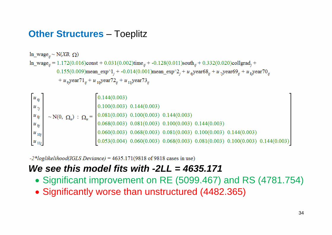
Other Structures – Toeplitz This makes elements of the covariance matrix constant down the diagonals
*
+
This is fairly easy to fit in MLwiN as it can be specified using linear constraints on our fully unstructured model (p.27) o Will fit if you have an AR(1) structure BUT does not
assume the inter-relationships that would exist down the columns…

33
Other Structures – Toeplitz
34
Other Structures – Toeplitz
We see this model fits with -2LL = 4635.171
Significant improvement on RE (5099.467) and RS (4781.754)
Significantly worse than unstructured (4482.365)

35
Just to Finish
Using random slopes with time (as a continuous variable) allows for more complex residual correlations o Can be difficult to interpret in terms of a correlation
structure o Intuitive interpretation with a unique ‘growth curve’ for
each individual
Using random structure on time dummies allows us to be completely unstructured o Can impose linear constraints on the parameters of the
covariance matrix o Can use time dummies in the X as well to get a totally
flexible shape for the growth curve over time

36
SESSION THREE Improving the fixed part of the model

37
Content of Session
The ‘within’ and ‘between’ models
A strong assumption behind random effects
Using contextual effects to get at the within effect
Other extensions o Extra levels o Cross-level interactions

38
Within and Between Effects Let’s go back to a simple random effects model with a single continuous x
We can also define a model for the between (school) effects as
where under expectation uj and vj are the same random error as the eij’s have expected mean zero in the group The difference gives the model for the within (school) effects
39
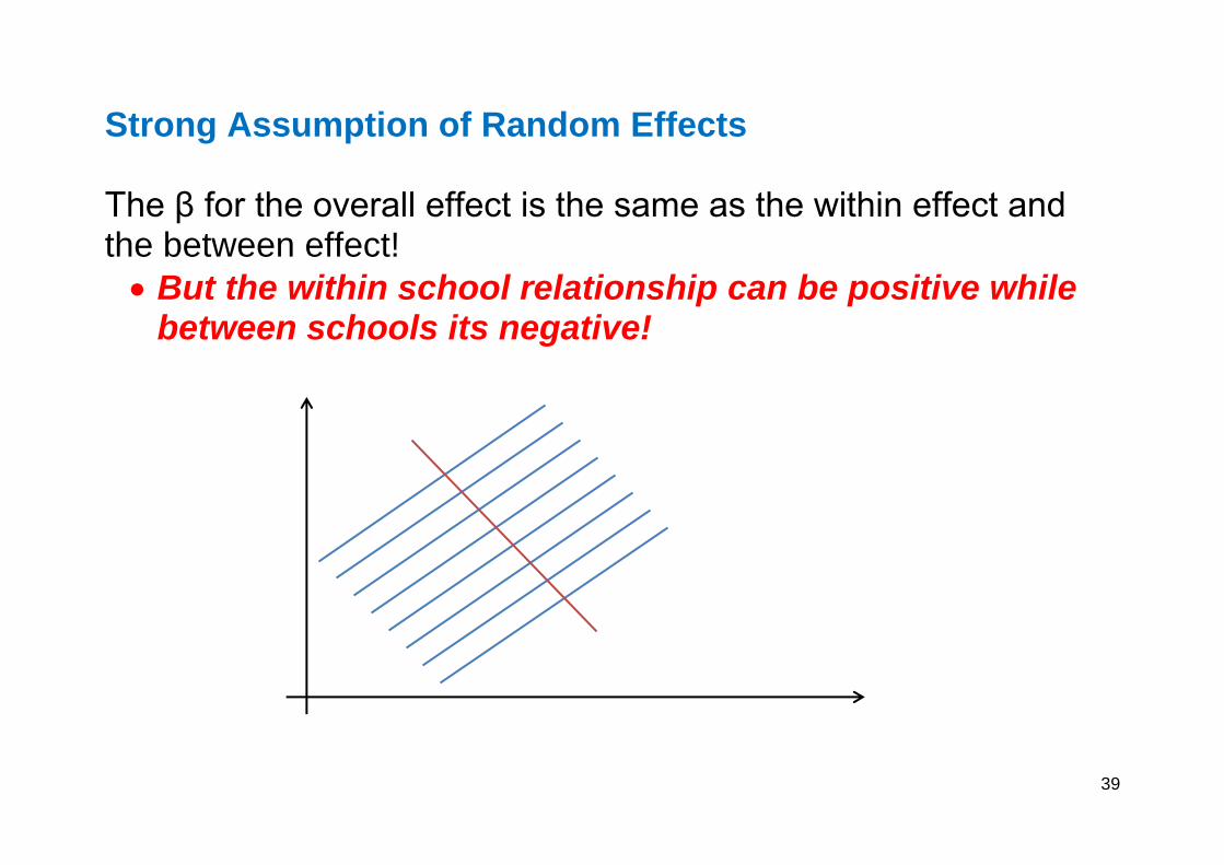
Strong Assumption of Random Effects The β for the overall effect is the same as the within effect and the between effect!
But the within school relationship can be positive while between schools its negative!

40
Strong Assumption of Random Effects This is what economists often worry about!
If I am trying to evaluate impact (a change within each individual) then I want a good estimate of the within effect… o I do not want it to be biased by mixing-up between and
within effects with the random effect Hausmann specification test is used by STATA to test whether the β’s can be assumed the same
We can adjust our model to bring in the group mean as a contextual effect (and centre the original x) o Rabe-Hesketh, S. and Skrondal, A. (2005)
( )

41
Simple Example (with the NLS data) We want to evaluate the impact of moving to the South of the US on wages
South in the data is a time-varying covariate…
A move to the south reduces loge(wages) by 0.155; a 15%
drop in wages

42
Simple Example (with the NLS data) Is it that simple?
Surely we would expect time in the South to impact o Different ‘growth curve’ on wages in the South…
No evidence to support a significant interaction…
o Just a level shift IMPACT…

43
Simple Example (with the NLS data) What about our strong assumption behind the random effects model?
Are we really getting the true within effect here of moving to the South?

44
Simple Example (with the NLS data)
This parameterisation is a significantly better fit and both β’s strongly significant o Clear evidence that the between and within effects are
NOT the same…
Suggests the direct impact of a move is about a 6% drop in wages
Also suggests that the proportion of time spent in the South impacts significantly on the overall level of an individual’s wages

45
Simple Example (with the NLS data)
The effects are still there when we bring in our additional controls…
Still fits significantly better than the standard random
effects model (p.11)

46
Simple Example (with the NLS data)
What about if we extend our correlation structure?
Proportion of time in the South impacts on wages but not the
movement (needs a bit more thought)…

47
Further Extensions – extra levels By fitting our repeated measures models within the multilevel framework we can account for extra clustering
We can relax the assumption that individuals are independent…
Work by a recent PhD student at Southampton has been exploring these models in the context of the Brazilian Labour Force Survey o Rotation panel survey with area clustering…

48
Further Extensions – cross level interactions By fitting our repeated measures models within the multilevel framework we can allow the impact of time to change for different individual level (time-constant) characteristics
Different growth curve for college grads? NO

49
Further Extensions – cross level interactions
Different South Effect for college grads? NO
You might want to explore South with Race…

50
Just to Finish
If you are interested in the direct impact of a change then we need to be careful… o Between and within effects can get messed-up with simple
random effects
Might want to set the data so that there is a variable Move_South that just takes the value 1 the year the move south takes place and is zero otherwise o Move_North would pick-up a move from the South o South picks-up living in the South
Now the β for South will tell us if wages are generally lower in the South o The β’s on the Move_South and Move_North will try and
measure the immediate impact of the change on wages…

51
SESSION FOUR Some alternative approaches

52
Content of Session
Fixed effects
GEE
Other frameworks…

53
Basic Repeated Measures Model This is the basic model structure we have been using for the past two days…
ui represents some residual unobserved effect that individual i
has on the outcome y o It also generates a correlation structure for the
observations
In the random effects situation we assume the ui’s are drawn from some distribution for the population
o So a sample can estimate the population parameter
capturing the residual correlation that exists within individuals in the population

54
Basic Repeated Measures Model – fixed effects approach Suppose I’m only interested in the ‘within effects’
Time-constant effects (including ui) are just a nuisance to me… o Treat them as fixed and then difference them out
o Just like adding a dummy for each individual BUT you don’t need all the parameters Computer drops one observation per individual to
account for estimating the means Classic approach in econometrics (Wooldridge, 2010) to handle panel data
Very easy to fit in STATA…

55
Basic Repeated Measures Model – general estimating equations (GEE) approach
We still have the same model
BUT
We are worried that the correlation structure is more complex than say our simple random effects… o The correlation structure is a nuisance getting in the way
of us estimating…
Need an approach to get good estimates of the fixed parameters in the model o While recognising the existence of complex correlations…

56
General Estimating Equations (xtgee in STATA) For full details see Liang and Zeger (1986) although there is a basic description in Diggle, Liang, and Zeger (1994)
Basic Idea The correlation structure is a nuisance parameter. However, if we specify a working correlation structure that is sensible we can get efficient estimates of the β’s (with robust standard errors) and therefore estimate the ‘marginal’ model for the population.
We iterate between a moments estimator for the correlation structure and an efficient estimator for the β’s
We can then use a marginal model to contrast sub-populations in the data BUT not necessarily to talk about individuals (unless the model follows a Gaussian distribution).

57
General Estimating Equations This leads to a very flexible estimation strategy that can be applied to linear and non-linear data with a whole class of within group/individual correlation structures.
In fact we do not even need to get the correlation structure correct as long as we use robust methods to estimate the standard errors of the β’s. o However, getting a ‘good’ approximation will lead to more
efficient estimation of the β’s.
58
Alternative Framework – Structural Equation Modelling Not my area at all BUT it is an alternative way of handling the ui term
This is an unobserved effect, which we must put some structure on…
GLaMM (Generalised Latent Mixed Models) This is work by Rabe-Hesketh, Skrondal (and others) that gives a framework in which you can fit either a multilevel approach or a structural equation approach
Just depends on the assumptions you impose on the latent structure o Steele (2008) gives a good review of this...

59
Extra References Berrington, A., Smith, P. W. F. and Sturgis, P. (2006) An overview of methods for the analysis of panel data. ESRC National Centre for Research Methods Briefing Paper. Griffiths P., Brown J. and Smith P. W. F. (2004) A comparison of univariate and multivariate multilevel models for repeated measures using uptake of antenatal care in Uttar Pradesh. JRSS(A), 167, pp. 597-611. Steele, F. (2008) Multilevel Models for Longitudinal Data. JRSS(A), 171, pp. 5-19. Singer, J. and Willett J. (2003) Applied Longitudinal Data Analysis: Modelling change and event occurrence. New York: Oxford University Press.