introduction to network modeling using exponential random

HAL Id: hal-01284994https://hal.archives-ouvertes.fr/hal-01284994v2

Preprint submitted on 17 Oct 2017

HAL is a multi-disciplinary open accessarchive for the deposit and dissemination of sci-entific research documents, whether they are pub-lished or not. The documents may come fromteaching and research institutions in France orabroad, or from public or private research centers.

L’archive ouverte pluridisciplinaire HAL, estdestinée au dépôt et à la diffusion de documentsscientifiques de niveau recherche, publiés ou non,émanant des établissements d’enseignement et derecherche français ou étrangers, des laboratoirespublics ou privés.

Copyright

Introduction to network modeling using ExponentialRandom Graph models (ERGM)

Johannes van der Pol

To cite this version:Johannes van der Pol. Introduction to network modeling using Exponential Random Graph models(ERGM). 2017. �hal-01284994v2�

https://hal.archives-ouvertes.fr/hal-01284994v2

https://hal.archives-ouvertes.fr

Introduction to network modeling usingExponential Random Graph models (ERGM):

theory and an application using R-project

Johannes van der Pol

Gretha UMR-CNRS 5113, university of Bordeaux.Avenue Léon Duguit, 33608 Pessac.

Abstract

Exponential Family Random Graph Models (ERGM) are increasingly usedin the study of social networks. These models are build to explain the globalstructure of a network while allowing inference on tie prediction on a micro level.The number of papers within economics is however limited. Possible applicationsfor economics are however abundant. The aim of this document is to provide anexplanation of the basic mechanics behind the models and provide a sample code(using R and the packages statnet and ergm) to operationalize and interpret resultsand analyse goodness of fit. After reading this paper the reader should be able tostart their own analysis.

Introduction

Networks are representations of relational data. Nodes represent entities while thelinks connecting them represent any form of interaction or connection between theentities. A large diversity of networks exists ranging from networks of social contactsbetween individuals to inventor networks, collaboration networks, financial networksand so on. These networks attract the interest of researchers who want to explain thestructure of these networks. In other words, the would like to know why certain agentsare central in a network and why other are at the periphery, why some networks aredensely interconnected and why others are sparse. In essence, we want to know whyfirms a is connected to firm b, or what it the probability that firm a will connect tofirm c and how does this impact the overall structure of the network. This allows usto identify if technological proximity between firms has a significant impact on thechoice of collaborator between firms and if this strategy has a significant impact on thestructure of the network.

Financial support from IdEx Bordeaux and valuable comments and suggestions from Murat Yildizogluare gratefully acknowledged.

1

The motivations for link creation cannot be observed directly from a visual representa-tion of interactions, nor are they clear from glimpsing at a database containing relationaldata. In order to identify the motivations for entities to create links and identify theglobal network structure, a more in-depth analysis is required.Methods such as, Interpretive Structural Modeling, Total Interpretive Structural Model-ing, and Graph Theory Matrix allow for an analysis of the interactions between variablesbut do not allow to for conclusions on the structure of the networks we aim at analysing.In other words, the methods allow for identifying a correlation between technologicalproximity and social proximity but do not explain the structure of the network thatallows this conclusion. Econometric analysis could shed more light on the motivationsbehind an observed link through logistic regressions. The probability of a link could beexplained by a number of variables. There is one important limitation to this method.Due to the hypothesis of independence of the observations the probability of a linkbetween two nodes can never be explained by the presence of another link inside the net-work. It is feasible that a link between two nodes exists only because of the presence ofother links in the network. Take for instance the idea that John and Mary are connectedsolely because they have a common contact: Paul. Methods such as Block-modelscannot account for the impact of the structure of the network on the probability of a link.ERGM models are modified logistic regressions that allow for the probability of a linkto depend upon the presence of other links inside the network (amongst other variables).ERGMs are able to take into account directed interactions as well as weighted interac-tions between nodes. The latter is an important point, since it allows an analysis beyonda simple binary relation between nodes approaching the idea of fuzzy logic.An ERGM identifies the probability distribution of a network so that it can generate largesamples of networks. The samples are then used to infer on the odds of a particular linkinside a network. Applications for this method are numerous in many fields of researchas shown by the increasing trend in the number of publications using ERGM models(see figure 1). In economics the number of published papers appears to be relatively

0

20

40

1995 2000 2005 2010 2015Year

Num

ber

of p

ublic

atio

n

Evolution of the number of ERGM publications

Figure 1: Evolution of the number of publications involving ERG models for alldisciplines (statistics included) (source: Scopus)

2

low when compared to the other social sciences. Only 19 published papers could befound in the Scopus database (and even less in the web of science database). The topicsare however quite diverse: knowledge sharing in organizations (Caimo, Lomi, 2015),GDP targeting (Belongia, Ireland, 2014), alliance networks (Cranmer et al., 2012; Lomi,Pallotti, 2012; Lomi, Fonti, 2012; Broekel, Hartog, 2013) and geographic proximity(Ter Wal, 2013).Since ERGMs allow for hypothesis testing, they can be put into use rather quicklywithin existing theoretical frameworks adding the possibility to analyse relational datain addition to normal data.The growing interest, and development of a theory of economic networks, providesa fertile ground for the use of ERGM models from the geography of innovation toventure capital investments. The aim of this paper is to provide an overview of the basicstatistical theory behind ERGM models, which will be dealt with in the first section.Section 2 discusses the concept of dependence and the explanatory variables that can beincluded in the models. Section 3 discusses estimation methods while section 4 providesthe R scripts and the interpretation of an example using data for the French aerospacesector alliance network.

1 Theory

1.1 The canonical form of ERGM models

i

jk

Figure 2: Network G

The aim of an ERGM is to identify the processes that influence link creation. Theresearcher includes variables in the model that are hypothesised to explain the observednetwork, the ERGM will provide information relative to the statistical significance ofthe included variable much like a standard linear regression.It is useful at this point to explain that sub-structures of a network can (and are pre-dominantly) used as explanatory variables. Substructures are small graphs containedinside the network. Examples can be found in figure 2. The presence of some of thesestructures reflects certain link creation phenomena. A random network, i.e a networkin which links are created at random, show a low number of triangles. A triangle is aninterconnection of three nodes, the smallest possible complete subgraph. The presenceof triangles in an empiric network bares witness that there is a process that generatestriangles that is not the result of random link creation e.g, a tendency to create a linkbetween common friends. A network with a small number of large stars and a largenumber of small stars can be the results of having a small number of very popularnodes. This is found in citation networks as well as lexicographical networks. Includingsub-structures allows the modeling of certain processes as would any other variable.

3

In an ERGM we can find two types of explanatory variables: structural and node oredge-level variables. The latter come from other data sources and can be for exampleage, size of a firm, proximity, gender and so forth. The structural variables can containindicators such as triadic closure, degree distribution and subgraphs.

1.2 The odds of a linkWith this in mind the probability that one would observe a link between any two nodes iand j in a given network is proportional to a given set of explanatory variables:

p(Gij = 1) = θ1 ·X1 + θ2 ·X2 + . . .+ θn ·Xn (1)

We note G a graph and ij the focal nodes. Gij = 1 means that a link exists betweennodes i and j in graph G, Gij = 0 implies the absence of a link between nodes i and j1.θ is a vector of parameters and X a vector containing the variables.Equation 1 gives us the probability of a single link in graph G. Since nothing guaranteesthat the probability stays within [0, 1] the equation needs to be somewhat adjusted. Westart by transforming the probability into an odds ratio:

odds(Gij = 1) =p(Gij = 1)

1− p(Gij = 1)=p(Gij = 1)

p(Gij = 0)(2)

Now, in equation 2 we notice that the odds of a link tend towards zero when theprobability of a link tends towards one, while tending towards −∞ when the probabil-ity tends towards zero. A final modification is required to ensure that the probabilityremains between the bounds of 0 and 1, this is accomplished using the natural logarithm:

log(odds(Gij = 1)) = logit(p(Gij = 1)) = log

(p(Gij = 1)

p(Gij = 0)

)(3)

The probability is now bounded by 0 and 1. If we suppose that the probability of alink is explained by a vector of n variables accompanied by their respective parameters(θ1 . . . θn) then we can write:

logit(p(Gij = 1)) = θ ·X (4)

So in our example we have:

logit(p(Gij = 1)) = θ1 ·X1 + . . . θn ·Xn (5)p(Gij = 1) = exp{θ1 ·X1 + . . . θn ·Xn} (6)

1the values 0 and 1 refer to values found in an adjacency matrix, 1 indicating the presence of a link, 0 theabsence

4

This gives us the logit which supplies the marginal probability of a tie betweennodes i and j. Using these equations the probabilty of a tie between i and j wouldbe independant from the probability between i and k. Indeed, a logistic regressionworks under the hypothesis of independence of observations. In the case of networksobservations are not independent. For instance, common friends tend to connect morein social networks, common collaborators have a higher tendency towards collaboration.A model that aims at explaining a network structure should be able to include these tieformation processes.We hence modify the initial equations to include the network structure as observedbefore the link. This modification is introduced by Strauss, Ikeda (1990). We note Gc

ij

the network without link ij:

odds(Gij = 1) =p(Gij = 1|Gc

ij)

1− p(Gij = 1|Gcij)

=p(Gij = 1|Gc

ij)

p(Gij = 0|Gcij)

(7)

In equation 7 the odds of a link between nodes i and j now depends on the structure ofthe network before a link between i and j is created (noted by |Gc

ij). The probabilitiesare now conditional.We discussed previously that some of the variables in the model can be subgraphs.The manner in which these are included in the model is simply by the count of thesesub-structures. In other words, the value of the variable triangles is the number oftriangles in the network. The same is true for stars, circuits and shared partners. Thishas as a consequence that the counts of these variables are not the same when a linkbetween two nodes is present or absent. For instance the number of edges changes byone. This means that we need to differentiate between the value of the variables when alink is present and when it is absent. We hence note the vector of variables v(G+

ij) whena link between i and j is added (hence the ”+”) and v(G−

ij) when the link is absent. Byincluding this differentiation we can rewrite equation 7 using the result in equation 6:

odds(Gij = 1) =p(Gij = 1|Gc

ij)

p(Gij = 0|Gcij)

=exp{θ′ · v(G+

ij)}exp{θ′ · v(G−

ij)}(8)

Where v(G+ij represents the vector of variables in the network with the link between

i and j present and v(G−ij the vector of variables with no link between i and j.

With some basic algebra we can develop the previous equation a bit further:

exp{θ′ · v(G+ij)}

exp{θ′ · v(G−ij)}

= exp{θ′ · v(G+ij)} · exp{−θ

′ · v(G−ij)} (9)

= exp{θ′(v(G+ij − v(G−

ij)} (10)

When developing the vector of variables we have:

5

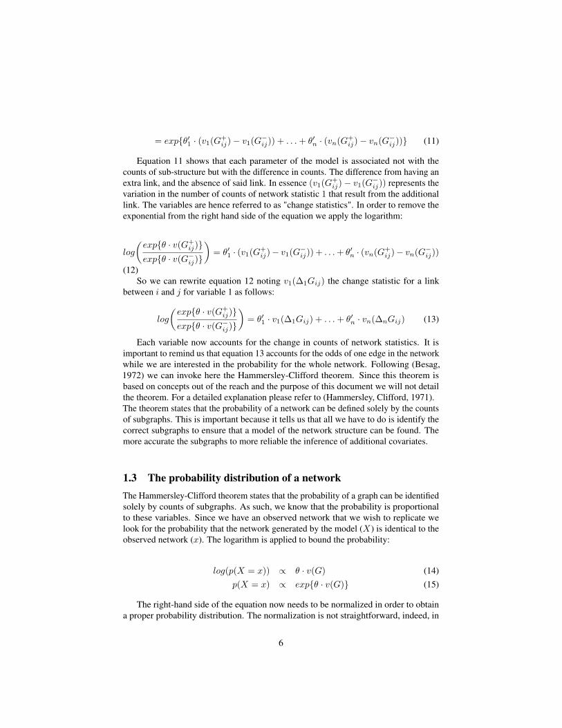
= exp{θ′1 · (v1(G+ij)− v1(G

−ij)) + . . .+ θ′n · (vn(G+

ij)− vn(G−ij))} (11)

Equation 11 shows that each parameter of the model is associated not with thecounts of sub-structure but with the difference in counts. The difference from having anextra link, and the absence of said link. In essence (v1(G

+ij)− v1(G

−ij)) represents the

variation in the number of counts of network statistic 1 that result from the additionallink. The variables are hence referred to as "change statistics". In order to remove theexponential from the right hand side of the equation we apply the logarithm:

log

(exp{θ · v(G+

ij)}exp{θ · v(G−

ij)}

)= θ′1 · (v1(G+

ij)− v1(G−ij)) + . . .+ θ′n · (vn(G+

ij)− vn(G−ij))

(12)So we can rewrite equation 12 noting v1(∆1Gij) the change statistic for a link

between i and j for variable 1 as follows:

log

(exp{θ · v(G+

ij)}exp{θ · v(G−

ij)}

)= θ′1 · v1(∆1Gij) + . . .+ θ′n · vn(∆nGij) (13)

Each variable now accounts for the change in counts of network statistics. It isimportant to remind us that equation 13 accounts for the odds of one edge in the networkwhile we are interested in the probability for the whole network. Following (Besag,1972) we can invoke here the Hammersley-Clifford theorem. Since this theorem isbased on concepts out of the reach and the purpose of this document we will not detailthe theorem. For a detailed explanation please refer to (Hammersley, Clifford, 1971).The theorem states that the probability of a network can be defined solely by the countsof subgraphs. This is important because it tells us that all we have to do is identify thecorrect subgraphs to ensure that a model of the network structure can be found. Themore accurate the subgraphs to more reliable the inference of additional covariates.

1.3 The probability distribution of a networkThe Hammersley-Clifford theorem states that the probability of a graph can be identifiedsolely by counts of subgraphs. As such, we know that the probability is proportionalto these variables. Since we have an observed network that we wish to replicate welook for the probability that the network generated by the model (X) is identical to theobserved network (x). The logarithm is applied to bound the probability:

log(p(X = x)) ∝ θ · v(G) (14)p(X = x) ∝ exp{θ · v(G)} (15)

The right-hand side of the equation now needs to be normalized in order to obtaina proper probability distribution. The normalization is not straightforward, indeed, in

6

order to normalize the probability of a network one needs to normalize by all possiblenetworks with the same number of nodes:

p(X = x) =exp{θ · v(G)}∑

y∈Y exp{θ · v(G)}(16)

With y a possible network structure in the set of all possible networks Y . The nu-merator is normalized by the sum of the parameters over all possible network structures.Note that this number is large. For a network with n nodes the number of possiblegraphs is 2

n(n−1)2 . So even for a graph with 10 nodes there are 35184372088832 possi-

ble graphs. The major problem to overcome with ERGMs is exactly this normalizingconstant.

With some simple algebra we find a general form for this model. Using θ as a vectorof parameters and v(G) a vector of variables for network G:

p(X = x) =exp{θ · v(G)}

exp{log(∑

y∈Y exp{θ · v(G)}})(17)

p(X = x) =1

ψ(θ)· exp{θ · v(G)} = exp{θ · v(G)− ψ(θ)} (18)

Equation 18 is the most general and commonly used form of the model (Lusheret al., 2012). Equation 18 also gives the canonical form of an ERGM model. Sincethe density of the random variable (the network structure) has the particular form inequation 18 it is referred to as an exponential family. In addition, since the structuresare represented by a random variable, they are random graphs.

Putting both elements together and this results in an Exponential Family RandomGraph. Since ERGM is easier to pronounce than EFRGM, the models are referred to asERGM2.

The canonical form gives the equation we wish to estimate. However, before wetackle the question of estimation we need to explore in more detail the variables that wewould want to include in the model. We have stated previously that counts of subgraphscan be used as explanatory variables. The following section will explain which particularsubgraphs are to be included in a model.

2 The dependence assumptionThe previous section has shown that ERGMs are capable of providing conditionalprobabilities for links. This dependence assumption is important because it allowsthe researcher to study different phenomena that rule the formation of networks. Thissection will show how the hypothesis of dependence of links is connected to the choiceof subgraphs that may be included in an analysis.

2This type of model is also referred to as the P ∗ family of models (Anderson et al., 1999; Lusher et al.,2012).

7

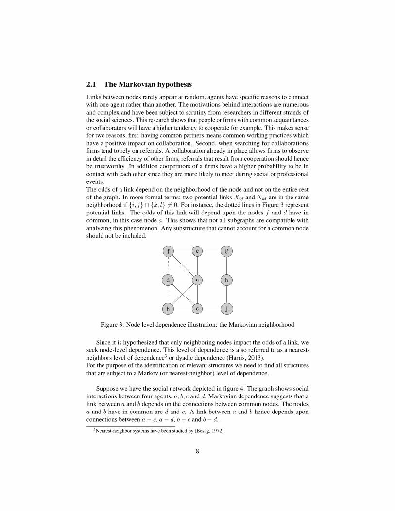
2.1 The Markovian hypothesisLinks between nodes rarely appear at random, agents have specific reasons to connectwith one agent rather than another. The motivations behind interactions are numerousand complex and have been subject to scrutiny from researchers in different strands ofthe social sciences. This research shows that people or firms with common acquaintancesor collaborators will have a higher tendency to cooperate for example. This makes sensefor two reasons, first, having common partners means common working practices whichhave a positive impact on collaboration. Second, when searching for collaborationsfirms tend to rely on referrals. A collaboration already in place allows firms to observein detail the efficiency of other firms, referrals that result from cooperation should hencebe trustworthy. In addition cooperators of a firms have a higher probability to be incontact with each other since they are more likely to meet during social or professionalevents.The odds of a link depend on the neighborhood of the node and not on the entire restof the graph. In more formal terms: two potential links Xij and Xkl are in the sameneighborhood if {i, j} ∩ {k, l} 6= 0. For instance, the dotted lines in Figure 3 representpotential links. The odds of this link will depend upon the nodes f and d have incommon, in this case node a. This shows that not all subgraphs are compatible withanalyzing this phenomenon. Any substructure that cannot account for a common nodeshould not be included.

a b

c

d

ef g

h j

Figure 3: Node level dependence illustration: the Markovian neighborhood

Since it is hypothesized that only neighboring nodes impact the odds of a link, weseek node-level dependence. This level of dependence is also referred to as a nearest-neighbors level of dependence3 or dyadic dependence (Harris, 2013).For the purpose of the identification of relevant structures we need to find all structuresthat are subject to a Markov (or nearest-neighbor) level of dependence.

Suppose we have the social network depicted in figure 4. The graph shows socialinteractions between four agents, a, b, c and d. Markovian dependence suggests that alink between a and b depends on the connections between common nodes. The nodesa and b have in common are d and c. A link between a and b hence depends uponconnections between a− c, a− d, b− c and b− d.

3Nearest-neighbor systems have been studied by (Besag, 1972).

8

a

b

cd

Figure 4: Markov graph

ad

ab ac

bd bc

dc

Figure 5: Dependence graph

ad

ab ac

bd bc

dc

Figure 6: Dependence graph andconfiguration identification

ad ab

a b

d

Figure 7: 2-star identification in thedependence graph

When one identifies all the possible dependencies one can generate a dependence graph.The dependence graph for the complete Markov graph in our example can be found infigure 6. In red we find the dependence links for link a− b, it show the links on whicha− b depends.From this graph one can identify the substructures that comply with Markovian de-pendence. All subgraphs in the dependence graph can be included in a model to addMarkovian dependence. For example, the dotted line between ab and ad represents a2-star centered on agent a (figure 7).

Using the same method as for the 2-star one can also identify a triangle betweenthe three agents on the links bd, bc and dc. The Markov model hence includes threeconfigurations: edges, 2-stars and triangles. With the inclusion of these configurationsthe Markovian model takes the form:In more complex graphs one could also identify 3-stars, 4-stars etc.It should be obvious here that the number of distinct 2-stars is large and it is nearimpossible to add a parameter for each distinct 2-star in the dependence graph. To

9

reduce the number of variables a hypothesis is made that each type of configurationhas the same probability of appearance, this allows for the inclusion of one parameterper substructure. In the case of Markov dependence the ERGM model would have thefollowing form:

p(x = X|θ) = 1

ψ(θ)exp{θE ·vE(x)+θS2 ·vS2 + . . . +θSn−1 ·vSn−1 +θ∆ ·v∆} (19)

Where θE is the parameter for the number of edges, θS2 the parameter for thenumber of 2-stars and θ∆ the parameter for the number of triangles. Note here that themodel does not include simultaneously a 1-star and an edge parameter since they wouldbe the same variable. With this model one is able to study if common nodes have apositive impact on the odds of link creation.In addition the combination of the 2-star parameter and the triangle parameter accountfor triadic closure effects. In other words, are triangles created because 3 nodes areconnected at the same time, or are triangles formed by the closing of a 2-star.

Of course, Markovian dependence is only one of the possible levels of dependence.One can imagine higher levels of dependence, or even any level of dependence tobe empirically relevant. One could suggest that firms evolving on the periphery ofa network to have a higher probability to connect with firms in the center of the net-work than between them. The previous model was hence extended by Wasserman,Pattison (1996) to allow for a general level of conditional dependence giving the re-searcher a total liberty in the theories to test. Whatever the level of dependence chosen,the dependence graph gives the substructure that may be included (Frank, Strauss, 1986).

2.1.1 Higher levels of dependence

It is possible to assume that the Markovian level of dependence is not adequate or doesnot capture the full complexity of mechanisms of link creation. Links can be dependentwithout there being a common node involved. For instance, consider a case in whichpeople work on the same floor in a company. The probability of a social link doesnot depend upon a common node but simply on the fact that they are geographicallyclose, belong to the same community or have common cultural aspects (White, 1992).In order to be able to model more complex aspects of social interactions and indeedeven strategic interactions, one needs to be able to account for more structural aspectsthan stars and triangles (however potent in explanatory power these might be). Thelatter implies that the links are only dependent on each-other if nodes are part of a sameneighborhood (neighborhood takes a broad definition here, it can be social, geographicalor cultural). Due to the inclusion of general dependence the model is transformed totake the form:

10

p(x = X) =1

ψ(θ)exp{

∑A∈M

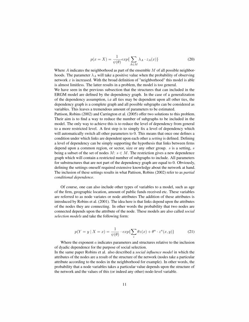
λA · zA(x)} (20)

Where A indicates the neighborhood as part of the ensemble M of all possible neighbor-hoods. The parameter λA will take a positive value when the probability of observingnetwork x is increased. With the broad definition of "neighborhood" this model is ableis almost limitless. The latter results in a problem, the model is too general.We have seen in the previous subsection that the structures that can included in theERGM model are defined by the dependency graph. In the case of a generalizationof the dependency assumption, i.e all ties may be dependent upon all other ties, thedependency graph is a complete graph and all possible subgraphs can be considered asvariables. This leaves a tremendous amount of parameters to be estimated.Pattison, Robins (2002) and Carrington et al. (2005) offer two solutions to this problem.Their aim is to find a way to reduce the number of subgraphs to be included in themodel. The only way to achieve this is to reduce the level of dependency from generalto a more restricted level. A first step is to simply fix a level of dependency whichwill automatically switch all other parameters to 0. This means that once one defines acondition under which links are dependent upon each other a setting is defined. Defininga level of dependency can be simply supporting the hypothesis that links between firmsdepend upon a common region, or sector, size or any other group. s is a setting, sbeing a subset of the set of nodes M : s ∈M . The restriction gives a new dependencegraph which will contain a restricted number of subgraphs to include. All parametersfor substructures that are not part of the dependency graph are equal to 0. Obviously,defining the settings oneself required extensive knowledge about the network at hand.The inclusion of these settings results in what Pattison, Robins (2002) refer to as partialconditional dependence.

Of course, one can also include other types of variables to a model, such as ageof the firm, geographic location, amount of public funds received etc. These variablesare referred to as node variates or node attributes The addition of these attributes isintroduced by Robins et al. (2001). The idea here is that links depend upon the attributesof the nodes they are connecting. In other words the probability that two nodes areconnected depends upon the attribute of the node. These models are also called socialselection models and take the following form:

p(Y = y | X = x) =1

ψ(θ)· exp{

∑i

θz(x) + θa · za(x, y)} (21)

Where the exponent a indicates parameters and structures relative to the inclusionof dyadic dependence for the purpose of social selection.In the same paper Robins et al. also described a social influence model in which theattributes of the nodes are a result of the structure of the network (nodes take a particularattribute according to the nodes in the neighborhood for example). In other words, theprobability that a node variables takes a particular value depends upon the structure ofthe network and the values of this (or indeed any other) node-level variable.

11

We hence need to add a node variables to the model. Suppose we note Yi the value of anode variable for node i. This variable can be anything from a geographic region to theamount of public investment received by firms to the number of publications or patents.When this variable is included in the ERGM the model is written:

p(Y = y | X = x) =1

ψ(θi)· exp{

∑i

θz(y, x)} (22)

Just as it is possible to put values on nodes it is also possible to values on dyads.The question then is to know if the value of the dyad increases the probability of nodesbeing connected. Think of situations where we would like to know if the amount ofinvestment between firms is related to cooperation or if technological proximity betweenfirms induces collaboration. Note here that the difference between dyadic covariatesand actor attributes resides in the value on the link between two nodes. In the case ofproximity is refers to the proximity of both firms, it is hence not a firm-level variable.The value only makes sense when we consider firms two-by-two.

All the extensions made to the ERGM framework allow researchers to answer a largevariety of questions about social and economic processes. Many other extensions whichare beyond the scope of this document, but worth noting, are multivariate relations innetworks (Pattison, Wasserman, 1999) and dynamic networks in which new ties dependupon the structure of the network at time t− 1. It is also possible to model multivariatenetworks using ERGM. The idea is then that each link can exist in different matrixes,each corresponding to a different type of link (social, work, geography etc.). Thisextension allows researchers to study interplay between different networks and howeach network is affected by the other networks.

Before looking at estimation methods for ERGM models one problem needs to beaddressed: the degeneracy problem.

2.2 Solving degeneracy: Curved ERGMsERGM models are prone to degeneracy issues. When estimating the model the changestatistics can behave in such a way that the large majority of the probability distributionis placed on either an empty or a full graph. As we will discuss in more detail a bit later,a simulation is performed to identify the probability distribution of a graph. This is doneon a step by step basis, starting with an empty network and adding links one by oneuntil a maximum likelihood is achieved. This probability distribution is a function of thechange statistics and is thus impacted by the change in log-odds for an additional tie (fora given effect). In other words if an additional edge would create two new 2-stars, thenthe log-odds of observing that tie would increase by two multiplied by the parameterof the 2-star variable. A random graph model is considered stable if small changes inthe parameter values result in small changes in the probabilistic structure of the model(Handcock et al., 2003). When a new edge is added to the graph this not only increasesthe number of edges but might also increase the number of other sub-configurations

12

that might be included in the model. The parameters of the model control the numberof sub-graphs of a particular type that are expected in the graph. For instance a 2-starmight be transformed into a triangle by the addition of an edge which also adds two2-stars. A 2-star can become at 3-star and so on. This cascading effect will result in thesimulation procedure jumping over the MLE and converge to a full graph. Lusher et al.(2012) [chapter 6] show that, in the case of the Markov (or triad model), the numberof expected triangles increases as the parameter for triangles increases. They highlighta phase transition for certain values of the parameter where the number of expectedtriangles increases more than exponentially. This transition explain that the probabilitydensity distribution has high weights either on a (close to) empty graph or on a completegraph4. This problem is increasingly present as the number of nodes increases. Thelarger the network the higher the number of substructures one can have.In order to avoid the model to put too much weight on the full graphs, Snijders et al.(2006) propose to add several variables based on their concept of partial conditionaldependence. The idea is to include a weighted degree distribution to the model, giving ahigh weight to low density while decreasing the weights as the degree increases. Thisreduces the impact of the high density variables responsible for the degeneracy of theinitial model. Mathematically we can then write (using the notations of the initial paper):

u(d)α =

n−1∑k=0

e−αkdk(y) (23)

Where dk(y) is the number of nodes with degree k and α the parameter of theweights. This is referred to as the geometrically weighted degree distribution. Thedegree distribution can also be written as a function of the stars in the network. After all,a degree distribution is nothing more than a distribution of stars. Nodes with a degreeof five are 5-stars, degree two are 2-stars and so forth. We can hence formulate thedistribution as follows:

usλ = S2 −S3

λ+S4

λ2− . . .+ (−1)n−2 · Sn−1

λn−3=

n−1∑k=2

(−1)k · Sk

λk−2(24)

Where Sk is a the number of stars of degree k and lambda the parameter. Thismethod is referred to as Aternating k-stars. The difference between the geometricallyweighted degree distribution and the K-stars is resides in the alternating signs. A largevalue of 3-stars is counterbalanced by a negative value for 4-stars due to the inverse signof the parameter. The addition of the weights ensures that the change in change statisticsstays small. Indeed Snijders et al. (2006) show that the change statistics can be written:

zij = −(1− e−α)(e−α ˜yi+ + e−α ˜yj+) (25)

Where ˜yi+ is the density of firm i when the link between i and j is added. Equation25 shows that the value of the change statistic is reduced by the factor −(1− e−α). This

4In addition, the degeneracy of the model can result in problems with the estimation procedures.

13

factor hence ensures that the change statistics do not take too high values and result ina nested probability distribution. The inclusion of either the alternating k-stars or thegeometrically weighted degrees transform the ERGM model into a Curved ExponentialRandom Graph Model (Efron, 1975).

All that is left to do now is estimate the model.

3 EstimationEstimation allows for the identification of the parameters that maximize the likelihoodof a graph. Since we only have one observation (the observed graph) a set of graphsfrom the same distribution is required. The set of graphs that may be generated by thisprocedure should have the observed graph as a central element to ensure a valid sample.

3.1 Markov Chain Monte CarloIn the first section we identified the general form of an ERGM model (see equation18). The odds of a graph were normalized by the sum of the parameters of all pos-sible graphs. This leaves us with a constant to estimate which is near impossible. Aworkaround has to be found for ERGMs to be useful. A first development by Besag(1975); Strauss, Ikeda (1990) was to estimate the model using pseudo-likelihood estima-tion. The properties of this method are however not clear (Snijders et al., 2006; Robinset al., 2007) we shall hence focus here on more recent methods that are better understood.

A method for estimating the parameters of ERGMs using a sample is developedby Anderson et al. (1999); Snijders (2002); Geyer, Thompson (1992). They estimatethe model by Markov Chain Monte Carlo (MCMC) to find the maximum likelihoodestimates (MLE). The idea is to extract a sample from a distribution that follows equation18 asymptotically, not requiring the direct computation of the normalizing constant.Their paper points out that almost any maximum likelihood can be accomplished by aMCMC.A Markov chain is a sequence of random variables such that the value taken by therandom variable only depends upon the value taken by the previous variable. We canhence consider a network in the form of an adjacency matrix in which each entry isa random variable. By switching the values of these variables to 0 or to 1 (adding orremoving a link from the network) one can generate a sequence of graphs such thateach graph only depends upon the previous graph. This would be a Markov chain. Thehypothesis is then that if the value at step t is drawn from the correct distribution thanso will the value at step t+ 1. Unlike regular Monte-Carlo methods, the observationsthat are sampled are close to each-other since they vary by a single link. However, onewould need a method for selecting which variable should change state in order to getcloser to the MLE, this is done using the Metropolis-Hastings algorithm or the Gibbssampler.

14

3.2 Metropolis-Hastings algorithm and the Gibbs samplerThe Metropolis-Hastings algorithm picks a variable at random and changes it’s state.This results in either a new edge in the network or in the disappearance of an edge. Theprobability of the graph is then computed and only if the probability of the altered graphis higher than the previous one is the new graph retained for the next step. In otherwords the new graph is retained as long as the likelihood is increased:

min{1,pθ(x∗)

pθ(xm−1)} (26)

This decision rule is called the Hastings ratio. The advantage of this ratio is that it doesnot include the normalizing constant ψ(θ).Since the Markov chain starts at 0, a burn-in in needed to remove part of the chain toidentify if the chain has converged or not (the burn-in can be parameterised in mostsoftware).The steps taken by the Metropolis-Hastings algorithm are quite small. These small stepsare implemented in order to avoid overstepping the global optimum which can easilyhappen in the case of larger parameter spaces. Other methods allow for bigger steps andas such converge faster and need a lower burn-in. The risk of larger steps is howeveroverstepping the global optimum and convergence towards other local optima. TheMetropolis-Hastings algorithm may be slower than others but is more precise in it’sestimation.

Some programs use the Gibbs sampler, which is a special case of the Metropolis-hastings algorithm (Hunter, Handcock, 2006). The difference between Gibbs andMetropolis-Hastings resides in the chosen step. In the case of the Gibbs sampler, thestate of each element in the vector of parameters is chosen and updated conditionally onthe state of the other parameters. This means that if this decision rule was implementedin the Metropolis-Hastings algorithm the probability that the change is retained is equalto one. This makes the Gibbs sampler a relatively fast method. This sampling method isused by the different algorithms that are used to estimate ERGM models.Both methods allow for the generation of a sample of graphs that can be used forinference. The sample of graphs is obtained by varying not the parameters but thevariables of the model until it is centered around the observed graph. Now that a sampleof graphs has been found we need to estimate the parameters of the model. Two ofthe most widely used estimation algorithms, the "Stepping" and "Robbins-Monro"algorithm will now be reviewed.

3.3 The "Stepping algorithm"This method introduced by Hummel et al. (2012). It has the advantage of approachingthe MLE directly while "Robbins-Monro" does not. ERGM models are indeed estimatedusing the maximum likelihood method. Starting from the canonical ERGM form wedefine the log likelihood function as:

15

L(θ) = θ · v(G)− log(ψ(θ)) (27)

The problem here is the presence of the normalizing constant which cannot tocomputed. The improvements of this method over the previously one resides in the useof a log-normal approximation. The algorithm proposed here will converge towards thelog-likelihood using a step-by-step method. The sampler used in with this estimationprocedure is the metropolis-hastings sampler discussed previously. Once a sample ofgraphs has been identified the estimation algorithm is launched. Since the normalizingconstant in equation 27 cannot be compute a workaround has to be found. The idea isto give starting parameters (θ0).The log-likelihood ratio can then be written (Hummelet al., 2012):

L(θ)− L(θ0) = (θ − θ0)TV (G)− logEθ0 [exp(θ − θ0)

TV (g)] (28)

Geyer, Thompson (1992) point out that maximizing this ration by the means of asample distribution of graphs generated with θ0 only behaves well when θ is close to θ0.In other words one has to choose the correct starting point for the algorithm to find theMLE. The MLE solves the equation:

Eθ̂v(G) = v(Gobs) (29)

The idea is to suppose that the MLE is not the observed value of the parametersbut some point between the mean value parameterization and the observed value. Aparameter γ defines the steps taken:

ω̂t = γt · v(G) + (1− γt)ω̄ (30)

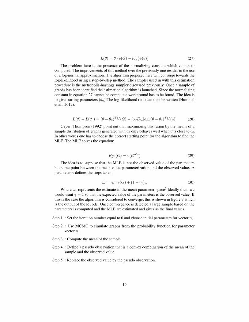
Where ωt represents the estimate in the mean parameter space5.Ideally then, wewould want γ = 1 so that the expected value of the parameters is the observed value. Ifthis is the case the algorithm is considered to converge, this is shown in figure 8 whichis the output of the R code. Once convergence is detected a large sample based on theparameters is computed and the MLE are estimated and gives as the final values.

Step 1 : Set the iteration number equal to 0 and choose initial parameters for vector η0.

Step 2 : Use MCMC to simulate graphs from the probability function for parametervector η0.

Step 3 : Compute the mean of the sample.

Step 4 : Define a pseudo observation that is a convex combination of the mean of thesample and the observed value.

Step 5 : Replace the observed value by the pseudo observation.

16

1 I t e r a t i o n # 1 . T ry in g gamma= 0 . 1 72 I t e r a t i o n # 2 . T ry in g gamma= 0 . 1 43 I t e r a t i o n # 3 . T ry in g gamma= 0 . 1 64 I t e r a t i o n # 4 . T ry in g gamma= 0 . 2 25 I t e r a t i o n # 5 . T ry in g gamma= 0 . 2 56 I t e r a t i o n # 6 . T ry in g gamma= 0 . 3 47 I t e r a t i o n # 7 . T ry in g gamma= 0 . 3 18 I t e r a t i o n # 8 . T ry in g gamma= 0 . 4 69 I t e r a t i o n # 9 . T ry in g gamma= 0 . 7 4

10 I t e r a t i o n # 10 . T ry in g gamma= 0 . 9 711 I t e r a t i o n # 11 . T ry in g gamma= 112 I t e r a t i o n # 12 . T ry in g gamma= 113 Now en d i ng wi th one l a r g e sample f o r MLE.14 E v a l u a t i n g log−l i k e l i h o o d a t t h e e s t i m a t e . Using 20 b r i d g e s : 1 2 3 4 5

6 7 8 9 10 11 12 13 14 15 16 17 18 19 20 .

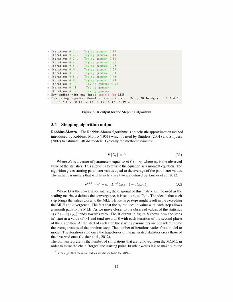
Figure 8: R output for the Stepping algorithm

3.4 Stepping algorithm outputRobbins-Monro The Robbins-Monro algorithme is a stochastic approximation methodintroduced by Robbins, Monro (1951) which is used by Snijders (2001) and Snijders(2002) to estimate ERGM models. Typically the method estimates:

E{Zθ} = 0 (31)

Where Zθ is a vector of parameters equal to u(Y )− u0 where u0 is the observedvalue of the statistics. This allows us to rewrite the equation as a moment equation. Thealgorithm gives starting parameter values equal to the average of the parameter values.The initial parameters that will launch phase two are defined by(Lusher et al., 2012):

θt+1 = θt − at ·D−1(z(xm)− z(xobs)) (32)

Where D is the co-variance matrix, the diagonal of this matrix will be used as thescaling matrix. a defines the convergence, it is set to at =

at−1

2 . The idea is that eachstep brings the values closer to the MLE. Hence large steps might result in the exceedingthe MLE and divergence. The fact that the ar reduces in value with each step allowsa smooth path to the MLE. As we move closer to the observed values of the statisticsz(xm) − z(xobs) tends towards zero. The R output in figure 8 shows how the steps(a) start at a value of 0.1 and tend towards 0 with each iteration of the second phaseof the algorithm. At the start of each step the starting parameters are considered to bethe average values of the previous step. The number of iterations varies from model tomodel. The iterations stop once the trajectories of the generated statistics cross those ofthe observed ones (Lusher et al., 2012).The burn-in represents the number of simulations that are removed from the MCMC inorder to make the chain "forget" the starting point. In other words it is to make sure the

5In the algorithm the initial values are chosen to be the MPLE

17

starting values do not impact the final result.Finally the algorithm checks for convergence using a convergence statistic. Just as in thecase of the stepping algorithm one supposes that the MLE is reached when the distancebetween the observed values and the average of the simulated ones is close to 0. If thereis no convergence than one can relaunch the estimation with as starting parameters theresults of the previous simulation (Lusher et al., 2012).

The largest difference between this method and the stepping method resides in twofactors. First this method approaches an estimate of the MLE and does not evaluate theMLE function directly. Second, the steps are of a higher magnitude and can exceed theMLE if the starting values are close to the MLE. The use of either of the algorithmspurely depends upon the model to be estimated. One algorithm might have betterconvergence in one case while the opposite can be true in another case. Note howeverthat both use the Metropolis-Hastings method for the simulation of the MC.

Now that we have discussed which variables can be included and how to estimatethe parameters we will turn to an application using R.

1 Robbins−Monro a l g o r i t h m wi th t h e t a _0 e q u a l t o :2 edges t r i a n g l e3 −4.676219 1 .4563804 Phase 1 : 13 i t e r a t i o n s ( i n t e r v a l =1024)5 Phase 1 c o m p l e t e ; e s t i m a t e d v a r i a n c e s a r e :6 edges t r i a n g l e7 3676 .692 1175 .3088 Phase 2 , s u b p h a s e 1 : a= 0 . 1 , 9 i t e r a t i o n s ( b u r n i n =16384)9 t h e t a new : −4.66068075119643

10 t h e t a new : 1 .4276892489956811 Phase 2 , s u b p h a s e 2 : a= 0 . 0 5 , 23 i t e r a t i o n s ( b u r n i n =16384)12 t h e t a new : −4.6474090395827313 t h e t a new : 1 .423566924236214 Phase 2 , s u b p h a s e 3 : a= 0 .025 , 58 i t e r a t i o n s ( b u r n i n =16384)15 t h e t a new : −4.6288185640647416 t h e t a new : 1 .4140559396604217 Phase 2 , s u b p h a s e 4 : a= 0 .0125 , 146 i t e r a t i o n s ( b u r n i n =16384)18 t h e t a new : −4.6098509638891419 t h e t a new : 1 .3993281339095420 Phase 3 : 20 i t e r a t i o n s ( i n t e r v a l =1024)21 E v a l u a t i n g log−l i k e l i h o o d a t t h e e s t i m a t e .

Figure 9: R output for the Robbins-Monro algorithm

4 Code R and exampleWe use here different R packages (Hunter et al., 2008a) , (Hunter et al., 2008b; Handcocket al., 2008; Butts, 2008).

The data (and hence the results of the estimations) are from the French aerospacecollaboration network. Using patent data collaborations were identified which resultedin a network. The aim of the study is to understand if technological proximity played a

18

significant role in the structuring of the collaboration network. We hence used a dyadiccovariate called "proximity". The network contains 176 firms.

1 # Imp or t d a t a .2 Network<−r e a d . t a b l e ( "ADJ_MATRIX . csv " , sep =" ; " )

The data used here was already in the form of an adjacency matrix and hence couldbe used directly. It is however also possible to use edgelists. Since the data needs tobe transformed into a network object the network package will be needed. The latter isable to transform edgelists into adjacency matrices.

1 # Imp or t t h e d y a d i c c o v a r i a t e s2 p r o x i m i t y<−r e a d . t a b l e ( " P r o x i m i t y _ m a t r i x . csv " , sep =" ; " )3 p r o x i m i t y . e<−r e a d . t a b l e ( " P r o x i m i t y _ m a t r i x _ exp . csv " , sep =" ; " , dec=" , " )4 c i t a t i o n<−r e a d . t a b l e ( " C i t a t i o n _ m a t r i x . csv " , sep =" ; " )

Since I’m using two measures of proximity I have two matrices and a matrix thatincludes the number of citations between firms. These need to be imported in the samemanner as the network itself.

1 #We now t r a n s f o r m t h e i m p o r t e d d a t a i n t o ne twork o b j e c t s w i th t h epackage ’ network ’

2 Network<−as . m a t r i x ( Network )3 p r o x i m i t y<−as . m a t r i x ( p r o x i m i t y )4 p r o x i m i t y . e<−as . m a t r i x ( p r o x i m i t y . e )5

6 # Trans fo rm t o ne twork f o r m a t7 Network<− as . ne twork ( Network , d i r e c t e d = FALSE)8 p r o x i m i t y<−as . ne twork ( p r o x i m i t y , d i r e c t e d =FALSE)9 exp _ p r o x i m i t y<−as . ne twork ( exp _ p r o x i m i t y , d i r e c t e d =FALSE)

10 c i t a t i o n<−as . ne twork ( c i t a t i o n , d i r e c t e d =TRUE)

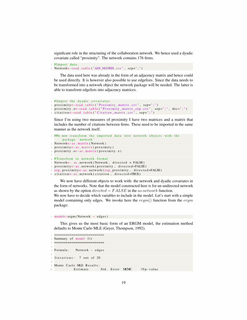
We now have different objects to work with: the network and dyadic covariates inthe form of networks. Note that the model constructed here is for un undirected networkas shown by the option directed = FALSE in the as.network function.We now have to decide which variables to include in the model. Let’s start with a simplemodel containing only edges. We invoke here the ergm() function from the ergmpackage:

1 model<−ergm ( Network ~ edges )

This gives us the most basic form of an ERGM model, the estimation methoddefaults to Monte Carlo MLE (Geyer, Thompson, 1992).

1 ==========================2 Summary of model f i t3 ==========================4

5 Formula : Network ~ edges6

7 I t e r a t i o n s : 7 o u t o f 208

9 Monte C a r l o MLE R e s u l t s :10 E s t i m a t e S td . E r r o r MCMC \%p−v a l u e

19

11 edges −3.85280 0 .05649 0 <1e−04 ∗∗∗12 −−−13 S i g n i f . codes : 0 ’∗∗∗ ’ 0 . 001 ’∗∗ ’ 0 . 0 1 ’∗ ’ 0 . 0 5 ’ . ’ 0 . 1 ’ ’ 114

15 Nul l Deviance : 21349 on 15400 d e g r e e s o f f reedom16 R e s i d u a l Deviance : 3113 on 15399 d e g r e e s o f f reedom17

18 AIC : 3115 BIC : 3122 ( S m a l l e r i s b e t t e r . )

The parameter for the variable edges has an estimated value of -3.8528. This meansthat the probability of two ties connecting is:

p(i→ j) =exp(−3.85)

1− exp(−3.85)= 0.02174241 (33)

Recall equation 11, this equation stated that the variables were change statistics.The parameter should hence be multiplied by the change in the number of subgraphs.In other words, if an additional edge creates three triangles the parameter should bemultiplied by three. Since an additional edge only creates one new edge we do notmultiply. Let’s try the same but with only triangles as explanatory variable.


5 Formula : Network ~ t r i a n g l e s6

7 I t e r a t i o n s : NA8

9 S t e p p i n g MLE R e s u l t s :10 E s t i m a t e S td . E r r o r MCMC \% p−v a l u e11 t r i a n g l e −1.91496 0 .01712 0 <1e−04 ∗∗∗12 −−−13 S i g n i f . codes : 0 ’∗∗∗ ’ 0 . 001 ’∗∗ ’ 0 . 0 1 ’∗ ’ 0 . 0 5 ’ . ’ 0 . 1 ’ ’ 114



The parameter for the variable triangles has an estimated value of -1.9146. Thismeans that the log-odds of two nodes connecting is:

−1.9146 ∗ δ triangles (34)

Where δ triangles gives the change in the number of triangles. Hence the log-oddsdepend upon the number of triangles that will be created by an additional tie:

> If the link creates 1 triangle, the log-odds are 1 * -1.9146. The probability is then0.1284

> If the link creates 2 triangles, the log-odds are 2 * -1.9146. The probability isthen 0.0213

20

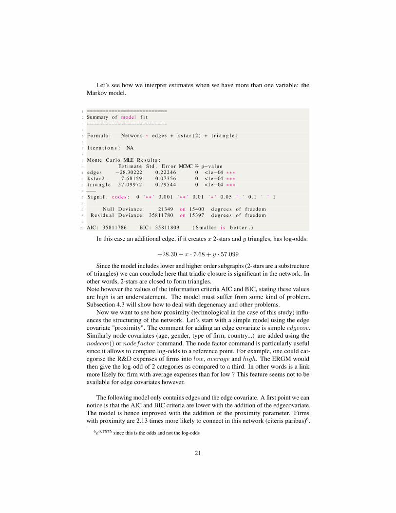
Let’s see how we interpret estimates when we have more than one variable: theMarkov model.


5 Formula : Network ~ edges + k s t a r ( 2 ) + t r i a n g l e s6


9 Monte C a r l o MLE R e s u l t s :10 E s t i m a t e S td . E r r o r MCMC % p−v a l u e11 edges −28.30222 0 .22246 0 <1e−04 ∗∗∗12 k s t a r 2 7 .68159 0 .07356 0 <1e−04 ∗∗∗13 t r i a n g l e 57 .09972 0 .79544 0 <1e−04 ∗∗∗14 −−−15 S i g n i f . codes : 0 ’∗∗ ’ 0 . 001 ’∗∗ ’ 0 . 0 1 ’∗ ’ 0 . 0 5 ’ . ’ 0 . 1 ’ ’ 116



In this case an additional edge, if it creates x 2-stars and y triangles, has log-odds:

−28.30 + x · 7.68 + y · 57.099

Since the model includes lower and higher order subgraphs (2-stars are a substructureof triangles) we can conclude here that triadic closure is significant in the network. Inother words, 2-stars are closed to form triangles.Note however the values of the information criteria AIC and BIC, stating these valuesare high is an understatement. The model must suffer from some kind of problem.Subsection 4.3 will show how to deal with degeneracy and other problems.

Now we want to see how proximity (technological in the case of this study) influ-ences the structuring of the network. Let’s start with a simple model using the edgecovariate "proximity". The comment for adding an edge covariate is simple edgecov.Similarly node covariates (age, gender, type of firm, country...) are added using thenodecov() or nodefactor command. The node factor command is particularly usefulsince it allows to compare log-odds to a reference point. For example, one could cat-egorise the R&D expenses of firms into low, average and high. The ERGM wouldthen give the log-odd of 2 categories as compared to a third. In other words is a linkmore likely for firm with average expenses than for low ? This feature seems not to beavailable for edge covariates however.

The following model only contains edges and the edge covariate. A first point we cannotice is that the AIC and BIC criteria are lower with the addition of the edgecovariate.The model is hence improved with the addition of the proximity parameter. Firmswith proximity are 2.13 times more likely to connect in this network (citeris paribus)6.

6e0.7575 since this is the odds and not the log-odds

21

The probability of an additional edge is then positively impacted by the technologicalproximity. More specifically the average degree of the network is positively impactedby technological proximity.


5 Formula : Network ~ edges + edgecov ( p r o x i m i t y )6


9 Monte C a r l o MLE R e s u l t s :10 E s t i m a t e S td . E r r o r MCMC % p−v a l u e11 edges −4.5222 0 .1972 0 < 1e−04 ∗∗∗12 edgecov . p r o x i m i t y 0 .7575 0 .2058 0 0 .000234 ∗∗∗13 −−−14 S i g n i f . codes : 0 ’∗∗∗ ’ 0 . 001 ’∗∗ ’ 0 . 0 1 ’∗ ’ 0 . 0 5 ’ . ’ 0 . 1 ’ ’ 115



A network analysis performed on this network showed that the network has a scale-free structure. This information can be helpful in the modeling of the ERGM as wehave information on the distribution of the degrees. The same is valid for any otherinformation about the network, small-world properties, level of clustering or centralitydistribution. The information provided by SNA allows a first understanding of thestructural properties of the network that will allow for a more robust model once edgeand nodal covariates are added.So if the network ha a scale-free structure the structure should be explained by thedegree distribution. To check this we can add different degrees to the model. This can bedone by using the command degree(). On can simple add one statistic for one degree,i.e degree(3), for the impact of nodes with degree 3, or add multiple degrees as wasdone in the following model. Note that the addition of multiple degrees is achieved bywriting degree(a : b) to add all the degrees between a and b.


5 Formula : Network ~ edges + d e g r e e ( 2 : 6 ) + edgecov ( p r o x i m i t y )6


9 Monte C a r l o MLE R e s u l t s :10 E s t i m a t e S td . E r r o r MCMC % p−v a l u e11 edges −4.2417 0 .1606 0 < 1e−04 ∗∗∗12 d e g r e e 2 −0.8945 0 .2233 0 < 1e−04 ∗∗∗13 d e g r e e 3 −1.4608 0 .2381 0 < 1e−04 ∗∗∗14 d e g r e e 4 −1.8040 0 .2720 0 < 1e−04 ∗∗∗15 d e g r e e 5 −1.6668 0 .2699 0 < 1e−04 ∗∗∗16 d e g r e e 6 −2.0959 0 .4109 0 < 1e−04 ∗∗∗17 edgecov . p r o x i m i t y 0 .5451 0 .1726 0 0 .00159 ∗∗

22

18 −−−19 S i g n i f . codes : 0 ’∗∗∗ ’ 0 . 001 ’∗∗ ’ 0 . 0 1 ’∗ ’ 0 . 0 5 ’ . ’ 0 . 1 ’ ’ 120



The addition of these variables to the model once again decreases the AIC and theBIC, the model is hence enhanced. The structure of the network can be explained by adegree distribution.


5 Formula : Network ~ edges + d e g r e e ( 2 : 6 ) + edgecov ( p r o x i m i t y 2 )6


9 Monte C a r l o MLE R e s u l t s :10 E s t i m a t e S td . E r r o r MCMC \% p−v a l u e11 edges −4.2382 0 .1815 0 < 1e−04 ∗∗∗12 d e g r e e 2 −0.8764 0 .2053 0 < 1e−04 ∗∗∗13 d e g r e e 3 −1.4438 0 .2229 0 < 1e−04 ∗∗∗14 d e g r e e 4 −1.7876 0 .2728 0 < 1e−04 ∗∗∗15 d e g r e e 5 −1.6763 0 .2874 0 < 1e−04 ∗∗∗16 d e g r e e 6 −2.1068 0 .4595 0 < 1e−04 ∗∗∗17 edgecov . p r o x i m i t y 2 0 .5446 0 .1941 0 0 .00502 ∗∗18 −−−19 S i g n i f . codes : 0 ’∗∗∗ ’ 0 . 001 ’∗∗ ’ 0 . 0 1 ’∗ ’ 0 . 0 5 ’ . ’ 0 . 1 ’ ’ 120



These models seem to work qui nicely. We discussed in the previous sections thatmodels were prone to degeneracy and the solutions to this problem. Let’s have a lookat how we can model ERGMs with alternating k-stars and a geometrically weighteddegree distribution.

4.1 Curved Exponential Random Graph ModelsStudies show that the addition of weights on the degree distribution helps to avoidbi-modal distributions in the parameter space, i.e avoids the generated networks frombeing either full or close to empty. Different forms can be added to the R code. Sincewe have here an undirected network we can use either the alternating k-stars altkstar()or the geometrically weighted degree distribution gwdegree. For directed graph thereare additional commands which work in similar manner as what we show here. Weinclude here a statistic for the gwdegree with the option fixed = TRUE. The lattermeans that we do not make an estimation of the scaling parameter, we want it to beequal to 1. The resulting model is hence not a curved ERGM.

23


5 Formula : Network ~ edges + t r i a n g l e s + edgecov ( p r o x i m i t y 2 ) + gwdegree( 1 ,

6 f i x e d = TRUE)7


10 S t e p p i n g MLE R e s u l t s :11 E s t i m a t e S td . E r r o r MCMC % p−v a l u e12 edges −5.717 e +00 1 .829 e−01 0 < 1e−04 ∗∗∗13 t r i a n g l e 1 .802 e +00 3 .026 e−05 0 < 1e−04 ∗∗∗14 edgecov . p r o x i m i t y 2 6 .811 e−01 2 .159 e−01 0 0 .001607 ∗∗15 gwdegree 2 .917 e−01 8 .380 e−02 0 0 .000502 ∗∗∗16 −−−17 S i g n i f . codes : 0 ’∗∗∗ ’ 0 . 001 ’∗∗ ’ 0 . 0 1 ’∗ ’ 0 . 0 5 ’ . ’ 0 . 1 ’ ’ 118



In order to have a curved exponential random graph model, the parameter that definesthat we fixes in the previous code has to be estimates as well. In the following code weestimated the model with an edgewise shared partners variable. This variable is used tocheck for transitivity. By switching the option fixed = TRUE to fixed = FALSEthe model becomes curved. The results now include an estimate for the parameter alphaof the model. Note here that the parameter can only be interpreted if the gwesp statisticis significant.


5 Formula : Network ~ edges + edgecov ( p r o x i m i t y ) + gwesp ( a l p h a = 1 ,f i x e d = FALSE)

6


9 S t e p p i n g MLE R e s u l t s :10 E s t i m a t e S td . E r r o r MCMC % p−v a l u e11 edges −5.39343 0 .45601 0 <1e−04 ∗∗∗12 edgecov . p r o x i m i t y 0 .48255 0 .51641 0 0 . 0 5 ∗∗∗13 gwesp 1 .19503 0 .08333 0 <1e−04 ∗∗∗14 gwesp . a l p h a 0 .88784 0 .09792 0 <1e−04 ∗∗∗15 −−−16 S i g n i f . codes : 0 ’∗∗∗ ’ 0 . 001 ’∗∗ ’ 0 . 0 1 ’∗ ’ 0 . 0 5 ’ . ’ 0 . 1 ’ ’ 117



The interpretation of these estimates are much more complex than previously. Theparameters need to be exponentiated to find λ that we saw in the equations (Hunter,

24

2007). We hence find e0.88784 = 2.42. Since the parameter is positive we can concludethat transitivity is present.

4.2 Goodness of fit diagnosticsIn order to check if a model is a good fit we use the mcmc.diagnostics command. Thisgives us a number of outputs, notable the matrix of correlations and p-values for boththe individual parameters and the model as a whole.

1 Sample s t a t i s t i c s c r o s s−c o r r e l a t i o n s :2 k s t a r 2 edgecov . p r o x i m i t y3 k s t a r 2 1 .0000000 0 .54949674 edgecov . p r o x i m i t y 0 .5494967 1 .00000005

6 I n d i v i d u a l P−v a l u e s ( lower = worse ) :7 k s t a r 2 edgecov . p r o x i m i t y8 0 .3126642 0 .92949639 J o i n t P−v a l u e ( lower = worse ) : 0 .6994233 .

The p-values are high for the parameters and the model, we can hence concludethat the model is globally significant. In order to go into a bit more detail when itcomes to the estimates, the commands also provides us with plots, see figures 10 and 11.We stated that an ERGM should fit the observed network perfectly, on average. Thismeans that from the simulated networks we expect the average values to be those of theobserved network. If this is not the case then the sample the model is based on does notcome from the same distribution as the observed network.Figure 10 shows an example of what we want to observe. in the first graphs the valuesoscillate around the mean which is what we want. The graphs on the right hand show acentered distribution of the values, we hence conclude that the model is a good fit. Abad example can be found in figure 11. The graphs show that the distribution is not atall centered, and there is no oscillation around the mean. This model is hence a bad fit.

One can also study the goodness of fit using the gof() command. Using a plotcommand this provides a box plot (see figure12).The gof command can receive different parameters, one can chose to plot any numberof variables and decide to increase or decrease the number of simulations to refine theresults. The following code provides the GOF of the whole model (GOF = Model)using 20 simulations (nsim = 10).

1 gof _ model<−gof ( model , GOF=~Model , nsim =20)

The results give us a box plot per variable and a black line representing the observationson the empirical network. Since we want the mean of the simulations to be equal to theobserved network, the dark line should coincide with the center of the boxplots (thevertical line in the boxplot representing the median of the distribution). This is the casehere, the model is hence a good fit.

4.3 Improve bad modelsThe fitting of an ERGM is a trial and error procedure. If a model behaves badly thereare a couple of parameters to change in order to improve results. Of course one should

25

Sample statistics

−40

0−

200

020

040

0

0 200000 400000 600000 800000 1000000

kstar2

0.00

000.

0005

0.00

100.

0015

0.00

200.

0025

−400 −200 0 200 400 600

kstar2

−20

020

0 200000 400000 600000 800000 1000000

edgecov.proximity

0.00

0.01

0.02

0.03

−40 −20 0 20 40

edgecov.proximity

Figure 10: Goodness of Fit diagnostics

Sample statistics

050

0010

000

1500

0

0 200000 400000 600000 800000 1000000

edges

0.00

0.02

0.04

0.06

0.08

0 5000 10000 15000

edges

0e+

002e

+05

4e+

056e

+05

8e+

05

0 200000 400000 600000 800000 1000000

triangle

0e+

001e

−04

2e−

043e

−04

4e−

04

0e+00 2e+05 4e+05 6e+05 8e+05

triangle

050

0010

000

0 200000 400000 600000 800000 1000000

edgecov.proximity2

0.00

0.02

0.04

0.06

0.08

0.10

0.12

0 5000 10000

edgecov.proximity2

Figure 11: Goodness of Fit diagnostics, bad example

only start these procedures once the variables chosen are stabilized. Starting with a nullmodel containing only edges and adding on to this model while comparing the AIC andBIC values to find the variables of importance.

26

Once this is done and degeneracy is still observed one can start by switching estimationmethods. One method might work better in one case than the other.The estimation algorithm can be chosen in the control arguments of the ergm() com-mand.

1 model<−ergm ( Network~ edges , c o n t r o l = c o n t r o l . ergm ( main . method = "S t e p p i n g " ) )

2 model<−ergm ( Network~ edges , c o n t r o l = c o n t r o l . ergm ( main . method = "S t e p p i n g " ,MCMC. s a m p l e s i z e =70000 , MCMC. i n t e r v a l =5000) )

The burn-in can also solve problems, the burin represents the number of iterationsthat are removed from the simulation. It other words, the higher the burnin the more theprocedure forgets about it’s initial parameters. Increasing this value hence allows forkeeping only the latest values which might represent the real values better. This can beachieved by adding an option to the ergm.A second method of improving estimation would be to increase the sample size bychanging the parameter MCMC.samplesize. This increase will result in having moreprecise estimates by an increase in the number of statistics drawn from the sample. This,of course, increases computation time. The ergm package includes multicore featuresthat can help reduce computation time drastically. All this requires is the additionof some parameters to the control.ergm argument. Adding parallel = 4 notifiesthe package that the computer has 4 cores, parallel.type sets the type of multicore.For a regular computer this should be fixed to ”PSOCK”. This will distribute thecomputations over the 4 cores of the computer and hence increase speed.

1 a<−ergm ( Network~ edgecov ( p r o x i m i t y 2 ) + t r i a n g l e s + a l t k s t a r ( 1 . 8 1 2 , f i x e d =FALSE) , c o n t r o l = c o n t r o l . ergm ( main . method=c ( " S t e p p i n g " ) , p a r a l l e l =4 ,p a r a l l e l . t y p e ="PSOCK" , MCMC. s a m p l e s i z e =20000) )

5 ConclusionWith the interest for network analysis growing in economics, ERGM are an efficient toolfor an in-depth analysis while checking for statistical significance. The complexity ofsocial and economic phenomena are difficult to assess and even though existing methodssuch as block-models and classic logistic regressions do not allow an assessment ofall the intricate rules that are at play. By taking into account the impact of the currentstructure of the network ERGM distinguish themselves from other methods of networkanalysis and allow for more accurate hypothesis testing. Being able to add relationaldata to an analyses allows for increasing the precision of existing models as well as thetesting of new hypotheses.Even though the models are powerful, the tools used for their analysis still need to beimproved. The fast expansion of research on the subject of ERGMs is tackling issuesimproving the quality of ERGMs overall. One important issue is worth mentioning here,which is the size of the network under analysis. In the present paper the network had asize of 176 nodes, large networks can cause significant issues with computation timeor the program simply refusing to run. Recent research is aiming at tackling this issue(Schmid, Desmarais, 2017; Bouranis et al., 2017).Many questions in economics are related to the strategies of link creation which are

27

difficult to answer with other methods of analysis. Whether they are used to analysesocial networks, collaboration networks, trade networks or financial networks, ERGMscan provide vital insights into the understanding of network dynamics. I should howeverpoint out at this point that the hypothesis of modeling networks with an exponential lawshould not be forgotten. Certain interactions might not be well suited for exponentiallaws, a notable exemple is citations networks. Research has shown that citation networksfollow a power-law rather than an exponential law. For networks with an underlyingpower-law one should look at Dynamic Process Modeling which is based on a power-law.

28

kstar2 edgecov.proximity

0.0

0.2

0.4

0.6

0.8

1.0

model statistics

sim

ulat

ed q

uant

iles

Goodness−of−fit diagnostics

Figure 12: GOF: boxplot analysis

29

(a) Empty (b) Dyad (c) 2-star (d) Triad

Figure 13: Triads

(a) Empty (b) Dyad (c) 2-star (d) Triad

Figure 14: K-stars

(a) 1 partner (b) 2 partners (c) 3 partners

Figure 15: Shared partners

(a) 1 partner (b) 2 partners (c) 3 partners

Figure 16: Shared partners (dyadic)

30

ReferencesAnderson Carolyn J, Wasserman Stanley, Crouch Bradley. A p* primer: Logit models

for social networks // Social Networks. 1999. 21, 1. 37–66.

Belongia M.T, Ireland P.N. A working solution to the question of nominal GDP targeting// Macroeconomic Dynamics. 2014. 31. cited By 0.

Besag Julian E. Nearest-neighbour systems and the auto-logistic model for binary data// Journal of the Royal Statistical Society. Series B (Methodological). 1972. 75–83.

Besag Julian E. Statistical analysis of non-lattice data // The statistician. 1975. 179–195.

Bouranis Lampros, Friel Nial, Maire Florian. Bayesian model selection for expo-nential random graph models via adjusted pseudolikelihoods // arXiv preprintarXiv:1706.06344. 2017.

Broekel Tom, Hartog Matté. Explaining the structure of inter-organizational networksusing exponential random graph models // Industry and Innovation. 2013. 20, 3.277–295.

Butts Carter T. network: a package for Managing Relational Data in R. // Journal ofStatistical Software. 2008. 24, 2.

Caimo A., Lomi A. Knowledge Sharing in Organizations: A Bayesian Analysis of theRole of Reciprocity and Formal Structure // Journal of Management. 2015. 41, 2.665–691. cited By 2.

Carrington Peter J, Scott John, Wasserman Stanley. Models and methods in socialnetwork analysis. 28. 2005.

Cranmer S.J., Desmarais B.A., Menninga E.J. Complex Dependencies in the AllianceNetwork // Conflict Management and Peace Science. 2012. 29, 3. 279–313. cited By13.

Efron Bradley. Defining the curvature of a statistical problem (with applications tosecond order efficiency) // The Annals of Statistics. 1975. 1189–1242.

Frank Ove, Strauss David. Markov graphs // Journal of the american Statisticalassociation. 1986. 81, 395. 832–842.

Geyer Charles J, Thompson Elizabeth A. Constrained Monte Carlo maximum likelihoodfor dependent data // Journal of the Royal Statistical Society. Series B (Methodologi-cal). 1992. 657–699.

Markov fields on finite graphs and lattices. // . 1971.

Handcock Mark S., Hunter David R., Butts Carter T., Goodreau Steven M., KrivitskyPavel N., Bender-deMoll Skye, Morris Martina. statnet: Software Tools for StatisticalAnalysis of Network Data // Journal of Statistical Software. 2008. 24, 1. 1 – 11.

31

Handcock Mark S, Robins Garry, Snijders Tom AB, Moody Jim, Besag Julian. Assessingdegeneracy in statistical models of social networks. 2003.

Harris Jenine K. An introduction to exponential random graph modeling. 173. 2013.

Hummel Ruth M, Hunter David R, Handcock Mark S. Improving simulation-basedalgorithms for fitting ERGMs // Journal of Computational and Graphical Statistics.2012. 21, 4. 920–939.

Hunter David R. Curved exponential family models for social networks // Socialnetworks. 2007. 29, 2. 216–230.

Hunter David R, Handcock Mark S. Inference in curved exponential family models fornetworks // Journal of Computational and Graphical Statistics. 2006. 15, 3.

Hunter David R., Handcock Mark S., Butts Carter T., Goodreau Steven M., Morris ,Martina . ergm: A Package to Fit, Simulate and Diagnosose Exponential-FamilyModels for Networks // Journal of Statistical Software. 2008a. 24, 3. 1 – 29.

Hunter David R, Handcock Mark S, Butts Carter T, Goodreau Steven M, Morris Martina.ergm: A package to fit, simulate and diagnose exponential-family models for networks// Journal of statistical software. 2008b. 24, 3. nihpa54860.

Lomi A, Fonti F. Networks in markets and the propensity of companies to collaborate:An empirical test of three mechanisms // Economics Letters. 2012. 114, 2. 216–220.

Lomi A., Pallotti F. Relational collaboration among spatial multipoint competitors //Social Networks. 2012. 34, 1. 101–111. cited By 14.

Lusher Dean, Koskinen Johan, Robins Garry. Exponential random graph models forsocial networks: Theory, methods, and applications. 2012.

Pattison Philippa, Robins Garry. Neighborhood-based models for social networks //Sociological Methodology. 2002. 32, 1. 301–337.

Pattison Philippa, Wasserman Stanley. Logit models and logistic regressions for socialnetworks: II. Multivariate relations // British Journal of Mathematical and StatisticalPsychology. 1999. 52, 2. 169–194.

Robbins Herbert, Monro Sutton. A stochastic approximation method // The annals ofmathematical statistics. 1951. 400–407.

Robins Garry, Pattison Philippa, Elliott Peter. Network models for social influenceprocesses // Psychometrika. 2001. 66, 2. 161–189.

Robins Garry, Pattison Pip, Kalish Yuval, Lusher Dean. An introduction to exponentialrandom graph (p*) models for social networks // Social networks. 2007. 29, 2.173–191.

Schmid Christian S, Desmarais Bruce A. Exponential Random Graph Models with BigNetworks: Maximum Pseudolikelihood Estimation and the Parametric Bootstrap //arXiv preprint arXiv:1708.02598. 2017.

32

Snijders Tom AB. The statistical evaluation of social network dynamics // Sociologicalmethodology. 2001. 31, 1. 361–395.

Snijders Tom AB. Markov chain Monte Carlo estimation of exponential random graphmodels // Journal of Social Structure. 2002. 3, 2. 1–40.

Snijders Tom AB, Pattison Philippa E, Robins Garry L, Handcock Mark S. Newspecifications for exponential random graph models // Sociological methodology.2006. 36, 1. 99–153.

Strauss David, Ikeda Michael. Pseudolikelihood estimation for social networks //Journal of the American Statistical Association. 1990. 85, 409. 204–212.

Ter Wal Anne LJ. The dynamics of the inventor network in German biotechnology:geographic proximity versus triadic closure // Journal of Economic Geography. 2013.lbs063.

Wasserman Stanley, Pattison Philippa. Logit models and logistic regressions for socialnetworks: I. An introduction to Markov graphs andp // Psychometrika. 1996. 61, 3.401–425.

White Harrison C. Identity and control: A structural theory of social action. 1992.

33

introduction to network modeling using exponential random

Documents