introduction to nonlinear dynamics and chaos · sean carney (university of texas at austin)...

Introduction to Nonlinear Dynamics and Chaos

Sean Carney

Department of MathematicsUniversity of Texas at Austin

September 22, 2017Sean Carney (University of Texas at Austin) Introduction to Nonlinear Dynamics and Chaos September 22, 2017 1 / 48

Outline

*Picture on title page by George Miloshevich, Physics graduate student at UT.The image won third place in UT’s annual “Visualizing Science" competition,2016.

Here are some concepts I’d like to introduce today:• 1 - Nonlinearity and deterministic chaos• 2 - Fixed points and stable/unstable equilibrium• 3 - Sensitivity to initial conditions• 4 - The utility of computers in understanding mathematics

Sean Carney (University of Texas at Austin) Introduction to Nonlinear Dynamics and Chaos September 22, 2017 2 / 48

To motivate our study of the logistic map, let’s observe a real world example ofa dynamical system transitioning from orderly, predictable behavior to chaotic

behavior.


Fluid Transition to Turbulence

The following video shows the behavior of fluid flow in a pipe as it transitionsfrom an orderly, predictable flow (called laminar flow) to a chaotic, seeminglyrandom turbulent flow.

Fluid transition to turbulence


https://www.youtube.com/watch?v=BBiR6FWmyv4

Simple Dynamical Systems


Exponential Population Growth

Imagine a bug species with the property that the population nt+1 in year t + 1 isuniquely determined by the population nt in the preceding year t.

nt+1 = f (nt)

Let’s call this model a growth equation.


Exponential Population GrowthA simple population model is the exponential model.

Let r be some fixed number, and let

nt+1 = r nt.

Problem 1: Let the population in year zero equal ten, so that n0 = 10, and letr = 2.0. What will the population in year five be?

n5 =?

Problem 2: Let the population in year zero equal forty-eight, so that n0 = 48,and let r = 0.5. What will the population in year four be?

n4 =?


Exponential Population ModelAnswer to P1: 320Answer to P2: 3

nt+1 = r nt

Problem 3: Let n0 be the initial population of the bug species. Can you find thepattern and say what the population is at t = 100?*

n1 = r n0 (1)n2 = ? (2). . . (3)

n100 = ? (4)

(*if you have previously seen mathematical induction, you can prove this)Sean Carney (University of Texas at Austin) Introduction to Nonlinear Dynamics and Chaos September 22, 2017 8 / 48

Exponential Population Model

Answer to P3:

n100 = r nt (5)

= r100 n0 (6)

In general,nt+1 = rt+1n0

Problem 4: Find conditions on r such that, when t→∞, (i) the populationgrows and takes over the world, (ii) becomes extinct, (iii) remains constant.


Logistic Map

• The exponential population model with r > 1 can be realistic for the initialgrowth of many populations, but of course no real population can growforever. Eventually the growth must slow (due to, e.g., overcrowding orshortage of food).

• A simple modification is to add an extra term to the model. Fix N > 0, andconsider

nt+1 = r nt(1− nt/N)

We call this the logistic map.


Logistic Map

nt+1 = r nt(1− nt/N)

Features of the logistic map:• Mimics dynamics of exponential model when

nt/N � 1 ⇐⇒ nt � N ⇐⇒ nt/N ≈ 0

• Ensures population never grows larger than N. If nt = N, then

nt+1 = r nt

=0︷︸︸︷(1− nt/N) = 0

• It is nonlinear :nt+1 = r nt − (r/N) n2

t︸︷︷︸Sean Carney (University of Texas at Austin) Introduction to Nonlinear Dynamics and Chaos September 22, 2017 11 / 48

The Logistic Map Example

Let n0 = 4, r = 2, and N = 1000. Compare the dynamics of the exponentialmodel and the logistic model :


EquilibriumIn the previous figure, the population of the logistic model seemed to level out,and become constant after a few years.

We say the population has approached an equilibrium.

An interesting question we might ask is: when is a population equilibriumstable? When is it unstable?


Relative PopulationTo study the stability of the population models, we focus on the relativepopulation:

x = n/N.

Relative population intuitively measures the percentage of population that isalive:

population that is alivemaximum possible population

Let’s divide both sides of the original equation by N.

Original equation for total population:

nt+1 = r nt (1− nt/N)

New, rescaled equation for relative population:

xt+1 = f (xt) = r xt(1− xt)


Relative Population

xt+1 = f (xt) = r xt(1− xt)

Recall: in the logistic model, the total population could NOT grow larger than N:

0 ≤ nt ≤ N

Since xt = nt/N, this implies:0 ≤ xt ≤ 1.


Relative Population ExamplesIn the first example, r = 0.8, and for both initial conditions the population diesout. In the second example, r = 1.5, and an equilibrium of ≈ 0.33 is reached.


Logistic Map

To study the behavior of the logistic map, we will think now of the continuousversion:

f (x) = r x(1− x).

In order to ensure 0 ≤ x ≤ 1, we need to consider only

0 ≤ r ≤ 4

(if r > 4, then we can easily get x > 1).


Fixed Points

For the previous example of r = 1.5,

the population approaches an equilibrium of x ≈ 0.33.


Fixed Points

If a population is in equilibrium, then• it does not change from year to year• xt+1 = xt = xt−1 = xt−2 . . .

• xt+1 = f (xt).We define any point x∗ such that

x∗ = f (x∗)

to be a fixed point.

Once a population hits a fixed point, it stays there for all time.


Fixed Points of the Logistic Map

For the logistic map, a fixed point x∗ must satisfy

x∗ = f (x∗) ⇐⇒ x∗ = r x∗(1− x∗).

Problem 5: Find all of the fixed points x∗ of the logistic map.


Fixed Points of the Logistic Map

Answer to P5: the two fixed points are

x∗ = 0 and x∗ =r − 1

r.

Note that when r < 1, this means x∗ < 0, which is nonsensical (populationcannot be negative). So, for r < 1, there is only one fixed point.


Stability of Fixed PointsBy definition, if hit a fixed point, we will remain there for all time:

x∗ = f (x∗).

What if, however, we find ourselves very close to a fixed point?

xt = x∗ + εt

What happens at xt+1 = f (x∗ + εt)? If a fixed point is stable, then we will quicklyreturn to the fixed point

xt+1 → x∗ ⇐⇒ εt+1 → 0.

If the fixed point is unstable, then xt+1 will move away from the fixed point x∗

xt+1 6→ x∗ ⇐⇒ εt+1 6→ 0.


Stability of Fixed Points

εt = xt − x∗

We can predict exactly when this will happen*:

xt+1 = f (xt) = f (x∗ + εt) (7)≈ f (x∗) + λ εt = x∗ + λ εt (8)

Now subtract x∗ from both sides:

xt+1 − x∗ ≈ λ εt

=⇒ εt+1 ≈ λ εt

(*warning: calculus required to fully follow the argument)Sean Carney (University of Texas at Austin) Introduction to Nonlinear Dynamics and Chaos September 22, 2017 23 / 48


εt+1 = λ εt

This looks like the exponential population model from earlier!

From Problem 4, we know that if |λ| < 1, then εt → 0 and the fixed point isstable.

If |λ| > 1, however, then εt →∞ and our fixed point is unstable.



For the logistic map,λ = r (1− 2x∗).

Recall the two fixed points we found were x∗ = 0 and x∗ = (r − 1)/r.

Problem 6: When x∗ = 0, determine the values of r that give us |λ| < 1 and|λ| > 1.

Problem 7: When x∗ = (r − 1)/r, determine the values of r that give us |λ| < 1and |λ| > 1.

Remember: we only consider 0 ≤ r ≤ 4.



Answer to P6: When r < 1, the fixed point x∗ = 0 is stable. When r > 1, thefixed point is unstable.

Answer to P7: When 1 < r < 3, the fixed point x∗ = (r − 1)/r is stable. Whenr > 3 it is unstable.


Fixed Point Diagram

There is a convenient way to visually summarize this analysis. Recall that

x∗ = 0 and x∗ =r − 1

r.

Problem 8: Make a plot of x∗ versus r. When x∗ is stable, use a solid line.When x∗ is unstable, use a dashed line.


Fixed DiagramAnswer to P8:


What Happens when r > 3?

The previous diagram tells the whole story of fixed points of the logistic map. Itdoes not tell, however, what happens when r > 3. We know then that the fixedpoint is unstable, but how can we expect the logistic map to behave in thiscase?

It’s best to consider specific examples computationally (i.e. using a computer).


Logistic Map Example–Period DoublingConsider r = 3.2 and x0 = 0.01. Notice that• r > 3• initial point x0 = 0.01 is near fixed point x∗ = 0• xt quickly moves away from x∗ = 0• after some initial behavior (called transients), the behavior of xt is periodic

with period 2.


Period Doubling

• For r < 3, the system evolved towards a single fixed point x∗

• For r = 3.2, the system eventually oscillates between two points xa and xb,where

f (xa) = xb and f (xb) = xa


Period Doubling

• xa and xb are not fixed points of f• Instead they are fixed points of the double map• Let g(x) = f (f (x)):• Claim: xa and xb are fixed points of the double map• Proof:

g(xa) = f (f (xa)) = f (xb) = xa

• Similar proof holds for xb


Bifurcation DiagramRecall the fixed point diagram from earlier. We can make the same diagram forthe double map g(x) = f (f (x)):

• Notice the two separate fixed points at r = 3.2• They correspond to the two cycle of the logistic map f


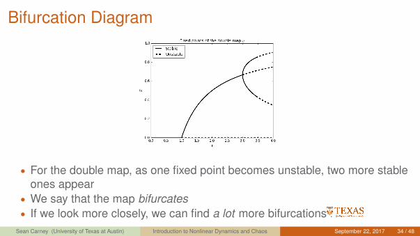
Bifurcation Diagram

• For the double map, as one fixed point becomes unstable, two more stableones appear

• We say that the map bifurcates• If we look more closely, we can find a lot more bifurcations . . .


More Logistic Map ExamplesFor r = 3.84 and r = 3.5 we get periodic behavior again, with period 3 and 4,respectively.


More Logistic Map ExamplesFor r = 3.7, however, we do not get periodic behavior. Instead, we get chaos:

The map never repeats itself in a periodic manner.Sean Carney (University of Texas at Austin) Introduction to Nonlinear Dynamics and Chaos September 22, 2017 36 / 48

Bifurcations

• It turns out chaotic behavior is more common than periodic, orderlybehavior

• With a great bit of help from a computer, we can visualize this nicely . . .


Bifurcation Diagram

• We plot xt versus the parameter r• For each r, we start the map at x0 = 0.1• We let the map run for t = 200 time steps• Then, we start plotting xt versus r for 1400 more time steps• (note: there will be a lot of points plotted for each r)


Bifurcation DiagramWe get a remarkable picture!

What happens if we zoom in one particular section?Sean Carney (University of Texas at Austin) Introduction to Nonlinear Dynamics and Chaos September 22, 2017 39 / 48

Bifurcation DiagramWe get a remarkable picture!

What happens if we zoom in one particular section?Sean Carney (University of Texas at Austin) Introduction to Nonlinear Dynamics and Chaos September 22, 2017 40 / 48

Bifurcation Diagram

The plot exhibits self-similarity.


Chaos – Sensitivity to Initial ConditionsAnother defining characteristic of chaotic behavior is sensitivity to initialconditions. Consider two different plots of the logistic map, again with r = 3.7,with slightly different initial conditions x0 = 0.34 and y0 = 0.35:


More Examples of Chaos• There are many, many more examples of chaotic dynamical systems• One example from everyday life is the phenomenon of fluid turbulence.• The behavior of fluids exhibits some of the same features as the logistic

map:• sensitivity to initial conditions• unstable equilibrium• seemingly random behavior from deterministic rules• beautiful pictures


Fluid TurbulenceFluids behave according to a complicated set of partial differential equations(PDEs) called the Navier-Stokes equations.

∂u∂t

+∇ · (u u) +∇p−(

1Re

)∆u = 0 (9)

∇ · u = 0 (10)

• u is a velocity field–it meaures how fast and in what direction a fluid ismoving at point in time and space

• p measures pressure at a point in time and space• important: the equation is nonlinear (notice the u u term)• Re is a constant, and measures how turbulent a fluid is• Similar to the parameter r in the logistic map, for different values of Re a

fluid can behave quite differentlySean Carney (University of Texas at Austin) Introduction to Nonlinear Dynamics and Chaos September 22, 2017 44 / 48

Transition to Turbulence–Unstable Equilibrium

Recall the video from earlier showing the flow of fluid in a pipe as Re increases.We’ll see orderly, predictable flow (called laminar flow) transition to chaotic,seemingly random turbulent flow.

Fluid transition to turbulence

This is similar to the logistic map behaving predictably for r < 3 and chaoticallyfor r > 3. Unfortunately, for the more complicated Navier-Stokes system, it ismuch more difficult to predict in general the value of Re for which this transitionoccurs.


https://www.youtube.com/watch?v=BBiR6FWmyv4

Fluid Turbulence

Here is a simulation of fluid convection (called Rayleigh-Benardconvection)–warm fluid at the bottom rises and mixes with cold fluid at the topand creates a beautiful, turbulent mess.

Rayleigh-Benard Convection


https://www.youtube.com/watch?v=OM0l2YPVMf8

Turbulence–$1 Million Problem

• Despite its ubiquity, turbulence is an unsolved problem in mathematics• The Clay Institute offers a $1 million dollar prize to anyone who can prove

whether the Navier-Stokes equations possess unique, smooth solutions forall time

• Clay Institute Millennium Problem

∂u∂t

+∇ · (u u) +∇p−(

1Re

)∆u = 0 (11)

∇ · u = 0 (12)

Maybe you can solve the problem and claim the prize.


http://www.claymath.org/millennium-problems/navier-stokes-equation

Thanks for listening!

Questions?


introduction to nonlinear dynamics and chaos · sean carney (university of texas at austin)...

Documents