Introduction toNumerical Integration

Biostatistics 615/815Lecture 17

Last Lecture

Computer generated “random” numbers

Linear congruential generators• Improvements through shuffling, summing

Importance of using validated generators• Beware of problems with the default rand()

function

Today: Numerical Integration

Strategies for numerical integration

Simple strategies with equally spaced abscissas

Gaussian quadrature methods

Monte-Carlo Integration

The ProblemEvaluate:

When no analytical solution is readily available

Many applications in statistics• Analysis of censored data, • Evaluation of cumulative distributions, etc.

dxxfIb

a∫= )(

The Challenge

Evaluate f(x) as few times as possible

Select appropriate set of abscissas

Select appropriate set of weights

The Basic Approach

Notation

Consider a series of abscissas• x0, x1, x2, …, xn, xn+1

Let these be a constant step size h apart• xi = x0 + i h

Further define:• fi = f(xi)

Two Point Trapezoidal Rule

∫ ⎥⎦⎤

⎢⎣⎡ +≈2

121 2

121)(

x

xffhdxxf

Exact for polynomials up to degree 1• For example, f(x) = 2x + 1

Error proportional to h3 and f(2)

Three Point Simpson's Rule

Exact for polynomials up to degree 3 (not 2!)• Due to some symmetries in derivation

Error proportional to h5 and f(4)

∫ ⎥⎦⎤

⎢⎣⎡ ++≈3

1321 3

134

31)(

x

xfffhdxxf

Four Point Rule

Exact for polynomials up to degree 3• No lucky symmetries this time…

Error proportional to h5 and f(4)

Additional formulas exist for higher orders …

∫ ⎥⎦⎤

⎢⎣⎡ +++≈4

14321 8

389

89

83)(

x

xffffhdxxf

Extended Rules

Combine simple rules along consecutive intervals

Two and three point rules allow for adaptive integration• Gradually add points and check accuracy…

Extended Trapezoidal Rule

∫ ⎥⎦⎤

⎢⎣⎡ ++++=nx

x nffffhdxxf1 2

1...21)( 321

Results from application of trapezoidal rule to consecutive intervals …

Simple C Implementation// Integrates function f(x) between a and b// by evaluating it at the edges of the interval // and at n interior pointsdouble integrate2(double a, double b, double (*f)(double x), int n)

{double h = (b – a) / (n + 1), sum;int i;

sum = 0.5 * ((*f)(a) + (*f)(b));

for (int i = 1; i <= n; i++)sum += (*f)(a + i * h);

return sum * h;}

Extended Simpson Rule

∫ ⎥⎦⎤

⎢⎣⎡ ++++=nx

x nfffffhdxxf1 3

1...34

32

34

31)( 4321

Results from application of Simpson's rule to consecutive intervals …• Note alternating 2/3 and 4/3 weights …

Simple C Implementationdouble integrate3(double a, double b, double (*f)(double x), int n)

{double h, sum; int i;

if (n % 2 == 0) n++; // n must be oddh = (b – a) / (n + 1);

sum = (*f)(a) + (*f)(b) + 4.0 * (*f)(a + h);

for (int i = 2; i <= n; i += 2)sum += 2.0 * (*f)(a + i*h) + 4.0 * (*f)(a + (i + 1)*h);

return sum * h / 3.0;}

Problem …

Knowing the required number of points before hand may not be practical…

Is there a simple way to "add more points" ?

Gradually Adding Points

Can you derive formula for updating integral if points are added in this manner?How would you check if a desired accuracy has been reached?

ROUND0123

After 4rounds

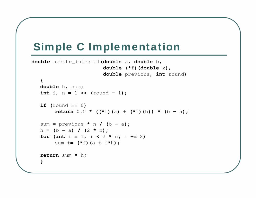
Simple C Implementationdouble update_integral(double a, double b,

double (*f)(double x), double previous, int round)

{double h, sum;int i, n = 1 << (round – 1);

if (round == 0)return 0.5 * ((*f)(a) + (*f)(b)) * (b – a);

sum = previous * n / (b - a);h = (b - a) / (2 * n);for (int i = 1; i < 2 * n; i += 2)

sum += (*f)(a + i*h);

return sum * h;}

Simple C Implementation#define ZEPS 1e-10

double integral(double a, double b, double (*f)(double x),double eps)

{double old = update_integral(a, b, f, 0.0, 0), result; int round = 1;

while (1){result = update_integral(a, b, f, old, round++);if ( fabs(result–old) < eps*(fabs(result)+fabs(old))+ZEPS)

return result;old = result;}

}

Simpson's Extended Rule …

Define TN and T2N to be trapezoidal rule results with N and 2N points, respectively

Then the application of Simpson's rule gives:

NN TTS31

34

2 −=

Simple C Implementationdouble simpson(double a, double b, double (*f)(double x),

double eps){double old = update_integral(a, b, f, 0.0, 0), result; double sold = old, sresult;int round = 1;

while (1){result = update_integral(a, b, f, old, round++);sresult = (4.0 * result – old) / 3.0;if (fabs(sresult–sold)<eps*(fabs(sresult)+fabs(sold))+ZEPS)

return sresult;old = result; sold = sresult;}

}

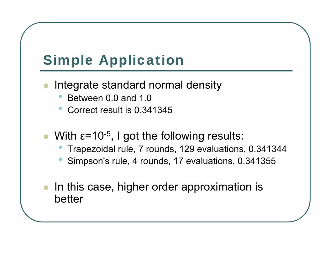
Simple Application

Integrate standard normal density• Between 0.0 and 1.0• Correct result is 0.341345

With ε=10-5, I got the following results:• Trapezoidal rule, 7 rounds, 129 evaluations, 0.341344• Simpson's rule, 4 rounds, 17 evaluations, 0.341355

In this case, higher order approximation is better

Notes on Classical Methods

These methods are most intuitive

Two major applications:• Functions that are not smooth• Function can be pre-calculated along a grid

Exact solutions for polynomials of degree n typically require n or n-1 evaluations

Classical Methods

Function evaluated at equally spaced points

Choice of weights for combining results determines order of approximation

Quadrature Methods

Select locations of function evaluations and weights simultaneously• Abscissas correspond to zeros of particular

classes of orthogonal polynomials

Achieves higher order approximations faster

Gaussian Quadrature

The original idea is due to Gauss (1814)• Described a strategy for choosing appropriate weights and

abscissasWeights and abscissas can be chosen to provide exact results for polynomials of degree 2N – 1 or integrablefunctions of the form W(x) * polynomial(2N – 1)

∫ ∑=

≈b

a

N

jjj xfwdxxf

1)()(

Intuition Behind Idea

Evaluating function at any two points, we can derive exact solution for polynomials of degree 1.• E.g. The trapezoidal rule does this.

But a single well chosen point can achieve the same result…• Which point?

Some Example Abscissas

7

34785485.065214515.065214515.034785485.0

86113631.033998104.033998104.086113631.0

4

55555555.08888889.05555555.0

77459667.00.0

77459667.03

30.10.1

23

1

31

⎟⎟⎟⎟⎟

⎠

⎞

⎜⎜⎜⎜⎜

⎝

⎛

⎟⎟⎟⎟⎟

⎠

⎞

⎜⎜⎜⎜⎜

⎝

⎛

++−−

⎟⎟⎟

⎠

⎞

⎜⎜⎜

⎝

⎛

⎟⎟⎟

⎠

⎞

⎜⎜⎜

⎝

⎛

+

−

⎟⎟⎠

⎞⎜⎜⎝

⎛⎟⎟

⎠

⎞

⎜⎜

⎝

⎛

+

−

MaxDegreeWeightsAbscissasN

C Codedouble gauss3(double a, double b, double (*f)(double x))

{double abscissas[] = {-0.77459667, 0.0, 0.77459667 };double weights[] = {0.55555555, 0.88888889, 0.55555555};double midpoint = 0.5 * (a + b);double h = 0.5 * (b - a);double sum = 0.0;

for (int i = 0; i < 3; i++)sum += weights[i] * (*f)(midpoint + abscissas[i] * h);

return sum * h;}

ComparisonIntegrate standard normal density• Between 0.0 and 1.0• Correct result is 0.341345

With 2, 3 and 4 function evaluations I got:• Using trapezoidal rule

• 0.320457, 0.336261, 0.339096• Using quadrature

• 0.341221, 0.341346, 0.341345• Using Simpson's rule (3 evaluations)

• **********, 0.341529, ***********

Multi-Dimensional Integrals

∫

∫∫ ∫

=

==

=

=

=

=

=

d

c

bx

ax

bx

ax

dy

cy

dyyxfxg

dxxgdxdyyxf

),()(

)(),(

Simplest strategy is to evaluate as a series of one dimensional integrals• Exponential increase in function evaluations

Monte-Carlo Methods

Evaluate and average function at random points

Adaptive methods focus on areas where integrand is most significant• Crucial for multiple dimensions

Monte-Carlo Importance Sampling

Assume N evaluations are available

Evaluate function at kN random points

Divide region of integration into high and low variance regions• Allocate remaining (1 – k)N points so that most

are used in high variance region

Today:

Numerical integration

Classical strategies, with equally spaced abscissas

Discussion of quadrature methods and Monte-Carlo methods

Recommended Reading

Numerical Recipes• Chapters 4.0 – 4.2 for Classical Methods• Chapter 4.5 for Gaussian Quadrature• Chapter 7.8 for Monte-Carlo methods

Available online at:• http://www.nr.com