Introduction to Numerical Methods for SolvingPartial Differential Equations

Benson Muite

benson.muite@ut.eehttp://kodu.ut.ee/˜benson

http://en.wikibooks.org/wiki/Parallel_Spectral_Numerical_Methods

25 March 2015

Outline

• Review• Aim• The heat equation• Methods for solving the heat equation• Fourier Series• The Allen Cahn Equation• Summary• References

Ordinary Differential Equations: Numerical Schemes• Forward Euler method

yn+1 − yn

δt= f

(yn)

• Backward Euler method

yn+1 − yn

δt= f

(yn+1

)• Implicit Midpoint rule

yn+1 − yn

δt= f

(yn+1 + yn

2

)• Crank Nicolson Method

yn+1 − yn

δt=

f(yn+1)+ f (yn)

2• Other Methods: Runge Kutta, Adams Bashforth, Backward

differentiation, splitting

The Heat Equation

• Used to model diffusion of heat, species,• 1D

∂u∂t

=∂2u∂x2

• 2D∂u∂t

=∂2u∂x2 +

∂2u∂y2

• 3D∂u∂t

=∂2u∂x2 +

∂2u∂y2 +

∂2u∂z2

• Not always a good model, since it has infinite speed ofpropagation

• Strong coupling of all points in domain make itcomputationally intensive to solve in parallel

Linear Schrodinger Equation

• Used to model quantum mechanical phenomena and oftenappears in simplified wave propagation models

• 1D

i∂u∂t

=∂2u∂x2

• 2D

i∂u∂t

=∂2u∂x2 +

∂2u∂y2

• 3D

i∂u∂t

=∂2u∂x2 +

∂2u∂y2 +

∂2u∂z2

• Looks like a heat equation with imaginary time• Strong coupling of all points in domain make it

computationally intensive to solve in parallel

The Wave Equation• Used to model propagation of sound, light• 1D

∂2u∂t2 =

∂2u∂x2

• 2D∂2u∂t2 =

∂2u∂x2 +

∂2u∂y2

• 3D∂2u∂t2 =

∂2u∂x2 +

∂2u∂y2 +

∂2u∂z2

• Has finite speed of propagation• Finite signal propagation speed sometimes useful in

parallelization since there is no coupling between gridpoints that are far apart, hence smaller communicationrequirements

• If propagation speed is very fast, communicationrequirements still important

The Poisson Equation

• Used to model static deflection of a drumhead• 1D

f (x) =∂2u∂x2

• 2D

f (x , y) =∂2u∂x2 +

∂2u∂y2

• 3D

f (x , y , z) =∂2u∂x2 +

∂2u∂y2 +

∂2u∂z2

• No time dependence, but also arises in time discretizationsof time dependent partial differential equations

Burgers’ Equation

• Simple model for gas dynamics, also traffic• Inviscid form (can develop shocks)

ut = −uux

• Viscous formut = −uux + εuxx

Navier-Stokes Equations

• Models motion of fluids• Consider incompressible case only (low speed motion

relative to speed of sound)•

ρ

(∂u∂t

+ u · ∇u)

= −∇p + µ∆u

∇ · u = 0.

• p pressure, µ viscosity, ρ, density• 2D u(x , y) = (u(x , y), v(x , y))

• 3D u(x , y , z) = (u(x , y , z), v(x , y , z),w(x , y , z))

Maxwells Equations

• Model propagation of electromagnetic waves•

~Dt −∇× ~H = 0

•~Bt +∇× ~E = 0

• with the relation between the electromagnetic componentsgiven by the constitutive relations:

•~D = εo(x , y , z)~E

•~B = µo(x , y , z)~H

Summary on Models

• Many diverse models• In 2D and 3D, parallel computing is very useful for getting

numerical solutions in reasonable time• Typical applications are in physics, chemistry, biology and

engineering• Related models also appear in social sciences, though

usefulness for predictability of real world data is less clear

Aim to simulate this,

• https://www.flickr.com/photos/kitware/2293740417/in/pool-paraview/

• Visualization around Formula 1 Race Car by Renato N.Elias, Rio de Janeiro, Brazil

or this

• https://www.flickr.com/photos/kitware/2294528826/in/pool-paraview/

• Visualization around Formula 1 Race Car by Renato N.Elias, Rio de Janeiro, Brazil

Maybe even this

• https://youtu.be/FTlJ9l9KTkw• https://youtu.be/MsDgw8_cb90• https://youtu.be/Su8qzC4HHVs

A simple model: The Heat Equation

The Heat Equation

• How does the temperature of the rod vary with time?

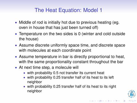
The Heat Equation: Model 1

• Middle of rod is initially hot due to previous heating (eg.oven in house that has just been turned off)

• Temperature on the two sides is 0 (winter and cold outsidethe house)

• Assume discrete uniformly space time, and discrete spacewith molecules at each coordinate point

• Assume temperature in bar is directly proportional to heat,with the same proportionality constant throughout the bar

• At next time step, a molecule will• with probability 0.5 not transfer its current heat• with probability 0.25 transfer half of its heat to its left

neighbor• with probability 0.25 transfer half of its heat to its right

neighbor

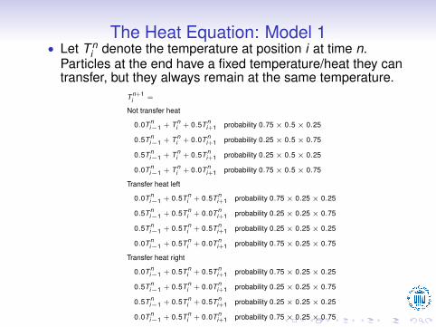
The Heat Equation: Model 1• Let T n

i denote the temperature at position i at time n.Particles at the end have a fixed temperature/heat they cantransfer, but they always remain at the same temperature.

T n+1i =

Not transfer heat

0.0T ni−1 + T n

i + 0.5T ni+1 probability 0.75× 0.5× 0.25

0.5T ni−1 + T n

i + 0.0T ni+1 probability 0.25× 0.5× 0.75

0.5T ni−1 + T n

i + 0.5T ni+1 probability 0.25× 0.5× 0.25

0.0T ni−1 + T n

i + 0.0T ni+1 probability 0.75× 0.5× 0.75

Transfer heat left

0.0T ni−1 + 0.5T n

i + 0.5T ni+1 probability 0.75× 0.25× 0.25

0.5T ni−1 + 0.5T n

i + 0.0T ni+1 probability 0.25× 0.25× 0.75

0.5T ni−1 + 0.5T n

i + 0.5T ni+1 probability 0.25× 0.25× 0.25

0.0T ni−1 + 0.5T n

i + 0.0T ni+1 probability 0.75× 0.25× 0.75

Transfer heat right

0.0T ni−1 + 0.5T n

i + 0.5T ni+1 probability 0.75× 0.25× 0.25

0.5T ni−1 + 0.5T n

i + 0.0T ni+1 probability 0.25× 0.25× 0.75

0.5T ni−1 + 0.5T n

i + 0.5T ni+1 probability 0.25× 0.25× 0.25

0.0T ni−1 + 0.5T n

i + 0.0T ni+1 probability 0.75× 0.25× 0.75

The Heat Equation: Model 1

• DEMO

The Heat Equation: Model 2• Probability is hard!• It takes a long time• May only interested in average temperature/heat, not

instantaneous fluctuations• Take averages

T n+1i = (0.25× 0.5)T n

i−1 + (0.5 + 0.25× 0.5 + 0.25× 0.5)T ni

+ (0.25× 0.5)T ni+1

T n+1i = 0.125T n

i−1 + 0.75T ni + 0.125T n

i+1

or

T n+1i = T n

i +T n

i−1 − 2T ni + T n

i+1

8

• The last line looks like a difference approximation for adifferential equation

The Heat Equation: Model 3

• Let us find a differential equation!• Make the time increment small

T n+1i = T n

i +T n

i−1 − 2T ni + T n

i+1

8T n+1

i − T ni

δt=

T ni−1 − 2T n

i + T ni+1

8δt

The Heat Equation: Model 3

• Let us find a differential equation!• Make the space increment small

T n+1i − T n

iδt

=T n

i−1 − 2T ni + T n

i+1

8δt

T n+1i − T n

iδt

=(δx)2

8δt

T ni−1−T n

iδx − T n

i −T ni+1

δxδx

• Let δx → 0 and δt → 0 such that (δx)2 = δt we get

∂T∂t

=18∂2T∂x2

• Constant in continuum formulation depends on physicsand is usually measured experimentally, or determinedfrom microscopic (many particle) simulations.

The Heat Equation: Numerical Solution Methods

• Probabalistic• Finite Difference• Finite Volume• Finite Element• Spectral

Finite Difference Method

• Approximate derivatives by difference quotients• Simple method to derive and implement• Convergence rates tend not to be great• Difficult to use for complicated geometries• Tends to scale well since communication requirements are

low

Finite Difference Method for Heat Equation

• ut = 8uxx

• Using backward Euler time stepping:

un+1i − un

iδt

= 8un+1

i−1 − 2un+1i + un+1

i+1

(δx)2

• Using forward Euler time stepping (strong stabilityrestrictions):

un+1i − un

iδt

= 8un

i−1 − 2uni + un

i+1

(δx)2

Finite Difference Method for Heat Equation

• Simple method to derive and implement• Hardest part for implicit schemes is solution of resulting

linear system of equations• Explicit schemes typically have stability restrictions or can

always be unstable• Convergence rates tend not to be great – to get an

accurate solution, a large number of grid points are needed• Difficult to use for complicated geometries• Tends to scale well since communication requirements are

low

Finite Volume Method for Heat Equation• ∂u

∂t = ∂2u∂x2 or ∂u

∂x = v and ∂u∂t = ∂v

∂x• Consider a cell averaged integral, then use implicit

midpoint rule ∫ xi+1xi

ux dx =∫ xi+1

xivdx

ui+1 − ui =∫ xi+1

xivdx

un+1i+1 +un

i+1−un+1i −un

i2 =

vn+1i+1 +vn

i+1+vn+1i +vn

i2 δx∫ xi+1

xiutdx =

∫ xi+1xi

vx dx∫ xi+1xi

utdx = vi+1 − vi

un+1i+1 +un+1

i −uni+1−un

i2δt δx =

vn+1i+1 +vn

i+1−vn+1i −vn

i2

• Several ways of approximating the integrals. The oneabove is a little unusual, most finite volume schemes useleft sided or right sided approximations.

Finite Volume Method for Heat Equation

• For implicit schemes, hardest part is solving the system ofequations that results

• Explicit schemes parallelize very well, however a largenumber of grid points are usually needed to get accurateresults

• Automated construction of simple finite volume schemes ispossible, making them popular in packages

• No convergence theory for high order finite volumeschemes

• Tricky to do complicated geometries accurately

Finite Element Method for Heat Equation

• ∂u∂t = ∂2u

∂x2

• Assume u(x , t) ≈ u(x , t) =∑

i φi(x)Ti(t), where φi(x) iszero for x > xi+1 and x < xi−1.

• A simple choice is ψ is the triangle hat function, xi+1 − x forx ∈ [xi , xi+1] and x − xi−1 for x ∈ [xi−1, xi ]

• Now need to find Ti(t), which will be evaluated using finitedifferences.

Finite Element Method for Heat Equation

• Consider multiplying the heat equation by a polynomial, φjthat is only non zero over a few grid points, then integrateby parts, ∫ xi+1

xi−1

∂u∂t φidx =

∫ xi+1xi−1

∂2u∂x2φidx∫ xi+1

xi−1

∂u∂t φidx = −

∫ xi+1xi−1

∂u∂x

∂φi∂x dx

Finite Element Method for Heat Equation• Then use implicit midpoint rule∫ xi+1

xi−1

∂u∂t φidx = −

∫ xi+1xi−1

∂u∂x

∂φi∂x dx∫ xi+1

xi−1

un+1−un

δt φidx = −∫ xi+1

xi−1

12

(∂un

∂x + ∂un+1

∂x

)∂φi∂x dx

12

[un+1

i+1 −uni+1

δt φi |xi+1 +un+1

i−1−uni−1

δt φi |xi−1

]2δx

= −12

[12

(∂un+1

∂x

∣∣∣xi+1

+ ∂un

∂x

∣∣∣xi+1

)∂φi∂x

∣∣∣xi+1

]2δx

− 12

[12

(∂un+1

∂x

∣∣∣xi−1

+ ∂un

∂x

∣∣∣xi−1

)∂φi∂x

∣∣∣xi−1

]2δx

• Since φ are known before hand, can re-write this as matrixvector products, so need to solve a linear system at eachtime step.

Finite Element Method for Heat Equation

• Several other ways of approximating the integrals, canextend to multiple dimensions.

• Weak formulation allows for solution of equations wheresecond derivative is not naturally defined

• Large mathematical community developing convergencetheory for these methods

• Well suited to complicated geometries• Rather difficult to implement compared to other schemes

because of integrals that need to be computed• Used in many codes, but typically codes are hand written

to obtain high efficiency• For implicit time discretizations, solving the linear system

of equations that results can be most time consuming part

Fourier Spectral Method for Heat Equation

Fourier Series: Separation of Variables 1

dydt

= y

dyy

= dt∫dyy

=

∫dt

ln y + a = t + beln y+a = et+b

eln yea = eteb

y =eb

ea et

y(t) = cet

Fourier Series: Separation of Variables 2

•∂u∂t

=∂2u∂x2

• Suppose u = X (x)T (t)•

dTdt (t)T (t)

=d2Xdx2 (x)

X (x)= −C,

• Solving each of these separately and then using linearitywe get a general solution

•∞∑

n=0

αn exp(−Cnt) sin(√

Cnx) + βn exp(−Cnt) cos(√

Cnx)

Fourier Series: Separation of Variables 3

• How do we find a particular solution?• Suppose u(x , t = 0) = f (x)

• Suppose u(0, t) = u(2π, t) and ux (0, t) = ux (2π, t) thenrecall

• ∫ 2π

0sin(nx) sin(mx) =

{π m = n0 m 6= n

,∫ 2π

0cos(nx) cos(mx) =

{π m = n0 m 6= n

,∫ 2π

0cos(nx) sin(mx) = 0.

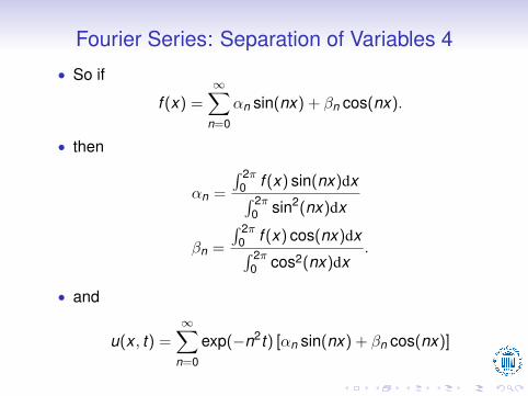
Fourier Series: Separation of Variables 4

• So if

f (x) =∞∑

n=0

αn sin(nx) + βn cos(nx).

• then

αn =

∫ 2π0 f (x) sin(nx)dx∫ 2π

0 sin2(nx)dx

βn =

∫ 2π0 f (x) cos(nx)dx∫ 2π

0 cos2(nx)dx.

• and

u(x , t) =∞∑

n=0

exp(−n2t) [αn sin(nx) + βn cos(nx)]

Fourier Series: Separation of Variables 5

• The Fast Fourier Transform allows one to find goodapproximations to αn and βn when the solution is found ata finite number of evenly spaced grid points

• By rescaling, can consider intervals other than [0,2π)

• Fourier transform also works on infinite intervals, butrequire function to decay to the same constant value at ±∞

Complex Fourier Series

• By using Euler’s formula, one can get a simpler expressionfor a Fourier series where sine and cosine are combined

• u =∑∞

n=−∞ γn exp(inx) x ∈ [0,2π)

Source: http://en.wikipedia.org/wiki/File:Euler%27s_formula.svg

A Computational Algorithm for Computing AnApproximate Fourier Transform 1

• Analytic method of computing Fourier transform can betedious

• Can use quadrature to numerically evaluate Fouriertransforms – O(n2) operations

• Gauss and then Cooley and Tukey found O(n log n)algorithm

• Key observation is to use factorization and recursion• Modern computers use variants of this idea that are more

suitable for computer hardware where moving data is moreexpensive than floating point operations

A Computational Algorithm for Computing AnApproximate Fourier Transform 2

Example pseudo code to compute a radix 2 out of place DFT where x has length that is a power of 2

1: procedure X0,...,N−1(ditfft2(x,N,s))

2: DFT of (x0, xs, x2s, ..., x(N−1)s)

3: if N=1 then4: trivial size-1 DFT of base case5: X0 ← X06: else7: DFT of (x0, x2s, x4s, ...)8: X0,...,N/2−1 ← ditfft2(x,N/2, 2s)

9: DFT of (xs, xs+2s, xs+4s, ...)

10: XN/2,...,N−1 ← ditfft2(x + s,N/2, 2s)

11: Combine DFTs of two halves into full DFT12: for k = 0→ N/2− 1 do13: t ← Xk14: Xk ← t + exp(−2πik/N)Xk+N/2

15: Xk+N/2 ← t − exp(−2πik/N)Xk+N/2

16: end for17: end if18: end procedure

Sources: http://en.wikipedia.org/wiki/Cooley%E2%80%93Tukey_FFT_algorithm,

http://cnx.org/content/m16336/latest/

The Heat Equation: Finding Derivatives andTimestepping

• Letu(x) =

∑k

uk exp(ikx)

• thendνudxν

=∑

(ik)ν uk exp(ikx).

• Consider ut = uxx , which is approximated by

∂uk

∂t= (ik)2uk

un+1k − un

kδt

= (ik)2un+1k

un+1k [1− δt(ik)2] = un

k

un+1k =

unk

[1− δt(ik)2].

The Heat Equation: Finding Derivatives andTimestepping

• Python demonstration

The Allen Cahn Equation: Implicit-Explicit Method

• Consider ut = εuxx + u − u3, which is approximated bybackward Euler for the linear terms and forward Euler forthe nonlinear terms

∂u∂t

= ε(ik)2u + u − u3

un+1 − un

δt= ε(ik)2 ˆun+1 + un − ˆ(un)3

The Allen Cahn Equation: Implicit-Explicit Method

• Python demonstration

Key Concepts

• Differential equations used to model physical phenomena -approximate model

• Microscopic model can suggest ways to find approximatesolutions on computers

• Several methods introduced, probabilistic, finite difference,finite element, spectral (Fourier transform)

• Need to check simulations for discretization errors, thenbefore using for prediction, understand modeling errors

• Time stepping, Forward Euler, Backward Euler, ImplicitMidpoint Rule, Implicit-Explicit

References• Barth, T. and Ohlberger, M. “Finite Volume Methods: Foundation and Analysis”

https://archive.org/details/nasa_techdoc_20030020790

• Boyd, J.P. “Chebyshev and Fourier Spectral Methods” 2nd. edition http://www-personal.umich.edu/˜jpboyd/BOOK_Spectral2000.html

• Chen G., Cloutier B., Li N., Muite B.K., Rigge P. and Balakrishnan S., Souza A.,West J. “Parallel Spectral Numerical Methods” http://shodor.org/petascale/materials/UPModules/Parallel_Spectral_Methods/

• Corral M. Vector Calculus http://www.mecmath.net/• Cooley J.W. and Tukey J.W. “An algorithm for the machine calculation of complex

Fourier series” Math. Comput. 19, 297–301, (1965)• Eymard, R. Gallouet, T. and Herbin, R. “Finite Volume Methods”

http://www.cmi.univ-mrs.fr/˜herbin/BOOK/bookevol.pdf

• Greenbaum A. and Chartier T.P. Numerical Methods Princeton University Press(2012)

• Heideman M.T., Johnson D.H. and Burrus C.S. “Gauss and the History of theFast Fourier Transform” IEEE ASSP Magazine 1, 14–21, (1984)

• Ketcheson, D. “Hyperpython” https://github.com/ketch/HyperPython/• Lawler, G.F. “Random Walk and the Heat Equation” American Mathematical

Society (2010)• Macqueron, C. “Computational Fluid Dynamics Modeling of a wood-burning

stove-heated sauna using NIST’s Fire Dynamics Simulator”http://arxiv.org/abs/1404.6774

References

• McGrattan, K. et al. Fire Dynamics Simulatorhttp://www.nist.gov/el/fire_research/fds_smokeview.cfm

• Petersen W.P. and Arbenz P. Introduction to Parallel Computing Oxford UniversityPress (2004)

• Quarteroni, A. Sacco, R. and Saleri, F. “Numerical Mathematics”http://link.springer.com/book/10.1007%2Fb98885

• Sauer T. Numerical Analysis Pearson (2012)• Suli, E. “Finite element methods for partial differential equations”

people.maths.ox.ac.uk/suli/fem.pdf

• Trefethen, L.N. “Finite Difference and Spectral Methods for Ordinary and PartialDifferential Equations”http://people.maths.ox.ac.uk/trefethen/pdetext.html

• Vainikko E. “Scientific Computing Lectures”https://courses.cs.ut.ee/2013/scicomp/fall/Main/Lectures

• Vainikko E. Fortran 95 Ja MPI Tartu Ulikool Kirjastus (2004)http://kodu.ut.ee/˜eero/PC/F95jaMPI.pdf

Acknowledgements

• Oleg Batrasev

• Leonid Dorogin

• Michael Quell

• Eero Vainikko

• The Blue Waters Undergraduate Petascale Education Programadministered by the Shodor foundation

• The Division of Literature, Sciences and Arts at the University ofMichigan

Extra Slides

Fun with Fourier Series

• A Fourier series can represent a regular k-gon in thecomplex plane

• f (t) =∑+∞

n=−∞(1 + kn)−2 exp [i(1 + kn)t ] t ∈ (−π, π)

Robert, A “Fourier Series of Polygons” Amer. Math. Monthly 101(5) pp. 420-428 (1994)

Schonberg, IJ “The Finite Fourier Series And Elementary Geometry” Amer. Math. Monthly 57(6) pp. 390-404 (1950)

Monte Carlo Method: A Probabilistic Way to CalculateIntegrals

• Recall

f =1

b − a

∫ b

af (x) dx

• Hence given f ∫ b

af (x)dx = (b − a)f

• Doing the same in 2 dimensions and estimating the errorusing the standard deviation∫∫

R

f (x , y) dA ≈ A(R)f ± A(R)

√f 2 − (f )2

N,

• Approximate f by random sampling

f ≈∑N

i=1 f (xi , yi)

Nand f 2 ≈

∑Ni=1(f (xi , yi))2

N

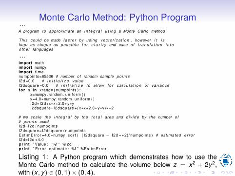
Monte Carlo Method: Python Program” ” ”A program to approximate an i n t e g r a l using a Monte Car lo method

This could be made f a s t e r by using v e c t o r i z a t i o n , however i t i skept as simple as poss ib le f o r c l a r i t y and ease of t r a n s l a t i o n i n t oo ther languages

” ” ”import mathimport numpyimport t imenumpoints=65536 # number o f random sample po in t sI2d =0.0 # i n i t i a l i z e valueI2dsquare =0.0 # i n i t i a l i z e to a l low f o r c a l c u l a t i o n o f var iancefor n in xrange ( numpoints ) :

x=numpy . random . uni form ( )y=4.0∗numpy . random . uni form ( )I2d=I2d+x∗x+2.0∗y∗yI2dsquare=I2dsquare +( x∗x+2.0∗y∗y)∗∗2

# we scale the i n t e g r a l by the t o t a l area and d i v i d e by the number o f# po in t s usedI2d=I2d / numpointsI2dsquare=I2dsquare / numpointsEst imError =4.0∗numpy . s q r t ( ( I2dsquare − I2d ∗∗2)/ numpoints ) # est imated e r r o rI2d=I2d∗4.0pr in t ” Value : %f ” %I2dpr in t ” E r ro r est imate : %f ” %Est imError

Listing 1: A Python program which demonstrates how to use theMonte Carlo method to calculate the volume below z = x2 + 2y2,with (x , y) ∈ (0,1)× (0,4).

Sample Results of Monte Carlo Program

N Value Error Estimate16 37.09 +/- 10.89

256 44.49 +/- 2.404096 44.50 +/- 0.6065536 43.80 +/- 0.14∞ 44 0.0

See http://en.wikibooks.org/wiki/Parallel_Spectral_Numerical_Methods/Introduction_to_Parallel_Programming for more information