introduction to parallel computing - fz-juelich.de
TRANSCRIPT

Mitg
lied
de
r H
elm
ho
ltz-G
em
ein
sch
aft
Introduction to
Parallel Computing
2013 | Bernd Mohr
Institute for Advanced Simulation (IAS)
Jülich Supercomputing Centre (JSC)

2013 JSC 2
Contents
• Introduction
Terminology
Parallelization example (crash simulation)
• Evaluating program performance
• Architectures
Distributed memory
Shared memory
Hybrid systems
• Parallel programming
Message passing, MPI
Multithreading, OpenMP
Accelerators, OpenACC
• Debugging + Parallel program performance analysis
• Future issues for HPC

2013 JSC 3
INTRODUCTION
2013 JSC 4
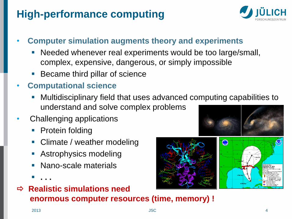
High-performance computing
• Computer simulation augments theory and experiments
Needed whenever real experiments would be too large/small,
complex, expensive, dangerous, or simply impossible
Became third pillar of science
• Computational science
Multidisciplinary field that uses advanced computing capabilities to
understand and solve complex problems
• Challenging applications
Protein folding
Climate / weather modeling
Astrophysics modeling
Nano-scale materials
. . .
Realistic simulations need
enormous computer resources (time, memory) !

2013 JSC 5
Supercomputer
• Supercomputers:
Current most powerful and effective
computing systems
• Supercomputer (in the 1980’s and 1990’s)
Very expensive, custom-built
computer systems
• Supercomputer (since end of 1990’s)
Large number of “off-the-shelf”
components
“Parallel Computing”
2013 JSC 6
Why use Parallel Computers?
• Parallel computers can be the only way to achieve
specific computational goals at a given time
Sequential system is too “slow”
Calculation takes days, weeks, months, years, …
use more than one processor to get calculation faster
Sequential system is too “small”
Data does not fit into the memory
use parallel system to get access to more memory
• [More and more often] You have a parallel system ( multicore)
and you want to make use of its special features
• Your advisor / boss tells you to do it ;-)
2013 JSC 7
Parallel Computing Thesaurus
• Parallel Computing
Solving a task by simultaneous use of multiple processors, all
components of a unified architecture
• Distributed Computing (Grid)
Solving a task by simultaneous use of multiple processors of
isolated, often heterogeneous computers
• Embarrassingly Parallel
Solving many similar, but independent, tasks; e.g., parameter
sweeps. Also called farming
• Supercomputing
Use of the fastest and biggest machines to solve large problems
• High Performance Computing (HPC)
Solving a problem via supercomputers + fast networks + large
storage + visualization

2013 JSC 8
• Application programmer needs to
Distribute data
to memories
Distribute work
to processors
Organize and
synchronize work
and dataflow
• Extra constraint
Do it with least resources
most effective way
Programming Parallel Computers

2013 JSC 9
Example: Crash Simulation
• A greatly simplified model based on parallelizing a crash simulation for
a car company
• Such simulations save a significant amount of money and time
compared to testing real cars
• Example illustrates various phenomena which are common to a great
many simulations and other large-scale applications
2013 JSC 10
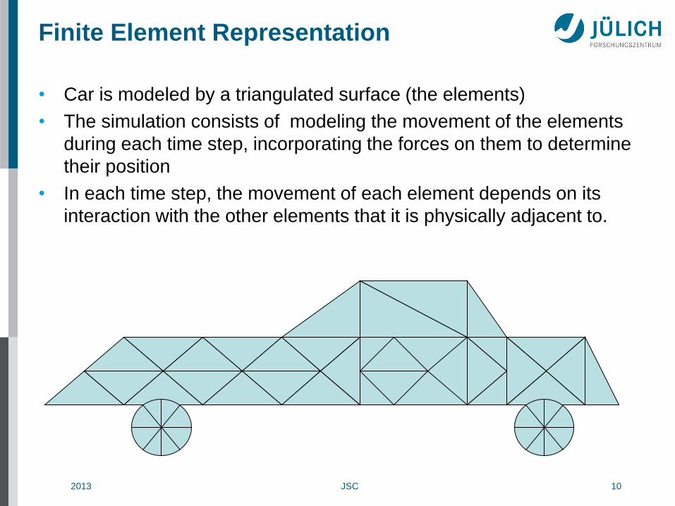
Finite Element Representation
• Car is modeled by a triangulated surface (the elements)
• The simulation consists of modeling the movement of the elements
during each time step, incorporating the forces on them to determine
their position
• In each time step, the movement of each element depends on its
interaction with the other elements that it is physically adjacent to.

2013 JSC 11
Basic Serial Crash Simulation
1. For all elements
2. Read State(element), Properties(element),
NeighborList(element)
3. For time = 1 to end_of_simulation
4. For element = 1 to num_elements
5. Compute State(element) for next time step
based on previous state of element and its neighbors,
and on properties of element
2013 JSC 12
Simple Approach to Parallelization
• Parallel computer cluster based on PC-like processors linked with a
fast network ( distributed memory computer), where processors
communicate via messages ( message passing)
• Cannot parallelize time, so parallelize space
• Distribute elements to processors ( data distribution)
• Each processor updates the positions of the elements stored in its
memory ( owner computes)
• All machines run the same program ( SPMD)

2013 JSC 13
A Distributed Car
2013 JSC 14
Basic Parallel Crash Simulation
• Concurrently for all processors P
1. For all elements assigned to P
2. Read State(element), Properties(element),
NeighborList(element)
3. For time = 1 to end_of_simulation
4. For element = 1 to num_elements-in-P
5. Compute State(element) for next time step
based on previous state of element and its neighbors,
and on properties of element
6. Exchange state information for neighbor elements
located in other processors
2013 JSC 15
Important Issues
• Allocation: How are elements assigned to processors?
Typically, (initial) element assignment determined by serial
preprocessing using domain decomposition approaches
Sometimes dynamic re-allocation ( load-balancing) necessary
• Separation: How does processor keep track of adjacency info for
neighbors in other processors?
Use ghost cells (halo) to copy remote neighbors, add transition
table to keep track of their location and which local elements are
copied elsewhere

2013 JSC 16
Halos
2013 JSC 17
Important Issues II
• Update: How does a processor use State(neighbor) when it does not
contain the neighbor element?
Could request state information from processor containing
neighbor. However, more efficient if that processor sends it
• Coding and Correctness: How does one manage the software
engineering of the parallelization process?
Utilize an incremental parallelization approach, building in
scaffolding
Constantly check test cases to make sure answers correct
• Efficiency: How do we evaluate the success of the parallelization?
Evaluate via speedup or efficiency metrics
2013 JSC 18
EVALUATING
PROGRAM PERFORMANCE
2013 JSC 19
Evaluating Parallel Programs
• An important component of effective parallel computing is determining
whether the program is performing well.
• If it is not running efficiently,
or cannot be scaled to the targeted number of processors,
one needs to determine the causes of the problem
performance analysis
tool support available
and then develop better approaches
tuning or optimization
very little tools support
difficult as often application and platform specific
2013 JSC 20
Definitions
• For a given problem A, let
SerTime(n) = Time of the best serial algorithm to solve A
for input of size n
ParTime(n,p) = Time of the parallel algorithm + architecture
to solve A for input size n, using p processors
Note that SerTime(n) ≤ ParTime(n,1)
• Then
Speedup(p) = SerTime(n) / ParTime(n,p)
Work(p) = p • ParTime(n,p)
Efficiency(p) = SerTime(n) / [p • ParTime(n,p)]

2013 JSC 21
Definitions II
• In general, expect
0 ≤ Speedup(p) ≤ p
Serial work ≤ Parallel work < ∞
0 ≤ Efficiency ≤ 1
• Linear speedup: if there is a constant c > 0 so that speedup is at
least c • p. Many use this term to mean c = 1.
• Perfect or ideal speedup: speedup(p) = p
• Superlinear speedup: speedup(p) > p (efficiency > 1)
Typical reason: Parallel computer has p times more memory
(cache), so higher fraction of program data fits in memory instead
of disk (cache instead of memory)
Parallel version is solving slightly different, easier problem or
provides slightly different answer

2013 JSC 22
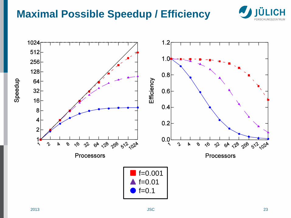
Amdahl’s Law
• Amdahl [1967] noted:
Given a program, let f be the fraction of time spent on operations
that must be performed serially (not parallelizable work). Then for p
processors:
1
Speedup(p) ≤
f + (1 – f)/p
Thus no matter how many processors are used
Speedup(p) ≤ 1/f
Unfortunately, f is typically 5 – 20%
2013 JSC 23
Maximal Possible Speedup / Efficiency
f=0.001
f=0.01
f=0.1

2013 JSC 24
Amdahl’s Law II
• Amdahl was an optimist
Parallelization might require extra work, typically
Communication
Synchronization
Load balancing
Amdahl convinced many people that general-purpose parallel
computing was not viable
• Amdahl was a pessimist
Fortunately, we can break the law!
Find better (parallel) algorithms with much smaller values of f
Superlinear speedup because more data fits cache/memory
Scaling: exploit large parallel machines by scaling the problem
size with the number of processes

2013 JSC 25
Scaling
• Amdahl scaling
• But why not … ?
2013 JSC 26
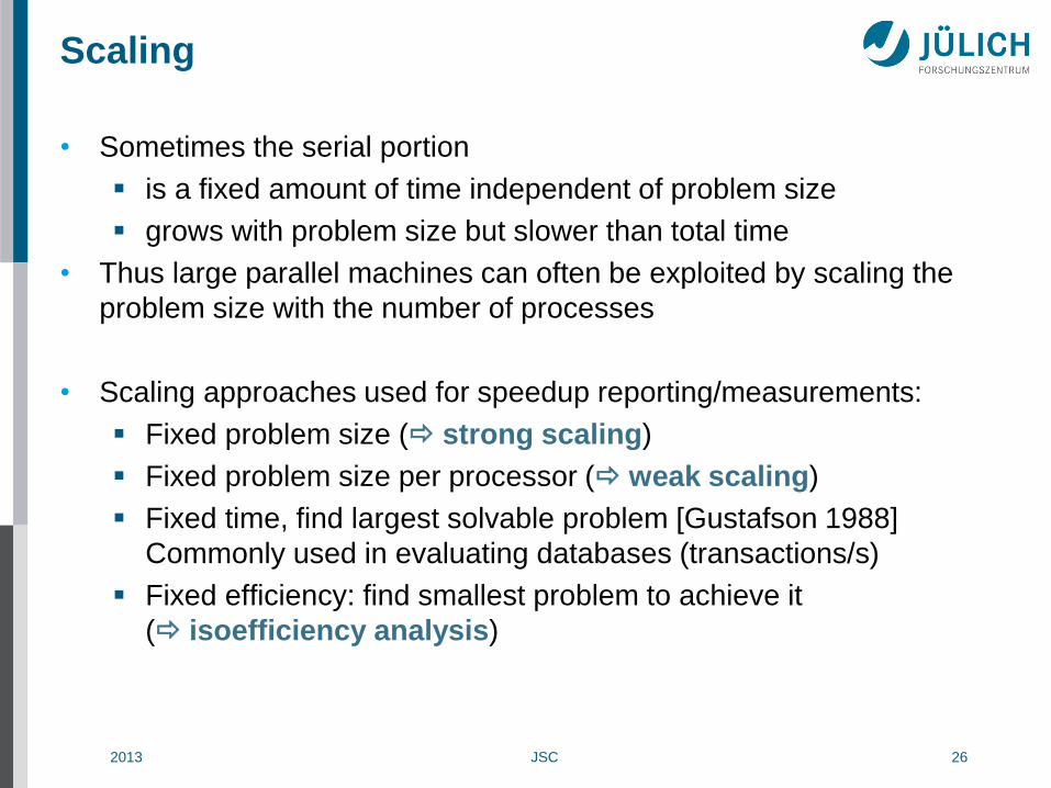
Scaling
• Sometimes the serial portion
is a fixed amount of time independent of problem size
grows with problem size but slower than total time
• Thus large parallel machines can often be exploited by scaling the
problem size with the number of processes
• Scaling approaches used for speedup reporting/measurements:
Fixed problem size ( strong scaling)
Fixed problem size per processor ( weak scaling)
Fixed time, find largest solvable problem [Gustafson 1988]
Commonly used in evaluating databases (transactions/s)
Fixed efficiency: find smallest problem to achieve it
( isoefficiency analysis)
2013 JSC 27
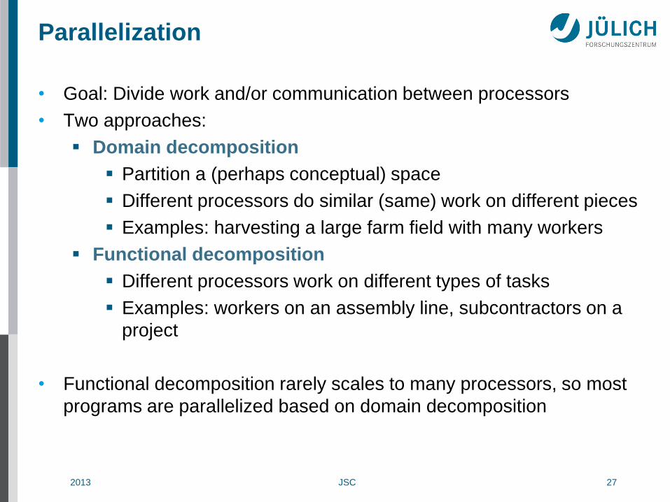
Parallelization
• Goal: Divide work and/or communication between processors
• Two approaches:
Domain decomposition
Partition a (perhaps conceptual) space
Different processors do similar (same) work on different pieces
Examples: harvesting a large farm field with many workers
Functional decomposition
Different processors work on different types of tasks
Examples: workers on an assembly line, subcontractors on a
project
• Functional decomposition rarely scales to many processors, so most
programs are parallelized based on domain decomposition

2013 JSC 28
• Goal
Divide work between
processors equally
work load on all
processors
is the same
load balancing
• Difficulties
Unknown distribution
of work
Dynamic changes in
work load
Parallelization: Load Balancing
2013 JSC 29
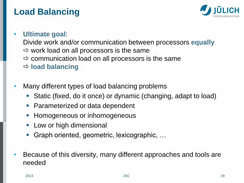
Load Balancing
• Ultimate goal:
Divide work and/or communication between processors equally
work load on all processors is the same
communication load on all processors is the same
load balancing
• Many different types of load balancing problems
Static (fixed, do it once) or dynamic (changing, adapt to load)
Parameterized or data dependent
Homogeneous or inhomogeneous
Low or high dimensional
Graph oriented, geometric, lexicographic, …
• Because of this diversity, many different approaches and tools are
needed

2013 JSC 30
Load Balancing: Complicating Factors
• Objects being computed do not have a simple dependency pattern
among themselves, so communication load-balancing is difficult to
achieve
• Objects do not have uniform computational requirements, and it may
not initially be clear which ones need more time
• If objects are repeatedly updated (such as elements in the crash
simulation), the computational load of an object may vary over
iterations
• Objects may be created dynamically and in an unpredictable manner,
complicating both computational and communicational load balance

2013 JSC 31
ARCHITECTURE

2013 JSC 32
Architectural Taxonomies
• The classifications of parallel computers are in terms of hardware; but
there are natural software analogues
• These classifications provide ways to think about problems and their
solution.
• Note: many real systems blend approaches, and do not exactly
correspond to the classifications
2013 JSC 33
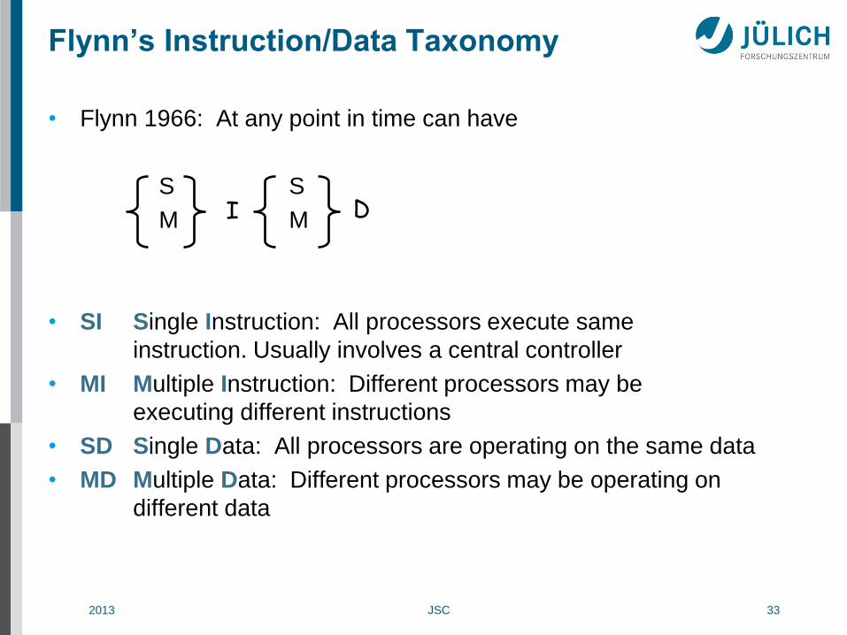
Flynn’s Instruction/Data Taxonomy
• Flynn 1966: At any point in time can have
S S
M M
• SI Single Instruction: All processors execute same
instruction. Usually involves a central controller
• MI Multiple Instruction: Different processors may be
executing different instructions
• SD Single Data: All processors are operating on the same data
• MD Multiple Data: Different processors may be operating on
different data
I D
2013 JSC 34
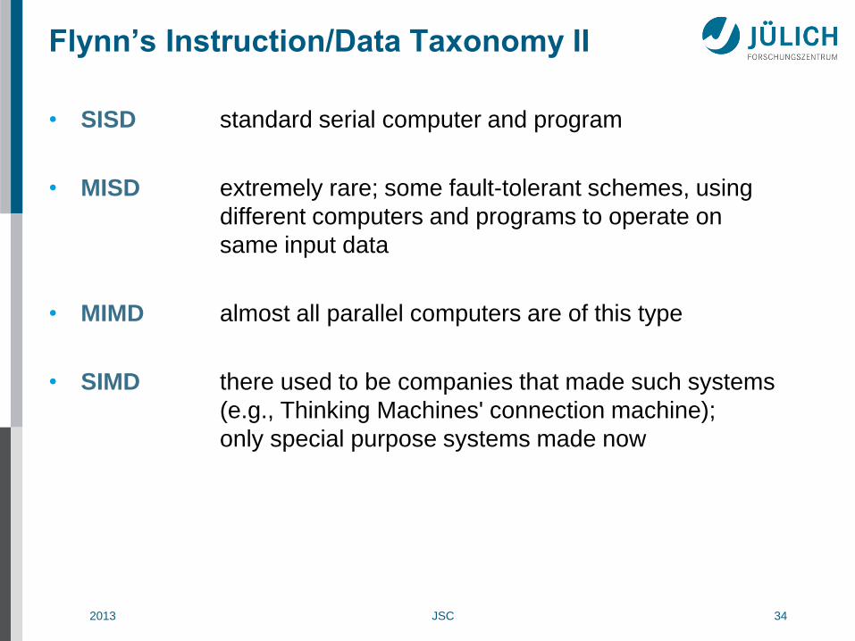
Flynn’s Instruction/Data Taxonomy II
• SISD standard serial computer and program
• MISD extremely rare; some fault-tolerant schemes, using
different computers and programs to operate on
same input data
• MIMD almost all parallel computers are of this type
• SIMD there used to be companies that made such systems
(e.g., Thinking Machines' connection machine);
only special purpose systems made now
2013 JSC 35
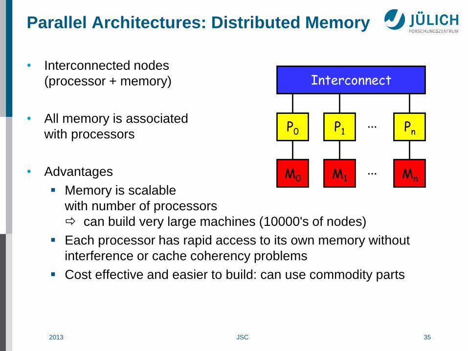
Parallel Architectures: Distributed Memory
• Interconnected nodes
(processor + memory)
• All memory is associated
with processors
• Advantages
Memory is scalable
with number of processors
can build very large machines (10000's of nodes)
Each processor has rapid access to its own memory without
interference or cache coherency problems
Cost effective and easier to build: can use commodity parts
Interconnect
M0 M1 Mn ...
P0 P1 Pn ...
2013 JSC 36
Parallel Architectures: Distributed Memory II
• Disadvantages
To retrieve information from another processor’s memory a
message must be sent over the network to the home processor
Programmer is responsible for many of the details of the
communication; easy to make mistakes
Explicit data distribution
Explicit communication via messages
Explicit synchronization
May be difficult to distribute the data structures, often additional
data structures needed (ghost cells, location tables, …)
• Programming Models
Message passing: MPI, PVM, shmem, LAPI, ELAN, ...
Data parallelism: HPF

2013 JSC 37
• Further classification based on how memory is accessed
NORMA (NO Remote Memory Access)
Nodes connected via network adaptors
to external networks (switches)
NOW (Network of Workstations)
COW (Cluster of Workstations)
RMA (Remote Memory Access)
Processors connected via internal
special interconnect hardware
Often allows one-sided memory
transfers (get, put)
MPP (Massively Parallel Processing)
system
Parallel Architectures: Distributed Memory III
Network or Switch
M0 M1 Mn ...
P0 P1 Pn ...
Internal Networks
M0 M1 Mn ...
P0 P1 Pn ...
Example: Cray T3E
Example: PC Cluster

2013 JSC 38
Parallel Architectures: Shared Memory
• More exact: shared address space
accessible by all processors
physical memory modules may be
distributed
• Processors may have local memory
(e.g., caches) to hold copies of
some global memory. Consistency of
these copies is usually maintained by special hardware
• Programming Models
Automatic parallelization via compiler
Explicit threading (e.g. POSIX threads)
OpenMP
[MPI]
Interconnect
P0 P1 Pn
Memory
...
M0 M1 Mn ... Memory
2013 JSC 39
Parallel Architectures: Shared Memory II
• Advantages
Global address space is user-friendly; program may be able to use
global data structures efficiently and with little modification
Typically easier to program
Implicit communication via (shared) data
But still explicit synchronization!
Data sharing (communication) between tasks is very fast
• Disadvantages
Requires special expensive hardware for efficient (scalable)
memory access and cache coherence
Therefore not very scalable (10 to 100's of nodes)

2013 JSC 40
Parallel Architectures: Shared Memory III
• Further classification based on memory access time:
UMA (Uniform Memory Access)
Equal access times to memory from each processor
Almost always cache-coherent
Interconnects:
Bus Crossbar
Least scalable architecture
Also used: SMP (Symmetrical Multi Processor)
Example: Current Multi-core processors
P0 P1 P3
M0 M1 M3 M2
P2 P0 P1 P3
M0 M1 M3 M2
P2
2013 JSC 41
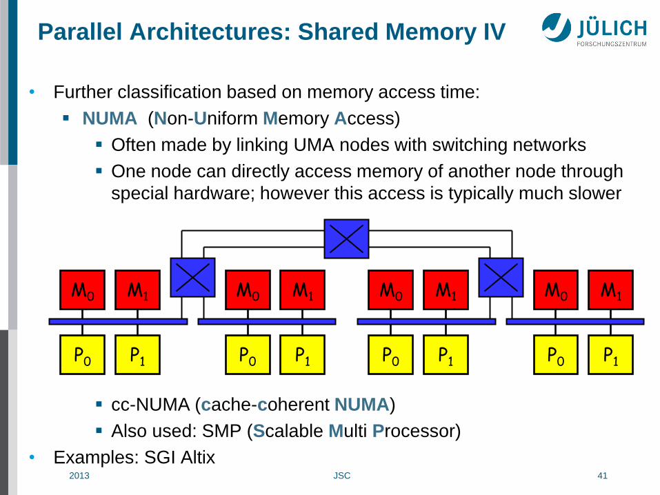
Parallel Architectures: Shared Memory IV
• Further classification based on memory access time:
NUMA (Non-Uniform Memory Access)
Often made by linking UMA nodes with switching networks
One node can directly access memory of another node through
special hardware; however this access is typically much slower
cc-NUMA (cache-coherent NUMA)
Also used: SMP (Scalable Multi Processor)
• Examples: SGI Altix
P0 P1
M0 M1
P0 P1
M0 M1
P0 P1
M0 M1
P0 P1
M0 M1
2013 JSC 42
Shared Memory on Distributed Memory
• It is usually easier to parallelize a program
on a shared memory system
• However, most systems have distributed memory
because of the cost and scalability advantages
• To gain both advantages people investigate using software to emulate
shared memory access
Virtual shared memory: virtualization inside operating system on
the memory page level rarely efficient
Special programming languages or libraries providing a global
address space abstraction
Global arrays
Unified Parallel C (UPC)
Co-Array Fortran (CAF)

2013 JSC 43
• Logical extension of distributed and shared memory architectures
Increased complexity in hardware, software, and programming!!!
• Programming Models
Message passing
Message passing between nodes + multi-threading within nodes
• Examples: IBM BlueGene/P or Cray XT4
Node0 Node1 Noden
Parallel Architectures: Hybrid Systems
Network or Switch
... Interconnect
P0 P1 Pn ...
Memory
Interconnect
P0 P1 Pn ...
Memory
Interconnect
P0 P1 Pn ...
Memory

2013 JSC 44
Parallel Architectures: Hybrid Systems II
• Two typical forms:
• Clusters of shared memory nodes
Number of nodes >> number of processors inside node
Often small, cheaper SMP nodes (rack-mounted, blades)
Sometimes called clumps
Often commodity network (e.g., Gigabit Ethernet)
• Constellation systems
Number of processors inside node > number of nodes
Larger, more expensive UMA or cc-NUMA nodes
Typically special high performance interconnect networks
2013 JSC 45
Accelerators
• Special hardware for accelerating computations
has long tradition in HPC
Floating-point units
SIMD/vector units
MMX, SSE (Intel), 3DNow! (AMD), AltiVec (IBM)
BlueGene double hummer, …
FPGA (Field Programmable Gate Arrays)
Cell-Chip
Main PowerPC core + 8 SPE (Synergistic Processing Elements)
LLNL RoadRunner (Opteron / Cell heterogeneous system)
• Latest trends in HPC:
General Purpose computing on Graphics Processing Units (GPGPU)
Many-core, e.g. Intel MIC

2013 JSC 46
Abstracted x64 + Accelerator Architecture

2013 JSC 47
GPGPU
• Modern GPUs
Have a parallel many-core architecture
Each core capable of running 1000s of threads simultaneously
MIMD blocks with SIMD fine-grain parallelism
Highly parallel structure makes them more effective than general-
purpose CPUs for some (vectorizable) algorithms
• Large HPC clusters with GPU acceleration already built (#GPUs):
Titan (18,688), Tianhe-1A (7168), Nebulae (4640),
Tokyo Tech (4224), …
• Difficult to use hardware effectively
High-level (portable) programming interfaces just evolving
Main disadvantage: data must be moved
to and from main memory to GPU memory
Data locality important, otherwise performance degrades
significantly

2013 JSC 48
Intel Many Integrated Core Architecture (MIC)
• Intel Xeon Phi (2013)
1.1 GHz, up to 61 cores, each 4-way SMT, 512-bit SIMD instructions
• Current systems
Tianhe-2A (48,000), Discover (NASA, 480), MVS-10P (RSC, 416)
Core
L2
TD Core
L2
TD
Core
L2
TD Core
L2
TD
Core
L2
TD Core
L2
TD
Core
L2
TD Core
L2
TD
…
…
…
…
GDDR MC
GDDR MC
GDDR MC
GDDR MC
PCIe
Client
Logic

2013 JSC 49
Parallel Architectures: State of the Art
Network or Switch
...
N0 N1 Nk
Inter- connect
P0 Pn ...
Memory
A0
Am
... Inter- connect
P0 Pn ...
Memory
A0
Am
... Inter- connect
P0 Pn ...
Memory
A0
Am
...
Pi Core0 Core1 Corer
L10 L11 L1
L20 L2r/2
L30
...
... Aj
Router Router
Router
Router Router
Router
Router
Router Router Router
Router Router Router
Router Router Router
Router Router Router
Router Router Router
Router Router Router
Router Router Router
Router Router Router
Router Router Router
or

2013 JSC 50
Example: BSC IBM MareNostrum (2006)

2013 JSC 51
Example: BSC IBM MareNostrum (2006)
• 64-bit IBM PowerPC 970MP
2.3 GHz, 2-way SMP
• 94.21 Teraflop/s peak
63.83 Teraflop/s Linpack
Nov06: #5
Jun12: #465
• 20 TByte memory
• 2,560 JS21 blades
10,240 cores
• Interconnects
Myrinet
Gigabit Ethernet

2013 JSC 52
Example: NUDT Tianhe-2A (2013)
• Node:
2 x 64-bit Intel IvyBridge
+
3 x Intel Xeon Phi
• 54.90 Petaflop/s peak
33.86 Petaflop/s Linpack
Jun13: #1
• 1.4 PByte memory
• 162 racks
• 16,000 nodes
• 3,120,000 cores
• Express-2 Interconnect
(Chinese)
• 17.8 MW

2013 JSC 53
Example: NUDT Tianhe-2A (2013)
• 16,000 Nodes each
2 x 64-bit Intel IvyBridge
2.2 GHz
12-way SMP
3 x Intel Xeon Phi
1.1 GHz,
57 cores
Pictures of
node boards
courtesy of
Taisuke Boku

2013 JSC 54
Example: LLNL Sequoia computer (2012)
• 64-bit IBM PowerPC A2
1.6 GHz, 16-way SMP
• 20.13 Petaflop/s peak
17.17 Petaflop/s Linpack
Jun12: #1
Jun13: #3
• 1.6 PByte memory
• 96 racks
• 98,304 nodes
• 1,572,864 cores
• 5D interconnect
• Water cooling

2013 JSC 55
Example: RIKEN AICS K computer (2011)
• 64-bit Sparc VIIIfx
2.0 GHz, 8-way SMP
• 11.28 Petaflop/s peak
10.51 Petaflop/s Linpack
Nov11: #1
Jun13: #4
• 1.41 PByte memory
• 864 racks
• 88,128 nodes
• 705,024 cores
• 6D interconnect (Tofu)
• Water cooling
2013 JSC 56
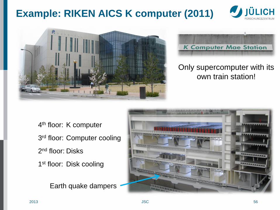
Example: RIKEN AICS K computer (2011)
Only supercomputer with its
own train station!
4th floor: K computer
3rd floor: Computer cooling
2nd floor: Disks
1st floor: Disk cooling
Earth quake dampers

2013 JSC 57
Example: RIKEN AICS K computer (2011)
Building
Earth quake
Security
“wiggle” moves damper
horizontal moves
damper
flexible pipes
Ve
rtic
al m
ove
s
dam
per
2013 JSC 58
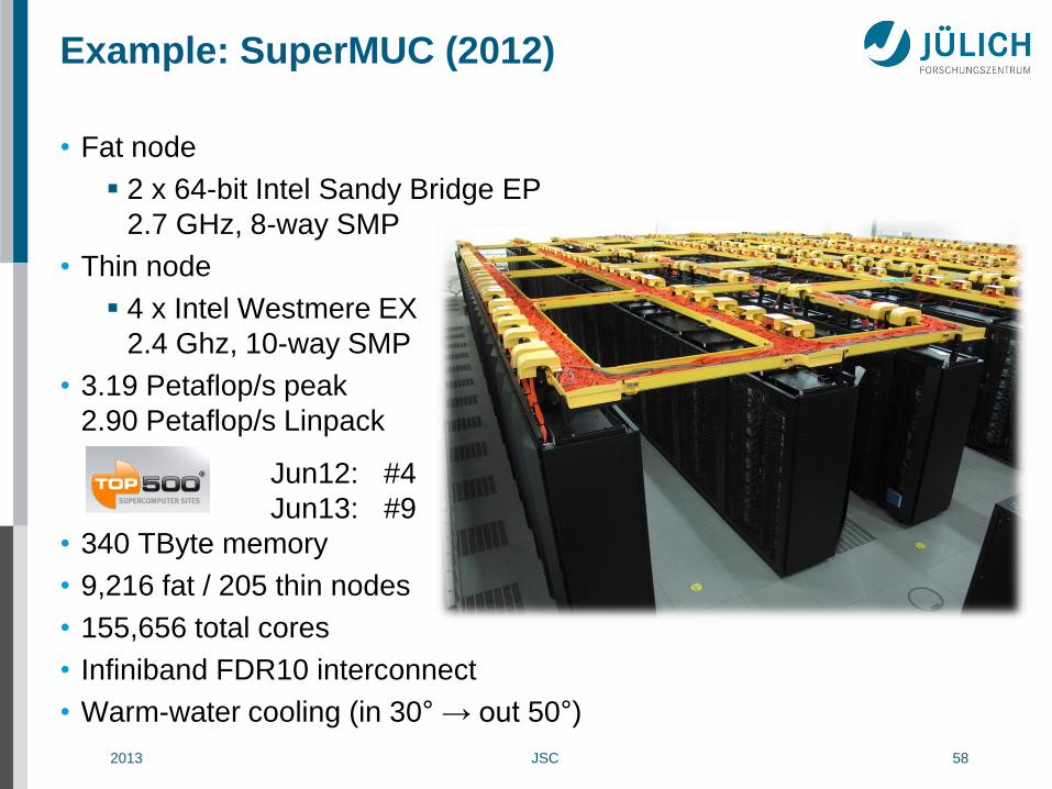
Example: SuperMUC (2012)
• Fat node
2 x 64-bit Intel Sandy Bridge EP
2.7 GHz, 8-way SMP
• Thin node
4 x Intel Westmere EX
2.4 Ghz, 10-way SMP
• 3.19 Petaflop/s peak
2.90 Petaflop/s Linpack
Jun12: #4
Jun13: #9
• 340 TByte memory
• 9,216 fat / 205 thin nodes
• 155,656 total cores
• Infiniband FDR10 interconnect
• Warm-water cooling (in 30° → out 50°)
2013 JSC 59
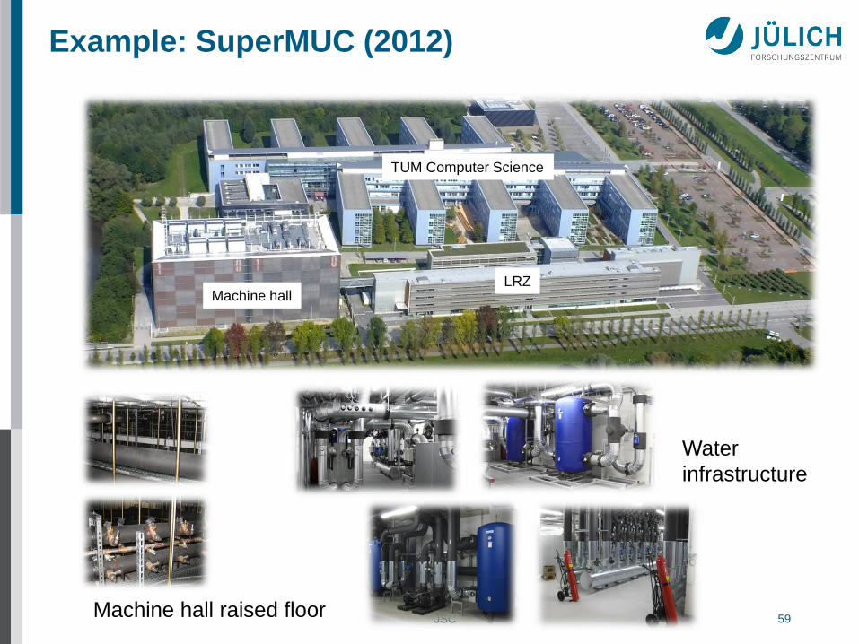
Example: SuperMUC (2012)
TUM Computer Science
LRZ Machine hall
Water
infrastructure
Machine hall raised floor

2013 JSC 60
Example: NSCC Tianhe-1A (2010)
• 64-bit Intel Xeon X5670 6C
2.93 GHz, 6-way SMP
• 4.70 Petaflop/s peak
2.57 Petaflop/s Linpack
Nov10: #1
Jun13: #10
• 262 TByte memory
• 112 racks
• 14,336 Xeon
• 86,016 cores
• 7,168 Nvidia
Tesla M2050
• 2,048 NUDT FT1000 processors
• Galaxy interconnect (Chinese)

2013 JSC 61
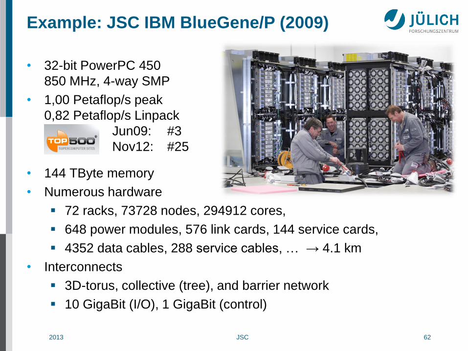
Example: JSC IBM BlueGene/P (2009)
2013 JSC 62
• 32-bit PowerPC 450
850 MHz, 4-way SMP
• 1,00 Petaflop/s peak
0,82 Petaflop/s Linpack
Jun09: #3
Nov12: #25
• 144 TByte memory
• Numerous hardware
72 racks, 73728 nodes, 294912 cores,
648 power modules, 576 link cards, 144 service cards,
4352 data cables, 288 service cables, … → 4.1 km
• Interconnects
3D-torus, collective (tree), and barrier network
10 GigaBit (I/O), 1 GigaBit (control)
Example: JSC IBM BlueGene/P (2009)

2013 JSC 63
• 64-bit PowerPC A1
1.6 GHz, 16-way SMP
each 4-way SMT
• 5.87 Petaflop/s peak
5.00 Petaflop/s Linpack
Nov12: #5
Jun 13: #7
• 448 TByte memory
• 28 racks
• 458,752 cores
• 5D-torus interconnect
• 90% water cooled, 10% air
• 6 racks BG/Q more powerful than 72 racks BG/P!
Example: JSC IBM BlueGene/Q (2012)

2013 JSC 64
2013 JSC 65
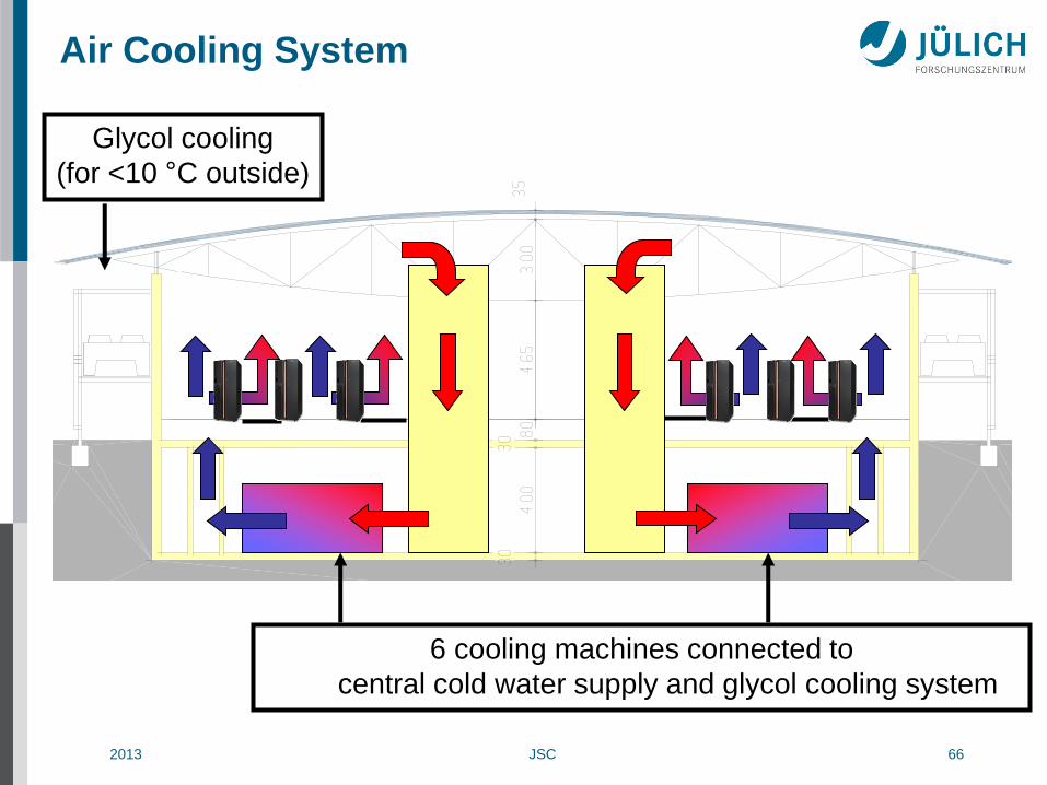
JSC Machine Hall Specifications
• Area: 1000 m²
self supporting roof
• Volume: 6500 m³
• Power supply: 5300 kW
• Floor temperature: 16 °C
• Humidity: 40 – 60 %
• Air exchange rate: 38/h
• Air exchange: 250000 m³/h
• UPS: only for communication and disks
2013 JSC 66
Air Cooling System
Glycol cooling
(for <10 °C outside)
6 cooling machines connected to
central cold water supply and glycol cooling system
2013 JSC 67
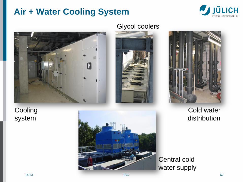
Air + Water Cooling System
Glycol coolers
Cooling
system
Cold water
distribution
Central cold
water supply

2013 JSC 68
Water-Cooled Blue Gene/P
16 C
31 C 35 C
35 C
18 C 24 C
20 C
…
16 C
8 racks
in one
row
9 rows with
8 racks each

2013 JSC 69
JSC: Supply of Cooling Water
Bringing water into
basement
Establishing a room
with pumps to prepare
different inlet temperatures

2013 JSC 70
JSC: Extending the Power Supply
from
1,6 MW
to
5,3 MW

2013 JSC 71
Number of fuses: • 72x3 125 A • 220x1 32 A • 598x1 16 A • 174x1 32 A • 12x3 32 A 1244 total
30 m power distribution panels
nearly 50 km
length of cables
JSC: Power Distribution

2013 JSC 72
Length of the communication cables:
• BG/P: 23 km (copper)
21 km (fiber)
• JUROPA: 20 km (mixed)
• HPC-FF: 16 km (mixed)
80 km
JSC: Supercomputer Networks

2013 JSC 73
JSC: Fire Prevention
Argon bottles
Pressure equalization

2013 JSC 74
Costs (JSC, 2011)
• Jugene (IBM BlueGene/P)
1 Node hour (Quadcore) 0.039 €
Typical job (1 day x 2048 nodes) 1916.92 €
Maximum (1 day x 73728) 69009.41 €
• Juropa (Bull/Sun Intel Nehalem/Infiniband cluster)
1 Node hour (Dual quadcore) 0.39 €
Typical job (12h x 128 nodes) 599.04 €
Maximum (1 day x 3288) 30775.68 €

2013 JSC 76
PARALLEL PROGRAMMING
2013 JSC 77
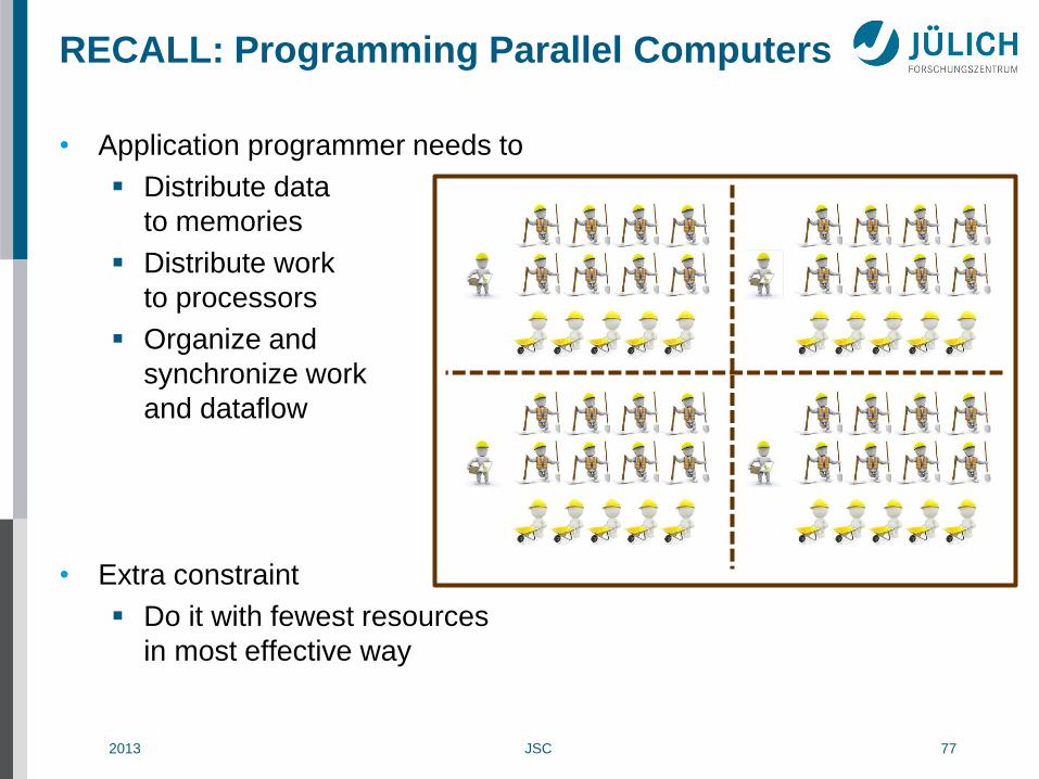
• Application programmer needs to
Distribute data
to memories
Distribute work
to processors
Organize and
synchronize work
and dataflow
• Extra constraint
Do it with fewest resources
in most effective way
RECALL: Programming Parallel Computers

2013 JSC 78
Parallelization Strategies
• Two major computation resources:
Processor
Memory
• Parallelization means
Distributing work among processors
Synchronization of the distributed work
• If memory is distributed it also means
Distributing data
Communicating data between local and remote processors
• Programming models offer combined methods for
Distribution of work & data
Communication and synchronization

2013 JSC 79
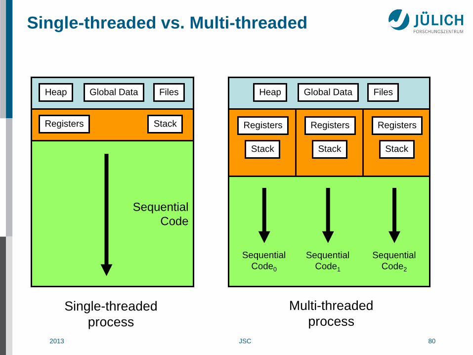
Processes and Threads
• Processes are entities provided by the operating system (OS) to
execute programs
• A typical (sequential) process consists of a thread of execution
executing the program starting with main. The thread can access
A stack for storing local data
A heap for storing dynamic data (e.g., via allocate/malloc/new)
Space for storing global static data
• If OS supports multi-threading, a process can have multiple threads
Can be dynamically created and destroyed at run-time
Each thread can access the heap and global data
Each thread has its own stack!
• Parallel programs
Can use multiple processes + mechanism to communicate
On shared memory computer, use multi-threading
Or combination of both
2013 JSC 80
Single-threaded vs. Multi-threaded
Sequential
Code
Heap Files Global Data
Registers Stack Registers
Stack
Registers
Stack
Registers
Stack
Heap Files Global Data
Single-threaded
process
Multi-threaded
process
Sequential
Code0
Sequential
Code1
Sequential
Code2

2013 JSC 81
Basic Parallel Programming
Paradigm: SPMD
• SPMD: Single Program Multiple Data
• Basic paradigm for implementing parallel programs
• Programmer writes one program
Which is executed on all processors
But written in a way that it works on different parts of the data
• Special cases (e.g., different control flow) is handled
inside the program
if (process_or_thread_id == 42) then
call do_something()
else
call do_something_else()
endif

2013 JSC 82
Programming Models: Message Passing
• Typically used on distributed memory computer systems
• Local (“distributed”) style
SPMD-style program runs locally using local data
• Explicit data distribution, communication and synchronization
High programming overhead
Message passing libraries: MPI, PVM, ...
P0 P1 P2 P3
2013 JSC 83
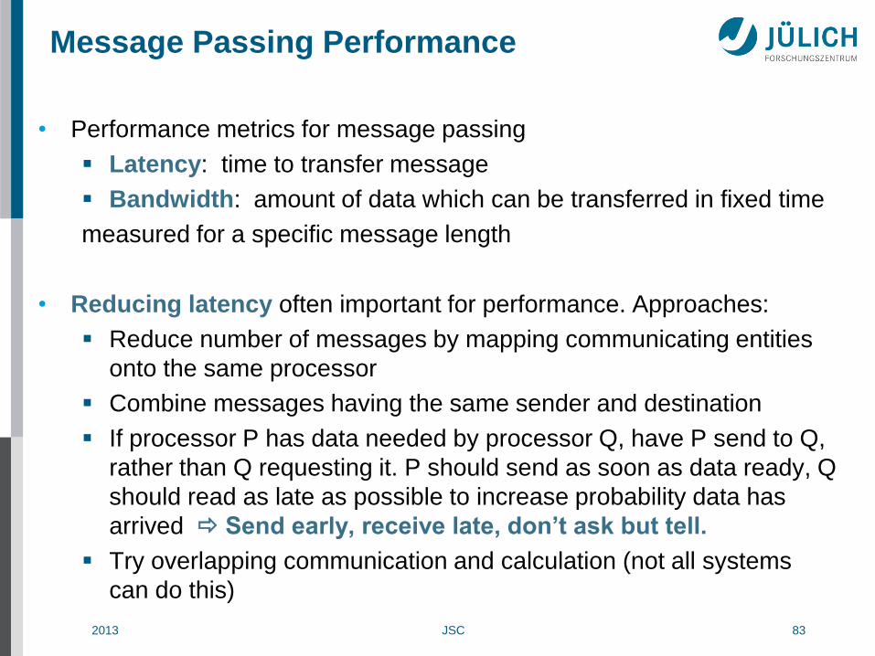
Message Passing Performance
• Performance metrics for message passing
Latency: time to transfer message
Bandwidth: amount of data which can be transferred in fixed time
measured for a specific message length
• Reducing latency often important for performance. Approaches:
Reduce number of messages by mapping communicating entities
onto the same processor
Combine messages having the same sender and destination
If processor P has data needed by processor Q, have P send to Q,
rather than Q requesting it. P should send as soon as data ready, Q
should read as late as possible to increase probability data has
arrived Send early, receive late, don’t ask but tell.
Try overlapping communication and calculation (not all systems
can do this)

2013 JSC 84
Programming Models: MPI
• MPI: Message Passing Interface
• De-facto standard message passing interface
MPI 1.0 in 1994
MPI 1.2 in 1997
MPI 2.0 in 1997
MPI 2.1 in 2008
MPI 2.2 in 2009
MPI 3.0 in 2012
• Library interface
• Language bindings for Fortran, C, C++, [Java]
• Typically used in conjunction with SPMD programming style
• http://www.mpi-forum.org
2013 JSC 85
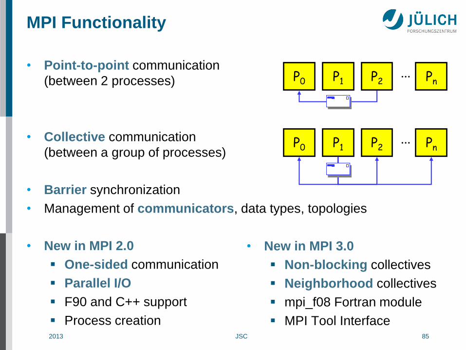
MPI Functionality
• Point-to-point communication
(between 2 processes)
• Collective communication
(between a group of processes)
• Barrier synchronization
• Management of communicators, data types, topologies
• New in MPI 2.0
One-sided communication
Parallel I/O
F90 and C++ support
Process creation
P1 P2 Pn ... P0
P1 P2 Pn ... P0
• New in MPI 3.0
Non-blocking collectives
Neighborhood collectives
mpi_f08 Fortran module
MPI Tool Interface

2013 JSC 86
MPI Functionality
2013 JSC 87
MPI Communicators
• Communicator consists of a process group
and a communication context
• Predefined communicator (representing all processes)
is MPI_COMM_WORLD
• Each message is sent relative to a communicator
• All processes in the process group of the communicator have to take
part in a collective operation
• Operations are provided to:
Determine the number of processes in a communicator
Determine the rank of the executing process relative to a
communicator 0 to N-1
Build new process groups and communicators
2013 JSC 88
MPI Basic Routines
MPI_Init()
Initialize MPI library
Needs to be called once, before all other MPI functions
MPI_Finalize()
Wrap-up / terminates MPI usage
Needs to be called once, after all other MPI functions
MPI_Comm_size(comm, size)
Get total number of processes in communicator comm
MPI_Comm_rank(comm, rank)
Get process identification (rank) within comm

2013 JSC 89
Example: Hello World (MPI), Fortran
program main include 'mpif.h' integer :: ierr, myrank, numprocs call MPI_Init(ierr) call MPI_Comm_rank(MPI_COMM_WORLD, myrank, ierr) call MPI_Comm_size(MPI_COMM_WORLD, numprocs, ierr) write(*,*) "hello from", myrank, "of", numprocs call MPI_Finalize(ierr) end program
Fortran MPI routines:
error code returned in
extra parameter!
2013 JSC 90
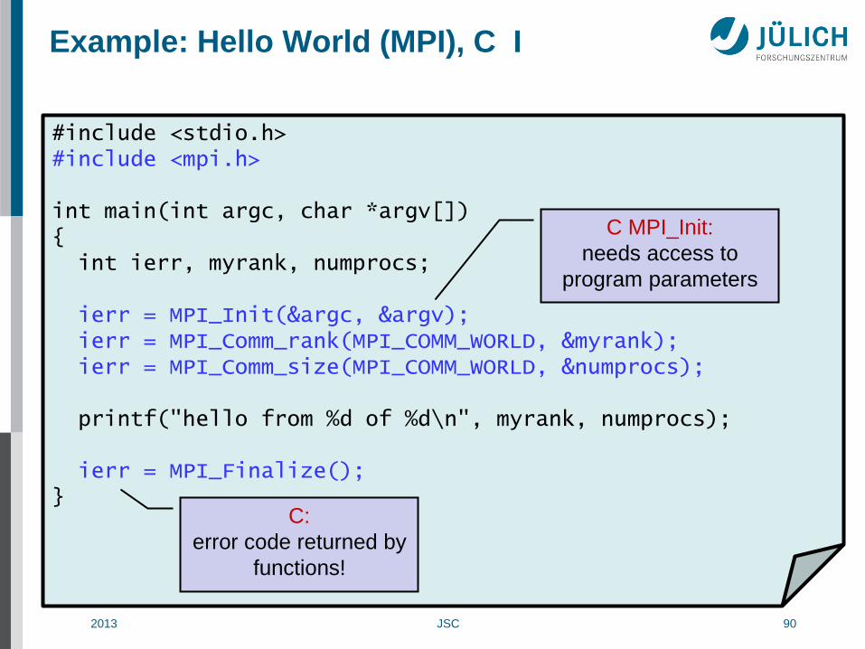
Example: Hello World (MPI), C I
#include <stdio.h> #include <mpi.h> int main(int argc, char *argv[]) { int ierr, myrank, numprocs; ierr = MPI_Init(&argc, &argv); ierr = MPI_Comm_rank(MPI_COMM_WORLD, &myrank); ierr = MPI_Comm_size(MPI_COMM_WORLD, &numprocs); printf("hello from %d of %d\n", myrank, numprocs); ierr = MPI_Finalize(); }
C:
error code returned by
functions!
C MPI_Init:
needs access to
program parameters
2013 JSC 91
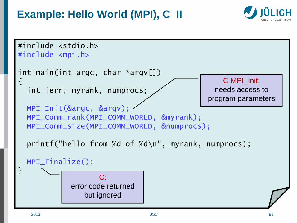
Example: Hello World (MPI), C II
#include <stdio.h> #include <mpi.h> int main(int argc, char *argv[]) { int ierr, myrank, numprocs; MPI_Init(&argc, &argv); MPI_Comm_rank(MPI_COMM_WORLD, &myrank); MPI_Comm_size(MPI_COMM_WORLD, &numprocs); printf("hello from %d of %d\n", myrank, numprocs); MPI_Finalize(); }
C:
error code returned
but ignored
C MPI_Init:
needs access to
program parameters

2013 JSC 92
Compiling MPI Programs
• Many implementations provide special compilation commands
which automatically
direct the compilers to the location of MPI
header files and modules
link in all necessary MPI and network libraries
often called:
C: mpicc
C++: mpiCC, mpicxx, or mpic++
Fortran: mpif90, mpif77

2013 JSC 93
Executing MPI Programs
• Start mechanism is implementation dependent
Many implementations:
mpirun –np <numprocs> <executable> [<options>]
MPI-2 standard:
mpiexec –n <numprocs> <executable> [<options>]
• Possible implementation-dependent differences
Options
Environment variables
Passing runtime parameters, ...
• Start mechanism in general different with a batch system
like PBS (qsub …) or LoadLeveler (llsubmit ...)

2013 JSC 94
Running MPI on Distributed Memory
Interconnect
M0
...
P0
...
myid
numproc
MPI_Init print “hello” MPI_Finalize
Mn
Pn
myid
numproc
MPI_Init print “hello” MPI_Finalize
M1
P1
myid
numproc
MPI_Init print “hello” MPI_Finalize
myid
numproc
MPI_Init print “hello” MPI_Finalize
mpirun

2013 JSC 95
Running MPI on Shared Memory
Interconnect
Memory
P0
...
Pn P1
myid
numproc
MPI_Init print “hello” MPI_Finalize
mpirun MPI_Init print “hello” MPI_Finalize
myid
numproc
MPI_Init print “hello” MPI_Finalize
myid
numproc
MPI_Init print “hello” MPI_Finalize
myid
numproc
2013 JSC 96
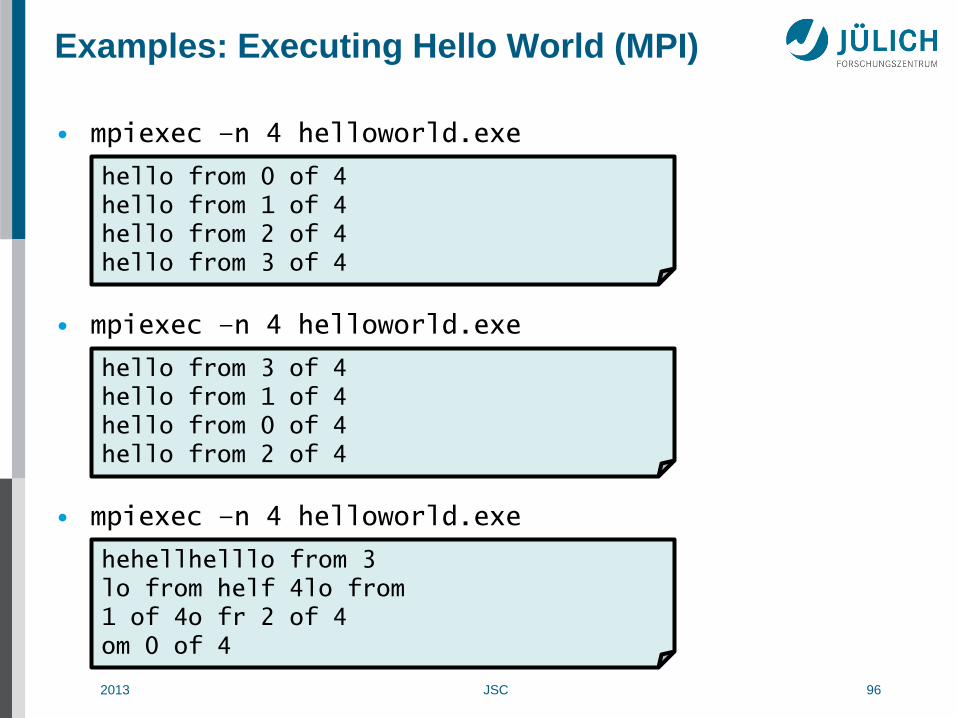
Examples: Executing Hello World (MPI)
• mpiexec –n 4 helloworld.exe
• mpiexec –n 4 helloworld.exe
• mpiexec –n 4 helloworld.exe
hello from 0 of 4 hello from 1 of 4 hello from 2 of 4 hello from 3 of 4
hello from 3 of 4 hello from 1 of 4 hello from 0 of 4 hello from 2 of 4
hehellhelllo from 3 lo from helf 4lo from 1 of 4o fr 2 of 4 om 0 of 4
2013 JSC 97
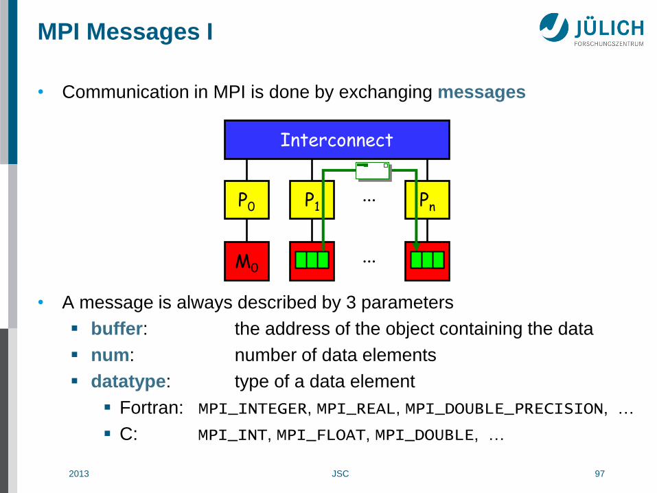
MPI Messages I
• Communication in MPI is done by exchanging messages
• A message is always described by 3 parameters
buffer: the address of the object containing the data
num: number of data elements
datatype: type of a data element
Fortran: MPI_INTEGER, MPI_REAL, MPI_DOUBLE_PRECISION, …
C: MPI_INT, MPI_FLOAT, MPI_DOUBLE, …
P0 P1 Pn ...
Interconnect
M0 ...
2013 JSC 98
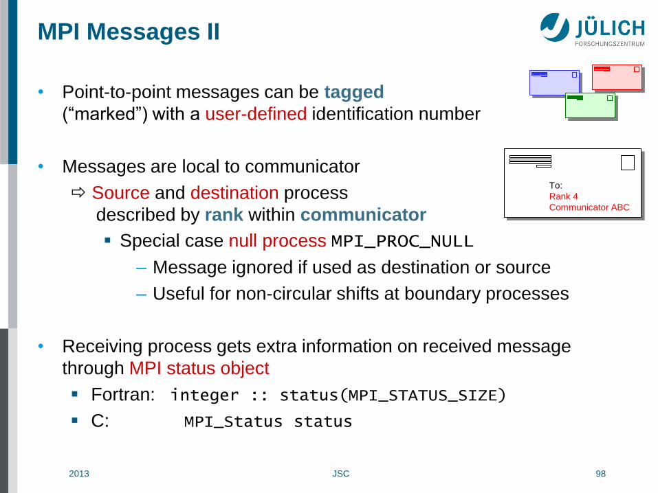
MPI Messages II
• Point-to-point messages can be tagged
(“marked”) with a user-defined identification number
• Messages are local to communicator
Source and destination process
described by rank within communicator
Special case null process MPI_PROC_NULL
– Message ignored if used as destination or source
– Useful for non-circular shifts at boundary processes
• Receiving process gets extra information on received message
through MPI status object
Fortran: integer :: status(MPI_STATUS_SIZE)
C: MPI_Status status
To:
Rank 4
Communicator ABC

2013 JSC 99
Basic MPI Point-to-Point Routines
MPI_Send(buffer, num, datatype, dest, tag, comm)
Called on sender process
Pack data inside buffer into a message tagged with tag and
send it out to rank dest within comm
MPI_Recv(buffer, num, datatype, src, tag, comm, status)
Called on receiver process
Receive message tagged with tag from rank src within comm and unpack message into data buffer
MPI_Sendrecv(sendbuf, sendnum, senddtype, dest, sendtag,
recvbuf, recvnum, recvdtype, src, recvtag,
comm, status)
Send a message and receive one at the same time
Useful for executing shift across a chain of processes

2013 JSC 100
Example:
Sending Messages in a Ring, Fortran
program shift include 'mpif.h' integer :: left, right, ierr, myrank, numprocs integer :: value=0, tag=42, status(MPI_STATUS_SIZE) call MPI_Init(ierr) call MPI_Comm_rank(MPI_COMM_WORLD, myrank, ierr) call MPI_Comm_size(MPI_COMM_WORLD, numprocs, ierr) left = mod(myrank - 1 + numprocs, numprocs) right = mod(myrank + 1, numprocs) call MPI_Sendrecv(myrank, 1, MPI_INTEGER, right, tag, & value, 1, MPI_INTEGER, left, tag, & MPI_COMM_WORLD, status, ierr) write (*,*) myrank, "received", value call MPI_Finalize(ierr) end program

2013 JSC 101
Example:
Sending Messages in a Ring, C
#include <stdio.h> #include <mpi.h> int main(int argc, char* argv[]) { int left, right, ierr, myrank, numprocs, value=0, tag=42; MPI_Status status; MPI_Init(&argc, &argv); MPI_Comm_rank(MPI_COMM_WORLD, &myrank); MPI_Comm_size(MPI_COMM_WORLD, &numprocs); left = (myrank - 1 + numprocs) % numprocs; right = (myrank + 1) % numprocs; MPI_Sendrecv(&myrank, 1, MPI_INT, right, tag, &value, 1, MPI_INT, left, tag, MPI_COMM_WORLD, &status); printf("%d received %d\n", myrank, value); MPI_Finalize(); return 0; }
2013 JSC 102
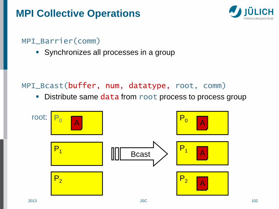
MPI Collective Operations
MPI_Barrier(comm)
Synchronizes all processes in a group
MPI_Bcast(buffer, num, datatype, root, comm)
Distribute same data from root process to process group
P0 A
P1
P2
P0 A
P1
P2
Bcast
root:
A
A
2013 JSC 103
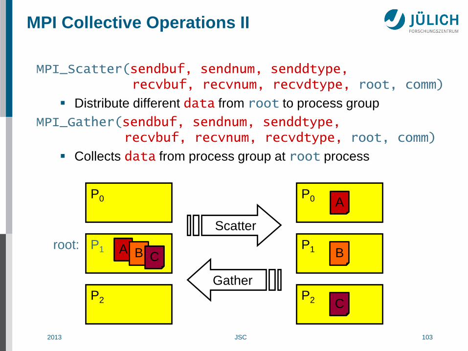
MPI Collective Operations II
MPI_Scatter(sendbuf, sendnum, senddtype, recvbuf, recvnum, recvdtype, root, comm)
Distribute different data from root to process group
MPI_Gather(sendbuf, sendnum, senddtype, recvbuf, recvnum, recvdtype, root, comm)
Collects data from process group at root process
P0
P1
P2
P0 A
P1
P2 C
B
Scatter
Gather
root: A B C
2013 JSC 104
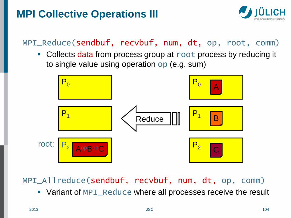
MPI Collective Operations III
MPI_Reduce(sendbuf, recvbuf, num, dt, op, root, comm)
Collects data from process group at root process by reducing it
to single value using operation op (e.g. sum)
MPI_Allreduce(sendbuf, recvbuf, num, dt, op, comm)
Variant of MPI_Reduce where all processes receive the result
P0
P1
P2
P0 A
P1
P2 C
B Reduce
root: AopBopC

2013 JSC 105
Example: Max value of Polynomial (serial)
program poly_max_serial integer :: i,nsteps double precision :: x,y,ymax,step,coeff(4),xmin,xmax open(1, file="poly.dat") read(1,*) coeff, xmin, xmax, nsteps ymax = -huge(x) x = xmin step = (xmax - xmin) / (nsteps - 1) do i = 1, nsteps y = coeff(4)*x**3 + coeff(3)*x**2 + coeff(2)*x + coeff(1) ymax = max(ymax, y) x = x + step end do write(*,*) "Maximum is ", ymax end program

2013 JSC 106
MPI Work Distribution
do i = 1, N call work(i) end do
do i = rank+1, N, numprocs call work(i) end do
Cyclic
c = N / numprocs low = rank*c + 1 high = low + c – 1 if (rank==numprocs-1) & high = N do i = low, high call work(i) end do
Block 0 1 2 3 4 5 6 7 8 9
c = N / numprocs r = mod(N,numprocs) low = rank*c + min(rank,r) + 1 if (rank<r) c = c + 1 high = low + c - 1 do i = low, high call work(i) end do
Block balanced 0 1 2 3 4 5 6 7 8 9
0 1 2 3 4 5 6 7 8 9 Sequential 0
2013 JSC 107
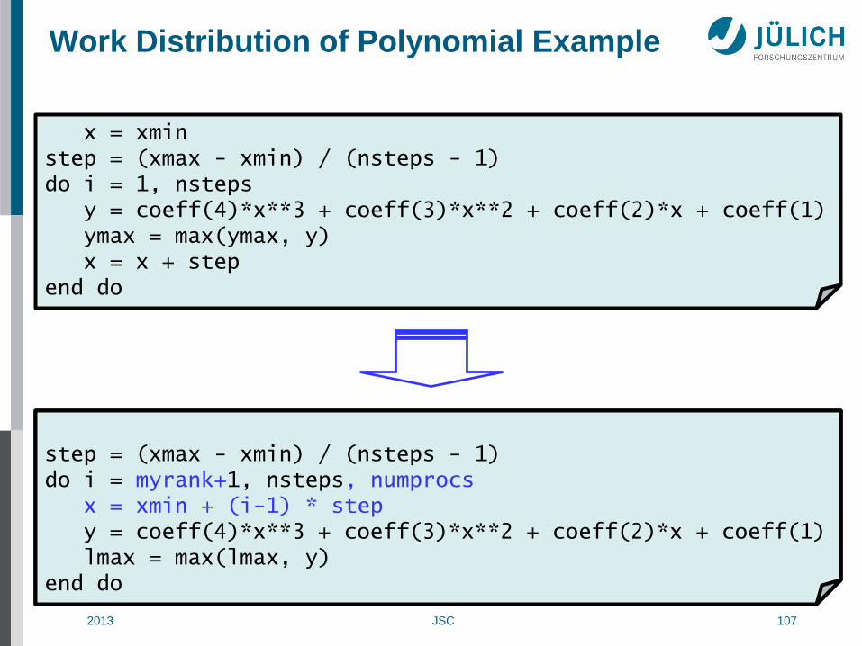
Work Distribution of Polynomial Example
x = xmin step = (xmax - xmin) / (nsteps - 1) do i = 1, nsteps y = coeff(4)*x**3 + coeff(3)*x**2 + coeff(2)*x + coeff(1) ymax = max(ymax, y) x = x + step end do
x = xmin step = (xmax - xmin) / (nsteps - 1) do i = myrank+1, nsteps, numprocs y = coeff(4)*x**3 + coeff(3)*x**2 + coeff(2)*x + coeff(1) ymax = max(ymax, y) x = x + step end do
x = xmin step = (xmax - xmin) / (nsteps - 1) do i = myrank+1, nsteps, numprocs y = coeff(4)*x**3 + coeff(3)*x**2 + coeff(2)*x + coeff(1) ymax = max(ymax, y) x = x + step end do
step = (xmax - xmin) / (nsteps - 1) do i = myrank+1, nsteps, numprocs x = xmin + (i-1) * step y = coeff(4)*x**3 + coeff(3)*x**2 + coeff(2)*x + coeff(1) lmax = max(lmax, y) end do

2013 JSC 108
Example: Max value of Polynomial (MPI) I
program poly_max_mpi include 'mpif.h' integer :: i,ierr,myrank,numprocs double precision :: x,y,ymax,lmax,step,coeff(4),domain(3) call MPI_Init(ierr) call MPI_Comm_rank(MPI_COMM_WORLD, myrank, ierr) call MPI_Comm_size(MPI_COMM_WORLD, numprocs, ierr) if ( myrank == 0 ) then open(1, file="poly.dat") read(1,*) coeff, domain endif call MPI_Bcast(coeff, 4, MPI_DOUBLE_PRECISION, 0, & MPI_COMM_WORLD, ierr) call MPI_Bcast(domain, 3, MPI_DOUBLE_PRECISION, 0, & MPI_COMM_WORLD, ierr)
2013 JSC 109
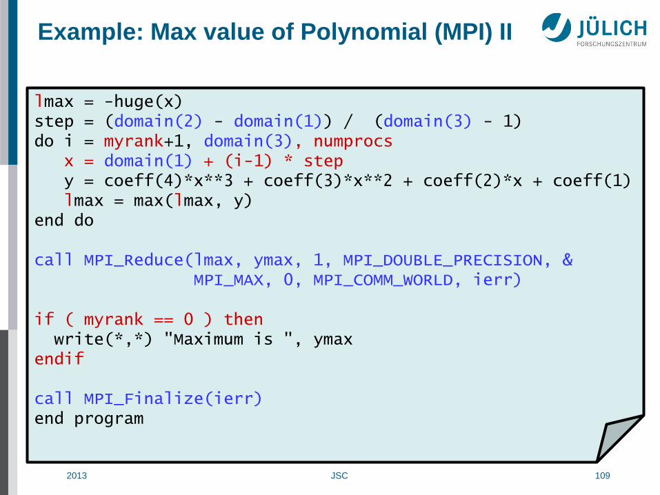
Example: Max value of Polynomial (MPI) II
lmax = -huge(x) step = (domain(2) - domain(1)) / (domain(3) - 1) do i = myrank+1, domain(3), numprocs x = domain(1) + (i-1) * step y = coeff(4)*x**3 + coeff(3)*x**2 + coeff(2)*x + coeff(1) lmax = max(lmax, y) end do call MPI_Reduce(lmax, ymax, 1, MPI_DOUBLE_PRECISION, & MPI_MAX, 0, MPI_COMM_WORLD, ierr) if ( myrank == 0 ) then write(*,*) "Maximum is ", ymax endif call MPI_Finalize(ierr) end program

2013 JSC 110
Example:
PI Calculation (serial)
program pi_serial ! Approximate with integer :: i,n ! n-point rectangle double precision :: x,sum,pi,h ! quadrature rule open(1, file="pi.dat") read(1,*) n ! Number of rectangles h = 1.0d0 / n sum = 0.0d0 do i = 1, n x = (i - 0.5d0)*h sum = sum + (4.d0/(1.d0 + x*x)) end do pi = h * sum write(*, fmt="(A, F16.12)") "Value of pi is ", pi end program

2013 JSC 111
Example:
PI Calculation (MPI) I
program pi_mpi include 'mpif.h' integer :: i,n,ierr,myrank,numprocs double precision :: x,sum,pi,h,mypi call MPI_Init(ierr) call MPI_Comm_rank(MPI_COMM_WORLD, myrank, ierr) call MPI_Comm_size(MPI_COMM_WORLD, numprocs, ierr) if ( myrank == 0 ) then open(1, file="pi.dat") read(1,*) n end if call MPI_Bcast(n, 1, MPI_INTEGER, 0, MPI_COMM_WORLD, ierr) ...
2013 JSC 112
Example:
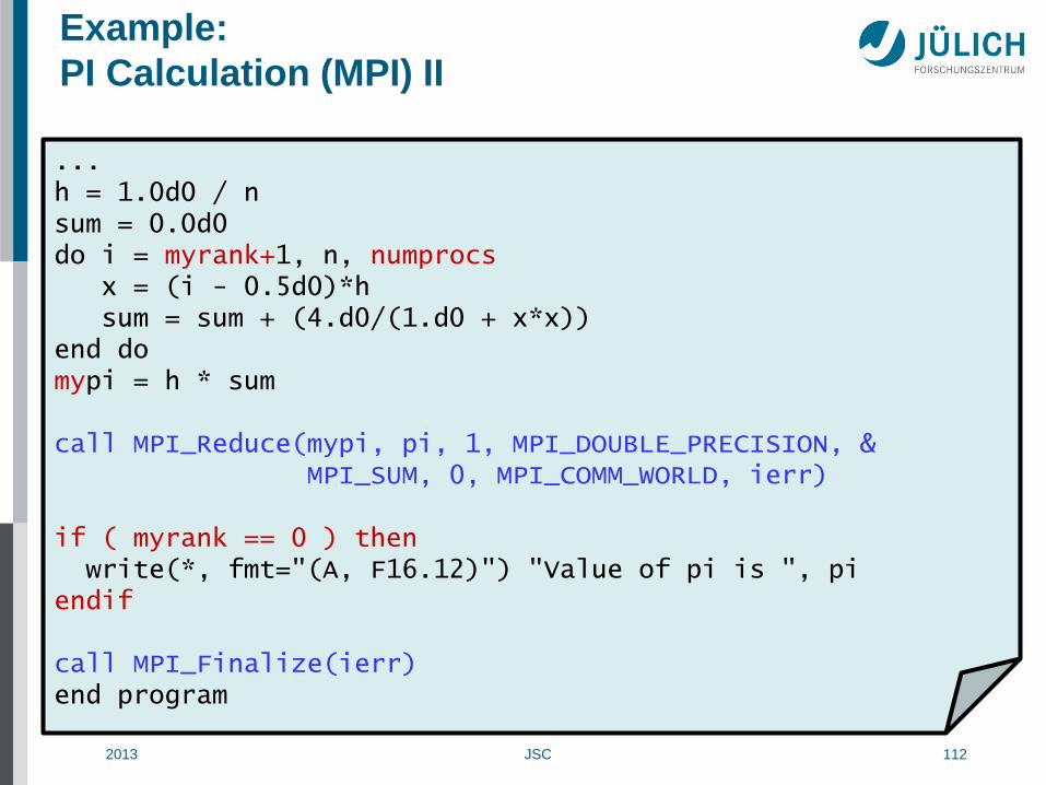
PI Calculation (MPI) II
... h = 1.0d0 / n sum = 0.0d0 do i = myrank+1, n, numprocs x = (i - 0.5d0)*h sum = sum + (4.d0/(1.d0 + x*x)) end do mypi = h * sum call MPI_Reduce(mypi, pi, 1, MPI_DOUBLE_PRECISION, & MPI_SUM, 0, MPI_COMM_WORLD, ierr) if ( myrank == 0 ) then write(*, fmt="(A, F16.12)") "Value of pi is ", pi endif call MPI_Finalize(ierr) end program

2013 JSC 113
MPI Evaluation
• Advantages
Supplies communication, synchronization, and I/O variations and
optimized functions for a wide range of needs
Supported by all major parallel computer vendors;
optimized for the vendor’s hardware
Free open-source versions available (MPICH, OpenMPI,…)
About 130 functions (MPI 1), now 320 functions (MPI 2)
But basic programs can be implemented with 10 to 20 functions
gentle learning curve
• Disadvantages
High programming overhead
explicit data distribution, communication, and synchronization
Separate sequential and parallel version of program necessary
MPI codes help preserve your investment as systems change!
2013 JSC 114
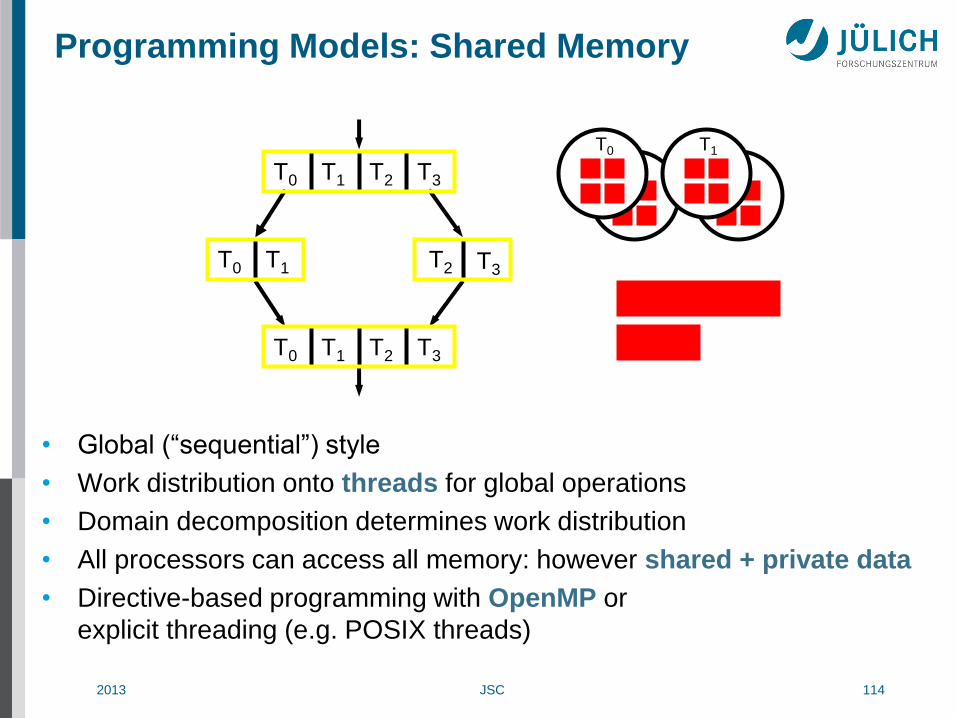
Programming Models: Shared Memory
• Global (“sequential”) style
• Work distribution onto threads for global operations
• Domain decomposition determines work distribution
• All processors can access all memory: however shared + private data
• Directive-based programming with OpenMP or
explicit threading (e.g. POSIX threads)
T2 T3 T0 T1 T2 T3
T2 T3 T0 T1
T0 T1 T2 T3
T0 T1
2013 JSC 115
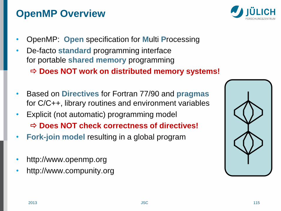
OpenMP Overview
• OpenMP: Open specification for Multi Processing
• De-facto standard programming interface
for portable shared memory programming
Does NOT work on distributed memory systems!
• Based on Directives for Fortran 77/90 and pragmas
for C/C++, library routines and environment variables
• Explicit (not automatic) programming model
Does NOT check correctness of directives!
• Fork-join model resulting in a global program
• http://www.openmp.org
• http://www.compunity.org
2013 JSC 116
History
• Proprietary designs by some vendors (SGI, CRAY, SUN, IBM, …)
end of the 1980’s
• Different unsuccessful attempts to standardize API
PCF
ANSI X3H5
• OpenMP-Forum founded to define portable API
1997 first API for Fortran (V1.0)
1998 first API for C/C++ (V1.0)
2000 Fortran V2.0
2002 C/C++ V2.0
2005 combined C/C++/Fortran specification V2.5
2008 V3.0
2011 V3.1

2013 JSC 117
OpenMP Functionality
• Directives/pragmas
Parallel regions (execute the same code in parallel)
Parallel loops (execute loop iterations in parallel)
Parallel sections (execute different sections in parallel)
Tasks (dynamically create and execute tasks in parallel, since V3.0)
Execution by exactly one single or master thread
Shared and private data
Reductions
Synchronization primitives (Barrier, Critical region, Atomic)
• Run-time library functions
omp_get_num_threads(), omp_get_thread_num()
omp_set_lock(), omp_unset_lock(), …
• Environment variables
OMP_NUM_THREADS, …

2013 JSC 118
OpenMP Execution Model
a = 1 a = 2 do i = 1,9 call work(i) enddo a = 3
Program:
Thread0
(Sequential) Execution:
a = 1 a = 2 i=1..9: work(i) enddo a = 3

2013 JSC 119
OpenMP Execution Model
a = 1 !$omp parallel a = 2 do i = 1,9 call work(i) enddo !$omp end parallel a = 3
Program:
Thread0 Thread1 Thread2
(Parallel) Execution:
a = 1 a = 2 a = 2 a = 2 i=1..9: i=1..9: i=1..9: work(i) work(i) work(i) enddo enddo enddo a = 3
parallel region

2013 JSC 120
OpenMP Execution Model
a = 1 !$omp parallel a = 2 !$omp do do i = 1,9 call work(i) enddo !$omp end parallel a = 3
Program: (Parallel) Execution:
a = 1 a = 2 a = 2 a = 2 i=1..3: i=4..6: i=7..9: work(i) work(i) work(i) enddo enddo enddo a = 3
Thread0 Thread1 Thread2
parallel region
parallel loop

2013 JSC 121
Example: Hello World (OpenMP), Fortran
program main integer :: myid, nthreads integer :: OMP_Get_num_threads, OMP_Get_thread_num !$omp parallel private(myid, nthreads) myid = OMP_Get_thread_num() nthreads = OMP_Get_num_threads() write(*,*) "hello from", myid, "of", nthreads !$omp end parallel end program

2013 JSC 122
Example: Hello World (OpenMP), C
#include <stdio.h> #include <omp.h> int main() { int myid, nthreads; #pragma omp parallel private(myid, nthreads) { myid = omp_get_thread_num(); nthreads = omp_get_num_threads(); printf("hello from %d of %d\n", myid, nthreads); } }

2013 JSC 123
OpenMP 3.0 – Introducing Tasks
• Tasks describe independent chunks of work
• Useful for:
Tree traversals
Linked lists
Recursive algorithms
• Basic usage (C):
void process_leaf(int nodeID) { ... #pragma omp task { process_leaf( left_childID[ nodeID ] ); } ... }
2013 JSC 124
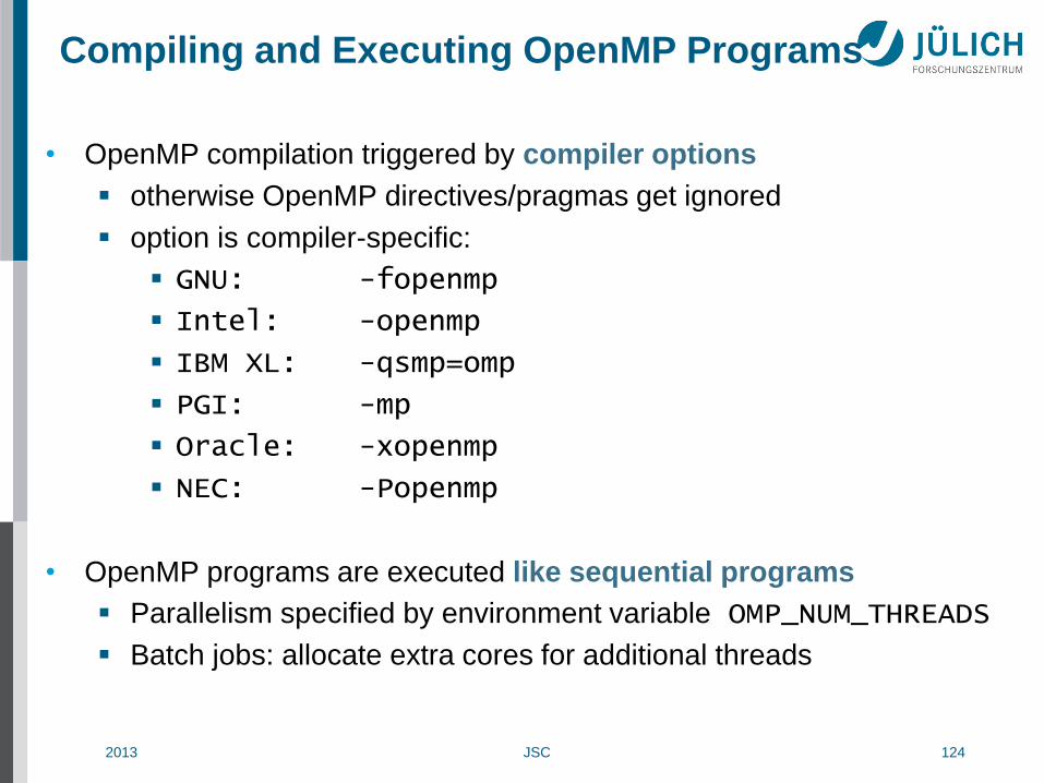
Compiling and Executing OpenMP Programs
• OpenMP compilation triggered by compiler options
otherwise OpenMP directives/pragmas get ignored
option is compiler-specific:
GNU: -fopenmp
Intel: -openmp
IBM XL: -qsmp=omp
PGI: -mp
Oracle: -xopenmp
NEC: -Popenmp
• OpenMP programs are executed like sequential programs
Parallelism specified by environment variable OMP_NUM_THREADS
Batch jobs: allocate extra cores for additional threads
2013 JSC 125
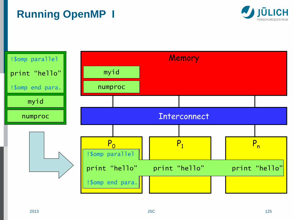
Running OpenMP I
Interconnect
Memory
P0
...
Pn P1
myid
numproc
!$omp parallel
print “hello” !$omp end para.
myid
numproc
!$omp parallel
print “hello” !$omp end para.
!$omp parallel
print “hello” print “hello” print “hello” !$omp end para.
2013 JSC 126
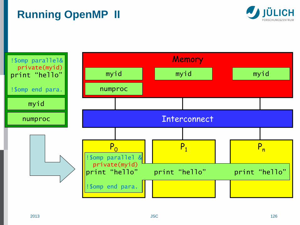
Running OpenMP II
Interconnect
Memory
P0
...
Pn P1
myid
numproc
!$omp parallel& private(myid)
print “hello” !$omp end para.
myid
numproc
!$omp parallel& private(myid)
print “hello” !$omp end para.
!$omp parallel & private(myid)
print “hello” print “hello” print “hello” !$omp end para.
myid myid

2013 JSC 127
Example: Max value of Polynomial (OpenMP)
program poly_max_omp integer :: i,nsteps double precision :: x,y,ymax,step,coeff(4),xmin,xmax open(1, file="poly.dat") read(1,*) coeff, xmin, xmax, nsteps ymax = -huge(x) step = (xmax - xmin) / (nsteps - 1) !$omp parallel do private(x,y) reduction(max:ymax) do i = 1, nsteps x = xmin + (i-1) * step y = coeff(4)*x**3 + coeff(3)*x**2 + coeff(2)*x + coeff(1) ymax = max(ymax, y) end do write(*,*) "Maximum is ", ymax end program

2013 JSC 128
Example:
PI Calculation (OpenMP)
program pi_omp integer :: i,n double precision :: x,sum,pi,h open(1, file="pi.dat") read(1,*) n h = 1.0d0 / n sum = 0.0d0 !$omp parallel do private(x) reduction(+:sum) do i = 1, n x = (i - 0.5d0)*h sum = sum + (4.d0/(1.d0 + x*x)) end do pi = h * sum write(*, fmt="(A, F16.12)") "Value of pi is ", pi end program

2013 JSC 129
OpenMP Work Distribution
• OpenMP also provides:
schedule(dynamic [, chunk])
schedule(guided [, chunk])
do i = 1, N call work(i) end do
!$omp do schedule(static,1) do i = 1, N call work(i) end do
Cyclic 0 1 2 3 4 5 6 7 8 9 Sequential 0
0 1 2 3 4 5 6 7 8 9
0 1 2 3 4 5 6 7 8 9
!$omp do schedule(static) do i = 1, N call work(i) end do
Block ?
2013 JSC 130
OpenMP Evaluation
• Advantages
Stable standard
Supported by all major parallel computer + compiler vendors;
optimized for the vendor’s hardware
Lean: simple and limited set of compiler directives
Ease of use
supports incremental parallelization
Sequential version = parallel version
• Disadvantages
Only works on shared memory machines
Requires special compiler
GNU OpenMP since V4.2
Danger of missing or incorrect synchronization
Getting efficient parallel implementation often hard
2013 JSC 131
Low-Level GPGPU Programming
• Proprietary programming languages or extensions
NVIDIA: CUDA (C/C++ based)
AMD: StreamSDK or Brooks+ (C/C++ based)
• OpenCL (Open Computing Language)
Open standard for portable, parallel programming
of heterogeneous parallel computing
CPUs, GPUs, and other processors
• Major rewriting of the code required, not portable
Best performance, usually only needed for
Important kernels
Libraries
2013 JSC 132
High-Level GPGPU Programming
• Compilation systems with
(OpenMP-like) directives for GPU programming
User tells compiler which part of code to accelerate
Portland Group Fortran and C compilers
http://www.pgroup.com/resources/accel.htm
CAPS HMPP (Fortran, C)
http://www.caps-enterprise.com/hmpp.html
OpenACC joint-venture by:
NVIDIA
Portland Group
CRAY
CAPS
http://www.openacc-standard.org
2013 JSC 133
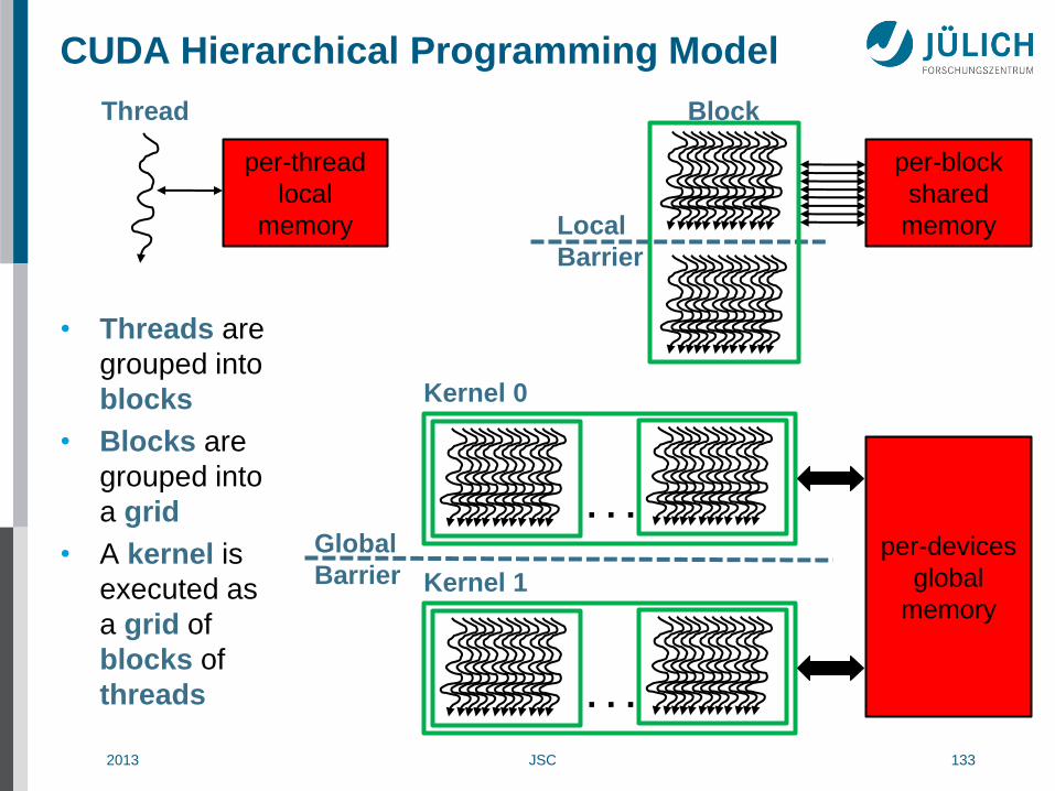
CUDA Hierarchical Programming Model
• Threads are
grouped into
blocks
• Blocks are
grouped into
a grid
• A kernel is
executed as
a grid of
blocks of
threads
Thread
per-thread
local
memory
Block
Local
Barrier
per-block
shared
memory
Kernel 0
. . . Global
Barrier Kernel 1
. . .
per-devices
global
memory

2013 JSC 134
EXAMPLE: CUDA saxpy Code
/* -- Sequential Version -------------------------------- */ void saxpy_s(int n, float a, float x[], float y[]) { for (int i=0; i<n; ++i) y[i] = a * x[i] + y[i]; } saxpy_s(n, 2.0, x, y); /* -- CUDA Parallel Version ----------------------------- */ __global__ void saxpy_p(int n, float a, float x[], float y[]) { int i = blockIdx.x * blockDim.x + threadIdx.x; if (i < n) y[i] = a * x[i] + y[i]; } /* -- Invoke kernel with 256 threads/block int nblocks = (n + 255) / 256; saxpy_p<<<nblocks, 256>>>(n, 2.0, x, y);
2013 JSC 135
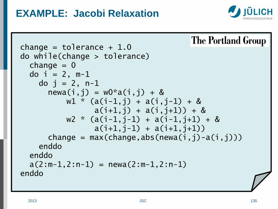
EXAMPLE: Jacobi Relaxation
change = tolerance + 1.0 do while(change > tolerance) change = 0 do i = 2, m-1 do j = 2, n-1 newa(i,j) = w0*a(i,j) + & w1 * (a(i-1,j) + a(i,j-1) + & a(i+1,j) + a(i,j+1)) + & w2 * (a(i-1,j-1) + a(i-1,j+1) + & a(i+1,j-1) + a(i+1,j+1)) change = max(change,abs(newa(i,j)-a(i,j))) enddo enddo a(2:m-1,2:n-1) = newa(2:m-1,2:n-1) enddo

2013 JSC 136
EXAMPLE: Device-side CUDA C Kernel Ia
extern "C" __global__ void jacobikernel( float* a, float* anew, float* lchange, int n, int m ) { int ti = threadIdx.x, tj = threadIdx.y; /* local indices */ int i = blockIdx.x*16+ti; /* global indices */ int j = blockIdx.y*16+tj; __shared__ float mychange[16*16], b[18][18]; b[tj][ti] = a[(j-1)*m+i-1]; if(i<2) b[tj][ti+16] = a[(j-1)*m+i+15]; if(j<2) b[tj+16][ti] = a[(j+15)*m+i-1]; if(i<2&&j<2) b[tj+16][ti+16] = a[(j+15)*m+i+15]; __syncthreads(); mya = w0 * b[tj+1][ti+1] + w1 * (b[tj+1][ti] + b[tj][ti+1] + b[tj+1][ti+2] + b[tj+2][ti+1]) + w2 * (b[tj][ti] + b[tj+2][ti] + b[tj][ti+2] + b[tj+2][ti+2]); newa[j][i] = mya;

2013 JSC 137
EXAMPLE: Device-side CUDA C Kernel Ib
/* this thread's "change" */ mychange[ti+16*tj] = fabs(mya,b[tj+1][ti+2]); __syncthreads(); /* reduce all "change" values for this thread block * to a single value */ n = 256; while( n <<= 1 ){ if( tx+ty*16 < n ) mychange[ti+tj*16] = fmaxf( mychange[ti+tj*16], mychange[ti+tj*16+n]); __syncthreads(); } /* store this thread block's "change" */ if(tx==0&&ty==0) lchange[blockIdx.x+blockDim.x*blockIdx.y] = mychange[0]; }

2013 JSC 138
EXAMPLE: Device-side CUDA C Kernel II
/*reduce all thread block's "change" values*/ extern “C” __global__ void reduction( float* lchange, int n ) { __shared__ float mychange[256]; float mych = lchange[i]; int i = threadIdx.x, m = n; while( m <= n ){ mych = fmaxf(mych,lchange[m]); m += n; } mychange[i] = mych; __syncthreads(); n = 256; while( n <<= 1 ){ if(i<n) mychange[i] = fmaxf(mychange[i],mychange[i+n]); __syncthreads(); } if(i==0) change = mychange[0]; }

2013 JSC 139
EXAMPLE: Device-side CUDA C Kernel III
/* Update 'a' from 'newa */ extern "C" __global__ void updatekernel( float* a, float* anew, int n, int m ) { int i = blockIdx.x*16 + threadIdx.x; int j = blockIdx.y*16 + threadIdx.y; a[j*m+i] = newa[j*m+i]; }
2013 JSC 140
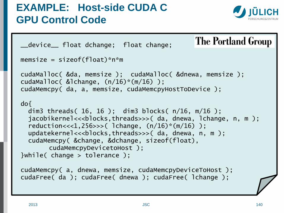
EXAMPLE: Host-side CUDA C
GPU Control Code
__device__ float dchange; float change; memsize = sizeof(float)*n*m cudaMalloc( &da, memsize ); cudaMalloc( &dnewa, memsize ); cudaMalloc( &lchange, (n/16)*(m/16) ); cudaMemcpy( da, a, memsize, cudaMemcpyHostToDevice ); do{ dim3 threads( 16, 16 ); dim3 blocks( n/16, m/16 ); jacobikernel<<<blocks,threads>>>( da, dnewa, lchange, n, m ); reduction<<<1,256>>>( lchange, (n/16)*(m/16) ); updatekernel<<<blocks,threads>>>( da, dnewa, n, m ); cudaMemcpy( &change, &dchange, sizeof(float), cudaMemcpyDevicetoHost ); }while( change > tolerance ); cudaMemcpy( a, dnewa, memsize, cudaMemcpyDeviceToHost ); cudaFree( da ); cudaFree( dnewa ); cudaFree( lchange );
2013 JSC 141
OpenACC
• High-level programming model, similar to OpenMP
• Joint-venture to develop an open, portable standard
• All members are part of the OpenMP language committee
• Compilers have preliminary support, full support announced for
Q4/2012
• Tuning is done by specifying data regions for which data:
Can reside on the GPU over several iterations
Can be shared between different loop regions
Is only needed locally on the GPU
• Compiler developers focus on implementing good optimization
schemes themselves
2013 JSC 142
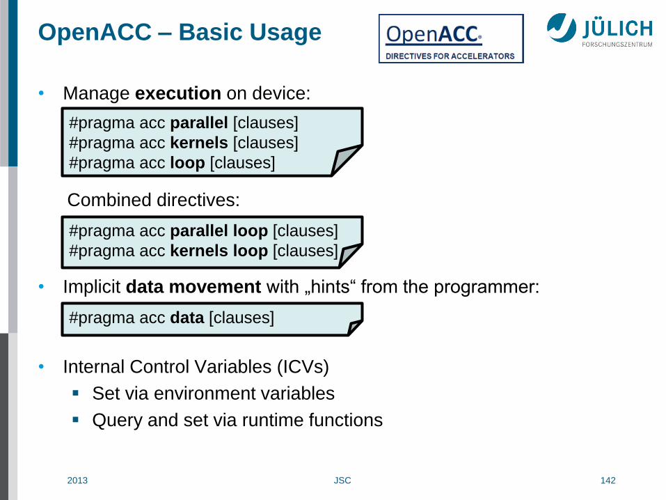
OpenACC – Basic Usage
• Manage execution on device:
Combined directives:
• Implicit data movement with „hints“ from the programmer:
• Internal Control Variables (ICVs)
Set via environment variables
Query and set via runtime functions
#pragma acc parallel [clauses]
#pragma acc kernels [clauses]
#pragma acc loop [clauses]
#pragma acc data [clauses]
#pragma acc parallel loop [clauses]
#pragma acc kernels loop [clauses]
2013 JSC 143
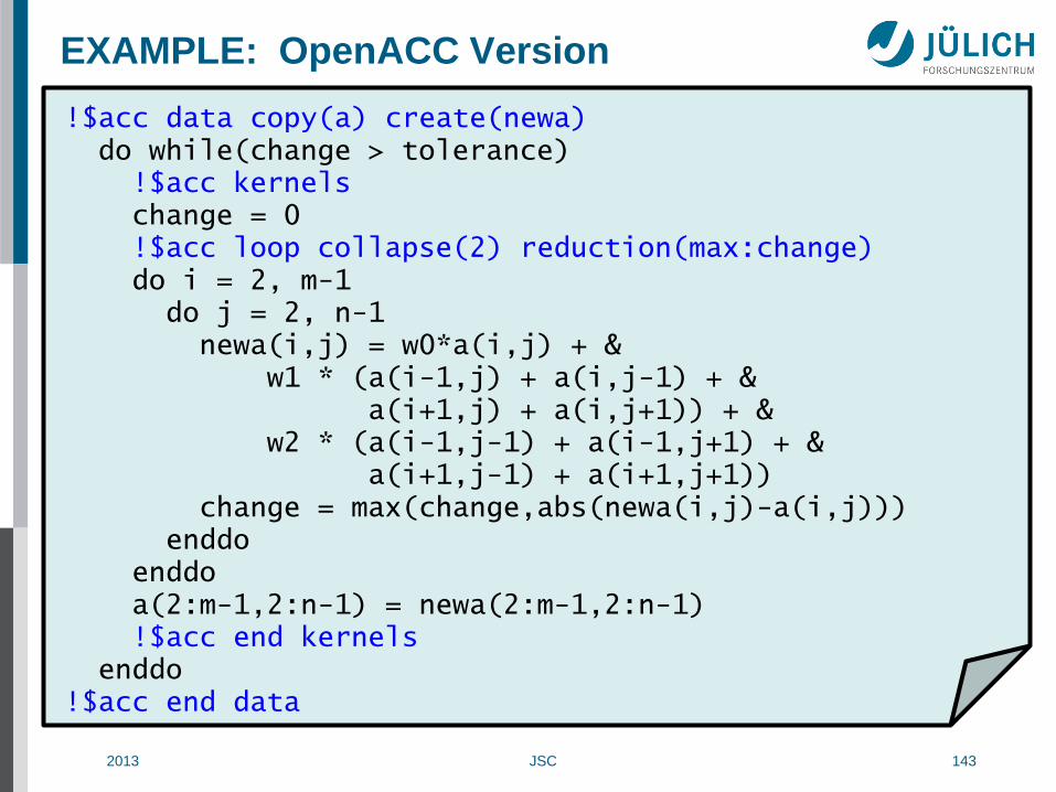
EXAMPLE: OpenACC Version
!$acc data copy(a) create(newa) do while(change > tolerance) !$acc kernels change = 0 !$acc loop collapse(2) reduction(max:change) do i = 2, m-1 do j = 2, n-1 newa(i,j) = w0*a(i,j) + & w1 * (a(i-1,j) + a(i,j-1) + & a(i+1,j) + a(i,j+1)) + & w2 * (a(i-1,j-1) + a(i-1,j+1) + & a(i+1,j-1) + a(i+1,j+1)) change = max(change,abs(newa(i,j)-a(i,j))) enddo enddo a(2:m-1,2:n-1) = newa(2:m-1,2:n-1) !$acc end kernels enddo !$acc end data

2013 JSC 144
CAPS HMPP Directives
• Codelet is a pure function that can be remotely executed on a GPU
• Regions are a short cut
for writing codelets
• Target clause specifies what
GPU code to generate
GPU can be CUDA or OpenCL
The runtime selects out of the available hardware and code
• Parallel loops are the code constructs converted in GPU threads
Directive hmppcg parallel forces parallelization
Two levels of parallelism can be used to generate the threads
#pragma hmpp myfunc codelet, target=GPU, … void saxpy(int n, float alpha, float x[n], float y[n]){ #pragma hmppcg parallel for(int i = 0; i<n; ++i) y[i] = alpha*x[i] + y[i]; }
#pragma hmpp myreg region, … { for(int i = 0; i<n; ++i) y[i] = alpha*x[i] + y[i]; }
2013 JSC 145
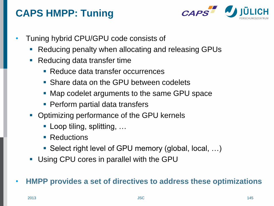
CAPS HMPP: Tuning
• Tuning hybrid CPU/GPU code consists of
Reducing penalty when allocating and releasing GPUs
Reducing data transfer time
Reduce data transfer occurrences
Share data on the GPU between codelets
Map codelet arguments to the same GPU space
Perform partial data transfers
Optimizing performance of the GPU kernels
Loop tiling, splitting, …
Reductions
Select right level of GPU memory (global, local, …)
Using CPU cores in parallel with the GPU
• HMPP provides a set of directives to address these optimizations

2013 JSC 146
Advantages of Pragma/directives-based
GPU Programming
• "Only" need to add pragmas/directives
Single Code for "normal" and accelerated version
Incremental program migration
Minimal code changes
• Auto-generated
Data allocation and transfers
Reductions
(Partially) Heuristics for thread block size and shape
• "Standard" tool chain
• Potential for future portability

2013 JSC 147
Dual Level Parallelism
• Often: Applications have two natural levels of parallelism.
If possible, take advantage of it and exploit by using OpenMP
within an SMP node and by using MPI between nodes
• Why ?
MPI performance degrades when
Domains become too small
Message latency dominates computation
Parallelism is exhausted
OpenMP
Typically has lower latency
Can maintain speedup at finer granularity
• Drawback:
Programmer must know MPI and OpenMP
Code might be harder to debug, analyze and maintain

2013 JSC 148
Hybrid Programming
• Many of today’s most powerful computers employ both shared memory
and distributed memory architectures
hybrid systems
• The corresponding hybrid programming model is a combination of
shared and distributed memory programming
MPI and OpenMP
MPI and POSIX threads
MPI and multi-threaded libraries
• Can give better scalability than pure MPI or OpenMP
• Upcoming systems with accelerators complicate the situation:
Hybrid programming will become the norm:
Multi-threaded + accelerators
MPI + multi-threaded + accelerators

2013 JSC 149
Intel MIC Programming
• Based on “standard” programming models
MPI, OpenMP, or MPI/OpenMP
On a set of MIC nodes
On a set of Cluster and MIC nodes
• Using offload directives (probably in OpenMP V4)
MPI program on Cluster nodes
Offloading (OpenMP) kernels to MIC nodes
• Various Intel proprietary programming models
Cilk Plus
TBB
OpenCL
…

2013 JSC 150
DEBUGGING AND
PERFORMANCE ANALYSIS

2013 JSC 151
Performance Properties of Parallel Programs
• Factors which influence performance of parallel programs
“Sequential” factors
Computation
Cache and memory
Input / output
“Parallel” factors
Communication (Message passing)
Threading
Synchronization
Accelerators
Choose right algorithm, use optimizing compiler
Tough! Not many tools yet, hope compiler gets it right
Not given enough attention
More or less understood, tool support
Tough! Very little, simple tools for now

2013 JSC 152
Metrics of Performance
• What can be measured?
A count of how many times an event occurs
The duration of some time interval
The size of some parameter
• Derived metrics (e.g., rates) needed for normalization
• Typical metrics
Execution time
MIPS
Millions of instructions
executed per second
MFLOPS/GFLOPS
Millions/billions of floating-point operations per second
Cache or TLB misses
…
“math” Operations?
HW Operations?
HW Instructions?
32-/64-bit? …

2013 JSC 153
Example: Time Measurement (MPI)
program main include 'mpif.h' integer :: ierr, myrank, numprocs double precision :: starttime, endtime !double in C/C++ call MPI_Init(ierr) call MPI_Comm_rank(MPI_COMM_WORLD, myrank, ierr) call MPI_Comm_size(MPI_COMM_WORLD, numprocs, ierr) starttime = MPI_Wtime() write(*,*) "hello from", myrank, "of", numprocs endtime = MPI_Wtime() write(*,*) myrank, "used", endtime-starttime, "seconds" call MPI_Finalize(ierr) end program

2013 JSC 154
Example: Time Measurement (OpenMP)
program main integer :: myid, nthreads integer :: OMP_Get_num_threads, OMP_Get_thread_num double precision :: OMP_Get_wtime, starttime, endtime starttime = OMP_Get_wtime() !$omp parallel private(myid) myid = OMP_Get_thread_num() nthreads = OMP_Get_num_threads() write(*,*) "hello from", myid, "of", nthreads !$omp end parallel endtime = OMP_Get_wtime() write(*,*)"used", endtime-starttime, "seconds" end program
2013 JSC 155
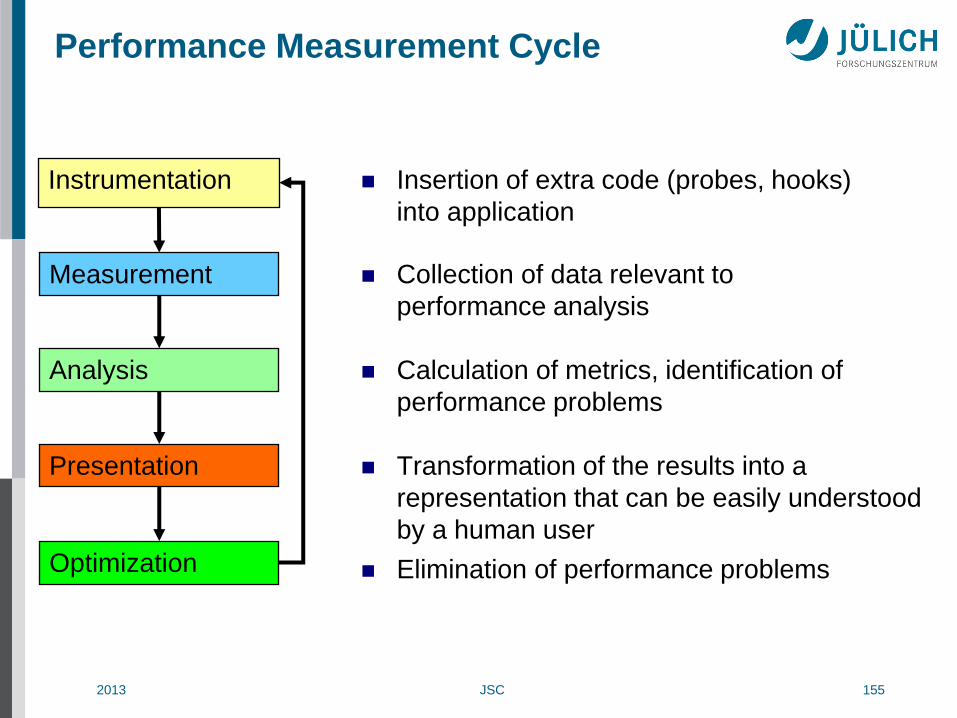
Performance Measurement Cycle
Insertion of extra code (probes, hooks)
into application
Instrumentation
Transformation of the results into a
representation that can be easily understood
by a human user
Presentation
Measurement Collection of data relevant to
performance analysis
Optimization Elimination of performance problems
Analysis Calculation of metrics, identification of
performance problems
2013 JSC 156
Performance Measurement
• Two dimensions
When performance measurement is triggered
Externally (asynchronous) indirect measurement
– Sampling
» Timer interrupt
» Hardware counters overflow
Internally (synchronous) direct measurement
– Code instrumentation
» Automatic or manual instrumentation
How performance data is recorded
Profile ::= Summation of events over time
– run time summarization (functions, call sites, loops, …)
Trace file ::= Sequence of events over time
2013 JSC 157
Measurement Methods: Profiling I
• Recording of aggregated information
Time
Counts
Calls
Hardware counters
• about program and system entities
Functions, call sites, loops, basic blocks, …
Processes, threads
• Statistical information: min, max, mean and total number of values
• Methods to create a profile
PC sampling (statistical approach)
Interval timer / direct measurement (deterministic approach)
2013 JSC 158
Profiling II
• Sampling
General statistical measurement technique based on the assumption that a subset of a population being examined is representative for the whole population
Running program is interrupted periodically
Operating system signal or Hardware counter overflow
Interrupt service routine examines return-address stack to find address of instruction being executed when interrupt occurred
– Using symbol-table information this address is mapped onto specific subroutine
Requires long-running programs
• Interval timing
Time measurement at the beginning and at the end of a code region
Requires instrumentation + high-resolution / low-overhead clock
2013 JSC 159
Profiling Tools
• gprof
Available on many systems
• mpiP (LLNL et al)
http://mpip.sourceforge.net
MPI profiler
single output file: data for all ranks
• FPMPI-2 (ANL)
http://www.mcs.anl.gov/fpmpi/
MPI profiler
special: Optionally identifies synchronization time
single output file: count, sum, avg, min, max over ranks
2013 JSC 160
Profiling Tools II
• ompP (UC Berkeley)
http://www.ompp-tool.com
OpenMP profiler
• HPCToolkit (Rice University)
http://www.hpctoolkit.org
Multi-platform sampling-based callpath profiler
Works on un-modified, optimized executables
• Open|SpeedShop (Krell Institute with support of LANL, SNL, LLNL)
http://www.openspeedshop.org
Comprehensive performance analysis environment

2013 JSC 161
Measurement Methods: Tracing
• Recording information about significant points (events) during
execution of the program
Enter/leave a code region (function, loop, …)
Send/receive a message ...
• Save information in event record
Timestamp, location ID, event type
plus event specific information
• Event trace := stream of event records sorted by time
• Can be used to reconstruct the dynamic behavior
Abstract execution model on level of defined events
2013 JSC 162
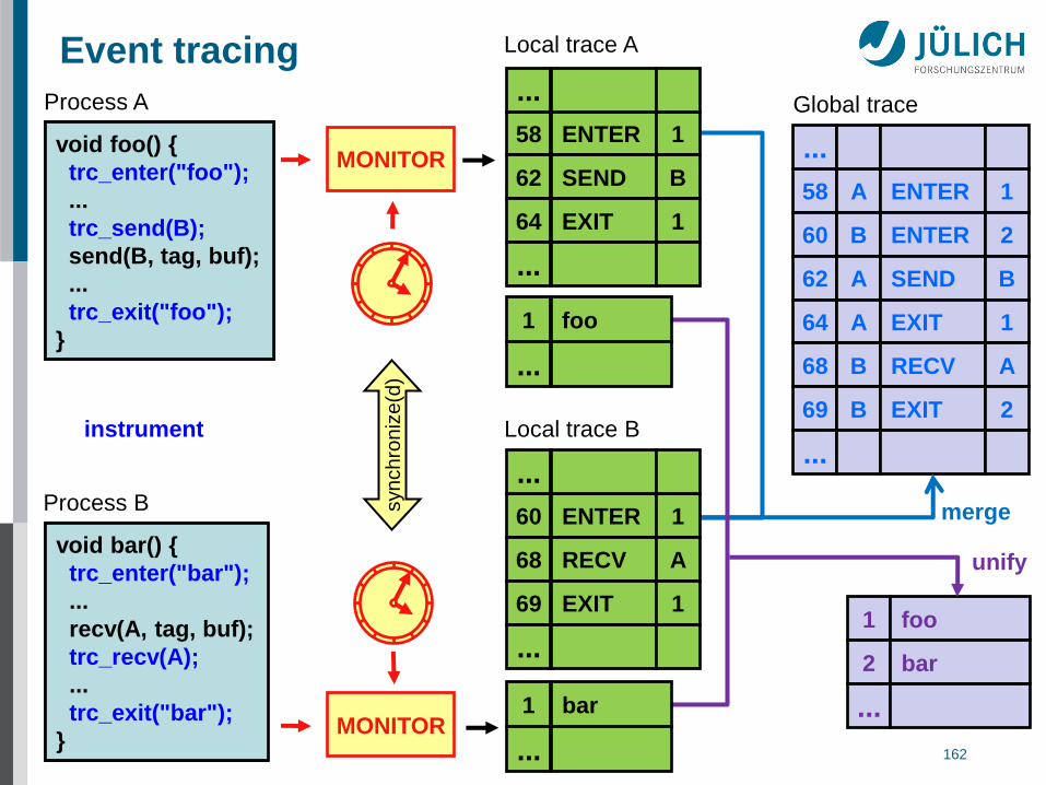
Event tracing
void foo() {
...
send(B, tag, buf);
...
}
Process A
void bar() {
...
recv(A, tag, buf);
...
}
Process B
MONITOR
MONITOR
syn
ch
ron
ize
(d)
void bar() {
trc_enter("bar");
...
recv(A, tag, buf);
trc_recv(A);
...
trc_exit("bar");
}
void foo() {
trc_enter("foo");
...
trc_send(B);
send(B, tag, buf);
...
trc_exit("foo");
}
instrument
Global trace
58 A ENTER 1
60 B ENTER 2
62 A SEND B
64 A EXIT 1
68 B RECV A
...
69 B EXIT 2
...
merge
unify
1 foo
2 bar
...
58 ENTER 1
62 SEND B
64 EXIT 1
...
...
Local trace A
Local trace B
foo 1
...
bar 1
...
60 ENTER 1
68 RECV A
69 EXIT 1
...
...

2013 JSC 163
PMPI: The MPI Profiling Interface
• PMPI allows selective replacement of MPI routines at link time
no re-compilation necessary
• Uses technique of “wrapper” function libraries
• Used by most MPI performance tools
User program
Call MPI_Bcast
Call MPI_Send
MPI Library
MPI_Bcast
PMPI_Send
MPI_Send
MPI library
MPI_Bcast
PMPI_Send
MPI_Send
Wrapper library
MPI_Send
2013 JSC 164
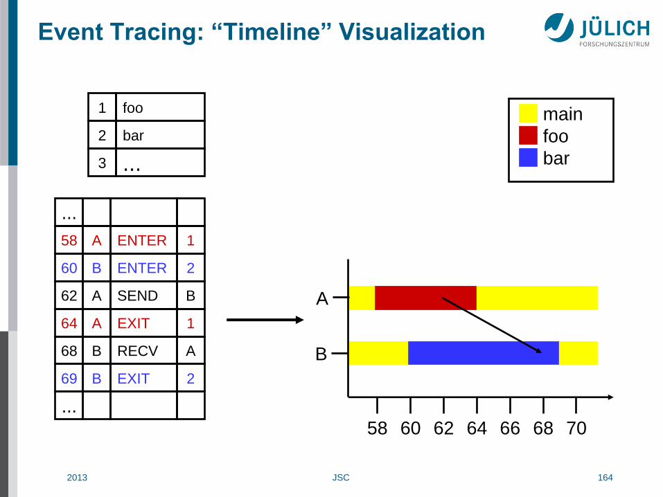
Event Tracing: “Timeline” Visualization
1 foo
2 bar
3 ...
58 A ENTER 1
60 B ENTER 2
62 A SEND B
64 A EXIT 1
68 B RECV A
...
69 B EXIT 2
...
main
foo
bar
58 60 62 64 66 68 70
B
A
2013 JSC 165
Tracing Tools
• MPE / Jumpshot (ANL)
Part of MPICH2
Only supports MPI P2P and collectives; SLOG2 trace format
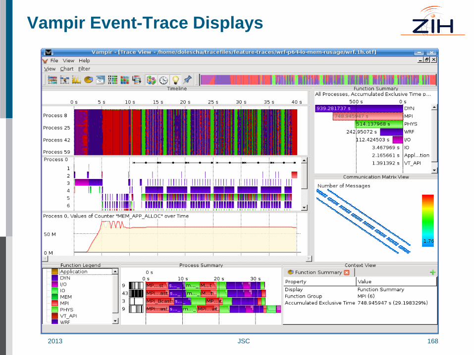
• VampirTrace / Vampir (TU Dresden, ZIH)
http://www.tu-dresden.de/zih/vampirtrace/
http://www.vampir.eu
Open-source measurement system (VampirTrace) + commercial
trace visualizer (Vampir); OTF trace format
• Extrae / Paraver (BSC/UPC)
http://www.bsc.es/paraver
Measurement system (Extrae) and visualizer (Paraver)
Powerful filter and summarization features
Very configurable visualization

2013 JSC 166
Example: Timeline of MPI Ring Program
2013 JSC 167
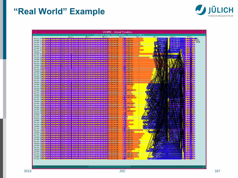
“Real World” Example
2013 JSC 168
Vampir Event-Trace Displays
2013 JSC 169
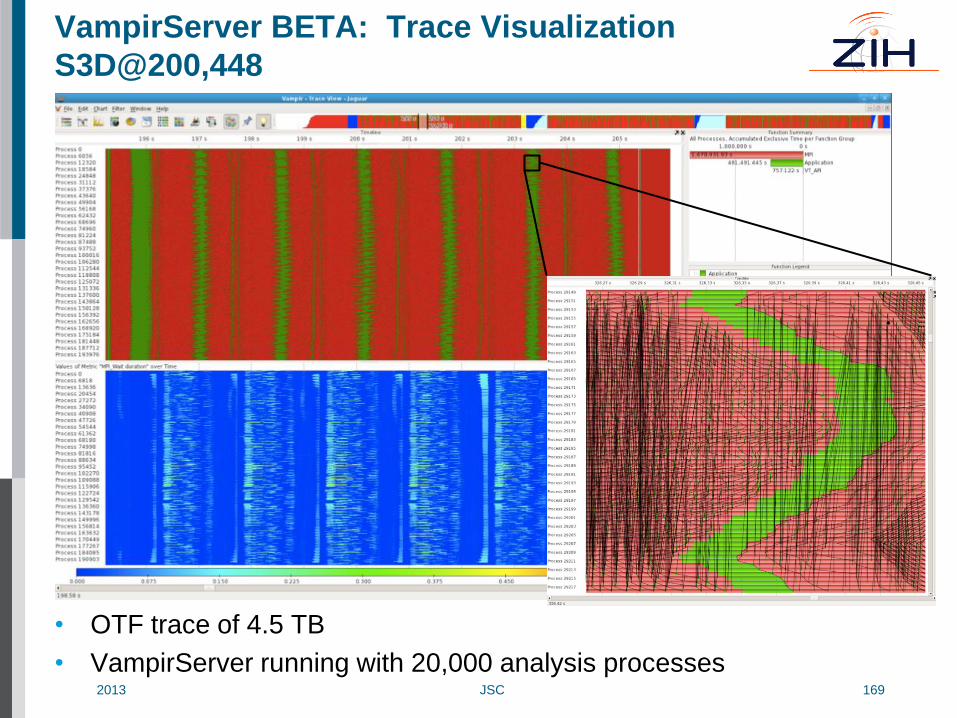
VampirServer BETA: Trace Visualization
S3D@200,448
• OTF trace of 4.5 TB
• VampirServer running with 20,000 analysis processes
2013 JSC 170
Profiling + Tracing Toolsets
• TAU (University of Oregon)
http://tau.uoregon.edu
Very versatile performance analysis toolset for profiling and tracing
Supports many platforms, programming paradigms, and languages
• Scalasca (JSC)
http://www.scalasca.org
Highly scalable call-path profiling
Automatic trace-based performance analysis
Detection, classification and ranking of common parallel
programming bottlenecks
Supports many platforms, programming paradigms, and languages

2013 JSC 171
TAU Profiling, Large System
2013 JSC 172
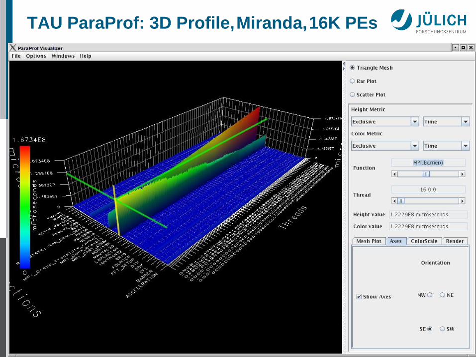
TAU ParaProf: 3D Profile, Miranda, 16K PEs

2013 JSC 173
Scalasca Analysis sweep3D(294,912 Cores)
Measured
metrics
System structure
or topology
Region
tree
2013 JSC 174
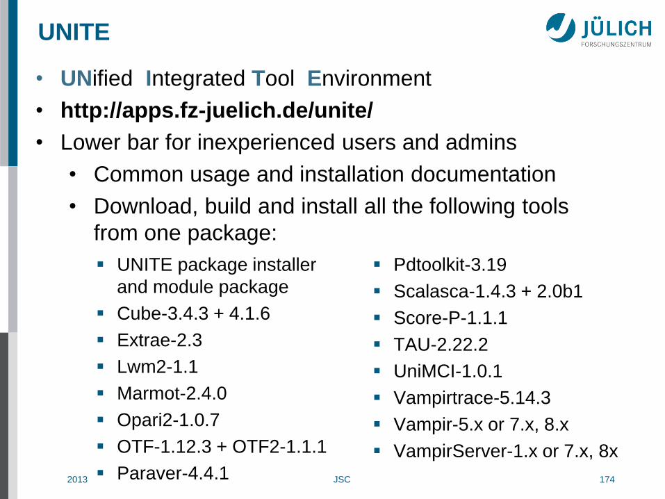
• UNified Integrated Tool Environment
• http://apps.fz-juelich.de/unite/
• Lower bar for inexperienced users and admins
• Common usage and installation documentation
• Download, build and install all the following tools
from one package:
UNITE
UNITE package installer
and module package
Cube-3.4.3 + 4.1.6
Extrae-2.3
Lwm2-1.1
Marmot-2.4.0
Opari2-1.0.7
OTF-1.12.3 + OTF2-1.1.1
Paraver-4.4.1
Pdtoolkit-3.19
Scalasca-1.4.3 + 2.0b1
Score-P-1.1.1
TAU-2.22.2
UniMCI-1.0.1
Vampirtrace-5.14.3
Vampir-5.x or 7.x, 8.x
VampirServer-1.x or 7.x, 8x

2013 JSC 175
Debugging of Parallel Programs
• … is much more difficult than sequential debugging!
• Reasons
Multiplication of sequential bugs on multiple processes
Amount of resources to control and data to handle
Additional kind of bugs in parallel programs, e.g., deadlocks
Non-deterministic behavior non reproducible behavior
Race conditions
Heisenbugs: bugs appear/disappear under debugging
• Commercial parallel debuggers (supporting MPI, threads, CUDA, …)
DDT (Allinea, UK)
http://www.allinea.com
Totalview (TotalView Technologies, Rogue Wave, USA)
http://totalviewtech.com

2013 JSC 176
FUTURE ISSUES FOR HPC
2013 JSC 177
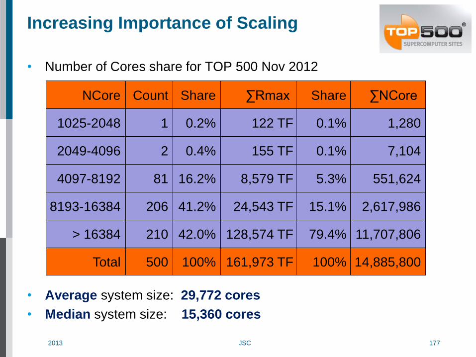
Increasing Importance of Scaling
• Number of Cores share for TOP 500 Nov 2012
• Average system size: 29,772 cores
• Median system size: 15,360 cores
1025-2048
2049-4096
4097-8192
8193-16384
> 16384
NCore
1
2
81
206
210
Count
0.2%
0.4%
16.2%
41.2%
42.0%
Share
122 TF
155 TF
8,579 TF
24,543 TF
128,574 TF
∑Rmax
Total 500 100% 161,973 TF
0.1%
0.1%
5.3%
15.1%
79.4%
Share
100%
1,280
7,104
551,624
2,617,986
11,707,806
∑NCore
14,885,800
2013 JSC 178
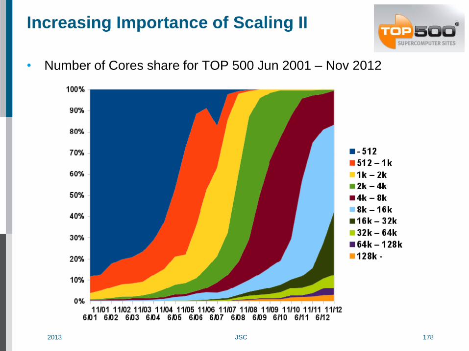
Increasing Importance of Scaling II
• Number of Cores share for TOP 500 Jun 2001 – Nov 2012

2013 JSC 179
Observations
• Petascale is not terascale scaled up!
More than linear increase of scale
Multi-core processors
Multi-mode parallelism
Reduced memory per core
Heterogeneity via HW acceleration (Cell, FPGA, GPU, …)
New programming models (needed)
Higher system diversity
• More emphasis on
Fault-tolerance and performability
Automated diagnosis and remediation
From workshop report
SDTPC Aug 2007
http://www.csm.ornl.gov/workshops/Petascale07/
2013 JSC 180
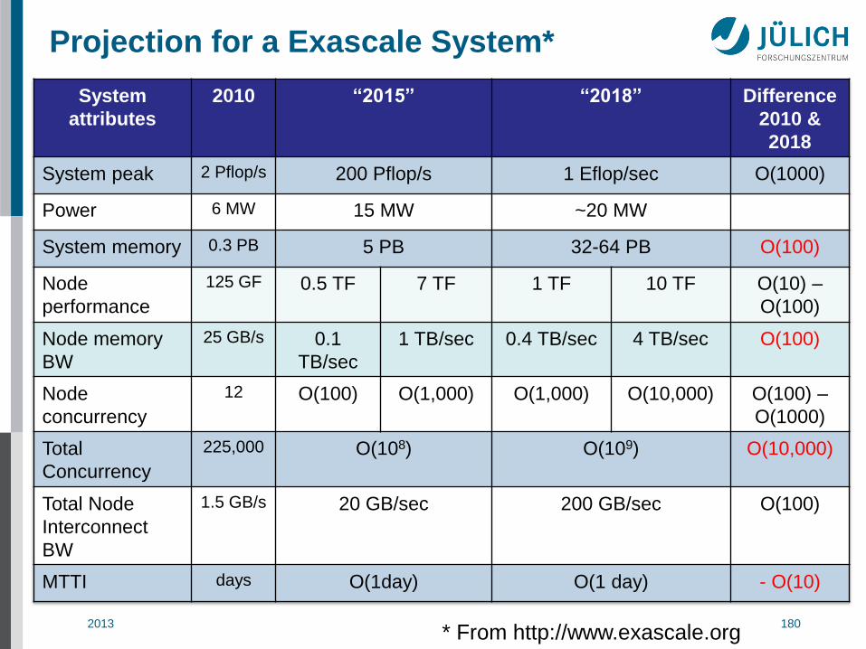
Projection for a Exascale System*
* From http://www.exascale.org
System
attributes
2010 “2015” “2018” Difference
2010 &
2018
System peak 2 Pflop/s 200 Pflop/s 1 Eflop/sec O(1000)
Power 6 MW 15 MW ~20 MW
System memory 0.3 PB 5 PB 32-64 PB O(100)
Node
performance
125 GF 0.5 TF 7 TF 1 TF 10 TF O(10) –
O(100)
Node memory
BW
25 GB/s 0.1
TB/sec
1 TB/sec 0.4 TB/sec 4 TB/sec O(100)
Node
concurrency
12 O(100) O(1,000) O(1,000) O(10,000) O(100) –
O(1000)
Total
Concurrency
225,000 O(108) O(109) O(10,000)
Total Node
Interconnect
BW
1.5 GB/s 20 GB/sec 200 GB/sec O(100)
MTTI days O(1day) O(1 day) - O(10)

2013 JSC 181
IESP
• International Exascale Software Project
• International collaboration
Started Apr 2009
• http://www.exascale.org/
• Objectives
Develop international exascale (system) software roadmap
Investigate opportunities for international collaborations and
funding
Explore governance structure and models for IESP
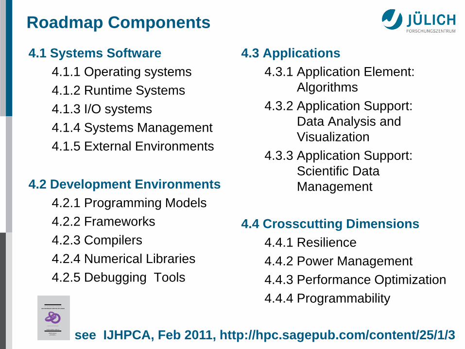
2013 JSC 182
Roadmap Components
4.1 Systems Software
4.1.1 Operating systems
4.1.2 Runtime Systems
4.1.3 I/O systems
4.1.4 Systems Management
4.1.5 External Environments
4.2 Development Environments
4.2.1 Programming Models
4.2.2 Frameworks
4.2.3 Compilers
4.2.4 Numerical Libraries
4.2.5 Debugging Tools
4.3 Applications
4.3.1 Application Element:
Algorithms
4.3.2 Application Support:
Data Analysis and
Visualization
4.3.3 Application Support:
Scientific Data
Management
4.4 Crosscutting Dimensions
4.4.1 Resilience
4.4.2 Power Management
4.4.3 Performance Optimization
4.4.4 Programmability
see IJHPCA, Feb 2011, http://hpc.sagepub.com/content/25/1/3

2013 JSC 183
EESI
• European Exascale Software Initiative
• EU FP7
Funded Jun 2010 to Nov 2011
• http://www.eesi-project.eu/
• Objectives
Develop European exascale system and application software
vision and roadmap
Investigate Europe's strengths and weaknesses
Identify sources of competitiveness for Europe
Investigate and propose programs in education and training for the
next generation of computational scientists
EESI2 started September 2012

2013 JSC 184
We need integrated teams / simulation labs / end stations / ..
To get integrated, customized tool support
Tool community needs to build up interoperable, reusable tool
components implementing the various basic technologies
• We can do performance analysis on the tera- and petascale, however…
Conclusion
Parallel Computing (PC?)
might have reached the masses …
but remember, we do
High Performance Computing (HPC!)