introduction to partial differential equationsfdalio/lecturenotespdefs17.pdf · 2017-09-22 ·...
TRANSCRIPT

INTRODUCTION TO
PARTIAL DIFFERENTIAL EQUATIONS
FS 2017
Prof. Francesca Da Lio
Department of MathematicsETH Zurich
Abstract
These notes are based on the course Introduction to Partial Differential Equations thatthe author held during the Spring Semester 2017 for bachelor and master students inmathematics and physics at ETH.
Contents
1 Generalities on PDEs 21.1 Notation . . . . . . . . . . . . . . . . . . . . . . . . . . . . . . . . . . . . . 2
1.1.1 Multi-indices and derivatives . . . . . . . . . . . . . . . . . . . . . . 31.2 What is a PDE? . . . . . . . . . . . . . . . . . . . . . . . . . . . . . . . . 4
1.2.1 Examples of PDEs . . . . . . . . . . . . . . . . . . . . . . . . . . . 51.2.2 Classification of second order semilinear PDEs . . . . . . . . . . . . 71.2.3 Well-posed problems . . . . . . . . . . . . . . . . . . . . . . . . . . 7
2 First-order PDEs 92.1 The Cauchy Problem . . . . . . . . . . . . . . . . . . . . . . . . . . . . . . 10
2.1.1 Linear equations with constant coefficients . . . . . . . . . . . . . . 102.2 The Method of the Characteristics . . . . . . . . . . . . . . . . . . . . . . 12
2.2.1 A brief description . . . . . . . . . . . . . . . . . . . . . . . . . . . 122.2.2 Applications to quasilinear first order PDEs . . . . . . . . . . . . . 122.2.3 Existence and Uniqueness for the Cauchy Problem . . . . . . . . . 14
2.3 Derivation of characteristic ODEs in the general case . . . . . . . . . . . . 172.3.1 Examples . . . . . . . . . . . . . . . . . . . . . . . . . . . . . . . . 19
2.4 Local Existence: the General case . . . . . . . . . . . . . . . . . . . . . . . 232.4.1 Applications . . . . . . . . . . . . . . . . . . . . . . . . . . . . . . . 26
2.5 Introduction to Hamilton Jacobi Equation . . . . . . . . . . . . . . . . . . 302.5.1 Legendre transform, Hopf-Lax formula . . . . . . . . . . . . . . . . 31
3 Laplace Equation 373.1 Basic Properties . . . . . . . . . . . . . . . . . . . . . . . . . . . . . . . . 373.2 Fundamental solution . . . . . . . . . . . . . . . . . . . . . . . . . . . . . . 40
3.2.1 The Poisson Equation in IRn . . . . . . . . . . . . . . . . . . . . . . 413.3 Sub- and super-harmonic functions . . . . . . . . . . . . . . . . . . . . . . 433.4 Mean-value formulas . . . . . . . . . . . . . . . . . . . . . . . . . . . . . . 46
3.4.1 Properties of harmonic functions . . . . . . . . . . . . . . . . . . . 483.5 Green’s Functions . . . . . . . . . . . . . . . . . . . . . . . . . . . . . . . 57
3.5.1 Derivation of the Green’s Function . . . . . . . . . . . . . . . . . . 58
i

3.5.2 Green’s function for a ball . . . . . . . . . . . . . . . . . . . . . . . 603.5.3 Green’s function for a half space . . . . . . . . . . . . . . . . . . . . 63
3.6 Perron’s Method . . . . . . . . . . . . . . . . . . . . . . . . . . . . . . . . 643.7 Poisson Equations: Classical solutions . . . . . . . . . . . . . . . . . . . . . 693.8 Energy Methods . . . . . . . . . . . . . . . . . . . . . . . . . . . . . . . . . 74
4 Heat equation 774.1 Motivations . . . . . . . . . . . . . . . . . . . . . . . . . . . . . . . . . . . 774.2 Derivation of the Fundamental solution . . . . . . . . . . . . . . . . . . . . 784.3 Homogenous Cauchy Problem . . . . . . . . . . . . . . . . . . . . . . . . . 80
4.3.1 Tychonov’s counterexample . . . . . . . . . . . . . . . . . . . . . . 834.4 Nonhomogeneous Cauchy Problem . . . . . . . . . . . . . . . . . . . . . . 844.5 Maximum Principle . . . . . . . . . . . . . . . . . . . . . . . . . . . . . . . 87
4.5.1 Uniqueness of bounded solutions . . . . . . . . . . . . . . . . . . . 884.6 Mean-value formula . . . . . . . . . . . . . . . . . . . . . . . . . . . . . . . 90
4.6.1 Strong Maximum Principle for the Heat Equation . . . . . . . . . . 934.6.2 Regularity . . . . . . . . . . . . . . . . . . . . . . . . . . . . . . . . 94
4.7 Energy Methods . . . . . . . . . . . . . . . . . . . . . . . . . . . . . . . . . 94
1

Chapter 1
Generalities on PDEs
This Chapter surveys the principal theoretical issues concerning the solving of partialdifferential equations. In Section 1.1 we first list several notations we will use throughoutthese notes. Then we introduce the concept of partial differential equation. In Section1.2 we discuss briefly well-posed problems for partial differential equations.
1.1 Notation
IR denotes the real numbers, C the complex numbers. We will working in IRn and nwill always denote the dimension. Point in IRn will generally be denoted by x, y, ξ, η, thecoordinates of x are (x1, . . . , xn). Occasionally x1, x2, . . . will denote a sequence of pointsin IRn rather than coordinates, but this will always be clear from the context.
If Ω is a subset of IRn, Ω will denote its closure and ∂Ω its boundary.If x, y ∈ IRn we set
x · y =n∑
i=1
xiyi,
so the Euclidean norm of x is given by
|x| = (x · x)1/2.
We use the following notation for sphere and (open) balls in IRn with radius r > 0 andcenter at x:
S(x, r) = ∂B(x, r) = y : |y − x| = r,B(x, r) = y : |y − x| < r
The volume of B(x, r) and the area of S(x, r) are given by
|B(x, r)| = ωn
nrn, and |S(x, r)| = ωnr
n−1
2

where
ωn = |S(x, 1)| = nπn/2
Γ(12n + 1)
Γ(s) =∫∞0ts−1e−tdt is the Euler gamma function. We also denote
−∫
B(x,r)
fdy = average of f over the ball B(x, r)
and
−∫
∂B(x,r)
fdσ(y) = average of f over the sphere ∂B(x, r).
1.1.1 Multi-indices and derivatives
i) A multiindex is vector of the form α = (α1, . . . , αn) where each component αi is anonnegative integer. The order of α is the number |α| = α1 + . . .+ αn .
For x ∈ IRn we setxα = xα1
1 xα22 · · ·xαn
n .
ii) Given a multiindex α and given u : Ω ⊂ IRn → IR define
Dαu(x) :=∂|α|u(x)
∂α1x1 · · ·∂αnxn.
iii) If k is nonnegative integer,
Dku(x) := Dαu(x) : |α| = k .
Special cases
If k = 0, D0u = u.
If k = 1, we regard the elements of Du as being arranged in a vector:
Du = ∇u = (ux1, · · · , uxn) = gradient vector .
If k = 2 we regard the elements of D2u as being arranged in a matrix:
D2u =
ux1x1 · · · ux1xn
.... . .
...uxnx1 · · · uxnxn
= Hessian matrix
v)
∆u =
n∑
i=1
uxixi= tr(D2u) = Laplacian of u.
3
vi) We write the divergence of a vector field F = (F 1, . . . F n) as div(F ) =∑n
i=1 Fixi.
We observe that ∆u = div (Du).
iv) We sometimes employ a subscript attached to the symbols D,D2 etc. to denote thevariables being differentiated . For example if u = u(x, y), x ∈ IRn, y ∈ IRm thenDxu = (ux1, · · · , uxn) and Dyu = (uy1, · · · , uym) .
1.2 What is a PDE?
Partial differential equations are central objects in the mathematical modeling of natu-ral and social sciences (sound propagation, heat diffusion, thermodynamics, electromag-netism, elasticity, fluid dynamics, quantum mechanics, population growth, finance...etc).They were for a long time restricted only to the study of natural phenomena or questionspertaining to geometry, before becoming over the course of time, and especially in thelast century, a field in itself.
A partial differential equation (PDE) is an equation involving an unknown functionof two or more variables and certain of its partial derivatives.
We fix an integer k ≥ 1 and let Ω ⊆ IRn denote an open set .
Definition 1.2.1 An expression of the form
F (x, u(x), Du(x), . . . , Dku(x)) = 0, in Ω (1.1)
is called a kth-order partial differential equation, where
F : Ω× IR× IRn × · · · × IRnk → IR
is given and u : Ω → IR is the unknown.
We solve the PDE if we find all u verifying (1.1) possibly only among those functionssatisfying certain auxiliary boundary conditions on some part Γ of ∂Ω . By finding thesolutions we mean, ideally, obtaining simple, explicit solutions, or, failing that, deducingthe existence and other properties of solutions.
4
Definition 1.2.2 (Classification of PDE) (i) The PDE (1.1) is called lin-ear if it has the form ∑
|α|≤k
aα(x)Dαu(x) = f(x)
for given functions aα. This linear PDE is homogeneous if f ≡ 0 .(ii) The PDE (1.1) is called semilinear if it has the form
∑
|α|=k
aα(x)Dαu(x) + a0(x, u(x), . . . , D
k−1u(x)) = 0
(iii) The PDE (1.1) is called quasilinear if it has the form
∑
|α|=k
aα(x, u(x), . . . , Dk−1u(x))Dαu(x) + a0(x, u(x), . . . , D
k−1u(x)) = 0
(iv) The PDE (1.1) is called fully nonlinear if it depends nonlinearly uponthe highest order derivatives.
1.2.1 Examples of PDEs
There is no general theory known concerning the solvability of all partial differentialequations. Such a theory is extremely unlikely to exist, given the rich variety of physical,geometry, and probabilistic phenomena which can be modeled by PDE.
Following is a list of some specific partial differential equations of interest in currentresearch. We will later discuss the origin and interpretation of these PDE.
Throughout x ∈ Ω where Ω ⊆ IRn is an open set, and t ≥ 0. Also Du = Dxu denotesthe gradient of u with respect to the spatial variable x and the variable t always denotestime.
1. Linear Transport Equation:
ut + b(x, t) ·Du(x, t) = 0, (x, t) ∈ Ω ⊂ IRn × (0,+∞) ,
it is a linear first order equation.
2. Laplace equation:
∆u(x) =n∑
i=1
uxixi= 0, x ∈ Ω ⊂ IRn
it is a linear second order equation.
5

3. Heat or diffusion equation:
ut(x, t)− k∆u(x, t) = 0 (x, t) ∈ Ω ⊂ IRn × (0,+∞) .
it is a linear second order equation.
4. Wave equation:
utt(x, t)− c2∆u(x, t) = 0 (x, t) ∈ Ω ⊂ IRn × (0,+∞) .
it is a linear second order equation.
5. Poisson equation:∆u(x) = f(x), x ∈ Ω ⊂ IRn
it is a linear second order equation.
6. Nonlinear Poisson equation:
∆u(x) = f(u), x ∈ Ω ⊂ IRn
it is a semilinear second order equation.
7. Minimal surface equation
div
(Du
(1 + |Du|2)1/2)
= 0
it is a quasilinear second order equation.
8. Schrodinger’s equationiut +∆u = 0.
it is a linear second order equation.
9. Monge-Ampere equation
Det(D2u) = f(x) x ∈ Ω ⊂ IRn.
it is a fully nonlinear second order equation.
10. Hamilton-Jacobi equation
H(x, u,Du) = 0 x ∈ Ω ⊂ IRn
orut +H(x, u,Du) = 0 (x, t) ∈ Ω ⊂ IRn × (0,+∞) ,
they are fully nonlinear first order equations.
11. Scalar conservation law
ut + div(F (u)) = 0 (x, t) ∈ Ω ⊂ IRn × (0,+∞) ,
the vector field F (u) depends nonlinearly upon u.
6
1.2.2 Classification of second order semilinear PDEs
The second order semilinear PDEs can be classified in elliptic, parabolic and hyper-bolic. To describe such a classification it is convenient to consider the time as a spacecoordinate, by setting xn+1 = t. Set N = n + 1, the unknown function is written asu = u(x1, . . . , xN ) and the equation (1.1) can be written in the form
N∑
i,j=1
Aij(x)uxixj+ A0 = 0 (1.2)
where Aij are the coefficients of a N × N symmetric matrix and A0 is a function thatmay depend on u and its first derivatives. The quadratic term
∑ni,j=1Aij(x)uxixj
is calledprincipal part of the differential equation.
The equation (1.2) is called elliptic if the signature(1) of the matrix Aij is (N, 0) or(0, N) (namely the matrix is positive definite or negative definite). The (1.2) is calledparabolic if the signature of the matrix Aij is (N − 1, 0) or (0, N − 1) and it is calledhyperbolic if the signature of the matrix Aij is (N − 1, 1) or (1, N − 1). We notice thatthe Laplace equation is elliptic, the diffusion equation is parabolic and the wave equationis hyperbolic.
1.2.3 Well-posed problems
What is the meaning of solving partial differential equations? Ideally, we obtain explicitsolutions in terms of elementary functions. In practice this is only possible for verysimple PDEs, and in general it is impossible to find explicit expressions of all solutions ofall PDEs. In the absence of explicit solutions, we need to seek methods to prove existenceof solutions of PDEs and discuss properties of these solutions.
Hadamard introduced the notion of well-posed problems. A given problem for a partialdifferential equation is well-posed if
(i) there is a solution;
(ii) this solution is unique;
(iii) the solution depends continuously in some suitable sense on the data given in theproblem, i.e., the solution changes by a small amount if the data change by a smallamount.
Clearly it would be desirable to “solve” a PDE in such a way that (i)-(iii) hold. Noticethat we have not specified what we mean by a “solution”. Should we ask, for example thata “solution” u must be real analytic or at least infinitely differentiable? This might be
(1)Recall: the signature of Aij is the pair (p, q) where p is the number of positive eigenvalues and q isthe number of negative eigenvalues
7

desirable, but perhaps we are asking too much. It would be wiser to require a solution ofa PDE of order k to be at least k times continuously differentiable. Let us informally calla solution with such smoothness a classical solution. So by solving a partial differentialequation in the classical sense we mean if possible to write down a formula for a classicalsolution satisfying (i)− (iii) above.
Unfortunately most PDEs cannot be solved in a classical sense and we are forced toabandon the search for smooth classical solutions. We must instead investigate a widerclass of candidates for solutions. If from the beginning we demand that our solutions bevery regular, then we are usually going to have a really hard time finding them, as ourproofs must then necessarily include possibly intricate demonstrations that the functionswe are building are in fact smooth enough. A more reasonable strategy is to consideras separate the existence and the regularity problems. The idea is to define for a givenPDE a reasonable notion of a weak solution, with the expectation it may be easier toestablish its existence, uniqueness and continuous dependence on the data. For variouspartial differential equations this is the best that can be done. For other equations we canhope that our weak solution may turn out after all to be smooth to qualify as a classicalsolution. This leads to the question of regularity of weak solutions which usually restsupon many intricate calculus estimates.
Example 1.2.1 (Counterexample of Hadamard) Consider the problem of finding aharmonic function in E taking either Dirichlet data or Neumann data on a portion Σ1 of∂E and Dirichlet data on the remaining part Σ2 = ∂E \ Σ1. Such a problem is ill-posed.Even if a solution exits, in general it is not stable in any reasonable topology, as shownby the following example due to Hadamard. The boundary value problem
uxx + uyy = 0 in (−π/2, π/2)× (0,+∞)u(±π/2, y) = 0 y > 0u(x, 0) = 0 x ∈ (−π/2, π/2)
uy(x, 0) = e−√n cos(nx) x ∈ (−π/2, π/2)
admits the family of solutions
un(x, y) = e−√n 1
ncos(nx) sinh(ny), n odd integer.
One verifis that‖un,y(x, 0)‖L∞(−π/2,π/2) → 0 as n→ +∞
and for y > 0‖un(·, y)‖L∞(−π/2,π/2) → +∞, as n→ +∞.
8
Chapter 2
First-order PDEs
In this chapter we search for explicit formulas for general first-order nonlinear partialdifferential equations of the form
F (x, u,Du) = 0 in Ω (2.1)
subject to the boundary condition
u = g on Γ ⊂ ∂Ω (2.2)
where Ω ⊂ IRn is open. Here F : Ω × IR × Rn → IR, g : Γ → IR are given and they aresupposed smooth functions, u : Ω → IR is the unknown.
We introduce the basic notion of noncharacteristic hypersurfaces for initial-value prob-lems. We solve initial-value problems by the method of characteristics if the initial valuesare prescribed on noncharacteristic hypersurfaces.
We also introduce the Hopf-Lax formula for Hamilton-Jacobi equations and study itsregularity properties.
Notation. Let us write F = F (x, z, p), for p ∈ IRn, z ∈ IR, x ∈ Ω . Thus p isthe name of the variable for which we substitute the gradient Du(x) and z isthe variable for which we substitute u(x). We also assume hereafter that F issmooth and set
DpF = (Fp1, . . . Fpn)DzF = Fz
DxF = (Fx1, . . . Fxn) .(2.3)
9
2.1 The Cauchy Problem
The problem (2.1)-(2.2) is called the Cauchy Problem associated to the equation (2.1). Aparticular case is a problem of the form
ut +G(x, t, u,Dxu) = 0 in Ω = U × [0,+∞)
u(x, 0) = g(x) for x ∈ U(2.4)
where U ⊂ IRn is an open set and G : U × (0,+∞)× IR × IRn → IR and g : U → IR aregiven functions. In this case the independent variables are (x, t), where x = (x1, . . . , xn)is the spatial variable, and t is the time variable, Γ = U × 0. The equation in (2.4) isassociated to an operator F = ∂t+G where G does not depend on ∂t. In this context theboundary condition (2.2) is called initial condition.
2.1.1 Linear equations with constant coefficients
Homogeneous caseWe consider the so-called transport equation with constant coefficients:
ut + b ·Du = 0 in IRn × (0,+∞), (2.5)
where b = (b1, . . . , bn) ∈ IRn is a fixed vector and u : IRn × (0,+∞) → IR is the unknownu = u(x, t). Here x = (x1, . . . , xn) ∈ IRn denotes a typical point in space and t ≥ 0denotes the time.
The equation (2.5) describes for instance the transport of a solid polluting substancealong a channel; here u is the concentration of the substance and b is the stream speed.
Which functions u solve (2.5)?
Let us suppose for the moment we are given some smooth solution u and try tocompute it. We observe that given (x, t) for every s ∈ IR we have
0 = ut(x+ sb, t + s) + b ·Du(x+ sb, t+ s) =d
dsu(x+ sb, t + s). (2.6)
Therefore the function z(s) = u(x+sb, t+s) is a constant function of s and consequently foreach point (x, t), u is constant on the line through (x, t) with the direction (b, 1) ∈ IRn+1.Hence if we know the value of u at any point on each such line, we know its valueeverywhere.
Let us consider the initial-value problemut + b ·Du(x, t) = 0 in IRn × [0,+∞)
u(x, 0) = g(x) for x ∈ IRn.(2.7)
10
Here b ∈ IRn and g : IRn → IR are known and the problem is to compute u. Given (x, t),the line through (x, t) with direction (b, 1) is represented parametrically by (x+ sb, t+ s)(s ∈ IR). This line hits the hypersurface Γ := IRn × 0 when s = −t at the point(x− tb, 0). Since u is constant on the line and u(x− tb, 0) = g(x− tb), we deduce
u(x, t) = g(x− tb) (x ∈ IRn, t ≥ 0). (2.8)
So if (2.7) has a sufficiently regular solution u, it must be given by (2.8). And con-versely it is easy to check directly that if g ∈ C1 then u defined by (2.8) is indeed asolution of (2.7).
The formula (2.8) says that the initial data is propagated along the curves x = x0+ btand for this reason the equation (2.5) is known as the transport equation.
Nonhomogeneous problemNext let us look at the associated nonhomogeneous problem
ut + b ·Du(x, t) = f(x, t) in IRn × [0,+∞)
u(x, 0) = g(x) for x ∈ IRn.(2.9)
As before fix (x, t) ∈ Rn+1 and set z(s) = u(x+ sb, t+ s) for s ∈ IR. Then
z(s) = b ·Du(x+ sb, t + s) + ut(x+ sb, t+ s) = f(x+ sb, t+ s).
Consequently
u(x, t)− g(x− bt) = z(0)− z(−t) =∫ 0
−t
z(s)ds
=
∫ 0
−t
f(x+ sb, t+ s)ds
=
∫ t
0
f(x+ (s− t)b, s)ds;
and so
u(x, t) = g(x− tb) +∫ t
0f(x+ (s− t)b, s)ds (2.10)
solves the initial problem (2.9).
Remark 2.1.1 Observe that we have derived our solutions (2.8) and (2.10) byin effect converting the partial differential equations into ordinary differentialequations. This is a special case of the method of characteristics that wedevelop later.
11
2.2 The Method of the Characteristics
2.2.1 A brief description
The method of characteristics was developed in the middle of the nineteenth century byHamilton. It consists in converting the Cauchy problem (2.1)-(2.2) into a Cauchy problemfor an appropriate system of ODEs (the so-called characteristic equations). Thesolutions of the characteristic equations parametrize the so-called characteristic curves,which pass through the following (n− 1)- dimensional manifold
S0 = (x, g(x)), x ∈ Γ (2.11)
which is called initial manifold.Let us denote by Cp the characteristic curve which passes through p ∈ S0. We suppose
that for some p ∈ S0 the curve Cp is not tangent to S0 . Then by continuity the sameholds for all the curves Cp for p in a neighbourhood N of p. The construction of thecharacteristic equations is made in such a way that the set of the characteristics curves Cpwith p in a neighbourhood N of p constitute a n − 1 dimensional surface correspondingto the graph of a solution of the PDE in consideration. Such a solution is constructed ina a neighborhood N of p.
The existence of the characteristic curves and the fact that S0 is a manifold requiresome regularity assumptions on F and g. The construction of the characteristic equationdepend on the structure of the partial differential equation in consideration.We start byexamining this method in the case of quasilinear first order PDEs and we study later thegeneral case of fully nonlinear equations.
2.2.2 Applications to quasilinear first order PDEs
For simplicity we start with the case of quasilinear PDEs of the form
c(x, u) ·Du+ b(x, u) = 0 (2.12)
where x = (x1, x2) ∈ Ω ⊆ IR2, b ∈ C1(Ω× IR) , c ∈ C1(Ω× IR).We are interested in studying classical solutions of (2.12), namely functions u : D → IR
of class C1 that verify c(x, u(x)) ·Du(x)+ b(x, u(x)) = 0 for every x ∈ D ⊆ Ω . The graphof the solution u is given by
S = (x, u(x)) : x ∈ Dwith D = domu. S is called integral surface for the equation (2.12). Solving the equa-tion (2.12) means to find all the integral surfaces. We recall that if S is a 2-dimensionalsurface of IR3 then the normal unit vector to S at the generic point q = (x, u(x)) is givenby
NS(q) =1√
1 + |Du|2(−Du(x), 1) .
12
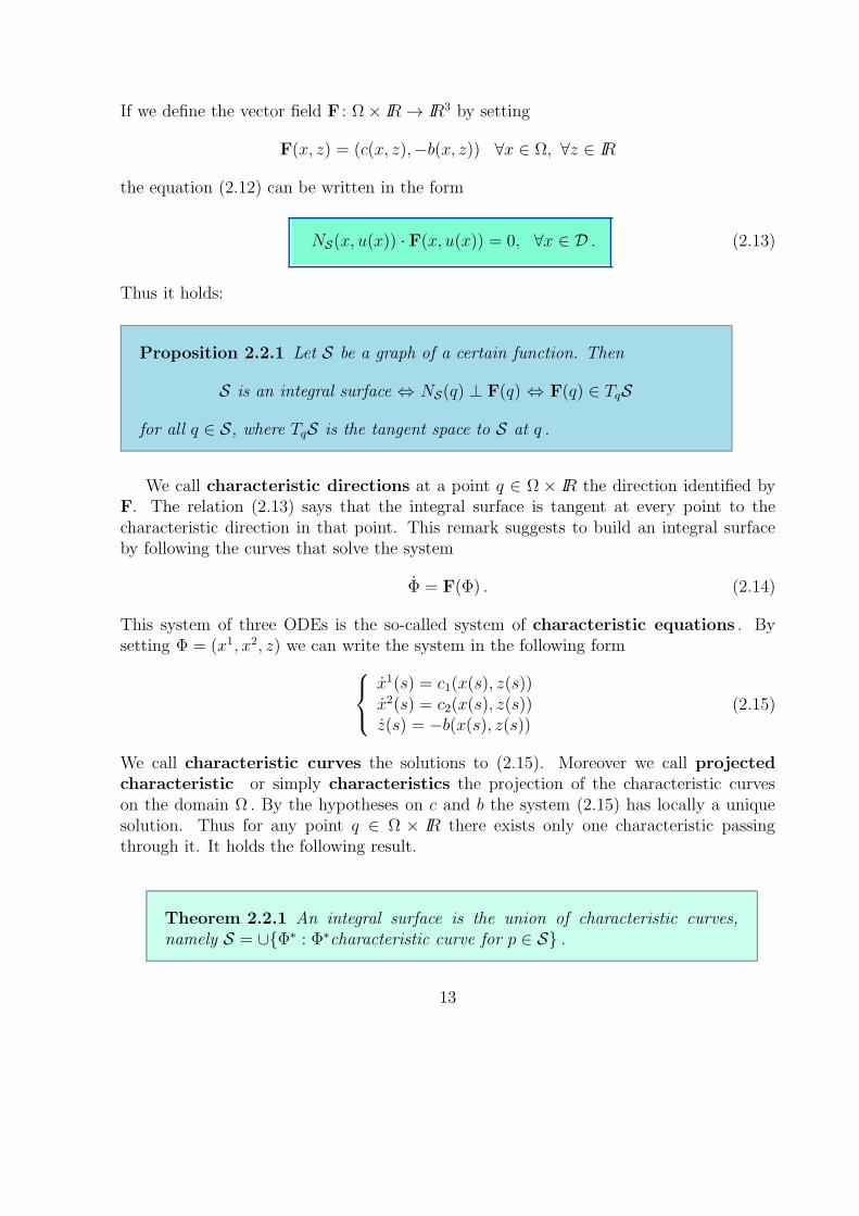
If we define the vector field F : Ω× IR → IR3 by setting
F(x, z) = (c(x, z),−b(x, z)) ∀x ∈ Ω, ∀z ∈ IR
the equation (2.12) can be written in the form
NS(x, u(x)) · F(x, u(x)) = 0, ∀x ∈ D . (2.13)
Thus it holds:
Proposition 2.2.1 Let S be a graph of a certain function. Then
S is an integral surface ⇔ NS(q) ⊥ F(q) ⇔ F(q) ∈ TqS
for all q ∈ S, where TqS is the tangent space to S at q .
We call characteristic directions at a point q ∈ Ω × IR the direction identified byF. The relation (2.13) says that the integral surface is tangent at every point to thecharacteristic direction in that point. This remark suggests to build an integral surfaceby following the curves that solve the system
Φ = F(Φ) . (2.14)
This system of three ODEs is the so-called system of characteristic equations . Bysetting Φ = (x1, x2, z) we can write the system in the following form
x1(s) = c1(x(s), z(s))x2(s) = c2(x(s), z(s))z(s) = −b(x(s), z(s))
(2.15)
We call characteristic curves the solutions to (2.15). Moreover we call projectedcharacteristic or simply characteristics the projection of the characteristic curveson the domain Ω . By the hypotheses on c and b the system (2.15) has locally a uniquesolution. Thus for any point q ∈ Ω × IR there exists only one characteristic passingthrough it. It holds the following result.
Theorem 2.2.1 An integral surface is the union of characteristic curves,namely S = ∪Φ∗ : Φ∗characteristic curve for p ∈ S .
13

Proof of Theorem 2.2.1. Let S be an integral surface namely S is the graph ofu : D → IR solution of (2.12). Fix a point q = (x, u(x)) ∈ S and consider the solution(x(·), z(·)) of (2.15) such that x(0) = x and z(0) = u(x). This solution will be definedin a certain open interval I containing the origin and such that x(s) ∈ Ω for all s ∈ I .It is enough to show that the parametrized curve is completely contained in S. To thispurpose we consider the function
ϕ(s) = z(s)− u(x(s)) ∀s ∈ I.
We have
ϕ(s) = z(s)−Du(x(s)) · x(s)= −b(x(s), z(s)) −Du(x(s)) · c(x(s), z(s))= −b(x(s), ϕ(s) + u(x(s)))−Du(x(s)) · c(x(s), ϕ(s) + u(x(s))) .
Thus ϕ is a solution of the Cauchy problem
ϕ = f(s, ϕ)ϕ(0) = 0 ,
where f is defined in a neighborhood of (0, 0) in IR2 by:
f(s, y) = −b(x(s), y + u(x(s)))−Du(x(s)) · c(x(s), y + u(x(s))) .
The function f is continuous in I×IR and it is locally Lipschitz continuous with respect toy. This guarantees the uniqueness of the solution. It follows that ϕ(s) ≡ 0 for every s ∈ I(the function identically zero is a solution of the Cauchy problem). Thus (x(s), z(s)) ∈ Sfor every s ∈ I and this concludes the proof. 2
Philosophically speaking, one might say that the characteristic curves take with theman initial piece of information of the initial integral surface, and propagate it with them.
Corollary 2.2.1 If two integral surfaces intersect at a point, then they inter-sect along the characteristic curve that passes through that point.
2.2.3 Existence and Uniqueness for the Cauchy Problem
We consider now the Cauchy problem
c(x, u) ·Du+ b(x, u) = 0 in Ωu = g on Γ
(2.16)
14

where Γ ⊂ ∂Ω is a regular curve contained in Ω and g : Γ → IR is a given function, whichis of class C1 is a neighborhood of Γ.
We are interested in finding local solutions to (2.16) in a neighborhood of x ∈ Γ,namely classical solutions of the equation (2.12) defined in an open neighborhood D of xand such that u(x) = g(x), for x ∈ D ∩ Γ . We show the following result:
Theorem 2.2.2 Let x ∈ Γ be such that
c(x, g(x)) /∈ TxΓ , (2.17)
then the problem (2.16) has a unique local solution in a neighborhood of x .
The hypothesis (2.17) is called transversality condition and it says that the pro-jected characteristic through x is not tangent to Γ. In this case we also say thatthe curve Γ is noncharacteristic for the Cauchy Problem (2.16) at the point x.
Proof of Theorem 2.2.2. Let ϕ : I ⊆ IR → IR2, r 7→ (ϕ1(r), ϕ2(r)) be a regular(ϕ′(r) 6= 0) C1 parametrization of Γ, such that ϕ(r) = x . We define h(r) = g(ϕ(r)) forall r ∈ I. The boundary condition can be written as u(x) = h(r) for all r ∈ I. For everyr ∈ I the Cauchy problem
x1(s) = c1(x(s), z(s))x2(s) = c2(x(s), z(s))z(s) = −b(x(s), z(s))x1(0) = ϕ1(r)x2(0) = ϕ2(r)z(0) = h(r)
(2.18)
admits a unique solution defined in a neighborhood of 0 and it may depend on r. Ifr is in a compact W ⊂ I containing r then the domain of the solution of (2.18) canbe taken independent of r.(1) Let us denote by (X(r, ·), Z(r, ·)) the solution of (2.18)which is defined in an interval J containing 0. From the theory of ODEs it follows that
(1)In the qualitative theory of ODEs the following result holds: Given an open interval I ⊂ IR and anopen set D ⊂ IRn and f : I ×D → IRn continuous and locally Lipschtiz continuous with respect to thesecond variable, then for every K ⊂ I ×D compact, there is δ > 0 such that for every (x0, t0) ∈ K theCauchy problem u(t) = f(t, u), u(t0) = x0 admits a unique solution in (t0 − δ, t0 + δ).
15

X : W × J → IR2, and Z : W × J → IR are C1(W × J)(2) and satisfy
Xs(r, s) = c(X(r, s), Z(r, s))Zs(r, s) = −b(X(r, s), Z(r, s))X(r, 0) = ϕ(r)Z(r, 0) = h(r).
(2.19)
Claim 1: There is an open neighborhood W ⊆ W of r and an open interval J ⊆J containing 0, such that the function (r, s) 7→ X(r, s) is invertible from W × J intoX(W × J) =: D . Its inverse function is C1
Proof of the Claim 1. We verify that X satisfies the hypotheses of the InverseFunction Theorem(3) in (r, 0) ∈ W × J . We know that X ∈ C1 in an open neighborhoodof (r, 0). Moreover
DX(r, 0) = (Dϕ(r), c(X(r, 0), Z(r, 0)) = (Dϕ(r), c(x, g(x)) .
We observe that the matrix DX(r, 0) is invertible by the transversality condition. Theclaim is thus proved.
Hence there are functions S,R : D → IR of class C1(D) such that
x = X(R(x), S(x)), for all x ∈ D .
We define u : D → IR by setting
u(x) = Z(R(x), S(x)), for all x ∈ D .
.Claim 2: u is a local solution of (2.12).Proof of the Claim 2.We observe that u ∈ C1(D), since it is the composition of functions of class C1. If
x ∈ D ∩ Γ then S(x) = 0 and if we set r = R(x) we have ϕ(r) = X(r, 0) = x andu(x) = g(ϕ(r)) = g(x) . We can represent the graph of u through the maps R and S:
S = (x, u(x) : x ∈ D = (X(r, s), Z(r, s)) : (r, s) ∈ W × J .(2)Differentiable dependence on the data of the solution of the Cauchy Problem: Given an
open interval I ⊂ IR and an open set D ⊂ IRn and f : I ×D → IRn continuous. Suppose that for every(x0, t0) ∈ I×D there exists a unique solution φ(·, t0, x0) of the Cauchy Problem u(t) = f(t, u), u(t0) = x0
which is defined in (t0 − δ, t0 + δ) with δ > 0 independent of (t0, x0). If f is of class C1 in I ×D then themap (t, t0, x0) 7→ φ(·, t0, x0) is of class C
1 in (t0 − δ, t0 + δ)× I ×D.(3)Inverse Function Theorem: Let A ⊂ IRn be an open set and x0 ∈ A and f : A → IRn be of class
C1 such that Df(x0) is invertible (Jacf (x0) 6= 0). Then there exits an open neighborhood A of x0 such
that f : A → f(A) is invertible and the inverse is of class C1.
16
We observe that the tangent space TpS at the point p = (X(r, s), Z(r, s)) is generated bythe vectors ((Xr(r, s), Zr(r, s))) and ((Xs(r, s), Zs(r, s))). Since
F (p) = (c(X(r, s), Z(r, s)),−b(X(r, s), Z(r, s))
we get that F (p) ∈ TpS . Therefore u is a solution of the equation (2.12) .
Claim 3: Uniqueness of the maximal solution.Proof of the Claim 3. We suppose that the solution we have built has a maximal
domain D (namely it cannot be extended in a larger domain). We take another solutionu with dom(u)=D We set
S0 = (x, u(x)) : x ∈ Γ ∩ D, S0 = (x, u(x)) : x ∈ Γ ∩ D .
By the maximality of u we have S0 ⊆ S0. Then by the Corollary 2.2.1 we have S ⊆ S.Thus the maximal solution is unique.
We can conclude the proof of Theorem 2.2.2 2
Remark 2.2.1 We observe that Theorem 2.2.2 does not provide an explicitformula for the solution of the Cauchy Problem but a constructive way to getthe solution that can be adopted in several specific case.
2.3 Derivation of characteristic ODEs in the general
case
We return to the general equation
F (x, u,Du) = 0 in Ω (2.20)
subject to the boundary condition
u = g on Γ ⊂ ∂Ω (2.21)
where Ω ⊂ IRn is open.Also in this case we are going to convert the PDE into an appropriate system of ODEs.
Suppose u solves (2.20)-(2.21) and fix any point x ∈ Ω. We would like to calculate u(x)by finding some curves lying within Ω, connecting x with a point x0 ∈ Γ and along whichwe can compute u at the one end x0. We hope then to be able to calculate u all along thecurve, and so particularly in x.
Finding the characteristic ODEs. Let us suppose the characteristic curve is de-scribed parametrically the function x(s) = (x1(s), . . . xn(s)), the parameter s lying in some
17
subinterval of IR . Assuming u is a C2 solution of (2.20), we define also z(s) := u(x(s))and in addition we set p(s) := Du(x(s)) . So z(s) gives the values of u along the curveand p(s) records the values of the gradient Du . We must choose the function x(·) in sucha way that we can compute z(·) and p(·) .
For this we differentiate p(s) and we get
pi(s) =n∑
j=1
uxixj(x(s))xj(s) . (2.22)
Now we differentiate the PDE (2.20) with respect of xi:
n∑
j=1
Fpj(x, u,Du)uxixj+ Fz(x, u,Du)uxi
+ Fxi(x, u,Du) = 0 . (2.23)
We are able to employ this identity to get rid of the second derivatives terms in (2.22) ifwe set for j = 1, · · · , n
xj(s) = Fpj(x(s), z(s), p(s)) . (2.24)
We evaluate (2.23) at x = x(s) and we obtain the identity
n∑
j=1
Fpj(x(s), z(s), p(s))uxixj+ Fz(x(s), z(s), p(s))p
i(s) (2.25)
+ Fxi(x(s), z(s), p(s)) = 0 .
By combining (2.24), (2.25) and (2.22) we get
pi(s) = −Fz(x(s), z(s), p(s))pi(s)− Fxi
(x(s), z(s), p(s)) . (2.26)
Finally
z(s) =
n∑
j=1
pj(s)Fpj(x(s), z(s), p(s)) . (2.27)
By summarizing we get the following system of 2n+ 1 ODEs:
(a)p(s) = −DzF (x(s), z(s), p(s))p(s)−DxF (x(s), z(s), p(s))(b)z(s) = DpF (x(s), z(s), p(s)) · p(s)(c)x(s) = DpF (x(s), z(s), p(s)).
(2.28)
This system of 2n+1 first-order ODE comprises the characteristic equations of the nonlin-ear PDE (2.20). The functions p(·), z(·), x(·) are called the characteristics. We refer to x(·)as the projected characteristic: it is the projection of the full characteristics (p(·), z(·), x(·))onto the region Ω ⊆ IRn .
We have shown:
18

Theorem 2.3.1 (Structure of characteristic ODEs) Let u ∈ C2(Ω)solve the nonlinear, first-order partial differential equation (2.1). Assume x(·)solve the ODE (2.28)(c), where p(·) = Du(x(·)), z(·) = u(x(·)) . Then p(·)solves the ODE (2.28)(a) and z(·) solves the ODE (2.28)(b), for those s forwhich x(·) ∈ Ω .
Remark 2.3.1 The key step in the derivation is the setting x = DpF sothat the terms involving second derivatives drop out. We obtain closure ofthe system, and in particular we are not forced to introduce ODEs for higherderivatives of u .
2.3.1 Examples
We consider some special cases for which the structure of the characteristic equationsis simple. We show how we can sometimes actually solve the characteristic ODEs andthereby explicitily compute solutions of certain first-order PDEs, subject to appropriateboundary conditions.
a. F linear
F (x, u,Du) = b(x)u(x) + c(x) ·Du = 0.
Then F (x, z, p) = b(x)z + c(x) · p and so
DpF = c(x) .
The equation (2.28)(c) becomesx(s) = c(x(s)) ,
an ODE involving only the function x(·). Furthermore equation (2.28)(b) becomes
z(s) = c(x(s)) · p(s) = −b(x(s))z(s) .
In summary x(s) = c(x(s))z(s) = −b(x(s))z(s) (2.29)
comprise equations for the linear, first-order PDE (the equation for p(·) is not needed).a. F quasilinearThis case has been already considered in the section 2.2.2:
F (x, u,Du) = b(x, u(x)) + c(x, u(x)) ·Du = 0.
19

Then F (x, z, p) = b(x, z) + c(x, z) · p and so
DpF = c(x, z) .
The equation (2.28)(c) becomes
x(s) = c(x(s), z(s)) .
Furthermore equation (2.28)(b) becomes
z(s) = −b(x(s), z(s)) .
Consequently x(s) = c(x(s), z(s))z(s) = −b(x(s), z(s)) (2.30)
are the characteristic equations for the quasilinear first-order PDE (once again the equa-tion for p() is not needed).
Example 2.3.1 We consider the simpler case of a boundary-value problem for a semi-linear PDE:
ux1 + ux2 = u2 in x2 > 0u = g in x2 = 0 (2.31)
In this case c = (1, 1) and b = −z2. Then (2.30) becomes
x1(s) = 1, x2(s) = 1z(s) = z2
(2.32)
Consequently x1(s) = x0 + s, x2(s) = s
z(s) = z0
1−sz0= g(x0)
1−sg(x0)
(2.33)
where x0 ∈ IR, s ≥ 0, provided the dominator is not zero. Fix a point (x1, x2) ∈ x2 > 0so that (x1, x2) = (x1(s), x2(s)) = (x0 + s, s), that is x0 = x1 − x2 and s = x2. Then
u(x1, x2) = u(x1(s), x2(s)) = z(s) =g(x0)
1− sg(x0)
=g(x1 − x2)
1− x2g(x1 − x2).
This solution makes sense only if 1− x2g(x1 − x2) 6= 0.
20

Example 2.3.2 We consider the problem
1)
xux + yuy = x+ yey in Ωu(x, y) = ex on Γ .
where Ω = y 6= x+ 1 and Γ = y = x+ 1 .Solution.i) Parametrization of the boundary condition. The graph of the line y = x+ 1 can be
parametrized by ϕ(r) = (r, r + 1). We set h(r) = u(r, r + 1) .ii) Characteristic equations.
x(s) = x(s)y(s) = y(s)z(s) = x(s) + y(s)ey(s)
(2.34)
The initial conditions for the system (2.34) are
x(0) = ry(0) = r + 1z(0) = er
(2.35)
The general solution is
x(r, s) = res
y(r, s) = (r + 1)es
z(r, s) = res + exp((r + 1)es) + (1− e)er − r.(2.36)
Now we want to invert (r, s) 7→ (x(r, s), y(r, s)).(iii) Invertibility of the function (r, s) 7→ (x(r, s), y(r, s)). We have to solve the system
x = res
y = (r + 1)es(2.37)
The solution is r = r(x, y) := x
y−x
s = s(x, y) := log(y − x)(2.38)
in the half-plane y > x .(iv) Writing of the solution in function of x and y. The solution is
u(x, y) = z(r(x, y), s(x, y))
= x+ ey + (1− e) exp (x
y − x)− x
y − x.
We observe that even if the coefficients of the PDE are C∞(IR2) as the initial condition,the solution may not be defined in all IR2 .
21

Example 2.3.3 (Failure of the transversality condition) The following example demon-strates the case where the transversality condition fails along some interval.
ux + uy = 1 in IR2 \ y = xu(x, x) = x .
(2.39)
This problem has infinitely many solutions.Proof. You first observe that the transversality condition is violated identically.
However the characteristic direction is (1, 1, 1), and so it is the direction of the initialcurve. Hence, the initial curve is itself a characteristic curve. Set now the problem
ux + uy = 1u(x, 0) = g(x)
(2.40)
for an arbitrary g satisfying g(0) = 0 . The solution of (3.57) is easily found to be u(x, y) =y + g(x− y).
Notice that the Cauchy problem
ux + uy = 1u(x, x) = 1
(2.41)
on the other hand, is not solvable. To see this observe that the transversality conditionfails again, but now the initial curve is not a characteristic curve.
c) F fully nonlinearIn the general case, we must integrate the full characteristic equations, if possible.
Example 2.3.4 Consider the fully nonlinear problem
ux1ux2 = u in x1 > 0u = x22 in x1 = 0. (2.42)
Here F (x, z, p) = p1p2 − z, and hence the characteristic ODEs (2.28) become
p1 = p1, p2 = p2
z = 2p1p2
x1 = p2, x2 = p1.(2.43)
We integrate these equations to find
x1(s) = p02(es − 1), x2(s) = x0 + p01(e
s − 1)z(s) = z0 + p01p
02(e
2s − 1)p1(s) = p01e
s, p2(s) = p02es,
(2.44)
where x0 ∈ IR, s ∈ IR and z0 = (x0)2.
22

We must determine p0 = (p01, p02). Since u = x22 on x1 = 0, p02 = ux2(0, x
0) = 2x0.Furthermore the PDE ux1ux2 = u itself implies p01p
02 = z0 = (x0)2 and so p01 = x0
2.
Consequently the formulas above become
x1(s) = x0(es − 1), x2(s) = x0
2(es + 1)
z(s) = (x0)2e2s
p1(s) = x0
2es, p2(s) = 2x0es.
(2.45)
Fix a point (x1, x2) ∈ Ω. Select s and x0 so that
(x1, x2) = (x1(s), x2(s)) = (2x0(es − 1),x0
2(es + 1))
This inequality implies x0 = 4x2−x1
4and es = x1+4x2
4x2−x1and so
u(x1, x2) = u(x1(s), x2(s)) = z(s) = (x0)2e2s
=(4x2 − x1)
2
16.
2.4 Local Existence: the General case
We want to solve the problem (2.20)-(2.21), at least in a small region near an appropriateportion Γ ⊂ Ω. It is convenient first to change variables, so as to flatten out part ofthe boundary ∂Ω: we first fix any point x0 ∈ ∂Ω. We can find Φ,Ψ: IRn → IRn suchthat Ψ = Φ−1 and Φ straightens out ∂Ω near x0. Given u : Ω → IR we set Ω = Φ(Ω),v(y) = u(Ψ(y)). If u ∈ C1(Ω) is a solution of (2.20)-(2.21) then v solves
G(y, v,Dv) = 0 in Ω
v(y) = g(Ψ(y)) on Φ(Γ).
whereG(y, v,Dv) = F (Ψ(y), v(y), Dv(y)D(Φ(Ψ(y)))).
The point is that if we change variables to straighten out the boundary near x0 theboundary problem (2.20)-(2.21) converts into a problem having the same form.
Therefore we may assume without loss of generality that Γ is flat near x0, lying inthe plane xn = 0. We are going to construct the solution at least near x0 by using thecharacteristic ODEs and for this we must discover appropriate initial conditions
x(0) = x0, z(0) = z0, p(0) = p0. (2.46)
If the curve x(s) passes through x0, we should insists that
z0 = g(x0). (2.47)
23
Since u(x1, . . . , xn−1, 0) = g(x1, . . . , xn−1) we may differentiating and find
uxi(x0) = gxi
(x0), ∀i = 1, . . . , n− 1.
As we also want the PDE (2.20) to hold, we should require that p0 satisfies
p0i = gxi(x0), ∀i = 1, . . . , n− 1
F (x0, z0, p0) = 0 .(2.48)
The conditions (2.46),(2.47),(2.48) are called compatibility conditions.A triple (x0, z0, p0) ∈ IR2n+1 satisfying (2.47) and (2.48) is called admissible.Now let (x0, z0, p0) be an admissible triple. Since we need to solve the characteristic
ODEs for nearby points as well, we ask if we can somehow perturb (x0, z0, p0) keeping thecompatibility conditions. In other words, given a point y = (y1, . . . , yn−1, 0) ∈ Γ with yclose to x0 we solve the characteristics ODE
(a)p(s) = −DzF (x(s), z(s), p(s))p(s)− Fx(x(s), z(s), p(s))(b)z(s) = DpF (x(s), z(s), p(s)) · p(s)(c)x(s) = DpF (x(s), z(s), p(s)),
(2.49)
with the initial conditions
p(0) = q(y), z(0) = g(y), x(0) = y. (2.50)
Our task is to find a function q(·) such that
q(x0) = p0 (2.51)
and (y, g(y), q(y)) is admissible, namely it satisfies
qi(y) = gxi(y) ∀i = 1, . . . , n− 1
F (y, g(y)q(y)) = 0,(2.52)
for all y ∈ Γ close to x0. With this regard the following result holds.
Lemma 2.4.1 (Noncharacteristic boundary conditions) There exists aunique solution q(·) of (2.51)-(2.52) for all y ∈ Γ close to x0 provided
Fpn(x0, z0, p0) 6= 0. (2.53)
We say that the admissible triple (x0, z0, p0) is noncharacteristic if (2.53) holds.
Proof of Lemma 2.4.1. We apply the Implicit Function Theorem to the mappingG : IRn × IRn → IRn with
Gi(y, p) = pi − gxi
(y), i = 1, . . . , n− 1Gn(y, p) = F (y, g(y), p).
24
We observe that G(x0, p0) = 0 and
DpG(x0, p0) =
1 0 0...
. . ....
0 1 0Fp1(x
0, z0, p0) . . . . . . Fpn(x0, z0, p0)
.
Therefore det(DpG(x0, p0) = Fpn(x
0, z0, p0) 6= 0. The Implicit Function Theorem thus en-sures we can uniquely solve the identity G(y, p) = 0 for p = q(y) provided y is close tox0. 2
Remark 2.4.1 If Γ is not flat near x0, the condition that Γ be non charac-teristic reads
DpF (x0, z0, po) · ν(x0) 6= 0, (2.54)
ν(x0) denoting the outward unit normal to ∂Ω at x0.
The condition (2.54) is the so-called tranversality condition that we have already in-troduced in (2.17) .
Let (x0, z0, p0) be an admissible noncharacteristic triple, then the following resultholds:
Lemma 2.4.2 (Local Invertibility) Assume we have the noncharacteristiccondition Fpn(x
0, z0, p0) 6= 0. Then there exits an open interval I ⊂ IR con-taining 0, a neighborhood W of x0 in Γ ⊂ IRn−1 and a neighborhood V of x0
in IRn such that for each x ∈ V there exits unique s ∈ I , y ∈ W such that
x = x(s, y).
Proof of Lemma 2.4.2. We have x(0, x0) = x0. Moreover x(0, y) = (y, 0), y ∈ Γ,and so
∂xj
∂yi(0, x0) =
δij (j = 1, . . . , n− 1)0 (j = n).
From the characteristic ODEs (2.49) it follows that ∂xj
∂s(0, x0) = Fpj(x
0, z0, p0). There-fore det(Dx(0, x0)) = Fpn(x
0, z0, p0) 6= 0 and the result follows from the Inverse FunctionTheorem. 2
In view of Lemma 2.4.2 for each x ∈ V we can locally solve the equation
x = x(s, y)
for y = y(x) and s = s(x).
25

Finally let us define u(x) := z(s(x), y(x))p(x) := p(s(x), y(x))
(2.55)
for x ∈ V , y = y(x) and s = s(x).
Theorem 2.4.1 (Local Existence Theorem ) The function u defined in(2.55) is a C2 solution of the PDES
F (x, u(x), Du(x)) = 0, x ∈ V
with the boundary condition
u(x) = g(x), x ∈ Γ ∩ V.
For the proof of Theorem 2.4.1 we refer the reader to Evans’s book.
Next we show an example where the projected characteristics emanating from distinctpoints in Γ may intersect outside the domain of the solution. Such an occurance usuallysignals the failure of our local solution to exist within all of Ω .
2.4.1 Applications
We turn now to various special cases, to see how the local existence theory simplifies.a) F linear.We consider the case
F (x, u,Du) = c(x) ·Du(x) + b(x)u(x) = 0. (2.56)
The noncharacteristic assumption (2.54) at a point x0 ∈ Γ becomes
c(x0) · ν(x0) 6= 0. (2.57)
Furthermore if we specify the boundary condition
u = g, on Γ, (2.58)
we can solve (2.52)for q(y) if y ∈ Γ is near x0 and then apply Theorem 2.4.1 to constructa unique solution of (2.56) and (2.58) in some neighborhood V of x0. Observe that theprojected characteristics emanating from distinct points on Γ cannot cross, owing to theuniqueness of the solution of the initial value problem for the ODE x(s) = c(x(s)).
b) F quasilinear.We consider the case
F (x, u,Du) = c(x, u) ·Du(x) + b(x, u(x)) = 0. (2.59)
26
The noncharacteristic assumption (2.54) at a point x0 ∈ Γ becomes
c(x0, z0) · ν(x0) 6= 0, (2.60)
where z0 = g(x0). If we specify as previously the boundary condition
u = g, on Γ, (2.61)
we can solve (2.52) for q(y) if y ∈ Γ is near x0 and then apply Theorem 2.4.1 to constructa unique solution of (2.56) and (2.61) in some neighborhood V of x0.
In contrast with the linear case it is possible that the projected characteristics emanat-ing from distinct points in Γ may intersect outside V ; such an occurance usually signalsthe failure of our local solution to exists within all of Ω.
Example 2.4.1 (Characteristics for conservation law) We consider the scalar con-servation law:
ut + div(F(u)) = ut + F′(u) ·Du = 0 , (2.62)
in Ω = IRn × (0,+∞) subject to the initial condition
u = g on Γ = IRn × t = 0 (2.63)
Here F : IR → IRn, F = (F 1, . . . , F n) and we set t = xn+1. Writing q = (p, pn+1) andy = (x, t) we have
G(y, z, q) = pn+1 + F′(z) · p .The transversality condition is clearly satisfied at each point y0 = (x0, 0) ∈ Γ. Thecharacteristics equations are:
(a)xi(s) = F i(z(s)), i = 1, . . . , n(b)xn+1(s) = 1(c)z(s) = 0 .
(2.64)
Hence xn+1(s) = s in agreement with our having written xn+1 = t above. In other words,we can identify the parameter s with the time t. We have z(s) = z0 = g(x0) Thus
x(s) = F′(g(x0))s+ x0 .
Thus the projected characteristics y(s) = (x(s), s) = (F′(g(x0))s+x0, s) are straight lines,along which u is constant.
Suppose now we apply the reasoning to a different initial point w0 ∈ Γ, where g(x0) 6=g(w0). The projected characteristics may possibly intersect at some time t > 0. Sinceu ≡ g(x0) on the projected characteristics through x0 and u ≡ g(w0) on the projectedcharacteristics through w0, an apparent contradiction arises. The resolution is that theinitial-value problem (2.62)-(2.63) does not have a smooth solution existing all times t > 0 .
27
There is the need to extend the classical solution to a kind of “weak” or “generalized”solution.
In this case since t = s we have
u(t, x(t)) = z(t) = g(x(t)− tF ′(z0))
= g(x(t)− tF ′(u(t, x(t))).
Henceu = g(x− tF ′(u)).
This gives a solution provided
1 + tg′(x− tF ′(u)) · F ′′(u) 6= 0.
We consider the particular case of the Burger’s equation:
ut + uux = 0 in IR× (0,+∞),u(x, 0) = g(x) on IR.
(2.65)
The characteristic ODEs and the corresponding initial values are given by
x(s) = ut(s) = 1u(s) = 0
x(0) = x0, t(0) = 0, u(0) = g(x0).
(2.66)
Here, x, t and u are all treated as functions of s. By solving for t and u first and then forx, we obtain
x(s) = g(x0)s+ x0, t(s) = s, u(s) = g(x0).
By eliminating s from the expression of x and t we have
x(t) = g(x0)t+ x0. (2.67)
By the implicit function theorem, we can solve for x0 in terms of (x, t) in a neighborhoodof the origin in IR2. If we denote such a function by x0 = x0(x, t) we have a solutionu = g(x0(x, t)), for any (x, t) sufficiently small. We may also write the solution implicitilyby u = g(x−ut). Let γx0 be the characteristic curve given by (2.67). It is a straight line inIR2 with a slope 1
g(x0)along which u is the constant g(x0). For x0 < x1 with g(x0) > g(x1),
two characteristic curves γx0 and γx1 intersect at (X, T ) with
T = − x0 − x1g(x0)− g(x1)
.
28

Hence u cannot be extended as a smooth solution up to (X, T ) even as a continuousfunction. Such a positive T always exists unless g is nondecreasing. In a special casewhere g is strictly decreasing, any two characteristic curves intersect.
Let g(x) = −x. In this case γx0 is given by x = x0 − x0t, and the solution on this lineis given by u = −x0. We note that each γx0 contains the point (x, t) = (0, 1) and henceany two characteristics intersect at (0, 1). Then, u cannot be extended up to (0, 1) as asmooth solution. In fact we have x0 =
x1−t
and therefore u is given by
u(x, t) =x
t− 1, ∀(x, t) ∈ IR× (0, 1).
Clearly u is not defined at t = 1.
c) F fully nonlinear. We consider the case of Hamilton Jacobi Equations of theform
ut +H(x,Du) = 0. (2.68)
The characteristic equations for the Hamilton-Jacobi equation are
(a)p(s) = −DxH(x(s), p(s))(b)z(s) = DpH(x(s), p(s)) · p(s)−H(x(s), p(s))(c)x(s) = DpH(x(s), p(s)),
(2.69)
The first and the third of these equalities
p(s) = −DxH(x(s), p(s))x(s) = DpH(x(s), p(s)),
(2.70)
are called Hamiltonian’s equations. Observe that the equation for z(·) is trivial once x(·)and p(·) have been found by solving Hamilton’s equations. The initial-value problem forthe Hamilton-Jacobi equation does not in general have a smooth solution u lasting for alltimes t > 0.
Exercise 2.4.1 Find the solutions to the following problems.
1)
ut + 2tux = 0
u(x, 0) = e−x2.
Sol. u(x, t) = e−(x−t2)2.
2)
ut + 3ux = 0u(x, 0) = sin(x)
Sol. u(x, t) = sin(x− 3t).
29

3)
ut − x2tux = 0u(x, 0) = x+ 1 .
Sol. u(x, t) = (2−t2)x+22−xt2
.
4)
x2ux1 − x1ux2 = u in Ωu(x1, 0) = g(x1) on Γ .
where Ω = x1 > 0, x2 > 0 and Γ = x1 > 0, x2 = 0 .
5)
ux1 + ux2 = u2 in Ωu(x1, 0) = g(x1) on Γ .
where Ω = x2 > 0 and Γ = x2 = 0 .
6)
x1ux1 + ux2 = 2x1u in Ωu(x1, 0) = g(x1) on Γ .
where Ω = x1 ∈ IR, x2 > 0 and Γ = x2 = 0 .7) Let α ∈ IR and h = (x) be a continuous function in IR. Consider
x2ux1 + x1ux2 = αu in x2 > 0u(x1, 0) = g(x1) on x2 = 0 .
a) Find all points on x2 = 0 where x2 = 0 is characteristic. What is the compati-bility condition on h at these points?
b) Away from the points in a), find the solution of the initial-value problem. What isthe domain of this solution in general?
c) For the case h(x) = x and α = 1, check whether this solution can be extended overthe points in a).
2.5 Introduction to Hamilton Jacobi Equation
In this section we study the Hamilton-Jacobi equation:
ut +H(Du) = 0 in IRn × (0,∞)u = g in IRn × t = 0 (2.71)
Here u : IRn × [0,∞) → IR is the unknown, u = u(x, t), and Du = Dxu = (ux1, . . . , uxn) .The Hamiltonian H : IRn → IR and the initial function g : IRn → R are given.
30

Our goal is to find an appropriate weak or generalized solution, exising for all timest > 0, even after the method of characteristic failed. Observe that the characteristicequations associated to (2.71) can be reduced to the system
x(s) = DpH(p(s))z(s) = 0p(s) = −DxH(p(s)) .
(2.72)
As for conservation laws, the problem (2.71) has not a smooth solution u lasting for alltimes t > 0 .
Example 2.5.1 |u′(t)|2 = 1 in (−1, 1)u(−1) = u(1) = 0
(2.73)
It is clear that by a simple application of Rolle Theorem this problem has not C1 solution .
Hereafter we make the following assumptions on H .
(A1) H smooth
(A2) H convex
(A3) H is coercive, namely it satisfies
lim|p|→+∞
H(p)
|p| = +∞ .
2.5.1 Legendre transform, Hopf-Lax formula
a. Legendre transform. Let L : IRn → IR satisfy (A2) and (A3).
Definition 2.5.1 The Legendre transform of L is
L∗(p) = supq∈IRn
p · q − L(q) . (2.74)
We observe that the “sup” in (2.74) is really a “max”, that is there exists some q∗ forwhich
L∗(p) = p · q∗ − L(q∗)
and the mapping q 7→ p · q − L(q) has a maximum at q = q∗. But then p = DL(q∗),provided L is differentiable at q∗. Hence the equation p = DL(q) is solvable for q in termsof p, q∗ = q(p). Therefore
L∗(p) = p · q(p)− L(q(p)).
31

Theorem 2.5.1 Assume L satisfies (A2) and (A3). Then(i) the mapping p 7→ L∗(p) is convex and
lim|p|→+∞
L∗(p)
|p| = +∞ .
(ii) We have L = L∗∗
b. Hopf-Lax formula We now consider the functional
J [w(·)] :=∫ t
0
L(w(s))ds (2.75)
defined for functions w ∈ A := w(·) ∈ C1([0, t]; IRn)|w(0) = y, w(t) = x .A basic problem in the calculus of variation is to find a curve x(·) ∈ A which minimizes
the functional J .One can show that if x(·) minimizes (2.75) and if p(s) = DqL(x(s)) (the so-called
generalized momentum corresponding to the position x(·)) then x(·) and p(·) satisfies theODEs
x(s) = DpH(p(s))p(s) = −DxH(p(s)
(2.76)
where H = L∗ . Moreover the mapping s 7→ H(p(s)) is constant.In view of the link between a calculus variation problem and the characteristics equa-
tions of the associated Hamilton-Jacobi equation we conjecture that there is also a connec-tion between the Hamilton-Jacobi PDE and a calculus variation problem. To this purposewe consider the following functional (which takes into account the initial condition for ourPDE): ∫ t
0
L(w(s))ds+ g(w(0)). (2.77)
where L = H∗ . We set
u(x, t) = inf∫ t
0
L(w(s))ds+ g(y) : w(0) = y, w(t) = x, (2.78)
the infimum taken over all C1 functions w(·) with w(t) = x.The function u is called the value function associated to the minimization problem. We
propose to investigate the sense in which u defined in (2.78) solves (2.71). We henceforthsuppose also g : IRn → IR is Lipschitz continuous.
We note that formula (2.78) can be simplified:
32

Theorem 2.5.2 (Hopf-Lax formula) If x ∈ IRn and t > 0, then the solu-tion u = u(x, t) of the minimization problem (2.78) is
u(x, t) = infy∈IRn
tL(x− y
t) + g(y) . (2.79)
Definition 2.5.2 We call the expression on the right end side of (2.79) theHopf-Lax formula.
Proof of Theorem 2.5.2.1. Fix any y ∈ IRn and define w(s) := y + s
t(x − y) (0 ≤ s ≤ t). The definition of u
implies
u(x, t) ≤∫ t
0
L(w(s))ds+ g(y) = tL(x− y
t) + g(y),
and so
u(x, t) ≤ infy∈IRn
tL(x− y
t) + g(y) .
2. On the other hand, if w(·) is any C1 function satisfying w(t) = x, we have
L(1
t
∫ t
0
w(s)ds) ≤ 1
t
∫ t
0
L(w(s))ds
by Jensen Inequality. Thus if we write y = w(0) we find
tL(x − y
t) + g(y) ≤
∫ t
0
L(w(s))ds+ g(y);
and consequently
infy∈IRn
tL(x− y
t) + g(y) ≤ u(x, t) .
3. We have so far shown
u(x, t) = infy∈IRn
tL(x− y
t) + g(y),
and we leave it as an exercise to prove the infimum above is really a minimum. 2
We are going to show that the formula provides a reasonable weak solution of theinitial-value problem (2.71).
First we record some preliminary observations.
Lemma 2.5.1 For each x ∈ IRn and 0 ≤ s ≤ t we have
u(x, t) = miny∈IRn
(t− s)L(x− y
t− s) + u(y, s) .
33
In other words, to compute u(·, t), we can calculate u at time s and then use u(·, s) asthe initial condition on the remaining time interval [s, t]. It is nothing that the so-calledDynamic Programming Principle.
Lemma 2.5.2 The function u is Lipschitz continuous in IRn × [0,+∞) .
Now Rademacher’s Theorem asserts that a Lipschitz function is differentiable almosteverywhere. Consequently in view of Lemma 2.5.2 the function u defined by the Hopf-Laxformula is differentiable for a.e. (x, t) ∈ IRn × (0,+∞).
It is easy to see that, in general, u fails to be everywhere differentiable, even if L andg are differentiable.
Example 2.5.2 Let us consider the problem (2.71) with n = 1, L(q) = q2/2 and
g(x) =
−x2 if |x| < 1
1− 2|x| if |x| ≥ 1.
In this case
u(x, t) =
− x2
1−2tif t < 1/2 and |x| < 1− 2t
1− 2|x| if |x| ≥ 1− 2t ≥ 0 or if t ≥ 1/2
Therefore u(x, t) is not differentiable in (0, t) with t ≥ 1/2.
Theorem 2.5.3 The function u defined by the Hopf-Lax formula (2.79) isdifferentiable a.e. in IRn × (0,+∞) and solves the initial-value problem
ut(x, t) +H(Du(x, t)) = 0 in IRn × (0,+∞)u(x, 0) = g(x) on IRn × t = 0
Proof of Theorem 2.5.3.1. We show that u = g on IRn × t = 0.By choosing y = x in the representation formula (2.79) we discover
u(x, t) ≤ tL(0) + g(x) .
34
Furthermore
u(x, t) = miny∈IRn
tL(x− y
t) + g(y)
≥ g(x) + miny∈IRn
tL(x− y
t)− Lip(g)|x− y|
= g(x) + minz∈IRn
tL(z)− tLip(g)|z|= g(x)− max
z∈IRn−tL(z) + tLip(g)|z|
= g(x)− t max|w|≤Lip(g)
maxz∈IRn
w · z − L(z)
= g(x)− t max|w|≤Lip(g)
H(w) .
Thus|u(x, t)− g(x)| ≤ Ct ,
where C := max(|L(0)|,maxB(0,Lip(g)) |H|) .2. Let (x, t) ∈ IRn × (0,+∞) be a differentiability point of u. We show that
ut(x, t) +H(Du(x, t)) = 0 .
2i) Fix q ∈ IRn, h > 0. Owing to Lemma 2.5.1
u(x+ hq, t+ h) = miny∈IRn
hL(x+ hq − y
h) + u(y, t)
≤ hL(q) + u(x, t) .
Henceu(x+ hq, t+ h)− u(x, t)
h≤ L(q) .
Let h→ 0+, to computeq ·Du(x, t) + ut(x, t) ≤ L(q) .
This inequality is valid for all q ∈ IRn, and so
ut(x, t) +H(Du(x, t)) = ut(x, t) + maxq∈IRn
q ·Du(x, t)− L(q) ≤ 0 . (2.80)
The first equality holds since H = L∗ .2ii) Now we choose z such that u(x, t) = tL(x−z
t) + g(z). Fix h > 0 and set s = t− h,
y = stx+ (1− s
t)z. Then x−z
t= y−z
sand thus
u(x, t)− u(y, s) ≥ tL(x− z
t) + g(z)− [sL(
y − z
s) + g(z)]
= (t− s)L(x− z
t) .
35

Let h→ 0+ to compute
x− z
t·Du(x, t) + ut(x, t) ≥ L(
x− z
t) .
Consequently
ut(x, t) +H(Du(x, t)) = ut(x, t) + maxq∈IRn
q ·Du(x, t)− L(q)
≥ ut(x, t) +x− z
t·Du(x, t)− L(
x− z
t)
≥ 0
This complete the proof. 2
Remark 2.5.1 The problem of solving (2.71) almost everywhere is not enough to char-acterize the value function. Indeed such a problem can have more than one solution inthe class of Lipschitz continuous functions as the next example shows.
Example 2.5.3 The problem
ut +
12u2x = 0 in IR× (0,∞)
u = 0 in IR× t = 0 (2.81)
admits the solution u ≡ 0. However for any a > 0, the function ua defined as
ua(x, t) =
0 if |x| ≥ at
a|x| − a2t if |x| < at
is a Lipschitz function satisfying the equation a.e. and ua(x, 0) = 0.
Exercise 2.5.1 By using the Hopf-Lax formula solve the following initial value problems1.
ut +12|Du|2 = 0 in IRn × (0,∞)
u = |x| in IRn × t = 0 (2.82)
Sol. u(x, t) = |x| − t/2 if |x| > t and u(x, t) = |x|22t
otherwise2.
ut +12|Du|2 = 0 in IRn × (0,∞)
u = −|x| in IRn × t = 0 (2.83)
Sol. u(x, t) = −|x| − t/2 .
36

Chapter 3
Laplace Equation
The Laplace operator is probably the most important differential operator and has a widerange of applications. We study the mean-value property of harmonic functions. Wedemonstrate that the mean-value property presents an equivalent description of harmonicfunctions. Due to this equivalence, the mean-value property provided another tool tostudy harmonic functions. We discuss the fundamental solution of the Laplace equa-tion. We introduce the important notion of Green’s functions which are designed to solveDirichlet boundary-value problems. We discuss the regularity of harmonic function usingfundamental solution. We finally solve the Dirichlet problem for the Laplace equation ina large bounded domains by Perron’s method.
3.1 Basic Properties
Among the most important of all partial differential equation is Laplace’s equation.
∆u = 0, in Ω (3.1)
where Ω ⊆ IRn is an open set, u : Ω → IR is the unknown. Recall that ∆u =∑n
i=1 uxixi.
Definition 3.1.1 A function u ∈ C2(Ω) satisfying (3.1) is called a harmonicfunction .
It is useful to have a physical model in mind when thinking of ∆ and perhaps thesimplest among several comes from the theory of electrostatics. According to Maxwell’sequations, an electrostatic field E in space (a vector field representing the electrostaticforce on a unit positive charge) is related to the charge density in space, f , by the equationdivE = f and also satisfies curlE = 0 (in dimension n, curlE is the matrix (∂iE
j−∂jEi)).The second condition says that at least locally E is the gradient of a function −u, calledthe electrostatic potential. We therefore have ∆u = −divE = f.
37

1) A function u(x) = x · Ax, where A is a n × n matrice, is harmonic if and only iftrace(A) =
∑ni=1Aii = 0.
2) Harmonic functions and holomorphic functions(1)
In 2-D we identify IR2 with C by associating to every pair (x, y) ∈ IR2 the complexnumber z = x+ iy. The following result holds
Proposition 3.1.1 i) If f : Ω → C is holomorphic in Ω then u = ℜ(f) andv = ℑ(f) are harmonic in Ω.(ii) If Ω is a simply connected open subset of IR2 and u : Ω → IR is harmonic,then there exists v : Ω → IR such that u + iv is holomorphic. v is called theharmonic conjugate of u.
Proof of Proposition 3.1.1. i) Since f is holomorphic, it is infinitely differentiableand hence so are u and v. In particular, u and v have continuous second partial
derivatives. Moreover u and v satisfy the Cauchy-Riemann equations ux = −vy anduy = vx in Ω. Hence
uxx + uyy = (ux)x + (uy)y = (vy)x + (−vx)y = vyx − vxy = 0
Note that in the last step we used the fact that v has continuous second partial derivatives.The proof that v satisfies the Laplace equation is completely analogous.
ii) Consider the differential form ω(x, y) = −uy(x, y)dx+ ux(x, y)dy. We observe thatω ∈ C1(Ω) and it is closed. Since Ω is simply connected, ω admits a primitive, namelythere exists a function v such that vx = −uy and vy = −ux. Given z0 = (x0, y0) ∈ Ω thefunction v is defined by
v(z) = v(x, y) =
∫
γ
ωdℓ, (3.2)
where γ is any curve connecting z0 and z. Since Ω is simply connected v is well-defined,namely it does not depends on γ. By construction the function f = u+ iv is holomorphic.We can conclude the proof. 2
Since for all k ∈ IN the function f(z) = zk is holomorphic in C, there exist twohomogeneous polynomials of degree k which are harmonic functions in C.
Invariance of the Laplace Equation
We say that the Laplace equation is invariant with respect a group G of C2 diffeomor-phisms in IRn if for every g ∈ G and for every harmonic function u in a open set Ω u gis harmonic in g−1Ω.
(1)A function f : Ω ⊂ C → C is holomorphic in Ω if f is complex differentiable at every point z0 ∈ Ω
38

1. Invariance by translations. If u satisfies ∆u = 0 in Ω, then v(x) = u(τa(x)) =u(x+ a) satisfies ∆v = 0 in Ω− a.
2. Invariance by dilations. If u satisfies ∆u = 0 in Ω, then v(x) = u(δα(x)) = u(αx)satisfies ∆v = 0 in α−1Ω.
3. Invariance by orthogonal transformations. Let A be an orthogonal matrix(AAT = ATA = Id, AT is the transpose of A). If u satisfies ∆u = 0 in Ω, thenv(x) = u(Ax) solves ∆v = 0 in ATΩ. In particular the Laplace equation is invariantby rotations.
4. Invariance by inversions. In dimension n 6= 2 the Laplace equation is not in-variant with respect to the inversions. If u satisfies ∆u = 0 in Ω (where Ω doesnot contain the origin), then v(x) = u( x
|x|2 ) is harmonic only in dimension 2. Indimension n > 2 we have to multiply v by a suitable factor. Precisely if u satisfies∆u = 0 in Ω then v(x) = |x|2−nu( x
|x|2 ), x ∈ Ω−1 := x|x|2 , x ∈ Ω, x 6= 0 satisfies
∆v(x) = |x|−(n+2)∆u(x
|x|2 ).
In particular we deduce that since the constant u(x) = 1 is harmonic then thefunction v(x) = |x|2−n is harmonic in IRn \ 0.
5. Conformal invariance in dimension 2. Two domains Ω1 and Ω2 are calledconformally equivalent if there exists a diffeomorphism f : Ω1 → Ω2 such that
|fx| = |fy| and fx · fy = 0 in Ω1. (3.3)
A function f : Ω ⊂ IR2 → IR2 of class C1 satisfying the conditions (3.3) is calledconformal. A function f ∈ C1(Ω, IR2) is conformal if and only if either f or itsconjugate f is holomorphic.
Let Ω1 and Ω2 be conformally equivalent and let f : Ω1 → Ω2 be a conformal diffeo-morphism. Let u : Ω1 → IR and v : Ω2 → IR such that u = vf . Then u is harmonicin Ω1 if and only if v is harmonic in Ω2. Thanks to the Riemann Mapping Theorem(2) and the invariance of the Laplace equation with respect to conformal maps it isequivalent to study the Laplace equation in a general simply connected domain ofIR2 and in a the unit disc.
(2)In complex analysis, the Riemann mapping theorem states that if Ω is a non-empty simply connectedopen subset of the complex number plane C which is not all of C, then there exists a biholomorphicmapping f (i.e. a bijective holomorphic mapping whose inverse is also holomorphic) from Ω onto theopen unit disk D = z ∈ C : |z| < 1,
39

3.2 Fundamental solution
One good strategy for investigating any partial differential equation is first to identifysome explicit solutions. Moreover in looking for explicit solutions it is often wise torestrict attention to classes of functions with certain symmetry properties. Since Laplace’sequation is invariant under rotations, it consequently seems advisable to search for radialsolutions, that is functions of r = |x|. We attempt to find a solution u of the Laplaceequation having the form u(x) = f(r).
f ′′(r) +n− 1
rf ′(r) = 0 . (3.4)
Multiplying this equation (3.4) by rn−1 we get
(rn−1f ′(r))′ = 0 .
Consequently for r > 0 we have
f(r) = a log r + b n=2f(r) = a
rn−2 + b n > 2 .
We note that f(r) has a singularity at r = 0 as long as it is not a constant.
Definition 3.2.1 The function
Φ(x) =
− 12π
log(|x|) if n = 21
(n−2)ωn|x|2−n if n > 2
defined for 0 6= x ∈ IRn, is the fundamental solution of Laplace’s equation.
We recall that ωn is the surface area of the unit sphere in IRn.The reason for the particular choice of the constants above will be clear later. We will
sometimes write Φ(x) = Φ(|x|) to emphasize that the fundamental solution is radial.We first observe that
|∂xiΦ(x)| ≤ C
|x|n−1and |∂xixj
Φ(x)| ≤ C
|x|n ,
for some C > 0.
40
3.2.1 The Poisson Equation in IRn
By construction for any y ∈ IRn x 7→ Φ(x− y) is harmonic as a function of x, x 6= y. Letus take now f : IRn → IR and note that x 7→ Φ(x − y)f(y), x 6= y is harmonic for eachy ∈ IRn, and thus the sum of finitely many such expressions built for different point y.
This reasoning might suggest that the convolution u(x) = (Φ ∗ f)(x) =∫IRn Φ(x −
y)f(y)dy will solve the Laplace equation.Nevertheless we cannot just compute
∆u =
∫
IRn
∆xΦ(x− y)f(y)dy (3.5)
since D2Φ(x − y) is not summable near the singularity x = y. We must proceed morecarefully in calculating ∆u.
Theorem 3.2.1 (Solution of the Poisson’s equation) Suppose f ∈ C2c (IR
n)(namely C2 with compact support) and let u = φ ∗ f . Then(i) u ∈ C2(IRn)(ii) −∆u = f in IRn.
Proof.1. We have
u(x) =
∫
IRn
Φ(x− y)f(y)dy =
∫
IRn
Φ(y)f(x− y)dy,
henceu(x+ hei)− u(x)
h=
∫
IRn
Φ(y)f(x+ hei − y)− f(x− y)
hdy
where h 6= 0 and ei = (0, , . . . , 1, . . . , 0) the 1 in the ith-slot.
Since f(x+hei−y)−f(x−y)h
converges uniformly to ∂f∂xi
(x) as h→ 0 we have
∂u
∂xi(x) =
∫
IRn
Φ(y)∂f
∂xi(x− y)dy, (3.6)
and similarly∂2u
∂xi∂xj(x) =
∫
IRn
Φ(y)∂2f
∂xi∂xj(x− y)dy. (3.7)
From (3.6) and (3.7) it follows in particular that u ∈ C2(IRn).2. Since Φ blows up at 0 we need to isolate the singularity inside a small ball. So fix
ε > 0. Then
∆u(x) =
∫
B(0,ε)
Φ(y)∆xf(x− y)dy
︸ ︷︷ ︸=:Iε
+
∫
IRn\B(0,ε)
Φ(y)∆xf(x− y)dy
︸ ︷︷ ︸=:Jε
. (3.8)
41

Now
|Iε| ≤ C‖D2f‖L∞
∫
B(0,ε)
|Φ(y)|dy ≤Cε2 log(ε) (n = 2)
Cε2 (n ≥ 3)(3.9)
An integration by parts(3) yields
Jε =
∫
IRn\B(0,ε)
Φ(y)∆xf(x− y)dy (3.10)
= −∫
IRn\B(0,ε)
DΦ(y)Dyf(x− y)dy +
∫
∂B(0,ε)
Φ(y)∂f
∂ν(x− y)dσ(y) (3.11)
=: Kε + Lε, (3.12)
where ν denote the inward unit normal along ∂B(0, ε). We can check that
|Lε| ≤ C‖Df‖L∞
∫
∂B(0,ε)
|Φ(y)|dσ(y) ≤Cε log(ε) (n = 2)
Cε (n ≥ 3)(3.13)
By integrating once again by part in Kε we get
Kε =
∫
IRn\B(0,ε)
∆Φ(y)f(x− y)dy −∫
∂B(0,ε)
∂Φ
∂νf(x− y)dσ(y)
= −∫
∂B(0,ε)
∂Φ
∂νf(x− y)dσ(y),
= − 1
ωnεn−1
∫
∂B(x,ε)
f(y)dσ(y) (3.14)
= −∫
∂B(x,ε)
f(y)dσ(y) → −f(x), as ε → 0.
By combining (3.8)-(3.14) and letting ε → 0, we find −∆u(x) = f(x) and we can con-clude. 2
(3)See Green’s Formula
42

Remark 3.2.1 i) We sometimes write
−∆Φ = δ0, in IRn
δ0 denoting the Dirac measure on IRn giving the unit mass to the point 0.We recall that a function u ∈ L1
loc(IRn) satisfies the equation −∆Φ = δ0 in a
distributional sense if for every test function φ ∈ C∞c (IRn) we have
∫
IRn
u(y)∆φ(y)dx = −φ(0).
ii) Theorem 3.2.1 is in fact valid under some less smoothness assumptions onf , (see e.g. [2]).
3.3 Sub- and super-harmonic functions
Definition 3.3.1 u ∈ C2(Ω) is said sub- (resp. super-) harmonic if ∆u(x) ≥0 (resp. (≤ 0) for every x ∈ Ω .
Example 3.3.1 a) u(x) = |x|2 is sub-harmonic and ∆u(x) = 2nb) If u ∈ C2(Ω) is sub-harmonic and f ∈ C2(IR, IR) is such that f ′ ≥ 0 and f ′′ ≥ 0,
then f u is sub-harmonic in Ω .c) Let u ∈ C2(Ω) be harmonic. Then the function v(x) = u2(x) is sub-harmonic.
Next we show some properties of sub/super harmonic functions.
Theorem 3.3.1 (Weak Maximum Principle) Let Ω ⊆ IRn be a bounded openset and u ∈ C2(Ω) ∩ C(Ω) be a sub-harmonic function. Then
maxΩ u = max∂Ω u .
Proof. Step 1. We first suppose that ∆u(x) > 0 in Ω, and let x0 ∈ Ω be such thatu(x0) = maxΩ u(x). We clearly have x0 ∈ ∂Ω, otherwise ∆u(x0) ≤ 0 if x0 ∈ Ω . In thiscase we have maxΩ u = max∂Ω u .
Step 2. Suppose now that ∆u(x) ≥ 0 in Ω. We set v(x) = u(x) + ε|x|2. We have∆v = ∆u+ 2εn > 0 in Ω . From Step 1 it follows that maxΩ v = max∂Ω v . Thus
maxΩ
u ≤ max∂Ω
u+ εδ2 ,
43
where δ = max|x|, x ∈ Ω . By letting ε → 0 we get maxΩ u ≤ max∂Ω u, and we canconclude . 2
Corollary 3.3.1 (Weak Minimum Principle) Let Ω ⊆ IRn be a bounded openset and u ∈ C2(Ω) ∩ C(Ω) be a super-harmonic function. Then
minΩ u = min∂Ω u .
Proof. It is enough to observe that−u is sub-harmonic and maxΩ(−u) = −minΩ u . 2
Corollary 3.3.2 Let Ω ⊆ IRn be a bounded open set and u ∈ C2(Ω) ∩ C(Ω)be a harmonic function. Then
minΩu = min
∂Ωu and max
Ωu = max
∂Ωu .
Corollary 3.3.3 Let Ω ⊆ IRn be a bounded open set and u ∈ C2(Ω) ∩ C(Ω)be a harmonic function. Then
maxΩ |u| = max∂Ω |u| .
Corollary 3.3.4 (Uniqueness of the Dirichlet Problem) Let Ω ⊆ IRn be abounded open set and let f ∈ C2(Ω), ϕ ∈ C(Ω). Then the following problem
−∆u = f in Ω (Poisson Equation)u = ϕ in ∂Ω
(3.15)
admits at most one solution.
Proof. Let u1, u2 be two solutions of (3.15). We have ∆(u1 − u2) = 0 and thusmaxΩ |u1 − u2| = max∂Ω |u1 − u2| = 0 . 2.
Exercise 3.3.1 Let Ω ⊆ IRn be a bounded open set, v : Ω → IR harmonic. If u : Ω → IRis sub-harmonic and u = v on ∂Ω then u ≤ v on Ω (that is why the name sub-harmonic).
44

The maximum principle can be used to get estimates of the solution (which not apriori known) of a Dirichlet Problem for the Poisson equation on a certain domain, bycomparing it with analogous problems where we explicitely know the solution.
Example 3.3.2 Let QR = (−R,R)n, R > 0 and suppose there is a solution of u ∈C2(QR) ∩ C(QR) of
−∆u = 1 in QR
u = 0 in ∂QR(3.16)
Then R2
2n≤ u(0) ≤ R2
2.
Solution. We have B(0, R) ⊂ QR ⊆ B(0, R√n) . Let us consider the problems
−∆u1 = 1 in B(0, R)u1 = 0 in ∂B(0, R)
(3.17)
−∆u2 = 1 in B(0, R
√n)
u2 = 0 in ∂B(0, R√n)
(3.18)
We have u1(x) = R2−|x|22n
, u2(x) = nR2−|x|22n
, (see Exercise 3.3.2, n.5 ). On B(0, R) weconsider the function v = u − u1. We have ∆v = 0 and v = u on ∂B(0, R). Since u issuper-harmonic on QR and u = 0 on ∂QR we have u ≥ 0 on QR. In particular v ≥ 0 on∂B(0, R). Thus u ≥ u1 in B(0, R), being v harmonic. In particular u(0) ≥ u1(0) =
R2
2n.
In the same way one can show that u(x) ≤ u2(x) on QR and thus u(0) ≤ u2(0) =nR2
2n. 2
Exercise 3.3.2 1. Let ε > 0. Show that on ∂B(0, ε) we have
∂Φ
∂ν= − 1
|∂B(0, ε)| .
Thus∫∂B(0,ε)
∂Φ∂νdS = −1 .
2. If f : Ω ⊆ C → C is holomorphic, then ℜ(f) and ℑ(f) are harmonic.3. Suppose that u ∈ C2(Ω) and x ∈ Ω. Show that
∆u(x) = limr→02nr2
[1ωn
∫∂B(0,1)
u(x+ ry)dσ(y)− u(x)].
Hint: Consider the second-order Taylor polynomial of u about x.4. Determine a solution of the problem
−∆u(x) = |x| |x| < 1u(x) = 0 |x| = 1
Sol. u(x) = 1−|x|33(n+1)
45
5. Let R > 0. Determine the radial solution of the problem
−∆u(x) = 1 |x| < Ru(x) = 0 |x| = R
Sol. u(x) = R2−|x|22n
3.4 Mean-value formulas
Consider an open set Ω ⊆ IRn and suppose that u is a harmonic function in Ω . Wenext derive the important mean value formulas, which declare that u(x) equals both theaverage of u over the sphere ∂B(x, r) and the average of u over the entire ball B(x, r),provided B(x, r) ⊂ Ω.
(We can in general take r < dist(x,∂Ω)4
in order to be sure that even B(x, r) ⊂ Ω.)
Definition 3.4.1 Let Ω ⊆ IRn and u is continuous function in Ω. Then
(i) u satisfies the mean-value property over spheres if for any B(x, r) ⊂ Ω
u(x) = −∫
∂B(x,r)
u(y)dσ =1
ωnrn−1
∫
∂B(x,r)
u(y)dσ;
(ii) u satisfies the mean-value property over balls if for any B(x, r) ⊂ Ω
u(x) = −∫
B(x,r)
u(y)dy =n
ωnrn
∫
B(x,r)
u(y)dy,
where ωnrn−1 is the surface area of the sphere ∂B(x, r) in IRn and
α(n)rn := ωnrn
nis the volume of the ball B(x, r) in IRn.
These two versions of the mean-value property are equivalent.In fact we can write (i) as
u(x)rn−1 =1
ωn
∫
∂B(x,r)
u(y)dσ;
we can integrate with respect to r and get (ii). If we write (ii) as
u(x)rn =n
ωn
∫
B(x,r)
u(y)dσ;
we can differentiate with respect to r and get (i).
46

Theorem 3.4.1 (Mean-value formulas for the Laplace’s equation) If u ∈C2(Ω) is harmonic, then
u(x) = −∫
∂B(x,r)
udσ(y) = −∫
B(x,r)
udy (3.19)
for each ball B(x, r) ⊂ Ω .
Proof. 1. Set
φ(r) := −∫
∂B(x,r)
u(y)dσ(y) = −∫
∂B(0,1)
u(x+ rz)dσ(z) .
Then
φ′(r) = −∫
∂B(0,1)
Du(x+ rz) · zdσ(z)
= −∫
∂B(x,r)
Du(y) · y − x
rdσ(y)
= −∫
∂B(x,r)
∂u
∂ν(y)dσ(y)
by Green’s formulas
=r
n−∫
B(x,r)
∆u(y)dy = 0 .
Hence φ is constant, and so
φ(r) = limt→0
φ(t) = limt→0
−∫
∂B(x,t)
u(y)dσ(y) = u(x) .
2. Observe that by employing polar coordinates we get∫
B(x,r)
udy =
∫ r
0
(∫
∂B(x,s)
udσ
)ds
= u(x)
∫ r
0
nα(n)sn−1ds = α(n)rnu(x) , 2
where α(n) is the Lebesgue measure of B(0, 1) .
Theorem 3.4.2 (Converse to mean-value property) If u ∈ C2(Ω) satisfies
u(x) = −∫
∂B(x,r)
udS
for each ball B(x, r) ⊂ Ω , then it is harmonic.
47
Proof. If ∆u 6= 0, there exists some ball B(x, r) ⊂ Ω such that ∆u > 0 withinB(x, r). But then for φ as above we have
0 = φ′(r) =r
n
∫
B(x,r)
− ∆u(y)dy > 0,
a contradiction. 2
As a consequence of the mean value property of the harmonic functions we get theclosure of harmonic functions with respect to uniform convergence.
Theorem 3.4.3 Let Ω ⊆ IRn, ukk be a sequence of harmonic functions onΩ which uniformly converges to a function u. Then u is harmonic on Ω.
Proof. Let x0 ∈ Ω and r > 0 such that B(x0, r) ⊂ Ω . It holds
uk(x0) = −∫
B(x0,r)
uk(y)dy, for every k ∈ N. (3.20)
We take the limit for k → +∞ in both sides of (3.20) and since uk converges uniformlyin B(x0, r) we can pass to the limit under integral sign. We find
u(x0) = −∫
B(x0,r)
u(y)dy.
By arbitrariness of x0 we deduce that u is harmonic. 2
3.4.1 Properties of harmonic functions
We now present a sequence of interesting deductions about harmonic functions, all basedon the mean-value formulas.
a. Strong Maximum Principle
Theorem 3.4.4 (Strong Maximum Principle) Let Ω ⊆ IRn be a connectedbounded open set and u ∈ C2(Ω) ∩ C(Ω) be a sub-harmonic (resp. super-harmonic) function. If there exists a point x0 ∈ Ω such that
u(x0) = maxΩ
u (resp. u(x0) = minΩ u)
then u is constant within Ω .
48
Proof. Let u be a sub-harmonic function and suppose there is a point x0 ∈ Ω withu(x0) =M := maxΩ u. Then for 0 < r < dist(x0, ∂Ω), the mean value property asserts
M = u(x0) ≤ −∫
B(x0,r)
udy ≤M
As equality holds only if u ≡ M within B(x0, r), we see u(y) = M for all y ∈ B(x0, r).Indeed if there is y ∈ B(x0, r) such that u(y) < M then u(z) < M for all z ∈ B(y, s) ⊆B(x0, r). Then
M = u(x0) ≤ −∫
B(x0,r)
udy =1
ωnrn
[∫
B(x0,r)\B(y,s)
udz +
∫
B(y,s)
udz
]< M.
and we get a contradiction.Hence the set x ∈ Ω : u(x) =M is open and relatively closed in Ω and thus equals
Ω, being Ω connected. 2.
Remark 3.4.1 The strong maximum principle asserts in particular that if Ωis connected and u ∈ C2(Ω) ∩ C(Ω) satisfies
∆u = 0 in Ωu = g in ∂Ω
where g ≥ 0, then is positive everywhere in Ω if g is positive somewhere on∂Ω.
b. Regularity Now we prove that if u ∈ C2 is harmonic, then necessarily u ∈ C∞.Thus harmonic functions are automatically infinitely differentiable. This sort of assertionis called a regularity theorem.
Theorem 3.4.5 (Koebe) If u ∈ C(Ω) satisfies the mean-value property (3.4.1)for each B(x, r) ⊂ Ω, then
u ∈ C∞(Ω) .
Proof. Let η be a standard mollifier:
η(x) :=
C exp
(1
|x|2−1
)if |x| < 1
0 if |x| ≥ 1(3.21)
the constant C > 0 selected so that∫IRn ηdx = 1 .
49
The function η is radial. Set ηε = 1εnη(x
ε) and uε = ηε ∗ u in Ωε = x ∈ Ω :
dist(x, ∂Ω) > ε. It is know that uε ∈ C∞(Ωε) .We show that u = uε on Ωε. Indeed if x ∈ Ωε then
uε(x) =
∫
Ω
ηε(x− y)u(y)dy
=1
εn
∫
B(x,ε)
η(|x− y|ε
)u(y)dy
=1
εn
∫ ε
0
η(r
ε)
(∫
∂B(x,r)
udS
)dr
=1
εnu(x)
∫ ε
0
η(r
ε)nα(n)rn−1dr
= u(x)
∫
B(0,ε)
ηεdy = u(x) .
Thus u ≡ uε on Ωε and so u ∈ C∞(Ωε) for each ε > 0 . 2
Theorem 3.4.6 (Liouville)Let u ∈ C2(IRn) be a bounded harmonic in IRn. Then u is constant.
Proof. In Theorem 3.4.5 we show that u ∈ C∞(IRn). We fix i ∈ 1, . . . n, uxiis
harmonic and thus for every x0 and r > 0 we have
uxi(x0) = −
∫
B(x0,r)
uxi(ξ)dξ .
By the Divergence Theorem we have∫B(x0,r)
uxi(ξ)dξ =
∫∂B(x0,r)
uνidS and thus
|uxi(x0)| ≤ 1
rnα(n)
∣∣∣∣∫
∂B(x0,r)
uνidS
∣∣∣∣
≤ 1
rnα(n)||u||L∞|∂B(x0, r)|
=1
rnα(n)||u||L∞ωnr
n−1 =n||u||L∞
r,
Since limr→+∞n||u||L∞
r= 0, we get that for all x0 and for all i ∈ 1, . . . n we have
uxi(x0) = 0. Hence u is constant in IRn . 2.
50

Theorem 3.4.7 (Representation formula) Let f ∈ C2c (IR
n) and n ≥ 3. Thenany bounded solution of
∆u = f, in IRn
has the form
u(x) =
∫
IRn
Φ(x− y)f(y)dy + C,
for some constant C ∈ IR.
Proof. We observe that u(x) =∫IRn Φ(x − y)f(y)dy is bounded, since Φ(x) → 0 as
|x| → +∞. Let u ∈ C2(IRn) be another bounded solution, then Liouville Theorem impliesthat v = u− u is constant and we can conclude. 2
Theorem 3.4.8 Let Ω ⊆ IRn be an open set and u harmonic in Ω . Then
|Du(x0)| ≤2n+1n
α(n)rn+1||u||L1(B(x0,r)) , (3.22)
for each ball B(x0, r) ⊂ Ω .
Proof. Fix i ∈ 1, . . . n. The function uxiis harmonic on Ω, thus
uxi(x0) =
2n
α(n)rn
∫
B(x0,r/2)
uxi(y)dy .
Thus by the same computations in the proof of Theorem 3.4.6 we get
|u(x)| ≤ 2n
r||u||L∞(∂B(x0,r/2)) . (3.23)
If x ∈ ∂B(x0, r/2), then B(x, r/2) ⊂ B(x0, r) ⊂ Ω and so
|uxi(x0)| ≤
1
α(n)
(2
r
)n
||u||L1(B(x0,r)) (3.24)
by the mean value formulas for harmonic functions. By combining (3.23) and (3.24) weget (3.22) and we can conclude. 2
51
Theorem 3.4.9 (Estimates on derivatives of order k ≥ 0)If u is harmonic in Ω then one can show by induction the following estimate
|Dαu(x0)| ≤Ck
rn+k||u||L1(B(x0,r)) , (3.25)
for each ball B(x0, r) ⊂ Ω and each multiindex α of order |α| = k.Here
C0 =1
α(n), Ck =
(2n+1nk)k
α(n)(k ≥ 1) . (3.26)
Proof. We establish (3.25) by induction on k. The case k = 0 is immediate being animmediate consequence of the mean value formula. The case k = 1 has been proved inTheorem 3.4.8.
Assume k ≥ 2 and that (3.25) and (3.26) are valid for all balls in Ω and each multiindexof order less or equal to k− 1. Fix B(x0, r) ⊂ Ωand let |α| = k. Then Dαu = (Dβu)xi
forsome i ∈ 1, . . . , n, |β| = k − 1. By calculations similar to those in Theorem 3.4.8, weestablish that
|Dαu(x0)| ≤nk
r‖Dβu‖L∞(∂B(x0,r/k).
If x ∈ ∂B(x0, r/k) then B(x, k−1kr) ⊂ B(x0, r) ⊂ Ω, thus (3.25) and (3.26) for k−1 imply
|Dβu(x)| ≤ (2n+1n(k − 1))k−1
α(n)(k−1kr)n+k−1
‖u‖L1(∂B(x0,r).
Combining the previous estimates yields the bound
|Dαu(x0)| ≤(2n+1nk)k
α(n)(r)n+k‖u‖L1(∂B(x0,r).
We can conclude. 2
Next we show that the unique bounded harmonic functions are the constants.
c) Analyticity.
Theorem 3.4.10 Assume that u is harmonic in Ω . Then u is analytic.
Proof. Let x0 ∈ Ω and r := 14dist(x0, ∂Ω) and M = 1
α(n)rn‖u‖L1(B(x0,2r)) < +∞.
Since B(x, r) ⊂ B(x0, 2r) ⊂ Ω for each x ∈ B(x0, r) we have
‖Dαu‖L∞(B(x0,r)) ≤M
(2n+1n
r
)|α||α||α|.
52
From Stirling formula it follows that
|α||α| ≤ ce|α|α!.
Moreover the Multinomial Theorem implies
nk =∑
|α|=k
|α|!α!
whence |α|! ≤ n|α|α!. It follows that
‖Dαu‖L∞(B(x0,r)) ≤M
(2n+1n2e
r
)|α|α! (3.27)
The Taylor series for u at x0 is
∑
α
Dαu(x0)
α!(x− x0)
α.
Claim. This power series converges provided
|x− x0| <r
2n+2n3e.
Proof of the Claim.The rest of order N of the series is given by
RN(x) =∑
|α|=N
Dαu(x0 + t(x− x0))
α!(x− x0)
α
for some t ∈ [0, 1] depending on x. We have
|RN(x)| ≤ CM∑
|α|=N
(2n+1n2e
r
)N ( r
2n+2n3e
)N
≤ CMnN 1
(2n)N→ 0 as N → +∞. 2
Theorem 3.4.11 (Harnack Inequality) Let Ω ⊆ IRn be open and V ⊂ Ω bea connected open set such that V ⊂ Ω is compact. Then there is C > 0(depending on V ) such that
supV
u ≤ C infVu,
for every nonnegative harmonic function in Ω.
53
For the proof we refer to [1].Theorem 3.4.11 says that the values of a nonnegative harmonic function within V are
all comparable. If u is small (large) in some point in V then it is small (large) everywhere.For the proof of Theorem 3.4.11 we refer to [1]. We just prove the re-
sult mentioned in [1] on the coverings of a compact connected set which isconsequence of the following two exercises.
Exercise 3.4.1 Let V ⊆ IRn be a connected set and let U1, . . . , Um benonempty open sets such that V = ∪m
i=1Ui. Then there exist i1 = 1, i2, . . . , im =m in 1, . . . , m such that Uik−1
∩ Uik 6= ∅ for k ∈ 2, . . .m− 1.
Solution of Exercise 3.4.1. We write i ∼ j if there exits i1 = i, . . . , ik = j suchthat Ui ∩ Ui2 6= ∅, . . . , Uik ∩ Uj 6= ∅ and set I = j : j ∼ 1. If I 6= 1, . . . , m the setsA = ∪i∈IUi and B = ∪i/∈IUi are nonempty disjoint open sets of V (if j /∈ I and i ∈ I thenUj ∩ Ui = ∅, otherwise j ∼ i, i ∼ 1 implies j ∼ 1). This contradicts the fact that V isconnected. 2
Exercise 3.4.2 Let U ⊆ IRn be a connected open set, K ⊂ U be a compactset. Then there exists a connected open set V containing K and such thatV ⊂ U is compact.
Solution of Exercise 3.4.2. Let us cover K with a finite number of open ballsB1, . . . , Bm whose closure is contained in U. Since U is an open connected set we can con-nect the balls through continuous curves. Let γ : [0, 1] → U be one of these curves whichconnect B1 to B2 and let B(x1, r), . . . , B(xℓ, r) be such that γ([0, 1]) ⊆ ∪ℓ
i=1B(xi, r) ⊆ Uand B1 ∩ B(x1, r) 6= ∅, B(x1, r) ∩ B(x2, r) 6= ∅, . . . B2 ∩ B(xℓ, r) 6= ∅. This is possible byExercise 3.4.1.
It follows that B1 ∪ B(x1, r) ∪ . . . B(xℓ, r) ∪ B2 is a connected open set. We connectin the same way B2 and B3. We finally take V the union of all the elements of thesecoverings. 2
Exercise 3.4.3 1. Show that if Ω is connected then the Strong Maximum Principleimplies the Weak Maximum Principle .
2. Let u ∈ C2(Ω) be harmonic in Ω (connected) and let x0 ∈ Ω such that |u(x0)| =maxΩ |u|. Show that u is constant.
3. Reflection Principle. Let Ω ⊂ IRn be a bounded open subset which is symmetricwith respect to IRn−1 × 0, ((x,−xn) ∈ Ω if (x, xn) ∈ Ω). Let Ω+ denote the setx ∈ Ω, xn > 0. Assume that u ∈ C2(Ω+) ∩ C(Ω+) is harmonic in Ω+, with u = 0 on
54

Ω+ ∩ xn = 0. Set
v(x) :=
u(x1, . . . , xn−1, xn) if xn > 0−u(x1, . . . , xn−1,−xn) if xn < 0
for x ∈ Ω.i) Let x0 ∈ Ω ∩ (IRn−1 × 0), r > 0 such that B(x0, r) ⊂ Ω and let w be the solution
of ∆w = 0 in B(x0, r)w = v(x) in ∂B(x0, r)
(3.28)
Show that w(x,−xn) = −w(x, xn) in B(x0, r).ii) Deduce that v is harmonic.Solution of Exercise 3.i) We set w(x, xn) = −w(x,−xn). We observe that wxixi
(x, xn) = −wxixi(x, xn), for
i = 1, . . . , n − 1 and wxnxn(x, xn) = −wxnxn(x, xn), therefore ∆w = 0 in B(x0, r). It isclear that w = v on ∂B(x0, r) since v is odd. It follows that w = w by uniqueness of thesolution of the Dirchlet problem (3.28), (the existence is given by the Poisson formula).
ii) v is continuous in Ω and it is harmonic in Ω+ and Ω−. It remains to check whathappens in a neighborhood of the points x0 ∈ Ω∩(IRn−1×0). We take x0 ∈ Ω and r > 0such that B(x0, r) ⊂ Ω. Let w be the harmonic extension of v Since w is odd we havew(x, 0) = 0 on B(x0, r)∩ (IRn−1 ×0. We B+ = B(x0, r)∩Ω+ and B− = B(x0, r)∩Ω−.We have
∆w = 0 in B−
w = v(x) in ∂B− (3.29)
and ∆w = 0 in B+
w = v(x) in ∂B+ (3.30)
By uniqueness w = v in B+ and w = v in B−. Therefore w = v in B(x0, r), hence v isharmonic.
An alternative proof. Clearly v is harmonic in Ω+ and in Ω−. Moreover v ∈ C(Ω.Let x0 ∈ Ω ∩ (IRn−1 × 0), r > 0 such that B(x0, r) ⊂ Ω. We have
∫
B(x0,r)
v(y)dy =
∫
B+(x0,r)
v(y)dy +
∫
B−(x0,r)
v(y)dy
=
∫
B+(x0,r)
v(y)dy −∫
B−(x0,r)
v(y1, . . . , yn−1,−yn)dy
=
∫
B+(x0,r)
v(y)dy −∫
B+(x0,r)
v(y1, . . . , yn−1, yn)dy = 0.
Hence
v(x0) = 0 = −∫
B(x0,r)
v(y)dy
55
for every x0 ∈ Ω ∩ (IRn−1 × 0), r > 0 such that B(x0, r) ⊂ Ω. Therefore v is harmonicin Ω. 2
4. Prove that there exists a constant C > 0, depending only on n, such that
maxB(0,1)
|u| ≤ C( max∂B(0,1)
|u|+ maxB(0,1)
|f |) ,
where u is a smooth solution of
−∆u = f, in B(0, 1)u = g, on ∂B(0, 1)
Hint. Consider the functions v±(x) = u ± C(maxB(0,1) |f(x)|)|x|2 , with C > 0 asuitable constant .
5. Generalized Liouville Theorem Suppose that u is harmonic on IRn and |u(x)| =O(|x|m), as |x| → +∞, for some m ≥ 0. Prove that u is a polynomial of degree at mostp.
Solution of Exercise 5.Since u is harmonic, it is analytic. Therefore
u(x) =∑
α
Dαu(x0)
α!(x− x0)
α, ∀x ∈ IRn
where for every r > 0 and |α| = k the following estimate holds:
|Dαu(x0)| ≤(2n+1nk)k
α(n)(r)n+k‖u‖L∞(∂B(x0,r).
By assumption u(x) ≤ K|r|m if x ∈ ∂B(x0, r) and r is large enough. Therefore if |α| =k > m we get
|Dαu(x0)| ≤(2n+1nk)k
α(n)(r)n+krn+m → 0 as r → +∞.
It follows that u is a polynomial of degree at most p.6. Harnack Convergence Theorem Let ukk be an increasing sequence of har-
monic functions in an open connected set Ω ⊆ IRn. Suppose that there is y ∈ Ω suchthat limk→+∞ uk(y) exists finite. Then uk converges pointwise to a harmonic function onΩ and the convergence is uniform on the compact subsets of Ω.
Solution of Exercise 6.Let K ⊂ Ω be compact and V an open connected set such that
K ∪ y ⊆ V ⊆ V ⊆ Ω
(which exists by Exercise 3.4.2). Let ε > 0 be fixed and N ∈ IN such that 0 ≤ um(y)−uℓ(y) ≤ ε if m ≥ ℓ ≥ N . By Harnack Theorem 3.4.11 applied to um − uℓ there existsC > 0 such that
supV
um − uℓ ≤ C infVum − uℓ ≤ Cε.
56
Therefore ukk uniformly converges on K. In particular limk uk(x) exits finite for everyx ∈ Ω. We set u(x) = limk uk(x), x ∈ Ω. Since the convergence is uniform on compactsets u is harmonic in Ω. 2
7. Removable Singularity Theorem: Suppose u is harmonic in B(0, R) \ 0 andsatisfies
u(x) =
o(log(|x|), n = 2o(|x|2−n), n ≥ 3
as |x| → 0.
Then u can be defined at 0 so that it is harmonic in B(0, R).
3.5 Green’s Functions
Let Ω ⊂ IRn be an bounded open set of class C1. We propose to obtain a generalrepresentation formula for the solution of the Poisson’s equation
−∆u = f, in Ωu = g in ∂Ω.
Theorem 3.5.1 (Green’s Identity) Let Ω ⊂ IRn be an bounded open set ofclass C1, u ∈ C2(Ω, IR), x ∈ Ω. Then
u(x) +
∫
Ω
Φ(y − x)∆u(y)dy =
∫
∂Ω
(Φ(y − x)∂u
∂ν(y)− ∂Φ
∂ν(y − x)u(y))dσ(y),
(3.31)where ∂Φ
∂ν(y − x) = DΦ(y − x) · ν(y) .
Proof. We first observe that the function y 7→ Φ(y − x) has a singularity in x, butsince |Φ(y − x)| = cn
|x−y|n−2 if (n > 2) and |Φ(y − x)| = c2| log(|x− y|)| if (n = 2), the
function y 7→ Φ(y − x)∆u(y) is integrable in Ω .We set v(y) = Φ(y − x) for y ∈ Ω. Given ε > 0 such that B(x, ε) ⊂ Ω, the function v
is definite and harmonic on Ωε = Ω \B(x, ε).We apply the Green formula:
∫
Ωε
u(y)∆Φ(y − x)− Φ(y − x)∆u(y)dy =
∫
∂Ωε
u(y)∂Φ
∂ν(y − x)dσ(y) (3.32)
−∫
∂Ωε
Φ(y − x)(y)∂u
∂ν(y)dσ(y) .
57

We have ∆Φ(y − x) = 0 in Ωε and ∂Ωε = ∂Ω ∪ ∂B(x, ε) .We have
−∫
Ωε
Φ(y − x)∆u(y)dy =
∫
∂Ω
u(y)∂Φ
∂ν(y − x)dσ(y)−
∫
∂Ω
Φ(y − x)(y)∂u
∂ν(y)dσ(y)
−∫
∂B(x,ε)
u(y)∂Φ
∂ν(y − x)dσ(y) +
∫
∂B(x,ε)
Φ(y − x)(y)∂u
∂ν(y)dσ(y) . (3.33)
The following estimate holds
|∫
∂B(x,ε)
Φ(y − x)(y)∂u
∂ν(y)dσ(y)| ≤
k| log(ε)|ε, n = 2kε, n > 2 .
(3.34)
Thus |∫∂B(x,ε)
Φ(y − x)(y)∂u∂ν(y)dσ(y)| → 0 as ε→ 0 . On the other hand we have
∫
∂B(x,ε)
u(y)∂Φ
∂ν(y − x)dσ(y) = − 1
|∂B(x, ε)|
∫
∂B(x,ε)
u(y)dσ(y) .
This last estimates justifies the particular choice of the coefficients in Φ. Thus∫∂B(x,ε)
u(y)∂Φ∂ν(y−
x)dσ(y) → −u(x) as ε→ 0 .The Dominated Convergence Theorem permits to conclude that
limε→0
∫
Ωε
Φ(y − x)∆u(y)dy =
∫
Ω
Φ(y − x)∆u(y)dy .
Thus by passing into the limit as ε → 0 in (3.33) we get (3.31) . 2
3.5.1 Derivation of the Green’s Function
We observe that once we know ∆u in Ω, ∂u∂ν
and u on ∂Ω, then the function u is determinedby the formula (3.31).
If v is a harmonic function in Ω then the Green formula gives
∫
Ω
v(y)∆u(y)dy =
∫
∂Ω
v(y)∂u
∂νdσ −
∫
∂Ω
u(y)∂v
∂νdσ . (3.35)
By substracting (3.31) and (3.35) we get
u(x) = −∫
Ω
(Φ(y − x)− v(y))∆u(y)dy+
∫
∂Ω
(Φ(y − x)− v(y))∂u
∂ν(y)dσ
+
∫
∂Ω
u(∂v
∂ν− ∂Φ
∂ν)dσ .
58

Thus if v(y) = Φ(y − x) on ∂Ω , we get
u(x) = −∫
Ω
(Φ(y − x)− v(y))∆u(y)dy
−∫
∂Ω
∂(Φ(y − x)− v(y))
∂νu(y)dσ .
Definition 3.5.1 The Green function for the domain Ω is the functionG(x, y) = Φ(y − x) − Φx(y) where Φx(·) ∈ C2(Ω) ∩ C(Ω) is the function(if it exists) which solves the problem
∆Φx = 0, in ΩΦx(y) = Φ(y − x) on ∂Ω
From the previous computations we get
u(x) = −∫
Ω
G(x, y)∆u(y)dy −∫
∂Ω
∂G(x, y)
∂νu(y)dS , (3.36)
where∂G
∂ν(x, y) = DyG(x, y) · ν(y)
is the outer normal derivatives of G with respect to the variable y. Observe that theterm ∂u
∂νdoes not appear in the equation (3.36): we introduced the corrector precisely to
achieve this.The function G(·, ·) depends (if it exists) only on Ω .Suppose now u ∈ C2(Ω) solves the boundary-value problem
−∆u = f in Ωu = g in ∂Ω
(3.37)
for given continuous functions f, g. Plugging into (3.36) we obtain
Theorem 3.5.2 (Representation formula using Green’s function). If u ∈C2(Ω) solves the problem (3.37) then
u(x) = −∫
∂Ω
g(y)∂G
∂ν(x, y)dσ(y) +
∫
Ω
f(y)G(x, y)dy, (3.38)
x ∈ Ω .
59

Here we have a formula for the solution of the boundary-value problem (3.37), providedwe can construct Green’s function G for the given domain Ω . This is in general a difficultmatter, and can be done only when it has a simple geometry.
Proposition 3.5.1 Let Ω be a bounded open set of IRn for which there existsthe Green function G for the Laplacian. Then
i) G is nonnegative.
ii) G is a symmetric function .
We leave the proof of i) as an exercise and we refer to Theorem 13, Chapter2 in [1] for the proof of iii).
We observe that if Ω is a bounded connected open subset of IRn then the Greenfunction (if it exists) is strictly positive.
3.5.2 Green’s function for a ball
We consider the unit ball B(0, 1).
Definition 3.5.2 If x ∈ IRn \ 0, the point
x =x
|x|2
is called the point dual to x with respect to ∂B(0, 1). The mapping x 7→ x isinversion through the unit sphere ∂B(0, 1) . If x = 0, we take x = ∞ .
We now employ inversion through the sphere to compute the Green’s function for theunit ball Ω = B(0, 1). We fix x ∈ B(0, 1). We must find a corrector function Φx = Φx(y)solving
∆Φx = 0, in ΩΦx(y) = Φ(y − x) on ∂Ω
Then Green’s function will be
G(x, y) = Φ(y − x)− Φx(y) .
Assume for the moment that n ≥ 3. Now the mapping y 7→ Φ(y − x) is harmonic fory 6= x. Thus y 7→ |x|2−nΦ(y − x) is harmonic for y 6= x, and so
Φx(y) := Φ(|x|(y − x)) (3.39)
60
is harmonic in B(0, 1). Furthermore if y ∈ ∂B(0, 1) and x 6= 0, then
|x|2|y − x|2 = |x|2(|y|2 − 2y · x
|x|2 +1
|x|2)
= |x|2 − 2y · x+ 1 = |y − x|2 .Thus (|x||y − x|)−(n−2) = |x− y|−(n−2) . Consequently
Φx(y) = Φ(y − x) y ∈ ∂B(0, 1). (3.40)
Definition 3.5.3 The Green’s function for the unit ball is
G(x, y) =
Φ(y − x)− Φ(|x|(y − x)) x 6= 0Φ(|y|)− Φ(1) x = 0
(3.41)
x, y ∈ B(0, 1), x 6= y .
The same formula is valid for n = 2 as well.Assume now u solves the boundary-value problem
∆u = 0 in B(0, 1)u = g in ∂B(0, 1)
(3.42)
Then using (3.38) we see
u(x) = −∫
∂B(0,1)
g(y)∂G
∂ν(x, y)dσ(y). (3.43)
According to formula (3.41)
∂G
∂yi(x, y) =
∂Φ
∂yi(y − x)− ∂
∂yiΦ(|x|(y − x)) .
But∂Φ
∂yi(y − x) =
1
nα(n)
xi − yi|x− y|n ,
furthermore
∂
∂yiΦ(|x|(y − x)) = − 1
nα(n)
yi|x|2 − xi|x− y|n .
if y ∈ ∂B(0, 1) . Accordingly
∂G
∂ν(x, y) =
n∑
i=1
yi∂G
∂yi(x, y) = − 1
nα(n)
1− |x|2|x− y|n .
61

Hence formula (3.43) yields the representation formula
u(x) =1− |x|2nα(n)
∫
∂B(0,1)
g(y)
|x− y|ndσ(y) .
Suppose now u solves the boundary-value problem
∆u = 0 in B(0, r)u = g on ∂B(0, r)
(3.44)
for r > 0. Then u(x) = u(rx) solves the problem (3.42), with g(x) = g(rx) replacing g .We change variables to obtain Poisson’s formula
u(x) =r2 − |x|2nα(n)r
∫
∂B(0,r)
g(y)
|x− y|ndσ(y) (3.45)
x ∈ B(0, r) .The function
K(x, y) =r2 − |x|2nα(n)r
1
|x− y|n
x ∈ B(0, r), y ∈ ∂B(0, r) is called Poisson’s kernel for the ball B(0, r) .We have established (3.45) under the assumption that a smooth solution of (3.44)
exists. We next show that this formula in fact gives a solution:
Theorem 3.5.3 (Poisson Formula for the Ball) Assume g ∈C(∂B(0, r)) and define u by (3.45). Then(i) u ∈ C∞(B(0, r)),(ii) ∆u = 0 in B(0, r),(iii) lim
x→x0x∈B(0,r)
u(x) = g(x0) for every x0 ∈ ∂B(0, r) .
Proof. That u defined by (3.45) is harmonic in B(0, r) is evident from the fact thatG and hence ∂G
∂νare harmonic in x. To establish the continuity of u on ∂B(0, r) we use
the Poisson formula (3.45) for the special case u = 1 to obtain the identity
∫
∂B(0,r)
K(x, y)dσ(y) = 1
for all x ∈ B(0, r) .
62
Now let x0 ∈ ∂B(0, r) and ε > 0. Choose δ > 0 so that |g(x)−g(x0)| ≤ ε, if |x−x0| ≤ δand let |g| ≤ M on ∂B(0, r).
Then if |x− x0| ≤ δ2we have
|u(x)− g(x0)| =
∣∣∣∣∫
∂B(0,r)
K(x, y)(g(y)− g(x0))dσ(y)
∣∣∣∣
≤∫
|y−x0|≤δ
K(x, y)|g(y)− g(x0)|dσ(y)
+
∫
|y−x0|>δ,y∈∂B(0,r)
K(x, y)|g(y)− g(x0)|dσ(y)
≤ ε+2M(r2 − |x|2)rn−2
(δ/2)n.
If |x− x0| is sufficiently small it is clear that |u(x)− g(x0)| < 2ε and hence limx→x0
x∈B(0,r)
u(x) =
g(x0) for every x0 ∈ ∂B(0, r) . 2
3.5.3 Green’s function for a half space
Let us consider the half space
IRn+ = x = (x1, . . . , xn) ∈ IRn : xn > 0.
Definition 3.5.4 If x ∈ IRn+, its reflection in the plane ∂IRn
+ is the point
x = (x1, . . . , xn−1,−xn).
In this case a solution of
∆Φx = 0, in IRn+
Φx(y) = Φ(y − x) on ∂IRn+
is given byΦx(y) = Φ(y − x), x, y ∈ IRn
+.
The idea is that the corrector Φx(y) is built from Φ by reflecting the singularity fromx ∈ IRn
+ to x /∈ IRn+.
Definition 3.5.5 The Green’s function for the half-space is
G(x, y) = Φ(y − x)− Φ(y − x), x, y ∈ IRn+, x 6= y.
63

Suppose now u solves the boundary-value problem
∆u = 0, in IRn
+
u = g on ∂IRn+
(3.46)
Then
u(x) =2xnnα(n)
∫
∂IRn+
g(y)
|x− y|n dσ(y). (3.47)
The function
K(x, y) =2xnnα(n)
1
|x− y|n
is the Poisson’s Kernel for IRn+ and (3.47) is the Poisson’s formula.
Theorem 3.5.4 (Poisson Formula for the Half-Space) Assume g ∈C(Rn−1) ∩ L∞(IRn−1) and define u by (3.47). Then(i) u ∈ C∞(Rn
+) ∩ L∞(Rn+),
(ii) ∆u = 0 in Rn+,
(iii) limx→x0x∈Rn
+
u(x) = g(x0) for every x0 ∈ ∂Rn+ .
For the Proof we refer to Theorem 14, Chapter 2 in [1].
3.6 Perron’s Method
In this section we solve the Dirichlet problem for the Laplace equation in bounded domainsby Perron’s method. The key tools are the maximum principle and the Poisson integralformula. The latter provides the solvability of the Dirichlet problem for the Laplaceequation in balls.
Let Ω ⊆ IRn be a bounded open set.
Definition 3.6.1 We say that u ∈ C(Ω) is sub-harmonic (resp. super-harmonic) in Ω if for any ball B ⊂ Ω such that B ⊆ Ω and any harmonich ∈ C2(B) ∩C(B) such that u ≤ h (resp. u ≥ h) on ∂B one has u ≤ h (resp.u ≥ h) in B.
64

Proposition 3.6.1 If u ∈ C2(Ω) then Definition 3.3.1 and Definition 3.6.1are equivalent.
Proof. 1) Let u ∈ C2(Ω) be such that ∆u ≥ 0 in Ω, h be harmonic in B and u ≤ hin ∂B. Then ∆(u− h) ≥ 0. By the maximum principle we have
maxB
(u− h) = max∂B
(u− h) ≤ 0.
Therefore u ≤ h in B.2) Conversely if ∆u(x0) < 0 at some x0 ∈ Ω, then ∆u(x) < 0 in B := B(x0, r) ⊂ Ω.
Let w solve ∆w = 0 in Bw = u in ∂B.
(3.48)
The existence of w in B is implied by the Poisson integral formula. We have u ≤ w in Bby assumption.
Next we note that 0 = ∆w > ∆u in Bw = u in ∂B
(3.49)
Then by the maximum principle we have w ≤ u. Hence u = w in B, which contradictsthe fact that ∆w > ∆u. Therefore ∆u ≥ 0. 2
The Strong Maximum Principle (resp. Strong Minimum Principle) holds for continu-ous harmonic sub-harmonic (resp. super-harmonic) functions.
Proposition 3.6.2 (Strong Maximum/Minimum Principle) Let Ω ⊆IRn be a connected open set and u ∈ C(Ω) be sub-harmonic (resp. super-harmonic). Then for all x ∈ Ω we have
u(x) < maxΩ
u or u(x) ≡ maxΩ
u
(resp. u(x) > minΩu or u ≡ min
Ωu).
Proof. Let u be sub-harmonic and x0 ∈ Ω be such that M = u(x0) = maxΩ u(x). Ifu is not constant, then the set x ∈ Ω : u(x) = M is not open. We can suppose thatthere exists r > 0 such that B(x0, r) ⊂ Ω and u 6≡M on ∂B(x0, r). Let w solve
∆w = 0 in B(x0, r)w = u in ∂B(x0, r).
(3.50)
Then u ≤ w on B(x0, r). In particular
M = u(x0) ≤ w(x0) ≤ max∂B(x0,r)
w ≤ M.
65

By the Strong Maximum Principle for harmonic functions we have w ≡ u(x0) = M onB(x0, r). Hence u ≡ M on ∂B(x0, r) which is a contradiction. The proof for super-harmonic functions follows by observing that if u is super-harmonic then v = −u issub-harmonic. 2
Corollary 3.6.1 Let Ω ⊆ IRn be a connected open set and u, v ∈ C(Ω) beresp. sub-harmonic and super-harmonic in Ω with u ≤ v on ∂Ω. Then eitheru < v in Ω or u ≡ v in Ω.
Proof. Exercise.
Next, we describe the Perron’s method.Let Ω ⊂ IRn be a bounded domain and ϕ ∈ C(∂Ω). We will find a function u ∈
C∞(Ω) ∩ C(Ω) such that ∆u = 0 in Ωu = ϕ in ∂Ω.
(3.51)
Suppose there exists a solution u = uϕ. Then for any v ∈ C(Ω) which is sub-harmonic inΩ with v ≤ ϕ on ∂Ω, we obtain v ≤ uϕ in Ω.
Hence for any x ∈ Ω
uϕ(x) = supv(x) : v ∈ C(Ω), is subharmonic in Ω and v ≤ ϕ on ∂Ω. (3.52)
We note that the equality holds since uϕ is an element of the set in the right-hand side.In Perron’s method we will show that uϕ defined in (3.52) is indeed a solution of (3.51)under appropriate assumptions on the domain.
Proposition 3.6.3 Let u be sub-harmonic in Ω, B be a ball such that B ⊂ Ωand u be a solution of
∆u = 0 in Bu = u in ∂B.
(3.53)
The harmonic lifting U of u defined by
U(x) =
u(x) if x ∈ B
u(x) if x ∈ Ω \B
is sub-harmonic in Ω and u ≤ U in Ω.
Proof. Let B′ be a ball such that B′ ⊂ Ω and h be harmonic in B′, U ≤ h on ∂B′.We observe that U = u on B′ \ B. Since u = U on ∂B one has u ≤ U in B. Thereforeu ≤ h on ∂B′ and u ≤ h in B′. In particular u = U ≤ h on B′ \B.
66

On ∂B′ ∩ B we have U ≤ h and on ∂B ∩ B we have U = u ≤ h. Both U and h areharmonic in B ∩B′ and U ≤ h on ∂(B ∩B′). By the maximum principle we have U ≤ hin B ∩B′. Hence U ≤ h in B′. Therefore U is sub-harmonic in Ω. 2
Proposition 3.6.3 asserts that we obtain greater sub-harmonic functions if we preservethe values of sub-harmonic functions outside the balls and extend them inside the ballsby the Poisson integral formula.
Proposition 3.6.4 Let u1, . . . , uN be sub-harmonic in Ω. Then u(x) =maxu1(x), . . . , uN(x) is sub-harmonic in Ω.
Proof. Exercise.
Let ϕ ∈ L∞(∂Ω). We set
Sϕ = u ∈ C(Ω), u sub-harmonic, u ≤ ϕ on ∂Ω
We observe that Sϕ 6= ∅ since v(x) ≡ inf∂Ω ϕ is sub-harmonic and v ≤ ϕ in ∂Ω.We prove next the Perron’s Theorem.
Theorem 3.6.1 [Perron’s Theorem] For every x ∈ Ω we have supv(x) : v ∈Sϕ < +∞ and the function u(x) = supv(x) : v ∈ Sϕ is harmonic in Ω.
Proof. If v ∈ Sϕ then v ≤ sup∂Ω ϕ in ∂Ω. Hence v ≤ sup∂Ω ϕ in Ω and u(x) ≤ sup∂Ω ϕfor every x ∈ Ω as well. Now we fix y ∈ Ω, let (vn)n be a sequence in Sϕ such thatvn(y) → u(y). We may suppose without loss of generality that vn is increasing. LetB = B(y, r) ⊂ Ω and Vn be the harmonic lifting of vn on B. Then vn ≤ Vn in B andVn ≤ ϕ on ∂Ω. Therefore Vn ∈ Sϕ, Vn ≤ u in B and vn(y) ≤ Vn(y) ≤ u(y). It followsthat limn→+∞ Vn(y) = u(y). We observe that (Vn)n is monotone: Vn = vn ≤ vn+1 = Vn+1
on ∂B, hence Vn ≤ Vn+1 on B.By Harnack convergence theorem (see Exercise 3.4.1 8) ), the sequence unformly con-
verges to a harmonic function V in B. It is clear that V ≤ u in B and V (y) = u(y).If V (ζ) < u(ζ) for some ζ ∈ B then there exists u ∈ Sϕ such that V (ζ) < u(ζ). Weset wk = maxVk, u and denote by the Wk the harmonic lifting of wk. Wk uniformlyconverges to a harmonic function W in B. We have u ≤ W and V ≤ W ≤ u inB. Thus V (y) = W (y) = u(y). The function V −W is harmonic in B, V −W ≤ 0and V (y) − W (y) = 0, by the Strong Maximum Principle V = W in B in particularV (ζ) = W (ζ) ≥ u(ζ) which is a contradiction. Therefore V (ζ) = u(ζ) for every ζ ∈ Band u is harmonic in Ω. 2
The fact that u = ϕ on ∂Ω is related to geometric properties of ∂Ω.
67

Definition 3.6.2 (Barrier) Let ξ ∈ ∂Ω. A function w ∈ C(Ω) is called bar-rier function at ξ relative to Ω if
i) w is super-harmonic in Ω,
ii) w > 0 in Ω \ ξ and w(ξ) = 0.
We say that a point ξ ∈ ∂Ω is regular for the laplacian if there is a barrierfunction in ξ relative to Ω.
Proposition 3.6.5 Let Ω ⊆ IRn be open. We suppose that the Dirichlet prob-lem (3.51) has a solution for every ϕ ∈ C(∂Ω). Then for every ξ ∈ ∂Ω thereexists a barrier in ξ relatively to Ω.
Proof. Let ξ ∈ ∂Ω and set ψ(x) = |x− ξ| for x ∈ ∂Ω. Let U be a harmonic functionin Ω such that U = ψ on ∂Ω.
Claim 1: Ψ(x) = |x− ξ| is sub-harmonic in Ω.Proof of the Claim 1. ∆Ψ(x) = n−1
|x−ξ| > 0 in Ω.We observe that Ψ − U = 0 on ∂Ω. By maximum principle Ψ − U ≤ 0 in Ω. Since
U(x) ≥ Ψ(x) > 0 in Ω \ ξ we deduce that U is a barrier function. 2
Conversely it holds:
Theorem 3.6.2 Let ϕ ∈ L∞(∂Ω) and u be the harmonic function defined bythe Perron’s method. If ξ ∈ ∂Ω is a regular point for the laplacian and ϕ iscontinuous in ξ then
limx→ξx∈Ω
u(x) = ϕ(ξ).
Proof. Let w be a barrier function in ξ. Let ε > 0 be an arbitrary constant. By thecontinuity of ϕ in ξ there is δ > 0 such that
|ϕ(x)− ϕ(ξ)| ≤ ε,
for any x ∈ ∂Ω ∩ B(ξ, δ). We set α = min|x−ξ|≥δw(x) and M = sup∂Ω |ϕ|. Observe thatthe function ψ(x) = ϕ(ξ)− ε− βw(x) is sub-harmonic and ψ(x) ≤ ϕ(x) for every x ∈ ∂Ωas soon as βw(x) ≥ ϕ(ξ) − ε − ϕ(x) (this holds for every β > 0, if |x − ξ| ≤ δ and forβw(x) > 2M and ε < M if |x− ξ| > δ).
Hence if β ≥ 2Mα
we have ψ ∈ Sϕ.
68

In a similar way one can prove that if β ≥ 2Mα
the function ζ(x) = ϕ(ξ) + ε + βw(x)is super-harmonic with ζ(x) ≥ ϕ(x) in ∂Ω. Since u is harmonic we have
ψ(x) ≤ u(x) ≤ ζ(x), ∀x ∈ Ω
and therefore|u(x)− ϕ(ξ)| ≤ ε+ βw(x) ∀x ∈ Ω.
Since w(x) → 0 as x→ ξ we get u(x) → ϕ(ξ) as x→ ξ and we can conclude. 2
Corollary 3.6.2 The Dirichlet Problem (3.51) has a solution for every ϕ ∈C(∂Ω) if and only if every point ξ ∈ ∂Ω is regular for the laplacian.
Proof. Exercise.
Remark 3.6.1 Barrier functions can be constructed for a large class of do-mains Ω. Take for example the case where Ω satisfies the exterior spherecondition at ξ ∈ ∂Ω in the sense that there exists a ball B(y0, r) such that
Ω ∩ B(y0, r) = ∅, Ω ∩ B(y0, r) = ξ.
To construct a barrier function at ξ we set
wξ(y) = Φ(ξ − y0)− Φ(y − y0), for any y ∈ Ω,
where Φ is the fundamental solution.It is easy to show that wξ is a barrier function. We note that the exteriorsphere condition always hold for C2 domains.In particular if every point of ∂Ω is regular then there exists the Green functionfor Ω.
In summary Perron’s method yields a solution of the Dirichlet problem for the Lapla-cian equation. This method depends essentially on the maximum principle and the solv-ability of the Dirichlet problem in balls. An important feature here is that the interiorexistence problem is separated from the boundary behavior of solutions, which is deter-mined by the local geometry of domains.
3.7 Poisson Equations: Classical solutions
In this section we discuss briefly the Poisson equation
−∆u = f, in Ω, (3.54)
69

where Ω ⊆ IRn and f ∈ C(Ω).If u is a smooth solution of (3.54) in Ω, then obviously f is smooth. Conversely, we
ask whether u is smooth if f is smooth. We note that ∆u is just a linear combination ofsecond derivatives of u. To proceed we define
wf(x) =∫ΩΦ(x− y)f(y)dy,
where Φ is the fundamental solution of the Laplace operator. The function wf is calledthe Newtonian potential of f in Ω. It is well-defined if Ω is bounded and f ∈ L∞(Ω).We recall that
|DΦ(x− y)| ∼ 1
|x− y|n−1and |D2Φ(x− y)| ∼ 1
|x− y|n ,
as y → x.By differentiating under integral sign formally we have
∂xiwf(x) =
∫
Ω
∂xiΦ(x− y)f(y)dy
for any x ∈ IRn and i = 1, . . . , n. The right hand side is a well-defined integral and definesa continuous function of x, (Exercise).
We need extra conditions to infer that wf ∈ C2 and −∆wf = f.
Lemma 3.7.1 Let Ω ⊆ IRn be a bounded open set, f ∈ L∞(Ω). Assume thatf ∈ Ck−1(Ω) for some integer k ≥ 2. Then wf ∈ Ck(Ω) and −∆wf = f in Ω.Moreover if f is smooth in Ω then wf is smooth in Ω.
Proof. For simplicity we write w = wf .Step 1. Suppose f has compact support in Ω.By the change of variables z = y − x we have
w(x) =
∫
IRn
Φ(z)f(z + x)dz.
Since f is at least C1 by a simple differentiation under integral sign and an integrationby parts we obtain
wxi(x) =
∫
IRn
Φ(z)fxi(z + x)dz =
∫
IRn
Φ(z)fzi(z + x)dz
= −∫
IRn
Φzi(z)f(z + x)dz.
70
For f ∈ Ck−1(Ω), k ≥ 2 we can differentiate under the integral sign to get
∂αwxi(x) =
∫
IRn
Φzi(z)∂αf(z + x)dz,
for any multiindex α with |α| ≤ k − 1. Hence w ∈ Ck in Ω. Moreover if f is smooth in Ωthen w is smooth in Ω.
Next we calculate ∆w if f is at least C1. For any x we have
∆w = −∫
IRn
n∑
i=1
Φzi(z)fzi(z + x)dz
= − limε→0
∫
IRn\B(0,ε)
n∑
i=1
Φzi(z)fzi(z + x)dz
= − limε→0
∫
∂B(0,ε)
∂Φ
∂ν(z)f(z + x)dσ(z)
= − limε→0
1
ωnεn−1
∫
∂B(0,ε)
f(z + x)dσ(z) = −f(x),
where ν is the unit exterior normal to the boundary ∂B(0, ε) of the set IRn \B(0, ε).Step 2. For every x0 ∈ Ω we prove that w ∈ Ck and−∆w = f in a neighborhood of x0.
To this end, we take r < dist(x0, ∂Ω) and a function η ∈ C∞c (IRn) with supp(η) ⊂ B(x0, r),
η ≡ 1 in B(x0, r/2). Then we write
w(x) =
∫
Ω
Φ(z)(1 − η(z))f(z + x)dz +
∫
Ω
Φ(z)η(z)f(z + x)dz
= w1(z) + w2(z).
We observe that w1(z) is smooth in B(x0, r/4) and ∆w1(z) = 0 in B(x0, r/4). For thesecond integral, η(z)f(z) is a Ck−1 function with compact support in Ω. From Step 1 itfollows that w2 ∈ Ck(Ω) and −∆w2 = ηf .
Therefore w ∈ Ck(B(x0, r/4)) and
−∆w(x) = η(x)f(x) = f(x)
for any x ∈ B(x0, r/4). Moreover if f is smooth in Ω so are w2 and w is smooth in Ω. Wecan conclude. 2
We now prove a regularity for general solutions of (3.2.1).
Theorem 3.7.1 Let Ω ⊆ IRn be an open set, f ∈ C(Ω). Suppose u ∈ C2(Ω)satisfies (3.54) in Ω. If f ∈ Ck−1(Ω) for some integer k ≥ 2. Then u ∈ Ck(Ω).Moreover if f is smooth in Ω then u is smooth in Ω.
71
Proof. Take an arbitrary bounded subset Ω′ of Ω and let w = wf,Ω′ be the Newtonianpotential of f in Ω′. By Lemma 3.7.1 w ∈ Ck and −∆w = f in Ω′. Now we setv = u−w. Since u ∈ C2, so is v and ∆v = 0. It follows that v is smooth in Ω′. Thereforeu = v + w ∈ Ck(Ω′). It is obvious that f is smooth in Ω then w and hence u are smoothin Ω. We can conclude. 2
Theorem 3.7.1 is an optimal result concerning the smoothness.Even though ∆u is just one particular combination of second derivatives of
u, the smoothness of ∆u implies the smoothness of all second derivatives.Next, we solve the Dirichlet problem for the Poisson equation.
Theorem 3.7.2 Let Ω ⊆ IRn be a bounded open set satisfying the exteriorsphere condition at every boundary point, f ∈ C1(Ω)∩L∞(Ω) and ϕ ∈ C(∂Ω).Then there exists a solution u ∈ C2(Ω) ∩ C(Ω) of the Dirichlet Problem
−∆u = f in Ωu = ϕ in ∂Ω.
(3.55)
Moreover if f is smooth in Ω then u is smooth in Ω.
Proof. Let w be the Newtonian potential of f in Ω. By Lemma 3.7.1 for k = 2w ∈ C2(Ω) ∩ C(Ω) and ∆w = f in Ω. Now consider the Dirichlet problem
∆v = 0 in Ωv = ϕ− w in ∂Ω.
(3.56)
Corollary 3.6.2 implies the existence of a solution v ∈ C∞(Ω)) ∩ C(Ω) of (3.56). Thenu = v + w is the desired solution of (3.55). If f is smooth in Ω then u is smooth in Ω byTheorem 3.7.1 and we conclude. 2
It is natural to ask whether the equation (3.54) admits any C2-solutions if f is con-tinuous. The answer turns out to be negative.
72

Example 3.7.1 Let f : B(0, 1) ⊂ IR2 → IR be defined by f(0) = 0 and
f(x) =x22 − x21|x|2
[2
(− log |x|)1/2 +1
4(− log |x|)3/2]
for x 6= 0. f is continuous in B(0, 1). Define the function
u(x) =
(x21 − x22)(− log |x|)1/2 x ∈ B(0, 1) \ 0
0 x = 0
One can verify that
−∆u = f in x ∈ B(0, 1) \ 0 (3.57)
andlimx→0
ux1x1 = ∞.
Hence u is not in C2(B1). Actually the equation (3.57) has not C2 solutions.
Better adapted to the Poisson equation are Holder spaces. The study of the ellipticdifferential equations in Holder spaces is known as the Schauder theory. In its simplestform, it asserts that all second derivatives of u are Holder continuous if ∆u is, (see e.g[2]).
Exercise 3.7.1 Let Ω ⊂ IRn be an open set of class C2, then it satisfies theexterior sphere condition in every ξ ∈ ∂Ω.
Solution.Step 1. We show that if there is c > 0 such that U = Ωc = (x, t) ∈ Rn−1 × R : t >
c2|x|2, then there exists r > 0 such that B = B((0, r), r) ⊆ U.
We observe that (x, t) ∈ B if and only if t ∈ (r −√r2 − |x|2, r +
√r2 − |x|2) and
|x| < r. The inequality t > c2|x|2 is satisfied for (x, t) ∈ B if r −
√r2 − |x|2 > c
2|x|2 and
this holds if we take r < 1c.
Step 2. In the general case let ξ ∈ ∂Ω be of class C2. We choose an orthonormalcoordinates system so that the point lies at 0 and the tangent hyperplane to ∂Ω at 0 isthe hyperplane t = 0. By definition of point of class C2 there exists an ǫ-neighborhoodV of the origin on which U is defined by t > f(x) where f is a C2 function, f(0) =f ′(0) = 0. The Hessian matrix of f at 0 is symmetric and hence diagonalizable, with realeigenvalues λ1, . . . , λn. (These are the principal curvatures of ∂Ω at the origin). Choose
73

any c > maxλ1, . . . , λn. Then there is δ > 0 such that p(x) = c2|x|2 ≥ f(x) for |x| < δ.
Therefore by applying Step 1 if r < min1c, δ, ǫ
2 it holds:
B((0, r), r) ⊆ (x, t) : |x| < δ, 0 < p(x) < t < ǫ ⊆ U ∩ V.
Moreover B((0, r), r) ∩ ∂Ω = 0.Note: If Ω is of class Cα with 0 < α < 2 then the exterior sphere condition may
not be satisfied. If we take for instance the function f(x) = |x|3/2 it is clear that a ballB((0, r), r) cannot be contained in the epigraph t > |x|3/2, (see Fig. 1 and Fig.2 ). 2
Fig.1: Graph of f(x1) = |x1|3/2 Fig.2: Graph of f(x1, x2) = (x21 + x22)3/4
3.8 Energy Methods
In this section we illustrate some “energy methods”, which is to say techniques involvingthe L2 norms of various expressions.
a. Uniqueness.Consider first the boundary-value problem
−∆u = f in Ωu = g in ∂Ω
(3.58)
We set forth a simple alternative proof of the uniqueness. Assume Ω ⊂ IRn bounded and∂Ω is C1.
Theorem 3.8.1 (Uniqueness) There exists at most one solution u ∈ C2(Ω)of (3.58).
Proof. Assume u is another solution and set w = u− u. Then ∆w = 0 in Ω and sointegration by parts shows
0 = −∫
Ω
w∆wdx =
∫
Ω
|Dw|2dx .
Thus Dw = 0 in Ω and since w = 0 on ∂Ω, we deduce w = 0 in Ω . 2
74

b. Dirichlet’s principleNext we show that a solution of (3.58) can be characterized as the minimizer of an
appropriate functional. For this, we define the energy functional
I[w] :=
∫
Ω
1
2|Dw|2 − wfdx,
w belonging to the admissible set
A := w ∈ C2(Ω)| w = g on ∂Ω .
Theorem 3.8.2 (Dirichlet Principle)Assume u ∈ C2(Ω) solves (3.58). Then
I[u] = minw∈A
I[w] . (3.59)
Conversely, if u ∈ A satisfies (3.59), then u solves the problem (3.58) .
In other words if u ∈ A, the PDE −∆u = f is equivalent to the statement that uminimizes the energy I[·].
Proof. 1. Choose w ∈ A. Then (3.58) implies
0 =
∫
Ω
(−∆u − f)(u− w)dx .
An integration by parts yields
0 =
∫
Ω
Du ·D(u− w)− f(u− w)dx,
and there is no boundary term since u− w = 0 on ∂Ω . Hence
∫
Ω
|Du|2 − ufdx =
∫
Ω
Du ·Dw − wfdx∫
Ω
|Du|2dx− ufdx ≤∫
Ω
1
2|Dw|2 +
∫
Ω
1
2|Du|2 − wfdx.
Rearranging we conclude that
I[u] ≤ I[w] (w ∈ A) . (3.60)
Since u ∈ A then (3.59) follows from (3.60).
75
2. Now conversely, suppose (3.59) holds. Fix any v ∈ C2c (Ω) and write
i(τ) := I[u+ τv], (τ ∈ IR) .
Since u+ τv ∈ A for each τ , the scalar function i(·) has a minimum at zero, and thus
i′(0) = 0,
provided this derivative exists. But
i(τ) =
∫
Ω
1
2|Du+ τDv|2 − (u+ τv)fdx
=
∫
Ω
1
2|Du|2 + τDu ·Dv + 1
2|τDv|2 − (u+ τv)fdx .
Consequently
0 = i′(0) =
∫
Ω
Du ·Dv − vf =
∫
Ω
(−∆u− f)vdx.
This identity is valid for each function v ∈ C2c (Ω) and so −∆u = f in Ω . 2
76

Chapter 4
Heat equation
4.1 Motivations
Let us begin with some motivation. The heat equation is the simplest physical model forthe spread of mass or temperature by diffusion. Think for example of the transport ofsmoke in still air. We think of smoke particles as being much larger than the air molecules,yet sufficiently small that they feel the random kicks of collisions with many atoms. Theaverage displacement of any particle is zero, yet there are fluctuations about this meanthat increase with time. The macroscopic manifestation of these fluctuations is diffusion.This microscopic picture of diffusion underlies a classical theory of diffu- sion derived byEuler (though the name usually attach to the heat equation is that of Fourier).
There are two steps in the modeling process. Let u(x, t) denote the density of smokeat a position in space. If the smoke only gets transported (and not created or destroyed)then we may use conservation of mass to write
ut + div(F) = 0
where F denotes the flux of particles at any point in space. Since there are two unknowns,we need another equation. This is a constitutive relation usually called Ficks law. Theflux is related to the density (or temperature) u through F = −kDu. The experimentalbasis for Ficks law is that heat flows in the direction of steepest descent.
The nonhomogeneous heat equation or diffusion equation is
ut − k∆u = f in Ω× (0,+∞) , (4.1)
where u = u(x, t) is the unknown, k > 0, Ω ⊂ IRn and f ∈ C(Ω × (0,+∞)) is a givenfunction . If f ≡ 0 then the equation (4.1) is called homogeneous.
A solution of (4.1) is a function u : Ω× (0,+∞) → IR which is of class C2 with respectthe variable x ∈ Ω and of class C1 with respect to t ∈ (0,+∞) which satisfies the equation(4.1) pointwise.
77

Since the heat equation can be considered as the evolution equation associated tothe Poisson equation, a good strategy to study the heat equation is to reproduce thearguments and the results obtained for the Poisson’s equation.
It will not be restrictive to study the equation (4.1) with k = 1. Indeed u(x, t) is asolution of (4.1) if and only if v(x, t) = u(x, t
k) is a solution of
ut −∆u =1
kf(x,
t
k) in Ω× (0,+∞) , (4.2)
4.2 Derivation of the Fundamental solution
We consider the Heat Equation
ut −∆u = 0 in Ω× (0,+∞) , (4.3)
We observe that the equation (4.3) is invariant by dilation with respect to x and t butwith different scaling. Namely for every λ > 0, uλ(x, t) = u(λx, λ2x) is still a solution of(4.3). We observe also that
∫
IRn
uλ(x, t)dx =
∫
IRn
u(λx, λ2x)dx
= λ−n
∫
IRn
u(y, λ2t)dy .
If λ = t−1/2 then1
tn/2
∫
IRn
u(x√t, 1)dx =
∫
IRn
u(y, 1)dy .
We look for a radial symmetric solution with respect to x which satisfies the normalizingcondition ∫
IRn
u(x, t)dx = 1, ∀t > 0 . (4.4)
Thus it should be
1
tn/2
∫
IRn
u(x√t, 1)dx =
∫
IRn
u(x, t)dx, ∀t > 0 .
The condition (4.4) and the radial symmetry suggest that we look for a solution of theform
u(x, t) =1
tn/2v
( |x|√t
).
78
We construct the equation for v. We compute
ut = −n2
v
tn/2+1− 1
2
|x|v′tn/2+3/2
uxixi=
1
tn/2+1
(v′
|x| −x2i v
′
|x|3 +x2i v
′′
|x|2√t
).
Thus u verifies the equation 4.3 if and only if v satisfies
v′′ +
(n− 1
s+s
2
)v′ +
n
2v = 0 in (0,+∞) (4.5)
the normalizing condition with respect the function v is given by
∫
IRn
v(|x|)dx = 1 .
We can write the equation (4.5) as follows
(2sn−1v′ + snv)′ = 0
thus2sn−1v′ + snv = C
for some constant C ∈ IR . The easiest choice is to take C = 0.Actually this is a necessary choice in order that the normalizing condition is satisfied
(To check as exercise). It remains to solve the equation
v′ = −s2v
whose general solution isv(s) = Ae−s2/4 .
The constant A is determined by imposing the normalizing condition
1 = A
∫
IRn
e−|x|2/4dx = A(2√π)n/2,
and thus A = 1(4π)n/2 .
To conclude we find
u(x, t) =1
(4πt)n/2e−
|x|24t , ∀(x, t) ∈ IRn × (0,+∞) .
We define the fundamental solution of the heat equation the function
79

Φ(x, t) =
1
(4πt)n/2 e− |x|2
4t for x ∈ IRn, t > 0
0 for x ∈ IRn, t < 0 .
We observe that Φ has a singularity in (0, 0).We list the main proprieties of the fundamental solution:
1. Φ ∈ C∞ on its domain and it satisfies the heat equation (4.3)
2. Φ satisfies the normalization condition∫IRn Φ(x, t)dx = 1 for every t > 0;
3. Φ is radially symmetric with respect to x;
4. Φ > 0 in IRn × (0,+∞) ;
5. Φ(·, t) → 0 uniformly in IRn as t→ +∞ ;
6. for every ε > 0 we have Φ(·, t) → 0 uniformly in IRn \B(0, ε) as t→ 0+ ;
4.3 Homogenous Cauchy Problem
We study the Cauchy problem
ut −∆u = 0 in IRn × (0,+∞)u(x, 0) = g(x) in IRn (4.6)
where the function g : IRn → IR is given.
Theorem 4.3.1 Given a function g ∈ C(IRn) ∩ L∞(IRn) and let y be definedby
u(x, t) =
∫
IRn
Φ(x− y, t)g(y)dy =1
(4πt)n/2
∫
IRn
e−|x−y|2
4t g(y)dy (4.7)
for x ∈ IRn, t > 0 . Theni) u ∈ C∞(IRn × (0,+∞));(ii) u verifies the equation (4.3);(iii) lim(x,t)→(x0,0+) u(x, t) = g(x0) for every x0 ∈ IRn ;(iv) ‖u(·, t)‖∞ ≤ ‖g‖∞ for every t > 0 .
80

Proof. 1. The function 1tn/2 e
− |x|24t is infinitely differentiable and the partial derivatives
are in L1(IRn × [δ,+∞)) , for every δ > 0 .(1)
This implies that u ∈ C∞(IRn × (0,+∞)) and
ut −∆u =
∫
IRn
[Φt(x− y, t)−∆Φ(x− y, t)]g(y)dy = 0
.2. Fix x0 ∈ IRn, ε > 0. Choose δ > 0 such that |g(y)− g(x0)| < ε
2if |y − x0| < δ.
Consider |x− x0| < δ2.
|u(x, t)− g(x0)| = |∫
IRn
Φ(x− y, t)(g(y)− g(x0))dy|
≤∫
B(x0,δ)
|Φ(x− y, t)(g(y)− g(x0))|dy +∫
Bc(x0,δ)
|Φ(x− y, t)(g(y)− g(x0))|dy
≤ ε
2+ 2||g||∞
∫
|y−x0|≥δ
(1
4πt)n/2e−
|x−y|24t dy
≤ ε
2+ 2||g||∞
∫
|y−x0|≥δ
(1
4πt)n/2e−
|x0−y|216t dy
by setting z = y−x0
4√t
≤ ε
2+ 2||g||∞
(4
π
)n/2 ∫
|z|≥ δ4√
t
e−|z|2dz .
Since∫IRn e
−|z|2dz < +∞, there exists t0 > 0 such that for all t < t0
2||g||∞(4
π
)n/2 ∫
|z|≥ δ4√
t
e−|z|2dz ≤ ε
2.
Finally if |(x, t)− (x0, 0)| ≤ min(δ/2, t0) , then
|u(x, t)− g(x0)| ≤ ε .
3. For every (x, t) ∈ IRn × (0,+∞) we have
|u(x, t)| ≤∫
IRn
|Φ(x− y, t)g(y)|dy ≤ ||g||∞∫
IRn
|Φ(x− y, t)|dy
= ||g||∞(1)One may apply the following result on the convolution of two functions: Let f ∈ Ck(IRn) and
g : IRn → IR be measurable such that f ⋆ g exists in a neighborhood of x0. Suppose that there exists aneighborhood U of x0 and for every |α| ≤ k some functions γα ∈ L1(IRn) satisfying |Dαf(x− y)g(y)| ≤γα(y), ∀x ∈ U and for a.e. y ∈ IRn. Then Dα(f ⋆ g)(x0) = (Dαf) ⋆ g(x0).
81

since Φ is positive and by the normalization condition. 2
Remark 4.3.1 1. The properties (i), (ii), (iv) of Theorem 4.3.1 still hold un-der the assumption that g ∈ L∞ .2. If g ∈ C(IRn) ∩ L∞(IRn), g ≥ 0 and g 6≡0 then u(x, t) given by (4.7) is infact positive for all x ∈ IRn and t > 0. We interpret this fact by saying thatthe heat equation forces infinite propagation speed for disturbances .3. Even if the initial data g is discontinuous, the solution of the Cauchyproblem given by Theorem 4.3.1 is C∞ for all t > 0 We say that the heatequation has a regularizing effect .4. If g ∈ L1(IRn) then u(·, t) → 0 uniformly in IRn as t→ +∞ .. Indeed
|u(x, t)| ≤ 1
(4πt)n/2
∫
IRn
e−|x−y|2
4t |g(y)|dy
≤ 1
(4πt)n/2
∫
IRn
|g(y)|dy ,
and therefore
supx∈IRn
|u(x, t)| ≤ 1
(4πt)n/2
∫
IRn
|g(y)|dy .
We observe that by Fubini Theorem and the fact that 1(4πt)n/2
∫IRn e
− |x−y|24t dx = 1
we have ∫
IRn
u(x, t)dx =
∫
IRn
g(x)dx, ∀t > 0 .
The conservation of the integral of u(x, t) with respect to x means that the totalamount of heat is conserved.
Exercise 4.3.1 For any x ≥ 0 define the error function
erf(x) =2√t
∫ x
0
e−s2ds .
Consider the function
g(x) =
1 |x| ≤ 1/20 otherwise
Show that the solution of (4.6) is given by
u(x, t) = −1
2erf
(x− 1/2
2√t
)+
1
2erf
(x+ 1/2
2√t
)
for all (x, t) ∈ IRn × (0 +∞). Which is the limit of u(x, t) as t→ +∞?
82
4.3.1 Tychonov’s counterexample
In general the solution of the Cauchy Problemut −∆u = 0 in IRn × (0,+∞)u(x, 0) = f(x) in IRn (4.8)
with f ∈ C(IRn) ∩ L∞(IRn) is not unique in the class of function C(IRn × [0,+∞)) ∩C2(IRn × (0,+∞)).
In dimension1, let us consider the problemut − uxx = 0 in IR× (0,+∞)u(x, 0) = 0 in IR
(4.9)
The function u ≡ 0 is clearly a solution. We are going to construct a nontrivial solutionof (4.9).
Let ϕ : C → C be the function
ϕ(z) =
e−
1z2 z 6= 00 z = 0
The function ϕ is holomorphic in C \ 0. Moreover the function t → ϕ(t), t ∈ IR is ofclass C∞(IR) and ϕ(n)(0) = 0 for all n ∈ IN . Let us consider the series of functions
u(x, t) =∑∞
n=0 ϕ(n)(t) x2n
(2n)!, t ≥ 0, x ∈ IRn.
Claim 1. The sum defining u and the series of the derivatives of any order convergeuniformly on any set of the form [−R,R]× [T,+∞).
Claim 2. u is a continuous function up to the boundary in the half-space t ≥ 0.
We observe that from the second claim it follows that u attains the initial datum 0 atthe time t = 0. By the first claim we can interchange sum and partial derivatives. Thenwe can compute:
uxx(x, t) =
∞∑
n=1
ϕ(n)(t)x2n−2
(2n− 2)!=
∞∑
n=0
ϕ(n+1)(t)x2n
(2n)!
=∂
∂t
∞∑
n=0
ϕ(n)(t)x2n
(2n)!= ut(x, t).
Proof of Claim 1 For fixed t > 0, by the Cauchy formula for holomorphic functionswe obtain
ϕ(n)(t) =n!
2πi
∫
|z−t|= t2
ϕ(z)
(z − t)n+1dz.
83

On the circle |z − t| = t2we have |ϕ(z)| ≤ e−ℜ(1/z2) ≤ e−4/t2 . Thus
|ϕ(n)(t)| ≤ n!
2π
∫ 2π
0
e−4/t2
(t/2)n+1
t
2dθ = n!2n
e−4/t2
tn.
The following inequality holds for every n ∈ IN :
n!2n
(2n)!≤ 1
n!
Hence we get
|u(x, t)| ≤∞∑
n=0
|ϕ(n)(t)| |x|2n
(2n)!≤
∞∑
n=0
n!2ne−4/t2
tn|x|2n(2n)!
≤ e−4/t2∞∑
n=0
1
n!
( |x|2t
)n
= e−4/t2+|x|2/t,
where the last term converges uniformly for t ≥ T > 0 and |x| ≤ R < +∞.By Weierstrass’ criterion, the sum defining u converges uniformly on the same set.
In particular we getlimt→0
|u(x, t)| ≤ limt→0
e−4/t2+|x|2/t = 0,
with uniform convergence for |x| ≤ R. This proves claim 2.The study of convergence of the series of derivatives is analogous and is left as an
exercises to the reader. 2
4.4 Nonhomogeneous Cauchy Problem
We consider now the problem
ut −∆u = f(x, t) in IRn × (0,+∞)u(x, 0) = 0 in IRn (4.10)
where the function f : (IRn × (0,+∞)) → IR is given.We observe that for every y ∈ IRn and 0 < s < t the function (x, t) 7→ Φ(x− y, t− s)
is a solution of the heat equation.For fixed s, the function
u(x, t; s) =
∫
IRn
Φ(x− y, t− s)f(y, s)dy
84

solves ut(·; s)−∆(·, s) = 0 in IRn × (s,+∞)u(·, s; s) = f(·, s) in IRn × t = s (4.11)
which is just an initial-value problem with the starting time t = 0 replaced by t = s andg replaced by f(·, s) . Duhamel’s principle asserts that we can build that we can build asolution of (4.10) by integrating u(x, t; s) with respect to s . The idea is to consider
u(x, t) =
∫ t
0
u(x, t; s)ds (x ∈ IRn, t ≥ 0) .
Rewriting we have
u(x, t) =
∫ t
0
∫
IRn
Φ(x− y, t− s)f(y, s)dy
=
∫ t
0
1
(4π(t− s))n/2
∫
IRn
e− |x−y|2
4(t−s) f(y, s)dyds, (4.12)
for x ∈ IRn, t > 0 .
Theorem 4.4.1 (Solution of nonhomogeneous problem) Assume that f ∈C2,1(IRn × (0,+∞)) with compact support and define u by (4.12). Then(i) u ∈ C2,1(IRn × (0,+∞)) ;(ii) ut(x, t)−∆u(x, t) = f(x, t) in IRn × (0,+∞) ;(ii) lim(x,t)→(x0,0+) u(x, t) = 0 for each point x0 ∈ IRn .
Proof. Since Φ has a singularity we cannot directly differentiate under the integralsign. We first make a change of variable:
u(x, t) =
∫ t
0
1
(4πs)n/2
∫
IRn
e−|y|24s f(x− y, t− s)dyds.
As f ∈ C2,1(IRn× (0,+∞)) with compact support and Φ is smooth near s = t > 0 we get
ut(x, t) =
∫ t
0
∫
IRn
Φ(y, s)ft(x− y, t− s)dyds+
∫
IRn
Φ(y, t)f(x− y, 0)dy,
and
uxixj(x, t) =
∫ t
0
∫
IRn
Φ(y, s)fxixj(x− y, t− s)dyds.
Therefore ut, uxixj, u, uxi
∈ C(IRn × (0,+∞)). (To check!).
85

ut(x, t)−∆u(x, t) =
∫ t
0
∫
IRn
Φ(y, s)(ft −∆f)(x− y, t− s)dyds+
∫
IRn
Φ(y, t)f(x− y, 0)dy
=
∫ t
0
∫
IRn
Φ(y, s)(−fs −∆f)(x− y, t− s)dyds+
∫
IRn
Φ(y, t)f(x− y, 0)dy
=
∫ ε
0
∫
IRn
Φ(y, s)(−fs −∆f)(x− y, t− s)dyds
︸ ︷︷ ︸=:Jε
+
∫ t
ε
∫
IRn
Φ(y, s)(−fs −∆f)(x− y, t− s)dyds
︸ ︷︷ ︸=:Iε
+
∫
IRn
Φ(y, t)f(x− y, 0)dy
︸ ︷︷ ︸=:K
.
We estimate the three last terms:
|Jε| ≤ (‖ft‖L∞ + ‖D2f‖L∞)
∫ ε
0
∫
IRn
Φ(y, s)dyds ≤ Cε.
By estimating Iε we perform an integration by parts:
Iε =
∫ t
ε
∫
IRn
[Φs −∆Φ)]︸ ︷︷ ︸=0! :s≥ε>0
(y, s)(x− y, t− s)dyds+
∫
IRn
Φ(y, ε)f(x− y, t− ε)dy
−∫
IRn
Φ(y, t)f(x− y, 0)dy
︸ ︷︷ ︸=K
.
Hence
ut(x, t)−∆u(x, t) = Jε +
∫
IRn
Φ(y, ε)f(x− y, t− ε)dy.
By letting ε → 0 we get
ut(x, t)−∆u(x, t) = f(x, t)
We finally note that
|u(x, t)| ≤ t‖f‖L∞
86
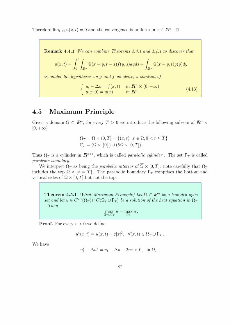
Therefore limt→0 u(x, t) = 0 and the convergence is uniform in x ∈ IRn. 2
Remark 4.4.1 We can combine Theorems 4.3.1 and 4.4.1 to discover that
u(x, t) =
∫ t
0
∫
IRn
Φ(x− y, t− s)f(y, s)dyds+
∫
IRn
Φ(x− y, t)g(y)dy
is, under the hypotheses on g and f as above, a solution of
ut −∆u = f(x, t) in IRn × (0,+∞)u(x, 0) = g(x) in IRn (4.13)
4.5 Maximum Principle
Given a domain Ω ⊂ IRn, for every T > 0 we introduce the following subsets of IRn ×[0,+∞)
ΩT = Ω× (0, T ] = (x, t)| x ∈ Ω, 0 < t ≤ TΓT = (Ω× 0) ∪ (∂Ω × [0, T ]) .
Thus ΩT is a cylinder in IRn+1, which is called parabolic cylinder . The set ΓT is calledparabolic boundary.
We interpret ΩT as being the parabolic interior of Ω × [0, T ]: note carefully that ΩT
includes the top Ω × t = T. The parabolic boundary ΓT comprises the bottom andvertical sides of Ω× [0, T ] but not the top.
Theorem 4.5.1 (Weak Maximum Principle) Let Ω ⊂ IRn be a bounded openset and let u ∈ C2,1(ΩT )∩C(ΩT ∪ΓT ) be a solution of the heat equation in ΩT
. ThenmaxΩT∪ΓT
u = maxΓT
u .
Proof. For every ε > 0 we define
uε(x, t) = u(x, t) + ε|x|2, ∀(x, t) ∈ ΩT ∪ ΓT .
We haveuεt −∆uε = ut −∆u− 2nε < 0, in ΩT .
87

This implies that the maximum of uε cannot be achieved in ΩT . Indeed if (x, t) ∈ ΩT
would be a maximum point for uε then uεt (x, t) ≥ 0 and D2uε(x, t) ≤ 0. In particular∆uε(x, t) ≤ 0 and thus uεt(x, t)−∆uε(x, t) ≥ 0 which is a contradiction. Thus
maxΩT∪ΓT
uε = maxΓT
uε .
It follows that there exists (xε, tε) ∈ ΓT such that
uε(x, t) ≤ uε(xε, tε), ∀(x, t) ∈ ΩT ∪ ΓT .
ThenmaxΩT∪ΓT
u ≤ u(xε, tε) + ε|xε|2 .
Since Γt is compact, there exists a sequence εk → 0 and a point (x, t) such that(xεk , tεk) → (x, t). Hence
maxΩT∪ΓT
u ≤ u(x, t) ≤ maxΓT
u .
Obviously maxΓTu ≤ maxΩT∪ΓT
u and this conclude the proof. 2
4.5.1 Uniqueness of bounded solutions
Theorem 4.5.2 Let g ∈ C(IRn) ∩ L∞(IRn). Then the Cauchy problem
ut −∆u = 0 in IRn × (0,+∞)u(x, 0) = g(x) in IRn (4.14)
has a unique bounded solution.
Proof.Existence: it has already been proved in Theorem 4.3.1.Uniqueness:Step 1. We first show that if u is a bounded solution of (4.14) then
supIRn×(0,+∞)
u(x, t) = supIRn
g(x) .
We set M = supIRn×(0,+∞) u(x, t) and M0 = supIRn g(x) and we define
uε(x, t) = u(x, t) + ε(−2nt− |x|2), ∀(x, t) ∈ IRn × [0,+∞) .
We have uεt −∆uε = 0 and
uε(x, 0) ≤ g(x)− ε|x|2 ≤M0, ∀x ∈ IRn .
88

Moreover for R > 0 large enough we have
sup(x,t)∈∂B(0,R)×[0,R]
uε(x, t) ≤ sup(x,t)∈∂B(0,R)×[0,R]
u(x, t)− εR2
≤ M − εR2 < M0 .
Then by the maximum principle
sup(x,t)∈B(0,R)×(0,R]
uε(x, t) ≤M0
for all R > 0 large enough and thus
uε(x, t) ≤M0, ∀(x, t)IRn × [0,+∞) .
By letting ε → 0 we get the desired estimate.Step 2. Suppose now that u and u be two bounded solution of (4.14). Then v = u− u
is a bounded solution of the Cauchy problemut −∆u = 0 in IRn × (0,+∞)u(x, 0) = 0 in IRn (4.15)
By what it has been proved in Step 1 we get u ≤ u in IRn × (0,+∞) . By arguing in thesame way for the function w = u − u we find that u ≤ u in IRn × (0,+∞) . Therefore uand u coincide. 2
Remark 4.5.1 The uniqueness for the Cauchy problem holds in the class ofbounded functions. Actually one can prove the uniqueness in the class ofunbounded functions satisfying the growth condition |u(x, t)| ≤ Aea|x|
2, with
A, a > 0. This growth condition is necessary. For instance the function (Ty-chonov’s Example)
u(x, t) =
+∞∑
k=0
x2k
(2k)!
dk
dtke−1/t2 , ∀(x, t) ∈ IR× (0,+∞)
is solution of the heat equation and u(x, t) → 0 as t → 0 + . This solutiondiverges as |x| → +∞ much more rapidly as ea|x|
2for every a > 0. Since
v(x, t) = u(x + a, t) is a solution for every a ∈ IR we have that the Cauchyproblem
ut −∆u = 0 in IR× (0,+∞)u(x, 0) = 0 in IR
(4.16)
has infinite solutions.
89

4.6 Mean-value formula
We want to derive a kind of analogous to the mean-value property for harmonic functions.Let us observe that for fixed x the spheres ∂B(x, r) are the level sets of fundamentalsolution Φ(x− y) for Laplace’s equation. This suggests that for fixed (x, t) the level setsof fundamental solution Φ(x− y, t− s) for the heat equation may be relevant.
Definition 4.6.1 For fixed x ∈ IRn, t ∈ IR, r > 0, we define
E(x, t, r) := (y, s) ∈ IRn+1 |s ≤ t,Φ(x− y, t− s) ≥ 1
rn
This is a region in space-time, the boundary of which is a level set of Φ(x− y, t− s).Note that the point (x, t) is at the center of the top.
E(x, t; r) is sometimes called a heat ball.
Theorem 4.6.1 ( A mean-value property for the heat equation) Let Ω ⊂ IRn
be open and let u ∈ C2,1(ΩT ) solve the heat equation. Then
u(x, t) =1
4rn
∫ ∫
E(x,t;r)
u(y, s)|x− y|2(t− s)2
dyds , (4.17)
for each E(x, t; r) ⊆ ΩT .
Formula 4.17 is a sort of analogue for the heat equation of the mean-value formulasfor Laplace’s equation. Observe that the right hand side involves only u(y, s) for timess ≤ t . This is reasonable, as the value u(x, t) should not depend upon future times.
Proof. Up to changing coordinates we may suppose that (x, t) = (0, 0) . We writeE(r) = E(0, 0; r) We set
φ(r) :=1
rn
∫ ∫
E(r)
u(y, s)|y|2s2dyds
=
∫ ∫
E(1)
u(ry, r2s)|y|2s2dyds .
90
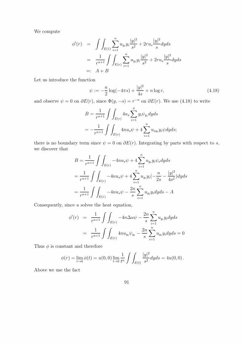
We compute
φ′(r) =
∫ ∫
E(1)
n∑
i=1
uyiyi|y|2s2
+ 2rus|y|2sdyds
=1
rn+1
∫ ∫
E(r)
n∑
i=1
uyiyi|y|2s2
+ 2rus|y|2sdyds
=: A+B
Let us introduce the function
ψ := −n2log(−4πs) +
|y|24s
+ n log r, (4.18)
and observe ψ = 0 on ∂E(r), since Φ(y,−s) = r−n on ∂E(r). We use (4.18) to write
B =1
rn+1
∫ ∫
E(r)
4us
n∑
i=1
yiψyidyds
= − 1
rn+1
∫ ∫
E(r)
4nusψ + 4n∑
i=1
usyiyiψdyds;
there is no boundary term since ψ = 0 on ∂E(r). Integrating by parts with respect to s,we discover that
B =1
rn+1
∫ ∫
E(r)
−4nusψ + 4
n∑
i=1
uyiyiψsdyds
=1
rn+1
∫ ∫
E(r)
−4nusψ + 4n∑
i=1
uyiyi(−n
2s− |y|2
4s2)dyds
=1
rn+1
∫ ∫
E(r)
−4nusψ − 2n
s
n∑
i=1
uyiyidyds− A
Consequently, since u solves the heat equation,
φ′(r) =1
rn+1
∫ ∫
E(r)
−4n∆uψ − 2n
s
n∑
i=1
uyiyidyds
=1
rn+1
∫ ∫
E(r)
4nuyiψyi −2n
s
n∑
i=1
uyiyidyds = 0
Thus φ is constant and therefore
φ(r) = limt→0
φ(t) = u(0, 0) limt→0
1
tn
∫ ∫
E(t)
|y|2s2dyds = 4u(0, 0) .
Above we use the fact
91

1
tn
∫ ∫
E(t)
|y|2s2dyds = 4 ZEXERCISE
2
Figure 4.1: Parabolic Balls of Radius 1 in IR3
92

4.6.1 Strong Maximum Principle for the Heat Equation
Theorem 4.6.2 Let Ω ⊂ IRn be a bounded connected open set. Assume thatu ∈ C2,1(ΩT ) ∩ C(ΩT ) is a solution of the Heat equation such that
u(x0, t0) = maxΩT
u .
Then u is constant in Ωt0 .
Similar assertions are valid with “min” replacing “max”.
Remark 4.6.1 If u attains its maximum (or minimum) at an interior point,then u is constant at earlier times. This accords with our strong intuitive inter-pretation of the variable t as denoting time: the solution will be constant on theinterval [0, t0] provided the initial and the boundary conditions are constant.The solution may change at times t > t0, provided the boundary conditionsalter after t0. The solution will however not respond to changes in boundaryconditions until these changes happen.
Proof.1. Suppose there exists a point (x0, t0) ∈ ΩT with u(x0, t0) = M =: maxΩT
u. Thenfor sufficiently small r > 0, E(x0, t0; r) ⊂ ΩT . We employ the mean-value property todeduce
M = u(x0, t0) =1
4rn
∫ ∫
E(x0,t0;r)
u(y, s)|x0 − y|2(t0 − s)2
dyds ≤M .
Equality holds only if u is identically equal to M within E(x0, t0; r). Consequentlyu(y, s) =M for all (y, s) ∈ E(x0, t0; r) . .
Draw any line segment L in Ω connecting (x0, t0) with some other points (y0, s0) ∈ ΩT
with s < t . Consider
r0 := mins ≥ s : u(x, t) =M, ∀(x, t) ∈ L, s ≤ t ≤ t0.
Since u is continuous, the minimum is attained. Then u(z0, r0) = M for some (z0, r0) ∈L ∩ ΩT and so u ≡ M on E(z0, r0; r) for all sufficiently small r > 0. Since E(z0, r0; r)contains L ∩ r0 − σ ≤ t ≤ r0 for some small σ > 0, we have a contradiction. Thusr0 = s0 and u ≡M on L .
2. Now fix a point (x, t) ∈ Ωt0 . There exist point x0, x1, . . . , xm = x such that theline segments in IRm connecting xi−1 to xi lie in Ω for every i . Select times t0 > t1 >
93
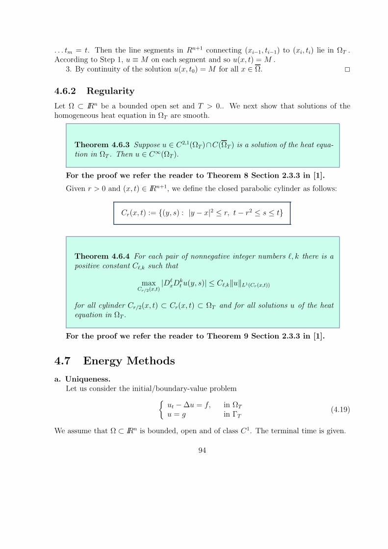
. . . tm = t. Then the line segments in Rn+1 connecting (xi−1, ti−1) to (xi, ti) lie in ΩT .According to Step 1, u ≡M on each segment and so u(x, t) =M .
3. By continuity of the solution u(x, t0) =M for all x ∈ Ω. 2
4.6.2 Regularity
Let Ω ⊂ IRn be a bounded open set and T > 0.. We next show that solutions of thehomogeneous heat equation in ΩT are smooth.
Theorem 4.6.3 Suppose u ∈ C2,1(ΩT )∩C(ΩT ) is a solution of the heat equa-tion in ΩT . Then u ∈ C∞(ΩT ).
For the proof we refer the reader to Theorem 8 Section 2.3.3 in [1].
Given r > 0 and (x, t) ∈ IRn+1, we define the closed parabolic cylinder as follows:
Cr(x, t) := (y, s) : |y − x|2 ≤ r, t− r2 ≤ s ≤ t
Theorem 4.6.4 For each pair of nonnegative integer numbers ℓ, k there is apositive constant Cℓ,k such that
maxCr/2(x,t)
|DℓxD
kt u(y, s)| ≤ Cℓ,k‖u‖L1(Cr(x,t))
for all cylinder Cr/2(x, t) ⊂ Cr(x, t) ⊂ ΩT and for all solutions u of the heatequation in ΩT .
For the proof we refer the reader to Theorem 9 Section 2.3.3 in [1].
4.7 Energy Methods
a. Uniqueness.Let us consider the initial/boundary-value problem
ut −∆u = f, in ΩT
u = g in ΓT(4.19)
We assume that Ω ⊂ IRn is bounded, open and of class C1. The terminal time is given.
94
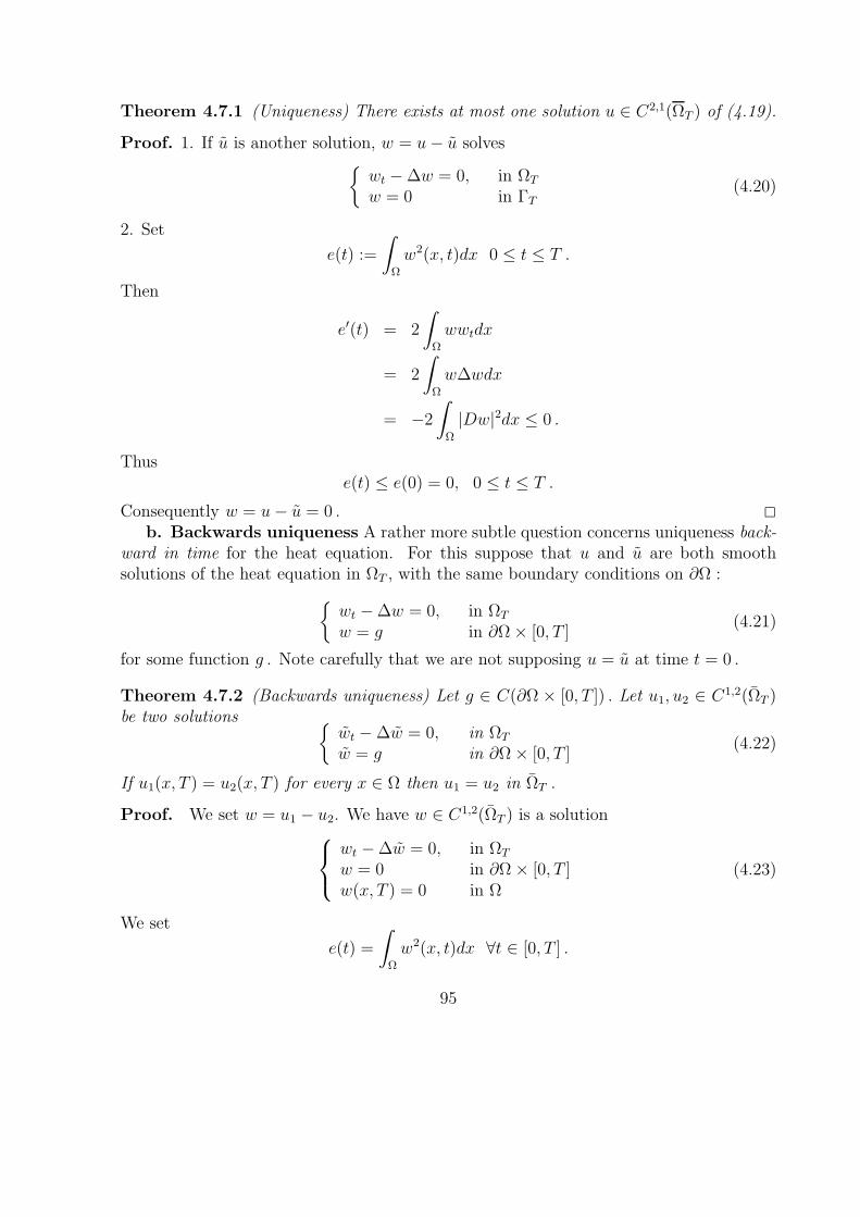
Theorem 4.7.1 (Uniqueness) There exists at most one solution u ∈ C2,1(ΩT ) of (4.19).
Proof. 1. If u is another solution, w = u− u solveswt −∆w = 0, in ΩT
w = 0 in ΓT(4.20)
2. Set
e(t) :=
∫
Ω
w2(x, t)dx 0 ≤ t ≤ T .
Then
e′(t) = 2
∫
Ω
wwtdx
= 2
∫
Ω
w∆wdx
= −2
∫
Ω
|Dw|2dx ≤ 0 .
Thuse(t) ≤ e(0) = 0, 0 ≤ t ≤ T .
Consequently w = u− u = 0 . 2
b. Backwards uniqueness A rather more subtle question concerns uniqueness back-ward in time for the heat equation. For this suppose that u and u are both smoothsolutions of the heat equation in ΩT , with the same boundary conditions on ∂Ω :
wt −∆w = 0, in ΩT
w = g in ∂Ω× [0, T ](4.21)
for some function g . Note carefully that we are not supposing u = u at time t = 0 .
Theorem 4.7.2 (Backwards uniqueness) Let g ∈ C(∂Ω × [0, T ]) . Let u1, u2 ∈ C1,2(ΩT )be two solutions
wt −∆w = 0, in ΩT
w = g in ∂Ω× [0, T ](4.22)
If u1(x, T ) = u2(x, T ) for every x ∈ Ω then u1 = u2 in ΩT .
Proof. We set w = u1 − u2. We have w ∈ C1,2(ΩT ) is a solution
wt −∆w = 0, in ΩT
w = 0 in ∂Ω × [0, T ]w(x, T ) = 0 in Ω
(4.23)
We set
e(t) =
∫
Ω
w2(x, t)dx ∀t ∈ [0, T ] .
95
We have e(t) ≥ 0 for every t ∈ [0, T ], e(T ) = 0 and as we have already seen
e′(t) = −2
∫
Ω
|∇w|2dx .
We compute
e′′(t) = −2
∫
Ω
∂t(|∇w|2)dx = −4
∫
Ω
∇w · ∇wtdx
= 4
∫
Ω
∆w · wtdx− 4
∫
∂Ω
∂w
∂ν· wtdσ(x)
= 4
∫
Ω
|∆w|2dx .
Moreover
(e′(t))2 = 4
(∫
Ω
w∆wdx
)2
≤ e(t)e′′(t) .
Suppose now that there exits t1 ∈ [0, T ] such that e(t1) > 0 . Since e(T ) = 0 it must bet1 < T and there exits t2 ∈ (t1, T ] such that e(t2) = 0 and e(t) > 0 for all t ∈ [t1, t2).For t ∈ [t1, t2) we set f(t) = log(e(t)) and we observe that f ′′(t) ≥ 0. Thus f is convexin [t1, t2). But f(t) → −∞ as t → t−2 which is contradiction. Thus e(t) = 0 for everyt ∈ [0, T ], namely u1 = u2 . 2
96

Bibliography
[1] Evans, Lawrence C. Partial differential equations. Graduate Studies inMathematics, 19. American Mathematical Society, Providence, RI, 1998.
[2] Gilbarg, David; Trudinger, Neil S. Elliptic partial differential equations
of second order. Reprint of the 1998 edition.
[3] Salsa, Sandro. Partial differential equations in action. From modelling totheory. Universitext. Springer-Verlag Italia, Milan, 2008.
97