CHAPTER 4

Introduction to Partial Differential Equations

4.1. Some Examples

Example 4.1. (The one-dimensional heat conduction equation)We consider the heat conduction problem (see Chapter 1) in an (infinitely) thin rod of length

l (see Fig. 4.1.1). Let the heat at the point x and time t be given by u(x, t). Assume that theheat distribution in the rod at the time t = 0 is given by the function f (x), and that the heat at theendpoints x = 0 and x = l are given by the functions h(t) and g(t), respectively (in practice h and gare measured quantities). Then u(x, t) is described by the heat conduction equation:

u′t − ku′′xx = 0, t > 0,0 < x < l,

u(x,0) = f (x), 0 < x < l,

u(0, t) = h(t), t > 0,

u(l, t) = g(t), t > 0.

FIGURE 4.1.1. One-dimensional heat conduction0 l

♦

Example 4.2. (The inhomogeneous one-dimensional heat conduction equation)Suppose that we have the same system as in the previous example, but that we also add the heat

v(x, t) at the point x and time t (see Fig. 4.1.2). In this case u(x, t) is described by the inhomogeneousheat conduction equation:

u′t − ku′′xx = v(x, t), t > 0,0 < x < l,

u(x,0) = f (x), 0 < x < l,

u(0, t) = h(t), t > 0,

u(l, t) = g(t), t > 0.

FIGURE 4.1.2. One-dimensional inhomogeneous heat conduction

0 lx

v = v(x, t)

♦

9

10 4. INTRODUCTION TO PARTIAL DIFFERENTIAL EQUATIONS

Example 4.3. (The two-dimensional inhomogeneous heat conduction equation)We now consider heat conduction in a two-dimensional region D. Let the heat at the point

(x,y) ∈ D at the time t be given by u(x,y, t). Assume that the heat distribution at t = 0 is describedby the function f (x,y), and that the heat at the boundary of D is constant over time and givenby g(x,y) (in practice this is obtained by transfer of heat into or out from the system through theboundary). Assume also that the heat v(x,y, t) is added to the point (x,y) at the time t. Then u(x,y, t)is described by the two-dimensional inhomogeneous heat conduction equation:

u′t − k(u′′xx +u′′yy

)= v(x,y, t), (x,y) ∈ D, t > 0,

u(x,y,0) = f (x,y), (x,y) ∈ D,

u(x,y, t) = g(x,y), (x,y) ∈ ∂D, t > 0.

∂D(x,y)

D

♦

Example 4.4. (The three-dimensional heat conduction equation)We now consider heat conduction in a three-dimensional region V . We use the same notation

as above, with the addition of a z-coordinate. Then u(x,y,z, t) is described by the three-dimensionalheat conduction equation:

u′t −div(kgradu) = v(x,y,z, t), (x,y,z) ∈V, t > 0,(4.1.1)u(x,y,z,0) = f (x,y,z), (x,y,z) ∈V,

u(x,y,z, t) = g(x,y,z), (x,y,z) ∈ ∂V, t > 0.

♦

REMARK 1. Note that the gradient “grad” of the function u(x,y,z) is given by the vector

gradu = ∇u =(u′x,u

′y,u

′z)

=(

∂u∂x

,∂u∂z

,∂u∂z

)=(

∂

∂x,

∂

∂z,

∂

∂z

)u.

If ∇ is written as

∇ =(

∂

∂x,

∂

∂z,

∂

∂z

),

the divergence “div”, of a vector field ~F = (Fx,Fy,Fz) is given by

divF = ∇ ·~F =∂Fx

∂x+

∂Fy

∂z+

∂Fz

∂z.

Thus, the divergence of the gradient of u(x,y,z) is given by

div(gradu) = ∇ ·∇u = ∇2u = ∆u = u′′xx +u′′yy +u′′zz.

Hence, if k = k(x,y,z) = k0 is constant (4.1.1) can be written as

u′t − k0(u′′xx +u′′yy +u′′zz

)= v ⇔ u′t − k0∆u = v.

REMARK 2. Observe that the equationu′t −κ∆u = v

in general describes a diffusion process. Heat conduction implies a diffusion (transport) of heat, and isone example of such a process. Some other examples of diffusion processes are

4.1. SOME EXAMPLES 11

• Mixing of one liquid in another (e.g. milk in a cup of tea).• Diffusion of a gaseous substance in air (e.g. a poisonous gas is released in the air).• Propagation of elementary particles in a solid material (e.g. neutrinos in a nuclear reactor)

Since the equations are the same, all methods we consider here for solving the heat equation in variouscases can also be applied to these alternative diffusion problems. Another PDE which is as important asthe diffusion equation is the wave equation, which we will now consider in some examples of.

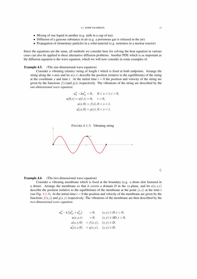
Example 4.5. (The one-dimensional wave equation)Consider a vibrating (elastic) string of length l which is fixed at both endpoints. Arrange the

string along the x-axis and let u(x, t) describe the position (relative to the equilibrium) of the stringat the coordinate x and time t. At the initial time t = 0 the position and velocity of the string aregiven by the functions f (x)and g(x) respectively. The vibrations of the string are described by theone-dimensional wave equation:

u′′tt − ku′′xx = 0, 0 < x < l, t > 0,

u(0, t) = u(l, t) = 0, t > 0,

u(x,0) = f (x),0 < x < l,

u′t(x,0) = g(x), 0 < x < l.

FIGURE 4.1.3. Vibrating string

l0x

u(x, t)

♦

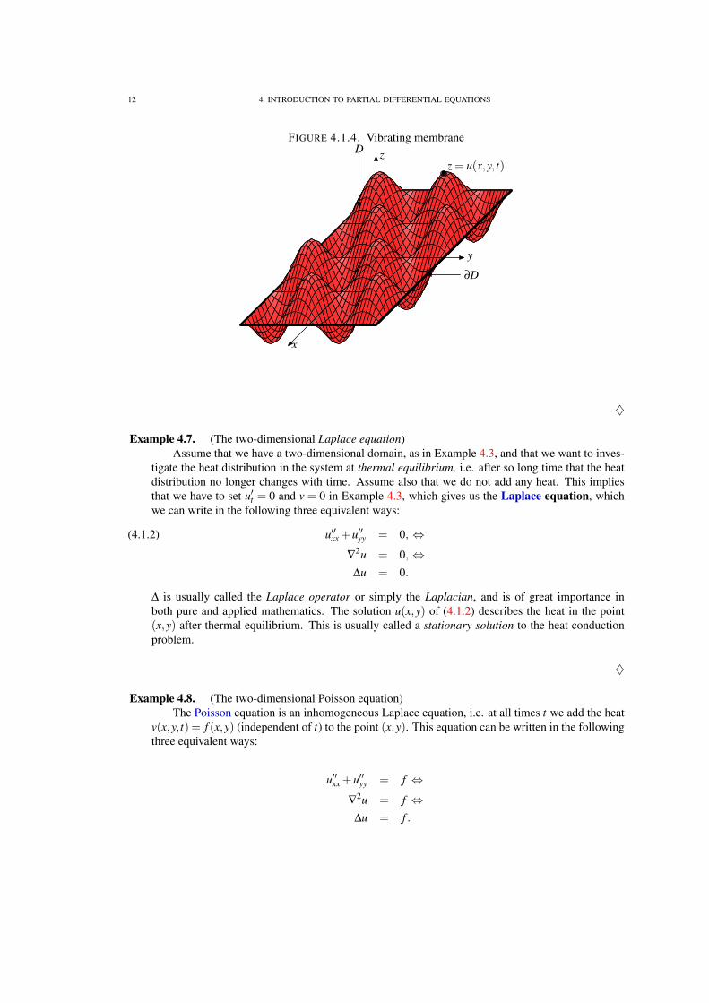
Example 4.6. (The two-dimensional wave equation)Consider a vibrating membrane which is fixed at the boundary (e.g. a drum skin fastened in

a drum). Arrange the membrane so that it covers a domain D in the xy-plane, and let u(x,y, t)describe the position (relative to the equilibrium) of the membrane at the point (x,y) at the time t(see Fig. 4.1.4). At the initial time t = 0 the position and velocity of the membrane are given by thefunctions f (x,y) and g(x,y) respectively. The vibrations of the membrane are then described by thetwo-dimensional wave equation:

u′′tt − k(u′′xx +u′′yy

)= 0, (x,y) ∈ D, t > 0,

u(x,y, t) = 0, (x,y) ∈ ∂D, t > 0,

u(x,y,0) = f (x,y), (x,y) ∈ D,

u′t(x,y,0) = g(x,y), (x,y) ∈ D.

12 4. INTRODUCTION TO PARTIAL DIFFERENTIAL EQUATIONS

FIGURE 4.1.4. Vibrating membrane

x

y

zz = u(x,y, t)

∂D

D

♦

Example 4.7. (The two-dimensional Laplace equation)Assume that we have a two-dimensional domain, as in Example 4.3, and that we want to inves-

tigate the heat distribution in the system at thermal equilibrium, i.e. after so long time that the heatdistribution no longer changes with time. Assume also that we do not add any heat. This impliesthat we have to set u′t = 0 and v = 0 in Example 4.3, which gives us the Laplace equation, whichwe can write in the following three equivalent ways:

u′′xx +u′′yy = 0, ⇔(4.1.2)

∇2u = 0, ⇔∆u = 0.

∆ is usually called the Laplace operator or simply the Laplacian, and is of great importance inboth pure and applied mathematics. The solution u(x,y) of (4.1.2) describes the heat in the point(x,y) after thermal equilibrium. This is usually called a stationary solution to the heat conductionproblem.

♦

Example 4.8. (The two-dimensional Poisson equation)The Poisson equation is an inhomogeneous Laplace equation, i.e. at all times t we add the heat

v(x,y, t) = f (x,y) (independent of t) to the point (x,y). This equation can be written in the followingthree equivalent ways:

u′′xx +u′′yy = f ⇔∇

2u = f ⇔∆u = f .

4.2. A GENERAL PARTIAL DIFFERENTIAL EQUATION OF THE SECOND ORDER 13

Here u′t = 0 and v(x,y, t) =−1k

f (x,y) in Example 4.3, so the the Poisson equation can be interpreted

as the inhomogeneous heat conduction equation at thermal equilibrium (u′t = 0), where we at alltimes t add the heat f (x,y) to the point (x,y).

♦

Example 4.9. (The three-dimensional Poisson equation)

u′′xx +u′′yy +u′′zz = f ⇔∇

2u = f ⇔∆u = f .

In this case we have u′t = 0 and v =− 1k0

f in Example 4.4, and as in the two-dimensional case above,

the three-dimensional Poisson equation can be interpreted as the heat conduction equation at thermal

equilibrium and when at all times t we add the heat − 1k0

f (x,y,z) to the point (x,y,z).

♦

REMARK 3. If the added heat in the examples above have negative sign, the obvious physical interpreta-tion is that we cool down the system.

4.2. A General Partial Differential Equation of the Second Order

A general partial differential equation (PDE) can be written as

(4.2.1) G(x, t,u,u′x,u

′t ,u

′′xx,u

′′xt ,u

′′tt)

= 0.

The basic questions we now ask ourselves are:

1. Does it exist a solution to the PDE?2. Is the solution unique?3. Is the solution stable under small perturbations?4. Which methods are available to construct and illustrate solutions?

Example 4.10. The problems in Examples 4.1-4.6 have unique solutions, but the problems in Example4.7-4.9 do not have unique solutions.

REMARK 4. A PDE of the type (4.2.1) usually has an infinite number of solutions and the general solutiondepends on a number of arbitrary functions (to be compared with the fact that solutions to ODE:s usuallydepend on arbitrary constants).

Example 4.11. The equationu′′tx = tx

has the solutions

u =14

t2x2 +g(t)+h(x).

♦

14 4. INTRODUCTION TO PARTIAL DIFFERENTIAL EQUATIONS

Example 4.12. The two-dimensional Laplace equation

u′′xx +u′′yy = 0,

has, for example, the solutions

u(x,y) = x2− y2,

u(x,y) = ex cosy,

u(x,y) = ln(x2 + y2) .

REMARK 5. A solution u(x,y) to the Laplace equation is called a harmonic function. To find harmonicfunctions one can use the fact that if f (z) = f (x + iy) is an analytic function (or synonymously: entire

or holomorphic), i.e. ifddz

f (z) exists, then the real part u(x,y) = ℜ f (x + iy), and the imaginary part

v(x,y) = ℑ f (x+ iy) of f are both harmonic functions.

In the example above we used f (z) = z2, ez and logz2 respectively.

4.3. Linearity and Non-linearity

A partial differential equation can be written as

(*) Lu = f ,

where L is a so called differential operator.

Example 4.13. Let L =∂

∂t− k

∂2

∂x2 . Then (*) becomes

u′t − ku′′xx = f ,

which is a one-dimensional heat conduction equation (cf. Example 4.2).

♦

Example 4.14. Consider the differential operator

L(u) = u∂u∂t

+2txu.

Then the equation (*) becomes

u∂u∂t

+2txu = f (x, t).

DEFINITION 4.1. We say that the PDE (*) is linear if the operator L has the properties

L(u+ v) = Lu+Lv,(1)

L(cu) = cLu.(2)

If these conditions are not both satisfied we say that (*) is non-linear.

Example 4.15. The heat conduction equation in Example 4.13 is linear.

Proof: We must see verify that L =∂

∂t− k

∂2

∂x2 satisfies (1) and (2) above.

(1) L(u+ v) =∂(u+ v)

∂t− k

∂2(u+ v)∂x2 =

∂u∂t− k

∂2u∂x2 +

∂v∂t− k

∂2v∂x2 = Lu+Lv.

4.4. CLASSIFICATION OF PDES 15

(2) L(cu) =∂(cu)

∂t− k

∂2(cu)∂x2 = c

∂u∂t− kc

∂2u∂x2 = c

(∂u∂t− k

∂2u∂x2

)= cLu.

Hence, since L satisfies both (1) and (2), the equation

Lu = f

is linear. �

Example 4.16. The PDE in Example 4.14 is non-linear.Proof: We start by verifying property (1):

L(u+ v) = (u+ v)(u+ v)′t +2tx(u+ v)= uu′t +uv′t + vu′t + vv′t +2txu+2txv, and

Lu+Lv = uu′t +2txu+ vv′t +2txv.

Since L(u+ v)− (Lu+Lv) = uv′t + vu′t 6= 0 the property (1) is not satisfied and hence the equationis non-linear. �

4.4. Classification of PDEs

A general linear second order PDE can be written as

(4.4.1) a(x, t)u′′tt +b(x, t)u′′xt + c(x, t)u′′xx +d(x, t)u′t + e(x, t)u′x +q(x, t)u = f (x,y), (x, t) ∈D.

SetD(x, t) = (b(x, t))2−4a(x, t)c(x, t).

We say that the PDE (4.4.1) is

• Elliptic if D(x, t) < 0 in D,• Parabolic if D(x, t) = 0 in D,• Hyperbolic if D(x, t) > 0 in D.

Example 4.17. Consider the two-dimensional Laplace equation

u′′xx +u′′yy = 0.

Here D(x,y) = 02−4 ·1 ·1 =−4 < 0, and hence the equation is elliptic.♦

Example 4.18. Consider the heat conduction equation

u′t −u′′xx = 0.

Here D(x,y) = 02−4 ·0 · (−1) = 0, and hence the equation is parabolic.♦

Example 4.19. Consider the one-dimensional wave equation

u′′tt −u′′xx = 0.

Here D(x,y) = 02−4 ·1 · (−1) = 4 > 0, and hence the equation is hyperbolic.

16 4. INTRODUCTION TO PARTIAL DIFFERENTIAL EQUATIONS

4.5. The Superposition Principle

Consider a linear and homogeneous (i.e. the right hand side is 0) PDE:

(*) Lu = 0.

Suppose that u1,u2, . . . are solutions of (*) and that u is a finite linear combination of these:

u = c1u1 + c2u2 + · · ·+ cnun.

Then u is also a solution to (*) since

Lu = L(c1u1 + · · ·+ cnun) = c1Lu1 + · · ·+ cnLun = 0+ · · ·+0 = 0.

This is called the superposition principle and is true also for infinite sums:

u = c1u1 + c2u2 + · · ·+ cnun + · · · ,

provided that certain convergence properties hold1.

The continuous superposition principle:

Assume that uα(x, t) satisfies Luα = 0 for all α, a≤ α≤ b, and define

u(x, t) =Z b

ac(α)uα(x, t)dα,

where c(α) is an arbitrary (integrable) function. Then

Lu = 0.

Proof:

Lu = L(Z b

ac(α)uα(x, t)dα

)=

Z b

ac(α)Luα(x, t)dα

=Z b

ac(α) ·0dα = 0.

�

Example 4.20. It is easy to verify that for each −∞ < α < ∞, the function

uα(x, t) =1√4πkt

exp

(− (x−α)2

4kt

)satisfies the heat conduction equation

u′t − ku′′xx = 0.

Hence this equation is also satisfied by the function

u(x, t) =1√4πkt

Z∞

−∞

c(α)exp(− (x−α)2

4kt

)dα,

for any arbitrary, integrable function c(α).

1E.g. if we have uniform convergence in: sn(x) =n

∑1

u j(x)→ u, s′n(x) =n

∑1

u′j(x)→ u′, etc. for all occurring derivatives.

4.6. WELL-POSED PROBLEMS 17

4.6. Well-Posed Problems

A boundary or initial value problem is said to be well-posed if

(a) there exists a solution,(b) the solution is unique, and(c) the solution is stable.

A problem that is not well-posed is said to be ill-posed.

Example 4.21. Consider the initial-values problem which consists of the equation

u′′tt +u′′xx = 0, t > 0,−∞ < x < ∞,

together with the initial-values

(4.6.1) u(x,0) = 0, u′t(x,0) = 0,−∞ < x < ∞.

The unique solution is given by the function which is constant 0:

u(x, t)≡ 0, t ≥ 0,−∞ < x < ∞.

Let us now make a little perturbation of the initial-values (4.6.1):

(4.6.2) u(x,0) = 0, u′t(x,0) = 10−4 sin104x.

The solution to this new problem is given by

u(x, t) = 10−8 sin(104x

)sinh

(104t

).

For large t we know that sinh(104t

)is approximately

12

exp(104t

). The tiny change in the initial-

values ave rise to a change in the solution from the constant 0 to a function which grows expo-nentially (from the sinh-factor) and oscillates exponentially much (from the sine-factor). A reallydramatic change! This implies that the solution is not stable, and hence the problem is ill-posed.

♦

Example 4.22. Show that the boundary-value problemu′t − ku′′xx = 0, 0 < x < l, 0 < t < T,

u(x,0) = f (x), 0 < x < l,u(0, t) = g(t),u(l, t) = h(t), 0 < t < T,

where f ∈ C [0, l] and g,h ∈ C [0,T ], has a unique solution, u(x, t), in the rectangle

R : 0 ≤ x ≤ l, 0≤ t ≤ T.

Solution: Later on we will construct a solution to this problem (in Example 5.9)!But for now, assume that we have two different solutions to the problem: u1(x, t) and u2(x, t). It

is then clear that the function

w(x, t) = u1(x, t)−u2(x, t)

must satisfy the boundary-value problem:w′

t − kw′′xx = 0, 0 < x < l, 0 < t < T,

w(x,0) = 0, 0 < x < l,w(0, t) = w(l, t) = 0, 0 < t < T.

18 4. INTRODUCTION TO PARTIAL DIFFERENTIAL EQUATIONS

We now form the “energy integral”

E(t) =Z l

0w2(x, t)dx.

Observe that E(t)≥ 0, E(0) = 0, and

E ′(t) =Z l

02ww′

tdx = 2kZ l

0ww′′

xxdx

=[2kww′

x]l

0−2kZ l

0

(w′

x)2 dx

= −2kZ l

0

(w′

x)2 dx ≤ 0.

Hence, the function E is decreasing from E(0) = 0, and since E ≥ 0 we must have E(t) ≡ 0. Thisimplies that also w(x, t) ≡ 0, i.e. u1(x, t) = u2(x, t) for all x, t. Since we assumed that the solutionsu1 and u2 were different we have arrived at a contradiction! Hence the problem must have a uniquesolution! ♦

4.7. Some Remarks On Fourier Series

Consider a function f (x), −l < x < l. The Fourier coefficients of f are defined as

a0 =12l

Z l

−lf (x)dx,

an =1l

Z l

−lf (x)cos

(nπxl

)dx, n = 1,2, . . . ,

bn =1l

Z l

−lf (x)sin

(nπxl

)dx, n = 1,2, . . . ,

and the Fourier series of f is defined by

S(x) = a0 +∞

∑n=1

an cos(nπx

l

)+bn sin

(nπxl

).

For a more detailed discussion of Fourier series see Section 6.1. See also Fig. 4.7.

Assume that f (x) is infinitely many times differentiable in the interval −l < x < l, except for a numberof discontinuity points. Then we have:

(a) S(x) = S(x+2l), for all x.(b) S(x) = f (x) at the points where f is continuous,

(c) S(x) =12

[ f (x+)+ f (x−)] at points of discontinuity2.

2Here f (+x) = limy→x

f (y), where we keep y > x as we take the limit, and we define f (x−) similarly.

4.7. SOME REMARKS ON FOURIER SERIES 19

y

x−l l

f (x)

(a) A Discontinuous Function

y

x−l l

S(x)f (x)

(b) And its Fourier Series

When making a graph of a discontinuous function it is customary to indicate the value which is attainedby the function with a filled circle and the value which is not attained by an unfilled circle.

FIGURE 4.7.1. A square wavey

k

−k

x−π π

f (x) =

{k, 0 < x < l,−k, −l < x≤ 0

Example 4.23. Consider the function f (x) from Fig. 4.7.1:

f (x) =

{k, 0 < x < l,−k, −l < x ≤ 0.

Note that f (x) is odd, i.e. f (−x) = − f (x). Since cosx is even the function f (x)cos(nπx

l

)is

odd and we know that the integral of an odd function over an even interval is always 0 (the “negative”

20 4. INTRODUCTION TO PARTIAL DIFFERENTIAL EQUATIONS

area cancels the “positive” area), hence a0 = an = 0 for all n. And we have

bn =1l

Z l

−lf (x)sin

(nπxl

)dx

=1l

Z 0

−l−k sin

(nπxl

)dx+

Z l

0k sin

(nπxl

)dx

=2kl

Z l

0sin(nπx

l

)dx

=2kl

[− l

nπcos(nπx

l

)]l

0

=2knπ

(1− cosnπ)

=2knπ

(1− (−1)n) .

I.e.

b1 =4kπ

, b2 = 0, b3 =4k3π

, b4 = 0, b5 =4k5π

, . . . ,

and the Fourier series of f is

S(x) =4kπ

∞

∑n=1

bn sin(nπx

l

)=

4kπ

∞

∑m=0

12m+1

sin(

(2m+1)πxl

)=

4kπ

(sin(

πxl

)+

13

sin(

3πxl

)+

15

sin(

5πxl

)+ · · ·

).

See Fig. 4.7.2 for an illustration of some of the partial (containing only a finite number of terms)sums for S(x).

4.8. SEPARATION OF VARIABLES 21

FIGURE 4.7.2. Partial Fourier seriesy

k

−k

xπ π

S1(x)

(a) The First Term

y

k

−k

xπ π

S1(x)4k3π

sin3x4k5π

sin5x

S2(x)

S3(x)

(b) More Terms

4.8. Separation of Variables

Separation of variables is a common method to solve certain types of PDEs. Since it originated from anidea of Fourier it is also sometimes called Fourier’s method.

22 4. INTRODUCTION TO PARTIAL DIFFERENTIAL EQUATIONS

Model example: Solve the problem

u′t − ku′′xx = 0, 0 < x < l, t > 0,(1)

u(x,0) = f (x), 0 < x < l,(2)

u(0, t) = u(l, t) = 0, t > 0.(3)

What we mean by separating the variables in (1) is to seek a solution u(x, t) which can be factored as

u(x, t) = X(x)T (t),

where X(x) and T (t) are functions depending only on x and t respectively. Assume now that we can writeu in this way. If we differentiate u = XT we get u′t(x, t) = X(x)T ′(t) and u′′xx(x, t) = X ′′(x)T (t), and if wesubstitute these expressions into (1) we get the equation:

X(x)T ′(t)− kX ′′(x)T (t) = 0,

which can be rewritten asT ′(t)T (t)

1k

=X ′′(x)X(x)

.

Wee see that the left hand side is a function of t only and the right hand side is a function of x only. Hence,the the only possibility is that both sides equals a constant:

T ′(t)T (t)

1k

=X ′′(x)X(x)

=−λ,

for some constant λ (which we have to determine later). Instead of the PDE (1) we now have two ODEs:{T ′(t) =−λkT (t),X ′′(x) =−λX(x),

with the general solutions

T (t) = Ce−λkt ,and X(x) = Asin(√

λx)

+Bcos(√

λx)

.

The boundary values (3) implies that either T ≡ 0 or X(0) = X(l) = 0. Since the first alternative only givesus the solution which is constant 0 we see that X must satisfy the boundary conditions X(0) = X(l) = 0,i.e.

X(0) = B = 0,

which tells us that B = 0, and we also see that

X(l) = Asin(√

λl)

= 0.

To once again avoid the trivial solution W ≡ 0 (i.e. with A = 0) we must have sin(√

λl)

= 0, whichimplies that √

λl = nπ, n ∈ Z+,

or equivalently

λ =n2π2

l2 ,

for some positive integer n.

We have showed that if a solution to (1) can be factored as X(x)T (t) then it can be written as

K sin(nπ

lx)

exp(−n2π2kt

l2

),

4.8. SEPARATION OF VARIABLES 23

where n is a positive integer and K a constant. By the superposition principle (sec 4.5) the general solutionto (1) satisfying the boundary-values (3) can be written as

u(x, t) =∞

∑n=1

bn sin(nπ

lx)

exp(−n2π2kt

l2

),

where the Fourier coefficients, {bn}∞n=1, are determined by the initial condition (2):

(*) u(x,0) = f (x) =∞

∑n=1

bn sin(nπ

lx)

.

Let us for simplicity assume that l = π and consider some examples of initial values f (x) in the abovemodel example.

Example 4.24. Let f (x) = 2sinx + 4sin3x. Then (*) is satisfied if b1 = 2, b2 = 0, b3 = 4, b4 = b5 =· · ·= 0. Hence, the solution to the model example is

u(x, t) = 2sin(x)e−xt +4sin(3x)e−9kt .

♦

Example 4.25. Let f (x) = 1 =4π

(sinx+

13

sin3x+15

sin5x+ · · ·)

. Then (*) is satisfied if b1 =4π

,

b2 = 0, b3 =4π

13, b4 = 0, b5 =

4π

15, b6 = 0, etc. in this case, the solution to the model example is

given by

u(x, t) =4π

(sin(x)e−kt +

13

sin(3x)e−9kt +15

sin(5x)e−25kt + · · ·)

=4π

∞

∑n=1

sin((2n−1)x)e−(2n−1)2kt .

♦

Example 4.26. If we have an arbitrary initial-value function f (x), 0≤ x≤ π, the solution to the modelexample is given by

u(x, t) =∞

∑n=1

bn sin(nx)exp(−n2kt

),

where

bn =1π

Zπ

−π

fu(x)sinnxdx =2π

Zπ

0f (x)sinnxdx.

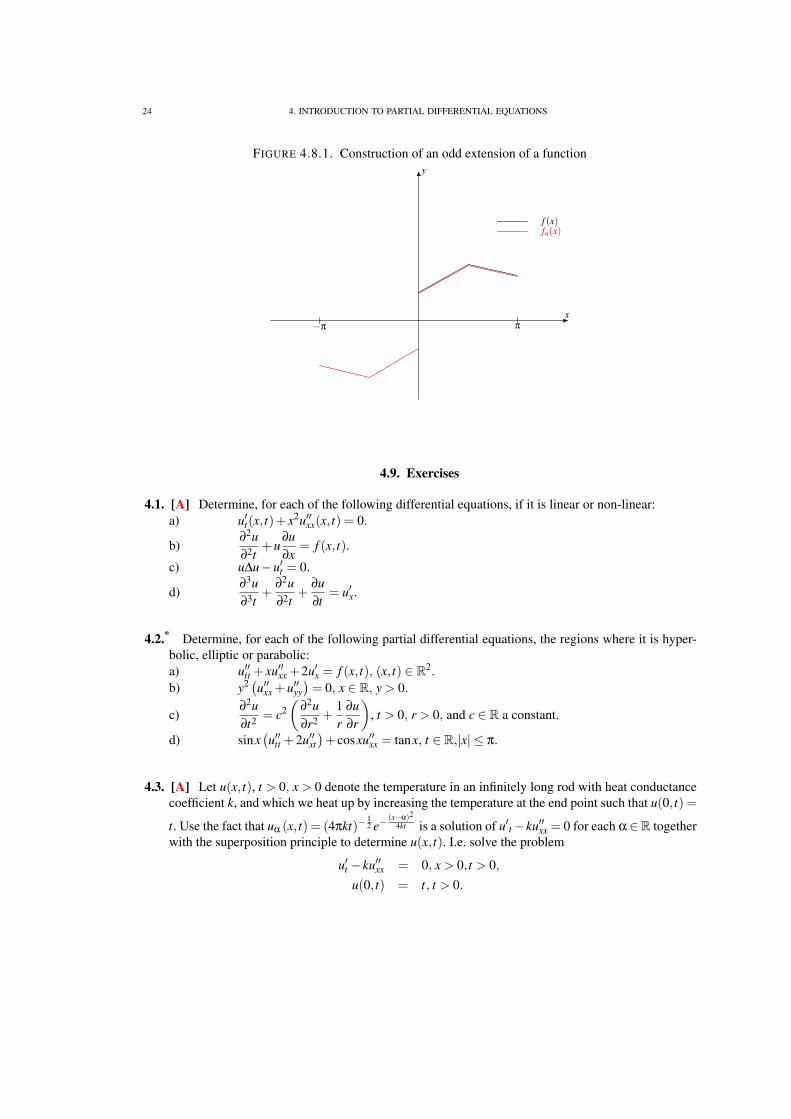
Here fu(x) is an extension of f (x) to an odd function in the interval −π < x < π, i.e. fu(x) = f (x) ifx > 0 and fu(x) =− f (x) if x ≤ 0 (cf. Fig. 4.8.1).

24 4. INTRODUCTION TO PARTIAL DIFFERENTIAL EQUATIONS

FIGURE 4.8.1. Construction of an odd extension of a functiony

x−π π

fu(x)f (x)

4.9. Exercises

4.1. [A] Determine, for each of the following differential equations, if it is linear or non-linear:a) u′t(x, t)+ x2u′′xx(x, t) = 0.

b)∂2u∂2t

+u∂u∂x

= f (x, t).

c) u∆u−u′t = 0.

d)∂3u∂3t

+∂2u∂2t

+∂u∂t

= u′x.

4.2.* Determine, for each of the following partial differential equations, the regions where it is hyper-bolic, elliptic or parabolic:a) u′′tt + xu′′xx +2u′x = f (x, t), (x, t) ∈ R2.b) y2 (u′′xx +u′′yy

)= 0, x ∈ R, y > 0.

c)∂2u∂t2 = c2

(∂2u∂r2 +

1r

∂u∂r

), t > 0, r > 0, and c ∈ R a constant.

d) sinx(u′′tt +2u′′xt

)+ cosxu′′xx = tanx, t ∈ R,|x| ≤ π.

4.3. [A] Let u(x, t), t > 0, x > 0 denote the temperature in an infinitely long rod with heat conductancecoefficient k, and which we heat up by increasing the temperature at the end point such that u(0, t) =

t. Use the fact that uα (x, t) = (4πkt)−12 e−

(x−α)24kt is a solution of u′t −ku′′xx = 0 for each α∈R together

with the superposition principle to determine u(x, t). I.e. solve the problem

u′t − ku′′xx = 0, x > 0, t > 0,

u(0, t) = t, t > 0.

4.9. EXERCISES 25

4.4. Determine whether the following problems are well-posed or ill-posed:a) u′′tt = u′′xx, u(0, t) = u(π, t) = u(x,0) = u(x,π), x, t ∈ [0,π].b) u′t − ku′′xx = 0, u(0, t) = u(π, t) = 0, u(x,0) = sinx, x ∈ [0,π], t > 0.c) u′t − ku′′xx = 0, u(0, t) = 0, u(x,0) = sin

( x2

), x ∈ [0,π], t > 0.

c) u′t − ku′′xx = 0, u(0, t) = u(π, t) = 0, u(x,0) = sin( x

2

), x ∈ [0,π], t > 0.

4.5. [A] a) Determine the Fourier series for the function f (x) which in the interval −π < x < π is givenby f (x) = x2.

b) use a) to show thatπ2

12=−

∞

∑k=1

(−1)k

k2 .

4.6.* Determine the Fourier series of f (t) = |sin t|.

4.7. [A] Consider a rod of length L = 1 with heat conduction coefficient k = 1. At the beginning therod has the constant temperature 1. We then (instantaneous) cool down the ends of the rod to thetemperature 0, where we then keep it during the continuation of the experiment.a) Formulate this problem mathematically.b) find an expression for the temperature of the rod in the point x at the time t.

(Hint: for the Fourier series expansion of the constant 1 use an odd periodic extensionin the interval.)

4.8.* Solve the following problem by separation of variables:

u′t = u′′xx, 0 < x < 3, t > 0,

u(x,0) = sin(πx)−2sin(

4π

3x)

, 0 < x < 3,

u(0, t) = u(3, t) = 0, t > 0.

4.9. [A] Solve the following problem

u′t = u′′xx, 0 < x < π, t > 0,

u(x,0) = sin2 x, 0 < x < π,

u′x(0, t) = u′x(π, t) = 0, t > 0.

4.10. Solve the following problem

u′′tt = u′′xx, 0 < x < π, t > 0,

u(x,0) = sinx, 0 < x < π,

u′t(x,0) = 1, 0 < x < π,

u(0, t) = u(π, t) = 0, t > 0.