introduction to photogrammetry - gis resources · lps project manager introduction / 15...
TRANSCRIPT
Introduction / 15LPS Project Manager
Introduction to Photogrammetry
Introduction
What is Photogrammetry?
Photogrammetry is the “art, science and technology of obtaining reliable information about physical objects and the environment through the process of recording, measuring and interpreting photographic images and patterns of electromagnetic radiant imagery and other phenomena” (American Society of Photogrammetry 1980).
Photogrammetry was invented in 1851 by Colonel Aimé Laussedat, and has continued to develop over the last 150 years. Over time, the development of photogrammetry has passed through the phases of plane table photogrammetry, analog photogrammetry, analytical photogrammetry, and has now entered the phase of digital photogrammetry (Konecny 1994).
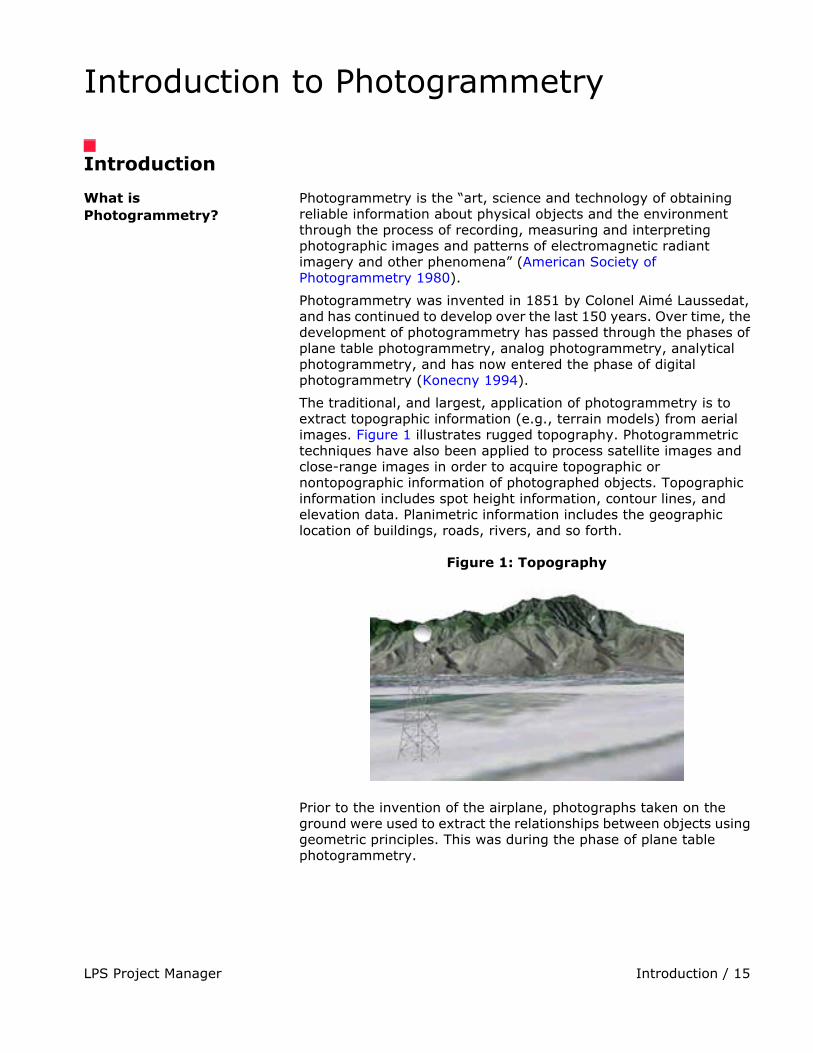
The traditional, and largest, application of photogrammetry is to extract topographic information (e.g., terrain models) from aerial images. Figure 1 illustrates rugged topography. Photogrammetric techniques have also been applied to process satellite images and close-range images in order to acquire topographic or nontopographic information of photographed objects. Topographic information includes spot height information, contour lines, and elevation data. Planimetric information includes the geographic location of buildings, roads, rivers, and so forth.
Figure 1: Topography
Prior to the invention of the airplane, photographs taken on the ground were used to extract the relationships between objects using geometric principles. This was during the phase of plane table photogrammetry.
Introduction / 16LPS Project Manager
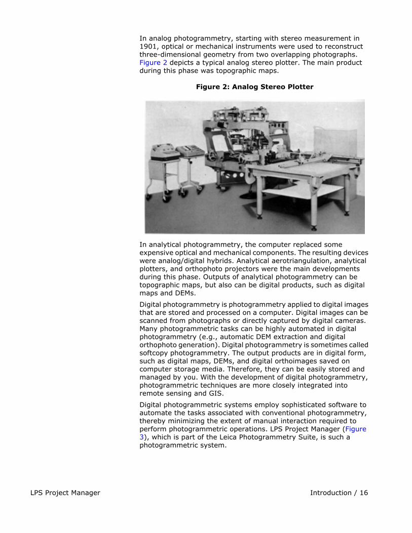
In analog photogrammetry, starting with stereo measurement in 1901, optical or mechanical instruments were used to reconstruct three-dimensional geometry from two overlapping photographs. Figure 2 depicts a typical analog stereo plotter. The main product during this phase was topographic maps.
Figure 2: Analog Stereo Plotter
In analytical photogrammetry, the computer replaced some expensive optical and mechanical components. The resulting devices were analog/digital hybrids. Analytical aerotriangulation, analytical plotters, and orthophoto projectors were the main developments during this phase. Outputs of analytical photogrammetry can be topographic maps, but also can be digital products, such as digital maps and DEMs.
Digital photogrammetry is photogrammetry applied to digital images that are stored and processed on a computer. Digital images can be scanned from photographs or directly captured by digital cameras. Many photogrammetric tasks can be highly automated in digital photogrammetry (e.g., automatic DEM extraction and digital orthophoto generation). Digital photogrammetry is sometimes called softcopy photogrammetry. The output products are in digital form, such as digital maps, DEMs, and digital orthoimages saved on computer storage media. Therefore, they can be easily stored and managed by you. With the development of digital photogrammetry, photogrammetric techniques are more closely integrated into remote sensing and GIS.
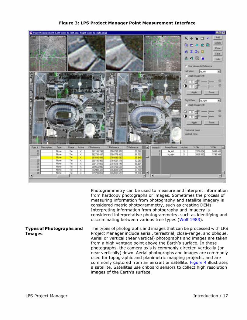
Digital photogrammetric systems employ sophisticated software to automate the tasks associated with conventional photogrammetry, thereby minimizing the extent of manual interaction required to perform photogrammetric operations. LPS Project Manager (Figure 3), which is part of the Leica Photogrammetry Suite, is such a photogrammetric system.
LPS Project Manager Introduction / 17
Figure 3: LPS Project Manager Point Measurement Interface
Photogrammetry can be used to measure and interpret information from hardcopy photographs or images. Sometimes the process of measuring information from photography and satellite imagery is considered metric photogrammetry, such as creating DEMs. Interpreting information from photography and imagery is considered interpretative photogrammetry, such as identifying and discriminating between various tree types (Wolf 1983).
Types of Photographs and Images
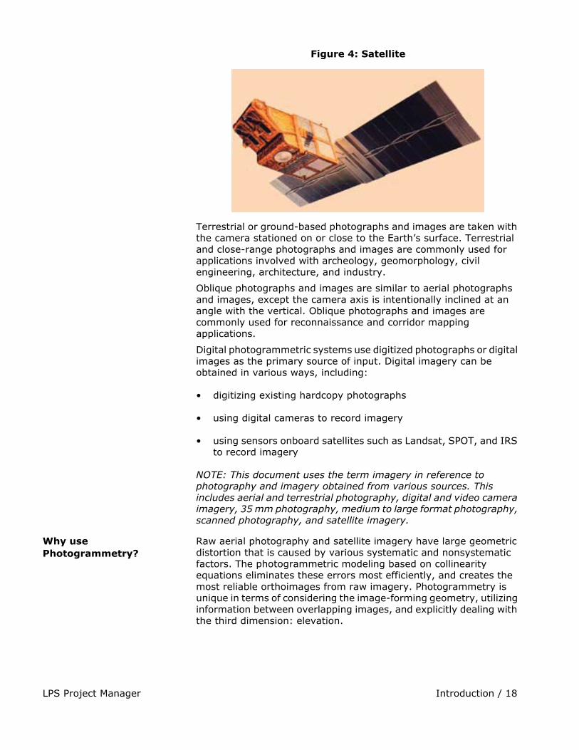
The types of photographs and images that can be processed with LPS Project Manager include aerial, terrestrial, close-range, and oblique. Aerial or vertical (near vertical) photographs and images are taken from a high vantage point above the Earth’s surface. In those photographs, the camera axis is commonly directed vertically (or near vertically) down. Aerial photographs and images are commonly used for topographic and planimetric mapping projects, and are commonly captured from an aircraft or satellite. Figure 4 illustrates a satellite. Satellites use onboard sensors to collect high resolution images of the Earth’s surface.
Introduction / 18LPS Project Manager
Figure 4: Satellite
Terrestrial or ground-based photographs and images are taken with the camera stationed on or close to the Earth’s surface. Terrestrial and close-range photographs and images are commonly used for applications involved with archeology, geomorphology, civil engineering, architecture, and industry.
Oblique photographs and images are similar to aerial photographs and images, except the camera axis is intentionally inclined at an angle with the vertical. Oblique photographs and images are commonly used for reconnaissance and corridor mapping applications.
Digital photogrammetric systems use digitized photographs or digital images as the primary source of input. Digital imagery can be obtained in various ways, including:
• digitizing existing hardcopy photographs
• using digital cameras to record imagery
• using sensors onboard satellites such as Landsat, SPOT, and IRS to record imagery
NOTE: This document uses the term imagery in reference to photography and imagery obtained from various sources. This includes aerial and terrestrial photography, digital and video camera imagery, 35 mm photography, medium to large format photography, scanned photography, and satellite imagery.
Why use Photogrammetry?
Raw aerial photography and satellite imagery have large geometric distortion that is caused by various systematic and nonsystematic factors. The photogrammetric modeling based on collinearity equations eliminates these errors most efficiently, and creates the most reliable orthoimages from raw imagery. Photogrammetry is unique in terms of considering the image-forming geometry, utilizing information between overlapping images, and explicitly dealing with the third dimension: elevation.

LPS Project Manager Introduction / 19
See “The Collinearity Equation” for information about the collinearity equation.
In addition to orthoimages, photogrammetry can also reliably and efficiently provide other geographic information such as a DEM, topographic features, and line maps. In essence, photogrammetry produces accurate and precise geographic information from a wide range of photographs and images. Any measurement taken on a photogrammetrically processed photograph or image reflects a measurement taken on the ground. Rather than constantly go to the field to measure distances, areas, angles, and point positions on the Earth’s surface, photogrammetric tools allow for the accurate collection of information from imagery. Photogrammetric approaches for collecting geographic information save time and money, and maintain the highest accuracy.
Photogrammetry vs. Conventional Geometric Correction
Conventional techniques of geometric correction such as polynomial transformation are based on general functions not directly related to the specific distortion or error sources. They have been successful in the field of remote sensing and GIS applications, especially when dealing with low resolution and narrow field of view satellite imagery such as Landsat and SPOT data (Yang 1997). General functions have the advantage of simplicity. They can provide a reasonable geometric modeling alternative when little is known about the geometric nature of the image data.
Because conventional techniques generally process the images one at a time, they cannot provide an integrated solution for multiple images or photographs simultaneously and efficiently. It is very difficult, if not impossible, for conventional techniques to achieve a reasonable accuracy without a great number of GCPs when dealing with large-scale imagery, images having severe systematic and/or nonsystematic errors, and images covering rough terrain. Misalignment is more likely to occur when mosaicking separately rectified images. This misalignment could result in inaccurate geographic information being collected from the rectified images. Furthermore, it is impossible for a conventional technique to create a 3D stereo model or to extract the elevation information from two overlapping images. There is no way for conventional techniques to accurately derive geometric information about the sensor that captured the imagery.
The photogrammetric techniques applied in LPS Project Manager overcome all the problems of conventional geometric correction by using least squares bundle block adjustment. This solution is integrated and accurate.
For more information, see “Bundle Block Adjustment”.
Introduction / 20LPS Project Manager
LPS Project Manager can process hundreds of images or photographs with very few GCPs, while at the same time eliminating the misalignment problem associated with creating image mosaics. In short: less time, less money, less manual effort, and more geographic fidelity can be obtained using the photogrammetric solution.
Single Frame Orthorectification vs. Block Triangulation
Single Frame Orthorectification
Single frame orthorectification techniques orthorectify one image at a time using a technique known as space resection. In this respect, a minimum of three GCPs is required for each image. For example, in order to orthorectify 50 aerial photographs, a minimum of 150 GCPs is required. This includes manually identifying and measuring each GCP for each image individually. Once the GCPs are measured, space resection techniques compute the camera/sensor position and orientation as it existed at the time of data capture. This information, along with a DEM, is used to account for the negative impacts associated with geometric errors. Additional variables associated with systematic error are not considered.
Single frame orthorectification techniques do not use the internal relationship between adjacent images in a block to minimize and distribute the errors commonly associated with GCPs, image measurements, DEMs, and camera/sensor information. Therefore, during the mosaic procedure, misalignment between adjacent images is common since error has not been minimized and distributed throughout the block.
Block Triangulation
Block (or aerial) triangulation is the process of establishing a mathematical relationship between the images contained in a project, the camera or sensor model, and the ground. The information resulting from aerial triangulation is required as input for the orthorectification, DEM creation, and stereopair creation processes. The term aerial triangulation is commonly used when processing aerial photography and imagery. The term block triangulation, or simply triangulation, is used when processing satellite imagery. The techniques differ slightly as a function of the type of imagery being processed.
LPS Project Manager Introduction / 21
Classic aerial triangulation using optical-mechanical analog and analytical stereo plotters is primarily used for the collection of GCPs using a technique known as control point extension. Since collecting GCPs is time consuming, photogrammetric techniques are accepted as the ideal approach for collecting GCPs over large areas using photography rather than conventional ground surveying techniques. Control point extension involves the manual photo measurement of ground points appearing on overlapping images. These ground points are commonly referred to as tie points. Once the points are measured, the ground coordinates associated with the tie points can be determined using photogrammetric techniques employed by analog or analytical stereo plotters. These points are then referred to as ground control points (GCPs).
With the advent of digital photogrammetry, classic aerial triangulation has been extended to provide greater functionality. LPS Project Manager uses a mathematical technique known as bundle block adjustment for aerial triangulation. Bundle block adjustment provides three primary functions:
• Bundle block adjustment determines the position and orientation for each image in a project as they existed at the time of photographic or image exposure. The resulting parameters are referred to as exterior orientation parameters. In order to estimate the exterior orientation parameters, a minimum of three GCPs is required for the entire block, regardless of how many images are contained within the project.
• Bundle block adjustment determines the ground coordinates of any tie points manually or automatically measured on the overlap areas of multiple images. The highly precise ground point determination of tie points is useful for generating control points from imagery in lieu of ground surveying techniques. Additionally, if a large number of ground points is generated, then a DEM can be interpolated using the 3D surfacing tool in ERDAS IMAGINE.
• Bundle block adjustment minimizes and distributes the errors associated with the imagery, image measurements, GCPs, and so forth. The bundle block adjustment processes information from an entire block of imagery in one simultaneous solution (i.e., a bundle) using statistical techniques (i.e., adjustment component) to automatically identify, distribute, and remove error.
Because the images are processed in one step, the misalignment issues associated with creating mosaics are resolved.
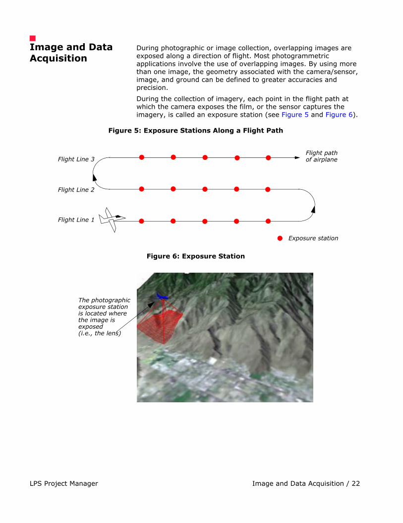
Image and Data Acquisition / 22LPS Project Manager
Image and Data Acquisition
During photographic or image collection, overlapping images are exposed along a direction of flight. Most photogrammetric applications involve the use of overlapping images. By using more than one image, the geometry associated with the camera/sensor, image, and ground can be defined to greater accuracies and precision.
During the collection of imagery, each point in the flight path at which the camera exposes the film, or the sensor captures the imagery, is called an exposure station (see Figure 5 and Figure 6).
Figure 5: Exposure Stations Along a Flight Path
Figure 6: Exposure Station
Flight pathof airplane
Exposure station
Flight Line 1
Flight Line 2
Flight Line 3
The photographicexposure stationis located wherethe image isexposed (i.e., the lens)
LPS Project Manager Image and Data Acquisition / 23
Each photograph or image that is exposed has a corresponding image scale (SI) associated with it. The SI expresses the average ratio between a distance in the image and the same distance on the ground. It is computed as focal length divided by the flying height above the mean ground elevation. For example, with a flying height of 1000 m and a focal length of 15 cm, the SI would be 1:6667.
NOTE: The flying height above ground is used to determine SI, versus the altitude above sea level.
A strip of photographs consists of images captured along a flight line, normally with an overlap of 60%. All photos in the strip are assumed to be taken at approximately the same flying height and with a constant distance between exposure stations. Camera tilt relative to the vertical is assumed to be minimal.
The photographs from several flight paths can be combined to form a block of photographs. A block of photographs consists of a number of parallel strips, normally with a sidelap of 20-30%. Block triangulation techniques are used to transform all of the images in a block and their associated ground points into a homologous coordinate system.
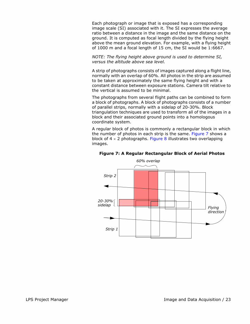
A regular block of photos is commonly a rectangular block in which the number of photos in each strip is the same. Figure 7 shows a block of 4 � 2 photographs. Figure 8 illustrates two overlapping images.
Figure 7: A Regular Rectangular Block of Aerial Photos
Flying
Strip 2
Strip 1
60% overlap
20-30% sidelap
direction
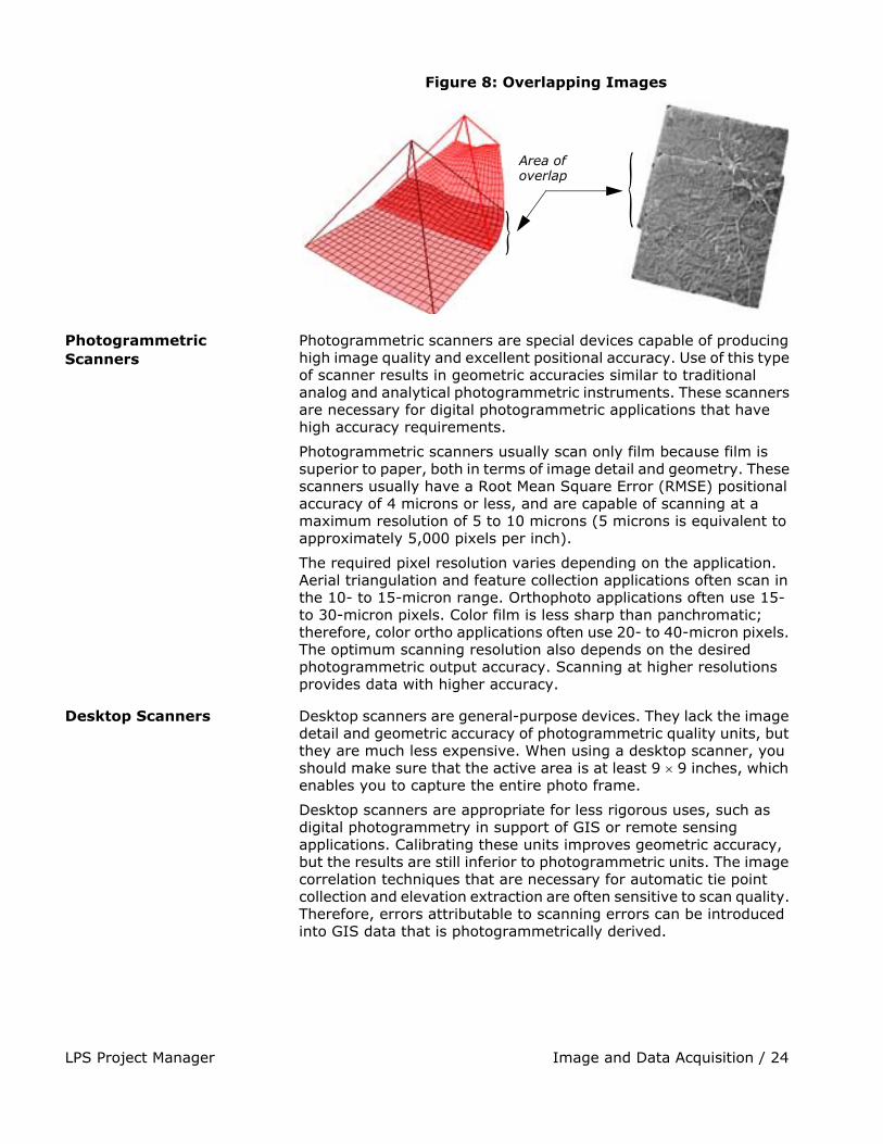
Image and Data Acquisition / 24LPS Project Manager
Figure 8: Overlapping Images
Photogrammetric Scanners
Photogrammetric scanners are special devices capable of producing high image quality and excellent positional accuracy. Use of this type of scanner results in geometric accuracies similar to traditional analog and analytical photogrammetric instruments. These scanners are necessary for digital photogrammetric applications that have high accuracy requirements.
Photogrammetric scanners usually scan only film because film is superior to paper, both in terms of image detail and geometry. These scanners usually have a Root Mean Square Error (RMSE) positional accuracy of 4 microns or less, and are capable of scanning at a maximum resolution of 5 to 10 microns (5 microns is equivalent to approximately 5,000 pixels per inch).
The required pixel resolution varies depending on the application. Aerial triangulation and feature collection applications often scan in the 10- to 15-micron range. Orthophoto applications often use 15- to 30-micron pixels. Color film is less sharp than panchromatic; therefore, color ortho applications often use 20- to 40-micron pixels. The optimum scanning resolution also depends on the desired photogrammetric output accuracy. Scanning at higher resolutions provides data with higher accuracy.
Desktop Scanners Desktop scanners are general-purpose devices. They lack the image detail and geometric accuracy of photogrammetric quality units, but they are much less expensive. When using a desktop scanner, you should make sure that the active area is at least 9 � 9 inches, which enables you to capture the entire photo frame.
Desktop scanners are appropriate for less rigorous uses, such as digital photogrammetry in support of GIS or remote sensing applications. Calibrating these units improves geometric accuracy, but the results are still inferior to photogrammetric units. The image correlation techniques that are necessary for automatic tie point collection and elevation extraction are often sensitive to scan quality. Therefore, errors attributable to scanning errors can be introduced into GIS data that is photogrammetrically derived.
Area of
}{overlap

LPS Project Manager Image and Data Acquisition / 25
Scanning Resolutions One of the primary factors contributing to the overall accuracy of block triangulation and orthorectification is the resolution of the imagery being used. Image resolution is commonly determined by the scanning resolution (if film photography is being used), or by the pixel resolution of the sensor.
In order to optimize the attainable accuracy of a solution, the scanning resolution must be considered. The appropriate scanning resolution is determined by balancing the accuracy requirements versus the size of the mapping project and the time required to process the project.
Table 3 lists the scanning resolutions associated with various scales of photography and image file size.
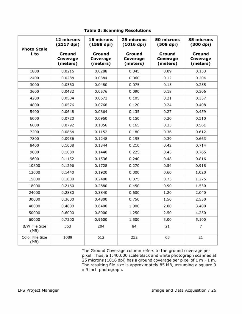
Image and Data Acquisition / 26LPS Project Manager
The Ground Coverage column refers to the ground coverage per pixel. Thus, a 1:40,000 scale black and white photograph scanned at 25 microns (1016 dpi) has a ground coverage per pixel of 1 m � 1 m. The resulting file size is approximately 85 MB, assuming a square 9 � 9 inch photograph.
Table 3: Scanning Resolutions
Photo Scale1 to
12 microns (2117 dpi)
Ground Coverage (meters)
16 microns (1588 dpi)
Ground Coverage (meters)
25 microns (1016 dpi)
Ground Coverage (meters)
50 microns (508 dpi)
Ground Coverage (meters)
85 microns (300 dpi)
Ground Coverage (meters)
1800 0.0216 0.0288 0.045 0.09 0.153
2400 0.0288 0.0384 0.060 0.12 0.204
3000 0.0360 0.0480 0.075 0.15 0.255
3600 0.0432 0.0576 0.090 0.18 0.306
4200 0.0504 0.0672 0.105 0.21 0.357
4800 0.0576 0.0768 0.120 0.24 0.408
5400 0.0648 0.0864 0.135 0.27 0.459
6000 0.0720 0.0960 0.150 0.30 0.510
6600 0.0792 0.1056 0.165 0.33 0.561
7200 0.0864 0.1152 0.180 0.36 0.612
7800 0.0936 0.1248 0.195 0.39 0.663
8400 0.1008 0.1344 0.210 0.42 0.714
9000 0.1080 0.1440 0.225 0.45 0.765
9600 0.1152 0.1536 0.240 0.48 0.816
10800 0.1296 0.1728 0.270 0.54 0.918
12000 0.1440 0.1920 0.300 0.60 1.020
15000 0.1800 0.2400 0.375 0.75 1.275
18000 0.2160 0.2880 0.450 0.90 1.530
24000 0.2880 0.3840 0.600 1.20 2.040
30000 0.3600 0.4800 0.750 1.50 2.550
40000 0.4800 0.6400 1.000 2.00 3.400
50000 0.6000 0.8000 1.250 2.50 4.250
60000 0.7200 0.9600 1.500 3.00 5.100
B/W File Size (MB)
363 204 84 21 7
Color File Size (MB)
1089 612 252 63 21
LPS Project Manager Image and Data Acquisition / 27
Coordinate Systems Conceptually, photogrammetry involves establishing the relationship between the camera or sensor used to capture the imagery, the imagery itself, and the ground. In order to understand and define this relationship, each of the three variables associated with the relationship must be defined with respect to a coordinate space and coordinate system.
Pixel Coordinate System
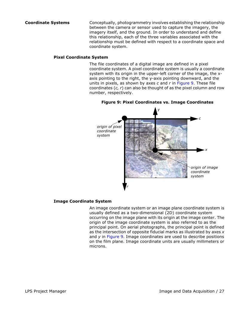
The file coordinates of a digital image are defined in a pixel coordinate system. A pixel coordinate system is usually a coordinate system with its origin in the upper-left corner of the image, the x-axis pointing to the right, the y-axis pointing downward, and the units in pixels, as shown by axes c and r in Figure 9. These file coordinates (c, r) can also be thought of as the pixel column and row number, respectively.
Figure 9: Pixel Coordinates vs. Image Coordinates
Image Coordinate System
An image coordinate system or an image plane coordinate system is usually defined as a two-dimensional (2D) coordinate system occurring on the image plane with its origin at the image center. The origin of the image coordinate system is also referred to as the principal point. On aerial photographs, the principal point is defined as the intersection of opposite fiducial marks as illustrated by axes x and y in Figure 9. Image coordinates are used to describe positions on the film plane. Image coordinate units are usually millimeters or microns.
y
x
c
r
origin of pixel
origin of image
coordinatesystem
coordinatesystem
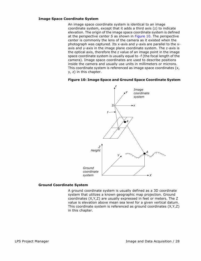
Image and Data Acquisition / 28LPS Project Manager
Image Space Coordinate System
An image space coordinate system is identical to an image coordinate system, except that it adds a third axis (z) to indicate elevation. The origin of the image space coordinate system is defined at the perspective center S as shown in Figure 10. The perspective center is commonly the lens of the camera as it existed when the photograph was captured. Its x-axis and y-axis are parallel to the x-axis and y-axis in the image plane coordinate system. The z-axis is the optical axis, therefore the z value of an image point in the image space coordinate system is usually equal to -f (the focal length of the camera). Image space coordinates are used to describe positions inside the camera and usually use units in millimeters or microns. This coordinate system is referenced as image space coordinates (x, y, z) in this chapter.
Figure 10: Image Space and Ground Space Coordinate System
Ground Coordinate System
A ground coordinate system is usually defined as a 3D coordinate system that utilizes a known geographic map projection. Ground coordinates (X,Y,Z) are usually expressed in feet or meters. The Z value is elevation above mean sea level for a given vertical datum. This coordinate system is referenced as ground coordinates (X,Y,Z) in this chapter.
z
y
x
Image
S
f
a
o
ZHeight
YA
Ground
X
coordinate system
coordinate system
LPS Project Manager Image and Data Acquisition / 29
Geocentric and Topocentric Coordinate System
Most photogrammetric applications account for the Earth’s curvature in their calculations. This is done by adding a correction value or by computing geometry in a coordinate system that includes curvature. Two such systems are geocentric and topocentric.
A geocentric coordinate system has its origin at the center of the Earth ellipsoid. The Z-axis equals the rotational axis of the Earth, and the X-axis passes through the Greenwich meridian. The Y-axis is perpendicular to both the Z-axis and X-axis, so as to create a three-dimensional coordinate system that follows the right hand rule.
A topocentric coordinate system has its origin at the center of the image projected on the Earth ellipsoid. The three perpendicular coordinate axes are defined on a tangential plane at this center point. The plane is called the reference plane or the local datum. The x-axis is oriented eastward, the y-axis northward, and the z-axis is vertical to the reference plane (up).
For simplicity of presentation, the remainder of this chapter does not explicitly reference geocentric or topocentric coordinates. Basic photogrammetric principles can be presented without adding this additional level of complexity.
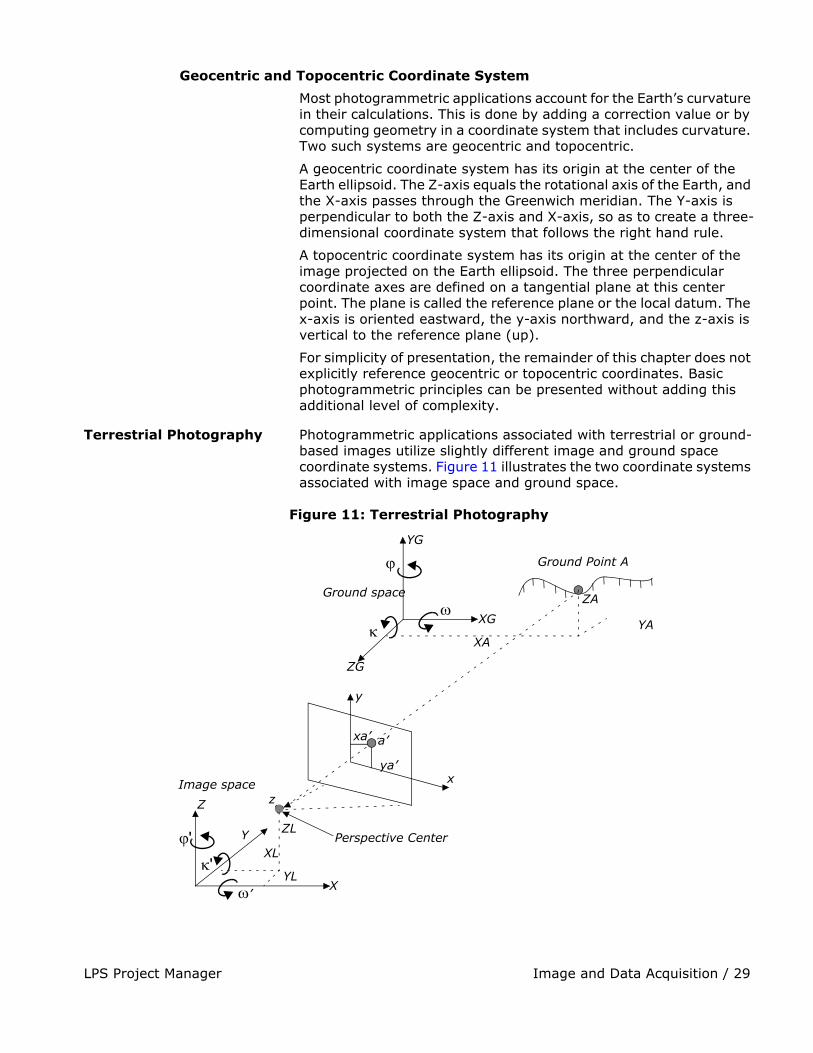
Terrestrial Photography Photogrammetric applications associated with terrestrial or ground-based images utilize slightly different image and ground space coordinate systems. Figure 11 illustrates the two coordinate systems associated with image space and ground space.
Figure 11: Terrestrial Photography
�
�’�
�
�
YG
XG
ZG
XA
ZA
YA
y
x
xa’ a’
ya’
z
Perspective Center
X
Z
ZLYXL
YL
�'�'
Ground space
Ground Point A
Image space
Interior Orientation / 30LPS Project Manager
The image and ground space coordinate systems are right-handed coordinate systems. Most terrestrial applications use a ground space coordinate system that was defined using a localized Cartesian coordinate system.
The image space coordinate system directs the z-axis toward the imaged object and the y-axis directed north up. The image x-axis is similar to that used in aerial applications. The XL, YL, and ZL coordinates define the position of the perspective center as it existed at the time of image capture. The ground coordinates of Ground Point A (XA, YA, and ZA) are defined within the ground space coordinate system (XG, YG, and ZG).
With this definition, the rotation angles ���Omega)����(Phi)��and���(Kappa)�are still defined as in the aerial photography conventions. In LPS Project Manager, you can also use the ground (X, Y, Z) coordinate system to directly define GCPs. Thus, GCPs do not need to be transformed. Then the definition of rotation angles �'���'� and��' is different, as shown in Figure 11.
Interior Orientation
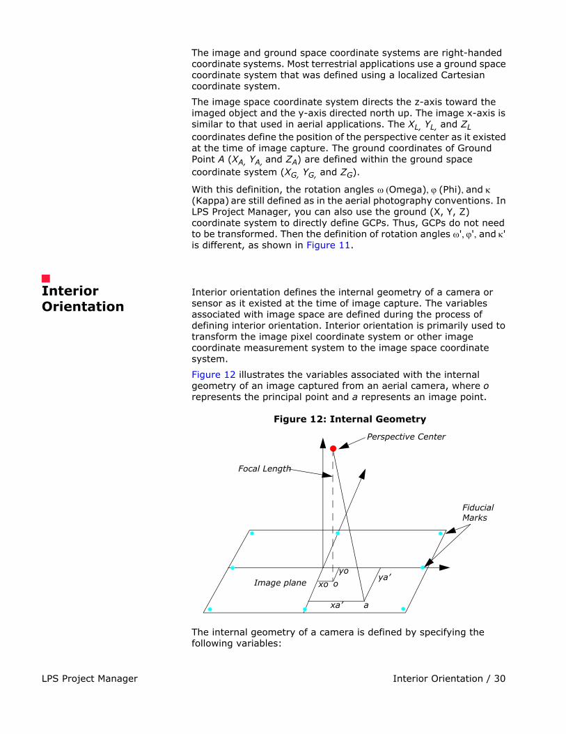
Interior orientation defines the internal geometry of a camera or sensor as it existed at the time of image capture. The variables associated with image space are defined during the process of defining interior orientation. Interior orientation is primarily used to transform the image pixel coordinate system or other image coordinate measurement system to the image space coordinate system.
Figure 12 illustrates the variables associated with the internal geometry of an image captured from an aerial camera, where o represents the principal point and a represents an image point.
Figure 12: Internal Geometry
The internal geometry of a camera is defined by specifying the following variables:
Focal Length
Perspective Center
Fiducial
Image planeyo
xo oya’
xa’ a
Marks
LPS Project Manager Interior Orientation / 31
• principal point
• focal length
• fiducial marks
• lens distortion
Principal Point and Focal Length
The principal point is mathematically defined as the intersection of the perpendicular line through the perspective center of the image plane. The length from the principal point to the perspective center is called the focal length (Wang, Z. 1990).
The image plane is commonly referred to as the focal plane. For wide-angle aerial cameras, the focal length is approximately 152 mm, or 6 in. For some digital cameras, the focal length is 28 mm. Prior to conducting photogrammetric projects, the focal length of a metric camera is accurately determined or calibrated in a laboratory environment.
This mathematical definition is the basis of triangulation, but difficult to determine optically. The optical definition of principal point is the image position where the optical axis intersects the image plane. In the laboratory, this is calibrated in two forms: principal point of autocollimation and principal point of symmetry, which can be seen from the camera calibration report. Most applications prefer to use the principal point of symmetry since it can best compensate for any lens distortion.
Fiducial Marks One of the steps associated with calculating interior orientation involves determining the image position of the principal point for each image in the project. Therefore, the image positions of the fiducial marks are measured on the image, and then compared to the calibrated coordinates of each fiducial mark.
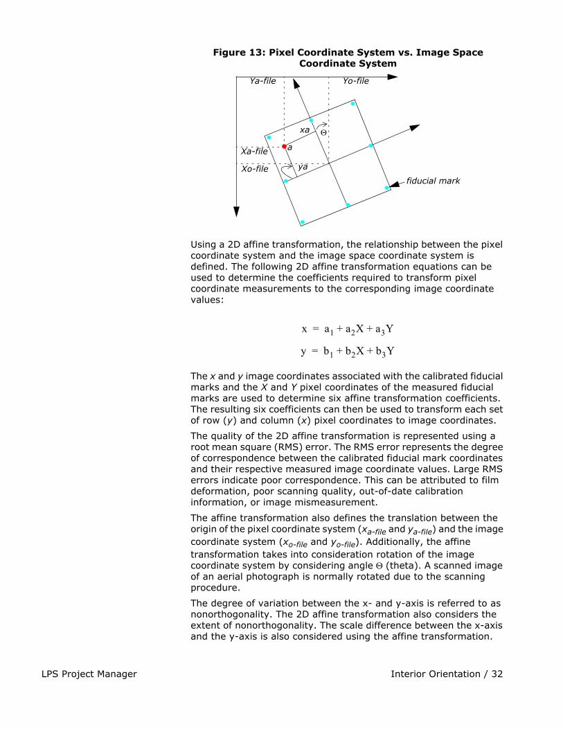
Since the image space coordinate system has not yet been defined for each image, the measured image coordinates of the fiducial marks are referenced to a pixel or file coordinate system. The pixel coordinate system has an x coordinate (column) and a y coordinate (row). The origin of the pixel coordinate system is the upper left corner of the image having a row and column value of 0 and 0, respectively. Figure 13 illustrates the difference between the pixel and image space coordinate system.
Interior Orientation / 32LPS Project Manager
Figure 13: Pixel Coordinate System vs. Image Space Coordinate System
Using a 2D affine transformation, the relationship between the pixel coordinate system and the image space coordinate system is defined. The following 2D affine transformation equations can be used to determine the coefficients required to transform pixel coordinate measurements to the corresponding image coordinate values:
The x and y image coordinates associated with the calibrated fiducial marks and the X and Y pixel coordinates of the measured fiducial marks are used to determine six affine transformation coefficients. The resulting six coefficients can then be used to transform each set of row (y) and column (x) pixel coordinates to image coordinates.
The quality of the 2D affine transformation is represented using a root mean square (RMS) error. The RMS error represents the degree of correspondence between the calibrated fiducial mark coordinates and their respective measured image coordinate values. Large RMS errors indicate poor correspondence. This can be attributed to film deformation, poor scanning quality, out-of-date calibration information, or image mismeasurement.
The affine transformation also defines the translation between the origin of the pixel coordinate system (xa-file and ya-file) and the image coordinate system (xo-file and yo-file). Additionally, the affine transformation takes into consideration rotation of the image coordinate system by considering angle (theta). A scanned image of an aerial photograph is normally rotated due to the scanning procedure.
The degree of variation between the x- and y-axis is referred to as nonorthogonality. The 2D affine transformation also considers the extent of nonorthogonality. The scale difference between the x-axis and the y-axis is also considered using the affine transformation.
fiducial mark
Ya-file Yo-file
Xa-file
Xo-file
xa
ya
a
x a1 a2X a3Y+ +=
y b1 b2X b3Y+ +=
LPS Project Manager Interior Orientation / 33
For more information, see “Fiducial Orientation”.
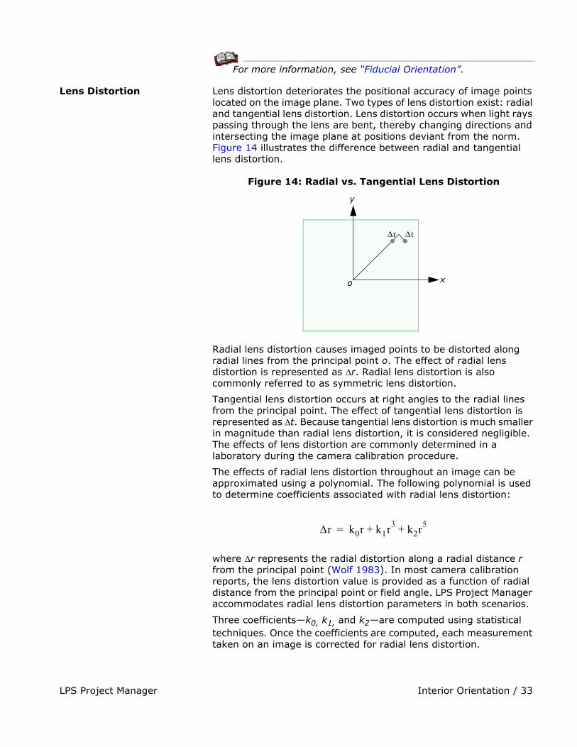
Lens Distortion Lens distortion deteriorates the positional accuracy of image points located on the image plane. Two types of lens distortion exist: radial and tangential lens distortion. Lens distortion occurs when light rays passing through the lens are bent, thereby changing directions and intersecting the image plane at positions deviant from the norm. Figure 14 illustrates the difference between radial and tangential lens distortion.
Figure 14: Radial vs. Tangential Lens Distortion
Radial lens distortion causes imaged points to be distorted along radial lines from the principal point o. The effect of radial lens distortion is represented as r. Radial lens distortion is also commonly referred to as symmetric lens distortion.
Tangential lens distortion occurs at right angles to the radial lines from the principal point. The effect of tangential lens distortion is represented as t. Because tangential lens distortion is much smaller in magnitude than radial lens distortion, it is considered negligible. The effects of lens distortion are commonly determined in a laboratory during the camera calibration procedure.
The effects of radial lens distortion throughout an image can be approximated using a polynomial. The following polynomial is used to determine coefficients associated with radial lens distortion:
where r represents the radial distortion along a radial distance r from the principal point (Wolf 1983). In most camera calibration reports, the lens distortion value is provided as a function of radial distance from the principal point or field angle. LPS Project Manager accommodates radial lens distortion parameters in both scenarios.
Three coefficients—k0, k1, and k2—are computed using statistical techniques. Once the coefficients are computed, each measurement taken on an image is corrected for radial lens distortion.
r t
y
xo
r k0r k1r3 k2r
5+ +=

Exterior Orientation / 34LPS Project Manager
Exterior Orientation
Exterior orientation defines the position and angular orientation of the camera that captured an image. The variables defining the position and orientation of an image are referred to as the elements of exterior orientation. The elements of exterior orientation define the characteristics associated with an image at the time of exposure or capture. The positional elements of exterior orientation include Xo, Yo, and Zo. They define the position of the perspective center (O) with respect to the ground space coordinate system (X, Y, and Z). Zo is commonly referred to as the height of the camera above sea level, which is commonly defined by a datum.
The angular or rotational elements of exterior orientation describe the relationship between the ground space coordinate system (X, Y, and Z) and the image space coordinate system (x, y, and z). Three rotation angles are commonly used to define angular orientation. They are omega (�), phi (�), and kappa (�). Figure 15 illustrates the elements of exterior orientation. Figure 16 illustrates the individual angles (�, �, and �) of exterior orientation.
Figure 15: Elements of Exterior Orientation
X
Y
Z
Xp
Yp
Zp
Xo
Zo
Yo
O
o p
Ground Point P
���
x
yz
x´
y´
z´
yp
xp
f
LPS Project Manager Exterior Orientation / 35
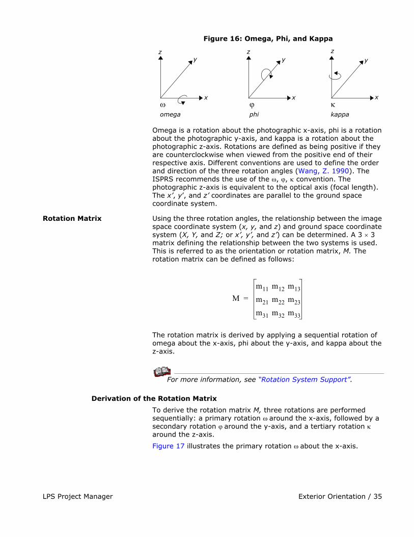
Figure 16: Omega, Phi, and Kappa
Omega is a rotation about the photographic x-axis, phi is a rotation about the photographic y-axis, and kappa is a rotation about the photographic z-axis. Rotations are defined as being positive if they are counterclockwise when viewed from the positive end of their respective axis. Different conventions are used to define the order and direction of the three rotation angles (Wang, Z. 1990). The ISPRS recommends the use of the �, �, � convention. The photographic z-axis is equivalent to the optical axis (focal length). The x’, y’, and z’ coordinates are parallel to the ground space coordinate system.
Rotation Matrix Using the three rotation angles, the relationship between the image space coordinate system (x, y, and z) and ground space coordinate system (X, Y, and Z; or x’, y’, and z’) can be determined. A 3 � 3 matrix defining the relationship between the two systems is used. This is referred to as the orientation or rotation matrix, M. The rotation matrix can be defined as follows:
The rotation matrix is derived by applying a sequential rotation of omega about the x-axis, phi about the y-axis, and kappa about the z-axis.
For more information, see “Rotation System Support”.
Derivation of the Rotation Matrix
To derive the rotation matrix M, three rotations are performed sequentially: a primary rotation ��around the x-axis, followed by a secondary rotation ��around the y-axis, and a tertiary rotation � around the z-axis.
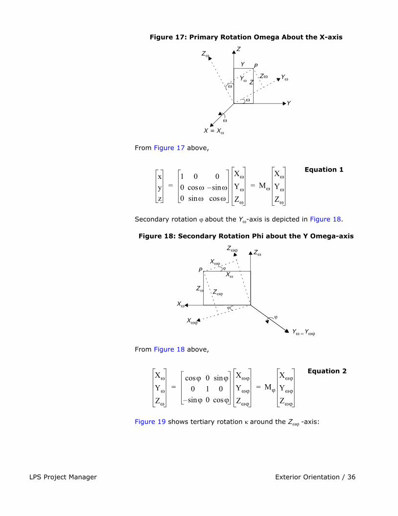
Figure 17 illustrates the primary rotation ��about the x-axis.
� ��
zy
x
omega
zy
x
zy
x
kappaphi
Mm11 m12 m13
m21 m22 m23
m31 m32 m33
=
Exterior Orientation / 36LPS Project Manager
Figure 17: Primary Rotation Omega About the X-axis
From Figure 17 above,
Secondary rotation ��about the Y�-axis is depicted in Figure 18.
Figure 18: Secondary Rotation Phi about the Y Omega-axis
From Figure 18 above,
Figure 19 shows tertiary rotation ��around the Z�� -axis:
Z
Y
X = X�
P
Z�
Y�
Y
Z�Y�
�
Z�
�
xyz
1 0 00 �cos �sin–0 �sin �cos
X�
Y�
Z�
M�
X�
Y�
Z�
= =
Equation 1
Z�Z��
X��
X�P
Z�
X��
X�
Z��
�
�
Y�����Y��
�
X�
Y�
Z�
�cos 0 �sin0 1 0�sin– 0 �cos
X��
Y��
Z��
M�
X��
Y��
Z��
= =
Equation 2

LPS Project Manager Exterior Orientation / 37
Figure 19: Tertiary Rotation Kappa About the Z Omega Phi-axis
From Figure 19 above,
By combining Equation 1, Equation 2, and Equation 3, a relationship can be defined between the coordinates of an object point (P) relative to the (X, Y, Z) and (X��� , Y��� , Z����) coordinate systems:
In Equation 4, replace
with M, which is a 3 ��3 matrix:
where each entry of the matrix can be computed by:
Z�����Z����
Y����
Y���
X����X���
Y����P
�X���X����
Y���
��
��
��
X��
Y��
Z��
�cos �sin– 0�sin �cos 0
0 0 1
X���
Y���
Z���
M�
X���
Y���
Z���
= =
Equation 3
P M� M� M�� P�����= Equation 4
M� M� M���
Mm11 m12 m13
m21 m22 m23
m31 m32 m33
=

Exterior Orientation / 38LPS Project Manager
The Collinearity Equation The following section defines the relationship between the camera/sensor, the image, and the ground. Most photogrammetric tools utilize the following formulas in one form or another.
With reference to Figure 15, an image vector a can be defined as the vector from the exposure station O to the Image Point p. A ground space or object space vector A can be defined as the vector from the exposure station O to the Ground Point P. The image vector and ground vector are collinear, inferring that a line extending from the exposure station to the image point and to the ground is linear.
The image vector and ground vector are only collinear if one is a scalar multiple of the other. Therefore, the following statement can be made:
In this equation, k is a scalar multiple. The image and ground vectors must be within the same coordinate system. Therefore, image vector a is comprised of the following components:
Here, xo and yo represent the image coordinates of the principal point.
Similarly, the ground vector can be formulated as follows:
M11 �cos �cos�=M12 �cos– �sin�=M13 �sin=
M21 �cos �sin� �sin �sin �cos��+=M22 �cos �cos �sin �sin �sin��–�=M23 �sin– �cos�=
M31 �sin �sin �cos �sin �cos��–�=M32 �sin �cos �cos �sin �sin��+�=M33 �cos �cos�=
a kA=
axp xo–yp yo–
f–
=
AXp Xo–Yp Yo–Zp Zo–
=
LPS Project Manager Photogrammetric Solutions / 39
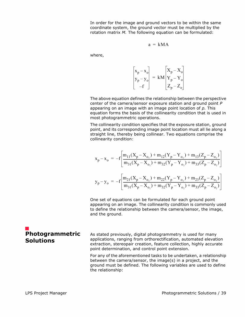
In order for the image and ground vectors to be within the same coordinate system, the ground vector must be multiplied by the rotation matrix M. The following equation can be formulated:
where,
The above equation defines the relationship between the perspective center of the camera/sensor exposure station and ground point P appearing on an image with an image point location of p. This equation forms the basis of the collinearity condition that is used in most photogrammetric operations.
The collinearity condition specifies that the exposure station, ground point, and its corresponding image point location must all lie along a straight line, thereby being collinear. Two equations comprise the collinearity condition:
One set of equations can be formulated for each ground point appearing on an image. The collinearity condition is commonly used to define the relationship between the camera/sensor, the image, and the ground.
Photogrammetric Solutions
As stated previously, digital photogrammetry is used for many applications, ranging from orthorectification, automated elevation extraction, stereopair creation, feature collection, highly accurate point determination, and control point extension.
For any of the aforementioned tasks to be undertaken, a relationship between the camera/sensor, the image(s) in a project, and the ground must be defined. The following variables are used to define the relationship:
a kMA=
xp xo–yp yo–
f–
kMXp Xo–Yp Yo–Zp Zo–
=
xp xo– f–m11 Xp Xo1 �– m12 Yp Yo1 �– m13 Zp Zo1 �–�+�+�
m31 Xp Xo1–� � m32 Yp Yo1–� � m33 Zp Zo1–� �+ +-------------------------------------------------------------------------------------------------------------------------=
yp yo– f–m21 Xp Xo1 �– m22 Yp Yo1 �– m23 Zp Zo1 �–�+�+�
m31 Xp Xo1–� � m32 Yp Yo1–� � m33 Zp Zo1–� �+ +-------------------------------------------------------------------------------------------------------------------------=
Photogrammetric Solutions / 40LPS Project Manager
• exterior orientation parameters for each image
• interior orientation parameters for each image
• accurate representation of the ground
Well-known obstacles in photogrammetry include defining the interior and exterior orientation parameters for each image in a project using a minimum number of GCPs. Due to the time-consuming and labor intensive procedures associated with collecting ground control, most photogrammetric applications do not have an abundant number3 of GCPs. Additionally, the exterior orientation parameters associated with an image are normally unknown.
Depending on the input data provided, photogrammetric techniques such as space resection, space forward intersection, and bundle block adjustment are used to define the variables required to perform orthorectification, automated DEM extraction, stereopair creation, highly accurate point determination, and control point extension.
Space Resection Space resection is a technique that is commonly used to determine the exterior orientation parameters associated with one image or many images based on known GCPs. Space resection uses the collinearity condition. Space resection using the collinearity condition specifies that, for any image, the exposure station, the ground point, and its corresponding image point must lie along a straight line.
If a minimum of three GCPs is known in the X, Y, and Z direction, space resection techniques can be used to determine the six exterior orientation parameters associated with an image. Space resection assumes that camera information is available.
Space resection is commonly used to perform single frame orthorectification, where one image is processed at a time. If multiple images are being used, space resection techniques require that a minimum of three GCPs be located on each image being processed.
Using the collinearity condition, the positions of the exterior orientation parameters are computed. Light rays originating from at least three GCPs intersect through the image plane, through the image positions of the GCPs, and resect at the perspective center of the camera or sensor. Using least squares adjustment techniques, the most probable positions of exterior orientation can be computed. Space resection techniques can be applied to one image or multiple images.
LPS Project Manager Photogrammetric Solutions / 41
Space Forward Intersection
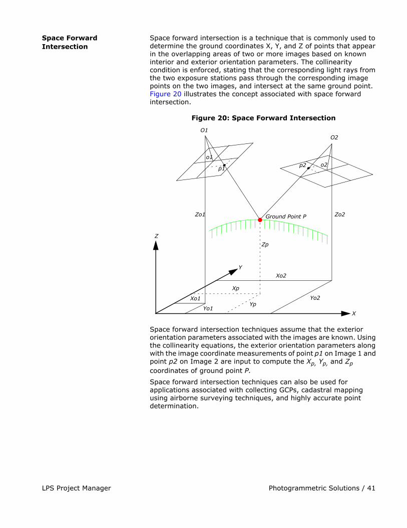
Space forward intersection is a technique that is commonly used to determine the ground coordinates X, Y, and Z of points that appear in the overlapping areas of two or more images based on known interior and exterior orientation parameters. The collinearity condition is enforced, stating that the corresponding light rays from the two exposure stations pass through the corresponding image points on the two images, and intersect at the same ground point. Figure 20 illustrates the concept associated with space forward intersection.
Figure 20: Space Forward Intersection
Space forward intersection techniques assume that the exterior orientation parameters associated with the images are known. Using the collinearity equations, the exterior orientation parameters along with the image coordinate measurements of point p1 on Image 1 and point p2 on Image 2 are input to compute the Xp, Yp, and Zp coordinates of ground point P.
Space forward intersection techniques can also be used for applications associated with collecting GCPs, cadastral mapping using airborne surveying techniques, and highly accurate point determination.
X
Y
Z
Xp
Yp
Zp
Xo1 Yo2
Zo1
Xo2
Yo1
Zo2
O1
o1
O2
o2p1
p2
Ground Point P
Photogrammetric Solutions / 42LPS Project Manager
Bundle Block Adjustment For mapping projects having more than two images, the use of space intersection and space resection techniques is limited. This can be attributed to the lack of information required to perform these tasks. For example, it is fairly uncommon for the exterior orientation parameters to be highly accurate for each photograph or image in a project, since these values are generated photogrammetrically. Airborne GPS and INS techniques normally provide initial approximations to exterior orientation, but the final values for these parameters must be adjusted to attain higher accuracies.
Similarly, rarely are there enough accurate GCPs for a project of 30 or more images to perform space resection (i.e., a minimum of 90 is required). In the case that there are enough GCPs, the time required to identify and measure all of the points would be lengthy.
The costs associated with block triangulation and subsequent orthorectification are largely dependent on the number of GCPs used. To minimize the costs of a mapping project, fewer GCPs are collected and used. To ensure that high accuracies are attained, an approach known as bundle block adjustment is used.
A bundle block adjustment is best defined by examining the individual words in the term. A bundled solution is computed including the exterior orientation parameters of each image in a block and the X, Y, and Z coordinates of tie points and adjusted GCPs. A block of images contained in a project is simultaneously processed in one solution. A statistical technique known as least squares adjustment is used to estimate the bundled solution for the entire block while also minimizing and distributing error.
Block triangulation is the process of defining the mathematical relationship between the images contained within a block, the camera or sensor model, and the ground. Once the relationship has been defined, accurate imagery and geographic information concerning the Earth’s surface can be created.
When processing frame camera, digital camera, videography, and nonmetric camera imagery, block triangulation is commonly referred to as aerial triangulation (AT). When processing imagery collected with a pushbroom sensor, block triangulation is commonly referred to as triangulation.
There are several models for block triangulation. The common models used in photogrammetry are block triangulation with the strip method, the independent model method, and the bundle method. Among them, the bundle block adjustment is the most rigorous of the above methods, considering the minimization and distribution of errors. Bundle block adjustment uses the collinearity condition as the basis for formulating the relationship between image space and ground space. LPS Project Manager uses bundle block adjustment techniques.
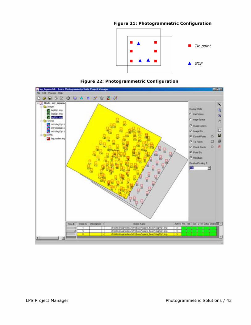
In order to understand the concepts associated with bundle block adjustment, an example comprising two images with three GCPs whose X, Y, and Z coordinates are known is used. Additionally, six tie points are available. Figure 21 illustrates the photogrammetric configuration. Figure 22 illustrates the photogrammetric configuration in the LPS Project Graphic Status window.
LPS Project Manager Photogrammetric Solutions / 43
Figure 21: Photogrammetric Configuration
Figure 22: Photogrammetric Configuration
Tie point
GCP
Photogrammetric Solutions / 44LPS Project Manager
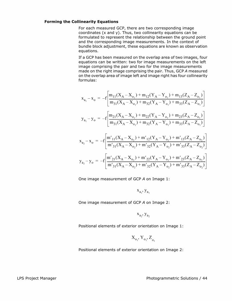
Forming the Collinearity Equations
For each measured GCP, there are two corresponding image coordinates (x and y). Thus, two collinearity equations can be formulated to represent the relationship between the ground point and the corresponding image measurements. In the context of bundle block adjustment, these equations are known as observation equations.
If a GCP has been measured on the overlap area of two images, four equations can be written: two for image measurements on the left image comprising the pair and two for the image measurements made on the right image comprising the pair. Thus, GCP A measured on the overlap area of image left and image right has four collinearity formulas:
One image measurement of GCP A on Image 1:
One image measurement of GCP A on Image 2:
Positional elements of exterior orientation on Image 1:
Positional elements of exterior orientation on Image 2:
xa1 xo– f–m11 XA Xo1 �– m12 YA Yo1 �– m13 ZA Zo1 �–�+�+�
m31 XA Xo1–� � m32 YA Yo1–� � m33 ZA Zo1–� �+ +----------------------------------------------------------------------------------------------------------------------------=
ya1 yo– f–m21 XA Xo1 �– m22 YA Yo1 �– m23 ZA Zo1 �–�+�+�
m31 XA Xo1–� � m32 YA Yo1–� � m33 ZA Zo1–� �+ +----------------------------------------------------------------------------------------------------------------------------=
xa2 xo– f–m 11 XA Xo2 �– m 12 YA Yo2 �– m 13 ZA Zo2 �–�+�+�
m 31 XA Xo2–� � m 32 YA Yo2–� � m 33 ZA Zo2–� �+ +----------------------------------------------------------------------------------------------------------------------------------=
ya2 yo– f–m 21 XA Xo2 �– m 22 YA Yo2 �– m 23 ZA Zo2 �–�+�+�
m 31 XA Xo2–� � m 32 YA Yo2–� � m 33 ZA Zo2–� �+ +----------------------------------------------------------------------------------------------------------------------------------=
xa1 ya1�
xa2 ya2�
Xo1 Yo1 Z� o1�
LPS Project Manager Photogrammetric Solutions / 45
If three GCPs have been measured on the overlap area of two images, twelve equations can be formulated (four equations for each GCP).
Additionally, if six tie points have been measured on the overlap areas of the two images, twenty-four equations can be formulated (four for each tie point). This is a total of 36 observation equations.
The previous scenario has the following unknowns:
• six exterior orientation parameters for the left image (that is, X, Y, Z, omega, phi, kappa)
• six exterior orientation parameters for the right image (that is, X, Y, Z, omega, phi, kappa)
• X, Y, and Z coordinates of the tie points. Thus, for six tie points, this includes eighteen unknowns (six tie points times three X, Y, Z coordinates)
The total number of unknowns is 30. The overall quality of a bundle block adjustment is largely a function of the quality and redundancy in the input data. In this scenario, the redundancy in the project can be computed by subtracting the number of unknowns, 30, from the number of knowns, 36. The resulting redundancy is six. This term is commonly referred to as the degrees of freedom in a solution.
Once each observation equation is formulated, the collinearity condition can be solved using an approach referred to as least squares adjustment.
Least Squares Adjustment
Least squares adjustment is a statistical technique that is used to estimate the unknown parameters associated with a solution while also minimizing error within the solution. With respect to block triangulation, least squares adjustment techniques are used to:
• estimate or adjust the values associated with exterior orientation
• estimate the X, Y, and Z coordinates associated with tie points
• estimate or adjust the values associated with interior orientation
• minimize and distribute data error through the network of observations
Data error is attributed to the inaccuracy associated with the input GCP coordinates, measured tie point and GCP image positions, camera information, and systematic errors.
The least squares approach requires iterative processing until a solution is attained. A solution is obtained when the residuals, or errors, associated with the input data are minimized.
Xo2 Yo2 Z� o2�

Photogrammetric Solutions / 46LPS Project Manager
The least squares approach involves determining the corrections to the unknown parameters based on the criteria of minimizing input measurement residuals. The residuals are derived from the difference between the measured (i.e., user input) and computed value for any particular measurement in a project. In the block triangulation process, a functional model can be formed based upon the collinearity equations.
The functional model refers to the specification of an equation that can be used to relate measurements to parameters. In the context of photogrammetry, measurements include the image locations of GCPs and GCP coordinates, while the exterior orientations of all the images are important parameters estimated by the block triangulation process.
The residuals, which are minimized, include the image coordinates of the GCPs and tie points along with the known ground coordinates of the GCPs. A simplified version of the least squares condition can be broken down into a formula that includes a weight matrix P, as follows:
In this equation,
V = the matrix containing the image coordinate residualsA = the matrix containing the partial derivatives with
respect to the unknown parameters, including exterior orientation, interior orientation, XYZ tie point, and GCP coordinates
X = the matrix containing the corrections to the unknown parameters
L = the matrix containing the input observations (i.e., image coordinates and GCP coordinates)
The components of the least squares condition are directly related to the functional model based on collinearity equations. The A matrix is formed by differentiating the functional model, which is based on collinearity equations, with respect to the unknown parameters such as exterior orientation, etc. The L matrix is formed by subtracting the initial results obtained from the functional model with newly estimated results determined from a new iteration of processing. The X matrix contains the corrections to the unknown exterior orientation parameters. The X matrix is calculated in the following manner:
In this equation,
X = the matrix containing the corrections to the unknown parameters t
V AX L–=
X AtPA ��1–AtPL=

LPS Project Manager Photogrammetric Solutions / 47
A = the matrix containing the partial derivatives with respect to the unknown parameters
t = the matrix transposedP = the matrix containing the weights of the observationsL = the matrix containing the observations
Once a least squares iteration of processing is completed, the corrections to the unknown parameters are added to the initial estimates. For example, if initial approximations to exterior orientation are provided from airborne GPS and INS information, the estimated corrections computed from the least squares adjustment are added to the initial value to compute the updated exterior orientation values. This iterative process of least squares adjustment continues until the corrections to the unknown parameters are less than a user-specified threshold (commonly referred to as a convergence value).
The V residual matrix is computed at the end of each iteration of processing. Once an iteration is complete, the new estimates for the unknown parameters are used to recompute the input observations such as the image coordinate values. The difference between the initial measurements and the new estimates is obtained to provide the residuals. Residuals provide preliminary indications of the accuracy of a solution. The residual values indicate the degree to which a particular observation (input) fits with the functional model. For example, the image residuals have the capability of reflecting GCP collection in the field. After each successive iteration of processing, the residuals become smaller until they are satisfactorily minimized.
Once the least squares adjustment is completed, the block triangulation results include:
• final exterior orientation parameters of each image in a block and their accuracy
• final interior orientation parameters of each image in a block and their accuracy
• X, Y, and Z tie point coordinates and their accuracy
• adjusted GCP coordinates and their residuals
• image coordinate residuals
The results from the block triangulation are then used as the primary input for the following tasks:
• stereopair creation
• feature collection
• highly accurate point determination
Photogrammetric Solutions / 48LPS Project Manager
• DEM extraction
• orthorectification
Self-calibrating Bundle Adjustment
Normally, there are more or less systematic errors related to the imaging and processing system, such as lens distortion, film distortion, atmosphere refraction, scanner errors, and so on. These errors reduce the accuracy of triangulation results, especially in dealing with large-scale imagery and high accuracy triangulation. There are several ways to reduce the influences of the systematic errors, like a posteriori compensation, test-field calibration, and the most common approach—self-calibration (Konecny 1994; Wang, Z. 1990).
The self-calibrating methods use additional parameters in the triangulation process to eliminate the systematic errors. How well it works depends on many factors such as the strength of the block (overlap amount, crossing flight lines), the GCP and tie point distribution and amount, the size of systematic errors versus random errors, the significance of the additional parameters, the correlation between additional parameters, and other unknowns.
There was intensive research and development for additional parameter models in photogrammetry in the ‘70s and the ‘80s, and many research results are available (e.g., Bauer and Müller 1972; Ebner 1976; Grün 1978; Jacobsen 1980 and Jacobsen 1982; Li 1985; Wang, Y. 1988; and Stojic, Chandler, Ashmore, and Luce 1998). Based on these scientific reports, LPS Project Manager provides four groups of additional parameters for you to choose in different triangulation circumstances. In addition, LPS Project Manager allows the interior orientation parameters to be analytically calibrated with its self-calibrating bundle block adjustment.
Automatic Gross Error Detection
Normal random errors are subject to statistical normal distribution. In contrast, gross errors refer to errors that are large and are not subject to normal distribution. The gross errors among the input data for triangulation can lead to unreliable results. Research during the 80s in the photogrammetric community resulted in significant achievements in automatic gross error detection in the triangulation process (e.g., Kubik 1982; Li 1983 and Li 1985; Jacobsen 1984; El-Hakim and Ziemann 1984; Wang, Y. 1988).
Methods for gross error detection began with residual checking using data-snooping and were later extended to robust estimation (Wang, Z. 1990). The most common robust estimation method is the iteration with selective weight functions. Based on the scientific research results from the photogrammetric community, LPS Project Manager offers two robust error detection methods within the triangulation process.
For more information, see “Automated Gross Error Checking”.
LPS Project Manager GCPs / 49
The effect of the automatic error detection depends not only on the mathematical model, but also depends on the redundancy in the block. Therefore, more tie points in more overlap areas contribute better gross error detection. In addition, inaccurate GCPs can distribute their errors to correct tie points; therefore, the ground and image coordinates of GCPs should have better accuracy than tie points when comparing them within the same scale space.
GCPs The instrumental component of establishing an accurate relationship between the images in a project, the camera/sensor, and the ground is GCPs. GCPs are identifiable features located on the Earth’s surface whose ground coordinates in X, Y, and Z are known. A full GCP has associated with it X, Y, and Z (elevation of the point) coordinates. A horizontal GCP only specifies the X, Y coordinates, while a vertical GCP only specifies the Z coordinate.
The following features on the Earth’s surface are commonly used as GCPs:
• intersection of roads
• utility infrastructure (e.g., fire hydrants and manhole covers)
• intersection of agricultural plots of land
• survey benchmarks
Depending on the type of mapping project, GCPs can be collected from the following sources:
• theodolite survey (millimeter to centimeter accuracy)
• total station survey (millimeter to centimeter accuracy)
• ground GPS (centimeter to meter accuracy)
• planimetric and topographic maps (accuracy varies as a function of map scale, approximate accuracy between several meters to 40 meters or more)
• digital orthorectified images (X and Y coordinates can be collected to an accuracy dependent on the resolution of the orthorectified image)
• DEMs (for the collection of vertical GCPs having Z coordinates associated with them, where accuracy is dependent on the resolution of the DEM and the accuracy of the input DEM)
GCPs / 50LPS Project Manager
When imagery or photography is exposed, GCPs are recorded and subsequently displayed on the photograph or image. During GCP measurement in LPS Project Manager, the image positions of GCPs appearing on an image, or on the overlap area of the images, are collected.
It is highly recommended that a greater number of GCPs be available than are actually used in the block triangulation. Additional GCPs can be used as check points to independently verify the overall quality and accuracy of the block triangulation solution. A check point analysis compares the photogrammetrically computed ground coordinates of the check points to the original values. The result of the analysis is an RMSE that defines the degree of correspondence between the computed values and the original values. Lower RMSE values indicate better results.
GCP Requirements The minimum GCP requirements for an accurate mapping project vary with respect to the size of the project. With respect to establishing a relationship between image space and ground space, the theoretical minimum number of GCPs is two GCPs having X, Y, and Z coordinates (six observations) and one GCP having a Z coordinate (one observation). This is a total of seven observations.
In establishing the mathematical relationship between image space and object space, seven parameters defining the relationship must be determined. The seven parameters include a scale factor (describing the scale difference between image space and ground space); X, Y, and Z (defining the positional differences between image space and object space); and three rotation angles (omega, phi, and kappa) defining the rotational relationship between image space and ground space.
In order to compute a unique solution, at least seven known parameters must be available. In using the two XYZ GCPs and one vertical (Z) GCP, the relationship can be defined. However, to increase the accuracy of a mapping project, using more GCPs is highly recommended.
The following descriptions are provided for various projects:
Processing One Image
When processing one image for the purpose of orthorectification (that is, a single frame orthorectification), the minimum number of GCPs required is three. Each GCP must have an X, Y, and Z coordinate associated with it. The GCPs should be evenly distributed to ensure that the camera/sensor is accurately modeled.
Processing a Strip of Images
When processing a strip of adjacent images, two GCPs for every third image are recommended. To increase the quality of orthorectification, measuring three GCPs at the corner edges of a strip is advantageous. Thus, during block triangulation a stronger geometry can be enforced in areas where there is less redundancy such as the corner edges of a strip or a block.

LPS Project Manager GCPs / 51
Figure 23 illustrates the GCP configuration for a strip of images having 60% overlap. The triangles represent the GCPs. Thus, the image positions of the GCPs are measured on the overlap areas of the imagery.
Figure 23: GCP Configuration
Processing Multiple Strips of Imagery
Figure 24 depicts the standard GCP configuration for a block of images, comprising four strips of images, each containing eight overlapping images.
Figure 24: GCPs in a Block of Images
In this case, the GCPs form a strong geometric network of observations. As a general rule, it is advantageous to have at least one GCP on every third image of a block. Additionally, whenever possible, locate GCPs that lie on multiple images, around the outside edges of a block and at certain distances from one another within the block.
Tie Points / 52LPS Project Manager
Tie Points A tie point is a point whose ground coordinates are not known, but is visually recognizable in the overlap area between two or more images. The corresponding image positions of tie points appearing on the overlap areas of multiple images is identified and measured. Ground coordinates for tie points are computed during block triangulation. Tie points can be measured both manually and automatically.
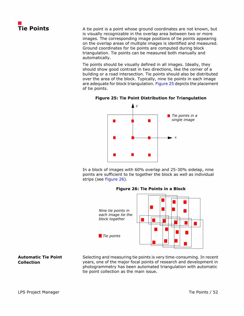
Tie points should be visually defined in all images. Ideally, they should show good contrast in two directions, like the corner of a building or a road intersection. Tie points should also be distributed over the area of the block. Typically, nine tie points in each image are adequate for block triangulation. Figure 25 depicts the placement of tie points.
Figure 25: Tie Point Distribution for Triangulation
In a block of images with 60% overlap and 25-30% sidelap, nine points are sufficient to tie together the block as well as individual strips (see Figure 26).
Figure 26: Tie Points in a Block
Automatic Tie Point Collection
Selecting and measuring tie points is very time-consuming. In recent years, one of the major focal points of research and development in photogrammetry has been automated triangulation with automatic tie point collection as the main issue.
Tie points in asingle image
y
x
Nine tie points ineach image tie theblock together
Tie points

LPS Project Manager Image Matching Techniques / 53
Another issue of automated triangulation is the automatic control point identification, which is still unsolved due to the complexity of the scenario. There are several valuable research results detailing automated triangulation (e.g., Agouris and Schenk 1996; Heipke 1996; Krzystek 1998; Mayr 1995; Schenk 1997; Tang, Braun, and Debitsch 1997; Tsingas 1995; Wang, Y. 1998).
After investigating the advantages and the weaknesses of the existing methods, LPS Project Manager was designed to incorporate an advanced method for automatic tie point collection. It is designed to work with a variety of digital images such as aerial images, satellite images, digital camera images, and close-range images. It also supports the processing of multiple strips including adjacent, diagonal, and cross-strips.
Automatic tie point collection within LPS Project Manager successfully performs the following tasks:
• Automatic block configuration. Based on the initial input requirements, LPS Project Manager automatically detects the relationship of the block with respect to image adjacency.
• Automatic tie point extraction. The feature point extraction algorithms are used here to extract the candidates of tie points.
• Point transfer. Feature points appearing on multiple images are automatically matched and identified.
• Gross error detection. Erroneous points are automatically identified and removed from the solution.
• Tie point selection. The intended number of tie points defined by the user is automatically selected as the final number of tie points.
The image matching strategies incorporated in LPS Project Manager for automatic tie point collection include the coarse-to-fine matching; feature-based matching with geometrical and topological constraints, which is simplified from the structural matching algorithm (Wang, Y. 1998); and the least square matching for the high accuracy of tie points.
Image Matching Techniques
Image matching refers to the automatic identification and measurement of corresponding image points that are located on the overlapping areas of multiple images. The various image matching methods can be divided into three categories including:
• area-based matching
• feature-based matching
• relation-based matching
Image Matching Techniques / 54LPS Project Manager
Area-based Matching Area-based matching is also called signal based matching. This method determines the correspondence between two image areas according to the similarity of their gray level values. The cross-correlation and least squares correlation techniques are well-known methods for area-based matching.
Correlation Windows
Area-based matching uses correlation windows. These windows consist of a local neighborhood of pixels. One example of correlation windows is square neighborhoods (for example, 3 � 3, 5 � 5, 7 � 7 pixels). In practice, the windows vary in shape and dimension based on the matching technique. Area correlation uses the characteristics of these windows to match ground feature locations in one image to ground features on the other.
A reference window is the source window on the first image, which remains at a constant location. Its dimensions are usually square in size (for example, 3 � 3, 5 � 5, and so on). Search windows are candidate windows on the second image that are evaluated relative to the reference window. During correlation, many different search windows are examined until a location is found that best matches the reference window.
Correlation Calculations
Two correlation calculations are described in the following sections: cross-correlation and least squares correlation. Most area-based matching calculations, including these methods, normalize the correlation windows. Therefore, it is not necessary to balance the contrast or brightness prior to running correlation. Cross-correlation is more robust in that it requires a less accurate a priori position than least squares. However, its precision is limited to one pixel. Least squares correlation can achieve precision levels of one-tenth of a pixel, but requires an a priori position that is accurate to about two pixels. In practice, cross-correlation is often followed by least squares for high accuracy.
Cross-correlation
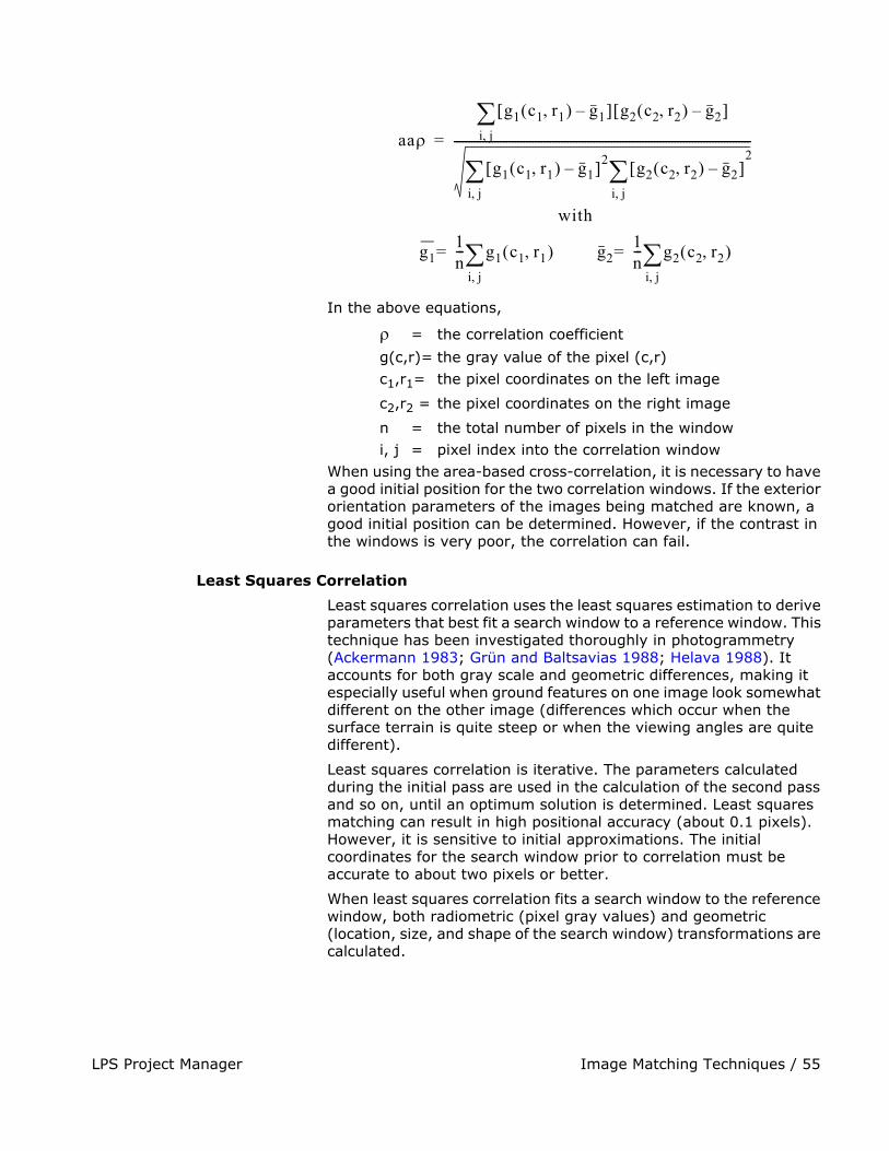
Cross-correlation computes the correlation coefficient of the gray values between the template window and the search window according to the following equation:
LPS Project Manager Image Matching Techniques / 55
In the above equations,
� = the correlation coefficient
g(c,r)= the gray value of the pixel (c,r) c1,r1= the pixel coordinates on the left image
c2,r2 = the pixel coordinates on the right image
n = the total number of pixels in the windowi, j = pixel index into the correlation window
When using the area-based cross-correlation, it is necessary to have a good initial position for the two correlation windows. If the exterior orientation parameters of the images being matched are known, a good initial position can be determined. However, if the contrast in the windows is very poor, the correlation can fail.
Least Squares Correlation
Least squares correlation uses the least squares estimation to derive parameters that best fit a search window to a reference window. This technique has been investigated thoroughly in photogrammetry (Ackermann 1983; Grün and Baltsavias 1988; Helava 1988). It accounts for both gray scale and geometric differences, making it especially useful when ground features on one image look somewhat different on the other image (differences which occur when the surface terrain is quite steep or when the viewing angles are quite different).
Least squares correlation is iterative. The parameters calculated during the initial pass are used in the calculation of the second pass and so on, until an optimum solution is determined. Least squares matching can result in high positional accuracy (about 0.1 pixels). However, it is sensitive to initial approximations. The initial coordinates for the search window prior to correlation must be accurate to about two pixels or better.
When least squares correlation fits a search window to the reference window, both radiometric (pixel gray values) and geometric (location, size, and shape of the search window) transformations are calculated.
aa�
g1 c1 r1�� � g1–� � g2 c2 r2�� � g2–� �i j��
g1 c1 r1�� � g1–� �2 g2 c2 r2�� � g2–� �i j��
2
i j��
------------------------------------------------------------------------------------------------------=
with
g11n--- g1 c1 r1�� �i j��= g2
1n--- g2 c2 r2�� �i j��=

Image Matching Techniques / 56LPS Project Manager
For example, suppose the change in gray values between two correlation windows is represented as a linear relationship. Also assume that the change in the window’s geometry is represented by an affine transformation.
In the equations,
c1,r1 = the pixel coordinate in the reference window
c2,r2 = the pixel coordinate in the search window
g1(c1,r1) = the gray value of pixel (c1,r1)
g2(c2,r2) = the gray value of pixel (c2,r2)
h0, h1 = linear gray value transformation parameters
a0, a1, a2 = affine geometric transformation parameters
b0, b1, b2 = affine geometric transformation parameters
Based on this assumption, the error equation for each pixel is derived, as shown in the following equation:
The values gc and gr are the gradients of g2 (c2,r2).
Feature-based Matching Feature-based matching determines the correspondence between two image features. Most feature-based techniques match extracted point features (this is called feature point matching), as opposed to other features, such as lines or complex objects. The feature points are also commonly referred to as interest points. Poor contrast areas can be avoided with feature-based matching.
In order to implement feature-based matching, the image features must initially be extracted. There are several well-known operators for feature point extraction. Examples include the Moravec Operator, the Dreschler Operator, and the Förstner Operator (Förstner and Gülch 1987; Lü 1988).
After the features are extracted, the attributes of the features are compared between two images. The feature pair having the attributes with the best fit is recognized as a match. LPS Project Manager utilizes the Förstner interest operator to extract feature points.
g2 c2 r2�� � h0 h1g1 c1 r1�� �+=
c2 a0 a1c1 a2r1+ +=
r2 b0 b1c1 b2r1+ +=
v a1 a2c1 a3r1+ +� �gc b1 b2c1 b3r1+ +� �gr h1– h2g1 c1 r1�� �– g+ +=
with g g2 c2 r2�� � g1 c1 r1�� �–=
LPS Project Manager Image Matching Techniques / 57
Relation-based Matching Relation-based matching is also called structural matching (Vosselman and Haala 1992; Wang, Y. 1994 and Wang, Y. 1995). This kind of matching technique uses the image features and the relationship between the features. With relation-based matching, the corresponding image structures can be recognized automatically, without any a priori information. However, the process is time-consuming since it deals with varying types of information. Relation-based matching can also be applied for the automatic recognition of control points.
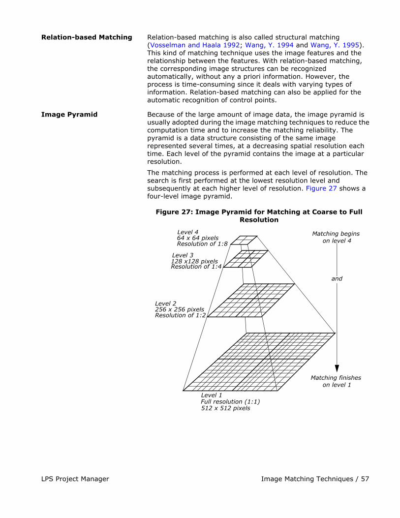
Image Pyramid Because of the large amount of image data, the image pyramid is usually adopted during the image matching techniques to reduce the computation time and to increase the matching reliability. The pyramid is a data structure consisting of the same image represented several times, at a decreasing spatial resolution each time. Each level of the pyramid contains the image at a particular resolution.
The matching process is performed at each level of resolution. The search is first performed at the lowest resolution level and subsequently at each higher level of resolution. Figure 27 shows a four-level image pyramid.
Figure 27: Image Pyramid for Matching at Coarse to Full Resolution
Level 2
Full resolution (1:1)
256 x 256 pixels
Level 1
512 x 512 pixels
Level 3128 x128 pixels
Level 464 x 64 pixels
Matching begins
and
Matching finishes
Resolution of 1:8
Resolution of 1:4
Resolution of 1:2
on level 1
on level 4
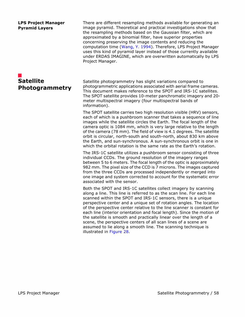
Satellite Photogrammetry / 58LPS Project Manager
LPS Project Manager Pyramid Layers
There are different resampling methods available for generating an image pyramid. Theoretical and practical investigations show that the resampling methods based on the Gaussian filter, which are approximated by a binomial filter, have superior properties concerning preserving the image contents and reducing the computation time (Wang, Y. 1994). Therefore, LPS Project Manager uses this kind of pyramid layer instead of those currently available under ERDAS IMAGINE, which are overwritten automatically by LPS Project Manager.
Satellite Photogrammetry
Satellite photogrammetry has slight variations compared to photogrammetric applications associated with aerial frame cameras. This document makes reference to the SPOT and IRS-1C satellites. The SPOT satellite provides 10-meter panchromatic imagery and 20-meter multispectral imagery (four multispectral bands of information).
The SPOT satellite carries two high resolution visible (HRV) sensors, each of which is a pushbroom scanner that takes a sequence of line images while the satellite circles the Earth. The focal length of the camera optic is 1084 mm, which is very large relative to the length of the camera (78 mm). The field of view is 4.1 degrees. The satellite orbit is circular, north-south and south-north, about 830 km above the Earth, and sun-synchronous. A sun-synchronous orbit is one in which the orbital rotation is the same rate as the Earth’s rotation.
The IRS-1C satellite utilizes a pushbroom sensor consisting of three individual CCDs. The ground resolution of the imagery ranges between 5 to 6 meters. The focal length of the optic is approximately 982 mm. The pixel size of the CCD is 7 microns. The images captured from the three CCDs are processed independently or merged into one image and system corrected to account for the systematic error associated with the sensor.
Both the SPOT and IRS-1C satellites collect imagery by scanning along a line. This line is referred to as the scan line. For each line scanned within the SPOT and IRS-1C sensors, there is a unique perspective center and a unique set of rotation angles. The location of the perspective center relative to the line scanner is constant for each line (interior orientation and focal length). Since the motion of the satellite is smooth and practically linear over the length of a scene, the perspective centers of all scan lines of a scene are assumed to lie along a smooth line. The scanning technique is illustrated in Figure 28.
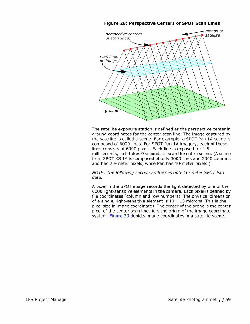
LPS Project Manager Satellite Photogrammetry / 59
Figure 28: Perspective Centers of SPOT Scan Lines
The satellite exposure station is defined as the perspective center in ground coordinates for the center scan line. The image captured by the satellite is called a scene. For example, a SPOT Pan 1A scene is composed of 6000 lines. For SPOT Pan 1A imagery, each of these lines consists of 6000 pixels. Each line is exposed for 1.5 milliseconds, so it takes 9 seconds to scan the entire scene. (A scene from SPOT XS 1A is composed of only 3000 lines and 3000 columns and has 20-meter pixels, while Pan has 10-meter pixels.)
NOTE: The following section addresses only 10-meter SPOT Pan data.
A pixel in the SPOT image records the light detected by one of the 6000 light-sensitive elements in the camera. Each pixel is defined by file coordinates (column and row numbers). The physical dimension of a single, light-sensitive element is 13 � 13 microns. This is the pixel size in image coordinates. The center of the scene is the center pixel of the center scan line. It is the origin of the image coordinate system. Figure 29 depicts image coordinates in a satellite scene.
perspective centers motion of
scan lineson image
ground
satelliteof scan lines
Satellite Photogrammetry / 60LPS Project Manager
Figure 29: Image Coordinates in a Satellite Scene
where,
A = origin of file coordinatesA-XF, A-YF=file coordinate axes
C = origin of image coordinates (center of scene)C-x, C-y=image coordinate axes
SPOT Interior Orientation Figure 30 shows the interior orientation of a satellite scene. The transformation between file coordinates and image coordinates is constant.
y
x
A XF
YF
C6000 lines
6000 pixels
(rows)
(columns)
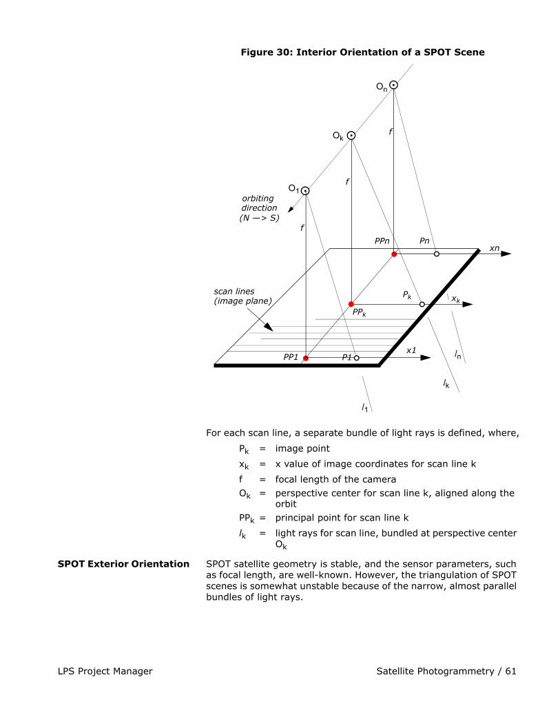
LPS Project Manager Satellite Photogrammetry / 61
Figure 30: Interior Orientation of a SPOT Scene
For each scan line, a separate bundle of light rays is defined, where,
Pk = image point
xk = x value of image coordinates for scan line k
f = focal length of the cameraOk = perspective center for scan line k, aligned along the
orbit PPk = principal point for scan line k
lk = light rays for scan line, bundled at perspective center Ok
SPOT Exterior Orientation SPOT satellite geometry is stable, and the sensor parameters, such as focal length, are well-known. However, the triangulation of SPOT scenes is somewhat unstable because of the narrow, almost parallel bundles of light rays.
P1
xk
O1
Ok
On
PPn
PP1
Pk
Pnxn
x1
f
f
f
l1
lk
lnP1
PPk
orbiting
scan lines(image plane)
direction(N —> S)
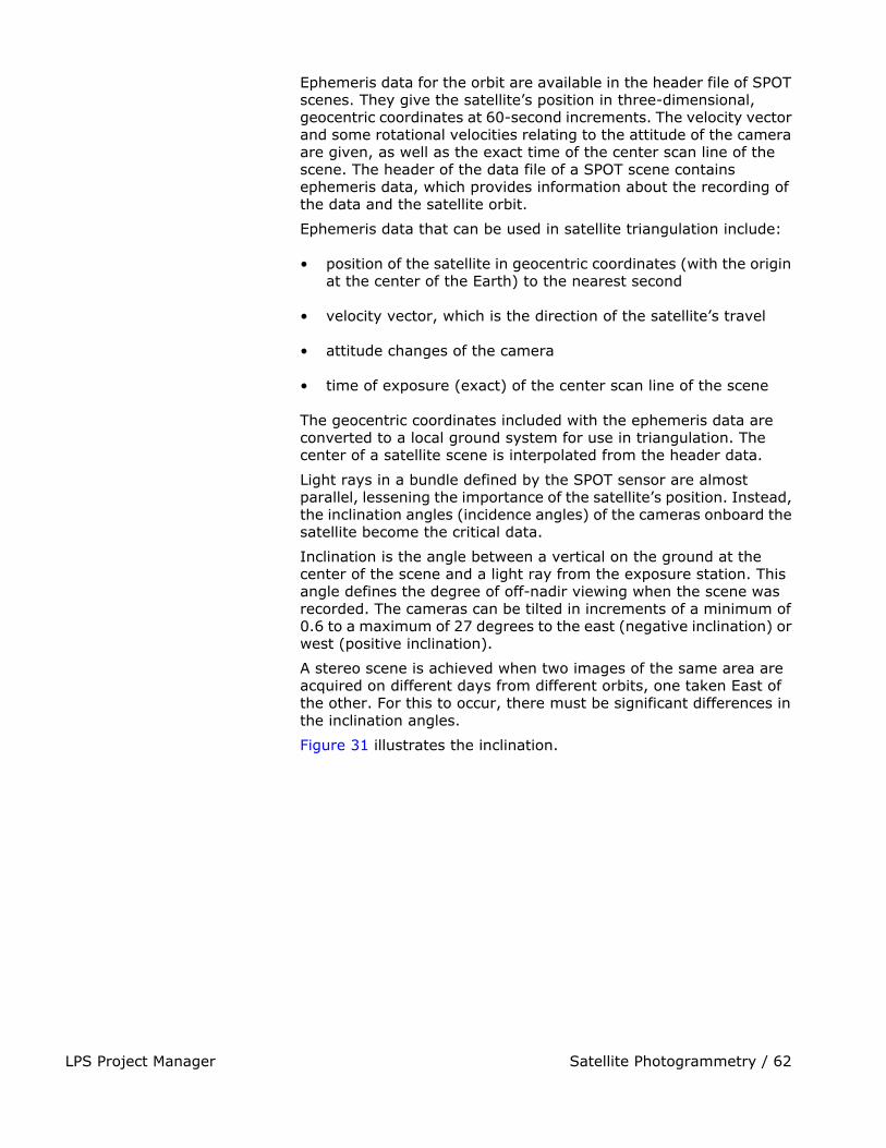
Satellite Photogrammetry / 62LPS Project Manager
Ephemeris data for the orbit are available in the header file of SPOT scenes. They give the satellite’s position in three-dimensional, geocentric coordinates at 60-second increments. The velocity vector and some rotational velocities relating to the attitude of the camera are given, as well as the exact time of the center scan line of the scene. The header of the data file of a SPOT scene contains ephemeris data, which provides information about the recording of the data and the satellite orbit.
Ephemeris data that can be used in satellite triangulation include:
• position of the satellite in geocentric coordinates (with the origin at the center of the Earth) to the nearest second
• velocity vector, which is the direction of the satellite’s travel
• attitude changes of the camera
• time of exposure (exact) of the center scan line of the scene
The geocentric coordinates included with the ephemeris data are converted to a local ground system for use in triangulation. The center of a satellite scene is interpolated from the header data.
Light rays in a bundle defined by the SPOT sensor are almost parallel, lessening the importance of the satellite’s position. Instead, the inclination angles (incidence angles) of the cameras onboard the satellite become the critical data.
Inclination is the angle between a vertical on the ground at the center of the scene and a light ray from the exposure station. This angle defines the degree of off-nadir viewing when the scene was recorded. The cameras can be tilted in increments of a minimum of 0.6 to a maximum of 27 degrees to the east (negative inclination) or west (positive inclination).
A stereo scene is achieved when two images of the same area are acquired on different days from different orbits, one taken East of the other. For this to occur, there must be significant differences in the inclination angles.
Figure 31 illustrates the inclination.

LPS Project Manager Satellite Photogrammetry / 63
Figure 31: Inclination of a Satellite Stereo Scene (View from North to South)
In Figure 31,
C = center of the sceneI- = eastward inclination I+ = westward inclination O1,O2= exposure stations (perspective centers of imagery)
The orientation angle of a satellite scene is the angle between a perpendicular to the center scan line and the North direction. The spatial motion of the satellite is described by the velocity vector. The real motion of the satellite above the ground is further distorted by the Earth’s rotation.
The scanner can produce a nadir view. Nadir is the point directly below the camera. SPOT has off-nadir viewing capability. Off-nadir refers to any point that is not directly beneath the satellite, but is off to an angle (that is, East or West of the nadir), as shown in Figure 32.
C Earth’s surface
orbit 2orbit 1
I -
I +
EAST WEST
sensors
O1 O2
scene coverage
vertical
(ellipsoid)
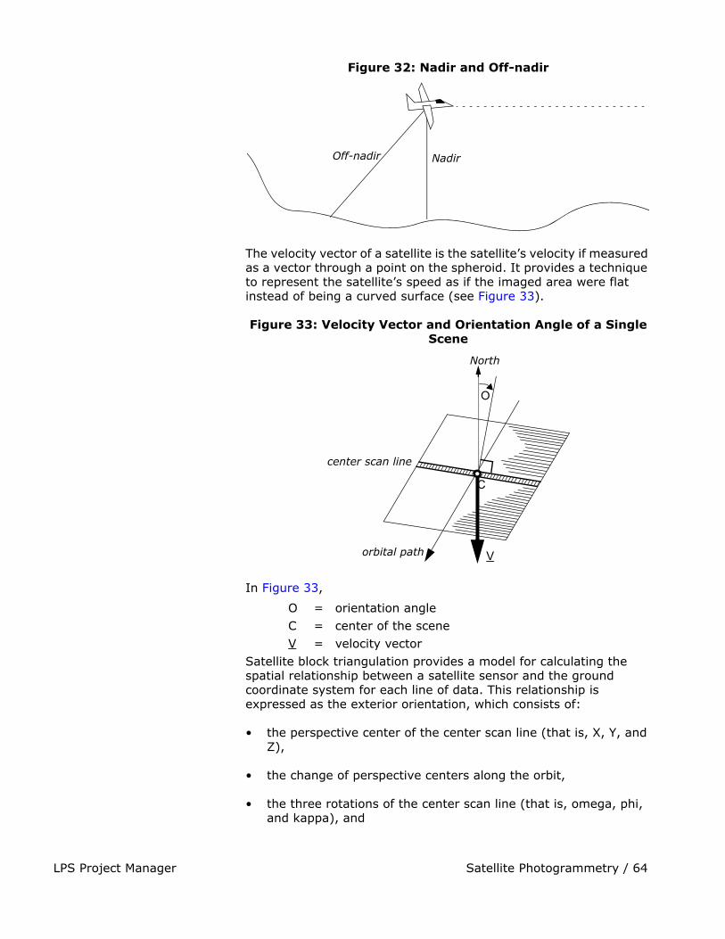
Satellite Photogrammetry / 64LPS Project Manager
Figure 32: Nadir and Off-nadir
The velocity vector of a satellite is the satellite’s velocity if measured as a vector through a point on the spheroid. It provides a technique to represent the satellite’s speed as if the imaged area were flat instead of being a curved surface (see Figure 33).
Figure 33: Velocity Vector and Orientation Angle of a Single Scene
In Figure 33,
O = orientation angleC = center of the sceneV = velocity vector
Satellite block triangulation provides a model for calculating the spatial relationship between a satellite sensor and the ground coordinate system for each line of data. This relationship is expressed as the exterior orientation, which consists of:
• the perspective center of the center scan line (that is, X, Y, and Z),
• the change of perspective centers along the orbit,
• the three rotations of the center scan line (that is, omega, phi, and kappa), and
Off-nadir Nadir
center scan line
orbital path V
C
O
North

LPS Project Manager Satellite Photogrammetry / 65
• the changes of angles along the orbit.
In addition to fitting the bundle of light rays to the known points, satellite block triangulation also accounts for the motion of the satellite by determining the relationship of the perspective centers and rotation angles of the scan lines. It is assumed that the satellite travels in a smooth motion as a scene is being scanned. Therefore, once the exterior orientation of the center scan line is determined, the exterior orientation of any other scan line is calculated based on the distance of that scan line from the center and the changes of the perspective center location and rotation angles.
Bundle adjustment for triangulating a satellite scene is similar to the bundle adjustment used for aerial images. A least squares adjustment is used to derive a set of parameters that comes the closest to fitting the control points to their known ground coordinates, and to intersecting tie points.
The resulting parameters of satellite bundle adjustment are:
• ground coordinates of the perspective center of the center scan line
• rotation angles for the center scan line
• coefficients, from which the perspective center and rotation angles of all other scan lines are calculated
• ground coordinates of all tie points
Collinearity Equations and Satellite Block Triangulation
Modified collinearity equations are used to compute the exterior orientation parameters associated with the respective scan lines in the satellite scenes. Each scan line has a unique perspective center and individual rotation angles. When the satellite moves from one scan line to the next, these parameters change. Due to the smooth motion of the satellite in orbit, the changes are small and can be modeled by low-order polynomial functions.
Control for Satellite Block Triangulation
Both GCPs and tie points can be used for satellite block triangulation of a stereo scene. For triangulating a single scene, only GCPs are used. In this case, space resection techniques are used to compute the exterior orientation parameters associated with the satellite as they existed at the time of image capture. A minimum of six GCPs is necessary. Ten or more GCPs are recommended to obtain a good triangulation result.
The best locations for GCPs in the scene are shown in Figure 34.

Orthorectification / 66LPS Project Manager
Figure 34: Ideal Point Distribution Over a Satellite Scene for Triangulation
Orthorectification Orthorectification is the process of reducing geometric errors inherent within photography and imagery. The variables contributing to geometric errors include, but are not limited to:
• camera and sensor orientation
• systematic error associated with the camera or sensor
• topographic relief displacement
• Earth curvature
By performing block triangulation or single frame resection, the parameters associated with camera and sensor orientation are defined. Utilizing least squares adjustment techniques during block triangulation minimizes the errors associated with camera or sensor instability. Additionally, the use of self-calibrating bundle adjustment (SCBA) techniques along with Additional Parameter (AP) modeling accounts for the systematic errors associated with camera interior geometry. The effects of the Earth’s curvature are significant if a large photo block or satellite imagery is involved. They are accounted for during the block triangulation procedure by setting the proper option. The effects of topographic relief displacement are accounted for by utilizing a DEM during the orthorectification procedure.
The orthorectification process takes the raw digital imagery and applies a DEM and triangulation results to create an orthorectified image. Once an orthorectified image is created, each pixel within the image possesses geometric fidelity. Thus, measurements taken off an orthorectified image represent the corresponding measurements as if they were taken on the Earth’s surface (see Figure 35).
y
xhorizontalscan lines
GCP