introduction to population genetics - critfc...high frequency - common alleles observed in many...
TRANSCRIPT

CRITFC Genetics Training
December 13-14, 2016
Introduction to population genetics

Population genetics n.
In culture: study of the genetic composition of populations;
understanding how evolutionary forces select for particular genes.
In science: study of the inheritance and prevalence of genes
in populations, usually using statistical analysis (quantitative).
......or if you prefer Wiki-wisdom
What is “population genetics”?
Population genetics: the study of the distribution and change
in frequency of alleles within populations -used to examine
adaptation, speciation, population subdivision, and population
structure -based on several main processes of evolution (natural
selection, genetic drift, gene flow, mutation).
I know it’s Wiki, but I like this one

Importance in fish management

Importance in fish management
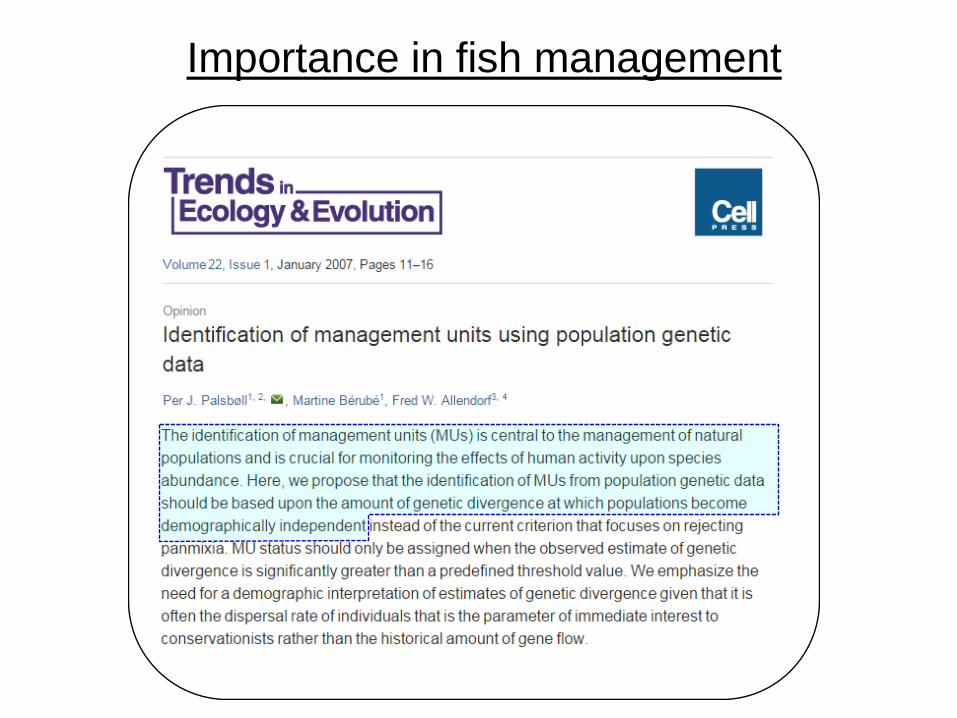
Importance in fish management

Population allele frequencies
Genetic composition of a population
Allele frequency - rate of occurrence of a gene variant (allele) at a particular locus

Population allele frequencies
Genetic composition of a population
High frequency - common alleles observed in many individuals in a population
Allele frequency - rate of occurrence of a gene variant (allele) at a particular locus

Low frequency - rare alleles observed in few individuals in a population
High frequency - common alleles observed in many individuals in a population
Population allele frequencies
Genetic composition of a population
Allele frequency - rate of occurrence of a gene variant (allele) at a particular locus
Population allele frequencies
Genetic composition of a population
Allele frequency - rate of occurrence of a gene variant (allele) at a particular locus
Evolution – change in allele frequencies over time

Population allele frequencies
Genetic composition of a population
Allele frequency - rate of occurrence of a gene variant (allele) at a particular locus
Evolution – change in allele frequencies over time
occurs at the population level.......Individuals do not evolve
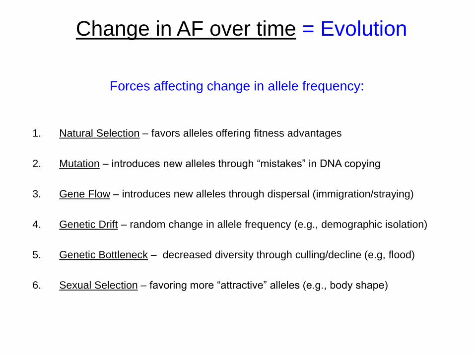
Change in AF over time = Evolution
Forces affecting change in allele frequency:
1. Natural Selection – favors alleles offering fitness advantages
2. Mutation – introduces new alleles through “mistakes” in DNA copying
3. Gene Flow – introduces new alleles through dispersal (immigration/straying)
4. Genetic Drift – random change in allele frequency (e.g., demographic isolation)
5. Genetic Bottleneck – decreased diversity through culling/decline (e.g, flood)
6. Sexual Selection – favoring more “attractive” alleles (e.g., body shape)

example: 12 Snake River steelhead
p q
q q
p p
p q p q
p q q q
q q
q q
q q q q
q q
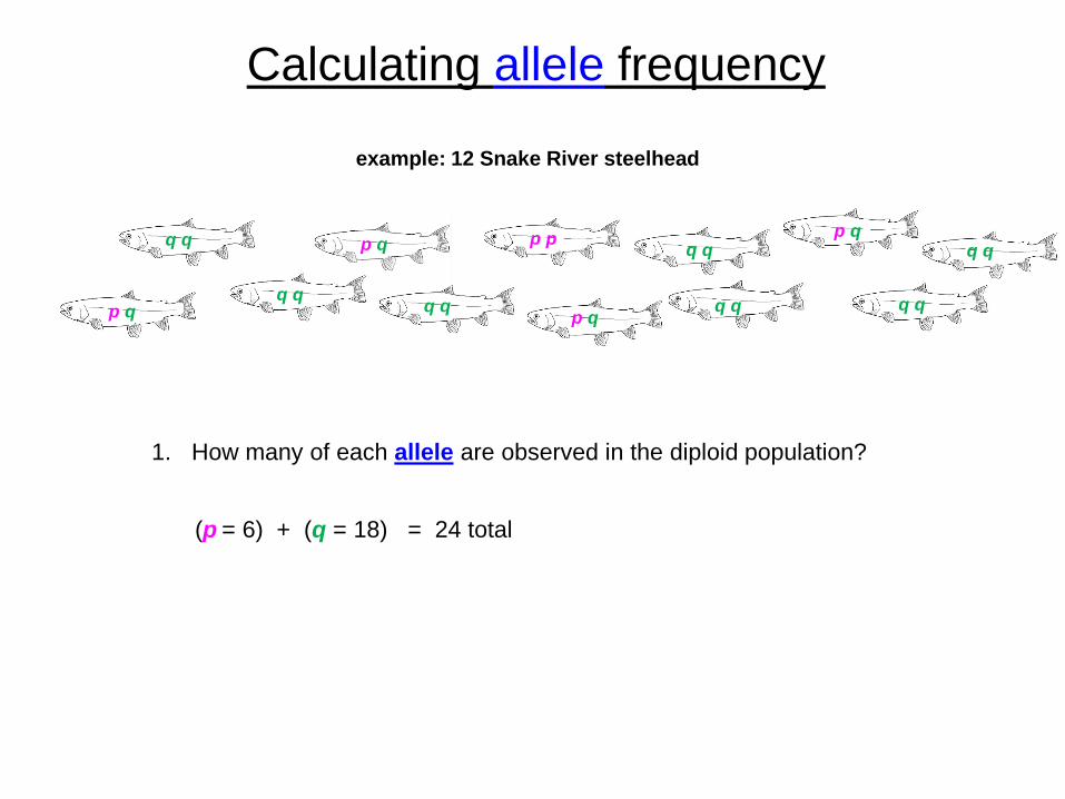
Calculating allele frequency
suppose there are two alleles p and q at gene X,
where frequency p + frequency q = 1
example: 12 Snake River steelhead
p q
q q
p p
p q p q
p q q q
q q
q q
q q q q
q q
1. How many of each allele are observed in the diploid population?
(p = 6) + (q = 18) = 24 total
Calculating allele frequency

2. What is the observed frequency of each allele in the population?
p = 6/24 = 0.25 q = 18/24 = 0.75 (sum = 1)
example: 12 Snake River steelhead
p q
q q
p p
p q p q
p q q q
q q
q q
q q q q
q q
1. How many of each allele are observed in the diploid population?
(p = 6) + (q = 18) = 24 total
Calculating allele frequency
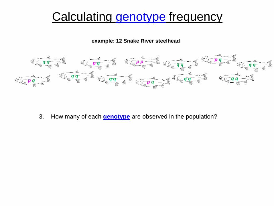
3. How many of each genotype are observed in the population?
Calculating genotype frequency
example: 12 Snake River steelhead
p q
q q
p p
p q p q
p q q q
q q
q q
q q q q
q q
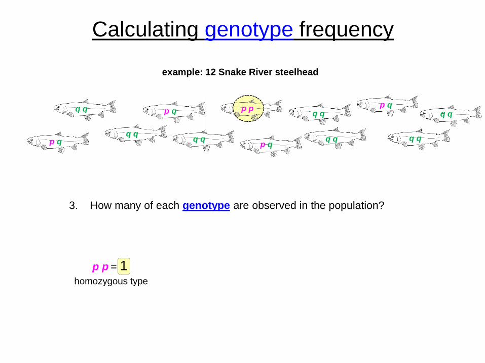
p p = 1 homozygous type
3. How many of each genotype are observed in the population?
example: 12 Snake River steelhead
p q
q q
p p
p q p q
p q q q
q q
q q
q q q q
q q
Calculating genotype frequency

p q = 4 heterozygous type
p p = 1 homozygous type
example: 12 Snake River steelhead
p q
q q
p p
p q p q
p q q q
q q
q q
q q q q
q q
3. How many of each genotype are observed in the population?
Calculating genotype frequency

example: 12 Snake River steelhead
p q
q q
p p
p q p q
p q q q
q q
q q
q q q q
q q
q q = 7 alternate homozygous type
p q = 4 heterozygous type
p p = 1 homozygous type
3. How many of each genotype are observed in the population?
Calculating genotype frequency

4. What is the observed frequency of each genotype in the population?
p p = 1 /12 = 0.083 p q = 4 /12 = 0.333 q q = 7 /12 = 0.583
0.083 + 0.333 + 0.583 = 1
example: 12 Snake River steelhead
p q
q q
p p
p q p q
p q q q
q q
q q
q q q q
q q
Calculating genotype frequency
Hardy-Weinberg Equilibrium (HWE)
• Fundamental principle (model, theorem, law) of population genetics
THE LAW: randomly mating populations maintain constant allele frequencies
and genotype frequencies from one generation to the next.
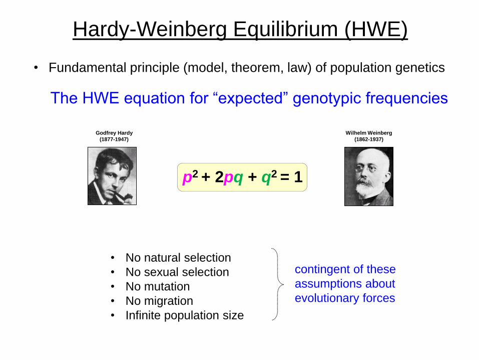
Hardy-Weinberg Equilibrium (HWE)
• Fundamental principle (model, theorem, law) of population genetics
The HWE equation for “expected” genotypic frequencies
• No natural selection
• No sexual selection
• No mutation
• No migration
• Infinite population size
contingent of these
assumptions about
evolutionary forces
p2 + 2pq + q2 = 1
Godfrey Hardy
(1877-1947)
Wilhelm Weinberg
(1862-1937)

Is our population in HWE?
example: 12 Snake River steelhead
p q
q q
p p
p q p q
p q q q
q q
q q
q q q q
q q

Is our population in HWE?
HWE equation: p2 + 2pq + q2 = 1
Our allele frequencies: p=0.25 q=0.75
example: 12 Snake River steelhead
p q
q q
p p
p q p q
p q q q
q q
q q
q q q q
q q
5. answer: does the observed deviate from the expected under HWE?

p2 = (0.25)2 = 0.063 expected frequency of pp
2pq = 2(0.25)(0.75) = 0.375 expected frequency of pq
q2 = (0.75)2 = 0.563 expected frequency of qq
Is our population in HWE?
HWE equation: p2 + 2pq + q2 = 1
Our allele frequencies: p=0.25 q=0.75
example: 12 Snake River steelhead
p q
q q
p p
p q p q
p q q q
q q
q q
q q q q
q q
5. answer: does the observed deviate from the expected under HWE?

6. Compare numbers of each genotype (observed & expected)
Is our population in HWE?
example: 12 Snake River steelhead
p q
q q
p p
p q p q
p q q q
q q
q q
q q q q
q q
x 12 = 0.8
x 12 = 4.5
x 12 = 6.8
(0.063)
(0.375)
(0.563)
# expected
pp
pq
x 12 = 1.0
x 12 = 4.0
x 12 = 7.0
(0.083)
(0.333)
(0.583)
# observed
pp
pq

7. Yes, statistically the population is in HWE, and we assume random mating
Is our population in HWE?
example: 12 Snake River steelhead
p q
q q
p p
p q p q
p q q q
q q
q q
q q q q
q q
1. No Natural Selection
2. No Sexual Selection
3. No mutation
4. No migration
5. Infinite population size
likely not absent
but nominal or static
P-value = 0.70
27
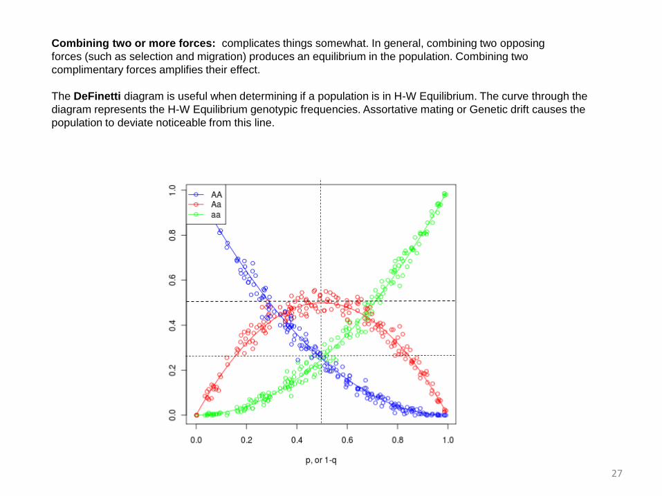
Combining two or more forces: complicates things somewhat. In general, combining two opposing
forces (such as selection and migration) produces an equilibrium in the population. Combining two
complimentary forces amplifies their effect.
The DeFinetti diagram is useful when determining if a population is in H-W Equilibrium. The curve through the
diagram represents the H-W Equilibrium genotypic frequencies. Assortative mating or Genetic drift causes the
population to deviate noticeable from this line.
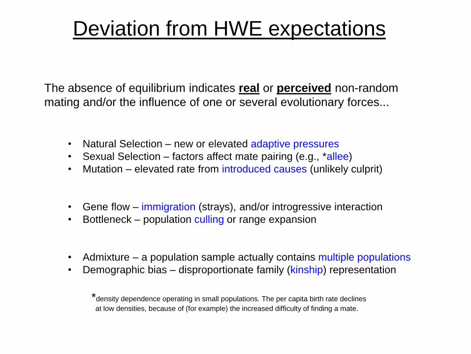
The absence of equilibrium indicates real or perceived non-random
mating and/or the influence of one or several evolutionary forces...
• Natural Selection – new or elevated adaptive pressures
• Sexual Selection – factors affect mate pairing (e.g., *allee)
• Mutation – elevated rate from introduced causes (unlikely culprit)
• Gene flow – immigration (strays), and/or introgressive interaction
• Bottleneck – population culling or range expansion
• Admixture – a population sample actually contains multiple populations
• Demographic bias – disproportionate family (kinship) representation
*density dependence operating in small populations. The per capita birth rate declines
at low densities, because of (for example) the increased difficulty of finding a mate.
Deviation from HWE expectations

Heterozygosity (HO or HE) - A measure of genetic variation across the genome.
The proportion of heterozygous (pq) individuals in a population.
Genetic Variation - The phenotypic and genotypic differences among individuals in a
population. Facilitates ability to adapt to changing environments
Genetic diversity/ variation
p q
q q
p p
p q p q
p q q q
q q
q q
q q q q
q q

Genetic diversity/ variation
• Relevance in fisheries harvest & management, supplementation & conservation
– Identification of stocks in mixtures
– Inbreeding, domestication, effective population size in hatcheries
– Diversity in life history and growth characteristics
– Difference in adaptive potential

• Amount of genetic variation between sub-populations:
High FST : divergence (restricted gene flow / isolation)
Low FST : similarity (gene flow / common origin)
Genetic distance: (FST)

• Amount of genetic variation between sub-populations:
High FST : divergence (restricted gene flow / isolation)
Low FST : similarity (gene flow / common origin)
HT = Total expected heterozygosity: sub-populations treated as one
HS = Average sub-population heterozygosity: ((2p1q1 + 2p2q2)/2)
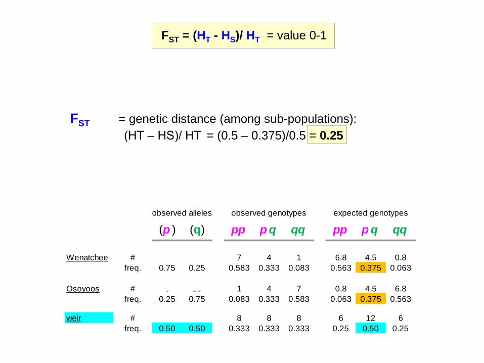
Genetic distance: (FST)
FST = (HT - HS)/ HT = value 0-1

Genetic distance: sockeye example
suppose we have 2 sub-population (n=12; 24 alleles)
Lake
Wenatchee
pp pp
pp
pp
pp pp
pp
pq
pq
pq
pq
Osoyoos Lake pp
pq
pq
pq
pq
qq qq qq
qq qq
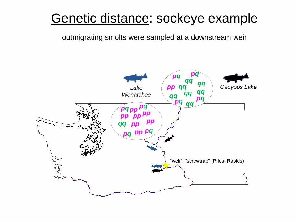
Genetic distance: sockeye example
outmigrating smolts were sampled at a downstream weir
Lake
Wenatchee
“weir”, “screwtrap” (Priest Rapids)
Osoyoos Lake
pp pp
pp
pp
pp pp
pp
pq
pq
pq
pq
pp
pq
pq
pq
pq
qq qq
qq qq
qq qq

12 individuals
24 alleles
(p ) (q) pp p q qq pp p q qq
Wenatchee # 18 6 7 4 1 6.8 4.5 0.8
freq. 0.75 0.25 0.583 0.333 0.083 0.563 0.375 0.063
Osoyoos # 6 18 1 4 7 0.8 4.5 6.8
freq. 0.25 0.75 0.083 0.333 0.583 0.063 0.375 0.563
weir # 12 12 8 8 8 6 12 6
freq. 0.50 0.50 0.333 0.333 0.333 0.250 0.500 0.250
observed genotypesobserved alleles expected genotypes
12 individuals
24 alleles
(p2 + 2pq + q2)
“expected” as per HWE

(p ) (q) pp p q qq pp p q qq
Wenatchee # 18 6 7 4 1 6.8 4.5 0.8
freq. 0.75 0.25 0.583 0.333 0.083 0.563 0.375 0.063
Osoyoos # 6 18 1 4 7 0.8 4.5 6.8
freq. 0.25 0.75 0.083 0.333 0.583 0.063 0.375 0.563
weir # 12 12 8 8 8 6 12 6
freq. 0.50 0.50 0.333 0.333 0.333 0.250 0.500 0.250
observed genotypesobserved alleles expected genotypes
Genetic distance: sockeye example
Wahlund effect: A reduction in heterozygosity caused by subpopulation structure
(p2 + 2pq + q2)
“expected” as per HWE

Genetic distance: sockeye example
Wahlund effect: A reduction in heterozygosity caused by subpopulation structure
• When two or more subpopulations have different allele frequencies the overall
heterozygosity is reduced even if the subpopulations are in HWE
(excess homozygotes, and loss of variation)
(p ) (q) pp p q qq pp p q qq
Wenatchee # 18 6 7 4 1 6.8 4.5 0.8
freq. 0.75 0.25 0.583 0.333 0.083 0.563 0.375 0.063
Osoyoos # 6 18 1 4 7 0.8 4.5 6.8
freq. 0.25 0.75 0.083 0.333 0.583 0.063 0.375 0.563
weir # 12 12 8 8 8 6 12 6
freq. 0.50 0.50 0.333 0.333 0.333 0.250 0.500 0.250
observed genotypesobserved alleles expected genotypes
(p2 + 2pq + q2)
“expected” as per HWE

(p ) (q) pp p q qq pp p q qq
Wenatchee # 18 6 7 4 1 6.8 4.5 0.8
freq. 0.75 0.25 0.583 0.333 0.083 0.563 0.375 0.063
Osoyoos # 6 18 1 4 7 0.8 4.5 6.8
freq. 0.25 0.75 0.083 0.333 0.583 0.063 0.375 0.563
weir # 12 12 8 8 8 6 12 6
freq. 0.50 0.50 0.333 0.333 0.333 0.25 0.50 0.25
observed genotypesobserved alleles expected genotypes
2(pq) = 2 * (0.5) * (0.5) = 0.5
HT = Total expected heterozygosity: sub-populations treated as one
FST = (HT - HS)/ HT = value 0-1

2(pq) = 2 * (0.5) * (0.5) = 0.5
HT = Total expected heterozygosity: sub-populations treated as one
FST = (HT - HS)/ HT = value 0-1
HS = Average sub-population heterozygosity
((2p1q1 + 2p2q2)/2) = ((2 * 0.375)+(2 * 0.375))/2 = 0.375
(p ) (q) pp p q qq pp p q qq
Wenatchee # 18 6 7 4 1 6.8 4.5 0.8
freq. 0.75 0.25 0.583 0.333 0.083 0.563 0.375 0.063
Osoyoos # 6 18 1 4 7 0.8 4.5 6.8
freq. 0.25 0.75 0.083 0.333 0.583 0.063 0.375 0.563
weir # 12 12 8 8 8 6 12 6
freq. 0.50 0.50 0.333 0.333 0.333 0.25 0.50 0.25
observed genotypesobserved alleles expected genotypes
FST = genetic distance (among sub-populations):
(HT – HS)/ HT = (0.5 – 0.375)/0.5 = 0.25
FST = (HT - HS)/ HT = value 0-1

42
Pairwise FST: sockeye example
Intermediate genetic distance – in the form of a half matrix
Alturas-LakeFishhook-CreekPettit-LakeRedfish-LakeStanley-LakeCreekWarm-LakeWallowaRiverWenatcheeSuttle10sockSuttle11sockSuttle09sockPelton10unkBilly10sockBilly11sockMetol10KOKMetol09KOKMeadow TUM04 TUM09 WELLS04 WELLS09 WHATCOM
0.000 Alturas-Lake
0.014 0.000 Fishhook-Creek
0.178 0.179 0.000 Pettit-Lake
0.078 0.090 0.261 0.000 Redfish-Lake
0.080 0.088 0.225 0.155 0.000 Stanley-LakeCreek
0.133 0.143 0.226 0.199 0.172 0.000 Warm-Lake
0.079 0.076 0.098 0.142 0.130 0.166 0.000 WallowaRiver
0.114 0.115 0.151 0.141 0.164 0.181 0.070 0.000 Wenatchee
0.130 0.134 0.049 0.192 0.165 0.182 0.043 0.098 0.000 Suttle10sock
0.123 0.126 0.060 0.187 0.162 0.180 0.036 0.088 0.004 0.000 Suttle11sock
0.123 0.128 0.056 0.185 0.161 0.181 0.037 0.094 0.003 0.002 0.000 Suttle09sock
0.103 0.107 0.098 0.156 0.149 0.181 0.026 0.051 0.030 0.022 0.023 0.000 Pelton10unk
0.094 0.099 0.093 0.143 0.142 0.171 0.024 0.048 0.030 0.020 0.024 0.007 0.000 Billy10sock
0.096 0.099 0.092 0.148 0.140 0.167 0.023 0.050 0.028 0.019 0.022 0.007 0.003 0.000 Billy11sock
0.095 0.101 0.098 0.146 0.139 0.168 0.024 0.045 0.032 0.022 0.026 0.007 0.003 0.003 0.000 Metol10KOK
0.093 0.097 0.094 0.144 0.139 0.166 0.023 0.047 0.030 0.020 0.024 0.006 0.003 0.002 0.002 0.000 Metol09KOK
0.093 0.090 0.124 0.181 0.155 0.192 0.030 0.107 0.083 0.078 0.077 0.070 0.067 0.065 0.064 0.066 0.000 Meadow
0.117 0.119 0.153 0.135 0.165 0.187 0.076 0.003 0.100 0.091 0.097 0.056 0.051 0.053 0.048 0.050 0.111 0.000 TUM04
0.114 0.114 0.147 0.136 0.164 0.179 0.073 0.002 0.098 0.089 0.095 0.054 0.050 0.052 0.047 0.049 0.110 0.002 0.000 TUM09
0.054 0.058 0.133 0.088 0.116 0.140 0.060 0.051 0.093 0.085 0.088 0.060 0.056 0.057 0.055 0.054 0.086 0.052 0.051 0.000 WELLS04
0.058 0.059 0.132 0.092 0.119 0.144 0.060 0.047 0.092 0.084 0.087 0.059 0.055 0.056 0.054 0.053 0.088 0.048 0.047 0.003 0.000 WELLS09
0.154 0.159 0.035 0.230 0.191 0.205 0.073 0.123 0.019 0.030 0.028 0.069 0.068 0.066 0.069 0.068 0.101 0.123 0.121 0.115 0.114 0.000 WHATCOM

43
Pairwise FST: sockeye example
Intermediate genetic distance – in the form of a dendrogram (Neighbor-Joining Tree)
Fishhook
Alturas Lake
Redfish Lake
Stanley Lake Cr.
Warm Lake
Okanogan
Wenatchee
Wallowa Lake (stream)
Meadow Cr.
Pelton (2011)
Pelton (2012)
Metolius (2012)
Lake Billy Chinook (2010)
Pelton (2010)
Wallow Lake (shore)
Wickiup
Odell
Palmer
Pettit Lake
Whatcom Lake
Suttle Lake (2011)
Link Creek
Paulina Lake
Wizard Falls
Metolius (2009)
Metolius (2010)
Lake Billy Chinook (2011)
Suttle Lake (2009)
Suttle Lake (2010)
62
100
50
68
84
91
90
52
89
94
100
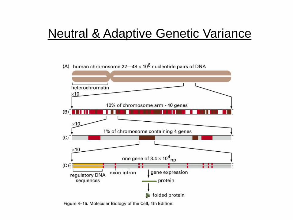
Neutral & Adaptive Genetic Variance

• Genetic variation that has no effect on fitness
– Genetic variation that typically occurs in non-coding regions
of the genome (introns etc.), and therefore does not change
proteins or expression of a gene (variation in the DNA sequence
that does not translate to variation in physiological response)
– Variation that is not under the influence of selective pressures
(degree of neutral variance is not contingent on natural selection)
– Does not violate HWE assumptions
Neutral genetic variance

• Genetic variation that may effect individual fitness
– Genetic variation that typically occurs in coding regions
of the genome (exons etc.), and therefore can change
proteins or expression of a gene (variation in the DNA sequence
that translates to variation in physiological response: MHC
polymorphism and immunity)
– Variation that may be under the influence of selective pressures
(degree of adaptive variance is subject to forces of evolution –
natural selection)
– Violates HWE assumptions, likely to cause deviation from HWE
Adaptive genetic variance

Population Genetics EXERCISE
http://www.radford.edu/~rsheehy/Gen_flash/popgen/