introduction to probability - mcgill university

9

Conditional expectation

Given that you’ve read the earlier chapters, you already know what conditionalexpectation is: expectation, but using conditional probabilities. This is an essentialconcept, for reasons analogous to why we need conditional probability:

• Conditional expectation is a powerful tool for calculating expectations. Usingstrategies such as conditioning on what we wish we knew and first-step analysis,we can often decompose complicated expectation problems into simpler pieces.

• Conditional expectation is a relevant quantity in its own right, allowing us topredict or estimate unknowns based on whatever evidence is currently available.For example, in statistics we often want to predict a response variable (such astest scores or earnings) based on explanatory variables (such as number of practiceproblems solved or enrollment in a job training program).

There are two di↵erent but closely linked notions of conditional expectation:

• Conditional expectation E(Y |A) given an event : let Y be an r.v., and A be anevent. If we learn that A occurred, our updated expectation for Y is denoted byE(Y |A) and is computed analogously to E(Y ), except using conditional probabil-ities given A.

• Conditional expectation E(Y |X) given a random variable: a more subtle questionis how to define E(Y |X), where X and Y are both r.v.s. Intuitively, E(Y |X) isthe r.v. that best predicts Y using only the information available from X.

In this chapter, we explore the definitions, properties, intuitions, and applicationsof both forms of conditional expectation.

9.1 Conditional expectation given an event

Recall that the expectation E(Y ) of a discrete r.v. Y is a weighted average of itspossible values, where the weights are the PMF values P (Y = y). After learningthat an event A occurred, we want to use weights that have been updated to reflectthis new information. The definition of E(Y |A) simply replaces the probabilityP (Y = y) with the conditional probability P (Y = y|A).

383

384 Introduction to Probability

Similarly, if Y is continuous, E(Y ) is still a weighted average of the possible valuesof Y , with an integral in place of a sum and the PDF value f(y) in place of a PMFvalue. If we learn that A occurred, we update the expectation for Y by replacingf(y) with the conditional PDF f(y|A).

Definition 9.1.1 (Conditional expectation given an event). Let A be an eventwith positive probability. If Y is a discrete r.v., then the conditional expectation ofY given A is

E(Y |A) =X

y

yP (Y = y|A),

where the sum is over the support of Y . If Y is a continuous r.v. with PDF f , then

E(Y |A) =

Z 1

�1yf(y|A)dy,

where the conditional PDF f(y|A) is defined as the derivative of the conditionalCDF F (y|A) = P (Y y|A), and can also be computed by a hybrid version ofBayes’ rule:

f(y|A) =P (A|Y = y)f(y)

P (A).

Intuition 9.1.2. To gain intuition for E(Y |A), let’s consider approximating itvia simulation (or via the frequentist perspective, based on repeating the sameexperiment many times). Imagine generating a large number n of replications of theexperiment for which Y is a numerical summary. We then have Y -values y1, . . . , yn,and we can approximate

E(Y ) ⇡ 1

n

nX

j=1

yj .

To approximate E(Y |A), we restrict to the replications where A occurred, andaverage only those Y -values. This can be written as

E(Y |A) ⇡P

n

j=1 yjIj ,Pn

j=1 Ij,

where Ij is the indicator of A occurring in the jth replication. This is undefinedif A never occurred in the simulation, which makes sense since then there is nosimulation data about what the “A occurred” scenario is like. We would like tohave n large enough so that there are many occurrences of A (if A is a rare event,more sophisticated techniques for approximating E(Y |A) may be needed).

The principle is simple though: E(Y |A) is approximately the average of Y in a largenumber of simulation runs in which A occurred. ⇤h 9.1.3. Confusing conditional expectation and unconditional expectation is adangerous mistake. More generally, not keeping careful track of what you should beconditioning on and what you are conditioning on is a recipe for disaster.

Conditional expectation 385

For a life-or-death example of the previous biohazard, consider life expectancy.

Example 9.1.4 (Life expectancy). Fred is 30 years old, and he hears that theaverage life expectancy in his country is 80 years. Should he conclude that, onaverage, he has 50 years of life left? No, there is a crucial piece of information thathe must condition on: the fact that he has lived to age 30 already. Letting T beFred’s lifespan, we have the cheerful news that

E(T ) < E(T |T � 30).

The left-hand side is Fred’s life expectancy at birth (it implicitly conditions on thefact that he is born), and the right-hand side is Fred’s life expectancy given that hereaches age 30.

A harder question is how to decide on an appropriate estimate to use for E(T ). Isit just 80, the overall average for his country? In almost every country, women havea longer average life expectancy than men, so it makes sense to condition on Fredbeing a man. But should we also condition on what city he was born in? Should wecondition on racial and financial information about his parents, or the time of daywhen he was born? Intuitively, we would like estimates that are both accurate andrelevant for Fred, but there is a tradeo↵ since if we condition on more characteristicsof Fred, then there are fewer people who match those characteristics to use as datafor estimating the life expectancy.

Now consider some specific numbers for the United States. A Social Security Admin-istration study estimated that between 1900 and 2000, the average life expectancyat birth in the U.S. for men increased from 46 to 74, and for women increased from49 to 79. Tremendous gains! But most of the gains are due to decreases in childmortality. For a 30-year-old person in 1900, the average number of years remainingwas 35 for a man and 36 for a woman (bringing their conditional life expectanciesto 65 and 66); in 2000, the corresponding numbers are 46 for a man and 50 for awoman.

There are some subtle statistical issues in obtaining these estimates. For example,how were estimates for life expectancy for someone born in 2000 obtained withoutwaiting at least until the year 2100? Estimating distributions for survival is a veryimportant topic in biostatistics and actuarial science. ⇤

The law of total probability allows us to get unconditional probabilities by slicingup the sample space and computing conditional probabilities in each slice. The sameidea works for computing unconditional expectations.

Theorem 9.1.5 (Law of total expectation). Let A1, . . . , An be a partition of asample space, with P (Ai) > 0 for all i, and let Y be a random variable on thissample space. Then

E(Y ) =nX

i=1

E(Y |Ai)P (Ai).


In fact, since all probabilities are expectations by the fundamental bridge, the lawof total probability is a special case of the law of total expectation. To see this, letY = IB for an event B; then the above theorem says

P (B) = E(IB) =nX

i=1

E(IB|Ai)P (Ai) =nX

i=1

P (B|Ai)P (Ai),

which is exactly LOTP. The law of total expectation is, in turn, a special case of amajor result called Adam’s law (Theorem 9.3.7), so we will not prove it yet.

There are many interesting examples of using wishful thinking to break up an un-conditional expectation into conditional expectations. We begin with two cautionarytales about the importance of conditioning carefully and not destroying informationwithout justification.

Example 9.1.6 (Two-envelope paradox). A stranger presents you with twoidentical-looking, sealed envelopes, each of which contains a check for some pos-itive amount of money. You are informed that one of the envelopes contains exactlytwice as much money as the other. You can choose either envelope. Which do youprefer: the one on the left or the one on the right? (Assume that the expectedamount of money in each envelope is finite—certainly a good assumption in the realworld!)

X Y

FIGURE 9.1

Two envelopes, where one contains twice as much money as the other. Either Y =2X or Y = X/2, with equal probabilities. Which would you prefer?

Solution:

Let X and Y be the amounts in the left and right envelopes, respectively. Bysymmetry, there is no reason to prefer one envelope over the other (we are assumingthere is no prior information that the stranger is left-handed and left-handed peopleprefer putting more money on the left). Concluding by symmetry that E(X) =E(Y ), it seems that you should not care which envelope you get.

But as you daydream about what’s inside the envelopes, another argument occursto you: suppose that the left envelope has $100. Then the right envelope either has$50 or $200. The average of $50 and $200 is $125, so it seems then that the rightenvelope is better. But there was nothing special about $100 here; for any value x

for the left envelope, the average of 2x and x/2 is greater than x, suggesting thatthe right envelope is better. This is bizarre though, since not only does it contradict


the symmetry argument, but also the same reasoning could be applied starting withthe right envelope, leading to switching back and forth forever!

Let us try to formalize this argument to see what’s going on. We have Y = 2X orY = X/2, with equal probabilities. By Theorem 9.1.5,

E(Y ) = E(Y |Y = 2X) · 1

2+ E

�Y |Y = X/2

�· 1

2.

One might then think that this is

E(2X) · 1

2+ E

�X/2

�· 1

2=

5

4E(X),

suggesting a 25% gain from switching from the left to the right envelope. But thereis a blunder in that calculation: E(Y |Y = 2X) = E(2X|Y = 2X), but there is nojustification for dropping the Y = 2X condition after plugging in 2X for Y .

To put it another way, let I be the indicator of the event Y = 2X, so that E(Y |Y =2X) = E(2X|I = 1). If we know that X is independent of I, then we can drop thecondition I = 1. But in fact we have just proven that X and I can’t be independent:if they were, we’d have a paradox! Surprisingly, observing X gives information aboutwhether X is the bigger value or the smaller value. If we learn that X is very large,we might guess that X is larger than Y , but what is considered very large? Is 1012

very large, even though it is tiny compared with 10100? The two-envelope paradoxsays that no matter what the distribution of X is, there are reasonable ways todefine “very large” relative to that distribution.

In Exercise 7 you will look at a related problem, in which the amounts of moneyin the two envelopes are i.i.d. random variables. You’ll show that if you are allowedto look inside one of the envelopes and then decide whether to switch, there is astrategy that allows you to get the better envelope more than 50% of the time! ⇤

The next example vividly illustrates the importance of conditioning on all the in-formation. The phenomenon revealed here arises in many real-life decisions aboutwhat to buy and what investments to make.

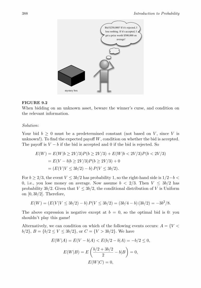
Example 9.1.7 (Mystery prize). You are approached by another stranger, whogives you an opportunity to bid on a mystery box containing a mystery prize! Thevalue of the prize is completely unknown, except that it is worth at least nothing,and at most a million dollars. So the true value V of the prize is considered to beUniform on [0,1] (measured in millions of dollars).

You can choose to bid any amount b (in millions of dollars). You have the chance toget the prize for considerably less than it is worth, but you could also lose moneyif you bid too much. Specifically, if b < 2V/3, then the bid is rejected and nothingis gained or lost. If b � 2V/3, then the bid is accepted and your net payo↵ is V � b

(since you pay b to get a prize worth V ). What is your optimal bid b, to maximizethe expected payo↵?


Bid $250,000? If it's rejected, I lose nothing. If it's accepted, I get a prize worth $500,000 on

average!

mystery box

FIGURE 9.2

When bidding on an unknown asset, beware the winner’s curse, and condition onthe relevant information.

Solution:

Your bid b � 0 must be a predetermined constant (not based on V , since V isunknown!). To find the expected payo↵ W , condition on whether the bid is accepted.The payo↵ is V � b if the bid is accepted and 0 if the bid is rejected. So

E(W ) = E(W |b � 2V/3)P (b � 2V/3) + E(W |b < 2V/3)P (b < 2V/3)

= E(V � b|b � 2V/3)P (b � 2V/3) + 0

= (E(V |V 3b/2) � b) P (V 3b/2).

For b � 2/3, the event V 3b/2 has probability 1, so the right-hand side is 1/2�b <

0, i.e., you lose money on average. Now assume b < 2/3. Then V 3b/2 hasprobability 3b/2. Given that V 3b/2, the conditional distribution of V is Uniformon [0, 3b/2]. Therefore,

E(W ) = (E(V |V 3b/2) � b) P (V 3b/2) = (3b/4 � b) (3b/2) = �3b2/8.

The above expression is negative except at b = 0, so the optimal bid is 0: youshouldn’t play this game!

Alternatively, we can condition on which of the following events occurs: A = {V <

b/2}, B = {b/2 V 3b/2}, or C = {V > 3b/2}. We have

E(W |A) = E(V � b|A) < E(b/2 � b|A) = �b/2 0,

E(W |B) = E

✓b/2 + 3b/2

2� b|B

◆= 0,

E(W |C) = 0,


so we should just set b = 0 and walk away.

The moral of this story is to condition on all the information. It is crucial in theabove calculation to use E(V |V 3b/2) rather than E(V ) = 1/2; knowing that thebid was accepted gives information about how much the mystery prize is worth, sowe shouldn’t destroy that information. This problem is related to the so-called win-ner’s curse, which says that the winner in an auction with incomplete informationtends to profit less than they expect (unless they understand probability!). This isbecause in many settings, the expected value of the item that they bid on giventhat they won the bid is less than the unconditional expected value they originallyhad in mind. For b � 2/3, conditioning on V 3b/2 does nothing since we knowin advance that V 1, but such a bid is ludicrously high. For any b < 2/3, findingout that your bid is accepted lowers your expectation:

E(V |V 3b/2) < E(V ).

⇤The remaining examples use first-step analysis to calculate unconditional expecta-tions. First, as promised in Chapter 4, we derive the expectation of the Geometricdistribution using first-step analysis.

Example 9.1.8 (Geometric expectation redux). Let X ⇠ Geom(p). Interpret X asthe number of Tails before the first Heads in a sequence of coin flips with probabilityp of Heads. To get E(X), we condition on the outcome of the first toss: if it landsHeads, then X is 0 and we’re done; if it lands Tails, then we’ve wasted one toss andare back to where we started, by memorylessness. Therefore,

E(X) = E(X|first toss H) · p + E(X|first toss T ) · q

= 0 · p + (1 + E(X)) · q,

which gives E(X) = q/p. ⇤The next example derives expected waiting times for some more complicated pat-terns, using two steps of conditioning.

Example 9.1.9 (Time until HH vs. HT ). You toss a fair coin repeatedly. Whatis the expected number of tosses until the pattern HT appears for the first time?What about the expected number of tosses until HH appears for the first time?

Solution:

Let WHT be the number of tosses until HT appears. As we can see from Figure9.3, WHT is the waiting time for the first Heads, which we’ll call W1, plus theadditional waiting time for the first Tails after the first Heads, which we’ll call W2.By the story of the First Success distribution, W1 and W2 are i.i.d. FS(1/2), soE(W1) = E(W2) = 2 and E(WHT ) = 4.

Finding the expected waiting time for HH, E(WHH), is more complicated. We can’t


TTTHHHHTHHT...

W1 W2

FIGURE 9.3

Waiting time for HT is the waiting time for the first Heads, W1, plus the additionalwaiting time for the next Tails, W2. Durable partial progress is possible!

apply the same logic as for E(WHT ): as shown in Figure 9.4, if the first Heads isimmediately followed by Tails, our progress is destroyed and we must start fromscratch. But this is progress for us in solving the problem, since the fact that thesystem can get reset suggests the strategy of first-step analysis. Let’s condition onthe outcome of the first toss:

E(WHH) = E(WHH |first toss H)1

2+ E(WHH |first toss T )

1

2.

THTTTTHHHH...

start over

FIGURE 9.4

When waiting for HH, partial progress can easily be destroyed.

For the second term, E(WHH |first toss T) = 1 + E(WHH) by memorylessness. Forthe first term, we compute E(WHH |1st toss H) by further conditioning on the out-come of the second toss. If the second toss is Heads, we have obtained HH in twotosses. If the second toss is Tails, we’ve wasted two tosses and have to start all over!This gives

E(WHH |first toss H) = 2 · 1

2+ (2 + E(WHH)) · 1

2.

Therefore,

E(WHH) =

✓2 · 1

2+ (2 + E(WHH)) · 1

2

◆1

2+ (1 + E(WHH))

1

2.

Solving for E(WHH), we get E(WHH) = 6.

It might seem surprising at first that the expected waiting time for HH is greaterthan the expected waiting time for HT. How do we reconcile this with the fact that


in two tosses of the coin, HH and HT both have a 1/4 chance of appearing? Whyaren’t the average waiting times the same by symmetry?

As we solved this problem, we in fact noticed an important asymmetry. Whenwaiting for HT, once we get the first Heads, we’ve achieved partial progress thatcannot be destroyed: if the Heads is followed by another Heads, we’re in the sameposition as before, and if the Heads is followed by a Tails, we’re done. By contrast,when waiting for HH, even after getting the first Heads, we could be sent back tosquare one if the Heads is followed by a Tails. This suggests the average waitingtime for HH should be longer. Symmetry implies that the average waiting time forHH is the same as that for TT, and that for HT is the same as that for TH, but itdoes not imply that the average waiting times for HH and HT are the same.

More intuition into what’s going on can be obtained by considering a long stringof coin flips, as in Figure 9.5. We notice right away that appearances of HH canoverlap, while appearances of HT must be disjoint. Since there are the same averagenumber of HH s and HT s, but HH s clump together while HT s do not, the spacingbetween successive strings of HH s must be greater to compensate.

HHTHHTTHHHHTHTHTTHTT

HHTHHTTHHHHTHTHTTHTT

FIGURE 9.5

Clumping. (a) Appearances of HH can overlap. (b) Appearances of HT must bedisjoint.

Related problems occur in information theory when compressing a message, and ingenetics when looking for recurring patterns (called motifs) in DNA sequences. ⇤Our final example in this section uses wishful thinking for both probabilities andexpectations to study a question about a random walk.

Example 9.1.10 (Random walk on the integers). An immortal drunk man wandersaround randomly on the integers. He starts at the origin, and at each step he moves1 unit to the right or 1 unit to the left, with equal probabilities, independently of allhis previous steps. Let b be a googolplex (this is 10g, where g = 10100 is a googol).

(a) Find a simple expression for the probability that the immortal drunk visits b

before returning to the origin for the first time.

(b) Find the expected number of times that the immortal drunk visits b beforereturning to the origin for the first time.

Solution:

(a) Let B be the event that the drunk man visits b before returning to the origin


for the first time and let L be the event that his first move is to the left. ThenP (B|L) = 0 since any path from �1 to b must pass through 0. For P (B|Lc), we areexactly in the setting of the gambler’s ruin problem, where player A starts with $1,player B starts with $(b�1), and the rounds are fair. Applying that result, we have

P (B) = P (B|L)P (L) + P (B|Lc)P (Lc) =1

b· 1

2=

1

2b.

(b) Let N be the number of visits to b before returning to the origin for the firsttime, and let p = 1/(2b) be the probability found in (a). Then

E(N) = E(N |N = 0)P (N = 0) + E(N |N � 1)P (N � 1) = pE(N |N � 1).

The conditional distribution of N given N � 1 is FS(p): given that the man reachesb, by symmetry there is probability p of returning to the origin before visiting b again(call this “success”) and probability 1 � p of returning to b again before returningto the origin (call this “failure”). Note that the trials are independent since thesituation is the same each time he is at b, independent of the past history. ThusE(N |N � 1) = 1/p, and

E(N) = pE(N |N � 1) = p · 1

p= 1.

Surprisingly, the result doesn’t depend on the value of b, and our proof didn’t requireknowing the value of p. ⇤

9.2 Conditional expectation given an r.v.

In this section we introduce conditional expectation given a random variable. Thatis, we want to understand what it means to write E(Y |X) for an r.v. X. We will seethat E(Y |X) is a random variable that is, in a certain sense, our best prediction ofY , assuming we get to know X.

The key to understanding E(Y |X) is first to understand E(Y |X = x). Since X = x

is an event, E(Y |X = x) is just the conditional expectation of Y given this event,and it can be computed using the conditional distribution of Y given X = x.

If Y is discrete, we use the conditional PMF P (Y = y|X = x) in place of theunconditional PMF P (Y = y):

E(Y |X = x) =X

y

yP (Y = y|X = x).

Analogously, if Y is continuous, we use the conditional PDF fY |X(y|x) in place ofthe unconditional PDF:

E(Y |X = x) =

Z 1

�1yfY |X(y|x)dy.


Notice that because we sum or integrate over y, E(Y |X = x) is a function of x

only. We can give this function a name, like g: let g(x) = E(Y |X = x). We defineE(Y |X) as the random variable obtained by finding the form of the function g(x),then plugging in X for x.

Definition 9.2.1 (Conditional expectation given an r.v.). Let g(x) = E(Y |X = x).Then the conditional expectation of Y given X, denoted E(Y |X), is defined to be therandom variable g(X). In other words, if after doing the experiment X crystallizesinto x, then E(Y |X) crystallizes into g(x).

h 9.2.2. The notation in this definition sometimes causes confusion. It does notsay “g(x) = E(Y |X = x), so g(X) = E(Y |X = X), which equals E(Y ) becauseX = X is always true”. Rather, we should first compute the function g(x), thenplug in X for x. For example, if g(x) = x

2, then g(X) = X2. A similar biohazard is

h 5.3.2, about the meaning of F (X) in the Universality of the Uniform.

h 9.2.3. By definition, E(Y |X) is a function of X, so it is a random variable.Thus it makes sense to compute quantities like E(E(Y |X)) and Var(E(Y |X)), themean and variance of the r.v. E(Y |X). It is easy to be ensnared by category errorswhen working with conditional expectation, so we should always keep in mind thatconditional expectations of the form E(Y |A) are numbers, while those of the formE(Y |X) are random variables.

Here are some quick examples of how to calculate conditional expectation. In bothexamples, we don’t need to do a sum or integral to get E(Y |X = x) because a moredirect approach is available.

Example 9.2.4. Suppose we have a stick of length 1 and break the stick at apoint X chosen uniformly at random. Given that X = x, we then choose anotherbreakpoint Y uniformly on the interval [0, x]. Find E(Y |X), and its mean andvariance.

Solution:

From the description of the experiment, X ⇠ Unif(0, 1) and Y |X = x ⇠ Unif(0, x).Then E(Y |X = x) = x/2, so by plugging in X for x, we have

E(Y |X) = X/2.

The expected value of E(Y |X) is

E(E(Y |X)) = E(X/2) = 1/4.

(We will show in the next section that a general property of conditional expectationis that E(E(Y |X)) = E(Y ), so it also follows that E(Y ) = 1/4.) The variance ofE(Y |X) is

Var(E(Y |X)) = Var(X/2) = 1/48.

⇤


Example 9.2.5. For X, Yi.i.d.⇠ Expo(�), find E(max(X, Y )| min(X, Y )).

Solution:

Let M = max(X, Y ) and L = min(X, Y ). By the memoryless property, M � L isindependent of L, and M � L ⇠ Expo(�) (see Example 7.3.6). Therefore

E(M |L = l) = E(L|L = l) + E(M � L|L = l) = l + E(M � L) = l +1

�,

and E(M |L) = L + 1�. ⇤

9.3 Properties of conditional expectation

Conditional expectation has some very useful properties, that often allow us to solveproblems without having to go all the way back to the definition.

• Dropping what’s independent: If X and Y are independent, then E(Y |X) = E(Y ).

• Taking out what’s known: For any function h, E(h(X)Y |X) = h(X)E(Y |X).

• Linearity: E(Y1 + Y2|X) = E(Y1|X) + E(Y2|X), and E(cY |X) = cE(Y |X) for c aconstant (the latter is a special case of taking out what’s known).

• Adam’s law: E(E(Y |X)) = E(Y ).

• Projection interpretation: The r.v. Y � E(Y |X), which is called the residual fromusing X to predict Y , is uncorrelated with h(X) for any function h.

Let’s discuss each property individually.

Theorem 9.3.1 (Dropping what’s independent). If X and Y are independent, thenE(Y |X) = E(Y ).

This is true because independence implies E(Y |X = x) = E(Y ) for all x, henceE(Y |X) = E(Y ). Intuitively, if X provides no information about Y , then our bestguess for Y , even if we get to know X, is still the unconditional mean E(Y ). However,the converse is false: a counterexample is given in Example 9.3.3 below.

Theorem 9.3.2 (Taking out what’s known). For any function h,

E(h(X)Y |X) = h(X)E(Y |X).

Intuitively, when we take expectations given X, we are treating X as if it hascrystallized into a known constant. Then any function of X, say h(X), also acts likea known constant while we are conditioning on X. Taking out what’s known is theconditional version of the unconditional fact that E(cY ) = cE(Y ). The di↵erence isthat E(cY ) = cE(Y ) asserts that two numbers are equal, while taking out what’sknown asserts that two random variables are equal.


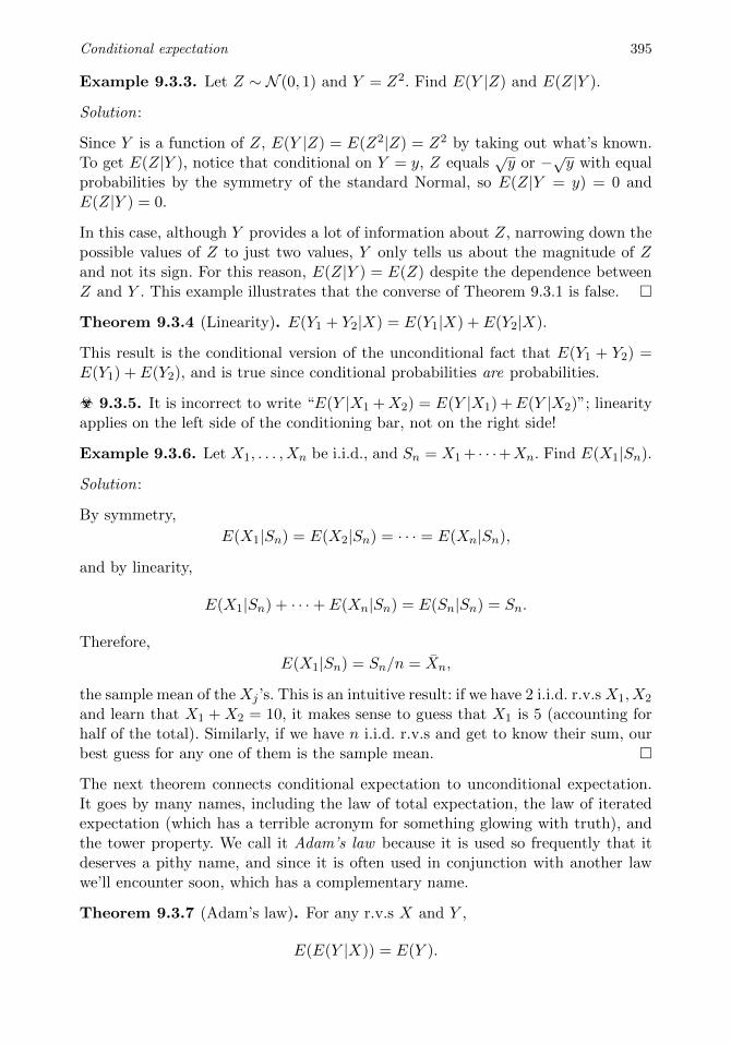
Example 9.3.3. Let Z ⇠ N (0, 1) and Y = Z2. Find E(Y |Z) and E(Z|Y ).

Solution:

Since Y is a function of Z, E(Y |Z) = E(Z2|Z) = Z2 by taking out what’s known.

To get E(Z|Y ), notice that conditional on Y = y, Z equalsp

y or �py with equal

probabilities by the symmetry of the standard Normal, so E(Z|Y = y) = 0 andE(Z|Y ) = 0.

In this case, although Y provides a lot of information about Z, narrowing down thepossible values of Z to just two values, Y only tells us about the magnitude of Z

and not its sign. For this reason, E(Z|Y ) = E(Z) despite the dependence betweenZ and Y . This example illustrates that the converse of Theorem 9.3.1 is false. ⇤

Theorem 9.3.4 (Linearity). E(Y1 + Y2|X) = E(Y1|X) + E(Y2|X).

This result is the conditional version of the unconditional fact that E(Y1 + Y2) =E(Y1) + E(Y2), and is true since conditional probabilities are probabilities.

h 9.3.5. It is incorrect to write “E(Y |X1 + X2) = E(Y |X1) + E(Y |X2)”; linearityapplies on the left side of the conditioning bar, not on the right side!

Example 9.3.6. Let X1, . . . , Xn be i.i.d., and Sn = X1 + · · ·+Xn. Find E(X1|Sn).

Solution:

By symmetry,

E(X1|Sn) = E(X2|Sn) = · · · = E(Xn|Sn),

and by linearity,

E(X1|Sn) + · · · + E(Xn|Sn) = E(Sn|Sn) = Sn.

Therefore,

E(X1|Sn) = Sn/n = Xn,

the sample mean of the Xj ’s. This is an intuitive result: if we have 2 i.i.d. r.v.s X1, X2

and learn that X1 + X2 = 10, it makes sense to guess that X1 is 5 (accounting forhalf of the total). Similarly, if we have n i.i.d. r.v.s and get to know their sum, ourbest guess for any one of them is the sample mean. ⇤

The next theorem connects conditional expectation to unconditional expectation.It goes by many names, including the law of total expectation, the law of iteratedexpectation (which has a terrible acronym for something glowing with truth), andthe tower property. We call it Adam’s law because it is used so frequently that itdeserves a pithy name, and since it is often used in conjunction with another lawwe’ll encounter soon, which has a complementary name.

Theorem 9.3.7 (Adam’s law). For any r.v.s X and Y ,

E(E(Y |X)) = E(Y ).


Proof. We present the proof in the case where X and Y are both discrete (theproofs for other cases are analogous). Let E(Y |X) = g(X). We proceed by applyingLOTUS, expanding the definition of g(x) to get a double sum, and then swappingthe order of summation:

E(g(X)) =X

x

g(x)P (X = x)

=X

x

X

y

yP (Y = y|X = x)

!P (X = x)

=X

x

X

y

yP (X = x)P (Y = y|X = x)

=X

y

y

X

x

P (X = x, Y = y)

=X

y

yP (Y = y) = E(Y ).

⌅

Adam’s law is a more compact, more general version of the law of total expectation(Theorem 9.1.5). For X discrete, the statements

E(Y ) =X

x

E(Y |X = x)P (X = x)

and

E(Y ) = E(E(Y |X))

mean the same thing, since if we let E(Y |X = x) = g(x), then

E(E(Y |X)) = E(g(X)) =X

x

g(x)P (X = x) =X

x

E(Y |X = x)P (X = x).

But the Adam’s law expression is shorter and applies just as well in the continuouscase.

Armed with Adam’s law, we have a powerful strategy for finding an expectationE(Y ), by conditioning on an r.v. X that we wish we knew. First obtain E(Y |X) bytreating X as known, and then take the expectation of E(Y |X). We will see variousexamples of this later in the chapter.

Just as there are forms of Bayes’ rule and LOTP with extra conditioning, as dis-cussed in Chapter 2, there is a version of Adam’s law with extra conditioning.

Theorem 9.3.8 (Adam’s law with extra conditioning). For any r.v.s X,Y, Z, wehave

E(E(Y |X, Z)|Z) = E(Y |Z).


The above equation is Adam’s law, except with extra conditioning on Z insertedeverywhere. It is true because conditional probabilities are probabilities. So weare free to use Adam’s law to help us find both unconditional expectations andconditional expectations.

Using Adam’s law, we can also prove the last item on our list of properties ofconditional expectation.

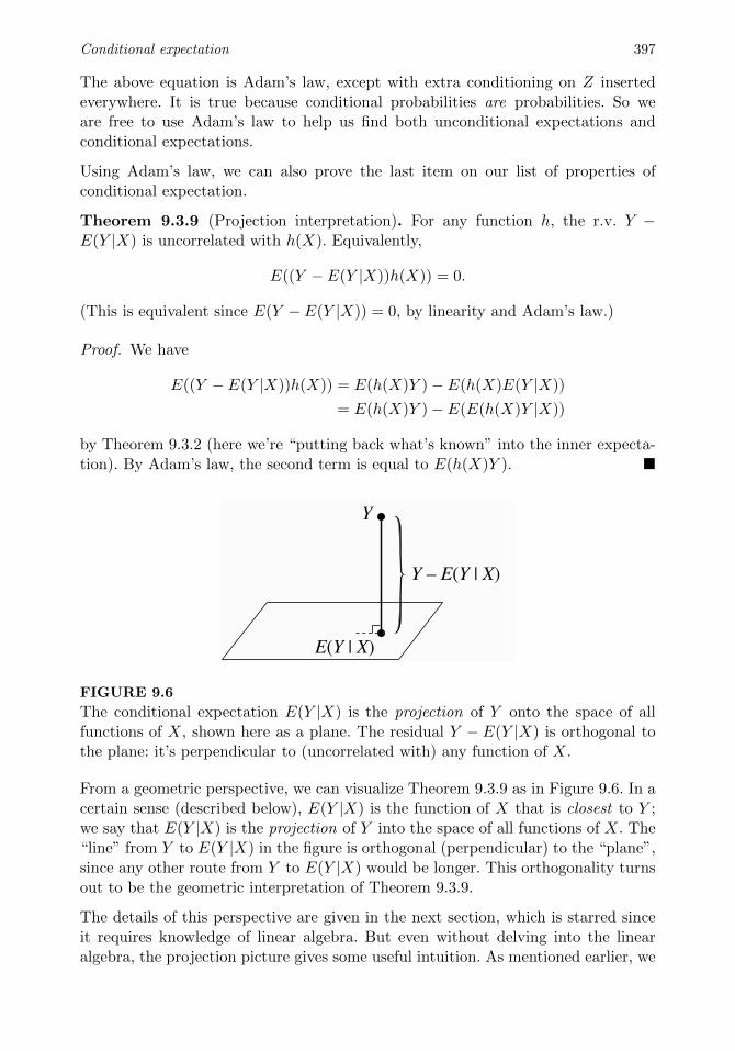
Theorem 9.3.9 (Projection interpretation). For any function h, the r.v. Y �E(Y |X) is uncorrelated with h(X). Equivalently,

E((Y � E(Y |X))h(X)) = 0.

(This is equivalent since E(Y � E(Y |X)) = 0, by linearity and Adam’s law.)

Proof. We have

E((Y � E(Y |X))h(X)) = E(h(X)Y ) � E(h(X)E(Y |X))

= E(h(X)Y ) � E(E(h(X)Y |X))

by Theorem 9.3.2 (here we’re “putting back what’s known” into the inner expecta-tion). By Adam’s law, the second term is equal to E(h(X)Y ). ⌅

Y

E(Y | X)

Y – E(Y | X)

FIGURE 9.6

The conditional expectation E(Y |X) is the projection of Y onto the space of allfunctions of X, shown here as a plane. The residual Y � E(Y |X) is orthogonal tothe plane: it’s perpendicular to (uncorrelated with) any function of X.

From a geometric perspective, we can visualize Theorem 9.3.9 as in Figure 9.6. In acertain sense (described below), E(Y |X) is the function of X that is closest to Y ;we say that E(Y |X) is the projection of Y into the space of all functions of X. The“line” from Y to E(Y |X) in the figure is orthogonal (perpendicular) to the “plane”,since any other route from Y to E(Y |X) would be longer. This orthogonality turnsout to be the geometric interpretation of Theorem 9.3.9.

The details of this perspective are given in the next section, which is starred sinceit requires knowledge of linear algebra. But even without delving into the linearalgebra, the projection picture gives some useful intuition. As mentioned earlier, we


can think of E(Y |X) as a prediction for Y based on X. This is an extremely com-mon problem in statistics: predict or estimate the future observations or unknownparameters based on data. The projection interpretation of conditional expectationimplies that E(Y |X) is the best predictor of Y based on X, in the sense that it isthe function of X with the lowest mean squared error (expected squared di↵erencebetween Y and the prediction of Y ).

Example 9.3.10 (Linear regression). An extremely widely used method for dataanalysis in statistics is linear regression. In its most basic form, the linear regressionmodel uses a single explanatory variable X to predict a response variable Y , and itassumes that the conditional expectation of Y is linear in X:

E(Y |X) = a + bX.

(a) Show that an equivalent way to express this is to write

Y = a + bX + ✏,

where ✏ is an r.v. (called the error) with E(✏|X) = 0.

(b) Solve for the constants a and b in terms of E(X), E(Y ), Cov(X, Y ), and Var(X).

Solution:

(a) Let Y = a + bX + ✏, with E(✏|X) = 0. Then by linearity,

E(Y |X) = E(a|X) + E(bX|X) + E(✏|X) = a + bX.

Conversely, suppose that E(Y |X) = a + bX, and define

✏ = Y � (a + bX).

Then Y = a + bX + ✏, with

E(✏|X) = E(Y |X) � E(a + bX|X) = E(Y |X) � (a + bX) = 0.

(b) First, by Adam’s law, taking the expectation of both sides gives

E(Y ) = a + bE(X).

Note that ✏ has mean 0 and X and ✏ are uncorrelated, since

E(✏) = E(E(✏|X)) = E(0) = 0

andE(✏X) = E(E(✏X|X)) = E(XE(✏|X)) = E(0) = 0.

Taking the covariance with X of both sides in Y = a + bX + ✏, we have

Cov(X, Y ) = Cov(X, a) + bCov(X, X) + Cov(X, ✏) = bVar(X).


Thus,

b =Cov(X, Y )

Var(X),

a = E(Y ) � bE(X) = E(Y ) � Cov(X, Y )

Var(X)· E(X).

⇤

9.4 *Geometric interpretation of conditional expectation

This section explains in more detail the geometric perspective shown in Figure 9.6,using some concepts from linear algebra. Consider the vector space consisting of allrandom variables on a certain probability space, such that the random variables eachhave zero mean and finite variance. (To apply the concepts of this section to r.v.sthat don’t have zero mean, we can center them first by subtracting their means.)Each vector or point in the space is a random variable (here we are using “vector”in the linear algebra sense, not in the sense of a random vector from Chapter 7).Define the inner product of two r.v.s U and V to be

hU, V i = Cov(U, V ) = E(UV ).

(For this definition to satisfy the axioms for an inner product, we need the conventionthat two r.v.s are considered the same if they are equal with probability 1.)

With this definition, two r.v.s are uncorrelated if and only if they have an innerproduct of 0, which means they are orthogonal in the vector space. The squaredlength of an r.v. X is

||X||2 = hX, Xi = Var(X) = EX2,

so the length of an r.v. is its standard deviation. The squared distance betweentwo r.v.s U and V is E(U � V )2, and the cosine of the angle between them is thecorrelation between them.

The random variables that can be expressed as functions of X form a subspace ofthe vector space. In Figure 9.6, the subspace of random variables of the form h(X)is represented by a plane. To get E(Y |X), we project Y onto the plane. Then theresidual Y � E(Y |X) is orthogonal to h(X) for all functions h, and E(Y |X) is thefunction of X that best predicts Y , where “best” here means that the mean squarederror E(Y � g(X))2 is minimized by choosing g(X) = E(Y |X).

The projection interpretation is a helpful way to think about many of the propertiesof conditional expectation. For example, if Y = h(X) is a function of X, then Y itself


is already in the “plane”, so it is its own projection; this explains why E(h(X)|X) =h(X). Also, we can think of unconditional expectation as a projection too: E(Y ) =E(Y |0) is the projection of Y onto the space of all constants (and indeed, E(Y ) isthe constant c that minimizes E(Y � c)2, as we proved in Theorem 6.1.4).

We can now also give a geometric interpretation for Adam’s law: E(Y ) says toproject Y in one step to the space of all constants; E(E(Y |X)) says to do it in twosteps, by first projecting onto the “plane” and then projecting E(Y |X) onto thespace of all constants, which is a line within that “plane”. Adam’s law says that theone-step and two-step methods yield the same result.

9.5 Conditional variance

Once we’ve defined conditional expectation given an r.v., we have a natural way todefine conditional variance given an r.v.: replace all instances of E(·) in the definitionof unconditional variance with E(·|X).

Definition 9.5.1 (Conditional variance). The conditional variance of Y given X

is

Var(Y |X) = E((Y � E(Y |X))2|X).

This is equivalent to

Var(Y |X) = E(Y 2|X) � (E(Y |X))2.

h 9.5.2. Like E(Y |X), Var(Y |X) is a random variable, and it is a function of X.

Since conditional variance is defined in terms of conditional expectations, we canuse results about conditional expectation to help us calculate conditional variance.Here’s an example.

Example 9.5.3. Let Z ⇠ N (0, 1) and Y = Z2. Find Var(Y |Z) and Var(Z|Y ).

Solution:

Without any calculations we can see that Var(Y |Z) = 0: conditional on Z, Y isa known constant, and the variance of a constant is 0. By the same reasoning,Var(h(Z)|Z) = 0 for any function h.

To get Var(Z|Y ), apply the definition:

Var(Z|Z2) = E(Z2|Z2) � (E(Z|Z2))2.

The first term equals Z2. The second term equals 0 by symmetry, as we found in

Example 9.3.3. Thus Var(Z|Z2) = Z2, which we can write as Var(Z|Y ) = Y . ⇤


We learned in the previous section that Adam’s law relates conditional expectationto unconditional expectation. A companion result for Adam’s law is Eve’s law, whichrelates conditional variance to unconditional variance.

Theorem 9.5.4 (Eve’s law). For any r.v.s X and Y ,

Var(Y ) = E(Var(Y |X)) + Var(E(Y |X)).

The ordering of E’s and Var’s on the right-hand side spells EVVE, whence thename Eve’s law. Eve’s law is also known as the law of total variance or the variancedecomposition formula.

Proof. Let g(X) = E(Y |X). By Adam’s law, E(g(X)) = E(Y ). Then

E(Var(Y |X)) = E(E(Y 2|X) � g(X)2) = E(Y 2) � E(g(X)2),

Var(E(Y |X)) = E(g(X)2) � (Eg(X))2 = E(g(X)2) � (EY )2.

Adding these equations, we have Eve’s law. ⌅

To visualize Eve’s law, imagine a population where each person has a value of X

and a value of Y . We can divide this population into subpopulations, one for eachpossible value of X. For example, if X represents age and Y represents height, wecan group people based on age. Then there are two sources contributing to thevariation in people’s heights in the overall population. First, within each age group,people have di↵erent heights. The average amount of variation in height within eachage group is the within-group variation, E(Var(Y |X)). Second, across age groups,the average heights are di↵erent. The variance of average heights across age groupsis the between-group variation, Var(E(Y |X)). Eve’s law says that to get the totalvariance of Y , we simply add these two sources of variation.

Figure 9.7 illustrates Eve’s law in the simple case where we have three age groups.The average amount of scatter within each of the groups X = 1, X = 2, andX = 3 is the within-group variation, E(Var(Y |X)). The variance of the groupmeans E(Y |X = 1), E(Y |X = 2), and E(Y |X = 3) is the between-group variation,Var(E(Y |X)).

X = 1 X = 2 X = 3

FIGURE 9.7

Eve’s law says that total variance is the sum of within-group and between-groupvariation.


Another way to think about Eve’s law is in terms of prediction. If we wanted topredict someone’s height based on their age alone, the ideal scenario would be if ev-eryone within an age group had exactly the same height, while di↵erent age groupshad di↵erent heights. Then, given someone’s age, we would be able to predict theirheight perfectly. In other words, the ideal scenario for prediction is no within-groupvariation in height, since the within-group variation cannot be explained by age dif-ferences. For this reason, within-group variation is also called unexplained variation,and between-group variation is also called explained variation. Eve’s law says thatthe total variance of Y is the sum of unexplained and explained variation.

h 9.5.5. Let Y be an r.v. and A be an event. It is wrong to say “Var(Y ) =Var(Y |A)P (A) + Var(Y |Ac)P (Ac)”, even though this looks analogous to the lawof total expectation. Rather, we should use Eve’s law if we want to condition onwhether or not A occurred: letting I be the indicator of A,

Var(Y ) = E(Var(Y |I)) + Var(E(Y |I)).

To see how this expression relates to the “wrong expression”, let

p = P (A), q = P (Ac), a = E(Y |A), b = E(Y |Ac), v = Var(Y |A), w = Var(Y |Ac).

Then E(Y |I) is a with probability p and b with probability q, and Var(Y |I) is v

with probability p and w with probability q. So

E(Var(Y |I)) = vp + wq = Var(Y |A)P (A) + Var(Y |Ac)P (Ac),

which is exactly the “wrong expression”, and Var(Y ) consists of this plus the term

Var(E(Y |I)) = a2p + b

2q � (ap + bq)2.

It is crucial to account for both within-group and between-group variation.

9.6 Adam and Eve examples

We conclude this chapter with several examples showing how Adam’s law and Eve’slaw allow us to find the mean and variance of complicated r.v.s, especially in situ-ations that involve multiple levels of randomness.

In our first example, the r.v. of interest is the sum of a random number of randomvariables. There are thus two levels of randomness: first, each term in the sumis a random variable; second, the number of terms in the sum is also a randomvariable.

Example 9.6.1 (Random sum). A store receives N customers in a day, where N

is an r.v. with finite mean and variance. Let Xj be the amount spent by the jth


customer at the store. Assume that each Xj has mean µ and variance �2, and that

N and all the Xj are independent of one another. Find the mean and variance of

the random sum X =P

N

j=1 Xj , which is the store’s total revenue in a day, in terms

of µ, �2, E(N), and Var(N).

Solution:

Since X is a sum, our first impulse might be to claim “E(X) = Nµ by linearity”.Alas, this would be a category error, since E(X) is a number and Nµ is a randomvariable. The key is that X is not merely a sum, but a random sum; the number ofterms we are adding up is itself random, whereas linearity applies to sums with afixed number of terms.

Yet this category error actually suggests the correct strategy: if only we were allowedto treat N as a constant, then linearity would apply. So let’s condition on N ! Bylinearity of conditional expectation,

E(X|N) = E(NX

j=1

Xj |N) =NX

j=1

E(Xj |N) =NX

j=1

E(Xj) = Nµ.

We used the independence of the Xj and N to assert E(Xj |N) = E(Xj) for allj. Note that the statement “E(X|N) = Nµ” is not a category error because bothsides of the equality are r.v.s that are functions of N . Finally, by Adam’s law,

E(X) = E(E(X|N)) = E(Nµ) = µE(N).

This is a pleasing result: the average total revenue is the average amount spent percustomer, multiplied by the average number of customers.

For Var(X), we again condition on N to get Var(X|N):

Var(X|N) = Var(NX

j=1

Xj |N) =NX

j=1

Var(Xj |N) =NX

j=1

Var(Xj) = N�2.

Eve’s law then tells us how to obtain the unconditional variance of X:

Var(X) = E(Var(X|N)) + Var(E(X|N))

= E(N�2) + Var(Nµ)

= �2E(N) + µ

2Var(N).

⇤

In the next example, two levels of randomness arise because our experiment takesplace in two stages. We sample a city from a group of cities, then sample citizenswithin the city. This is an example of a multilevel model.


Example 9.6.2 (Random sample from a random city). To study the prevalenceof a disease in several cities of interest within a certain county, we pick a city atrandom, then pick a random sample of n people from that city. This is a form of awidely used survey technique known as cluster sampling.

Let Q be the proportion of diseased people in the chosen city, and let X be thenumber of diseased people in the sample. As illustrated in Figure 9.8 (where whitedots represent healthy individuals and black dots represent diseased individuals),di↵erent cities may have very di↵erent prevalences. Since each city has its owndisease prevalence, Q is a random variable. Suppose that Q ⇠ Unif(0, 1). Alsoassume that conditional on Q, each individual in the sample independently hasprobability Q of having the disease; this is true if we sample with replacement fromthe chosen city, and is approximately true if we sample without replacement butthe population size is large. Find E(X) and Var(X).

FIGURE 9.8

A certain oval-shaped county has 4 cities. Each city has healthy people (representedas white dots) and diseased people (represented as black dots). A random city ischosen, and then a random sample of n people is chosen from within that city.There are two components to the variability in the number of diseased people inthe sample: variation due to di↵erent cities having di↵erent disease prevalence, andvariation due to the randomness of the sample within the chosen city.

Solution:

With our assumptions, X|Q ⇠ Bin(n, Q); this notation says that conditional onknowing the disease prevalence in the chosen city, we can treat Q as a constant,and each sampled individual is an independent Bernoulli trial with probability Q ofsuccess. Using the mean and variance of the Binomial distribution, E(X|Q) = nQ

and Var(X|Q) = nQ(1 � Q). Furthermore, using the moments of the standardUniform distribution, E(Q) = 1/2, E(Q2) = 1/3, and Var(Q) = 1/12. Now we canapply Adam’s law and Eve’s law to get the unconditional mean and variance of X:

E(X) = E(E(X|Q)) = E(nQ) =n

2,


Var(X) = E(Var(X|Q)) + Var(E(X|Q))

= E(nQ(1 � Q)) + Var(nQ)

= nE(Q) � nE(Q2) + n2Var(Q)

=n

6+

n2

12.

Note that the structure of this problem is identical to that in the story of Bayes’billiards. Therefore, we actually know the distribution of X, not just its mean andvariance: X is Discrete Uniform on {0, 1, 2, . . . , n}. But the Adam-and-Eve approachcan be applied when Q has a more complicated distribution, or with more levels inthe multilevel model, whether or not it is feasible to work out the distribution ofX. For example, we could have people within cities within counties within stateswithin countries. ⇤Last but not least, we revisit Story 8.4.5, the Gamma-Poisson problem from theprevious chapter.

Example 9.6.3 (Gamma-Poisson revisited). Recall that Fred decided to find outabout the rate of Blotchville’s Poisson process of buses by waiting at the bus stopfor t hours and counting the number of buses Y . He then used the data to updatehis prior distribution � ⇠ Gamma(r0, b0). Thus, Fred was using the two-level model

� ⇠ Gamma(r0, b0)

Y |� ⇠ Pois(�t).

We found that under Fred’s model, the marginal distribution of Y is NegativeBinomial with parameters r = r0 and p = b0/(b0 + t). By the mean and variance ofthe Negative Binomial distribution, we have

E(Y ) =rq

p=

r0t

b0,

Var(Y ) =rq

p2=

r0t(b0 + t)

b20

.

Let’s independently verify this with Adam’s law and Eve’s law. Using resultsabout the Poisson distribution, the conditional mean and variance of Y given �

are E(Y |�) = Var(Y |�) = �t. Using results about the Gamma distribution, themarginal mean and variance of � are E(�) = r0/b0 and Var(�) = r0/b

20. For Adam

and Eve, this is all that is required:

E(Y ) = E(E(Y |�)) = E(�t) =r0t

b0,

Var(Y ) = E(Var(Y |�)) + Var(E(Y |�))

= E(�t) + Var(�t)

=r0t

b0+

r0t2

b20

=r0t(b0 + t)

b20

,


which is consistent with our earlier answers. The di↵erence is that when using Adamand Eve, we don’t need to know that Y is Negative Binomial! If we had been toolazy to derive the marginal distribution of Y , or if we weren’t so lucky as to have anamed distribution for Y , Adam and Eve would still deliver the mean and varianceof Y (though not the PMF).

Lastly, let’s compare the mean and variance of Y under the two-level model tothe mean and variance we would get if Fred were absolutely sure of the true valueof �. In other words, suppose we replaced � by its mean, E(�) = r0/b0, making� a constant instead of an r.v. Then the marginal distribution of the number ofbuses (which we’ll call Y under the new assumptions) would just be Poisson withparameter r0t/b0. Then we would have

E(Y ) =r0t

b0,

Var(Y ) =r0t

b0.

Notice that E(Y ) = E(Y ), but Var(Y ) < Var(Y ): the extra term r0t2/b

20 from Eve’s

law is missing. Intuitively, when we fix � at its mean, we are eliminating a level ofuncertainty in the model, and this causes a reduction in the unconditional variance.

Figure 9.9 overlays the plots of two PMFs, that of Y ⇠ NBin(r0, b0/(b0 + t)) in grayand that of Y ⇠ Pois(r0t/b0) in black. The values of the parameters are arbitrarilychosen to be r0 = 5, b0 = 1, t = 2. These two PMFs have the same center of mass,but the PMF of Y is noticeably more dispersed.

0 5 10 15 20

0.00

0.05

0.10

0.15

0.20

x

PMF

● ● ●●

●

●

●

●

●

● ●

●

●

●

●

●

●●

● ● ●●

●

●

●

●

●●

● ● ●●

●●

●●

●●

●●

● ●

FIGURE 9.9

PMF of Y ⇠ NBin(r0, b0/(b0 + t)) in gray and Y ⇠ Pois(r0t/b0) in black, wherer0 = 5, b0 = 1, t = 2.

⇤


9.7 Recap

To calculate an unconditional expectation, we can divide up the sample space anduse the law of total expectation

E(Y ) =nX

i=1

E(Y |Ai)P (Ai),

but we must be careful not to destroy information in subsequent steps (such as byforgetting in the midst of a long calculation to condition on something that needs tobe conditioned on). In problems with a recursive structure, we can also use first-stepanalysis for expectations.

The conditional expectation E(Y |X) and conditional variance Var(Y |X) are ran-dom variables that are functions of X; they are obtained by treating X as if itwere a known constant. If X and Y are independent, then E(Y |X) = E(Y ) andVar(Y |X) = Var(Y ). Conditional expectation has the properties

E(h(X)Y |X) = h(X)E(Y |X)

E(Y1 + Y2|X) = E(Y1|X) + E(Y2|X),

analogous to the properties E(cY ) = cE(Y ) and E(Y1 + Y2) = E(Y1) + E(Y2) forunconditional expectation. The conditional expectation E(Y |X) is also the randomvariable that makes the residual Y � E(Y |X) uncorrelated with any function of X,which means we can interpret it geometrically as a projection.

Finally, Adam’s law and Eve’s law,

E(Y ) = E(E(Y |X))

Var(Y ) = E(Var(Y |X)) + Var(E(Y |X)),

often help us calculate E(Y ) and Var(Y ) in problems that feature multiple formsor levels of randomness.

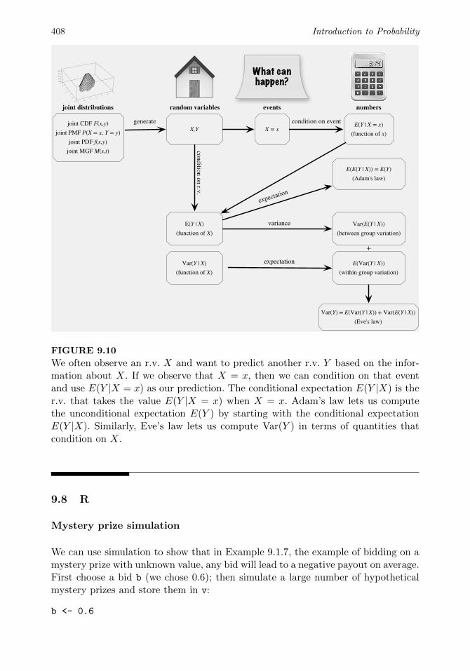
Figure 9.10 illustrates how the number E(Y |X = x) connects with the r.v. E(Y |X),whose expectation is E(Y ) by Adam’s law. Additionally, it shows how the ingredi-ents in Eve’s law are formed and come together to give a useful decomposition ofVar(Y ) in terms of quantities that condition on X.


X,YE(Y | X = x)

(function of x)

condition on r.v.

random variables events numbers

X = xgenerate

Var(Y) = E(Var(Y | X)) + Var(E(Y | X))(Eve's law)

E(Y | X)(function of X)

E(E(Y | X)) = E(Y) (Adam's law)

x

−3−2

−10

12

3y

−3

−2

−1

0

1

2

3

0.00

0.05

0.10

0.15

0.20

joint CDF F(x,y)joint PMF P(X = x, Y = y)

joint PDF f(x,y)joint MGF M(s,t)

joint distributions

Var(Y | X)(function of X)

condition on event

E(Var(Y | X))(within group variation)

Var(E(Y | X))(between group variation)

+

variance

expectation

expectation

What can happen?

FIGURE 9.10

We often observe an r.v. X and want to predict another r.v. Y based on the infor-mation about X. If we observe that X = x, then we can condition on that eventand use E(Y |X = x) as our prediction. The conditional expectation E(Y |X) is ther.v. that takes the value E(Y |X = x) when X = x. Adam’s law lets us computethe unconditional expectation E(Y ) by starting with the conditional expectationE(Y |X). Similarly, Eve’s law lets us compute Var(Y ) in terms of quantities thatcondition on X.

9.8 R

Mystery prize simulation

We can use simulation to show that in Example 9.1.7, the example of bidding on amystery prize with unknown value, any bid will lead to a negative payout on average.First choose a bid b (we chose 0.6); then simulate a large number of hypotheticalmystery prizes and store them in v:

b <- 0.6


nsim <- 10^5

v <- runif(nsim)

The bid is accepted if b > (2/3)*v. To get the average profit conditional on anaccepted bid, we use square brackets to keep only those values of v satisfying thecondition:

mean(v[b > (2/3)*v]) - b

This value is negative regardless of b, as you can check by experimenting withdi↵erent values of b.

Time until HH vs. HT

To verify the results of Example 9.1.9, we can start by generating a long sequenceof fair coin tosses. This is done with the sample command. We use paste with thecollapse="" argument to turn these tosses into a single string of H’s and T ’s:

paste(sample(c("H","T"),100,replace=TRUE),collapse="")

A sequence of length 100 is enough to virtually guarantee that both HH and HTwill have appeared at least once.

To determine how many tosses are required on average to see HH and HT, weneed to generate many sequences of coin tosses. For this, we use our familiar friendreplicate:

r <- replicate(10^3,paste(sample(c("H","T"),100,replace=T),collapse=""))

Now r contains a thousand sequences of coin tosses, each of length 100. To find thefirst appearance of HH in each of these sequences, it is easiest to use the str_locatecommand, located in the stringr package. After you’ve installed and loaded thepackage,

t <- str_locate(r,"HH")

creates a two-column table t, whose columns contain the starting and ending posi-tions of the first appearance of HH in each sequence of coin tosses. (Use head(t) todisplay the first few rows of the table and get an idea of what your results look like.)What we want are the ending positions, given by the second column. In particular,we want the average value of the second column, which is an approximation of theaverage waiting time for HH :

mean(t[,2])

Is your answer around 6? Trying again with "HT" instead of "HH", is your answeraround 4?


Linear regression

In Example 9.3.10, we derived formulas for the slope and intercept of a linear regres-sion model, which can be used to predict a response variable using an explanatoryvariable. Let’s try to apply these formulas to a simulated dataset:

x <- rnorm(100)

y <- 3 + 5*x + rnorm(100)

The vector x contains 100 realizations of the random variable X ⇠ N (0, 1), and thevector y contains 100 realizations of the random variable Y = a + bX + ✏ where✏ ⇠ N (0, 1). As we can see, the true values of a and b for this dataset are 3 and 5,respectively. We can visualize the data as a scatterplot with plot(x,y).

Now let’s see if we can get good estimates of the true a and b, using the formulasin Example 9.3.10:

b <- cov(x,y) / var(x)

a <- mean(y) - b*mean(x)

Here cov(x,y), var(x), and mean(x) provide the sample covariance, sample vari-ance, and sample mean, estimating the quantities Cov(X, Y ), Var(X), and E(X),respectively. (We have discussed sample mean and sample variance in detail in ear-lier chapters. Sample covariance is defined analogously, and is a natural way toestimate the true covariance.)

You should find that b is close to 5 and a is close to 3. These estimated values definethe line of best fit. The abline command lets us plot the line of best fit on top ofour scatterplot:

plot(x,y)

abline(a=a,b=b)

The first argument to abline is the intercept of the line, and the second argumentis the slope.

9.9 Exercises

Conditional expectation given an event

1. Fred wants to travel from Blotchville to Blissville, and is deciding between 3 options(involving di↵erent routes or di↵erent forms of transportation). The jth option wouldtake an average of µj hours, with a standard deviation of �j hours. Fred randomlychooses between the 3 options, with equal probabilities. Let T be how long it takes forhim to get from Blotchville to Blissville.

(a) Find E(T ). Is it simply (µ1 + µ2 + µ3)/3, the average of the expectations?

(b) Find Var(T ). Is it simply (�21 + �

22 + �

23)/3, the average of the variances?

introduction to probability - mcgill university

Documents