Introduction to Programming in R Introduction to the

R language,

CCCB course on R and Bioconductor, Dec 2011,

Aedin Culhane (My email is: aedin@jimmy.harvard.edu)

I Obtaining and managing R

R can be downloaded from the website: http://cran.r-project.org/. See additional notes whichgive a very detailed description on downloading and installing R (and Bioconductor).

R is available for all platforms: Unix/Linux, Windows and Mac. In this course, we will concentrateon the Windows implementation. The differences between the platforms are minor, so most of thematerial is applicable to the other platforms.

See the associated file on the course website, in which I give detailed instructions on downloadingand installing R and Bioconductor (for windows).

II The default R interface

This is the default user interface with the standard installation of R. In the course we will mostlyuse RStudio which provides a richer interface. RStudio can be obtained from www.rstudio.org)

� Start up R (go to the program Menu and find it in the Statistics folder)

� First, notice the different menus and icons in R. On the menu bar, there are the menus:

– File - load script, load/save session (workspace) or command history. Change Directory

– Edit - Cut/Paste. GUI preferences

– View

– Misc - stop computations, list/remove objects in session

– Packages - allows one to install new, update packages

– Windows

– Help - An essential resource!

� The icons below will allow one to

– open script (.R file),

– load image (previous R session, .RData file)

– save .R script

1

– copy and paste

– stop a computation (this can be an important button, but the ESC also works!)

– print.

II.1 Default R Editor

� Within R, one can open an editor using the menu command File -> New script

� Can type commands in the editor

� Highlight the commands and type Ctrl^R to submit the commands for R evaluation

� Evaluation of the commands can be stopped by pressing the Esc key or the Stop button

� Saving (Ctrl^S) and opening saved commands (Ctrl^O)

� Can open a new editor by typing Ctrl^N

II.2 Setting R default properties (on Windows)

The first thing to do when starting an R session, is to ensure that you will be able to find your dataand also that your output will be saved to a useful location on your computer hard-drive. Therefore,check the ”working directory”.

This maybe set by default to the depths of the operating system (C:/program files/R), which is apoor ”working” location. You may wish to change the default start location by right mouse clickingon the R icon on the desktop/start menu and changing the ”Start In” property. For example makea folder ’C:/work’, and make this as a ”Start in” folder. Alternatively you can change your workingdirectory, once you start R (see below)

III Starting out - Changing directory

The first thing to do when starting an R session, is to ensure that you will be able to find your dataand also that your output will be saved to a useful location on your computer hard-drive.

To change the default start location, right mouse click on the R icon on the (Windows) desktop/startmenu and changing the ”Start In” property. For example make a folder ’C:/work’, and make this asa ”Start in” folder. Alternatively you can change your working directory

When you start R, and see the prompt > , it may appear as if nothing is happening. This promptis now awaiting commands from you. This can be daunting to the new user, however it is easy tolearn a few commands and get started.

First, to change the directory after you have started R. Use the file menu, to change directory: File-> Change dir If you wish to type R commands to set or change working directories, use the following

> getwd()

2

To change the directory:

setwd("C:/work")

getwd()

I may create a new working directory for each R session which I call projectNameDate (eg colon-Jan13). If you have files in the working directory, you can see the contents of your working folderusing the functions/commands

> dir()

> dir(pattern = ".txt")

Within R Studio you can change and view the contents of a directory using the lower right panel.Click on the Files tab. To set a direct a working directory, navigate to the directory you wish toset as your home directory. To navigate up a directory, click on the triple dot icon on the top right.Once you are in the correct directory and see your data files, click on the More (blue cogwheel), andselect ”Set as Working Directory ”

IV R Packages

By default, R is packaged with a small number of essential packages, however as we saw there aremany contributed R packages.

1. Some packages are loaded by default with every R session. The libraries included in the Table?? are loaded on the R startup.

Table 1: Preloaded packagesPackage Description

base Base R functionsdatasets Base R datasetsgrDevices Graphics devices for base and grid graphicsgraphics R functions for base graphicsmethods Formally defined methods and classes for R objects,

plus other programming toolsstats R statistical functions.utils R utility functions

To see which packages are currently loaded, use

> search()

> sessionInfo()

To see which packages are installed on your computer, issue the command

3

> library()

Within RStudio installed packages can be view in the Package Tab of the lower right panel.

You will very likely want to install additional packages or libraries.

V R libraries

There are several thousand R packages and >500 Bioconductor packages (also called libraries)available. Not all of them, actually a small subset, will be useful to us. R users are free toselected which libraries to install. These are not installed by default, so we have to select andinstall additional packages that will be of use to us.

Sometimes I have problems installing R packages using RStudio. Until this is resolved (Dec2011), I recommend using the traditional R GUI or command line for installation of R packages.

In the R GUI You can install additional packages using the drop-down menu Packages (prob-ably the easiest route) or using the following commands

> install.packages("Design")

> update.packages("Design")

To use the drop-down menu. Click on “Packages”

� Go to “Set CRAN mirror” and choose an available mirror (choose one close by, it’ll befaster hopefully).

� If you know the name of the package you want to install, or if you want to install all theavailable packages, click on “Packages” again and choose “Install package(s) from CRAN”To select more than one page, use shift-mouse click or control-mouse click.

� Installation of all packages takes some time and space on your computer.

� If the name of the package is not known, you could use taskviews help or archives of themailing list to pinpoint one. Also look on the R website Task views description of packages(see Additional Notes in Installation which I have provided).

Once you have installed a package, you do NOT need to re-install it. But to load the libraryin your current R session use the commands

> library(Design)

> require(Design)

> sessionInfo()

> library()

> data()

You can unload the loaded package pkg by

> detach(package:Design)

> search()

To get an information on a package, type

4

> library(help = Design)

NOTE: Packages are often inter-dependent, and loading one may cause others to be automat-ically loaded.

VI Datasets in R

Both the R core installation and contributed R package contain datasets, which are useful exampledata when learning R. To list all available data sets:

> data()

To load a dataset, for example, the dataset women which gives the average heights and weights for15 American women aged 3039.

> data(women)

> ls()

> ls(pattern = "w")

VII Getting help with functions and features

There are many resources for help in R.

� Emmanuel Paradis has an excellent beginners guide to R available from http://cran.r-project.

org/doc/contrib/Paradis-rdebuts_en.pdf

� There is an introduction to R classes and objects on the R website http://cran.r-project.

org/doc/manuals/R-intro.html and also see Tom Guirkes manual at http://faculty.ucr.edu/~tgirke/Documents/R_BioCond/R_BioCondManual.html

� Tom Short’s provides a useful short R reference card at http://cran.r-project.org/doc/

contrib/Short-refcard.pdf

Within R, you can find help on any command (or find commands) using the follow:

� If you know the command (or part of it)

help(lm)

?matrix

apropos("mean")

example(rep)

5

The last command will run all the examples included with the help for a particular function.If we want to run particular examples, we can highlight the commands in the help window andsubmit them by typing Ctrl^V

� If you don’t know the command and want to do a keyword search for it.

> help.search("combination")

> help.start()

help.search will open a html web browser or a MSWindows help browser (depending on theyour preferences) in which you can browse and search R documentation.

� Finally, there is a large R community who are incredibly helpful. There is a mailing list for R,Bioconductor and almost every R project. It is useful to search the archives of these mailinglists. Frequently you will find someone encountered the same problem as you, and previouslyasked the R mailing list for help (and got a solution!).

� There are useful tools and resources on the web including:

– The R search engine http://www.Rseek.org

– R bloggers website http://www.r-bloggers.com/

VIII Interactive use of the R Editor

Note on the command line, the default prompt starts with an '>' If the command is not completeon one line, the continuation prompt is ’+’

Type q() to quit the program

VIII.1 R as a big calculator

Type the following into an R session (or copy and paste from this document).

> 2 + 2

[1] 4

> 2 * 2

[1] 4

> 2 * 100/4

[1] 50

6

> 2 * 100/4 + 2

[1] 52

> 2 * 100/(4 + 2)

[1] 33.33333

> 2^10

[1] 1024

> log(2)

[1] 0.6931472

> tmpVal <- log(2)

> tmpVal

[1] 0.6931472

> exp(tmpVal)

[1] 2

> rnorm(5)

[1] 0.4704752 0.7223814 1.4299385 0.4329091 -1.3395984

Note you can recover previous commands using the up and down arrow keys. Indeed you can recoverthe previous expressions entered (default 25) into the R session using the function history.

rnorm generates 10 random numbers from a normal distribution. Type this a few times (hint: theup arrow key is useful).

Note even in the simple use of R as a calculator, it is useful to store intermediate results, (tmpVal=log(2)).In this case, we assigned a symbolic variable tmpVal. Note when you assign a value to such a variable,there is no immediate visible result. We need to print(tmpVal) or just type tmpVal in order to seewhat value was assigned to tmpVal

7

IX Basic operators

IX.1 Comparison operators

� equal: ==

� not equal: !=

� greater/less than: > <

� greater/less than or equal: >= <=

> 1 == 1

[1] TRUE

IX.2 Logical operators

� AND & Returns TRUE if both comparisons return TRUE.

> x <- 1:10

> y <- 10:1

> x > y & x > 5

[1] FALSE FALSE FALSE FALSE FALSE TRUE TRUE TRUE TRUE TRUE

� OR | Returns TRUE where at least one comparison returns TRUE.

> x == y | x != y

[1] TRUE TRUE TRUE TRUE TRUE TRUE TRUE TRUE TRUE TRUE

� NOT ! The ’ !’ sign returns the negation (opposite) of a logical vector.

> !x > y

[1] TRUE TRUE TRUE TRUE TRUE FALSE FALSE FALSE FALSE FALSE

X A few important points on R

� R is case sensitive, i.e. myData and Mydata are different names

� Elementary commands: expressions are evaluated, printed and value lost; assignments evaluateexpressions, passes value to a variable, but not automatically printed

> 2 * 5^2

[1] 50

8

> x <- 2 * 5^2

> print(x)

[1] 50

� Assignment operators are: '<-', '=', '->'

> 2 * 5^2

[1] 50

> y <- 2 * 5^2

> z <- 2 * 5^2

> z <- 2 * 5^2

> print(y)

[1] 50

> x == y

[1] TRUE

> y == z

[1] TRUE

� '<-' is the most popular assignment operator, and '=' is a recent addition.

There is no space between < and −It is '<-' (less than and a minus symbol)

Although, unlikely, you may also see old code using '_', these is NOT used any more in R.

When assigning a value spaces are ignored so 'z<-3' is equivalent to 'z <- 3'

� Arguments (parameters) to a function calls f(x), PROC are enclosed in round brackets. Evenif no arguments are passed to a function, the round brackets are required.

print(x)

getwd()

� Comments can be put anywhere. To comment text, insert a hashmark #. Everything followingit to end of the line is commented out (ignored, not evaluated).

print(y) # Here is a comment

� Note on brackets. It is very important to use the correct brackets.

� ’==’ and ’=’ have very different uses in R. == is a binary operator, which test for equality(A==B determines if A ’is equal to’ B ).

� Quotes, you can use both ” double or ’ single quotes, as long as they are matched.

9

Bracket Use

() To set priorities 3*(2+4). Function calls f(x)[] Indexing in vectors, matrices, data frames{} Creating new functions. Grouping commands {mean(x); var(x)}

[[]] Indexing of lists

� For names, normally all alphanumeric symbols are allowed plus '.' and '_' Start names witha character [Aa-Zz] not a numeric character [0-9]. Avoid using single characters or functionnames t, c, q, diff, mean

� Commands can be grouped together with braces ('{' and '}').

� Missing values called represented by NA

10

XI R Objects

� Everything (variable, functions etc) in R is an object

� Every object has a class

XI.1 Managing R Objects

R creates and manipulates objects: variables, matrices, strings, functions, etc. objects are stored byname during an R session.

During a R session, you may create many objects, if you wish to list the objects you have created inthe current session use the command

> objects()

> ls()

The collection of objects is called workspace.

If you wish to delete (remove) objects, issue the commands:

rm(x,y,z, junk)

ls()

where x, y, junk were the objects created during the session.

Note rm(list=ls()) will remove everything. Use with caution

XI.2 Types of R objects

Objects can be thought of as a container which holds data or a function. The most basic form of datais a single element, such as a single numeric or a character string. However one can’t do statistics onsingle numbers! Therefore there are many other objects in R.

� A vector is an ordered collection of numerical, character, complex or logical objects. Vectorsare collection of atomic (same data type) components or modes. For example

> vec1 <- 1:10

> vec2 <- LETTERS[1:10]

> vec3 <- vec2 == "D"

> vec3

[1] FALSE FALSE FALSE TRUE FALSE FALSE FALSE FALSE FALSE FALSE

In each case above, these vectors have 10 elements, and are of length=10.

11

� A matrix is a multidimensional collection of data entries of the same type. Matrices have twodimensions. It has rownames and colnames.

> mat1 <- matrix(vec1, ncol = 2, nrow = 5)

> print(mat1)

[,1] [,2]

[1,] 1 6

[2,] 2 7

[3,] 3 8

[4,] 4 9

[5,] 5 10

> dim(mat1)

[1] 5 2

> colnames(mat1) = c("A", "B")

> rownames(mat1) = paste("N", 1:5, sep = "")

> print(mat1)

A B

N1 1 6

N2 2 7

N3 3 8

N4 4 9

N5 5 10

� A list is an ordered collection of objects that can be of different modes (e.g. numeric vector,array, etc.).

> a <- 20

> newList1 <- list(a, vec1, mat1)

> print(newList1)

[[1]]

[1] 20

[[2]]

[1] 1 2 3 4 5 6 7 8 9 10

[[3]]

A B

N1 1 6

N2 2 7

N3 3 8

N4 4 9

N5 5 10

12

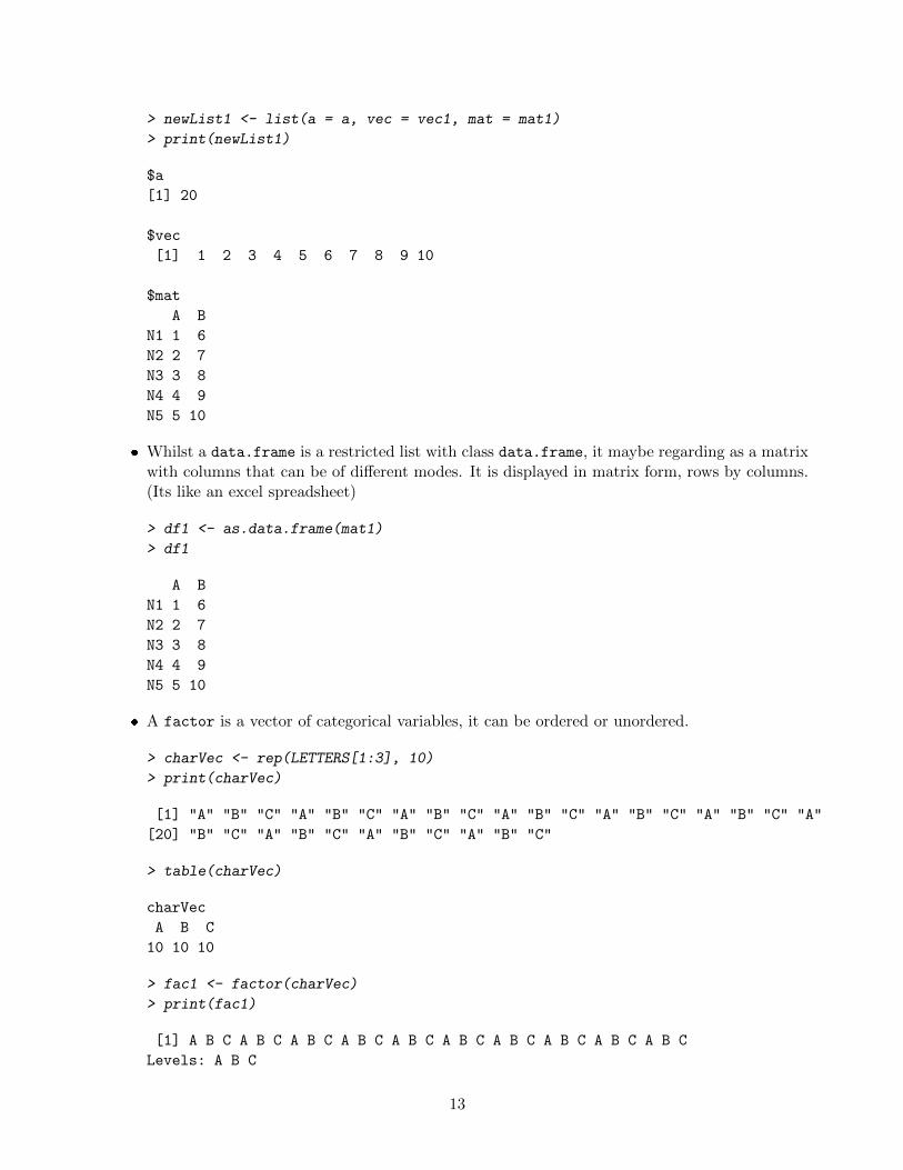
> newList1 <- list(a = a, vec = vec1, mat = mat1)

> print(newList1)

$a

[1] 20

$vec

[1] 1 2 3 4 5 6 7 8 9 10

$mat

A B

N1 1 6

N2 2 7

N3 3 8

N4 4 9

N5 5 10

� Whilst a data.frame is a restricted list with class data.frame, it maybe regarding as a matrixwith columns that can be of different modes. It is displayed in matrix form, rows by columns.(Its like an excel spreadsheet)

> df1 <- as.data.frame(mat1)

> df1

A B

N1 1 6

N2 2 7

N3 3 8

N4 4 9

N5 5 10

� A factor is a vector of categorical variables, it can be ordered or unordered.

> charVec <- rep(LETTERS[1:3], 10)

> print(charVec)

[1] "A" "B" "C" "A" "B" "C" "A" "B" "C" "A" "B" "C" "A" "B" "C" "A" "B" "C" "A"

[20] "B" "C" "A" "B" "C" "A" "B" "C" "A" "B" "C"

> table(charVec)

charVec

A B C

10 10 10

> fac1 <- factor(charVec)

> print(fac1)

[1] A B C A B C A B C A B C A B C A B C A B C A B C A B C A B C

Levels: A B C

13

> attributes(fac1)

$levels

[1] "A" "B" "C"

$class

[1] "factor"

> levels(fac1)

[1] "A" "B" "C"

� array An array in R can have one, two or more dimensions. I find it useful to store multiplerelated data.frame (for example when I jack-knife or permute data). Note if there are insufficientobjects to fill the array, R recycles (see below)

> array(1:24, dim = c(2, 4, 3))

, , 1

[,1] [,2] [,3] [,4]

[1,] 1 3 5 7

[2,] 2 4 6 8

, , 2

[,1] [,2] [,3] [,4]

[1,] 9 11 13 15

[2,] 10 12 14 16

, , 3

[,1] [,2] [,3] [,4]

[1,] 17 19 21 23

[2,] 18 20 22 24

> array(1:23, dim = c(2, 4, 3))

, , 1

[,1] [,2] [,3] [,4]

[1,] 1 3 5 7

[2,] 2 4 6 8

, , 2

[,1] [,2] [,3] [,4]

[1,] 9 11 13 15

[2,] 10 12 14 16

14

, , 3

[,1] [,2] [,3] [,4]

[1,] 17 19 21 23

[2,] 18 20 22 1

> array(1:23, dim = c(2, 4, 3), dimnames = list(paste("Patient",

+ 1:2, sep = ""), LETTERS[1:4], c("X", "Y", "Z")))

, , X

A B C D

Patient1 1 3 5 7

Patient2 2 4 6 8

, , Y

A B C D

Patient1 9 11 13 15

Patient2 10 12 14 16

, , Z

A B C D

Patient1 17 19 21 23

Patient2 18 20 22 1

XI.3 Attributes of R Objects

1. Basic attributes

The most basic and fundamental properties of every objects is its mode and length. Theseare intrinsic attributes of every object. Examples of mode are ”logical”, ”numeric”, ”character”,”list”, ”expression”, ”name/symbol” and ”function”.

Of which the most basic of these are:

� 'character': a character string

� 'numeric': a real number, which can be an integer or a double

� 'integer': an integer

� 'logical': a logical (true/false) value

> x <- 3

> mode(x)

[1] "numeric"

15

> x <- "apple"

> mode(x)

[1] "character"

> x <- 3.145

> x + 2

[1] 5.145

> x == 2

[1] FALSE

> x <- x == 2

> x

[1] FALSE

> mode(x)

[1] "logical"

> x <- 1:10

> mode(x)

[1] "numeric"

> x <- LETTERS[1:5]

> mode(x)

[1] "character"

> x <- matrix(rnorm(50), nrow = 5, ncol = 10)

> mode(x)

[1] "numeric"

Repeat above, and find the length and class of x in each case.

2. Other attributes, dimension

> x <- matrix(5:14, nrow = 2, ncol = 5)

> x

[,1] [,2] [,3] [,4] [,5]

[1,] 5 7 9 11 13

[2,] 6 8 10 12 14

> attributes(x)

16

$dim

[1] 2 5

In summary

Object Modes Allow >1 Modes*

vector numeric, character, complex or logical No

matrix numeric, character, complex or logical No

list numeric, character, complex, logical, function, expression, ... Yes

data frame numeric, character, complex or logical Yes

factor numeric or character No

array numeric, character, complex or logical No*Whether object allows elements of different modes. For example all elements in a vector or array have

to be of the same mode. Whereas a list can contain any type of object including a list.

XI.4 Creating and accessing objects

We have already created a few objects: x, y, junk. Will create a few more and will select, accessand modify subsets of them.

� Create vectors, matrices and data frames using seq, rbind and cbind

> x.vec <- seq(1, 7, by = 2)

> names(x.vec) <- letters[1:4]

> xMat <- cbind(x.vec, rnorm(4), rep(5, 4))

> yMat <- rbind(1:3, rep(1, 3))

> z.mat <- rbind(xMat, yMat)

> x.df <- as.data.frame(xMat)

> names(x.df) <- c("ind", "random", "score")

� Accessing elements

> x.vec[1]

a

1

> x.vec["a"]

a

1

> xMat[2, 3]

[1] 5

> xMat[, c(2:3)]

17

a 0.5579345 5

b -0.7423902 5

c -0.6047593 5

d 0.4153831 5

> xMat[, -c(1)]

a 0.5579345 5

b -0.7423902 5

c -0.6047593 5

d 0.4153831 5

> xMat[xMat[, 1] > 3, ]

x.vec

c 5 -0.6047593 5

d 7 0.4153831 5

> x.df$ind

[1] 1 3 5 7

> x.df[, 1]

[1] 1 3 5 7

XI.5 Modifying elements

> xMat[3, 1] <- 6

> z.mat[, 2] <- 0

XI.6 Sorting and Ordering items

Sorting, might want to re-order the rows of a matrix or see the sorted elements of a vector

> z.vec <- c(5, 3, 8, 2, 3.2)

> sort(z.vec)

[1] 2.0 3.0 3.2 5.0 8.0

> order(z.vec)

[1] 4 2 5 1 3

18

> `?`(ChickWeight)

> ChickWeight[1:2, ]

weight Time Chick Diet

1 42 0 1 1

2 51 2 1 1

> chick.short <- ChickWeight[1:36, ]

> chick.srt <- chick.short[order(chick.short$Time, chick.short$weight),

+ ]

> chick.srt[1:2, ]

weight Time Chick Diet

13 40 0 2 1

1 42 0 1 1

> chickOrd <- chick.short[order(chick.short$weight), ]

19

XI.7 Missing Values

Missing values are assigned special value of ’NA’

> z <- c(1:3, NA)

> z

[1] 1 2 3 NA

> ind <- is.na(z)

> ind

[1] FALSE FALSE FALSE TRUE

To remove missing values from a vector

> print(z)

[1] 1 2 3 NA

> x <- z[!is.na(z)]

> print(x)

[1] 1 2 3

XI.8 Creating empty vectors and matrices

To create a empty vector, matrix or data.frame

> x1 <- numeric()

> x2 <- numeric(5)

> x1.mat <- matrix(0, nrow = 10, ncol = 3)

20

XII Reading and Writing Data in R

So far, we have only analyzed data that were already stored in R. Usually, we will work with our owndata and write the results of the data analysis in external files.

Basic tools for reading and writing data are respectively: read.table and write.table. We will go intofurther detail about each.

We will use the data from a study which examined the weight, height and age of women. Data fromthe women Study is available as an R dataset and information about this study can be found byusing R help (hint ?women).

Common data exchange formats are Excel, comma and tab-delimited format text files. Each of thesefiles will be provided on the course website. Or to create a tab-delimited and csv file, do the following:

1. Download the data set ”Women.xls” from the course website. Save it in your local directory.

2. Open this file ”Women.xls” in Excel.

3. To export data as comma or tab delimited text files. In Excel select File -> Save as andTab: select the format Text (Tab delimited) (*.txt).CSV: select the format CSV (Comma delimited) (*.csv).

XIII Importing and reading data into R

1. Using read.table()

(a) The most commonly used function for reading data is read.table(). It will read the datainto R as a data.frame.

By Default read.table() assumes a file is space delimited and it will fail if the file is in adifferent format with the error below.

Women<-read.table("Women.txt")

In order to read files that are tab or comma delimited, the defaults must be changed. Wealso need to specify that the table has a header row

> Women <- read.table("Women.txt", sep = "\t", header = TRUE)

> Women[1:2, ]

height weight age

1 58 115 33

2 59 117 34

> summary(Women)

height weight age

Min. :58.0 Min. :115.0 Min. :30.00

1st Qu.:61.5 1st Qu.:124.5 1st Qu.:32.00

Median :65.0 Median :135.0 Median :34.00

Mean :65.0 Mean :136.7 Mean :33.93

21

3rd Qu.:68.5 3rd Qu.:148.0 3rd Qu.:35.50

Max. :72.0 Max. :164.0 Max. :39.00

> class(Women$age)

[1] "integer"

Note by default, character vector (strings) are read in as factors. To turn this off, use theparameter as.is=TRUE

(b) Important options:

header==TRUE should be set to ’TRUE’, if your file contains the column names

as.is==TRUE otherwise the character columns will be read as factors

sep=”” field separator character (often comma ’,’ or tab ”�” eg: sep=”,”)

na.strings a vector of strings which are to be interpreted as ’NA’ values.

row.names The column which contains the row names

comment.char by default, this is the pound # symbol, use ”” to turn off interpretation of commented text.

> help(read.table)

Note the defaults for read.table(), read.csv(), read.delim() are different. For example,in read.table() function, we specify header=TRUE , as the first line is a line of headingsamong other parameters.

2. read.csv() is a derivative of read.table() which calls read.table() function with the followingoptions so it reads a comma separated file:

read.csv(file, header = TRUE, sep = ",", quote="\"", dec=".",

fill = TRUE, comment.char="", ...)

Read in a comma separated file:

> Women2 <- read.csv("Women.csv", header = TRUE)

> Women2[1:2, ]

height weight age

1 58 115 33

2 59 117 34

3. Reading directly from Website You can read a file directly from the web

> read.table("http://bcb.dfci.harvard.edu/~aedin/courses/Bioconductor/Women.txt",

+ header = TRUE)[1:2, ]

height weight age

1 58 115 33

2 59 117 34

4. Using scan()

NOTE: read.table() is not the right tool for reading large matrices, especially those with manycolumns. It is designed to read ’data frames’ which may have columns of very different classes.Use scan() instead.

scan() is an older version of data reading facility. Not as flexible, and not as user-friendlyas read.table(), but useful for Monte Carlo simulations for instance. scan() reads data into avector or a list from a file.

22

> myFile <- "outfile.txt"

> cat("Some data", "1 5 3.4 8", "9 11 23", file = myFile, sep = "\n")

> exampleScan <- scan(myFile, skip = 1)

> print(exampleScan)

[1] 1.0 5.0 3.4 8.0 9.0 11.0 23.0

Note by default scan() expects numeric data, if the data contains text, either specify what=”text”or give an example what=”some text”.

Other useful parameters in scan() are nmax (number of lines to be read) or n (number of itemsto be read.

> scan(myFile, what = "some text", n = 3)

[1] "Some" "data" "1"

23

5. Reading data from an Excel file into R

There are several packages and functions for reading Excel data into R, however I normallyexport data as a .csv file and use read.table(). See below. However if you wish to directly loadExcel data, here are the options available to you. See http://cran.r-project.org/doc/

manuals/R-data.html#Importing-from-other-statistical-systems for more information

6. Import/Export from other statistical software

To read binary data files written by statistical software other thanR such as EpiInfo, Minitab,S-PLUS, SAS, SPSS,Stata and Systat, R recommends using the R package foreign. Details canbe found in the R manual: R data Import/Export.

Function read.xport() reads a file in SAS Transport (XPORT) format and return a list of dataframes. If SAS is available on your system, function read.ssd() can be used to create and run aSAS script that saves a SAS permanent dataset (.ssd or .sas7bdat) in Transport format. It thencalls read.xport to read the resulting file. For more information see http://cran.r-project.

org/doc/manuals/R-data.html#Importing-from-other-statistical-systems

7. Other considerations when reading or writing data

It is often useful to create a variable with the path to the data directory, particular if we needto read and/or write more than one dataset. NOTE: use double backslashes ('\\') to specifythe path names, or the forward slash ('/') can be used.

> myPath <- file.path("C:/Aedin/")

> myPath <- file.path(getwd())

> myfile <- file.path(myPath, "Women.txt")

Use file.exists() to test if a file can be found. This is very useful. For example, use this to testif a file exists, and if TRUE read the file or you could ask the R to warn or stop a script if thefile does not exist

> if (file.exists(myfile)) Women <- read.table(myfile, sep = "\t",

+ header = TRUE)

> if (!file.exists(myfile)) print(paste(myfile, "cannot be found"))

> Women[1:2, ]

height weight age

1 58 115 33

2 59 117 34

24

XIV Writing Data

1. Function sink() diverts the output from the console to an external file

> sink(file.path(myPath, "sinkTest.txt"))

> print("This is a test of sink")

> ls()

> sin(1.5 * pi)

> print(1:10)

> sink()

2. Writing a data matrix or data.frame using the write.table() function write.table() has similiararguments to read.table()

> myResults <- matrix(rnorm(100, mean = 2), nrow = 20)

> write.table(myResults, file = "results.txt")

This will write out a space separated file.

> df1 <- data.frame(myResults)

> colnames(df1) <- paste("MyVar", 1:5, sep = "")

> write.table(df1, file = "results2.txt", row.names = FALSE, col.names = TRUE)

> read.table(file = "results2.txt", head = TRUE)[1:2, ]

MyVar1 MyVar2 MyVar3 MyVar4 MyVar5

1 3.088754 1.2406926 0.4698927 -0.06573576 3.075134

2 2.587660 -0.6620867 3.4082208 0.73180105 1.804508

3. Important options

append = FALSE create new file

sep = ” ” separator (other useful possibility sep=”,”)

row.names = TRUE may need to change to row.names=FALSE

col.names = TRUE column header

4. Output to a webpageThe package R2HTML will output R objects to a webpage

> library(R2HTML)

> HTML(df1, outdir = myPath, file = "results.html")

> HTMLStart(outdir = myPath, filename = "Web_Results", echo = TRUE)

*** Output redirected to directory: Z:/public_html/courses/Bioconductor

*** Use HTMLStop() to end redirection.[1] TRUE

HTML> print("Capturing Output")

[1] "Capturing Output"

25

HTML> df1[1:2, ]

MyVar1 MyVar2 MyVar3 MyVar4 MyVar5

1 3.088754 1.2406926 0.4698927 -0.06573576 3.075134

2 2.587660 -0.6620867 3.4082208 0.73180105 1.804508

HTML> summary(df1)

MyVar1 MyVar2 MyVar3 MyVar4

Min. :0.1055 Min. :-0.6621 Min. :0.1181 Min. :-0.1975

1st Qu.:0.8921 1st Qu.: 1.1627 1st Qu.:1.1288 1st Qu.: 1.1890

Median :2.3982 Median : 1.7865 Median :2.0383 Median : 1.4585

Mean :1.9727 Mean : 1.7390 Mean :2.0908 Mean : 1.5897

3rd Qu.:2.6156 3rd Qu.: 2.5050 3rd Qu.:3.0673 3rd Qu.: 2.3353

Max. :4.5974 Max. : 3.4197 Max. :4.2776 Max. : 3.0736

MyVar5

Min. :-0.2499

1st Qu.: 1.6247

Median : 2.1085

Mean : 2.3370

3rd Qu.: 3.5135

Max. : 3.8911

HTML> print("hello and Goodbye")

[1] "hello and Goodbye"

HTML> HTMLStop()

[1] "Z:/public_html/courses/Bioconductor/Web_Results_main.html"

26

XV R sessions (workspace) and saving session history

To finish up today, we will save our R session and history

1. R session One can either save one or more R object in a list to a file using save() or save theentire R session (workspace) using save.image().

save(women, file="women.RData")

save.image(file="entireL2session.RData")

To load this into R, start a new R session and use the load()

rm(women)

ls(pattern="women")

load("women.RData")

ls(pattern="women")

2. R history R records the commands history in an R session. To view most recent R commandsin a session

history()

help(history)

history(100)

To search for a particular command, for example ”save”

history(pattern="save")

To save the commands in an R session to a file, use savehistory()

savehistory(file="L2.Rhistory")

3. Default saving of RData and Rhistory By default, when you quit q() an R session, it will ask ifyou wish to save the R workspace image. If you select yes, it will create two file in the currentworking directory, there are .RData and .Rhistory. These are hidden system files, unless youchoose to ”Show Hidden Files” in the folder options. There are output files are the same asrunning save.image(file=”.RData”) and savehistory(file=”.Rhistory”) respectively.

27

XVI Quick recap

� R Environment, interface, R help and R-project.org and Bioconductor.org website

� installing R and R packages.

� assignment <-, =, ->

� operators ==, !=, <, >, Boolean operators &, |

� Management of R session, starting session, getwd(), setwd(), dir()

� Listing and deleting objects in memory, ls(), rm()

� R Objects

Object Modes Allow >1 Modes*

vector numeric, character, complex or logical No

matrix numeric, character, complex or logical No

list numeric, character, complex, logical, function, expression, ... Yes

data frame numeric, character, complex or logical Yes

factor numeric or character No

array numeric, character, complex or logical No*Whether object allows elements of different modes. For example all elements in a vector or array have

to be of the same mode. Whereas a list can contain any type of object including a list.

There are other objects type include ts (time series) data time etc. See the R manual for moreinformation. All R Objects have the attributes mode and length.

� Creating objects; c(), matrix(), data.frame(), seq(), rep(), etc

� Adding rows/columns to a matrix using rbind() or cbind()

� Subsetting/Accessing elements in a vector(), matrix(), data.frame(), list() by element name orindex.

� Reading data into R using read.table() and read.csv()

� Writing data from R using write.table()

� Saving an R session, R history

28

XVII Exercise 1

Have a look at the heights and weight in the dataset women.

Exercise

1. what is the class of this dataset?

2. How many rows and columns are in the data? (hint try using the functions str, dim, nrow andncol))

3. Generate a summary report, with the mean of height and weight (hint: use the functionsummary)

4. Compare the result to using the function colMeans

5. Get help on the command colnames

6. How many women have a weight under 120

7. Sort the matrix women by ’weight’

8. What is the average height of women who weigh between 124 and 150 pounds (hint: need toselect the data, and find the mean).

9. Give the 5th row the rowname ”Lucy”

10. Write out this file as a tab delimited file using write.table()

> women <- read.table("Women.txt", sep = "\t", header = TRUE)

> women

height weight age

1 58 115 33

2 59 117 34

3 60 120 37

4 61 123 31

5 62 126 31

6 63 129 34

7 64 132 31

8 65 135 39

9 66 139 35

10 67 142 34

11 68 146 34

12 69 150 36

13 70 154 33

14 71 159 30

15 72 164 37

> dim(women)

29

[1] 15 3

> str(women)

'data.frame': 15 obs. of 3 variables:

$ height: int 58 59 60 61 62 63 64 65 66 67 ...

$ weight: int 115 117 120 123 126 129 132 135 139 142 ...

$ age : int 33 34 37 31 31 34 31 39 35 34 ...

> nrow(women)

[1] 15

> ncol(women)

[1] 3

> dim(women)

[1] 15 3

> colnames(women)

[1] "height" "weight" "age"

> summary(women)

height weight age

Min. :58.0 Min. :115.0 Min. :30.00

1st Qu.:61.5 1st Qu.:124.5 1st Qu.:32.00

Median :65.0 Median :135.0 Median :34.00

Mean :65.0 Mean :136.7 Mean :33.93

3rd Qu.:68.5 3rd Qu.:148.0 3rd Qu.:35.50

Max. :72.0 Max. :164.0 Max. :39.00

> colMeans(women)

height weight age

65.00000 136.73333 33.93333

> sum(women$weight < 120)

30

[1] 2

> women[order(women$weight), ]

height weight age

1 58 115 33

2 59 117 34

3 60 120 37

4 61 123 31

5 62 126 31

6 63 129 34

7 64 132 31

8 65 135 39

9 66 139 35

10 67 142 34

11 68 146 34

12 69 150 36

13 70 154 33

14 71 159 30

15 72 164 37

> mean(women$height[women$weight > 124 & women$weight < 150])

[1] 65

> rownames(women)[5] <- "Lucy"

> write.table(women, "modifedWomen.txt", sep = "\t")

> women2 <- read.table("modifedWomen.txt", sep = "\t", as.is = TRUE,

+ header = TRUE)

31

XVII.1 Coding Recommendations

These are the coding recommendations from the Bioconductor project, and whilst you do not haveto do these, it is handy to adopt good working practice when you learn a new language.

1. Indentation

� Use 4 spaces for indenting. No tabs.

� No lines longer than 80 characters. No linking long lines of code using ”;”

2. Variable Names

� Use camelCaps: initial lowercase, then alternate case between words.

3. Function Names

� Use camelCaps: initial lower case, then alternate case between words.

� In general avoid ’.’, as in some.func

Whilst beyond the scope of this class, R packages are written to either S3 or S4 standards.In the S3 class system, some(x) where x is class func will dispatch to this function. Use a’.’ if the intention is to dispatch using S3 semantics.

4. Use of space

� Always use space after a comma. This: a, b, c. Not: a,b,c.

� No space around ”=” when using named arguments to functions. This: somefunc(a=1,b=2), not: somefunc(a = 1, b = 2).

� Space around all binary operators: a == b.

5. Comments

� Use ”##” to start comments.

� Comments should be indented along with the code they comment.

6. Misc

� Use "<-" not ”=” for assignment.

7. For Efficient R Programming, see slides and exercises from Martin Morgan http://www.

bioconductor.org/help/course-materials/2010/BioC2010/

32