introduction to r, statistics, and the grammar of graphics thomas ingicco e. delacroix, dante et...

Introduction to R, Statistics, and the grammar of graphics Thomas INGICCO

E. Delacroix, Dante et Virgile aux EnfersE. Delacroix, Dante and Virgile in Hell

Classes – how you present your data- Vector – series of values of 1 dimension- Matrix – series of values of 2 dimensions- Arrays – series of values of n dimensions- Data Frame – series of values in columns- List – series of objects- Table – Contingency table

… but before all it is a language with its own grammar made of:

# Arrayee <- array(1:4, dim=c(2, 3, 2))ee <- array(1:4, c(2, 3, 2))




Data3d1 <-matrix(c(0.72,100.32,0.75,100.36,0.77,100.32,0.81,100.32,0.77,100.29,0.77,100.24,0.73,100.28,0.7,100.26,0.7,100.3,0.67,100.33), 10, 2, byrow=T)




Data3d1 <-matrix(c(0.72,100.32,0.75,100.36,0.77,100.32,0.81,100.32,0.77,100.29,0.77,100.24,0.73,100.28,0.7,100.26,0.7,100.3,0.67,100.33), 10, 2, byrow=T)colnames(Data3d)<-c("x", "y")rownames(Data3d)<-paste("Lan", 1:10, sep="")




Data3d1 <-matrix(c(0.72,100.32,0.75,100.36,0.77,100.32,0.81,100.32,0.77,100.29,0.77,100.24,0.73,100.28,0.7,100.26,0.7,100.3,0.67,100.33), 10, 2, byrow=T)colnames(Data3d)<-c("x", "y")rownames(Data3d)<-paste("Lan", 1:10, sep="")t(Data3d)

Data3d2 <- Data3d1




Data3d1 <-matrix(c(0.72,100.32,0.75,100.36,0.77,100.32,0.81,100.32,0.77,100.29,0.77,100.24,0.73,100.28,0.7,100.26,0.7,100.3,0.67,100.33), 10, 2, byrow=T)colnames(Data3d)<-c("x", "y")rownames(Data3d)<-paste("Lan", 1:10, sep="")t(Data3d)

Data3d2 <- Data3d1

array(cbind(Data3d1, Data3d2), dim=c(10, 2, 2))



# Listff <- list(aa, bb, cc, dd)



## Tablehh <- table(gg)hh <- table(gg, dd[1:6,11])



hhh <- data.frame(gg, dd[1:6,11])colnames(hhh) <- c("gg","Lip") # Rename the columnshhhh <- table(hhh)

data.frame(gg, na.omit(dd[1:6,11])) # Function na.omitdata.frame(gg, na.omit(dd[1:7,11]))

dim(hhhh) # Number of lines and columnsdimnames(hhhh)



margin.table(hhhh) # Calculate the marginsmargin.table(hhhh, 1)margin.table(hhhh, 2)

hhhh[3,] <- c(1000,2000) # Replace line 3

cbind(hhhh,hhh) # Concatenate the columns of two tables

t(hhhh) # Transposition



# Factorgg <- rep(c("Everted", "Round", "Flat"), c(1,2,3))is.vector(gg)is.character(gg) gg1 <- factor(gg)

IndividualsVariables

1 … j … p

1 x11 … x1j … x1p

… … … …

i xi1 … xij … xip

… … … …

n xn1 … xnj … xnp

FAM GEN SP ID UNW LNW MTW ATW ANW MDW ADW TL NH AGEGibbons Hylobates H.sp 1880_1167_D 7.11 7.74 10.999.26 8.16 9.42 9.59 188,3110.37 AGibbons Hylobates H.sp 1880_1167_G 6.12 8.53 11.3 9.29 8.54 9.5 9.42 187,510.13 AGibbons Hylobates H.sp 1880_1170_D 6.18 9.72 10.818.91 7.69 8.05 8.78 177,248.94 AGibbons Hylobates H.sp 1880_1170_G 6.44 10.0910.688.96 9.07 8.05 8.69 177,599.29 AGibbons Hylobates H.sp 1901_102_D 6.31 11.6915.1911.799.26 11.83 11.6 206,6911.49 AGibbons Hylobates H.sp 1901_102_G 7.14 11.1314.9311.689.06 11.76 11.3 205,3211.49 A

Continuous quantitative variableLength of dog calcaneum

{67.0 54.7 7.0 48.5 14.0 17.2 20.7 13.0 43.4 40.2 38.9 54.5 59.8 48.3 22.9 11.5 34.4 35.1 38.7 30.8 30.6 43.1 56.8 40.8 41.8 42.5 31.0 31.7 30.2 25.9 49.2 37.0 35.915.0 30.2 7.2 36.2 45.5 7.8 33.4 36.1 40.2 42.7 42.5 16.2 39.0 35.0 37.0 31.4 37.6 39.9 36.2 42.8 46.424.7 49.1 46.0 35.9 7.8 48.2 15.2 32.5 44.7 42.6 38.8 17.4 40.8 29.1 14.6 59.2}

Discrete quantitative variable

Number of flakes per context{1 0 3 3 0 0 1 1 0 0 1 1 0 2 2 1 0 1 0 0 1 3 0 0 0 2 0 2 5 0 0 0 0 1 1 0 0 0 1 0 0 1 4 0 2 2 1 2 2 2 1 1 0 2 0 0 1 0 4 2 0 0 2 3 1 1 1 0 0 1 0 0 2 0 0 0 2 2 0 0 1 0 2 2 0 1 0 3 3 0 2 0 2 2 3 0 3 1 0 0}

Qualitative variableColour of the pot

{black, red, black, red, brown, brown, black, grey, red, black}

Different kind of data

Different kind of data

Descriptive and inferential statistics

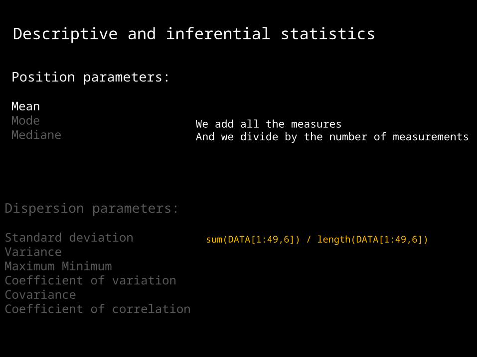
Position parameters:

MeanModeMediane

Dispersion parameters:

Standard deviationVarianceMaximum MinimumCoefficient of variationCovarianceCoefficient of correlation

We add all the measuresAnd we divide by the number of measurements

𝑋= ∑𝑖=1

𝑛

𝑥𝑖



MeanModeMediane



𝑋= 1𝑁 ∑

𝑖=1

𝑛

𝑥𝑖




MeanModeMediane



𝑋= 1𝑁 ∑

𝑖=1

𝑛

𝑥𝑖


sum(DATA[1:49,6]) / length(DATA[1:49,6])



MeanModeMediane



𝑋= 1𝑁 ∑

𝑖=1

𝑛

𝑥𝑖



mean(DATA[1:49,6])



MeanModeMediane



𝑋= 1𝑁 ∑

𝑖=1

𝑛

𝑥𝑖



mean(DATA[1:49,6])

colMeans(DATA[1:49,6:11])


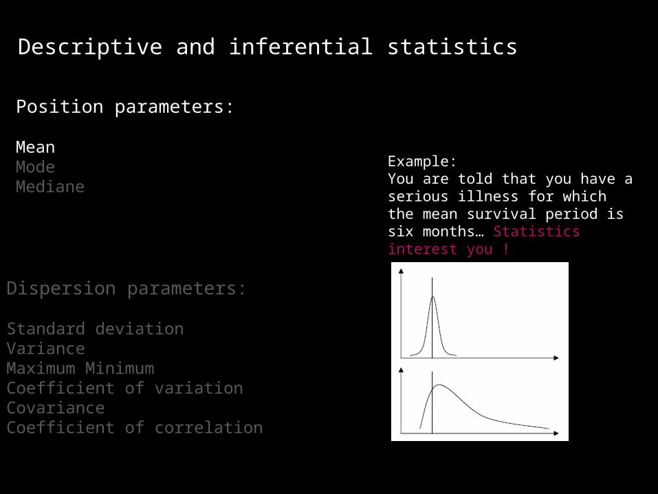
Example:You are told that you have a serious illness for which the mean survival period is six months… Statistics interest you !


MeanModeMediane





MeanModeMediane



The Mode is the most frequent value

Sample > Median = Median < sample



MeanModeMediane





median(DATA[1:49,6])



MeanModeMediane





median(DATA[1:49,6]) quantile(DATA[1:49,6])



MeanModeMediane






min(DATA[1:49,6])max(DATA[1:49,6])



MeanModeMediane






min(DATA[1:49,6])max(DATA[1:49,6])range(DATA[1:49,6])



MeanModeMediane







MeanModeMediane



We calculate the difference between every value and the meanWe square this differenceWe sum the squared differencesAnd we divide by the number of value

𝜎 ²= 1𝑛−1

.∑𝑖=1

𝑛

(𝑥𝑖−𝑋 ) ²



MeanModeMediane




𝜎 ²= 1𝑁−1

.∑𝑖=1

𝑛

(𝑥𝑖−𝑋 )²



MeanModeMediane




𝜎 ²= 1𝑁−1

.∑𝑖=1

𝑛

(𝑥𝑖−𝑋 )²

The variance is the mean of the squared differences to the mean



MeanModeMediane



𝜎=√ 1𝑁−1

.∑𝑖=1

𝑛

(𝑥𝑖−𝑋 ) ²

The standard deviation is the square root of the variance



MeanModeMediane





MeanModeMediane



𝑐𝑣=𝜎𝑋

Transform the standard deviation into the metrics of the variable

It permits to compare two variablesProblem: when X is close to zero, it becomes useless



MeanModeMediane



𝑧=(𝑥−𝑋 )

𝑠

To measure the difference to the mean in the standard deviationmetrics, we use:

This is the centered- reduced variable of mean=0 and variance=1



MeanModeMediane





MeanModeMediane



Covariance measures the degree of dependance of two variables: Are the values of each measurement drift independantly away from the centre of gravity, or are they drifting away together?If x and y are independant, then the covariance is equal to 0



MeanModeMediane




𝑆𝑥𝑦=∑𝑖=1

𝑛

(𝑥𝑖−𝑋 𝑥)(𝑦 𝑖−𝑋 𝑦)

𝑛

We multiply the x-deviation to the mean to its associated y-deviationWe sum these productsWe divide by the number of values



MeanModeMediane





𝑛


𝑛

We multiply the x-deviation to the mean to its associated y-deviationWe sum these productsWe divide by the number of values

So covariance is the sum of the crossed products



MeanModeMediane




𝑛


𝑛


( sum(DATA[1:49,6] * DATA[1:49,7]) - prod(sum(DATA[1:49,6]),sum(DATA[1:49,7])) / length(DATA[1:49,6]) ) / ( length(DATA[1:49,6])-1 )



MeanModeMediane




𝑛


𝑛


( sum(DATA[1:49,6] * DATA[1:49,7]) - prod(sum(DATA[1:49,6]),sum(DATA[1:49,7])) / length(DATA[1:49,6]) ) / ( length(DATA[1:49,6])-1 )

Cov(DATA[1:49,6],DATA[1:49,7])



MeanModeMediane



Pearson’s correlation coefficient differs from the covariance by its absence of unit and its boundaries between -1 and 1

𝑟 𝑥𝑦=𝑆𝑥𝑦

𝑆𝑥×𝑆𝑦



MeanModeMediane





𝑆𝑥×𝑆𝑦

cov(DATA[1:49,6],DATA[1:49,7]) / (sd(DATA[1:49,6]) * sd(DATA[1:49,7]))



MeanModeMediane





𝑆𝑥×𝑆𝑦

cov(DATA[1:49,6],DATA[1:49,7]) / (sd(DATA[1:49,6]) * sd(DATA[1:49,7]))

Cor(DATA[1:49,6],DATA[1:49,7])

introduction to r, statistics, and the grammar of graphics thomas ingicco e. delacroix, dante et...

Documents

data vector series of

dante et virgile aux

hell classes