introduction to recurrence plots in...

Introduction to Recurrence Plots in Matlab

Professor Janet Wiles School of Information Technology and Electrical Engineering

University of Queensland

Tutorial presented at the TDLC Fellows Institute 9th August 2012 Matlab code and graphics by Ting Ting (Amy) Gibson

p 2. Recurrence plots in Matlab, Tutorial presented at the TDLC Fellows Institute 9th August 2012

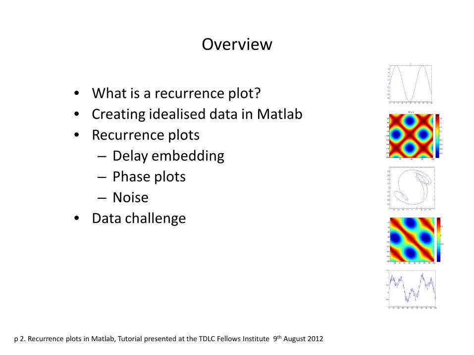
Overview

• What is a recurrence plot? • Creating idealised data in Matlab • Recurrence plots

– Delay embedding – Phase plots – Noise

• Data challenge


What is a recurrence plot?

Given a time series x(t), t = 1, 2,…

a recurrence plot shows when the time series visits the same region of phase space:

x(i) ~= x(j) where i indexes time

on the x-axis and j indexes time on the y-axis.

time

time


Recurrence plot showing neurons in conversation in parietal cortex

Graphics: Amy Gibson Data: Doug Nitz

Recurrence plot of the day Recurrence plots of ECG data of cardiac patients after heart surgery

www.recurrence-plot.tk/rp_of_the_day.php

Embedding and recurrence plot parameters: (left) m=3 , τ=20 , ε=0.030 (created: 2012-05-30); (right) m=2 , τ=14 , ε=0.030 (created: 2012-05-24) Data from the German Heart Centre Munich.


Task 1a. Create a time series: An ideal LFP can be represented as a sine wave, e.g. theta (8Hz) frequency for 200 msec a = sin((1:200)*2*pi*8/1000); plot(a);

Task 1b: Try different frequencies e.g. for 23Hz beta frequency use 23/1000 Task 1c: Add 2 frequencies and plot b = 0.6*a + 0.4*sin((1:200)*2*pi*23/1000); Notes • The power of a frequency, f, is typically proportional to 1/f • How would you create an LFP signal with 200ms of theta

(8Hz) followed by 200 ms of beta (23Hz)?

Time series data


Task 2a. Create a distance plot: imagesc(1-dist(a)); colorbar; axis square;

Task 2b. Create a recurrence plot with threshold 0.9: imagesc((1-dist(a))>0.9); colormap([1 1 1; 0 0 0]);

Task 2c: Vary the threshold

Task 2d: Calculate the average recurrence: sum(sum((1-dist(a))>0.9))/(200*200)

Notes • Recurrence plots (RPs) are traditionally black and white • How does the average recurrence change with the threshold?

Recurrence Plots (RP)


Refining the recurrence plot: To match the trajectory (the direction the signal is moving)

we create a time delayed copy of the signal

x(i, i+τ) ~= x(j, j+τ)

Definitions: The time delay is τ (pronounced tau), default τ=1. The embedding dimension, m, is the number of time delayed copies of the signal used to track the trajectory, default m=1.


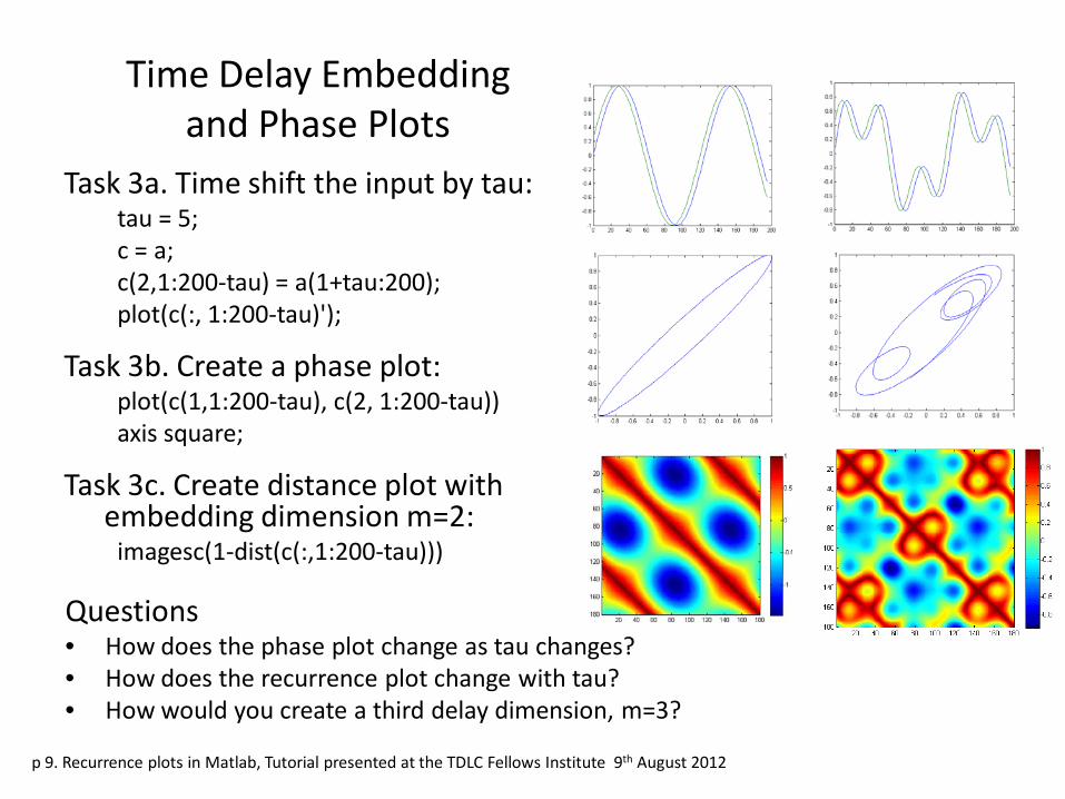
Task 3a. Time shift the input by tau: tau = 5; c = a; c(2,1:200-tau) = a(1+tau:200); plot(c(:, 1:200-tau)');

Task 3b. Create a phase plot: plot(c(1,1:200-tau), c(2, 1:200-tau)) axis square;

Task 3c. Create distance plot with embedding dimension m=2:

imagesc(1-dist(c(:,1:200-tau)))

Time Delay Embedding and Phase Plots

Questions • How does the phase plot change as tau changes? • How does the recurrence plot change with tau? • How would you create a third delay dimension, m=3?


Task 4a. Autocorrelation plot(xcorr(a));

Task 4b. Set tau equal to the distance (on the x-

axis) between the center peak and the first local minima. Replot the phase plot from Task 3

Questions • What is the relationship between tau and sine

wave frequencies? • What does the autocorrelation of nested sine

waves look like? • Explore the phase plots for different time shifts

(tau) based on interesting values found on xcorr

Use autocorrelation to find the optimal time delay for the phase plot

τ


Task 5a. Add noise to the data

Uniform random noise: c = a + rand(1,200);

High frequency noise (100Hz): d = a + 0.2*sin((1:200)*2*pi*100/1000);

Task 5b.Plot the time series and the recurrence plots.

Task 5c. Add noise to the nested frequency data.

Noise in Recurrence Plots

Random noise 100Hz noise


Noise in Recurrence Plots

(cont)

Task 5c. Add noise to the nested frequency data; recalculate the autocorrelation and recurrence plot

Questions • What effect does noise

have on auto-correlation? • What effect does noise

have on RPs using time delay embedding m=2?

Random noise 100Hz noise


Local Field Potential (LFP) challenge

• Create a “realistic” LFP for a rat repeatedly running to an object, being rewarded with a food pellet and running back; composed of a series of theta, beta and gamma frequencies with variable length sequences of chew artefact and other uniform random noise:

f8 = 1/8 * sin((1:500) * 2 * pi * 8/1000); when the rat is running f17 = 1/17 * sin((1:120) * 2 * pi * 17/1000); occasionally f23 = 1/23 * sin((1:120) * 2 * pi * 23/1000); when the rat is rewarded f41 = 1/41 * sin((1:200) * 2 * pi * 41/1000); when the rat is perceiving chew = 1/10 * rand(1,125); after reaching the object fnested = 1/8*sin((1:200)*2*pi*8/1000) +

1/41*sin((1:200)*2*pi*41/1000) + 1/60*rand(1,200); combinations of the above

• How would you create a recurrence plot that showed the transitions

between different LFP states?


Advanced topics

• Other types of recurrence http://www.nsf.gov/sbe/bcs/pac/nmbs/chap2.pdf (good overview)

– Cross recurrence plot – Joint recurrence plot – Conceptual recurrence plots (Discursis)

Angus, Smith & Wiles (2012a). http://dx.doi.org/10.1109/TVCG.2011.100 • Quantification

– Recurrence quantification analysis (RQA) Webber & Zbilut (1994). www.nsf.gov/sbe/bcs/pac/nmbs/chap2.pdf

– Multi-participant recurrence (MPR) metrics Angus, Smith & Wiles (2012b). http://dx.doi.org/10.1109/TASL.2012.2189566

• Theory – Eckmann, Kamphorst & Ruelle (1987).

http://dx.doi.org/10.1209/0295-5075/4/9/004 (original reference) – Kulkarni, Marwan, Parrott, Proulx, Webber (2011).

http://dx.doi.org/10.1142/S0218127411029057 (complex systems overview) – Takens’ theorem and embedding dimensions

• Websites – Discursis website www.discursis.com – Recurrence plot website www.recurrence-plot.tk

http://www.nsf.gov/sbe/bcs/pac/nmbs/chap2.pdf�

http://dx.doi.org/10.1109/TVCG.2011.100�

http://www.nsf.gov/sbe/bcs/pac/nmbs/chap2.pdf�

http://dx.doi.org/10.1109/TASL.2012.2189566�

http://dx.doi.org/10.1209/0295-5075/4/9/004�

http://dx.doi.org/10.1142/S0218127411029057�

http://www.discursis.com/�

http://www.recurrence-plot.tk/�


Acknowledgements

Thanks to Ting Ting (Amy) Gibson for the Matlab code and figures

Funding for this tutorial was provided by

Australian Research Council NSF Temporal Dynamics of Learning Center

Kavli Institute for Brain and Mind

introduction to recurrence plots in...

Documents