SCILAB- An Introduction

Dr. Balasaheb M. Patre,Professor and Head,

Balasaheb M. Patre 2010 © SGGSIE&T, Nanded 1

Professor and Head,Department of Instrumentation Engineering,SGGS Institute of Engineering and Technology,Vishnupuri, Nanded-431606.E-mail: bmpatre@yahoo.com

What is SCILAB?

(1) SCILAB is a freely distributed and open source scientific software package

(2) A powerful open computing environment for Engineering and Scientific applications

(3) Developed since 1990 by researchers from INRIA

2

(3) Developed since 1990 by researchers from INRIA (Institut Nationale de Recherche en Informatique et en Automatique) and ENPC (National School of Bridges and Roads).

(4) Now maintained and developed by Scilab consortium since 2003.

(5) Integrated into Digiteo foundation in July 2008(6) The current version is 5.2.1 (February 2010)

What is SCILAB? …contd

7) Since 1994 it is distributed freely along with source code through the Internet. (www.scilab.org)

8) Scilab users can develop their own module so that they can solve their particular problems.

3

they can solve their particular problems.

7) The Scilab language allows to dynamically compile and link other languages such as Fortran and C: this way, external libraries can be used as if they were a part of Scilab built-in features.

8) Scilab also interfaces LabVIEW, a platform and development environment for a visual programming language from National Instruments.

Scilab’s Main Features:

1. A high-level programming language2. Scilab is an interpreted language3. Integarated object-oriented 2-D and 3-D graphics

with animationA dedicated Editor

4

4. A dedicated Editor5. An XML-based help system6. Interface with symbolic computing packages (Maple

and MuPAD 3.0)7. An interface with Tcl/Tk8. Scilab works with most Unix systems including

GNU/Linux and on Windows (9X/NT/2000/XP/Vista/7), and Mac operating system

Scilab coded Toolboxes1. Linear algebra and Sparse matrices2. Polynomials and Rational functions3. 2-D and 3-D graphics with animation4. Interpolation and Approximations5. Linear, Quadratic and Nonlinear Optimization

ODE solver and DAE solver

5

6. ODE solver and DAE solver7. Classical and Robust Control, LMI Optimization8. Differentiable and Non-differential Optimization9. Signal Processing10. Statistic11. Scicos: A hybrid dynamic system modeler and

simulator12. Parallel Scialab using PVM13. Metanet: Graphs and Networks

Typical uses� Educational Institutes, Research centers and companies� Math and computation� Algorithm development� Modeling, simulation, and visualization

6

� Modeling, simulation, and visualization� Scientific and engineering graphics, exported to variousformats so that can be included into documents.

� Application development, including GUI building

Basic data element (Matrix)Array : not require dimensioningAllow to solve problem with matrix and vector formulations

Desktop tool and development environmentSet of tools and facilitiesGraphical UI : Scilab Console, Sciab editor, Scilab help bowser, MATLAB to Scilab TranslatorMathematics Function LibraryCollection of computational algorithm : sum, sine, matrix

7

Collection of computational algorithm : sum, sine, matrix functionsLanguageHigh-level matrix/array language with flow, functions, structureGraphicsExtensive facilities for displaying vectors and matrices as graphsHigh-level functions for 2-D and 3-D data visualizationExternal InterfacesAllows to write C and Fortran programs that interact with SCILAB

Getting Started with Scilab

Stating the Scilab program

� Start the Scilab program by double-clicking Scilab-5.2.1 icon on thedesktop

� Start button on the desktop >Programs>Scilab-5.2.1>Scilab-5.2.1

8

� Start button on the desktop >Programs>Scilab-5.2.1>Scilab-5.2.1Automatically loadingTools for managing files, variables and applications

Quitting the Scilab program

� To end SCILAB, File > quit in the scilab console� Type ‘quit’ in the Scilab Console� The user enters commands at the prompt ---->

Scilab Default Console

9

Scilab Help Browser

10

Help FeaturesTo open SCILAB help, click help icon (?) in the toolbar or type help at

the command prompt ----->

� Help Browser

� help command (help inv, help optim)

11

(This is useful when the name of the function is already Known)

� To obtain a list of Scilab functions corresponding to a keyword,

the command apropos followed by the keyword should be used.

-->apropos eigenvalues <Enter>� Help can also be from Scilab demonstrations

� This is available from the console, in the menu ? > Scilab Demonstrations.

Scilab Demos Window

12

Arithmetic Operations:� + addition

� - subtraction

� * multiplication

/ right division i.e.

13

� / right division i.e.

� \ left division i.e.

� ^ power i.e.

� ** power (same as ^)

� ' transpose conjugate

1/X Y XY

−

=

1\X Y X Y

−

=

YX

Scilab as a Calculator-->6+5ans =

11.

-->6+5;

-->4+5/3+2ans =

7.6666667

-->5^3/2ans =

14

-->7+8/2ans =

11.

-->(7+8)/2ans =

7.5

62.5

-->27^(1/3)+32^0.2ans =

5.

-->27^1/3+32^0.2ans =

11.

Scilab as a Calculator

-->0.7854-(0.7854)^3/(1*2*3)+0.785^5/(1*2*3*4*5)..-->-(0.785)^7/(1*2*3*4*5*6*7)ans =

0.7071016

-->// This is my comment .

15

-->// This is my comment .

� In Scilab, any line which ends with two dots is considered to be the start of a new continuation line.

� Any line which begins with two slashes "//" is considered by Scilab as a comment and is ignored.

� More than one command can be entered on the same line by separating the commands by semicolon (;) or a comma (,)

Background - computersOutput

16Input

Background - hardware

MemoryCPU

17

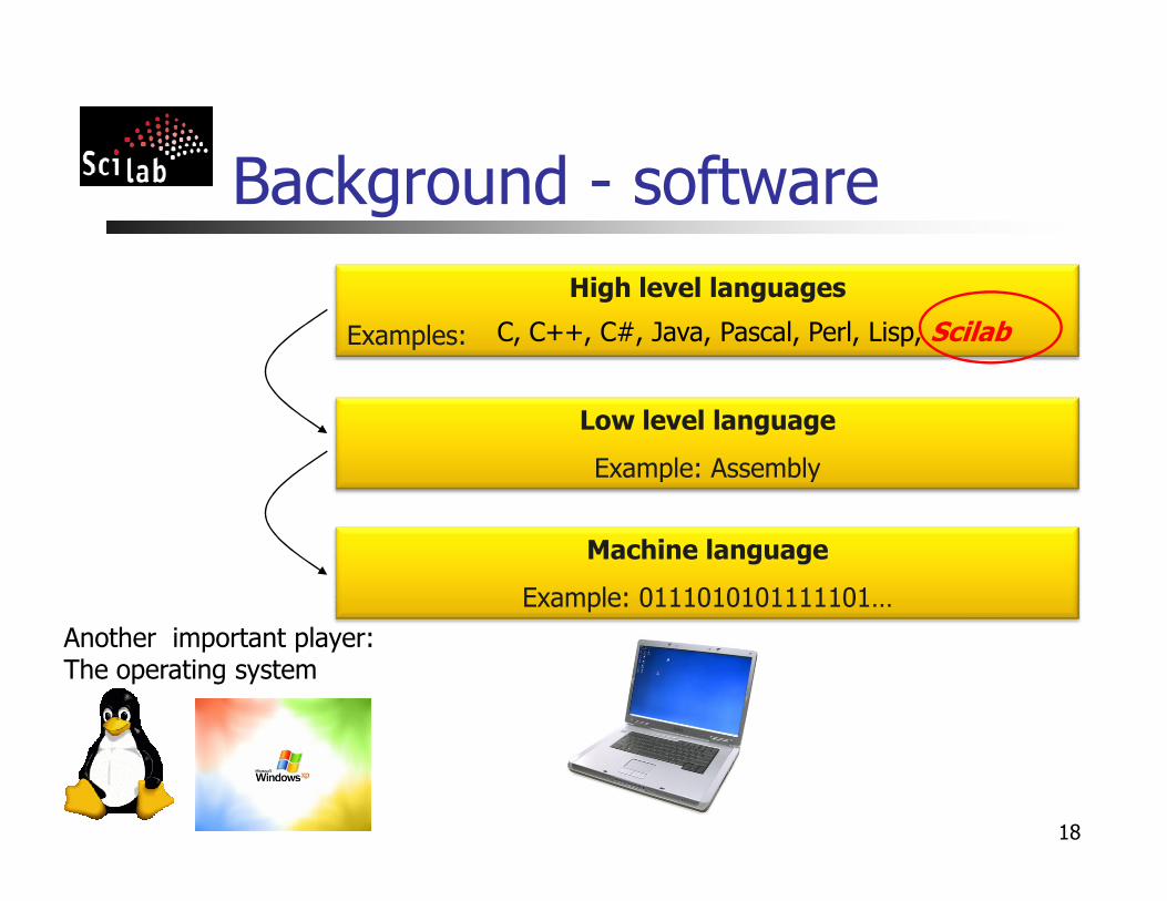
Background - software

Low level language

Example: Assembly

High level languages

Examples: C, C++, C#, Java, Pascal, Perl, Lisp, Scilab

18

Machine language

Example: 0111010101111101…

Example: Assembly

Another important player: The operating system

Basic Elements of Scilab:� In Scilab, everything is a matrix

� All real, complex, Boolean, integer, string, and polynomial variables are matrices.

� Scilab is an interpreted language, which implies that there is no need to declare a variable before using it. Variables are created at the moment where they are first set.

In Scilab “=“ sign is called assignment operator.� In Scilab “=“ sign is called assignment operator.

-->x=10 10 is assigned to variable x

x =

10.

-->x=3*x-12 A new value is assigned to x. The new values is

x = three time of previous value of x minus 12.

18.

� Varaiable names may be as long as user wants but only first 24 characters are taken into account.

� Scilab is case sensitive. A is not equal to a.

19

Predefined Variables:

Certain variables are predefined and write-protected� %i i = √−1 immaginary unit

� %pi = 3.1415927 . . . pi grek

� %e e = 2.718281 . . . number of Nepero

� %eps = precision (machine dependent)

π

ε 1 62 .2 1 0

−

×

20

� %eps = precision (machine dependent)

� %inf infinity

� %nan NotANumber

� %s s polynomial variable

� %z z polynomial variable

� %t true boolean variable

� %f false boolean variable

ε 1 62 .2 1 0

−

×

Some useful Scilab Commands

General commands:� clock Provide clock time and date as a vector [year month day

hour minute seconds] -->clock

ans =

2010. 4. 20. 23. 38. 59.2010. 4. 20. 23. 38. 59.

� date Current date a string-->dateans =20-Apr-2010

� ver Version information for Scilab -->verans =!Scilab Version: 5.2.0.1266391513 !

21

Some useful Scilab Commands ……contd.

� Workspace Commands:who Lists the variables currently in the scilab workspacewhos Same a who but provides more information on size, typewhos -type constants List the variables that can store real or

complex constantcomplex constantWhos –name a List all variables with name starting with the letter ‘a’what Lists the scilab primitivesclear Kills the variables which are not protected. clear xyz Kills the variables specified in the commandclc Clears screenclf Clears figure windowdiary List of current session commands

22

Some useful Scilab commands ….contd

� Directory commands:pwd Provides scilab current working directory-->pwdans =C:\Program Files\scilab-5.2.1C:\Program Files\scilab-5.2.1

copyfile Copies a file

mkdir Makes a a new directory/folder in the current directory

� Termination Commands:quit Quits Scilabexit Same as quit command

23

Creating Arrays (Vectors and Matrices)-->a=[1 2 3 4 5 6 7 8 9 10] Create a row vector

a =

1. 2. 3. 4. 5. 6. 7. 8. 9. 10.

-->a=[1,2,3,4,5,6,7,8,9,10] Another way of creating a row vector

a =

1. 2. 3. 4. 5. 6. 7. 8. 9. 10. 1. 2. 3. 4. 5. 6. 7. 8. 9. 10.

-->a=[1;2;3;4;5;6;7;8;9;10] Create a column vectora =

1.

2.

3.

4.

5.

6.

7.

8.

9.

10.

24

Vectors and matrices ……contd.

Variable_name=m:q:n (m=first term, q=spacing, n=last term)-->a=1:10 Creating a row vector with colon (:) operatora = Default incerment is one

1. 2. 3. 4. 5. 6. 7. 8. 9. 10. -->a=1:1:10 Specified increment is onea =a =

1. 2. 3. 4. 5. 6. 7. 8. 9. 10. -->a=1:2:11 Specified increment is twoa =

1. 3. 5. 7. 9. 11. -->a=100:-10:0 Specified increment is -10.a =

100. 90. 80. 70. 60. 50. 40. 30. 20. 10. 0.

25

Vectors and matrices ……contd.-->a=[2+3*%i, 4+1*%i, 3, 5, 6] Vector with complex numbersa =

2. + 3.i 4. + i 3. 5. 6. -->b=[1+6*%i, 4+6*%i 3, 4, 6]b =

1. + 6.i 4. + 6.i 3. 4. 6. -->c=a+b Vector addition-->c=a+b Vector additionc =

3. + 9.i 8. + 7.i 6. 9. 12. -->a-b Vector subtractionans =

1. - 3.i - 5.i 0 1. 0 -->a*b!--error 10

Inconsistent multiplication.

26

Vectors and matrices ……contd.-->a=linspace(0,10,5) Generates a vector of 5 elements, 0 is the first

element and 10 is the last elementa =

0. 2.5 5. 7.5 10. -->a=logspace(0,4,3) Generates a logarithmically spaced vector of length

3 between a =

0 41 0 to 1 0

a =1. 100. 10000.

-->a=[1 10 25 50 15]a =1. 10. 25. 50. 15.

-->a(3) Addressing a vector elementans =

25.

27

1 0 to 1 0

Vectors and matrices ……contd.-->a=[1 10 25 50 15]a =

1. 10. 25. 50. 15.

-->b=sum(a) Sum of all elementsb =101. 101.

-->c=mean(a) Average of the elementsc =

20.2 -->d=length(a) Number of elements in the vectord =

5. -->e=max(a) Maximum value in the vectore =

50. 28

Vectors and matrices ……contd.-->f=min(a) Minimum value in the vectorf =

1. -->g=prod(a) Product of elements in the vectorg =

187500. -->h=sign(a) Returns 1 if the sign of an element is the-->h=sign(a) Returns 1 if the sign of an element is the

vector is +ve, 0 if element is 0, -1 if the element is –ve.h =

1. 1. 1. 1. 1. -->i=find(a) Returns the indices corresponding to the non-zero

entry of the array ai =

1. 2. 3. 4. 5.

29

Vectors and matrices ……contd.-->p=[1.4 10.7 -1.1 20.9]p =

1.4 10.7 - 1.1 20.9 -->a=fix(p) Rounds the elements of the vector p to the nearest

integer towards zeroa =

1. 10. - 1. 20.-->b=floor(p) Rounds the elements of the vector p to the nearest-->b=floor(p) Rounds the elements of the vector p to the nearest

integer towards b =

1. 10. - 2. 20. -->c=ceil(p) Rounds the elements of the vector p to the nearest

integer towards c =

2. 11. - 1. 21. -->d=round(p) Rounds the elements of the vector p to the nearest integer d =

1. 11. - 1. 21.-->e=gsort(p) Sorts the eleemnts of p in descending ordere =

20.9 10.7 1.4 - 1.1

30

−∞

+∞

Vectors and matrices ……contd.

-->A=[16 3 2 13;5 10 11 8;9 6 7 12;4 15 14 1] Entering a matrixA = use space or , for row elements

16. 3. 2. 13. use ; to terminate a row5. 10. 11. 8. 9. 6. 7. 12. 4. 15. 14. 1.

-->B=sum(A) Gives the sum of all the elements-->B=sum(A) Gives the sum of all the elementsB =

136. -->C=sum(A,'c') Sum of the elements of columnC =34. 34. 34. 34.

-->D=sum(A,'r') Sum of the row elementsD =

34. 34. 34. 34.

31

Matrix Addressing:

-->A=[3 11 6 5;4 7 10 2;13 9 0 8]A =3. 11. 6. 5. 4. 7. 10. 2. 13. 9. 0. 8. 13. 9. 0. 8.

-->A(2,3)ans =

10. -->A(:,2)ans =

11. 7. 9.

32

Matrix Addressing-->A(2,:)ans =

4. 7. 10. 2.

-->A(9)-->A(9)ans =

0.

-->A(1:2,1:2)ans =

3. 11. 4. 7.

33

Vectors and matrices ……contd.-->B=A(3:-1:1,1:4)B =13. 9. 0. 8. 4. 7. 10. 2. 3. 11. 6. 5.

-->B=A(3:-1:1,1:4)-->B=A(3:-1:1,1:4)B =13. 9. 0. 8. 4. 7. 10. 2. 3. 11. 6. 5.

-->A(1:3,4)=[]A =

3. 11. 6. 4. 7. 10. 13. 9. 0.

34

Vectors and matrices ……contd.-->eye(2,2)ans =1. 0. 0. 1.

-->ones(2,3)ans =1. 1. 1. 1. 1. 1. 1. 1. 1.

-->zeros(3,3)ans =0. 0. 0. 0. 0. 0. 0. 0. 0.

-->A=[1 2;3 4]; B=[2 3; 5 6];-->C=[A,B]C =

1. 2. 2. 3.

3. 4. 5. 6.

35

Vectors and matrices ……contd.-->A=rand(2,3)A =

0.8497452 0.8782165 0.5608486 0.6857310 0.0683740 0.6623569

-->A=[1 2 3; 4 5 6;7 8 9];-->B=diag(A)B =B =1. 5. 9.

-->C=diag(A,1)C =

2. 6.

-->D=diag(A,-1)D =

4. 8.

36

Vectors and matrices ……contd.-->A=[1 2;0 4]; -->det(A)

ans =4.

-->rank(A)ans =2. -->trace(A)

ans =ans =5.

-->B=inv(A)B =

1. - 0.5 0. 0.25

-->norm(A)ans =

4.495358 -->C=A'C =1. 0. 2. 4.

37

Vectors and matrices ……contd.-->p=poly(A,'x')p =

2 4 - 5x + x

-->q=spec(A)q =

1. 1. 4.

ans =0. 0. 0. 0. 0. 0. 0. 0. 0.

-->A=[1 2;3 4]; B=[2 3; 5 6];-->C=[A,B]C =

1. 2. 2. 3.

3. 4. 5. 6.

38

Vectors and matrices ……contd.

Matrix operators and elementwise operators

� + addition .+ elementwise addition

� - substraction .- elementwise substraction

� * multiplication .* elementwise multiplication

� / right division ./ elementwise right division

� \ left division .\ elementwise left division

� ^ or ** power .^ elementwise power

� ' transpose and conjugate .' transpose (but not

conjugate)

39

Scilab Editor � When several commands are to be executed, it may be more

convenient to write these statements into a file with Scilab editor. To execute the commands located in such a file, the exec function can be used, followed by the name of the script. This file generally has the extension .sce or .sci, depending on its content:

� Files having the .sci extension are containing Scilab functions and

40

� Files having the .sci extension are containing Scilab functions and executing them loads the functions into Scilab environment (but does not execute them),

� Files having the .sce extension are containing both Scilab functions and executable statements.

� Executing a .sce file has generally an effect such as computing several variables and displaying the results in the console, creating 2D plots, reading or writing into a file, etc...

Our first script (Sce-file)The editor can be accessed from the menu of the console, under the Applications > Editor menu, or from the console as:--> editor ()

41

Another Script File

42

Scilab Functions � It is possible to define new functions in the scilab.

� To dene a new function, we use the function and endfunction Scilab keywords.

function y = myfunction ( x )

y = 2 * x

endfunction

43

endfunction

-->y=myfunction(3)

y =

6.

-->y=myfunction(8)

y =

16.

Scilab Functions …contd. � Functions can have an arbitrary number of input and

output arguments so that the complete syntax for a function which has a fixed number of arguments is the following:

[o1 , ... , on] = myfunction ( i1 , ... , in )

44

[o1 , ... , on] = myfunction ( i1 , ... , in )

� The input and output arguments are separated by commas ",". Notice that the input arguments are surrounded by opening and closing braces, while the output arguments are surrounded by opening and closing square braces .

Computer precision limitations

� How much is:

-->0.42 + 0.08 - 0.5

ans =

0.

� -->0.42 - 0.5 + 0.08

ans =

- 1.388D-17

45

Polynomials� A polynomial can be created in two ways. One way is to define

the polynomial in terms of its roots and the other way is to define it in terms of its coefficients.

-->p1 = poly([-1 -2], 'x')

p1 =

2

46

2

2 + 3x + x

-->p1 = poly([-1 -2], 'x', 'r')

p1 =

2

2 + 3x + x

-->p2 = poly([2 3 1], 'x', 'c')

p2 =

2

2 + 3x + x

Polynomials …contd.-->roots(p1)

ans =

- 1.

- 2.

-->p3=p1+p2

p3 =

47

p3 =

2

4 + 6x + 2x

-->p4=p1*p2

p4 =

2 3 4

4 + 12x + 13x + 6x + x

-->p1==p2

ans =

T

Polynomials ….contd-->coeff(p1)

ans =

2. 3. 1.

-->derivat(p1)

ans =

3 + 2x

48

3 + 2x

-->c=companion(p1)

c =

- 3. - 2.

1. 0.

-->spec(c)

ans =

- 2.

- 1.

Polynomials …contd.->p6=poly(c,'x')

p6 =

2

2 + 3x + x

-->p=(1+2*x+3*x^2)/(4+5*x+6*x^2)

p =

49

p =

2

1 + 2x + 3x

----------- ------

2

4 + 5x + 6x

-->numer(p)

ans =

2

1 + 2x + 3x

Plotting Graphs (1)

-->x=[0:%pi/16:2*%pi]';

-->y=[cos(x) sin(x)];

50

-->plot2d(x,y)

-->xgrid

-->xlabel('x')

-->ylabel('sin(x), cos(x)')

Plotting Graphs (2)

51

Plotting Graphs (3)

-->x=[0:%pi/32:2*%pi]';

-->y=[cos(x) sin(x) cos(x)+sin(x)];

52

-->plot(x, y); xgrid(1);

-->xtitle('TRIGINOMETRIC FUNCTIONS', 'x', 'f(x)');

-->legend('cos(x)', 'sin(x)', 'cos(x) + sin(x)', 1, %F);

Plotting Graphs (4)

53

Conclusions

� Scilab is a non-commercial open source platform for Engineering and Scientific computations.

� Scilab is ideal for educational institutes, schools and industries.

54

� Scilab/Scicos is a better alternative for Matlab/Simulink.

� Students can perform mathematical computations, algorithm development, simulation, prototyping, and data analysis using scilab.

� A valuable tool for researchers at no cost.

THANK YOUTHANK YOU

55