Kolkata, December, 2018

Introduction to sensitivityanalysis

Bertrand Iooss(EDF R&D & Institut de Mathématiques de Toulouse, France)

Environnemental variables Physical parameters Parameters of process

Distributions of outputs Probability of failure Most influent inputsCalibrating the input parameters

Computer codeor

Experiment

Using « Best-estimate » computer codes in engineering

Exploratory studies: understand a phenomenon, an experim/indust. process

Safety studies: compute a failure risk (margins, rare events) and prioritize the riskindicators, with validated computer models

Design studies: optimize and manage the system performances

Cost ($€, cpu, …) potentially large

X1

X2

Z Q95%

Uncertainties

Possible needs of metamodel

Design of experiments

Z=G(X1, …, Xp)

Step B:Quantification of uncertainty

sources

Direct methods, statistics, expertise

Model G(x)

(or measurement

process)

Input

variables

Uncertain : x

Variables

of interest

Y = G(x)

Step A : Problem specification Quantity of

interest

Ex: variance, probability,

maximum, arg max, …

Step C : Uncertainty propagationDesign of experiments

Step C’ : Sensitivity analysis, Prioritization

Observed variables

Yobs

Step B’: Quantification of sourcesInverse methods, calibration, assimilation

Metamodel

UQ methodology

Example: Garonne flood risk (TELEMAC code Uncertainty analysis

Global analysis

Convergence and confidence intervals at 95 %

of the estimated mean

Empirical PDF based on 70 000 simulations

local analysis

[ Goeury et al., 2015 ]

SCF4

Global analysis : First order indices of Sobol

local analysis

• The flowrate input factor explains about 80% ofthe variance of the output variable

• Few interactions between the uncertainvariables

[ Goeury et al., 2015 ]

Industrial example: Garonne flood riskSensitivity analysis

Sensitivity analysis notions

Sensitivity, for example

Answer to: how the output varies with respect to potential perturbations of the inputs?

Contribution = sensitivity x importance, for example

Gives the weight of an input (or group of inputs) on the uncertainty of the output

The input contributions are often called “importance measures”, “sensitivity indices”, …

iXZ

)( i

i

XX

Z

DX DZ

G

XZ

The model :

Z = G (X1, …, Xp)

Quadratic combination methodIndependent case

Quadratic summation formula

If the Xi (i = 1…p) are independent, by using the first-order Taylor decompositionof Z around m (linearization), we obtain:

Contribution of each input variable to the uncertainty of the output variable

Sensitivity indices (normalized)

2

1

2

)(Var i

p

iXjX

GZ

m

2

2

2

)(Var

1i

Xi

iX

G

Z

m

Sensitivity analysis is directly obtained

Computation of derivatives via finite differences, exact differentiation, or automatic differentiation

Main objectives of sensitivity analysis (SA)1. Understand the behaviour of the model (decompose input-output relations)

2. Simplify the computer model (dimension reduction)

Determine the non-influent variables (that can be fixed)

Determine the non-influent phenomena (to skip in the analysis)

Build a simplified model, a metamodel

3. Prioritize the uncertainty sources to reduce the model output uncertainty

- Variables to be fixed to obtain the largest output uncert. reduction

- Most influent variables in a given output domain

4. Analyze the robustness of the quantity of interest (QoI) with respect to the input uncertainty laws

Quantitative partitioning

Screening

Robustnessanalysis

(QoI= variability of the output)

Three types of answers:

1. Screening (qualitative information: influent/non influent)

- classical design of experiments,

- numerical design of experiments (Morris, sequential bifurcation)

2. Quantitative measures of global influence

- correlation/regression on values/ranks,

- functional variance decomposition (Sobol)

3. Deep exploration of sensitivities

- smoothing techniques (param./non parametric)

- metamodels

Methodology of SA

X1

X3

X2

Z

[ Kleijnen 2008,

Saltelli et al. 2008,

Storlie et al. 2010, … ]

Outline

1. Design of experiments

2. Global sensitivity analysis

2.1 Screening

2.2 Sampling-based approaches

2.3 More advanced methods

X1

X2

Screening without hypothesis on function: Morris’ method

• Discretization of input space

• Computation of one elementary effect for eachinput

P1

• Needs p + 1 experiments

• OAT (One-at-A-Time)

P2P3

X1

X2

1

5

4

3

2

• OAT design is repeated R times (total: n = R*(p+1) experiments)

• It gives an R-sample for eachelementary effect

• Sensitivity measures:

Morris’ method

Morris: Sensitivity measures

• is a measure of the sensitivity:

Important value important effects (in mean) sensitive model to input variations

• is a measure of the interactionsand of the non linear effects:

important value different effects in the R-sample effects which depend on the value:

• of the input Xi => non linear effect• or of the other inputs => interaction(the distinction between the two cases is impossible)

Morris: Example

*m

Test case: non monotonic funtion of Morris

20 factors210 simulations Graph (m*,)

Distinction between 3 groups:

1. Negligible effects2. Linear effects3. Non linear effects

and/or with interactions

1

3

2

Example : fuel irradiation computation in HTR

Computer code ATLAS (CEA) : simulation of the HTR fuel(fuel particles) behaviour under irradiation

Noyau de matière fissileCarbone pyrolytique poreuxCarbone pyrolytique denseCarbure de Silicium

Contamination sources: failure of particlesReliability studies are needed

The failure of a particle can be caused by the failure of the external thick layers(IPyC, SiC, OPyC)

Output variables are reprsentative of failure phenomena: maximal orthoradial strainsin external layers

Number of particles inside a reactor : 109 to 1010 !

< 1mm

3 uncertainty types for the inputs• 10 parameters of fuel particle manufacturing process (thickness, …)

Specifications truncated Gaussian distributions

• 5 parameters of irradiation (temperature, …)Interval [min,max] uniform distributions

• 28 behaviour laws (functions of temperature, flux, …)Expert judgment multiplicative constants (~ U[0.95,1.05])

Example : Law of

PyC densification

Results of Morris

Large sensitivities to theseinputs (thickness, irradiation temperature)Small interaction effects

Influence of creep and densification laws of PyC

Conclusion: Morris method provides qualitative information about output variations due to potential variations of inputs

Useful in order to identify the potential influent inputs

p = 43 inputs, 20 repetitions, n = 860 runs, unitary cost ~ 1 mn => total=14h

Outline

1. Design of experiments

2. Global sensitivity analysis

2.1 Screening

2.2 Sampling-based approaches

2.3 More advanced methods

The sampling-based approaches

Sample ( Xp, Z (X ) ) of size N > p

Monte Carlo sample, space filling design, …

[…, Saltelli et al. 2000, Helton et al. 2006, … ]

Preliminary step : graphical visualization (for ex: scatterplots, but also cobweb…)

Example of the OpenTURNS graphical interface

First visualization: scatterplots

YX

YX

),cov(

yx

N

i

ii

ss

yyxxN

1

))((1

0.00 0.02 0.04 0.06 0.08 0.10

02

46

810

i3

p23

N runs

Graphs: Output with respect to each input

Example:N = 300

Measure the linear character of the cloud

Example: Flood model - Scatterplots – Output S

Monte Carlo sample – N = 100

Q = river flowrate ~ Gumbel on [500,3000]

Ks = friction coefficient ~ normal on [15,50]

Zv = downstream river bed heigth ~ triangular on [49,51]

Hd = dyke heigth ~ triangular on [7,9]

Cb = bank heigth ~ triangular on [55,56]

Example: Flood model - Scatterplots – Output Cp

Monte Carlo sample – N = 100

Major drawback: only first order relations between inputs are analyzed and not their interactions (=> needs of other data anlysis tools)

Second visualization: the cobweb plot

Interactive use with the OpenTURNS graphical interface

Sensitivity indices in case of linear inputs/output relation

Independent inputs

Sample: n realizations of

Linear regression model:

Standard Regression Coefficients (SRC) :

Sign of bi gives the direction of variation of Z / Xi

Similar to the linear correlation coefficient (Pearson)

Validity of the linear model

via regression diagnostics and R²:

Theoretically, we have , useful to interpret SRC

p

i

ii XZ1

0 bb

)Var(

)Var(:SRC

Z

XX i

ii b

Y,X

n

i

i

n

i

ii

YY

YY

R

1

2

1

2

2

ˆ1

pX,X ...,1X

p

i

iXR1

22 SRC

A classical view on the « Sampling-based approaches »

Sample ( Xp, Z (X ) ) of size N > p

? Linear relation ?

Yes

Linear regression between X

and Z

Regression coefficients

(R²)

Sensitivityindices

No ? Monotonic relation ?

Yes

Regression on ranks

(R²*)

[…, Saltelli et al. 2000, Helton et al. 2006, … ]

SRRCPRCC

…

SRC are valid sensitivity indices; global sensitivity analysis is achieved

Cp output : R² = 0,83 ; => linear model is not sufficiently valid

Application on the flood model – Output S

R² = 0.98=> Linear model

is valid

36% 16% 29% 0%

12% 0% 3% 0%

Monte Carlo sample – N = 500

Industrial example: Nuclear PWR severe accident study

Important issue for the safety core of the industrial operator

Main questions after a severe accident (PSA level 2):

Is there some radionuclide release outside the containment (and what is the time of this release) ?What is the efficiency of mitigation actions?Influence of the large parameter uncertainties on the failure probability?

Development of a soft simulating severe accident scenarios (corium behavior)

Probabilistic Safety Assessment

Complex and coupled numerical models which require sensitivity analysis to:Identify the main sources of uncertaintiesUnderstand the relations between uncertain inputs and interest outputs

Main objectives of these uncertainty studies

Scenario :

Core degradation, corium transfer and interaction (inside

in-vessel and ex-vessel)

23 Interest output variables :

Corium masses

Time of vessel failure

Time of reactor pit failure

32 input random variables

(uniform laws) :

Water management, physical properties, …

Corium fallsinto the bottom head

Corium concrete interaction

Core degradation and melting

Corium falls into the reactor pit

Additional problem: provide tools for engineers knowing nothing little about stats

3 use levels of the soft – 1) Precise and punctual needsExample: relative study about the failure probability

Goal: understand the influence of water injection in the vessel and/or in the reactor pit during the accident

Random var. X : 22 uniform - 1 binary (for the water presence/absence)N =500 random simulations (LHS design)

Failure probability is estimated by Monte-Carlo methodP(failure without water injection)/ P(failure with water injection) = 2.5This kind of result could help the definition of management strategies

Corium mass Water arrival time

FailureNo failure FailureNo failure

Sensitivity analysisvia boxplots

3 use levels – 2) Detailed analyses for confirmed users

Example: sensitivity analysis related to an output variable (corium mass) with 22 inputs

Goal: understand which input variables strongly affect the corium mass

Rubble fraction in the water

Water flow in the pit

Z

XSRC i

iiVar

Var)sgn(

2

isgn bb

3 use levels – 3) Help to physical model developers

Example: detection of anomalies

Limit factor of the critical flux

Corium mass in thevessel bottom

500 MC simulations

It has allowed to detect that important phenomena related to the corium transfer were not included in the physical model

3 use levels – 3) Help to physical model developers

Example: detection of anomalies

Limit factor of the critical flux

Corium mass in thevessel bottom

500 MC simulations

It has allowed to detect that important phenomena related to the corium transfer were not included in the physical model

Deep analysis using cobweb plots( Thanks to F. Gaudier and URANIE software )

Outline

1. Design of experiments

2. Global sensitivity analysis

2.1 Screening

2.2 Sampling-based approaches

2.3 More advanced methods

Issues in sensitivity analysis

Numerical model’ issues

P1) G (.) is complex: interactions, non linear, discontinuous, …=> Sobol indices, moment-independent measures

P2) G (.) is costly (several minutes - days to compute one evaluation)

=> Metamodel

Model inputs’ issues

P3) p is large : p > 10 … 100 … => Quantitative screening (HSIC, DGSM)

P4) Dependence between inputs => Shapley indices

P5) Uncertainty on inputs’ pdfs (epistemic) => Robustness analysis (PLI)

Model outputs’ issues

P6) Z is not a single scalar, but a high-dimensional vector, a temporal function, a spatial field, … => Ubiquitous and aggregated indices

P7) Inputs or outputs are too voluminous

=> Iterative sensitivity analysis

P8) The Quantity of Interest (QoI) is not the variance (e.g. a quantile)

=> GOSA (Goal-Oriented Sensitivity Analysis)

P1) Sensitivity analysis for one scalar output

Sample ( X, Z (X ) ) of size n > p , preferably n >> p

? Linear relation ?

Yes

Linear regression between Xi

and Z

Regression coefficients

(R²)

Sensitivityindices Sobol’ indices

No ? Monotonic relation ?

Yes No

Regression on ranks

(R²*)

Preliminary step : graphical vizualisation (for ex: scatterplots)

Quantitative sensitivity analysis methodology

)Var(

)]Var[E(

Z

XZS

i

i

P1) Sensitivity indices without model hypotheses

Sobol indices definition:

First order sensitivity indices:

Second order sensitivity indices:

...

)Var(Z

VS i

i

)Var(Z

VS

ij

ij

)()()()(Var 12

1

ZVZVZVZ p

p

ji

ij

p

i

i

Functional ANOVA [Efron & Stein 81] (hyp. of independence between Xi , i=1…p):

... , )E(Var

)]E([Var)( where

jijiij

ii

VVXXZV

XZZV

P1) Graphical interpretation

2 4 6 8 10 12 14

02

46

810

per1

p23

0 20 40 60 80

02

46

810

kd1

p23

0 50 100 150

02

46

810

kd2

p23

0.00 0.02 0.04 0.06 0.08 0.10

02

46

810

i3

p23

First order Sobol’ indices measure the variability of conditional expectations (mean trend curves in the scatterplots)

Null index

Smallindex

Highindex

1i

iS

1i

iS

Always

Additive model

i

iS1 Measure the degree of interactions between variables

k

i j k

ijk

i j

ij

p

i

i SSSS ,...,2,1

1

...1

P1) Sobol’ indices properties

Examples : p = 4 gives 4 indices Si, 6 indices Sij , 4 indices Sijk, 1 indice Sijkl

General case : 2p-1 indices to be estimated

Total sensitivity index:

[ Homma & Saltelli 1996 ]

i

j kj

ijkijiTi SSSSS ~

,

1...

Come-back to the flood model example

Q Ks Zv Zm Hd Cb L B

0.0

0.2

0.4

0.6

0.8

1.0

0.0

0.2

0.4

0.6

0.8

1.0 main effect

total effect

Q Ks Zv Zm Hd Cb L B

0.0

0.2

0.4

0.6

0.8

1.0

0.0

0.2

0.4

0.6

0.8

1.0 main effect

total effect

Overflow S Cost Cp

P1) The sampling-based approaches

Sample ( Xp, Z (X ) ) of size N > p

? Linear relation ?

Yes

Linear regression between X

and Z

Regression coefficients

(R²)

Sensitivityindices

Sobol indices

No ? Monotonic relation ?

Yes No

Regression on ranks

(R²*)

large

negligible

SmoothingMetamodelN > 10 p

Monte Carlo

N > 1000 p

? CPU time cost of the model ?

Quasi-MC, FAST, RBD,

N > 100 p

small

)Var(1 and

)Var(

~

Z

VS

Z

VS i

Ti

ii

Issues in sensitivity analysis

Numerical model’ issues

P1) G (.) is complex: interactions, non linear, discontinuous, …=> Sobol indices, moment-independent measures

P2) G (.) is costly (several minutes - days to compute one evaluation)

=> Metamodel

Model inputs’ issues

P3) p is large : p > 10 … 100 … => Quantitative screening (HSIC, DGSM)

P4) Dependence between inputs => Shapley indices

P5) Uncertainty on inputs’ pdfs (epistemic) => Robustness analysis (PLI)

Model outputs’ issues

P6) Z is not a single scalar, but a high-dimensional vector, a temporal function, a spatial field, … => Ubiquitous and aggregated indices

P7) Inputs or outputs are too voluminous

=> Iterative sensitivity analysis

P8) The Quantity of Interest (QoI) is not the variance (e.g. a quantile)

=> GOSA (Goal-Oriented Sensitivity Analysis)

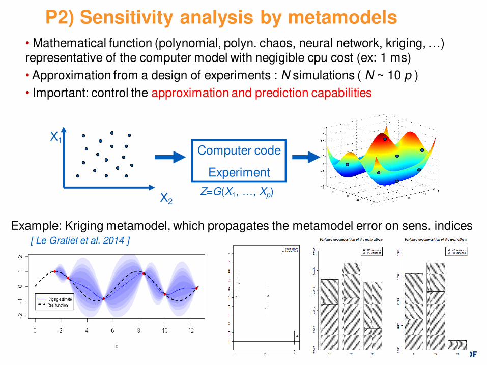
P2) Sensitivity analysis by metamodels

Computer code

Experiment

X1

X2

• Mathematical function (polynomial, polyn. chaos, neural network, kriging, …) representative of the computer model with negigible cpu cost (ex: 1 ms)

• Approximation from a design of experiments : N simulations ( N ~ 10 p )

• Important: control the approximation and prediction capabilities

Z=G(X1, …, Xp)

Example: Kriging metamodel, which propagates the metamodel error on sens. indices [ Le Gratiet et al. 2014 ]

Come-back to the flood model example – Output Cp

From the 100-size Monte Carlo sample, a Gaussian process metamodel is fitted

Predictivity of the Gp metamodel : Q2 = 99%

The previously shown formula are applied on the metamodel predictor

N=1e5

100 replicates

N x (p+2) x 100 = 7 x 107 metamodel evaluations

P3) Large p - Quantitative screening with HSICGeneralized sensitivity indices (HSIC) which not limit

SA to a single metric to compare change in the

distribution of the output when there an input varies

A dependence measure is used to compare the joint

distribution between Z and Xi and the product of marginals of Z and Xi with an infinityof metrics (kernel trick) => HSIC(Xi , Z), which is computed with a single sample

high-dimensional SA

Rem: classical indices (SRC, Sobol) only use the « mean » metric

[ Da Veiga 2015 ]

P3) Large p - Quantitative screening with DGSM (Derivative-based Global Sensitivity Measures)

Mix stochastic and deterministic approaches as global and local approaches

Inequality between DGSM and Sobol’ indices:

Cost (empirical) of evaluating the integral: N ~ 100 (smaller than for Sobol’ indices)

Cost of evaluating the derivatives:

p + 1 by finite differences

Independent of p if the adjoint models of f is available

high-dimensional SA

[ Kucherenko et al. 2009 ]

i

X

TiZ

fCS i

)Var(

)(0 :

iXfC constant [ Lamboni et al. 2013

Roustant et al. 2017 ]

)(

)Supp(

2

X

XX

Xd

X

G

i

i m

The idea is to pertub the pdf (prob. measure mi) of Xi by a statistics (e.g. the mean, variance, …). With a d perturbation, it gives the perturbed measure mid

Sensitivity indices on the QoI (e.g. a probability of failure P):

Two main technical ingredients:

- Minimisation of the Kullback-Leibler divergence

- Reverse importance sampling to estimate P and Pid using the same model outputs

Example :

P = Proba(model output > threshold)

Monte Carlo : N = 105, P = 9*10-4

Perturbation on the mean of each

input pdf

P5) Robustness analysis : PLI (Perturbed-Law based indices)

PP

i

PPP

P

P

P

ddd

dd ii

1111S ii

[ Lemaître et al. 2015 ]

XXXd

X

XP

ii

ii)G(i m

mm d

d)(

)(1 0

GumbelNormalTriangular

P5) Examples of perturbed probability laws

Mean perturbation:𝔼 𝑋𝑖 = 𝜇 + 𝛿

Variance perturbation𝔼 𝑋𝑖 = 𝜇Var 𝑋𝑖 = 𝜎2 + 𝛿

Normal Uniform

P5) Quantile-PLI – Analytical example

𝐺 𝑿 = 𝒔𝒊𝒏 𝑿𝟏 + 𝟕 ∗ 𝒔𝒊𝒏𝟐 𝑿𝟐 +𝟎, 𝟏 ∗ 𝑿𝟑𝟒 ∗ 𝒔𝒊𝒏 𝑿𝟏 ; 𝑿𝒊~𝑼 −𝝅,𝝅 independent

Sobol’ indices PLI on 𝑞95

The provided information are different

=> Robustness analysis for BEPU methodolology

[ Sueur et al. 2017 ]

Functional (in time) sensitivity indices

P6) Ubiquitous and aggregated indices

-0.8

-0.6

-0.4

-0.2

0

0.2

0.4

0.6

0 10 20 30 40 50 60 70 80 90 100

time (s)

se

ns

itiv

ity

P11

P12

P13

P14

P15

P16

P17

P18

P19

P20

Synthesize the information on sensitivity indices:

100 temporal output curves of the model

Aggregated sensitivity indices:

q

k

kik

i tSI

IGSI

1

[ Lamboni et al. 2009; Gamboa et al. 2014 ]

Output variance at time tk

Total output variance

P11P12P13P14P15P16

Conclusion: choosing the right method?

Requested information (qualitative/quantitative)

Number of inputs

Regularity of the model (linearity/monotony/continuity)

Cpu cost of one model evaluation

Number of outputs

Additional constraints, for example :

Uncertainty/sensitivity joint analysis,

Dependency between inputs, …

Recall: Main objectives of sensitivity analysis1. Understand the behaviour of the model (decompose input-output relations)

2. Simplify the computer model (dimension reduction)

Determine the non-influent variables (that can be fixed)

Determine the non-influent phenomena (to skip in the analysis)

Build a simplified model, a metamodel

3. Prioritize the uncertainty sources to reduce the model output uncertainty

- Variables to be fixed to obtain the largest output uncert. reduction

- Most influent variables in a given output domain

4. Analyze the robustness of the quantity of interest (QoI) with respect to the input uncertainty laws

Quantitative partitioning

Screening

Robustnessanalysis

(QoI= variability of the output)

Three types of answers:

1. Screening (qualitative information: influent/non influent)

- classical design of experiments,

- numerical design of experiments (Morris, sequential bifurcation)

2. Quantitative measures of global influence

- correlation/regression on values/ranks,

- functional variance decomposition (Sobol)

3. Deep exploration of sensitivities

- smoothing techniques (param./non parametric)

- metamodels

Recall: Methodology of SA

X1

X3

X2

Z

p 10p 1000p

Linear 1st

degre

Monotonic

2p

Morris

0

Non monotonic

N

Number of model

evaluations

Variance decomposition

Rank regression

Linear regression

Complexity/Regularityof the model G

Screening

Super screening

Sobol’ indices(direct

estimation)

Metamodel

Design ofexperiments

p-independent(N ~ 100)

Moment-independentSmoothing

Classification of methods[ Iooss & Saltelli 2017 ]

Fang et al., Design and modeling for computer experiments, Chapman & Hall, 2006

F. Gamboa, A. Janon, T. Klein, A. Lagnoux-Renaudie. Sensitivity analysis for multidimensional and functionaloutputs. Electronic Journal of Statistics. Volume 8, Number 1 (2014), 575-603.

J.C. Helton, J.D. Johnson, C.J. Salaberry et C.B. Storlie, Survey of sampling-based methods for uncertainty and sensitivity analysis. Reliability Engineering & System Safety, 91:1175 –1209, 2006

B. Iooss and L. Le Gratiet. Uncertainty and sensitivity analysis of functional risk curves based on Gaussian processes. Reliability Engineering and System Safety, In press

B. Iooss and A. Saltelli. Introduction: Sensitivity analysis. In: Handbook of uncertainty quantification, R. Ghanem, D. Higdon and H. Owhadi (Eds), Springer, 2017

Iooss and Lemaître. A review on global sensitivity analysis methods - In Uncertainty management in Simulation-Optimization of Complex Systems: Algorithms and Applications, C. Meloni and G. Dellino (eds), Springer, 2015 http://fr.arxiv.org/abs/1404.2405

Kleijnen, The design and analysis of simulation experiments, Springer, 2008

P. Lemaître, E. Sergienko, A. Arnaud, N. Bousquet, F. Gamboa and B. Iooss. Density modification basedreliability sensitivity analysis. Journal of Statistical Computation and Simulation, 85:1200-1223, 2015

A. Saltelli, K. Chan & E.M. Scott, Sensitivity analysis, Wiley, 2000

A. Saltelli et al., Global sensitivity analysis - The primer. Wiley, 2008

Bibliography